Cross-border bank flows, funding liquidity and house prices Chiara Banti and Kate Phylaktis *† Abstract The paper investigates the impact of global liquidity, proxied by funding liquidity, on house prices around the world. Focusing on the repo markets in US, Europe, UK and Japan, we document that changes in liquidity are related to cross-border bank flows and affect house prices. Highlighting the importance of looking beyond the US, we find that the liquidity effect depends on where liquidity has originated. Moreover, there is evidence of important banking and financial channels for liquidity shocks to house prices, especially in emerging markets. The exposure of house prices to liquidity shocks may be contained by certain country characteristics and policies. Keywords: global liquidity, house prices, repos. JEL classification: G15. 1 Introduction In the last decade, house prices around the world have registered a sustained upward trend, increas- ing on aggregate by around 30% from 1999 until the recent financial crisis. This pattern has been rather similar to that of cross-border bank flows that increased steadily (Figure 1, panel a). During this period, the correlation between changes in house prices and bank flows has been on average 36% for developed countries and 25% for emerging economies, and over 40% in some countries, such as Brazil, Canada, and Hong Kong. The increasing trend inverted during the recent financial crisis, * Chiara Banti, [email protected], Essex Business School, University of Essex, Wivenhoe Park, Colchester CO4 3SQ, UK; Corresponding author Professor Kate Phylaktis, [email protected], Faculty of Finance, Cass Business School, City University, 106 Bunhill Row, London, EC1Y 8TZ, UK, +44 (0)20 7040 8735. † We thank Rodrigo Alfaro, Carola Moreno, Claudio Raddatz, Barbara Ulloa and the participants at seminars at the Central Bank of Chile for useful comments. 1
Transcript
Cross-border bank flows, funding liquidity and house
prices
Chiara Banti and Kate Phylaktis∗†
Abstract
The paper investigates the impact of global liquidity, proxied by funding liquidity, on house
prices around the world. Focusing on the repo markets in US, Europe, UK and Japan, we
document that changes in liquidity are related to cross-border bank flows and affect house
prices. Highlighting the importance of looking beyond the US, we find that the liquidity effect
depends on where liquidity has originated. Moreover, there is evidence of important banking
and financial channels for liquidity shocks to house prices, especially in emerging markets. The
exposure of house prices to liquidity shocks may be contained by certain country characteristics
and policies.
Keywords: global liquidity, house prices, repos.
JEL classification: G15.
1 Introduction
In the last decade, house prices around the world have registered a sustained upward trend, increas-
ing on aggregate by around 30% from 1999 until the recent financial crisis. This pattern has been
rather similar to that of cross-border bank flows that increased steadily (Figure 1, panel a). During
this period, the correlation between changes in house prices and bank flows has been on average
36% for developed countries and 25% for emerging economies, and over 40% in some countries, such
as Brazil, Canada, and Hong Kong. The increasing trend inverted during the recent financial crisis,
∗Chiara Banti, [email protected], Essex Business School, University of Essex, Wivenhoe Park, Colchester CO4
3SQ, UK; Corresponding author Professor Kate Phylaktis, [email protected], Faculty of Finance, Cass Business
School, City University, 106 Bunhill Row, London, EC1Y 8TZ, UK, +44 (0)20 7040 8735.†We thank Rodrigo Alfaro, Carola Moreno, Claudio Raddatz, Barbara Ulloa and the participants at seminars at
the Central Bank of Chile for useful comments.
1
when key financial markets experienced severe liquidity dry-ups and credit conditions worsened
across the world. The responses of monetary authorities to the subsequent economic downturn
have unleashed unprecedented amounts of liquidity. During this period, both house prices and
bank flows resumed their upward trend. This is highlighted in Figure 1 (panel b), which presents
the annual growth rates of both cross bank flows and house prices for both developed and emerging
markets. While it is noticeable for both groups, the drop and subsequent recovery is more pro-
nounced in developed markets. This paper aims at investigating these dynamics and identifying
the relationship between house prices and global liquidity, that is the liquidity that crosses the
border and affects directly, or indirectly financing conditions abroad. In order to capture the global
liquidity dynamics relevant for house prices around the world, we focus on the private component of
liquidity on the major wholesale funding markets for financial intermediaries, that is the repurchase
agreement (repo) market not only in the US, but also in the UK, Europe and Japan. Changes in
the availability of financing in the main financial systems may affect house prices via the funding
channel that transmits global conditions into the local banking sector through bank flows. More-
over, funding conditions may also affect local house prices via their effect on the portfolio allocation
of major investors in real estate, such as hedge funds and real estate investment trusts (Baklanova,
Copeland, and Mccaughrin, 2015). Thus, after establishing the link between funding conditions
and bank flows, we study the impact of changes in funding availability in the main financial centers
on house prices around the world from 1999 to 2012 for a representative group of developed and
emerging markets.
We are making the following contributions to the literature. First, we introduce a different
proxy for global liquidity and use funding liquidity measured by funding aggregates, such as, the
repurchase agreements (repo).1 The impact of funding on the economy has also been investigated
by Chudik and Fratzscher (2011) and Cesa-Bianchi, Cespedes, and Rebucci (2015), but they use
financing costs and proxy it by the US TED spread. Chudik and Fratzscher (2011) concentrate
on the impact of financing costs during the global financial crisis, while Cesa-Bianchi et al. (2015)
use a longer time framework. However, as Figure 2 shows, funding costs have been extraordinarily
high during the recent financial crisis, making the variable more a proxy for the crisis episode
than a measure of funding liquidity over time. In this respect, we consider the pattern of funding
aggregates to capture more closely the evolution of funding availability through time. Moreover,
1Funding liquidity has been measured by repos in other works in different contexts e.g Banti and Phylaktis (2015);
Mancini Griffoli and Ranaldo (2011); Adrian, Etula, and Shin (2010); Coffey and Hrung (2009).
2
the amount outstanding of repos is a comprehensive measure of funding conditions that captures
also developments in market conditions, given the presence of collateral. Our proxy is related to
the bank leverage measure proposed by Bruno and Shin (2015), as it measures one of the sources of
financial institutions financing. However, it is specific to the availability of funding for investments
to the key players in the markets. In addition to an important source of wholesale funding for banks
(IMF, 2015), other important financial institutions, such as hedge funds and real estate investment
trusts, rely on repos to finance their operations (Baklanova et al., 2015). Nevertheless, we do
explore the impact of funding costs in our analysis, by introducing it as an interactive variable with
funding aggregates.
Secondly, we extend previous work by focusing on the international aspect of global liquidity
and consider changes in funding conditions not only in the US, but in other major financial systems,
Europe, UK, and Japan (Cerutti, Claessens, and Ratnovski, 2014). By taking this international
perspective, we establish not only the effects of global liquidity, but also where this liquidity has
originated. Thirdly, we do not treat the emerging markets as one homogeneous group. As Kuttner
(2015) notes in his discussion of the Cesa-Bianchi et al. (2015) study there are differences in the
relationship between global liquidity and house prices amongst emerging markets. The relationship
appears to be much tighter for the transition economies of Eastern and Central Europe compared
to Asia and Latin America during the 2000-2012 period. Thus, the results of Cesa-Bianchi et al.
(2015) on emerging markets might have been driven by what was going on in the Eastern and
Central European economies. Fourthly, we consider the characteristics of countries, which make
them less vulnerable to the transmission of global liquidity shocks. Finally we compare the relative
importance of global liquidity versus domestic monetary policy through variations in domestic
interest rates on house price developments. Although we have found global liquidity to impact
on house prices, the question arises whether it is sufficiently large to weaken the effectiveness of
domestic monetary policy in the presence of increased global liquidity.
To determine that the funding liquidity variable provides a good representation of global liq-
uidity, we first document that it is positively related to cross-border bank flows. Focusing on the
period from 1999 to 2012 due to data availability, we show that the impact of funding conditions on
different regions depends greatly on where it came from. While bank flows to developed countries
are affected by changes in funding conditions irrespective of their origin, emerging markets show a
more complex picture. Significantly related to US funding conditions, banks in emerging American
countries are also affected by liquidity conditions in Europe, while Asian banks by liquidity in
3
Japan. Also, banks in emerging Europe are exposed to global liquidity from Europe, and also from
Japan, when funding is tight. This is evidence of stronger regional linkages in emerging markets as
opposed to developed countries.
Having documented that funding conditions abroad affect flows into local banking sectors, we
proceed in our analysis and employ a panel vector autoregression (PVAR) to discern whether shifts
in funding conditions of the major financial centers impact house prices via the banking sector.
Using impulse response analysis we explore whether the local banking sector channels these shifts
on to the local housing market.
Our results can be summarized as follows. In line with previous findings, we document that
global liquidity triggers house price movements around the world (Darius and Radde, 2010; Till-
mann, 2013; Cesa-Bianchi et al., 2015). However, our analysis adds insights on this linkage. Indeed,
we find that the effect does not only originate from the US, but also from the other systematically
important financial systems. We find that house prices in developed countries react to liquidity
shocks irrespective of its origin. Emerging markets present again more regional linkages, with
emerging American prices affected by liquidity shocks in the US, emerging European house prices
affected by UK and EU liquidity and Asian house prices affected by liquidity shocks in Japan and
the UK. We find evidence that bank flows are a transmission mechanism for liquidity shocks to the
local housing markets, when shocks are transmitted to emerging markets. Conversely, the impact
on house prices of liquidity shocks in developed countries does not appear to be generally related to
banks. We find evidence however that major investors in real estate, such as real estate investment
trusts act also as a channel of liquidity shocks to the house market.
Moreover, this liquidity effect on house prices is associated to country characteristics and poli-
cies, such as bank regulation and supervision, and institution quality. Indeed, greater bank reg-
ulation, as well as exchange rate flexibility reduce the impact of liquidity shocks on local house
prices, but better institution quality increases it. Also, we find that restrictions to non-resident
investments in the local real estate sector are successful in mitigating the reactions of house prices
to liquidity shocks. These findings have policy implications for countries, which would like to limit
their exposure to global liquidity. Nevertheless, local governments can use monetary policy, in the
form of interest rate changes to offset the global liquidity impact on house prices in both developed
and emerging markets.
Our main results are robust to the use of a different bank flow data, the BIS data on cross-
border bank flows, instead of the IMF data. We have also checked the robustness of our VAR to a
4
structural break due to the crisis and found evidence that there is no structural break.
In the next section we review the related literature. In section 3, we describe the data and
provide some preliminary analysis. We present the empirical analysis of the relationship between
funding liquidity and cross-border bank flows in section 4. The empirical analysis of the impact
of changes in funding liquidity on house prices is reported in section 5. Section 6 investigates the
impact of domestic monetary policy on house prices and compares its impact to global liquidity,
while section 7 investigates the role of country characteristics and policies, which make a country
more vulnerable to global liquidity. Section 8 reports some robustness tests. Finally, section 9
concludes and reports some policy implications.
2 Literature Review
Our work draws from two strands of literature, the measurement of global liquidity and its trans-
mission, and the impact of global liquidity on asset prices, including house prices.2
Starting with Baks and Kramer (1999), global liquidity has been measured by money created
in the main financial centers. The rationale is that money created, in excess of the GDP growth,
will flow abroad to other financial systems and alter credit conditions in the recipient countries.
Empirical work on the relationship between monetary liquidity and asset prices provide mixed
evidence. While Darius and Radde (2010) and Belke, Orth, and Setzer (2010) document a positive
impact of liquidity on house prices, only a limited effect is found in Brana, Djigbenou, and Prat
(2012).
The recent interest in global liquidity led to the development of a more precise definition and
global liquidity has been associated with banks’ financing conditions across borders (Domanski,
Fender, and McGuire, 2011; Eickmeier, Gambacorta, and Hofmann, 2014). Given that monetary
aggregates fail to capture this cross-country bank flows, several works measure global liquidity by
employing credit aggregates. For instance, the BIS recently proposed its own indicators based on
cross-border bank debt flows (BIS, 2013).
Shin (2012) shows that permissive financing conditions are transmitted globally via cross-border
banking and global banks leverage. In their model of the international banking system, Bruno and
Shin (2015) contend that bank flows are affected by changes in the leverage of global banks. This
2The literature on house prices is vast. In this review we focus on the strand of the literature that studies house
price dynamics in the context of global liquidity, which is relevant for our work. See Agnello and Schuknecht (2009),
Duca, Muellbauer, and Murphy (2010) and Favilukis, Kohn, Ludvigson, and Van Nieuwerburgh (2011) for more
general recent reviews on the determinants of house prices.
5
implies that financing conditions in the main financial systems are transmitted across borders to the
local banking sector. In particular, changes in the size and leverage of systemically important banks
are the key push factors of bank flows. In the empirical application, Bruno and Shin (2015) measure
changes in financing conditions by the leverage of US dealers. Departing from a US-based approach,
Cerutti et al. (2014) show that global factors originating in the US, Europe, UK and Japan are
determinants of cross-border bank debt. These global factors include a measure of uncertainty
in the global financial markets, such as the VIX, and the US TED spread in addition to bank
leverage as measures of financing conditions. Also, they document a role for local country factors
on the extent to which global conditions affect cross-border bank flows. Finally, the importance of
funding considerations is documented in Cetorelli and Goldberg (2011). Employing a difference-
in-difference approach, they study the shock transmission mechanism from banks in developed to
banks in emerging countries. They find the main transmission mechanism to be the funding channel
to the banks in emerging countries as opposed to the cross-border direct lending or local lending
by foreign banks’ subsidiaries. Investigating the effect on Peruvian banks of Russia’s 1998 default,
Schnabl (2012) document that foreign lending amplifies external shocks while foreign ownership
mitigates them. In the light of this literature, we focus on funding aggregate measures in the main
financial centers to capture global liquidity conditions impact on cross-border bank flows.
Focusing on a panel of Asian countries, Tillmann (2013) find an overall positive effect of capital
flows on house prices, that is different across countries. Using a broader sample of countries and
focusing on funding costs, Chudik and Fratzscher (2011) and Cesa-Bianchi et al. (2015) investigate
the effect of global liquidity on the real economy of advanced and emerging economies. In more
detail, Chudik and Fratzscher (2011) study the shock transmission from the US to the real economy,
as measured by stock market prices, during the recent financial crisis in a global VAR. They find
that most emerging economies are affected by shifts in risk appetite, proxied by the VIX, while the
funding tightening has a key impact on advanced economies. Their measure of funding liquidity is
the US TED spread. In a panel VAR framework for a longer time period, Cesa-Bianchi et al. (2015)
document stronger impact of cross-border bank flows on house prices in a set of emerging markets
compared to advanced markets. To identify the effect of global liquidity, they employ a US-based
set of instruments related to global factors, including the TED spread and VIX. Similarly to the
above works, we investigate the reaction of house prices to liquidity in a panel VAR setting of 24
countries, which includes both developed and emerging economies, but extend the work in several
dimensions as explained earlier.
6
3 Data
In this section, we introduce the data used to measure our key variables, such as global liquidity,
bank flows and house prices.
3.1 Measuring global liquidity with repurchase agreements
Global liquidity is defined as the easing of financing conditions across borders and it has been
generally measured by credit aggregates, such as aggregated bank cross-border credit (BIS, 2013).
These proxies measure the outcome of liquidity, but cross-border credit is affected by factors other
than global liquidity, such as demand-side considerations (Domanski et al., 2011). Due to this,
some authors have employed alternative measures related to the supply of financing to identify
global liquidity, such as the VIX, the US TED spread and bank leverage measures (Chudik and
Fratzscher, 2011; Shin, 2012; Cerutti et al., 2014; Bruno and Shin, 2015; Cesa-Bianchi et al., 2015).
In line with the literature we focus on funding conditions to measure global liquidity. Differently to
previous work on liquidity and asset prices, we measure liquidity created not only in the US, but in
the UK, Europe and Japan as well, and we consider each system independently to determine where
global liquidity has originated (Cerutti et al., 2014). Moreover, we employ funding aggregates
in addition to costs to consider funding liquidity evolution. In fact, funding costs may be low
but funding may be generally rationed and only available to most creditworthy parties. Thus, we
consider funding aggregates to capture more accurately the evolution of funding availability through
time. To gather information on both aspects of funding conditions, we do include funding costs
in our analysis, as an interactive variable with funding aggregates.3 Finally, among the sources of
financing for financial institutions, we focus on repos that are a major source of wholesale financing
for financial institutions (IMF, 2015). Moreover, repos are collateralized debt instruments with
underlying assets. As such, their availability is affected by both funding and market conditions.
During the recent financial crisis, funding markets have experienced severe distress. While un-
secured interbank financing halted after Lehman Brothers bankruptcy and returned to be available
only to the most creditworthy counterparties after AIG bailout, severe uncertainty in the future
value of collateral led to a near collapse of the repo market in the US (Krishnamurthy, 2010; Afonso,
Kovner, and Schoar, 2011; Gorton and Metrick, 2012). As future expected volatility of the collat-
3An additional piece of information would be represented by the maturity of funding available (Banti and Phylaktis,
2015). In time of distress longer term financing is the most affected. However, we do not include this in our analysis
as data on maturity is only available for the US.
7
eral value increased, Gorton and Metrick (2012) show that haircuts raised and the range of assets
accepted as collateral was limited to the safest ones. In addition, after Lehman Brothers collapse,
transaction volume fell sharply, as agents engaged in large deleveraging and reduced their demand
for funding (Adrian and Shin, 2010; Krishnamurthy, 2010). Most recently, the IMF’s Global Fi-
nancial Stability Report has highlighted the vulnerabilities to the financial stability posed by the
current developments in the bond markets and their impact on collateralized lending (IMF, 2015).
By employing the amount outstanding of repos, we aim to consider both the funding and market
components of global liquidity. Given the presence of collateral our measure captures developments
in market conditions as well as financing.
Data on repos is available from the relevant Central Banks’ websites in domestic currency and
converted in USD with the IFS monthly exchange rates. In detail, US data on bilateral repos is
reported weekly by primary dealers to the Federal Reserve Bank of New York. Data on the repo
positions of monetary and financial institutions in the UK is reported monthly by the Bank of
England. Monthly repos of credit institutions in the Euro Area is available from the European
Central Bank. Finally, Japanese monthly payables under repos in the balance sheet of domestically
licensed banks is available from the Bank of Japan. Furthermore, we employ the Libor-OIS spread
as a proxy for the cost of funding, as it is highly correlated with the repo rate with Treasuries as
collateral in the US (Gorton and Metrick, 2012). The spread is the difference between 3-month
Libor rate and the Overnight Interest Swap for the US dollar, Euro, British pound and Japanese
yen. Data is collected from Datastream. The sample period starts in January 1999.
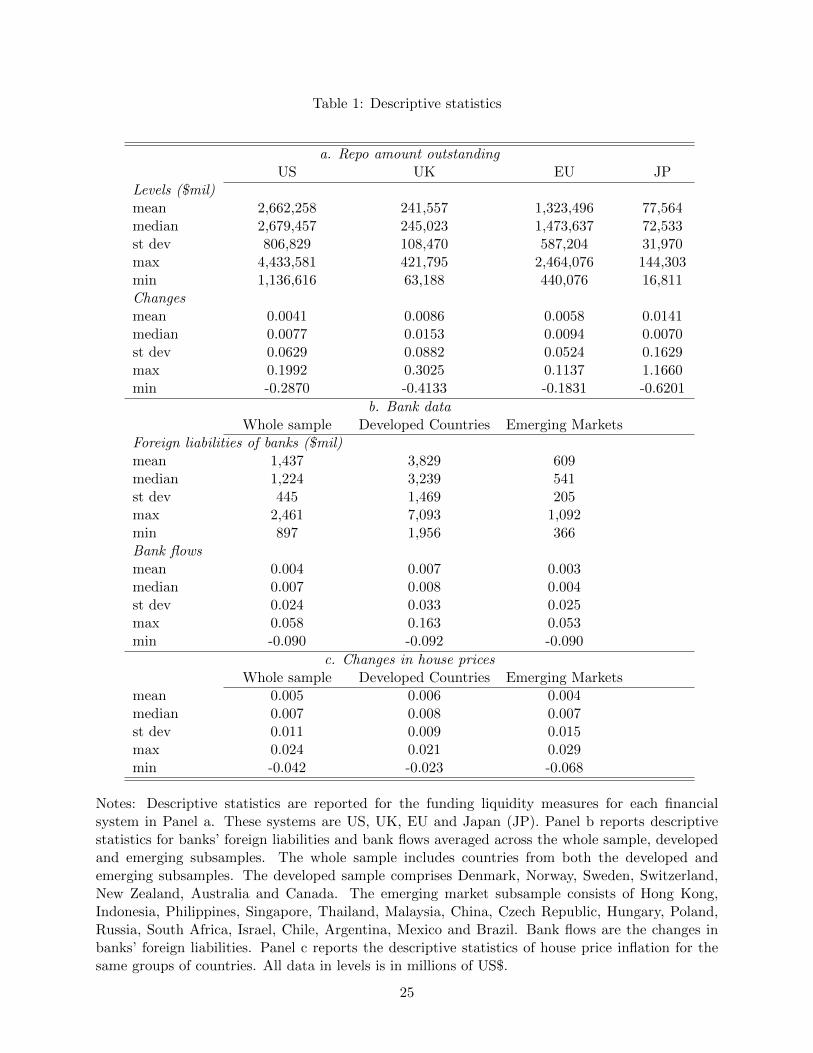
Table 1 (Panel a) reports the descriptive statistics of the repo data. The US repo market is the
largest, with an average amount outstanding of over $2tn, followed by the European repo market
with $1.3tn. The amount outstanding in the UK market is around $200bn, while the Japanese one
is $78bn.
3.2 Cross-border bank flows
To establish whether the funding liquidity measure captures global liquidity, we study the impact
of its changes on cross-border bank flows. To measure bank flows, we employ the changes in local
banks’ foreign liabilities from the International Financial Statistics (IFS). A frequently used dataset
in the literature is the BIS banking dataset that reports cross-border bank debt flows quarterly.4
4We have compared the series at quarterly frequency and found them to be highly correlated. As noted in Chung,
Lee, Loukoianova, Park, and Shin (2014), our data suffers from the limitation that some advanced countries do not
report in standardized formats.
8
The main reason for our choice is related to the monthly frequency of the IMF data, which allows
us to capture the dynamics more precisely and check whether our results are driven by the financial
crisis period.5 Nevertheless, we checked the robustness of our main results by using the BIS data
in section 8. All series are converted in USD and deflated with the US CPI.
The sample includes both developed and emerging countries and the choice is determined by the
availability of data for both bank flows and house prices. Following Chudik and Fratzscher (2011),
developed countries include Denmark, Norway, Sweden, Switzerland, New Zealand, Australia and
Canada. The emerging market subsample comprises countries from Asia, Europe and the Americas.
For Asia, the sample includes Hong Kong, Indonesia, Philippines, Singapore, Thailand, Malaysia
and China. Emerging Europe includes Czech Republic, Hungary, Poland, Russia, together with
South Africa and Israel. Finally, the Americas are Chile, Argentina, Mexico and Brazil.
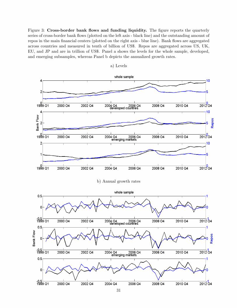
Graphical analysis in Figure 3 shows that cross-border bank flows share a common trend with
funding liquidity, especially in the drop following the recent financial crisis. Moreover, Table 1
(Panel b) reports the descriptive statistics of the data. The largest bank’s foreign liabilities are
in developed countries, with a monthly average of nearly $4tn, whereas emerging markets have
average monthly liabilities of around $600 millions. Similarly, bank flows expressed in percentage
of total liabilities are around 0.7% in developed countries. While nearly half than in developed
countries, bank flows of emerging markets exhibit more variability.
3.3 House price data
To measure house prices for the sample of countries described above we employ the dataset by
Cesa-Bianchi et al. (2015). House price data is available at quarterly frequency until 2012 and it is
collected from a variety of sources, such as local Statistics Offices, Central Banks and the BIS.
As the series exhibit non-stationarity, we take log-differences. Thus, the house price series
indicate real estate inflation in the relevant countries. Given the frequency of this data, the analysis
of the impact of shifts in funding conditions in the main financial systems on the local real estate
market is conducted at quarterly frequency.
Table 1 (Panel c) reports some descriptive statistics of house price changes. The average quar-
terly change in house prices for the period is around 0.5%. Similarly to bank flows, house prices in
emerging markets exhibit stronger variation than in developed ones.
5Our subsample analysis has revealed that our results are not driven by the crisis period. Results can be made
available on request by the authors.
9
4 Are funding liquidity conditions relevant for cross-border flows?
In the first step of our empirical analysis, we consider whether the banking sector is a channel for
funding liquidity shocks’ impact on house prices, and we look at the effect of liquidity conditions
in the main financial systems on cross-border bank flows.
Thus, we estimate a panel model of monthly changes in the foreign liabilities of banks in
each country on changes in funding liquidity conditions. We consider each main financial system
independently to determine where global liquidity has originated and run the following models:
∆Banki,t = β∆Fundst + δvixt + θ∆M st + γi + εt s = [US,UK,EU, JP ], (1)
where Banki,t are banks’ foreign liabilities in country i in month t in logs, Fundt is the outstanding
amount of repurchase agreements in the US, UK, EU and JP respectively in month t in logs, vixt
is a measure of financial market uncertainty (to account for the strong real effect of risk appetite
documented in Chudik and Fratzscher (2011)), Mt is broad money in the US, UK, EU and JP
respectively in month t in logs (to account for the role of money creation on liquidity), and γi are
country fixed effects. ∆ indicates changes. Standard errors are clustered at the country level.
Furthermore, we allow for an asymmetric impact of increases and decreases in funding liquidity:
∆Banki,t = β1(∆Fundst ∗ d
s,+t ) + β2(∆Fund
st ∗ d
s,−t ) + δvixt + θ∆M s
t + γi + εt
s = [US,UK,EU, JP ], (2)
where ds,+ is a dummy that takes the value of 1 when funding availability in the US, UK, EU and
JP respectively increases, and 0 otherwise and ds,− takes the value of 1 when funding decreases, and
0 otherwise. Moreover, to capture the full extent of funding liquidity moves, we consider funding
costs and interact our funding variable with a dummy for increases and decreases in the cost of
financing. To do so, we estimate the above model (2), where ds,+ is a dummy that takes the value
of 1 when funding costs in US, UK, EU and JP respectively increase, and 0 otherwise and ds,−
takes the value of 1 when funding costs decrease, and 0 otherwise.
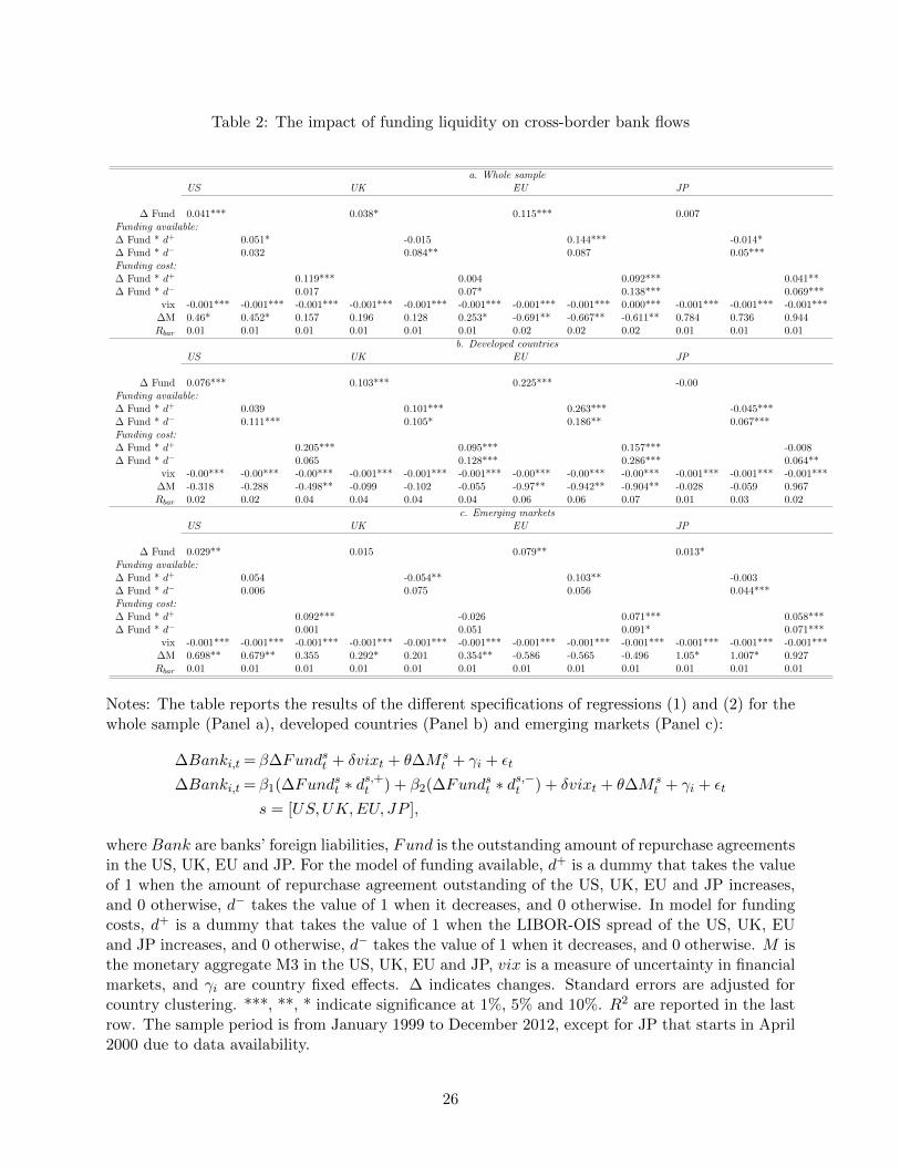
Table 2 reports the results for the whole sample of countries in Panel a. Bank flows are positively
related to changes in funding liquidity conditions in the US, EU and marginally in the UK. This
represents an increase in global liquidity, when liquidity conditions in the main financial systems
improve, enabling local banks to increase their foreign debt. While US and EU are significant
when liquidity increases, JP and UK funding are relevant when it is declining. Moreover, the
impact of US liquidity conditions is associated with periods of increasing funding costs. The VIX
10
is negative and significant in all models, as increasing uncertainty in the main financial centers is
associated with lower bank flows. For the monetary aggregates, the evidence is more mixed. It
is positively associated to bank flows in general, except for EU liquidity for which it exhibits a
negative relationship. These findings confirm the evidence provided in Cerutti et al. (2014) that
other financial systems in addition to the US are responsible for the creation of global liquidity
that affects bank flows.
Our sample contains a variety of countries at different stages of economic and financial develop-
ment. For this reason, we further investigate global liquidity by dividing our sample in developed
and emerging countries and estimating equations (1) and (2) for the two subsamples separately.
Table 2 reports the results for developed and emerging countries in Panels b and c respectively.
The findings confirm the role of US and EU funding liquidity conditions, whose changes strongly
affect bank flows in both developed and emerging countries. Changes in liquidity conditions in other
financial systems affect banks differently in different sub-samples. Indeed, bank flows in developed
countries are positively related to UK funding availability. Also, declines and increases in Japanese
liquidity are related to decreasing bank flows. This effect is stronger when funding costs decline.
In emerging countries, EU and US liquidity is significant in periods of increasing funding costs.
Japanese liquidity is a strong determinant of bank flows as declines in JP funding are associated
with less bank flows. Furthermore, bank flows decrease with increasing UK liquidity.
To offer further insights on the role of global liquidity on emerging markets, we look at individual
regions and conduct the analysis for countries in Asia, Europe and the Americas separately. The
evidence presented in Table 3 is rather diverse. In Panel a, Asian bank flows are strongly related
to Japanese funding liquidity, especially when declining and in periods of increasing funding costs.
Also, we find that liquidity in the US affects Asian banks in periods of increasing costs. In Panel
b, banks in emerging Europe are affected by EU and Japanese funding available when funding
costs increase. Finally, in Panel c, emerging American banks are affected by changes in liquidity
conditions in the US, EU and marginally the UK.
In conclusion, there is evidence of a strong impact of liquidity, proxied by funding aggregates and
generated in systemically important financial systems on the banking sector of both sub-samples of
countries. Banking flows in developed countries are generally related to liquidity generated across
the main financial systems, while in emerging markets they have more specific linkages.
11
5 Do funding liquidity conditions affect house prices?
In this section, we investigate whether shocks in funding conditions in the major financial centers
have an impact on house prices. Having documented that shifts in funding conditions abroad affect
flows into the local banking sectors, we now explore whether the local banking sector channels these
shifts on to the local housing market.
Thus, we estimate a panel vector autoregression (PVAR) model of funding liquidity and house
prices, including domestic variables such as real GDP growth and short term interest rates as
proxies for demand factors for housing, as follows:
Xsi,m =
N∑n=1
βiXsi,m−n + εi,m s = [US,UK,EU, JP ], (3)
where Xsi,m = [Fundsm, Gdpi,m, ri,m, P ricei,m], Price are house prices in country i, Gdp is real GDP
growth in country i, and r is the short term interest rate in country i. All variables except for Gdp
and r are in logs. We determine the number of lags n with the Schwarz criterion and it ranges
between 1 to 2 lags.
We focus separately on the impact of one standard deviation shock on funding liquidity in
each of the main financial centers on the local house prices across the main regional groups of our
sample of countries. To avoid imposing restrictions on the slope coefficients of house prices across
various countries, we employ the mean group estimator of Pesaran and Smith (1995). Thus, we
estimate a VAR for each country individually via OLS and estimate the impulse response functions
by employing the Cholesky decomposition of the covariance matrix of the VAR residuals. Since we
consider funding conditions in the main financial systems to be exogenous to domestic conditions
and local house prices, we order our funding variables first in all VARs. Moreover, we put house
prices last in the order to allow for both short-term interest rates and GDP growth to impact
house prices. We measure the average effect of the shock across countries by averaging cross-
country responses at each forecasting horizon, excluding the top and bottom 1%. The standard
errors of such measures are simply calculated as the cross-country variance of the responses at each
forecasting horizon, divided by the number of countries minus one (Pesaran and Smith, 1995).
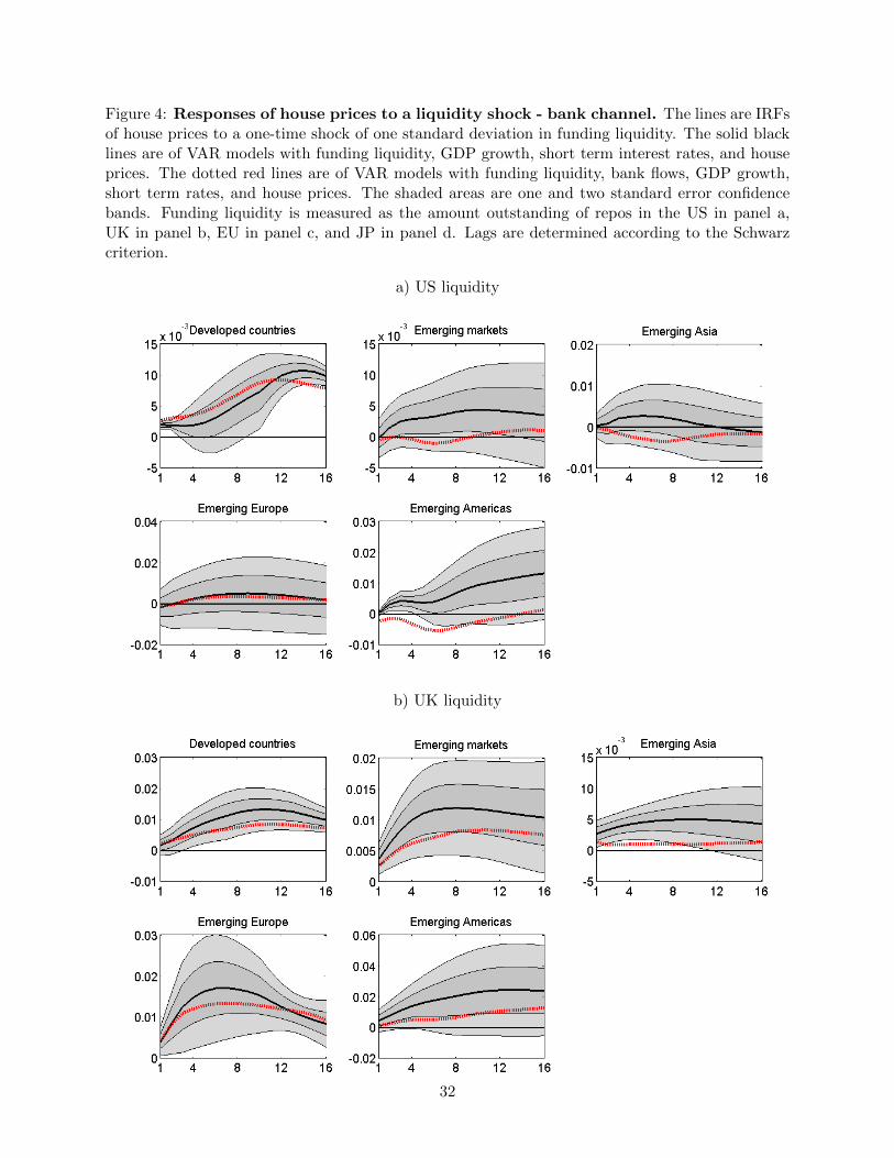
Figure 4 (panel a) reports the impulse response functions of house prices to shocks in US liq-
uidity. The reactions in house prices to liquidity shocks are stronger for the developed countries.
Moreover, among the emerging markets, Latin American housing prices exhibit the strongest reac-
tion to liquidity shocks. This finding is in line with the impact of US funding conditions on bank
flows.
12
UK and EU liquidity shocks affect both developed and emerging housing markets, with the
strongest reactions in emerging Europe (Figure 4, panels b and c). Moreover, house prices in Asia
are affected by liquidity shocks from the UK. Finally, Japanese liquidity shocks result in higher
house prices in Asia and in the developed countries subsample (Figure 4, panel d).
In conclusion, the analysis confirms a strong impact of liquidity on house prices in developed
countries irrespective of its origin. For emerging markets, the origin is instead very important.
Regional linkages are evident in our results, as European and Asian housing markets are affected
by liquidity originating in Europe (including the UK) and Japan, respectively. Nevertheless, we do
also find some more global impact. Indeed, Latin American house prices are affected by shocks in
the US and Asian house prices by shocks in the UK.
5.1 The role of transmission channels
In this section, we explore the role of banks and other institutional investors in the exposure of
local housing markets to unexpected shifts in global liquidity conditions.
Bank channel:
In order to identify the role of the banking sector on the transmission of shocks from funding
abroad on local house prices, we include bank flows into our model and estimate equation (3)
above with Xsi,m = [Fundsm, Banki,m, Gdpi,m, ri,m, P ricei,m]. We then compare the responses in
house prices of the model with and without bank flows. The dotted lines in Figure 4 represent
the reaction of house prices to the funding shock when bank flows are included in the VAR. If the
impact of funding on prices is channeled via bank flows, the reaction of house prices to funding
shocks should be reduced following the introduction of bank flows in the models (i.e. the dotted
line should be below the solid line if there is a significant bank channel).
We find that bank flows are a channel for US liquidity shocks on Latin American house prices.
Moreover, banks are channels for UK liquidity shocks for both developed and emerging countries,
especially in Asia. EU liquidity shocks are transmitted via banks to the emerging markets housing
prices. Finally, there is evidence of banks transmitting Japanese liquidity shocks to developed
countries’ housing markets.
In conclusion, we show that bank flows are relevant channels for the transmission of liquidity
shocks to house prices, especially in emerging markets. There is also some evidence of the role of
bank flows with respect to developed countries when the shocks originate in the UK and Japan.
13
Financial channel:
Banks are not the only potential channel. In fact, institutional investors that are important
international players, such as hedge funds and real estate investment trusts (reits) are affected
by shifts in funding liquidity in the main financial systems (Baklanova et al., 2015). If these
international investors participate in local real estate sectors by investing in stocks of firms operating
in the property sectors, then funding shocks abroad may be transmitted to local house prices via
the financial market. We measure the impact of these investors on house prices by employing the
GPR General Index that is the stock price index of all listed real estate companies with a market
capitalization in excess of 50 mil$ and over 75% of operations in the property sector. Data is
available from Global Property Research (GPR). The data coverage is not complete for our full
sample, and it excludes Hungary, Poland and Chile. Moreover, due to the limited number of time-
series observation, we drop Brazil, China, Czech Republic, Denmark, Israel, Mexico, and Russia.
Due to the limited cross-sectional dimension, we cannot estimate reliable responses and confidence
bands for the emerging market subsamples. For this reason, we limit the analysis in this section
to the developed and emerging groups. We build our quarterly series by taking the end-of-quarter
observation.
To identify this transmission channel, we include the real estate index (Indexi,m) in country
i into our model and estimate equation (3) above with Xsi,m = [Fundsm, Gdpi,m, ri,m, Indexi,m,
P ricei,m]. We then compare the responses in house prices of the model with and without the
index. The dotted lines in the Figure 5 are the reaction of house prices to the funding shock when
the index is included in the VAR. If the impact of funding on prices is channeled via the financial
market, the reaction of house prices to funding shocks should be reduced following the introduction
of the real estate index in the models (i.e. the dotted line should be below the solid line).
Overall, we find that the financial market is an important transmission channel for US liquidity
shocks to house prices in developed countries. Also, it is a channel for global liquidity shocks on
local house markets in emerging markets.
6 Impact of domestic monetary policy on house prices
Having found that global liquidity proxied by funding liquidity affects house prices, we go on to
investigate whether the monetary authorities can use monetary policy to offset its impact. In the
first instance, we investigate the impact of shocks to domestic monetary policy on local housing
markets, and consider the effect of a shock on domestic short-term interest rates on house prices.
14
Thus, using the VAR estimation of equation 3 we focus on the impact of one standard deviation
shock of the domestic short-term interest rates on the local house prices across the main regional
groups of our sample of countries.
As expected irrespective of the origin of global liquidity, there is a general negative reaction of
house prices in developed and emerging markets to shocks in domestic monetary policy. Turning
to the regions within the emerging countries, the effect is generally present in Asian and emerging
European house prices, but largely insignificant in Latin America. Results are not presented but
can be made available by the authors on request.
6.1 Forecast error variance decomposition
Having documented that domestic monetary policy through variations in domestic interest rates
has a negative impact, we perform forecast error variance decomposition to assess the relative role
of global liquidity versus domestic monetary policy on house price developments. In particular,
we compute the contribution of shocks to global liquidity and domestic short-term rates to the
forecast error variance of house prices for VAR models estimated for each country in the sample
as reported in Equation (3). We employ recursive re-formulation of the VAR model and use the
Cholesky decomposition to achieve orthogonal structural shocks.
Although we have found global liquidity to impact on house prices, the question arises whether
it is sufficiently large to weaken the effectiveness of domestic monetary policy in the presence of
increased global liquidity. An unanticipated increase in short term domestic interest rates consti-
tutes a contractionary monetary policy, which has been found as expected to have a dampening
effect on house prices. On the other hand an increase in global liquidity has a positive impact on
house prices.
In this exercise we present results in a more aggregated form. We present results for aggre-
gated liquidity, without distinguishing where liquidity has originated, on developed, and emerging
markets, as well as on the regional emerging market groups, i.e. Emerging Asia, Emerging Europe,
and Emerging Americas. We do not present results for each country separately, we average the
country results for each group. Table 4 shows the percentage of the total forecast error variance
of house prices at horizons of n={1,4,8,16} quarters that can be ascribed to global funding and to
domestic interest rate shocks. The variance decomposition reveals a different pattern for developed
and emerging markets. For the developed countries 11% of the forecast error variance 16 quarters
ahead can be ascribed to global liquidity shocks and 26% to domestic monetary policy shocks. That
15
implies that monetary policy is quite effective in developed markets in moderating the impact on
house prices arising from global liquidity. This finding is in line with the results of Darius and
Radde (2010), who using a monetary aggregate definition of global liquidity find that liquidity lost
completely predictive power of asset prices, including house prices in the G7 countries during the
2000s. Their explanation is that this is due to the expansionary monetary policies, which played a
much greater role than global factors in house price developments.
Looking now at emerging markets 22% of the forecast error variance 16 quarters ahead can be
ascribed to global liquidity shocks and 21% to domestic monetary policy shocks, that is monetary
policy is effective, but less so than in developed countries. This is more or less the same in all
emerging market regional groups. However, two further observations can be made. First, it seems
that emerging Americas are much more affected by liquidity shocks than developed countries and
any of the other emerging market regional groups. Secondly, the impact of global liquidity shocks
lingers on and in fact increases as time goes by in all groups.
7 The role of country characteristics
Having found that global liquidity affects house prices, we investigate whether some countries are
more vulnerable than others by looking at certain country characteristics and policies, which may
affect the exposure of house prices to external funding liquidity shocks. Thus, we follow the insights
in Cerutti et al. (2014), who investigated country characteristics, which may have affected bank
flows. We divide the full sample of countries according to the following characteristics and policies:
the regulatory environment of the local banking system, the general quality of the institutions,
the flexibility of the exchange rate, capital account openness and controls on real estate purchases
and sales by foreign investors. For each characteristic we estimate the VAR model in (3) with
funding liquidity and house prices as well as the other variables, as outlined in section 5. We
then aggregate the responses of house prices to liquidity shocks across countries that have more or
less of the characteristic than the cross-country median, individually. By examining the difference
in the IRFs from those above to those below the characteristic, we can determine whether the
characteristic is an important determinant of the exposure of the housing markets to global liquidity.
The results are presented in Figure 6. We take each characteristic in turn below:
The regulatory environment of the local banking sector : Focusing on the regulatory environment
of the local banking sector, we assess how its strength affects the exposure of house prices to
liquidity shocks. We measure the strength of bank regulation by the strength of capital adequacy
16
requirements and by the strength of supervisory power as developed by Barth, Caprio, and Levine
(2013) based on World Bank survey data. Relevant survey questions relate to information on
capital requirements (init cap strin) and power of the supervisory agencies (Sup Power). The
results show that house prices in countries with more stringent regulation are less strongly affected
by shocks in liquidity conditions.
The general quality of the institutions in the countries: We measure the institutions quality
with the index of economic freedom constructed by the Heritage Foundation.6 The index takes
into considerations several factors that affect the quality of countries’ institutions including prop-
erty rights, freedom from corruption, monetary freedom, trade freedom, investment freedom, and
financial freedom. The results show that countries with better institutions, attract more capital
and thus, are more exposed to liquidity shocks.
Flexibility of the exchange rate arrangements: We focus on the flexibility of the exchange rate
arrangements as a potential shield from external shocks on the local economies. Following Sham-
baugh (2004), exchange rate flexibility is calculated as the average across the full period of a
monthly dummy that takes the value of 1 if the exchange rate of the currency versus the reference
base (US$ or EUR) stays within a +/-2% band in a year, and 0 otherwise. We find that more
flexible exchange rates reduce the impact of global liquidity on house prices.
Capital account openness: We turn to the openness of the capital account of the countries, mea-
sured by the KAOPEN index (Ito and Chinn, 2006). The index is normalized to take values between
0 and 1 and it is the first principal component of proxies for regulatory controls of both current
and capital account transactions, for the existence of multiple exchange rates, and for requirements
on export proceeds. Higher values indicate greater openness. The results are inconclusive. This
could be due to the fact that the index is too general covering restrictions on both the current and
capital accounts. Thus we next investigated the impact of controls more specific to the housing
market and focused on the restrictions to the purchase and sale of real estate by non-residents.
Controls on real estate purchases and sales by foreign investors: This is measured by a dummy
that takes the value of 1 if restrictions are present and 0 otherwise, as developed by Fernandez,
Klein, Rebucci, Schindler, and Uribe (2015). The results show that house prices in countries with
more restrictions as expected are affected less by global liquidity.
In conclusion, we document that in addition to the banking and financial channels explored
in section 5, country characteristics and policies are important determinants of the exposure of
6The Heritage Foundation data is available at http://www.heritage.org/index/.
17
housing markets to global liquidity. In particular, we show that stronger bank regulation, and
more flexible exchange rates reduce the impact of liquidity shocks on local house prices. Moreover,
liquidity shocks affect more strongly countries with better institutional quality, more open capital
account and less restricted foreign investments in the real estate sector.
8 Robustness tests
8.1 The role of banking channel with alternative measure of bank flows
In the main analysis we measure bank flows as the foreign liabilities of local banks from the IMF.
We use this data because it is available at monthly frequency and it allows us to investigate whether
the impact of funding liquidity on bank flows are driven by the crisis period. Quarterly data would
not have been able to pick the beginning of the crisis.
In this section we conduct a robustness test of the analysis of the role of banking channel on
the transmission of liquidity shocks to house prices by employing the BIS data on cross-border
bank flows. Data is from the Locational BIS dataset and comprises the external claims (loans
and deposits) of reporting banks from all countries vis-a-vis the banking sector of the individual
countries in our sample. Data is in US$ and deflated with the US CPI.
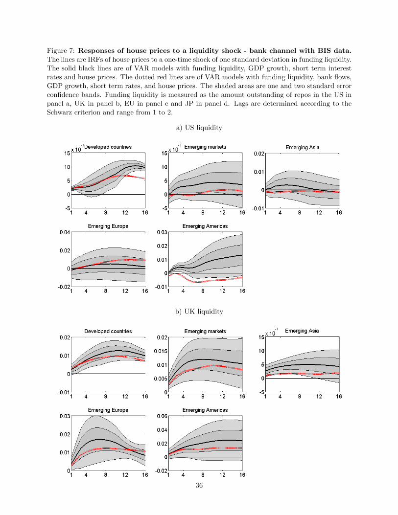
The results of the analysis of the banking channels are presented in Figure 7. We confirm the
main results in section 5. Indeed, we find that banks transmit the US liquidity shock on to Latin
American house prices. Also, there is evidence of transmission with respect to UK liquidity shocks
on both developed and emerging markets. Similarly to the main results, Japanese liquidity shocks
to developed countries’ housing markets are transmitted via banks channel too.
Differently than the main results, we find a stronger role of bank flows on developed countries
for liquidity shocks originating in all financial systems. In addition to the UK and Japan, we find
that liquidity shocks originating in the US and EU are transmitted via bank channels.
8.2 The recent financial crisis
As the crisis period may have affected several behavioral relationships, we investigate whether the
our VAR estimation is robust to the crisis episode, and check for breaks in the VAR during the
crisis. To do so, we conduct the Chow F-test for the significance of a dummy variable for the
crisis episode that takes the value of 1 for the period from 2007Q1 to 2008Q4, and 0 otherwise.
We estimate the VAR model in equation (3) for each country in our sample under two alternative
specifications: an unrestricted model including the dummy for the crisis period and a restricted
18
model where all coefficients of the dummy are set to zero. We test the null hypothesis that the
dummy variable coefficients are zero in all VAR equations, so that the restricted model is better
than the unrestricted model. We find that we cannot reject the null for the majority of countries
(over 60% of the sample) at the 5% significance level. Thus, we conclude that the crisis did not
cause a structural break in our VAR model.
9 Conclusion
The paper investigates the impact of global liquidity on house prices around the world. We in-
troduce a new measure of global liquidity, which focuses on the private component of liquidity on
the major wholesale funding markets for financial intermediaries, that is the repurchase agreement
(repo) market not only in the US, but also in the UK, Europe and Japan. Changes in the avail-
ability of financing in the main financial systems may affect house prices via the funding channel
that transmits global conditions into the local banking sector through bank flows. Thus, after
establishing the link between funding conditions and bank flows, we study the impact of changes
in funding availability in the main financial centers on house prices around the world from 1999 to
2012 for a representative group of developed and emerging markets.
In line with previous findings we document that global liquidity triggers house price movements
around the world (Darius and Radde, 2010; Tillmann, 2013; Cesa-Bianchi et al., 2015). However,
our analysis adds insights on this linkage. Indeed, we find that the effect does not only originate
from the US, but also from the other systematically important financial systems. We find that
house prices in developed countries react to liquidity shocks irrespective of its their origin. Emerging
markets present however more regional linkages, with emerging American prices affected by liquidity
shocks in the US, emerging European house prices affected by UK and EU liquidity, and Asian
house prices affected by liquidity shocks in Japan and the UK. Furthermore, we find evidence
that bank flows are a transmission mechanism for liquidity shocks to the local housing markets,
when shocks are transmitted to emerging markets. Conversely, the impact on house prices of
liquidity shocks in developed countries does not appear to be generally related to banks. Since
other important financial market players, such as hedge funds and real estate investment trusts,
rely on repos to finance their operations, we investigate whether real estate investment trusts act
also as a channel of liquidity to the house market. Our analysis shows that the investment trusts
are an important transmission channel for liquidity shocks originating in the US to house prices in
developed economies, while in emerging markets, it is a channel for all liquidity shocks, apart from
19
JP shocks.
Although we have found global liquidity to impact house prices, we have also established, that
governments in both developed and emerging markets can use monetary policy to offset part of that
impact. Furthermore, governments can implement more stringent bank regulation and supervision
measures, and more flexible exchange rates to reduce the impact of liquidity shocks on local house
prices. They can also adopt focused restrictions to non-resident investments in the local real estate
sector, which have been found to be effective in limiting the liquidity impact on house prices.
20
References
Adrian, T., Etula, E., Shin, H.S., 2010. Risk appetite and exchange rates. Federal Reserve Bank
of New York Staff Reports 361.
Adrian, T., Shin, H.S., 2010. Liquidity and leverage. Journal of Financial Intermediation 19,
418–437.
Afonso, G., Kovner, A., Schoar, A., 2011. Stressed, Not Frozen: The Federal Funds Market in the
Financial Crisis. Journal of Finance 66, 1109–1139.
Agnello, L., Schuknecht, L., 2009. Booms and Bust in Housing Market Determinants and Implica-
tions. ECB working paper .
Baklanova, V., Copeland, A., Mccaughrin, R., 2015. Reference Guide to U.S. Repo and Securities
Lending Markets. OFR working paper September.
Baks, K., Kramer, C., 1999. Global liquidity and asset prices: Measurement, implications, and
spillovers. IMF working paper 168.
Banti, C., Phylaktis, K., 2015. FX market liquidity, funding constraints and capital flows. Journal
of International Money and Finance 56, 114–134.
Barth, J.R., Caprio, G.J., Levine, R., 2013. Bank regulation and supervision in 180 countries from
1999 to 2011. Journal of Financial Economic Policy 5, 111–219.
Belke, A., Orth, W., Setzer, R., 2010. Liquidity and the dynamic pattern of asset price adjustment:
A global view. Journal of Banking & Finance 34, 1933–1945.
BIS, 2013. Triennial Central Bank Survey Foreign exchange turnover in April 2013: preliminary
global results. April.
Brana, S., Djigbenou, M.L., Prat, S., 2012. Global excess liquidity and asset prices in emerging
countries: A PVAR approach. Emerging Markets Review 135, 256–267.
Bruno, V., Shin, H.S., 2015. Cross-Border Banking and Global Liquidity. Review of Economic
Studies .
Cerutti, E., Claessens, S., Ratnovski, L., 2014. Global Liquidity and Drivers of Cross-Border Bank
Flows. IMF working paper 69.
21
Cesa-Bianchi, A., Cespedes, L.F., Rebucci, A., 2015. Capital Flows, House Prices, and the Macroe-
conomy: Evidence from Advanced and Emerging Market Economies. Journal of Money, Credit
and Banking 47, 301–335.
Cetorelli, N., Goldberg, L.S., 2011. Global Banks and International Shock Transmission: Evidence
from the Crisis. IMF Economic Review 59, 41–76.
Chudik, A., Fratzscher, M., 2011. Identifying the global transmission of the 2007-2009 financial
crisis in a GVAR model. European Economic Review 55, 325–339.
Chung, K., Lee, J.E., Loukoianova, E., Park, H., Shin, H.S., 2014. Global Liquidity through the
Lens of Monetary Aggregates. IMF Working Papers 14, 1.
Coffey, N., Hrung, W.B., 2009. Capital Constraints, Counterparty Risk, and Deviations from
Covered Interest Rate Parity. Federal Reserve Bank of New York Staff Reports 393.
Darius, R., Radde, S., 2010. Can Global Liquidity Forecast Asset Prices? IMF working paper 196.
Domanski, D., Fender, I., McGuire, P., 2011. Assessing global liquidity. BIS Quarterly Review
57–71.
Duca, J.V., Muellbauer, J., Murphy, A., 2010. Housing markets and the financial crisis of 20072009:
Lessons for the future. Journal of Financial Stability 6, 203–217.
Eickmeier, S., Gambacorta, L., Hofmann, B., 2014. Understanding global liquidity. European
Economic Review 68, 1–18.
Favilukis, J., Kohn, D., Ludvigson, S.C., Van Nieuwerburgh, S., 2011. International capital flows
and house prices: theory and evidence. NBER working paper series 17751.
Fernandez, A., Klein, M.W., Rebucci, A., Schindler, M., Uribe, M., 2015. Capital Control Measures:
A New Dataset. IMF working paper 80.
Gorton, G., Metrick, A., 2012. Securitized banking and the run on repo. Journal of Financial
Economics 104, 425–451.
IMF, 2015. Market liquidity - resilient or fleeting? Global Financial Stability Report October.
Ito, H., Chinn, M.D., 2006. What matters for financial development? Capital controls, institutions,
and interactions. Journal of Development Economics 81, 163–192.
22
Krishnamurthy, A., 2010. How Debt Markets Have Malfunctioned in the Crisis. Journal of Economic
Perspectives 24, 3–28.
Kuttner, K.N., 2015. Discussion of Cesa-Bianchi, Cespedes, and Rebucci. Journal of Money, Credit
and Banking 47, 337–342.
Mancini Griffoli, T.M., Ranaldo, A., 2011. Limits to arbitrage during the crisis: funding liquidity
constraints and covered interest parity. working paper .
Pesaran, M., Smith, R., 1995. Estimating long-run relationships from dynamic heterogeneous
panels, vol. 68.
Schnabl, P., 2012. The International Transmission of Bank Liquidity Shocks: Evidence from an
Emerging Market. Journal of Finance 67, 897–932.
Shambaugh, J.C., 2004. The Effect of Fixed Exchange Rates on Monetary Policy. Quarterly
Journal of Economics 119, 300–352.
Shin, H.S., 2012. Global Banking Glut and Loan Risk Premium. IMF Economic Review 60,
155–192.
Tillmann, P., 2013. Capital inflows and asset prices: Evidence from emerging Asia. Journal of
Banking and Finance 37, 717–729.
23
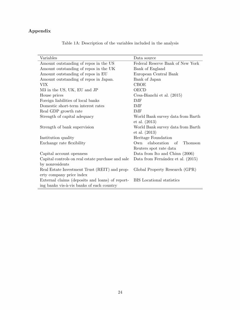
Appendix
Table 1A: Description of the variables included in the analysis
Variables Data source
Amount outstanding of repos in the US Federal Reserve Bank of New YorkAmount outstanding of repos in the UK Bank of EnglandAmount outstanding of repos in EU European Central BankAmount outstanding of repos in Japan. Bank of JapanVIX CBOEM3 in the US, UK, EU and JP OECDHouse prices Cesa-Bianchi et al. (2015)Foreign liabilities of local banks IMFDomestic short-term interest rates IMFReal GDP growth rate IMFStrength of capital adequacy World Bank survey data from Barth
et al. (2013)Strength of bank supervision World Bank survey data from Barth
et al. (2013)Institution quality Heritage FoundationExchange rate flexibility Own elaboration of Thomson
Reuters spot rate dataCapital account openness Data from Ito and Chinn (2006)Capital controls on real estate purchase and saleby nonresidents
Data from Fernandez et al. (2015)
Real Estate Investment Trust (REIT) and prop-erty company price index
Global Property Research (GPR)
External claims (deposits and loans) of report-ing banks vis-a-vis banks of each country
c. Changes in house pricesWhole sample Developed Countries Emerging Markets
mean 0.005 0.006 0.004median 0.007 0.008 0.007st dev 0.011 0.009 0.015max 0.024 0.021 0.029min -0.042 -0.023 -0.068
Notes: Descriptive statistics are reported for the funding liquidity measures for each financialsystem in Panel a. These systems are US, UK, EU and Japan (JP). Panel b reports descriptivestatistics for banks’ foreign liabilities and bank flows averaged across the whole sample, developedand emerging subsamples. The whole sample includes countries from both the developed andemerging subsamples. The developed sample comprises Denmark, Norway, Sweden, Switzerland,New Zealand, Australia and Canada. The emerging market subsample consists of Hong Kong,Indonesia, Philippines, Singapore, Thailand, Malaysia, China, Czech Republic, Hungary, Poland,Russia, South Africa, Israel, Chile, Argentina, Mexico and Brazil. Bank flows are the changes inbanks’ foreign liabilities. Panel c reports the descriptive statistics of house price inflation for thesame groups of countries. All data in levels is in millions of US$.
25
Table 2: The impact of funding liquidity on cross-border bank flows
a. Whole sampleUS UK EU JP
∆ Fund 0.041*** 0.038* 0.115*** 0.007Funding available:∆ Fund * d+ 0.051* -0.015 0.144*** -0.014*∆ Fund * d− 0.032 0.084** 0.087 0.05***Funding cost:∆ Fund * d+ 0.119*** 0.004 0.092*** 0.041**∆ Fund * d− 0.017 0.07* 0.138*** 0.069***
Notes: The table reports the results of the different specifications of regressions (1) and (2) for thewhole sample (Panel a), developed countries (Panel b) and emerging markets (Panel c):
∆Banki,t = β∆Fundst + δvixt + θ∆M st + γi + εt
∆Banki,t = β1(∆Fundst ∗ d
s,+t ) + β2(∆Fund
st ∗ d
s,−t ) + δvixt + θ∆M s
t + γi + εt
s = [US,UK,EU, JP ],
where Bank are banks’ foreign liabilities, Fund is the outstanding amount of repurchase agreementsin the US, UK, EU and JP. For the model of funding available, d+ is a dummy that takes the valueof 1 when the amount of repurchase agreement outstanding of the US, UK, EU and JP increases,and 0 otherwise, d− takes the value of 1 when it decreases, and 0 otherwise. In model for fundingcosts, d+ is a dummy that takes the value of 1 when the LIBOR-OIS spread of the US, UK, EUand JP increases, and 0 otherwise, d− takes the value of 1 when it decreases, and 0 otherwise. M isthe monetary aggregate M3 in the US, UK, EU and JP, vix is a measure of uncertainty in financialmarkets, and γi are country fixed effects. ∆ indicates changes. Standard errors are adjusted forcountry clustering. ***, **, * indicate significance at 1%, 5% and 10%. R2 are reported in the lastrow. The sample period is from January 1999 to December 2012, except for JP that starts in April2000 due to data availability.
26
Table 3: The impact of funding liquidity on cross-border bank flows in emerging markets
a. Emerging AsiaUS UK EU JP
∆ Fund 0.009 -0.004 0.018 0.031**Funding available:∆ Fund * d+ -0.021 -0.05 0.063* 0.002∆ Fund * d− 0.036 0.036 -0.026 0.089***Funding cost:∆ Fund * d+ 0.126*** -0.048 0.042 0.106***∆ Fund * d− -0.013 -0.012 0.001 0.078*
Notes: The table reports the results of the different specifications of regressions (1) and (2) for Asia(Panel a), emerging Europe (Panel b) and Latin America (Panel c):
∆Banki,t = β∆Fundst + δvixt + θ∆M st + γi + εt
∆Banki,t = β1(∆Fundst ∗ d
s,+t ) + β2(∆Fund
st ∗ d
s,−t ) + δvixt + θ∆M s
t + γi + εt
s = [US,UK,EU, JP ],
where Bank are banks’ foreign liabilities, Fund is the outstanding amount of repurchase agreementsin the US, UK, EU and JP. For the model of funding available, d+ is a dummy that takes the valueof 1 when the amount of repurchase agreement outstanding of the US, UK, EU and JP increases,and 0 otherwise, d− takes the value of 1 when it decreases, and 0 otherwise. In model for fundingcosts, d+ is a dummy that takes the value of 1 when the LIBOR-OIS spread of the US, UK, EUand JP increases, and 0 otherwise, d− takes the value of 1 when it decreases, and 0 otherwise. M isthe monetary aggregate M3 in the US, UK, EU and JP, vix is a measure of uncertainty in financialmarkets, and γi are country fixed effects. ∆ indicates changes. Standard errors are adjusted forcountry clustering. ***, **, * indicate significance at 1%, 5% and 10%. R2 are reported in the lastrow. The sample period is from January 1999 to December 2012, except for JP that starts in April2000 due to data availability.
27
Table 4: Forecast error variance decomposition
Developed countries Emerging marketsquarters Liquidity shock Rate shock Liquidity shock Rate shock
Notes: The table reports the forecast error variance decomposition of house prices of to shocksin funding liquidity and short-term interest rates. All VARs include funding liquidity, short-terminterest rates, real GDP growth and house prices. All variables except short-term rates and GDPare in logs. The sample period is from January 1999 to December 2012, except for JP that startsin April 2000 due to data availability.
28
Figure 1: House prices and cross-border bank flows. The figure reports the quarterly seriesof house prices (plotted on the left axis - black line) and cross-border bank flows (plotted on theright axis - blue line). House prices are the average across countries in the groups and are indexedto 100 in the second quarter of 2008. Bank flows are aggregated across countries and measured intenth of billion of US$. Panel a reports the levels for the whole sample, developed, and emergingsubsamples, whereas Panel b depicts the annualized growth rates.
a) Levels
b) Annual growth rates
29
Figure 2: Funding aggregate and cost. Monthly series of the amount outstanding of repurchaseagreements in the US (plotted on the left axis - solid line) and the US Libor-OIS spread (plottedon the right axis - dashed line). Repos are in million of US$, while the spread is in percentage.
30
Figure 3: Cross-border bank flows and funding liquidity. The figure reports the quarterlyseries of cross-border bank flows (plotted on the left axis - black line) and the outstanding amount ofrepos in the main financial centers (plotted on the right axis - blue line). Bank flows are aggregatedacross countries and measured in tenth of billion of US$. Repos are aggregated across US, UK,EU, and JP and are in trillion of US$. Panel a shows the levels for the whole sample, developed,and emerging subsamples, whereas Panel b depicts the annualized growth rates.
a) Levels
b) Annual growth rates
31
Figure 4: Responses of house prices to a liquidity shock - bank channel. The lines are IRFsof house prices to a one-time shock of one standard deviation in funding liquidity. The solid blacklines are of VAR models with funding liquidity, GDP growth, short term interest rates, and houseprices. The dotted red lines are of VAR models with funding liquidity, bank flows, GDP growth,short term rates, and house prices. The shaded areas are one and two standard error confidencebands. Funding liquidity is measured as the amount outstanding of repos in the US in panel a,UK in panel b, EU in panel c, and JP in panel d. Lags are determined according to the Schwarzcriterion.
a) US liquidity
b) UK liquidity
32
c) EU liquidity
d) JP liquidity
33
Figure 5: Responses of house prices to a liquidity shock - financial market channel. Thelines are IRFs of house prices to a one-time shock of one standard deviation in funding liquidity.The solid black lines are of VAR models with funding liquidity, GDP growth, short term interestrates, and house prices. The dotted red lines are of VAR models with funding liquidity, real estateindex, GDP growth, short term rates, and house prices. The shaded areas are one and two standarderror confidence bands. Funding liquidity is measured as the amount outstanding of repos in theUS in panel a, UK in panel b, EU in panel c, and JP in panel d. Lags are determined according tothe Schwarz criterion and range between 1 and 2.
a) US liquidity
b) UK liquidity
c) EU liquidity
d) JP liquidity
34
Figure 6: Responses of house prices to a funding shock for countries with higher (inblue) and lower (in red) country characteristics
The solid line represents the IRFs of house prices to a one time shock of one standard deviationin funding liquidity. The shaded areas are two standard error confidence bands. Country charac-teristics are described in the titles of the plots. They include the strength of capital regulation,bank supervision, institution quality, FX flexibility, capital openness, and controls on real estateinvestments by nonresidents. The blue responses are averaged across the sample of countries withhigher country characteristics than median. The red responses are averaged across the sample ofcountries with lower country characteristics than median. All VAR models have funding liquidity,real GDP growth, short-term interest rates, and house prices. Lags are determined according tothe Schwarz criterion.
35
Figure 7: Responses of house prices to a liquidity shock - bank channel with BIS data.The lines are IRFs of house prices to a one-time shock of one standard deviation in funding liquidity.The solid black lines are of VAR models with funding liquidity, GDP growth, short term interestrates and house prices. The dotted red lines are of VAR models with funding liquidity, bank flows,GDP growth, short term rates, and house prices. The shaded areas are one and two standard errorconfidence bands. Funding liquidity is measured as the amount outstanding of repos in the US inpanel a, UK in panel b, EU in panel c and JP in panel d. Lags are determined according to theSchwarz criterion and range from 1 to 2.