CS 361 – Chapter 1

• What is this class about?– Data structures, useful algorithm techniques– Programming needs to address both – You already have done some of this.– Analysis of algorithms to ensure an efficient solution.

Outline

• Ch.1 – Measuring complexity• Ch. 2-7 – Data structures• Ch. 8 – Sorting • Ch. 9-12 – Algorithm techniques• Ch. 13-16 – Applications to graphs, networks,

data compression, etc.• Special topics, e.g. order statistics, encryption,

convex hull, branch & bound, FFT

Data structures

• Data type vs. data structure

• What data structures have you used to hold your data?

• Why so many data structures?– Why not use an array for everything?

• Basic operations common to many/all data structures

Purpose of d.s.

• There is no data structure that’s perfect for all occasions. Each has specialized purpose or advantage.

• For a given problem, we want a d.s. that is especially efficient in certain ways.

• Ex. Consider insertions and deletions.– an equal number?– far more insertions than deletions?– Expected use of d.s. priority for which operations

should be most efficient.

Array list d.s.

• Java API has a built-in ArrayList class.– What can it do? – Why do we like it?– Anything wrong?

• What if we also had a “SortedArrayList” class that guaranteed that at all times the data is sorted….– Why might this be better than ArrayList?– But, is there a trade-off here?

Algorithm efficiency

• Suppose a problem has 2 solutions.– Implementation #1 requires n4 steps– Implementation #2 requires 2n steps

…where n is the size of the problem input.

• Assume 1 step can be done in 1 ns.

• Is one solution really “better” than the other? Why?

Execution time

Problem size (n) Time if n4 steps Time if 2n steps

2

5

10

20

100

Complete this table:

Execution time

Problem size (n) Time if n4 steps Time if 2n steps

2 16 ns 4 ns

5 625 ns 32 ns

10 10 μs 1 μs

20 160 μs 1 ms

100 0.1 s 1013 years

Approximate times assuming 1 step = 1 ns

Algorithm analysis

• 2 ways– Exact: “count” exact number of operations– Asymptotic: find asymptotic or upper bound

• Amortization– Technique to simplify calculation– E.g. consider effect of occasional time penalties

Exact analysis

• Not done often, only for small parts of code• We want # assembly instructions that execute.

– Easier to determine in C/C++/Java than Pascal/Ada because code is lower-level, more explicit.

• Control flow makes calculation interesting.• Example

for (i = 0; i < 10; ++i)

a[i] = i-1;– How many loop iterations?– How many instructions executed per iteration?– How many instructions are executed just once?– What if we replace 10 with n?

Example

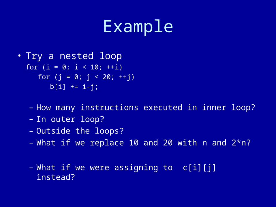
• Try a nested loopfor (i = 0; i < 10; ++i)

for (j = 0; j < 20; ++j)

b[i] += i-j;

– How many instructions executed in inner loop?– In outer loop?– Outside the loops?– What if we replace 10 and 20 with n and 2*n?

– What if we were assigning to c[i][j] instead?

Asymptotic analysis

• Much more often we are just interested in an order of magnitude, expressed as a function of some input size, n.– Essentially, it doesn’t matter much if the number of

steps is 5n2 or 7n2; any n2 is better than n3.

• Exact analysis is often unrealistic.– Usually too tedious.– There could be additional instructions behind the

scenes.– Not all instructions take the same amount of time.

Big O notation

• Provides an upper bound on the general complexity of an algorithm.– Ex. O(n2) means that it runs no worse than a quadratic

function of the input size.– O(n2) is a set of all functions at or below the complexity of

a degree 2 polynomial.

• Definition:

We say that f(n) is O(g(n)) if

constants c, n0 > 0 such that

f(n) c g(n) for all n > n0.

• “Eventually, g defeats f.”

Gist

• Usually, single loops are O(n), 2 nested loops are O(n2), etc.

• If the execution time of an algorithm is a polynomial in n, then we only need to keep the largest degree.

• We can drop coefficient.• Although O(…) is a set, we sometimes write “=“

for “is” or .• Let’s assume that our functions are positive.

Example loops

Loop Complexity

for (i = 1; i <= n; i = i + 1) O(n)

for (i = 1; i <= n; i = i * 2) O(log2(n))

for (i = 2; i <= n; i = i * i) O(log2(log2(n)))

for (i = 1; i * i <= n; i = i + 1) O(sqrt(n))

Example

• f(n) = 7n2 + 8n + 11 and g(n) = n2

• We want to show that f(n) is O(g(n))• How do we show this is true using the definition?

– We need to specify values of c and n0.

– We want to show that 7n2 + 8n + 11 <= c n2 for sufficiently large n.

– Note that 7n2 7n2, 8n 8n2, 11 11n2.

– So, let c = 7+8+11 = 26, and let n0 = 1.

– And we observe that for all n 0,

7n2 + 8n + 11 26 n2

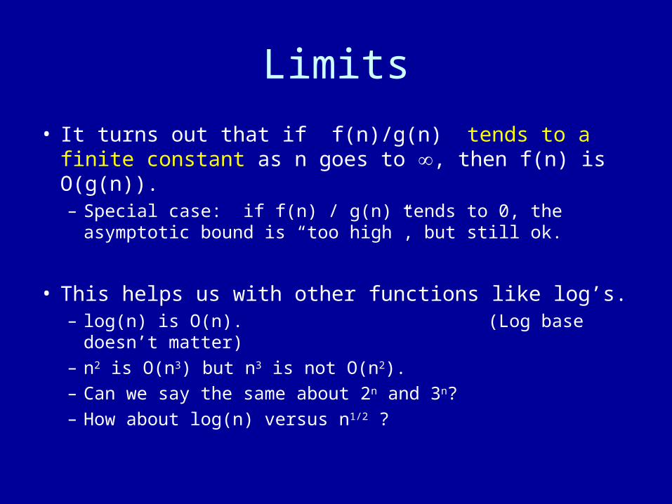
Limits

• It turns out that if f(n)/g(n) tends to a finite constant as n goes to , then f(n) is O(g(n)).– Special case: if f(n) / g(n) tends to 0, the asymptotic

bound is “too high”, but still ok.

• This helps us with other functions like log’s.– log(n) is O(n). (Log base doesn’t matter)– n2 is O(n3) but n3 is not O(n2).– Can we say the same about 2n and 3n?– How about log(n) versus n1/2 ?

Beyond O

• Big O has some close friends.– Big O: f(n) c g(n) for some c– Big Ω: f(n) c g(n) for some c– Big Θ: f is O(g) and g is O(f)

– Little o: f(n) c g(n) for all c– Little ω: f(n) c g(n) for all c

• What do the little letters mean?– f is o(g) means f has a strictly lower order than g.– Ex. n2 is o(n3) and o(n2 log n) but not o(n2).

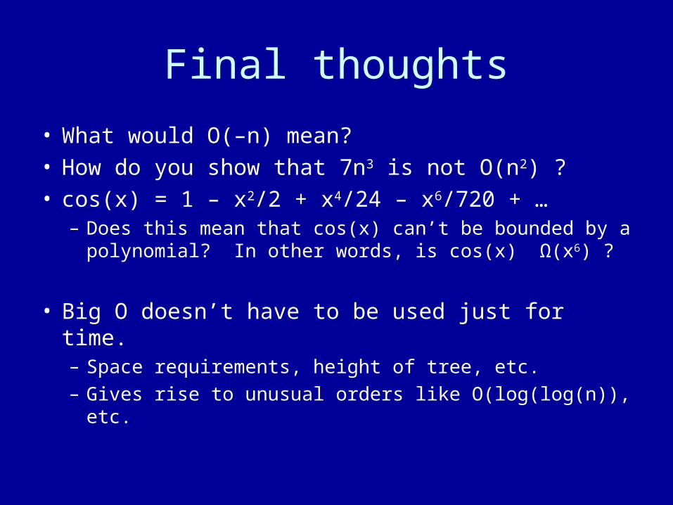
Final thoughts

• What would O(–n) mean?• How do you show that 7n3 is not O(n2) ?• cos(x) = 1 – x2/2 + x4/24 – x6/720 + …

– Does this mean that cos(x) can’t be bounded by a polynomial? In other words, is cos(x) Ω(x6) ?

• Big O doesn’t have to be used just for time.– Space requirements, height of tree, etc.– Gives rise to unusual orders like O(log(log(n)), etc.

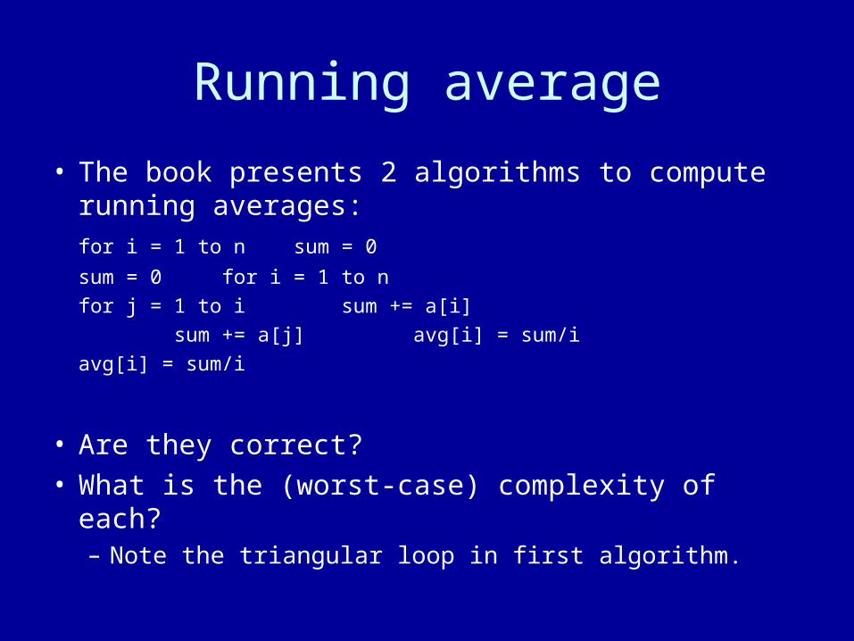
Running average

• The book presents 2 algorithms to compute running averages:for i = 1 to n sum = 0

sum = 0 for i = 1 to n

for j = 1 to i sum += a[i]

sum += a[j] avg[i] = sum/i

avg[i] = sum/i

• Are they correct?• What is the (worst-case) complexity of each?

– Note the triangular loop in first algorithm.

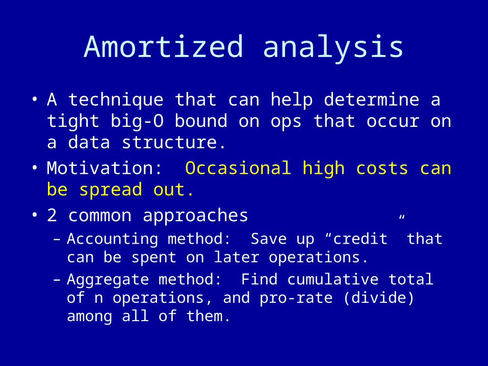
Amortized analysis

• A technique that can help determine a tight big-O bound on ops that occur on a data structure.

• Motivation: Occasional high costs can be spread out.

• 2 common approaches– Accounting method: Save up “credit” that can be

spent on later operations.– Aggregate method: Find cumulative total of n

operations, and pro-rate (divide) among all of them.

Accounting method

• We differentiate between actual & amortized cost of an operation.

• Some amortized costs will be “too high” so that others may become subsidized/free.

• At all times we want

amortized cost actual cost

so that we are in fact finding an upper bound.– In other words, early operations like “insert” assigned

a high cost so we keep a credit balance 0.

Accounting example

• Stack with 3 operations– Push: actual cost = 1– Pop: actual cost = 1– Multipop: actual cost = min(size, desired)

• What is the cost of performing n stack ops?– Naïve approach: There are n operations, and in the worst

case, a multipop operation must pop up to n elements, so n*n = O(n2).

– Better approach: Re-assess ops with amortized costs 2, 0, and 0, respectively. Rationale: Pushing an object will also “pay” for its later popping.

Thus: Total 2n = O(n). Average per op 2 = O(1).

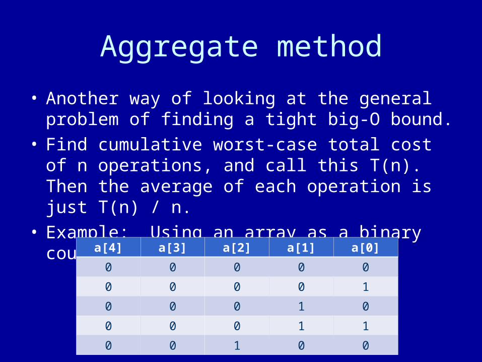
Aggregate method

• Another way of looking at the general problem of finding a tight big-O bound.

• Find cumulative worst-case total cost of n operations, and call this T(n). Then the average of each operation is just T(n) / n.

• Example: Using an array as a binary counter. a[4] a[3] a[2] a[1] a[0]

0 0 0 0 0

0 0 0 0 1

0 0 0 1 0

0 0 0 1 1

0 0 1 0 0

Binary counter

a = { 0 }

for i = 1 to n

// If rightmost bit is 0, set it to 1

if a[0] == 0

a[0] = 1

// Otherwise, working from right to left,

// turn off 1’s to 0’s until you reach a 0.

// Turn that 0 into a 1.

else

j = 0

while a[j] == 1

a[j++] = 0

a[j] = 1

Count the ops

a[4] A[3] A[2] A[1] A[0] # flips Run tot

0 0 0 0 0

0 0 0 0 1 1 1

0 0 0 1 0 2 3

0 0 0 1 1 1 4

0 0 1 0 0 3 7

0 0 1 0 1 1 8

0 0 1 1 0 2 10

0 0 1 1 1 1 11

0 1 0 0 0 4 15

0 1 0 0 1 1 16

0 1 0 1 0 2 18

0 1 0 1 1 1 19

Analysis

• Let the cost = # bit flips• Naïve: In counting from 0 to n, we may have to flip

several bits for each increment. And because we have a nested loop bounded by n, the algorithm is O(n2).

• Better way: Note that – a[0] is flipped on every iteration, – a[1] is flipped on every other iteration– a[2] is flipped on every 4th iteration, etc.– Total number of flips is 2n, so the total is O(n), and the

average number of flips per increment is O(1).

Exercise

• Suppose we have a data structure in which the cost of performing the i-th operation is– i, if i is a power of 2– 1, if i is not a power of 2

• Do either an accounting or aggregate analysis to find a tight big-O bound on: the total cost of n operations, and on the cost of a single operation.

• Work it out before checking your answer…

Solution

• Cost(i) = i, if i is a power of 2; 1 if not• We want an upper bound on the sum of cost(i) from i =

1 to n• Worst case is when n is a power of 2, e.g. 2k.• Then our sum is …

– All the powers of 2 from 1 thru 2k: 2 * 2k.

– 1 + 1 + 1 + … + 1, 2k times: 2k.

– Total is 3 * 2k, in other words 3n

• Thus, total cost of n operations is O(n), and average of each operation is O(1).– Surprising result?