CS194-24 Advanced Operating Systems Structures and Implementation Lecture 19 Disk Modeling File...

CS194-24Advanced Operating Systems

Structures and Implementation Lecture 19

Disk ModelingFile Systems Intro

April 15th, 2013Prof. John Kubiatowicz

http://inst.eecs.berkeley.edu/~cs194-24

Lec 19.24/15/13 Kubiatowicz CS194-24 ©UCB Fall 2013

Goals for Today

• Disk Drives and Queueing Theory• File Systems

Interactive is important!Ask Questions!

Note: Some slides and/or pictures in the following areadapted from slides ©2013


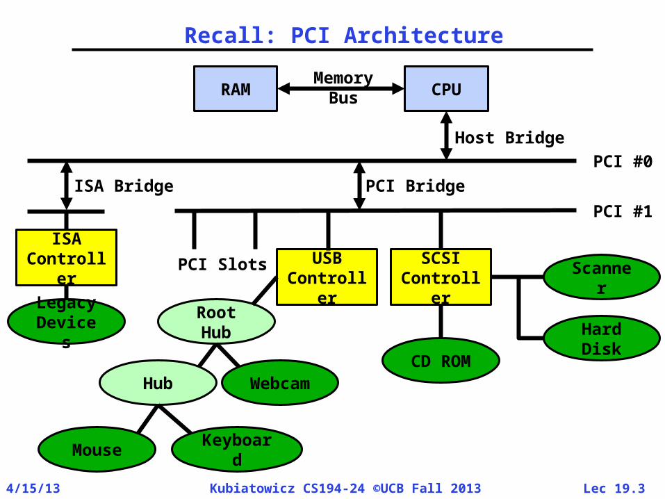
Recall: PCI Architecture

CPURAMMemory

Bus

USBControlle

r

SCSIControlle

r

Scanner

Hard DiskCD

ROM

Root Hub

HubWebca

m

MouseKeyboar

d

PCI #1

PCI #0

PCI Bridge

PCI Slots

Host Bridge

ISA Bridge

ISAControlle

rLegacyDevice

s


Recall: Device Drivers• Device Driver: Device-specific code in the kernel

that interacts directly with the device hardware– Supports a standard, internal interface– Same kernel I/O system can interact easily with

different device drivers– Special device-specific configuration supported with

the ioctl() system call• Linux Device drivers often installed via a Module

– Interface for dynamically loading code into kernel space

– Modules loaded with the “insmod” command and can contain parameters

• Driver-specific structure– One per driver– Contains a set of standard kernel interface routines

» Open: perform device-specific initialization» Read: perform read» Write: perform write» Release: perform device-specific shutdown» Etc.

– These routines registered at time device registered


Recall: I/O Device Notifying the OS• The OS needs to know when:

–The I/O device has completed an operation–The I/O operation has encountered an error

• I/O Interrupt:–Device generates an interrupt whenever it needs service

–Handled in top half of device driver» Often run on special kernel-level stack

–Pro: handles unpredictable events well–Con: interrupts relatively high overhead

• Polling:–OS periodically checks a device-specific status register» I/O device puts completion information in status

register» Could use timer to invoke upper half of drivers

occasionally–Pro: low overhead–Con: may waste many cycles on polling if infrequent or unpredictable I/O operations

• Actual devices combine both polling and interrupts–For instance: High-bandwidth network device:

» Interrupt for first incoming packet» Poll for following packets until hardware empty


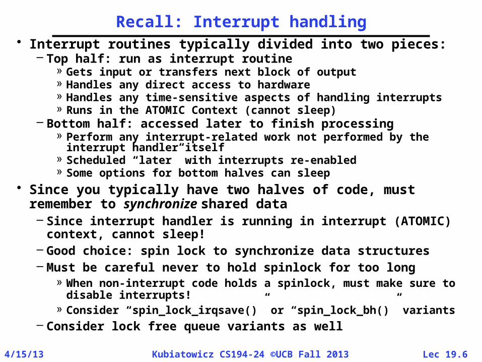
Recall: Interrupt handling• Interrupt routines typically divided into two pieces:

– Top half: run as interrupt routine» Gets input or transfers next block of output» Handles any direct access to hardware» Handles any time-sensitive aspects of handling interrupts» Runs in the ATOMIC Context (cannot sleep)

– Bottom half: accessed later to finish processing» Perform any interrupt-related work not performed by the

interrupt handler itself» Scheduled “later” with interrupts re-enabled» Some options for bottom halves can sleep

• Since you typically have two halves of code, must remember to synchronize shared data– Since interrupt handler is running in interrupt (ATOMIC)

context, cannot sleep!– Good choice: spin lock to synchronize data structures– Must be careful never to hold spinlock for too long

» When non-interrupt code holds a spinlock, must make sure to disable interrupts!

» Consider “spin_lock_irqsave()” or “spin_lock_bh()” variants

– Consider lock free queue variants as well


Hard Disk Drives

IBM/Hitachi Microdrive

Western Digital Drivehttp://www.storagereview.com/guide/

Read/Write HeadSide View


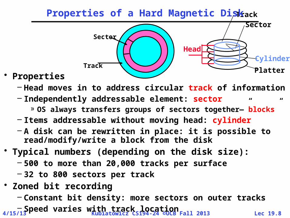
SectorTrack

Platter

Properties of a Hard Magnetic Disk

• Properties– Head moves in to address circular track of information– Independently addressable element: sector

» OS always transfers groups of sectors together—”blocks”– Items addressable without moving head: cylinder– A disk can be rewritten in place: it is possible to

read/modify/write a block from the disk• Typical numbers (depending on the disk size):

– 500 to more than 20,000 tracks per surface– 32 to 800 sectors per track

• Zoned bit recording– Constant bit density: more sectors on outer tracks– Speed varies with track location

Track

Sector

CylinderHead


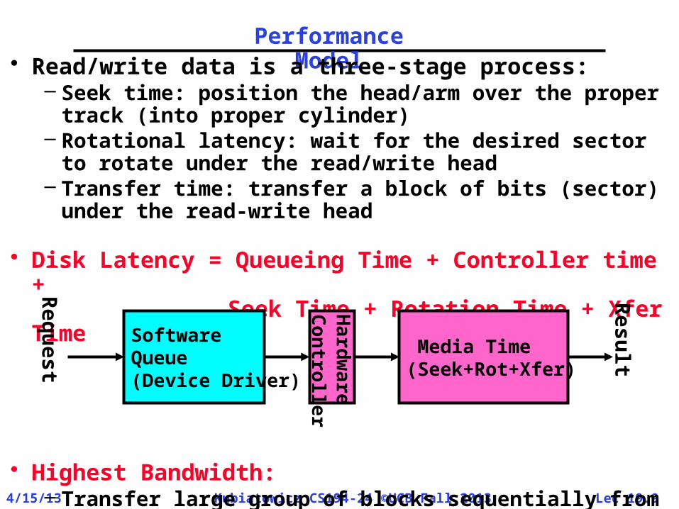
Performance Model• Read/write data is a three-stage process:

– Seek time: position the head/arm over the proper track (into proper cylinder)

– Rotational latency: wait for the desired sectorto rotate under the read/write head

– Transfer time: transfer a block of bits (sector)under the read-write head

• Disk Latency = Queueing Time + Controller time +

Seek Time + Rotation Time + Xfer Time

• Highest Bandwidth: – Transfer large group of blocks sequentially from

one track

SoftwareQueue(Device Driver)

Hard

ware

Con

trolle

r Media Time(Seek+Rot+Xfer)

Req

uest

Resu

lt


Typical Numbers of a Magnetic Disk• Specs for modern drives

– Space: 4TB in 3½ form factor (several manufacturers)

– Area Density: up around 570 GB/square inch for 4TB

• Average seek time as reported by the industry:– Typically in the range of 5 ms to 12 ms– Locality of reference may only be 25% to 33% of

the advertised number• Rotational Latency:

– Most disks rotate at 3,600 to 7200 RPM (Up to 15,000RPM or more)

– Approximately 16 ms to 8 ms per revolution, respectively

– An average latency to the desired information is halfway around the disk: 8 ms at 3600 RPM, 4 ms at 7200 RPM

• Transfer Time is a function of:– Transfer size (usually a sector): 512B – 1KB per

sector– Rotation speed: 3600 RPM to 15000 RPM– Recording density: bits per inch on a track– Diameter: ranges from 1 in to 5.25 in– Typical values: up to 180 MB per second

(systained)• Controller time depends on controller hardware


Example: Disk Performance

• Question: How long does it take to fetch 1 Kbyte sector?

• Assumptions:– Ignoring queuing and controller times for now– Avg seek time of 5ms, avg rotational delay of 4ms– Transfer rate of 4MByte/s, sector size of 1 KByte

• Random place on disk:– Seek (5ms) + Rot. Delay (4ms) + Transfer (0.25ms)– Roughly 10ms to fetch/put data: 100 KByte/sec

• Random place in same cylinder:– Rot. Delay (4ms) + Transfer (0.25ms)– Roughly 5ms to fetch/put data: 200 KByte/sec

• Next sector on same track:– Transfer (0.25ms): 4 MByte/sec

• Key to using disk effectively (esp. for filesystems) is to minimize seek and rotational delays


Properties of Magnetic Disk (Con’t)

• Performance of disk drive/file system– Metrics: Response Time, Throughput– Contributing factors to latency:

» Software paths (can be looselymodeled by a queue)

» Hardware controller» Physical disk media

• Queuing behavior:– Leads to big increases of latency

as utilization approaches 100% 100%

ResponseTime (ms)

Throughput (Utilization)(% total BW)

0

100

200

300

0%


A Little Queuing Theory: Some Results• Assumptions:

– System in equilibrium; No limit to the queue– Time between successive arrivals is random and

memoryless

• Parameters that describe our system:– : mean number of arriving customers/second– Tser: mean time to service a customer (“m1”)– C: squared coefficient of variance = 2/m12

– μ: service rate = 1/Tser– u: server utilization (0u1): u = /μ = Tser

• Parameters we wish to compute:– Tq: Time spent in queue– Lq: Length of queue = Tq (by Little’s law)

• Results:– Memoryless service distribution (C = 1):

» Called M/M/1 queue: Tq = Tser x u/(1 – u)– General service distribution (no restrictions), 1 server:

» Called M/G/1 queue: Tq = Tser x ½(1+C) x u/(1 – u))

Arrival Rate

Queue ServerService Rateμ=1/Tser


A Little Queuing Theory: An Example• Example Usage Statistics:

– User requests 10 8KB disk I/Os per second– Requests & service exponentially distributed

(C=1.0)– Avg. service = 20 ms

(controller+seek+rot+Xfertime)• Questions:

– How utilized is the disk? » Ans: server utilization, u = Tser– What is the average time spent in the queue? » Ans: Tq– What is the number of requests in the queue? » Ans: Lq = Tq– What is the avg response time for disk request? » Ans: Tsys = Tq + Tser (Wait in queue, then get served)

• Computation: (avg # arriving customers/s) = 10/sTser (avg time to service customer) = 20 ms (0.02s)u (server utilization) = Tser= 10/s .02s = 0.2Tq (avg time/customer in queue) = Tser u/(1 – u)

= 20 x 0.2/(1-0.2) = 20 0.25 = 5 ms (0 .005s)Lq (avg length of queue) = Tq=10/s .005s = 0.05Tsys (avg time/customer in system) =Tq + Tser= 25 ms


Administrivia

• Make sure to look through solutions for Midterm I– Try to get requests for regrades in by Next

Monday• Project 3 Code due on Thursday 4/25

– Get Going Now!!!– Device Driver Construction is Very Challenging

• Will be a short Project 4– Still working out the details

• Special Topics lecture– On Monday 5/8 during RRR week– What topics would you like me to talk about?

» Send me email!


Disk Scheduling• Disk can do only one request at a time; What

order do you choose to do queued requests?

• FIFO Order– Fair among requesters, but order of arrival may be

to random spots on the disk Very long seeks• SSTF: Shortest seek time first

– Pick the request that’s closest on the disk– Although called SSTF, today must include

rotational delay in calculation, since rotation can be as long as seek

– Con: SSTF good at reducing seeks, but may lead to starvation

• SCAN: Implements an Elevator Algorithm: take the closest request in the direction of travel– No starvation, but retains flavor of SSTF

• C-SCAN: Circular-Scan: only goes in one direction– Skips any requests on the way back– Fairer than SCAN, not biased towards pages in

middle

2,3

2,1

3,1

07,2

5,2

2,2 HeadUser

Requests

1

4

2

Dis

k H

ead

3


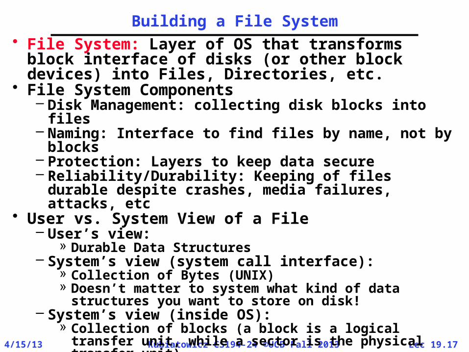
Building a File System• File System: Layer of OS that transforms block

interface of disks (or other block devices) into Files, Directories, etc.

• File System Components– Disk Management: collecting disk blocks into files– Naming: Interface to find files by name, not by

blocks– Protection: Layers to keep data secure– Reliability/Durability: Keeping of files durable

despite crashes, media failures, attacks, etc• User vs. System View of a File

– User’s view: » Durable Data Structures

– System’s view (system call interface):» Collection of Bytes (UNIX)» Doesn’t matter to system what kind of data

structures you want to store on disk!– System’s view (inside OS):

» Collection of blocks (a block is a logical transfer unit, while a sector is the physical transfer unit)

» Block size sector size; in UNIX, block size is 4KB


Translating from User to System View

• What happens if user says: give me bytes 2—12?– Fetch block corresponding to those bytes– Return just the correct portion of the block

• What about: write bytes 2—12?– Fetch block– Modify portion– Write out Block

• Everything inside File System is in whole size blocks– For example, getc(), putc() buffers something

like 4096 bytes, even if interface is one byte at a time

• From now on, file is a collection of blocks

FileSystem


Disk Management Policies• Basic entities on a disk:

– File: user-visible group of blocks arranged sequentially in logical space

– Directory: user-visible index mapping names to files (next lecture)

• Access disk as linear array of sectors. Two Options: – Identify sectors as vectors [cylinder, surface,

sector]. Sort in cylinder-major order. Not used much anymore.

– Logical Block Addressing (LBA). Every sector has integer address from zero up to max number of sectors.

– Controller translates from address physical position

» First case: OS/BIOS must deal with bad sectors» Second case: hardware shields OS from structure

of disk• Need way to track free disk blocks

– Link free blocks together too slow today– Use bitmap to represent free space on disk

• Need way to structure files: File Header– Track which blocks belong at which offsets within

the logical file structure– Optimize placement of files’ disk blocks to match

access and usage patterns


Designing the File System: Access Patterns

• How do users access files?– Need to know type of access patterns user is

likely to throw at system• Sequential Access: bytes read in order (“give

me the next X bytes, then give me next, etc”)– Almost all file access are of this flavor

• Random Access: read/write element out of middle of array (“give me bytes i—j”)– Less frequent, but still important. For example,

virtual memory backing file: page of memory stored in file

– Want this to be fast – don’t want to have to read all bytes to get to the middle of the file

• Content-based Access: (“find me 100 bytes starting with KUBIATOWICZ”)– Example: employee records – once you find the

bytes, increase my salary by a factor of 2– Many systems don’t provide this; instead,

databases are built on top of disk access to index content (requires efficient random access)


Designing the File System: Usage Patterns

• Most files are small (for example, .login, .c files)– A few files are big – nachos, core files, etc.; the

nachos executable is as big as all of your .class files combined

– However, most files are small – .class’s, .o’s, .c’s, etc.

• Large files use up most of the disk space and bandwidth to/from disk– May seem contradictory, but a few enormous files

are equivalent to an immense # of small files • Although we will use these observations,

beware usage patterns:– Good idea to look at usage patterns: beat

competitors by optimizing for frequent patterns– Except: changes in performance or cost can alter

usage patterns. Maybe UNIX has lots of small files because big files are really inefficient?


How to organize files on disk

• Goals:– Maximize sequential performance– Easy random access to file– Easy management of file (growth, truncation, etc)

• First Technique: Continuous Allocation– Use continuous range of blocks in logical block space

» Analogous to base+bounds in virtual memory» User says in advance how big file will be

(disadvantage)– Search bit-map for space using best fit/first fit

» What if not enough contiguous space for new file?– File Header Contains:

» First sector/LBA in file» File size (# of sectors)

– Pros: Fast Sequential Access, Easy Random access– Cons: External Fragmentation/Hard to grow files

» Free holes get smaller and smaller» Could compact space, but that would be really

expensive• Continuous Allocation used by IBM 360

– Result of allocation and management cost: People would create a big file, put their file in the middle


Linked List Allocation

• Second Technique: Linked List Approach– Each block, pointer to next on disk

– Pros: Can grow files dynamically, Free list same as file

– Cons: Bad Sequential Access (seek between each block), Unreliable (lose block, lose rest of file)

– Serious Con: Bad random access!!!!– Technique originally from Alto (First PC, built at

Xerox)» No attempt to allocate contiguous blocks

Null

File Header


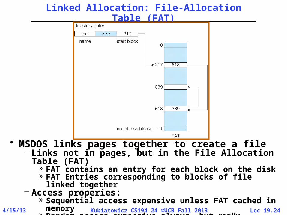
Linked Allocation: File-Allocation Table (FAT)

• MSDOS links pages together to create a file– Links not in pages, but in the File Allocation Table

(FAT)» FAT contains an entry for each block on the disk» FAT Entries corresponding to blocks of file linked

together– Access properies:

» Sequential access expensive unless FAT cached in memory

» Random access expensive always, but really expensive if FAT not cached in memory


Indexed Allocation

• Indexed Files (Nachos, VMS)– System Allocates file header block to hold array of

pointers big enough to point to all blocks» User pre-declares max file size;

– Pros: Can easily grow up to space allocated for index Random access is fast

– Cons: Clumsy to grow file bigger than table sizeStill lots of seeks: blocks may be spread

over disk


Multilevel Indexed Files (UNIX BSD 4.1) • Multilevel Indexed Files: Like multilevel

address translation (from UNIX 4.1 BSD)– Key idea: efficient for small files, but still allow

big files– File header contains 13 pointers

» Fixed size table, pointers not all equivalent» This header is called an “inode” in UNIX

– File Header format:» First 10 pointers are to data blocks» Block 11 points to “indirect block” containing 256

blocks» Block 12 points to “doubly indirect block”

containing 256 indirect blocks for total of 64K blocks

» Block 13 points to a triply indirect block (16M blocks)

• Discussion– Basic technique places an upper limit on file size

that is approximately 16Gbytes» Designers thought this was bigger than anything

anyone would need. Much bigger than a disk at the time…

» Fallacy: today, EOS producing 2TB of data per day– Pointers get filled in dynamically: need to

allocate indirect block only when file grows > 10 blocks.

» On small files, no indirection needed


Example of Multilevel Indexed Files• Sample file in multilevel

indexed format:– How many accesses for

block #23? (assume file header accessed on open)?

» Two: One for indirect block, one for data

– How about block #5?» One: One for data

– Block #340?» Three: double indirect block,

indirect block, and data• UNIX 4.1 Pros and cons

– Pros: Simple (more or less)Files can easily expand (up to a point)Small files particularly cheap and easy

– Cons: Lots of seeksVery large files must read many indirect

block (four I/Os per block!)


Conclusion• Multilevel Indexed Scheme

– Inode contains file info, direct pointers to blocks, – indirect blocks, doubly indirect, etc..

• Cray DEMOS: optimization for sequential access– Inode holds set of disk ranges, similar to

segmentation• 4.2 BSD Multilevel index files

– Inode contains pointers to actual blocks, indirect blocks, double indirect blocks, etc

– Optimizations for sequential access: start new files in open ranges of free blocks

– Rotational Optimization• Naming: act of translating from user-visible

names to actual system resources– Directories used for naming for local file systems

• Important system properties– Availability: how often is the resource available?– Durability: how well is data preserved against

faults?– Reliability: how often is resource performing

correctly?

Date post:	27-Dec-2015
Category:	Documents
Upload:	eleanore-french
View:	221 times
Download:	2 times

CS194-24 Advanced Operating Systems Structures and Implementation Lecture 19 Disk Modeling File...

Documents