53
CS215 Logic Programming with Prolog ' mario camilleri 1991/3

CS215 Logic Programming with Prolog
© mario camilleri 1991/3

i
Table of Contents
Table of Contents ....................................................................................................... i
1 Introduction.........................................................................................................1 1.1 Texts .............................................................................................................................. 1 1.2 Supplementary texts: ..................................................................................................... 1 1.3 Software ........................................................................................................................ 2 1.4 Assessment Procedure ................................................................................................... 2
2 Preliminary material � propositional logic........................................................3 2.1 The Syntax of Propositional Logic................................................................................ 3 2.2 The Semantics of Propositional Logic........................................................................... 3 2.3 Satisfiability................................................................................................................... 4 2.4 Conjunctive Normal Form............................................................................................. 4 2.5 Logical Consequence .................................................................................................... 5 2.6 Deduction Principle ....................................................................................................... 5 2.7 Deduction as a computational principle ........................................................................ 5
3 Resolution and Horn Clauses............................................................................7 3.1 Deduction Procedures.................................................................................................... 7 3.2 Semantic Trees .............................................................................................................. 8 3.3 Failure Nodes ................................................................................................................ 8 3.4 Failure Trees and Inference Nodes................................................................................ 8 3.5 Properties of Failure Trees ............................................................................................ 9 3.6 The Resolution Principle ............................................................................................... 9 3.7 Completeness of Resolution in Propositional Logic ................................................... 10 3.8 Inconsistency proofs based on Resolution .................................................................. 11 3.9 Non-Determinism in Resolution Refutations .............................................................. 11 3.10 Horn-Clause Logic ...................................................................................................... 11 3.11 Horn-Clause Logic Programs ...................................................................................... 12 3.12 Exercises...................................................................................................................... 12
4 The Language Proplog .....................................................................................14 4.1 Some Syntactic Sugar.................................................................................................. 14 4.2 Horn Clauses and Rewriting Rules.............................................................................. 14 4.3 PropLog....................................................................................................................... 15 4.4 SLD-Resolution........................................................................................................... 16 4.5 OR-Trees ..................................................................................................................... 17 4.6 Search Strategies ......................................................................................................... 17 4.7 The Closed-World Assumption and Negation by Failure ........................................... 18

ii
5 Datalog...............................................................................................................19 5.1 DataLog....................................................................................................................... 19 5.2 Relations......................................................................................................................19 5.3 Predicates..................................................................................................................... 19 5.4 Family relations ........................................................................................................... 20 5.5 Queries and Unification............................................................................................... 20 5.6 Queries and logic Variables......................................................................................... 20 5.7 Rules............................................................................................................................ 21 5.8 Commutativity ............................................................................................................. 21 5.9 Transitivity .................................................................................................................. 21 5.10 Mixing Facts and Rules ............................................................................................... 22 5.11 Recursive Rules ........................................................................................................... 22 5.12 Components of Datalog............................................................................................... 22 5.13 The Unification Mechanism ........................................................................................ 23 5.14 Scope of Named Variables .......................................................................................... 24 5.15 Scope of the Anonymous Variable.............................................................................. 24 5.16 Exercises...................................................................................................................... 24
6 Prolog ................................................................................................................26 6.1 Compound Terms as Data ........................................................................................... 26 6.2 Reversibility and Extra logical Predicates................................................................... 26 6.3 Term Classification Predicates .................................................................................... 27 6.4 Controlling Backtracking: the ! (Cut) Inbuilt Predicate .............................................. 27 6.5 The fail Inbuilt Predicate ............................................................................................. 28 6.6 Terms as Literals ......................................................................................................... 28 6.7 Arithmetic Expression Trees ....................................................................................... 28 6.8 Operator Syntax........................................................................................................... 29 6.9 The is and = Infix Operators........................................................................................ 29 6.10 Constant Folding ......................................................................................................... 29 6.11 Exercises...................................................................................................................... 30
7 Lists in Prolog...................................................................................................32 7.1 Representing Lists using Compound Terms................................................................ 32 7.2 Operations on Lists...................................................................................................... 32 7.3 Adding Syntactic Sugar............................................................................................... 32 7.4 Unification on Lists ..................................................................................................... 33 7.5 Elementary List Predicates .......................................................................................... 33 7.6 The nth Element of a List ............................................................................................ 33 7.7 Appending Lists .......................................................................................................... 34 7.8 Reversing a List........................................................................................................... 34 7.9 Deleting and Replacing Elements from a List ............................................................. 34 7.10 List Application........................................................................................................... 35 7.11 List Mapping ............................................................................................................... 35 7.12 Exercises...................................................................................................................... 36
8 The Unification Mechanism .............................................................................37 8.1 Instances of Universally Quantified Clauses............................................................... 37 8.2 Substitutions ................................................................................................................ 38 8.3 The Idempotence Constraint........................................................................................ 38 8.4 Composition of Substitutions ...................................................................................... 38 8.5 Unifiers........................................................................................................................ 39 8.6 Unification Algorithms................................................................................................ 39 8.7 Prolog and Cyclic Structures ....................................................................................... 40 8.8 Constraint Logic Programming ................................................................................... 40 8.9 CLP Languages ........................................................................................................... 41 8.10 Examples of CLP Programs ........................................................................................ 41
Generating 8086-assembly code for a Pascal assignment statement. ...............44
Rewriting propositional formulae into simplified, nand-2 form. .........................46

iii
Symbolic manipulation of algebraic expressions. ...............................................47
Tangles, Knots and Unknots ..................................................................................48

mario camilleri 1993
Introduction Page 1
1 Introduction
Logic programming takes proof theory as the model of computation. A logic program is a set of axioms, a logic interpreter implements a deduction mechanism based on some inference rule or rules, and the object of a computation is to determine which conclusions follow (or whether a particular statement of interest follows) from the axioms and the inference rules. Historically, logic programming is linked with the language Prolog, developed in the early 1970s from research in natural-language processing. Although still the only language of its kind, Prolog must be viewed as a TOOL � a practical, working implementations of the concepts behind logic programming. Because it introduces certain impurities, we must carefully distinguish between Prolog the language and logic programming the concept.
1.1 Texts Recommended texts: • Clocksin,W.F. and Mellish,C.S. (1987 3rd edn) Programming in Prolog, Springer-Verlag
ISBN 3-540-17539-3
• Sterling,L. and Shapiro,E. (1994 2nd edn) The Art of Prolog, MIT Press London ISBN 0-262-19338-8
1.2 Supplementary texts: • Gallier,J.H. (1987) Logic for Computer Science, John Wiley
ISBN 0-471-61546-3
• Chang, C.L. and Lee, R. C. (1973) Symbolic Logic and Mechanical Theorem Proving, Academic Press. ISBN 0-12-170350-9
• Thayse,A. (ed. 1988) From Standard Logic to Logic Programming, John-Wiley and Sons ISBN 0-471-91838-5
• Rowe,N.C. (1988) Artificial Intelligence Through Prolog, Prentice-Hall Available in the library.
• Kluzniak,F. et al (1985) Prolog for Programmers, Academic Press ISBN 0-12-416521-4
• Maier,D. and Warren,D.S. (1988) Computing with Logic, Benjamin Cummings 0-8053-6681-4
• Hogger,C.J. (1984) Introduction to logic Programming, Academic Press Available in the library.

mario camilleri 1993
Introduction Page 2
1.3 Software The Prolog fragments in these notes use Prolog86+ syntax, which is pretty close to the Edinburgh standard as informally described in Clocksin & Mellish and used in Sterling & Shapiro. However, any Prolog interpreter will do as long as differences in syntax and inbuilt predicates are taken into account.
1.4 Assessment Procedure • A 1hour 15 minutes written paper at the end of the course, consisting of three questions of which any
two are to be chosen (75%)
• Short project (25%)

mario camilleri 1993
Preliminary material � propositional logic. Page 3
2 Preliminary material � propositional logic.
Objectives This chapter presents deduction in propositional logic as a computational principle. The equivalence of the deduction problem and the satisfiability problem is demonstrated.
2.1 The Syntax of Propositional Logic The alphabet of propositional logic consists of: 1. A countable set PS of propositional symbols (or atoms) {pi | i ≥ 0} 2. the logical connectives ∧ (and), ∨ (or), ⇒ (implication), ¬ (not). 3. the auxiliary symbols ( and ). The set WFF of well-formed (propositional) formulae is defined inductively as 1. Base: PS ⊂ WFF 2. Induction: If X and Y are in WFF, then so are ¬X, (X∧Y), (X∨Y), (X⇒Y). 3. Closure: A formula is in WFF iff it can be generated by applying rules 1 and 2. For clarity we will: 1. use lowercase letters a..z to represent atoms (instead of p1, p2,...), 2. use uppercase letters A..Z to represent WFFs, 3. drop () where this causes no ambiguity. Defn: A literal L is either an atom p (a positive literal) or its negation ¬p (a negative literal).
2.2 The Semantics of Propositional Logic Defn: The set Boolean = {F,T}, where F and T are called TRUTH VALUES. The function NOT : Boolean → Boolean is defined by: NOT(F) = T NOT(T) = F Defn: A truth assignment is a function TA:PS → Boolean Defn: An interpretation I is an extension of TA s.t. I:WFF → Boolean, defined by
1. I(p) = TA(p) for p ∈ PS 2. for any formula W = ¬X, I(W) = NOT(I(X)) 3. for any formula W = (X∗Y), where ∗ is one of the dyadic connectives, I(W) is a function of
∗, I(X) and I(Y) defined by the usual truth tables. Although the interpretation function is defined over PS, we frequently restrict it to the set of propositional symbols actually occuring in some formula of interest W. This set is called the base of W. Defn: The base Bw of a wff W is the (finite) set {p1,p2,...,pn} of atoms occuring in W. Example:

mario camilleri 1993
Preliminary material � propositional logic. Page 4
The base of (a∧b) ∨ ¬(c⇒d) is {a,b,c,d}. Note: • an interpretation I effectively partitions the base set of a wff into two � atoms which are assigned T, and
atoms which are assigned F. Since there are 2n bipartions of Bw (where n=|Bw|), there are 2n distinct interpretation of a wff W.
We will adopt the convention of defining an interpretation as a set of literals: a negative literal ¬p to indicate that I(p)=F, and a positive literal p to indicate that I(p)=T.
Example: One possible interpretation of the wff (a ∧ b) ∨ ¬(c⇒d) is I=[a,¬b,¬c,d].
• the above interpretation I=[a,¬b,¬c,d] actually represents an equivalence class of all interpretations which assign T to a and d, F to b and c, and either T or F to all other propositional symbols. E.g. the interpretation J=[a,¬b,¬c,d,e] is in the equivalence class defined by I.
• ALL interpretations are equivalent with respect to the NULL INTERPRETATION I0=[ ]. Thus,
saying that I0 falsifies some wff W is the same as saying that W is falsified by all possible interpretations.
2.3 Satisfiability Defn: An interpretation I is said to SATISFY a formula W if I(W)=T, denoted I⊨W. I is s.t.b. a
MODEL of W. Defn: W is s.t.b SATISFIABLE or CONSISTENT iff there exists an interpretation which is a
model of W. Otherwise, W is UNSATISFIABLE or INCONSISTENT. Lemma: An interpretation I cannot satisfy both a W and ¬W because I(¬W)=NOT(I(W)). Defn: A wff W is s.t.b a TAUTOLOGY (or VALID) iff every interpretation of W is also a model of
W, denoted ⊨W. Hence, W is a tautology iff ¬W is unsatisfiable. Defn: Two formulae W and X are s.t.b LOGICALLY EQUIVALENT (denoted W≡X) iff
I(W)=I(X) for all interpretations I. Satisfiability of a (finite) set of wffs An interpretation I is said to satisfy a (finite) set of wffs S={W1,..,Wn} iff
I⊨W1 and ... and I⊨Wn. But if so, then I⊨W1∧ ... ∧Wn. Thus, semantically a set of wffs is a CONJUNCTION of wffs.
2.4 Conjunctive Normal Form Defn: A CLAUSE is a wff consisting of a disjunction of a finite number of literals
(L1∨ ... ∨Ln), where n≥0 (recall that a literal is either a positive or a negative atom). If n=1, then the clause
is called a UNIT CLAUSE. If n=0 then the clause is called the NULL (or EMPTY) CLAUSE and is denoted by □.
Defn: A CONJUNCTIVE NORMAL FORM (CNF) is a conjunction of a finite number of clauses
(C1∧ ... ∧Cm). Theorem: (Normalization Theorem) For any wff W there exists a CNF W' st. W≡W'. A constructive proof of this theorem is given in all logic text books (it is based on De Morgan's laws, the elimination of double negation, and the distributivity of ∨ over ∧). The importance of the normalization theorem is that it allows us to assume that all wff's are in CNF, thus simplifying our work. Specifically, we note the following: 1. Any wff can be converted to a logically equivalent CNF. 2. A CNF is a conjunction of clauses.
mario camilleri 1993
Preliminary material � propositional logic. Page 5
3. A set of wffs is a conjunction of wffs. 4. A clause is a wff. 5. ∴ any wff is logically equivalent to a set of clauses. The notion of clauses and clause sets (CNFs) is fundamental to logic programming. We note the following: • Every clause (being a disjunction) is satisfiable, except for the null clause □. The null clause is the
only inconsistent clause (some text books use F instead of □ to denote the null clause, since the two are logically equivalent).
• □ is the ONLY clause not satisfied by the null interpretation I0 = [ ]. This follows from our definition of an interpretation earlier on.
• A clause set (CNF) containing □ is inconsistent.
2.5 Logical Consequence Defn: A wff Wq is s.t.b. a logical consequence of a (finite, possibly empty) set S of clauses if all
interpretations which satisfy S also satisfy Wq. In this case, we write S⊨Wq. NOTE that this is not the same as saying that all interpretations which satisfy Wq also satisfy S.
Example: Let S = {a, b∨c, d} and Wq = a∧d. Then S⊨Wq because all interpretations which staisfy (a)∧(b∨c)∧(d) must also satisfy (a∧d). Note that the interpretation I = [a,¬b,¬c,d] satisfies Wq but not S. Note also that in this example, Wq is a CNF, being the conjunction of two unit clauses. Lemma: S⊨Wq iff S⇒Wq is a tautology. Proof straightforward. In this framework, S can be viewed as a set of hypothesis, and the wff Wq as the conclusion. To find whether a formula Wq is a logical consequence (i.e. is implied by, or follows from) a set of cluases S is a fundamental problem in logic, called the deduction problem. Lemma: If S⊨Wq and S⊨Wr then S⊨ (Wq∧Wr). Proof straightforward. Corollary: S⊨Wq and S⊨¬Wq iff S is unsatisfiable. Proof straightforward and follows from previous
lemma.
2.6 Deduction Principle Theorem: S⊨Wq iff S∪{¬Wq} is unsatisfiable. Example: Let S = {a,b∨c,d} and Wq=a∧d. As seen before, S⊨Wq in this case. Then by this theorem, the set {a,b∨c,d,¬(a∧d)} (or equivalently the CNF {a,b∨c,d,¬a∨¬d}) is unsatisfiable (or inconsistent). Proof: i If S ⊨ Wq then S∪{¬Wq} is unsatisfiable. For any I st. I⊨S, I⊨Wq. But then I(¬Wq)=F, and therefore any interpretation must either satisfy S or
¬ Wq, never both. Hence no interpretation can satisfy the set S∪{¬Wq}. ii. If S∪{¬Wq} is unsatisfiable, then S ⊨ Wq Consider any interpretation I such that I ⊨ S. Since I does not satisfy S∪{¬Wq} (because it is
unsatisfiable), then I does not satisfy {¬Wq} (otherwise I would satisfy S∪{¬Wq}). But if I does not satisfy {¬Wq} then I ⊨ Wq. Thus, every interpretation I which satisfies S must also satisfy Wq.
2.7 Deduction as a computational principle We have seen how a set of clauses S can be viewed as a hypothesis set, and some logic statement Wq as a conclusion obtained from S by deduction. We have also seen how the problem of deducing Wq from S is equivalent to the problem of proving that S∪{¬Wq} is unsatisfiable.
mario camilleri 1993
Preliminary material � propositional logic. Page 6
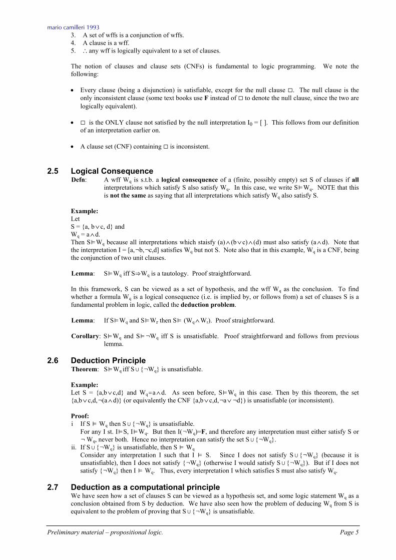
The hypothesis set S can be equivalently viewed as a program, with Wq as a query (or goal statement) to be proved or disproved. The logic interpreter implements a deduction procedure which takes as input S and Wq and attempts to construct a proof that S⊨Wq by refuting S∪{¬Wq}.
Logic Interpreterattempts to prove
thatSÇ Wq
by refutingSá {ÃWq}
Logic ProgramS
Goal StatementWq
Success orFailure
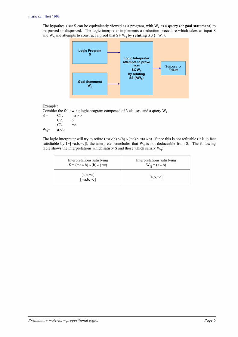
Example: Consider the following logic program composed of 3 clauses, and a query Wq S = C1. ¬a∨b C2. b C3. ¬c Wq= a∧b The logic interpreter will try to refute (¬a∨b)∧(b)∧(¬c)∧¬(a∧b). Since this is not refutable (it is in fact satisfiable by I=[¬a,b,¬c]), the interpreter concludes that Wq is not deduceable from S. The following table shows the interpretations which satisfy S and those which satisfy Wq:
Interpretations satisfying S = (¬a∨b)∧(b)∧(¬c)
Interpretations satisfying Wq = (a∧b)
[a,b,¬c] [¬a,b,¬c] [a,b,¬c]
mario camilleri 1993
Resolution and Horn Clauses Page 7
3 Resolution and Horn Clauses
We have seen that: • Any wff in propositional logic is logically equivalent to a CNF, which is logically equivalent to a set of
clauses.
• The deduction problem is the problem of deciding whether a statement of interest Wq is a logical consequence of a set of clauses S, i.e. S⊨Wq
• But S⊨Wq iff S∪{¬ Wq} is unsatisfiable.
• Hence the deduction and the satisfiability problems are equivalent.
We now show that: • A procedure called resolution, using as inference rule the resolution rule, can be used to refute an
inconsistent CNF.
• Resolution is refutation complete.
• The resolution procedure is non-deterministic.
• One source of non-determinism in the resolution procedure can be eliminated by considering a subset of propositional logic called horn-clause logic.
3.1 Deduction Procedures The logic interpreter needs a procedure for determining the satisfiability of the CNF W=S∪{¬Wq}. One trivial way of doing this would be to have the interpreter enumerate all possible interpretations of W using truth tables, but this brute force approach is unacceptable for 2 main reasons: 1. Truth tables grow exponentially with the size of the base set. 2. In other logics (e.g. functional logic), the anologs of truth tables may not even be finite, and therefore
this approach would not generalize. To overcome these problems, deduction procedures (also called theorem provers) use inference rules to reduce implication to symbolic manipulation and thus avoid brute-force enumeration. The goal is to start with an initial set of formulae and apply inference rules in some order to deduce a particular formula of interest, effectively constructing a proof that it is a logical consequence of the initial set. We are interested in two properties of deduction procedures: 1. Completeness. Given S⇒Wq, will the procedure always be able to demonstarte this using its inference
rules?

mario camilleri 1993
Resolution and Horn Clauses Page 8
2. Complexity. At any point in the procedure there are typically multiple ways of applying the inference rules to deduce new formulae � the choice of which rule to apply next, and to which formula/e to apply it. The deduction procedure uses a search (or selection) strategy to consider each choice in turn. Evidently, the greater the number of choices at each point, the greater the computational cost incurred. Efficient deduction procedures control the amount of choice while maintaining completeness. There are basically two ways choice can be limited in a deduction procedure:
• employing a small set of inference rules, thus reducing the choice of which rule to apply at a particular
step of the proof.
• limiting the set of formulae (candidate set) which need to be considered at each step of the proof.
3.2 Semantic Trees All procedures which improve on the brute-force method are based on the concept of a semantic tree. Let W be a wff of interest (eg. W=S∪{¬Wq}), and its base Bw = {p1,�,pn}, then a semantic tree for W, STw, is a complete binary tree of depth n such that for every interior node at level i, the left edge out of the node is labeled pi and the right edge out of the node is labeled ¬pi. Example: Consider again the logic program S: S = C1. ¬a∨b C2. b C3. ¬c Wq= a∧b and let W= (¬a∨b)∧(b)∧(¬c)∧(¬a∨¬b), the CNF to be refuted in order to prove that S⇒Wq. Then Bw={a,b,c} and STw is as shown. For any node N in the semantic tree, the path from the root to N corresponds to a (possibly partial) interpretation IN. Each root-to-leaf path corresponds to an interpretation. Thus the thick red path shown in the diagram corresponds to the interpretation I=[¬a,b,¬c].
3.3 Failure Nodes Defn: A node N in a semantic tree of a set of clauses W is called a failure node if IN falsifies some
clause in the set, but IM satisfies the set for all ancestor nodes M of N. Example: From the previous example, the CNF to be refuted was W= C1. ¬a∨b C2. b C3. ¬c C4. ¬a∨¬b (≡ ¬(a∧b)) The semantic tree diagram shows the failure nodes, labeled with one of the clauses they falsify. Note that the interpretation corresponding to the thick red path does not falsify any clauses � it satisfies W.
3.4 Failure Trees and Inference Nodes Defn: A failure tree is a semantic tree in which every path terminates in a failure node.
STW
Ãa
Ãb
a
Ãbb b
ÃccC4.ÃaÄÃb C2. b
C3.Ãc
C2. b
STW
Ãa
Ãb
Ãc
a
Ãb
ÃcÃc
b b
ccc Ãcc

mario camilleri 1993
Resolution and Horn Clauses Page 9
Defn: A node N in a failure tree is called an inference node if both its children are failure nodes. Example: Consider the program S and goal formula Wq: S = C1. a∨¬b C2. c∨b C3. ¬c Wq= ¬c∧a Then S∪{¬Wq} is the CNF W = C1. a∨¬b C2. c∨b C3. ¬c C4. c∨¬a (≡ ¬(¬c∧a)) W is refutable (ie. S⇒Wq), and therefore has a failure tree as shown. Note how all paths of the search tree terminate in a failure node (labeled with a clause it falsifies), thus forming a failure tree. Circled nodes in the diagram are inference nodes.
3.5 Properties of Failure Trees 1. A set of clauses (CNF) has a failure tree iff it is unsatisfiable.
Proof straightforward (based on the 1-1 correspondence between interpretations and paths).
2. A set of clauses W has a failure tree of one node iff W contains the null clause □.
The failure tree of one node corresponds to the null interpretation. Since (as seen before) only the null clause can be falsified by the null interpretation, it follows that W must contain the null clause. A similar argument holds in the opposite direction.
3. A failure tree FTw (except the trivial one-node tree) must have at least one inference node.
For if not, then every node must have at least one non-failure descendent, and therefore we could trace a root-to-leaf path. But then FTw would not be a failure tree, for such a path would correspond to an interpretation which satisfies the set W, hence leading to a contradiction.
From the failure tree in the previous diagram, you can see that each inference node has child failure nodes labeled with clauses containing opposite literals. This observation suggests a procedure to establish the inconsistency of a set of clauses.
3.6 The Resolution Principle Consider any two clauses labeling the failure nodes descendent from an inference node in the failure tree diagram, for example, the rightmost inference node is labeled with:
C2. c∨b C3. ¬c
We observe that (c∨b)∧(¬c) ⇒ b. The new clause b is called the RESOLVENT of the two clauses C2 and C3, obtained from the parent clauses C2 and C3 by resolution on the literal c. Because b is a logical consequence of C2 and C3, we can add it as a new clause to the original set W WITHOUT IN ANY WAY AFFECTING THE SATISFIABILITY OF W. Thus, following this resolution step, W will now be
C1. a∨¬b C2. c∨b C3. ¬c C4. c∨¬a C5. b ; resolvent of C2 and C3 wrt c
FTW
Ãa
Ãb
Ãc
a
Ãb
ÃcÃc
b b
ccc
C3.Ãc C4.cÄÃa C3.Ãc C4.cÄÃa C3.Ãc
C1.aÄÃb
C2.cÄb
InferenceNode
mario camilleri 1993
Resolution and Horn Clauses Page 10
We continue applying resolution to the new set by choosing any 2 clauses having complementary literals and 'canceling out' that literal to form a new clause, obtaining
C6. a∨c ;resolvent of C1 and C2 wrt b C7. c ;resolvent of C4 and C6 wrt a C8. □ ;resolvent of C3 and C7 wrt c
Note that the final set of clauses contains the empty clause, and is therefore unsatisfiable. But this set was obtained from the original set W by repeated resolution, and since resolution preserves satisfiability, then the original set W must be inconsistent. Lemma: Let C1 and C2 be two clauses from the CNF W, and let L be a literal st. L is in C1 and ¬L is in
C2. Then the clause CR = C1\L ∪ C2\¬L, called the resolvent clause, is a logical consequence of W. Moreover, W ≡ W ∪ {CR}.
Example:
C1= a∨b∨c C2= d∨¬c∨¬a CR= ¬c∨b∨c∨d
Note that in this example, the clauses are resolved wrt the literal a. We could just as easily have resolved wrt the literal c. Defn: The resolution closure W* of a set of clauses W is the closure of the set W under the operation
of resolution.
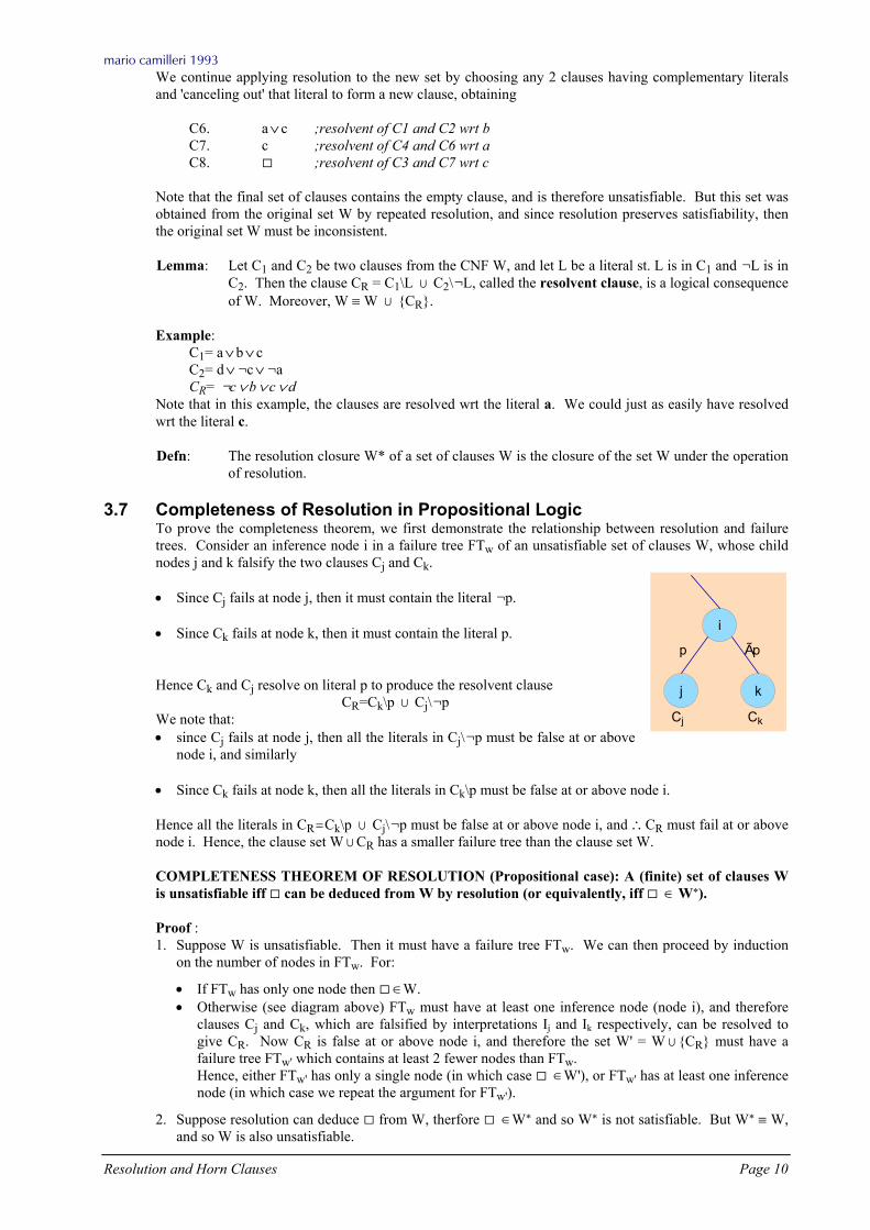
3.7 Completeness of Resolution in Propositional Logic To prove the completeness theorem, we first demonstrate the relationship between resolution and failure trees. Consider an inference node i in a failure tree FTw of an unsatisfiable set of clauses W, whose child nodes j and k falsify the two clauses Cj and Ck. • Since Cj fails at node j, then it must contain the literal ¬p.
• Since Ck fails at node k, then it must contain the literal p.
Hence Ck and Cj resolve on literal p to produce the resolvent clause
CR=Ck\p ∪ Cj\¬p We note that: • since Cj fails at node j, then all the literals in Cj\¬p must be false at or above
node i, and similarly
• Since Ck fails at node k, then all the literals in Ck\p must be false at or above node i.
Hence all the literals in CR=Ck\p ∪ Cj\¬p must be false at or above node i, and ∴ CR must fail at or above node i. Hence, the clause set W∪CR has a smaller failure tree than the clause set W. COMPLETENESS THEOREM OF RESOLUTION (Propositional case): A (finite) set of clauses W is unsatisfiable iff □ can be deduced from W by resolution (or equivalently, iff □ ∈ W¾). Proof : 1. Suppose W is unsatisfiable. Then it must have a failure tree FTw. We can then proceed by induction
on the number of nodes in FTw. For:
• If FTw has only one node then □∈W. • Otherwise (see diagram above) FTw must have at least one inference node (node i), and therefore
clauses Cj and Ck, which are falsified by interpretations Ij and Ik respectively, can be resolved to give CR. Now CR is false at or above node i, and therefore the set W' = W∪{CR} must have a failure tree FTw' which contains at least 2 fewer nodes than FTw. Hence, either FTw' has only a single node (in which case □ ∈W'), or FTw' has at least one inference node (in which case we repeat the argument for FTw').
2. Suppose resolution can deduce □ from W, therfore □ ∈W¾ and so W¾ is not satisfiable. But W¾ ≡ W, and so W is also unsatisfiable.
i
j k
Cj Ck
p Ãp

mario camilleri 1993
Resolution and Horn Clauses Page 11
3.8 Inconsistency proofs based on Resolution The resolution method, devloped in 1965 by J. Robinson1 has become popular in automatic theorem proving because it is simple to implement, having only a single inference rule (the resolution rule). Thus, resolution eliminates one source of non-determinism � that of which rule to apply next in the course of constructing a proof. The resolution rule is able to establish the inconsistency of any set of clauses W as follows:
Procedure REFUTE(W:CNF) 1 While □ ∉ W 2 Select C1,C2 ∈W and an atom p, such that p∈C1 and ¬p∈C2 3 Compute CR, the resolvent of C1 and C2 4 Add CR to W
We note that: • The completeness theorem quarantees that REFUTE will terminate, and deduce □, iff W is inconsistent
(unsatisfiable).
• If W does not contain any resolvable clauses (and does not contain □) then it is consistent (satisfiable), and we can have REFUTE test for this in step 2 and halt with SUCCESS. But in general, REFUTE may not halt if W is consistent. For example, consider the consistent set
W = {a, ¬a ∨ b}
REFUTE will not halt for W, generating b infinitely.
3.9 Non-Determinism in Resolution Refutations There are 2 sources of non-determinism in REFUTE, both in step 2: 1. deciding which two clauses to resolve next, and
2. deciding which literal to resolve upon (since there may be many literals which are positive in one clause and negative in the other).
3.10 Horn-Clause Logic We can completely eliminate Type 2 choices by restricting our programs to a subset of logic called Horn-Clause logic. A Horn clause is a clause with at most 1 positive literal. The following cases may arise: 1. The empty clause □.
As seen, this clause represents F since no interpretation can satisfy it.
2. A clause with exactly one positive literal (a positive horn clause).
• A clause with no negative literals, for example C=p (a UNIT clause). In this case an interpretation I⊨C iff I(p)=T. Thus such a clause represents an assertion.
• A clause with negative literals, for example the clause C=p∨¬n1∨¬n2∨ ... ∨¬nn. Suppose that an interpretation I satisfies all of n1 � nn. Then ¬n1 � ¬nn are all false, and therefore for C to be satisfied, I⊨p. Thus C ≡ (n1∧n2∧ ... ∧nn) ⇒ p, ie. n1..nn may be considered premises of which p is the conclusion.
3. A clause with only negative literals (a negative horn clause).
For example C = ¬n1∨¬n2∨ ... ∨¬nn.
In this case C ≡ ¬(n1∧n2∧ ... ∧nn), the negation of a CNF of unit clauses. We will see later that we can use the CNF as the goal statement requiring proof.
1 Robinson,J.A. (1965) A Machine-Oriented Logic Based on the Resolution Principle, in JACM Vol.12 No.1 January 1965, pp.23-
41. Iff anyone is interested, just ask me for a copy � be warned however that it treats the first-order case, not the propositional case.

mario camilleri 1993
Resolution and Horn Clauses Page 12
NOTE that while clauses and CNFs can represent any wff, Horn clauses cannot, so Horn-Clause logic is less expressive than full propositional logic. What we gain by using Horn clauses is the important property that a clause cannot have more than 1 positive literal, thus eliminating Type 2 choices from our REFUTE procedure. Lemma: Horn clauses are closed under resolution. Since every horn clause has at most one positive literal, and since resolution �cancels� a
positive with a negative literal, the resolvent of two horn clauses will have at most only one positive literal, and therefore is itself a horn clause.
Lemma: Positive horn clauses are closed under resolution. The resolvent of two horn clauses must have exactly one positive literal, and is therefore itself
a positive horn clause. The distinction between positive and negative horn clauses is crucial. Because positive horn clauses are closed under resolution, □ can never be derived from a set of positive horn clauses. Such a set is thus consistent � a model can be constructed by assigning T to all positive literals in the set.
3.11 Horn-Clause Logic Programs Consider a set of positive horn-clauses, S. Since all clauses in S are positive, resolution will never generate □ from this set, and so S is satisfiable under some interpretation I. Since a set of clauses is a CNF (a CONJUNCTION of clauses), then ALL clauses in S are TRUE under I. Hence S represents a body of �knowledge� often called a KNOWLEDGE BASE. Suppose we wish to know whether a WFF Wq (called a query) logically follows from S. Then, • S⊨Wq iff S∪{¬Wq} is unsatifiable, by deduction principle;
• iff S∪{¬Wq}⊨□, by completeness of resolution.
Since we are using horn-clause resolution, this places some constraints on the form of Wq. Specifically, we want ¬Wq to be a negative horn clause. Thus Wq must be a conjunction of positive literals. Example: Wq = a∧b∧c so that ¬Wq = N0 = ¬a∨¬b∨¬c so S ∪ {N0} is still a CNF of horn clauses with a single negative horn clause (i.e. N0). N0 is thus a negative horn clause (a negation of the original query), and is usually called the GOAL. Thus, a horn logic program is made up of two objects:
INTERPRETERUses resolutionto derive Ð from
S á {N0}
SKNOWLEDGE BASEA set of positive Horn
clauses
N0GOAL STATEMENT
A negative Hornclause
Ð
3.12 Exercises 1. Consider the CNF :
S = C1 h C2 ¬h∨p∨q C3 ¬p∨c C4 ¬q∨c
Using resolution refutation, show that S⊨c.
mario camilleri 1993
Resolution and Horn Clauses Page 13
2. Let S be a set of clauses, and let CR be the resolvent of 2 clauses in S. Show that
S ≡ S∪{CR} 3. Use semantic trees to derive an upper bound on the minimum number of resolution steps needed to
deduce □ from an inconsistent set S. Hint: consider |BS|.
4. We have shown that a set of positive horn clauses is satisfiable, because resolution can never derive □ from such a set. Show that any set of horn clauses each of which contains at least one negative literal (i.e. the set does not contain unit clauses) must also be satisfiable.
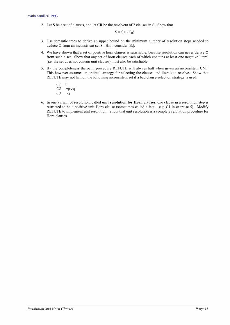
5. By the completeness theroem, procedure REFUTE will always halt when given an inconsistent CNF. This however assumes an optimal strategy for selecting the clauses and literals to resolve. Show that REFUTE may not halt on the following inconsistent set if a bad clause-selection strategy is used:
C1 P C2 ¬p∨q C3 ¬q
6. In one variant of resolution, called unit resolution for Horn clauses, one clause in a resolution step is
restricted to be a positive unit Horn clause (sometimes called a fact � e.g. C1 in exercise 5). Modify REFUTE to implement unit resolution. Show that unit resolution is a complete refutation procedure for Horn clauses.

mario camilleri 1993
The Language Proplog Page 14
4 The Language Proplog
We have seen that: • The Resolution deduction procedure uses only a single inference rule � the resolution rule.
• The Resolution procedure attempts to refute a set of clauses by deducing □ using the resolution rule.
• Resolution is refutation complete � the closure W¾ of an inconsistent CNF W under Resolution must contain □. Proof by induction on number of nodes in failure tree FTW.
• The Resolution procedure has 2 sources of non-determinism � deciding which two clauses to resolve next, and deciding which literals to resolve upon.
• The second source of non-determinism can be eliminated by restricting resolution to Horn clauses � clauses with at most one positive literal.
We now: • Adopt a new syntax for Horn-clause, and show their correspondence to CFGs.
• Describe a propositional-logic programming language called PropLog.
• Describe an efficient refutation procedure for PropLog based on SLD-resolution.
• Show how the choice of a search-strategy can affect the completeness of the refutation procedure.
4.1 Some Syntactic Sugar Let us adopt the convention of writing the Horn-clause
¬a∨¬b∨¬c∨d as
d :- a,b,c. Note that this is purely a syntactic modification � the semantics of the clause have not changed. This new notation gives rise to an interesting analogy with productions in context free grammars.
4.2 Horn Clauses and Rewriting Rules A Horn clause can be considered as a rewriting rule (or production), and a set of Horn clauses can be viewed as a context-free grammar whose symbols are the propositional symbols together with the distinguished symbol □ � the start symbol2. For example, consider this set of Horn clauses:
2 For a proof that the satisfiability problem on sets of Horn clauses is equivalent to the problem of deriving ε from a CFG, see
Dowling and Gallier (1984) A Linear-time Algorithm for testing the Satisfiability of Propositional Horn Formulae, in Journal of Logic Programming 1984:3 pp.267-284
mario camilleri 1993
The Language Proplog Page 15
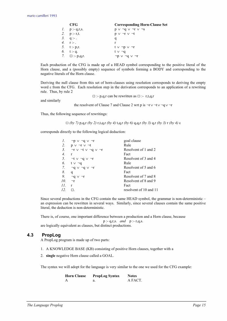
CFG Corresponding Horn-Clause Set 1. p :- q,r,s. p ∨ ¬q ∨ ¬r ∨ ¬s 2. p :- r,t. p ∨ ¬r ∨ ¬t 3. q :- . q 4. r :- . r 5. t :- p,r. t ∨ ¬p ∨ ¬r 6. t :- q. t ∨ ¬q 7. □ :- p,q,r. ¬p ∨ ¬q ∨ ¬r
Each production of the CFG is made up of a HEAD symbol corresponding to the positive literal of the Horn clause, and a (possibly empty) sequence of symbols forming a BODY and corresponding to the negative literals of the Horn clause. Deriving the null clause from this set of horn-clauses using resolution corresponds to deriving the empty word ε from the CFG. Each resolution step in the derivation corresponds to an application of a rewriting rule. Thus, by rule 2
□ :- p,q,r can be rewritten as □ :- r,t,q,r and similarly
the resolvent of Clause 7 and Clause 2 wrt p is ¬r∨¬t∨¬q∨¬r Thus, the following sequence of rewritings:
□ (by 7) p,q,r (by 2) r,t,q,r (by 4) t,q,r (by 6) q,q,r (by 3) q,r (by 3) r (by 4) ε corresponds directly to the following logical deduction:
1. ¬p ∨ ¬q ∨ ¬r goal clause 2. p ∨ ¬r ∨ ¬t Rule 3. ¬r ∨ ¬t ∨ ¬q ∨ ¬r Resolvent of 1 and 2 4. r Fact 5. ¬t ∨ ¬q ∨ ¬r Resolvent of 3 and 4 6. t ∨ ¬q Rule 7. ¬q ∨ ¬q ∨ ¬r Resolvent of 5 and 6 8. q Fact 9. ¬q ∨ ¬r Resolvent of 7 and 8
10. ¬r Resolvent of 8 and 9 11. r Fact 12. □. resolvent of 10 and 11
Since several productions in the CFG contain the same HEAD symbol, the grammar is non-deterministic � an expression can be rewritten in several ways. Similarly, since several clauses contain the same positive literal, the deduction is non-deterministic. There is, of course, one important difference between a production and a Horn clause, because
p :- q,r,s. and p :- r,q,s. are logically equivalent as clauses, but distinct productions.
4.3 PropLog A PropLog program is made up of two parts: 1. A KNOWLEDGE BASE (KB) consisting of positive Horn clauses, together with a
2. single negative Horn clause called a GOAL.
The syntax we will adopt for the language is very similar to the one we used for the CFG example:
Horn Clause PropLog Syntax Notes A a. A FACT.
mario camilleri 1993
The Language Proplog Page 16
a∨¬b∨¬c a :- b,c. A RULE. The positive literal is called the HEAD of the rule, the conjunction of negative literals is called the BODY of the rule.
¬b∨¬c b,c ? A QUERY/GOAL. There is precisely ONE query in every PropLog program. An alternative syntax would be: :- b,c.
The difference between a QUERY and a GOAL is that the QUERY is the statement to be proved, and is a conjunction of positive literals. The GOAL is the negation of the query, and is a negative horn clause. Nevertheless, the two terms are frequently used interchangeably. Example PropLog program:
q. t.
; 2 facts
p :- q,r. r :- q,s. r :- q,t.
; 3 rules.
P? ; QUERY (or initial GOAL)
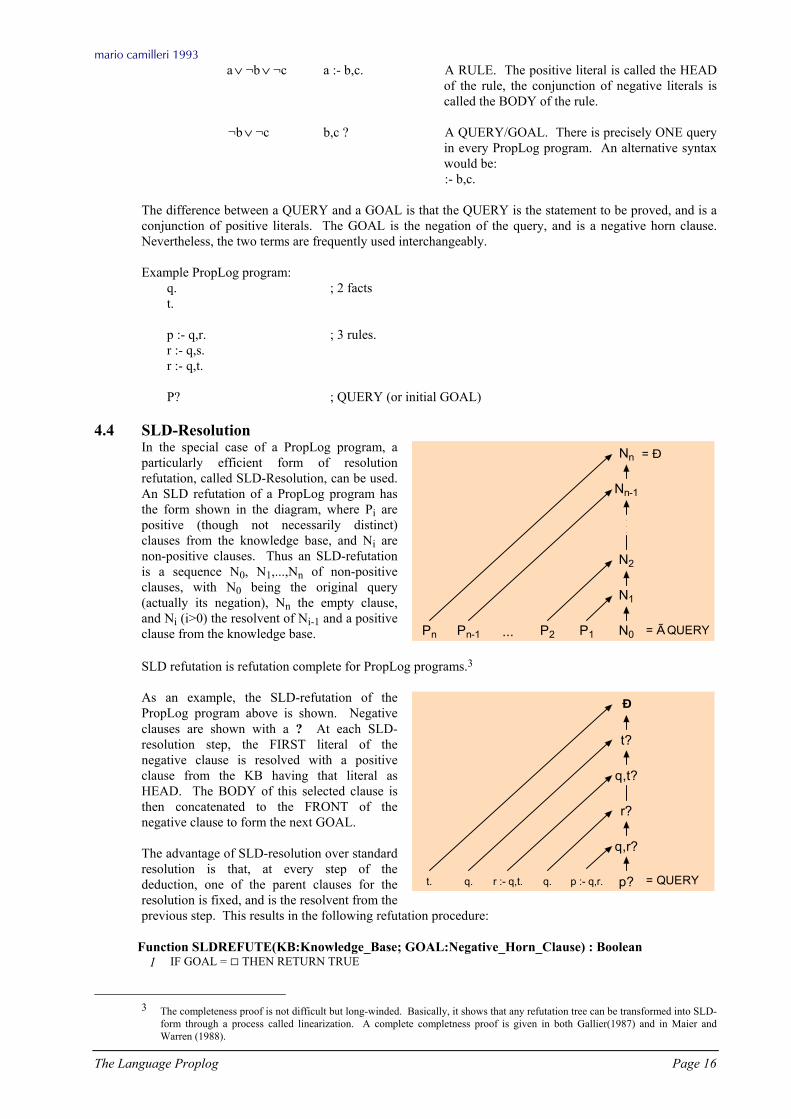
4.4 SLD-Resolution In the special case of a PropLog program, a particularly efficient form of resolution refutation, called SLD-Resolution, can be used. An SLD refutation of a PropLog program has the form shown in the diagram, where Pi are positive (though not necessarily distinct) clauses from the knowledge base, and Ni are non-positive clauses. Thus an SLD-refutation is a sequence N0, N1,...,Nn of non-positive clauses, with N0 being the original query (actually its negation), Nn the empty clause, and Ni (i>0) the resolvent of Ni-1 and a positive clause from the knowledge base. SLD refutation is refutation complete for PropLog programs.3 As an example, the SLD-refutation of the PropLog program above is shown. Negative clauses are shown with a ? At each SLD-resolution step, the FIRST literal of the negative clause is resolved with a positive clause from the KB having that literal as HEAD. The BODY of this selected clause is then concatenated to the FRONT of the negative clause to form the next GOAL. The advantage of SLD-resolution over standard resolution is that, at every step of the deduction, one of the parent clauses for the resolution is fixed, and is the resolvent from the previous step. This results in the following refutation procedure:
Function SLDREFUTE(KB:Knowledge_Base; GOAL:Negative_Horn_Clause) : Boolean 1 IF GOAL = □ THEN RETURN TRUE
3 The completeness proof is not difficult but long-winded. Basically, it shows that any refutation tree can be transformed into SLD-
form through a process called linearization. A complete completness proof is given in both Gallier(1987) and in Maier and Warren (1988).
Pn Pn-1 P2 P1 N0
N1
N2
Nn-1
Nn
...
= Ð
= Ã QUERY
.
.
.
t. q. q. p :- q,r. p?
q,r?
r?
t?
Ð
r :- q,t. = QUERY
q,t?
mario camilleri 1993
The Language Proplog Page 17
2 Select the atom p = FIRST(GOAL) 3 IF ∃ C∈KB st (p=HEAD(C)) AND SLDREFUTE(KB,BODY(C) + REST(GOAL)) THEN 4 RETURN TRUE 5 ELSE RETURN FALSE
6 WRITELN(SLDREFUTE(KB,¬QUERY))
Step 6 of the algorithm represents the 'main program' � the initial call to the refutation function passes the original query as the goal.
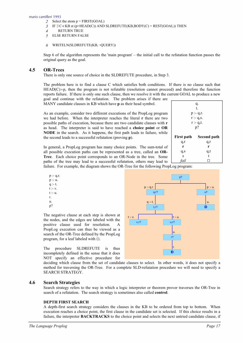
4.5 OR-Trees There is only one source of choice in the SLDREFUTE procedure, in Step 3. The problem here is to find a clause C which satisfies both conditions. If there is no clause such that HEAD(C)=p, then the program is not refutable (resolution cannot proceed) and therefore the function reports failure. If there is only one such clause, then we resolve it with the current GOAL to produce a new goal and continue with the refutation. The problem arises if there are MANY candidate clauses in KB which have p as their head symbol. As an example, consider two different executions of the PropLog program we had before. When the interpreter reaches the literal r there are two possible paths of execution, because there are two candidate clauses with r as head. The interpreter is said to have reached a choice point or OR NODE in the search. As it happens, the first path leads to failure, while the second leads to a successful refutation (proving p). In general, a PropLog program has many choice points. The sum-total of all possible execution paths can be represented as a tree, called an OR-Tree. Each choice point corresponds to an OR-Node in the tree. Some paths of the tree may lead to a successful refutation, others may lead to failure. For example, the diagram shows the OR-Tree for the following PropLog program:
p :- q,r. p :- u. q :- t. t :- v. t :- u. r. u. p?
The negative clause at each step is shown at the nodes, and the edges are labeled with the positive clause used for resolution. A PropLog execution can thus be viewed as a search of the OR-Tree defined by the PropLog program, for a leaf labeled with □. The procedure SLDREFUTE is thus incompletely defined in the sense that it does NOT specify an effective procedure for deciding which clause from the set of candidate clauses to select. In other words, it does not specify a method for traversing the OR-Tree. For a complete SLD-refutation procedure we will need to specify a SEARCH STRATEGY.
4.6 Search Strategies Search strategy refers to the way in which a logic interpreter or theorem prover traverses the OR-Tree in search of a refutation. The search strategy is sometimes also called control. DEPTH FIRST SEARCH A depth-first search strategy considers the clauses in the KB to be ordered from top to bottom. When execution reaches a choice point, the first clause in the candidate set is selected. If this choice results in a failure, the interpreter BACKTRACKS to the choice point and selects the next untried candidate clause, if
q. t.
p :- q,r. r :- q,s. r :- q,t.
p?
First path Second path q,r r
q,s s
fail
q,r r
q,t t □
p?
q,r? u?
t,r? Ð
v,r? u,r?
r?
Ð
p :- q,r. p :- u.
q :- t. u.
t :- v. t :- u.
u.
r.

mario camilleri 1993
The Language Proplog Page 18
any. If all clauses at a choice point lead to failure, further backtracking to the previous choice point (if any) is required. As a tree-traversal, the depth-first strategy corresponds to a pre-order search for a leaf labeled with a □. A problem arises with this search strategy because an OR-tree may have infinitely-long paths as well as paths which terminate in □ (i.e. paths leading to a refutation). If the infinite path is encountered first, the algorithm will fail to terminate even though the PropLog program is refutable. The following program is not refutable if the refutation startegy employs a depth-first search:
a :- c,b. a :- d,b. c :- a. d. b. a?
Since a depth-first strategy may fail to refute a refutable program, it is not complete. It does have its advantages, however � it is easy and compact to implement and is used in most Prolog implementations. BREADTH-FIRST SEARCH The breadth-first search traverses the OR-tree level-by-level, considering all paths simultaneously to some given depth. This guarantees that breadth-first search will always find □ if the program is refutable. It is however expensive to implement. Note that if the program is NOT refutable, then it may still not halt.
4.7 The Closed-World Assumption and Negation by Failure In restricting our knowledge-base to definite (i.e. positive) clauses, we have effectively restricted ourselves to stating what is TRUE, but not what is FALSE. Suppose we wanted to state that b is false. We cannot state this fact in the KB, because the knowledge base of a PropLog program is a set of positive Horn clauses. One way to overcome this problem is to adopt the closed-world assumption (CWA). This assumes that: 1. All facts and rules in the knowledge-base are true.
2. ONLY the facts and rules in the knowledge-base are true.
Thus, under CWA, anything not provable from the knowledge base is by default false. This leads to an interesting semantics for negation called NEGATION BY FAILURE, different from clasical negation. Because of the CWA, we assume that if a is not provable, then it is false.
a?
c,b? d,b?
a,b? b?
c,b? d,b? Ð
b?
� Ð
a :- c,b. a :- d,b.
c :- a. d.
b.a :- c,b. a :- d,b.
c :- a.
d.
b.

mario camilleri 1993
Datalog Page 19
5 Datalog
We have described a simple language (PropLog) based on propositional logic. We saw that such a language has two components: • a LOGIC component, and
• a CONTROL component (or STRATEGY) which specifies the order in which the computation is to proceed (the traversal of the search tree).
PropLog used SLD resolution on Horn clauses with a depth-first search strategy to refute a goal statement (thereby proving the original query). We now: describe an enhanced language called DataLog based on predicate logic. DataLog uses predicates instead of propositions to represent relations.
5.1 DataLog In this chapter we enhance our PropLog language by adding relations and logic variables. The new language, called DataLog, is a subset of Prolog sufficiently powerful to act as a database query language4 (hence its name).
5.2 Relations Conceptually, a relation R is a table with n≥0 columns called attributes, and a (possibly infinite) set of rows. n is stb the arity of R. A tuple (a1,�,an) is IN relation R if, for all i, ai appears in column i of some row of R. Consider a relation married:
married Husband Wife anthony ann
bob betty bill bella carl claire
Relation married is of arity 2 (sometimes we write this as married/2). Tuples (anthony,ann) and (bill,bella) are in relation married, but tuples (ann,anthony) and (tom,tina) are not.
5.3 Predicates We can represent a relation as a set of facts:
married(anthony,ann).
4 For a very readable article on the impact of logic programming on databases see: Grant,J. and Minker,J. (1992) The Impact of
Logic Programming on Databases, in CACM March 1992 pp.66-81. This issue of the CACM was dedicated to Logic Programming.

mario camilleri 1993
Datalog Page 20
married(bob,betty). married(bill,bella). married(carl,claire).
These facts list all tuples in relation married. married is called a predicate of arity 2. In representing a relation in this way, we have lost all information on attribute names, so we must be careful to preserve the ordering of the predicate's arguments to reflect the original relation.
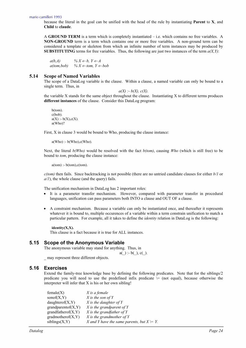
5.4 Family relations Consider the following family tree which we wish to represent as a knowledge base using predicates to model relations. There are various ways to represent the family tree. We will use the following two predicates:
married(X,Y) X is the husband, Y is the wife. motherof(X,Y) X is the mother, Y is the child.
We can then represent the family tree using the following knowledge base of facts:
ann+
anthony
betty+
bobbert
bella+
bill
carl+
clairecory candy
claude+
carol
deborahdominic
+daphne
donna
married(anthony,ann). married(bob,betty). married(bill,bella). married(carl,claire). married(claude,carol). married(dominic,daphne).
motherof(ann,betty). motherof(ann,bert). motherof(ann,bella). motherof(betty,carl). motherof(betty,cory). motherof(bella,candy). motherof(bella,claude). motherof(claire,deborah). motherof(carol,dominic). motherof(carol,donna).
5.5 Queries and Unification Given the above knowledgebase, we can ask queries such as:
married(bob,betty)? motherof(ann,donna)?
The first query succeeds because it UNIFIES (matches) with the second clause of the married predicate. The second query fails because it does not unify with any of the clauses in the motherof predicate.
5.6 Queries and logic Variables Both of the above two queries could easily have been handled by the PropLog interpreter, since in either case the answer is a YES (success) or a NO (failure).

mario camilleri 1993
Datalog Page 21
More usefully, we can ask queries involving unknowns. Unknowns are represented by variables (syntactically, symbols starting with an uppercase letter), such as:
married(carl,X)?
This query effectively asks whether
∃X s.t. married(carl,X) The logic interpreter succeeds in demonstrating married(carl,X) because this unifies with the fourth clause of the married predicate. This unification causes the free variable X to be INSTANTIATED to claire. Besides succeeding, this query also produces the answer that
X=claire. Consider the query:
motherof(betty,X)? The interpreter will first succeed in unifying the goal motherof(betty,X) with the 4th clause of the motherof predicate, by instantiating X to carl. This will produce the answer X=carl. Following backtracking, the goal will also unify with the 5th clause, generating the answer X=cory. Further backtracking results in failure.
5.7 Rules Suppose we wanted to add facts about husbands to our knowledgebase. One way of doing this would be to add 6 clauses for a predicate isahusband/1, for example:
isahusband(anthony). isahusband(bob). ...
However, we note that husbands always appear as the first argument of a clause for the married/2 predicate. Thus, we can write a single rule:
isahusband(X) :- married(X,Y). This rule effectively states that, for all X such that the relation married(X,Y) holds, X is a husband. Note how the rule is like a TEMPLATE from which facts can be generated. In this rule, the variable Y simply represents ANYBODY � we're not really interested in the identity of X's wife. For clarity, in such situations we may use the anonymous variable _, and write:
isahusband(X) :- married(X,_).
5.8 Commutativity The married/2 predicate presupposes a certain ordering of its argument. The rule isahusband relies on this ordering. We could define a predicate aremarried/2 which succeeds if two people are married, irrespective of the ordering of its arguments:
aremarried(X,Y) :- married(X,Y). aremarried(X,Y) :- married(Y,X).
Thus, aremarried(anthony,ann)? %succeeds by first clause of rule aremarried(ann,anthony)? %succeeds by second clause of rule
5.9 Transitivity Consider the problem of determining whether X is the father of Z. Assuming a very simple world (sometimes called the simple-world assumption, or SWA), we can do this by noting that, if X is married to Y, and Y is the mother of Z, then X is the father of Z. Thus:
fatherof(Father,Child) :- married(Father,W), motherof(W,Child).
mario camilleri 1993
Datalog Page 22
Having defined fatherof, we can now define a general rule for parentof/2:
parentof(Parent,Child) :- motherof(Parent,Child). parentof(Parent,Child) :- fatherof(Parent,Child).
5.10 Mixing Facts and Rules Suppose we want to add a male/1 predicate to the knowledgebase. We note that all husbands are males, but not all males are husbands. We can define the predicate male/1 as follows:
male(bert). male(X) :- married(X,_).
Here we say that X is a male either if X is bert, or if X is the first argument of some clause for the married/2 predicate.
5.11 Recursive Rules The following predicate defines the ancestorof relation recursively:
ancestorof(A,Someone) :- parentof(A,Someone). ancestorof(A,Someone) :- parentof(A,X), ancestorof(X,Someone).
Care must be taken when defining recursive rules not to create infinite loops. This would have happened if the second clause in ancestor/2 were made left-recursive, as follows:
% Loops infinitely because of left recursion. ancestorof(A,Someone) :- parentof(A,Someone). ancestorof(A,Someone) :- ancestorof(X,Someone), parentof(A,X).
This rule would succeed in finding all ancestors, but would then enter an infinte loop.
5.12 Components of Datalog • A DataLog knowledge base (or DATABASE) is a sequence of POSITIVE (or DEFINITE) CLAUSES.
• A POSITIVE CLAUSE is made up of a HEAD and a BODY. The BODY consists of a (possibly empty) sequence of GOALS.
• If the BODY of the CLAUSE is not empty, the clause is called a RULE, and is written as
a :- b,c,d. where a is the HEAD and b,c and d the GOALS making up the body of the clause. This is logically
equivalent to b∧c∧d ⇒ a
The HEAD and GOALS of a CLAUSE are called LITERALS. • If the BODY of the clause is the empty sequence, then the clause is called a FACT (or UNIT
CLAUSE), and is simply written as
a. • A DataLog program is made up of a DataLog knowledge base together with a single NEGATIVE
CLAUSE called a GOAL STATEMENT (or QUERY) and having the form
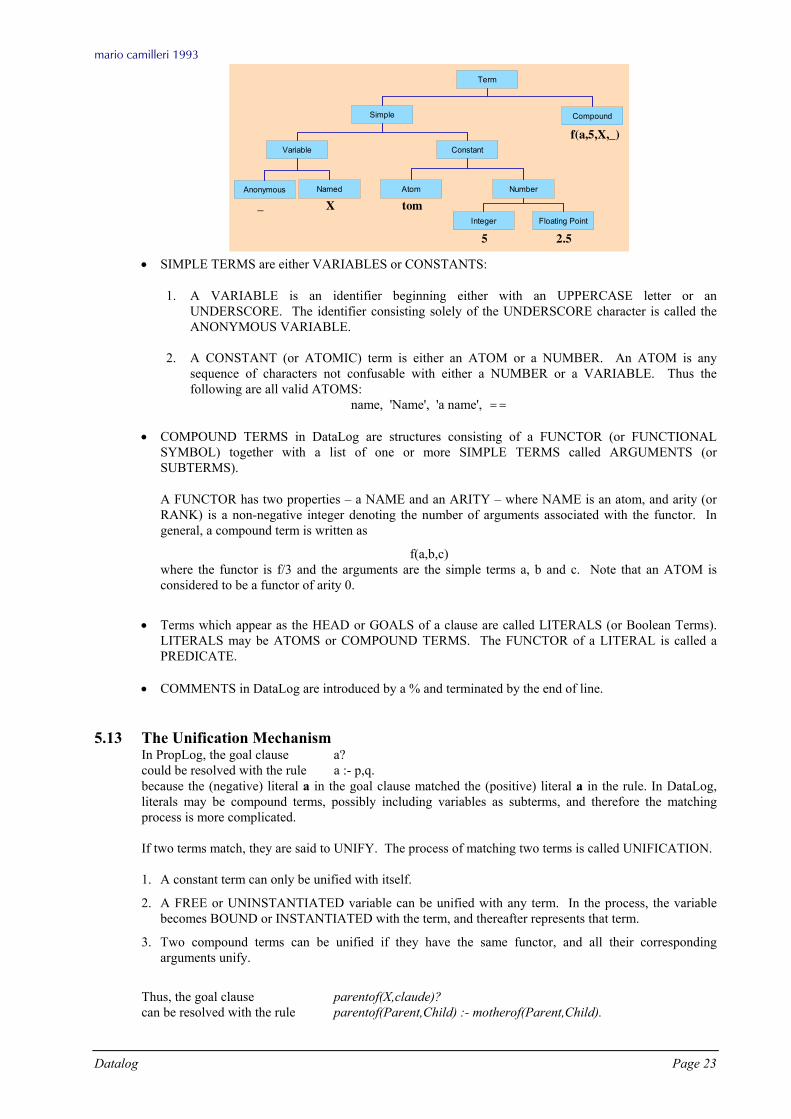
a,b,c ? • A TERM may be SIMPLE or COMPOUND:
mario camilleri 1993
Datalog Page 23
Term
Simple Compound
Variable Constant
Atom Number
Integer Floating Point
Anonymous Named
_ X tom
5 2.5
f(a,5,X,_)
• SIMPLE TERMS are either VARIABLES or CONSTANTS:
1. A VARIABLE is an identifier beginning either with an UPPERCASE letter or an UNDERSCORE. The identifier consisting solely of the UNDERSCORE character is called the ANONYMOUS VARIABLE.
2. A CONSTANT (or ATOMIC) term is either an ATOM or a NUMBER. An ATOM is any
sequence of characters not confusable with either a NUMBER or a VARIABLE. Thus the following are all valid ATOMS:
name, 'Name', 'a name', == • COMPOUND TERMS in DataLog are structures consisting of a FUNCTOR (or FUNCTIONAL
SYMBOL) together with a list of one or more SIMPLE TERMS called ARGUMENTS (or SUBTERMS).
A FUNCTOR has two properties � a NAME and an ARITY � where NAME is an atom, and arity (or RANK) is a non-negative integer denoting the number of arguments associated with the functor. In general, a compound term is written as
f(a,b,c) where the functor is f/3 and the arguments are the simple terms a, b and c. Note that an ATOM is considered to be a functor of arity 0.
• Terms which appear as the HEAD or GOALS of a clause are called LITERALS (or Boolean Terms).
LITERALS may be ATOMS or COMPOUND TERMS. The FUNCTOR of a LITERAL is called a PREDICATE.
• COMMENTS in DataLog are introduced by a % and terminated by the end of line.
5.13 The Unification Mechanism In PropLog, the goal clause a? could be resolved with the rule a :- p,q. because the (negative) literal a in the goal clause matched the (positive) literal a in the rule. In DataLog, literals may be compound terms, possibly including variables as subterms, and therefore the matching process is more complicated. If two terms match, they are said to UNIFY. The process of matching two terms is called UNIFICATION. 1. A constant term can only be unified with itself.
2. A FREE or UNINSTANTIATED variable can be unified with any term. In the process, the variable becomes BOUND or INSTANTIATED with the term, and thereafter represents that term.
3. Two compound terms can be unified if they have the same functor, and all their corresponding arguments unify.
Thus, the goal clause parentof(X,claude)? can be resolved with the rule parentof(Parent,Child) :- motherof(Parent,Child).
mario camilleri 1993
Datalog Page 24
because the literal in the goal can be unified with the head of the rule by instantiating Parent to X, and Child to claude. A GROUND TERM is a term which is completely instantiated � i.e. which contains no free variables. A NON-GROUND term is a term which contains one or more free variables. A non-ground term can be considered a template or skeleton from which an infinite number of term instances may be produced by SUBSTITUTING terms for free variables. Thus, the following are just two instances of the term a(X,Y): a(b,A) % X ← b, Y ← A a(tom,bob) % X ← tom, Y ← bob
5.14 Scope of Named Variables The scope of a DataLog variable is the clause. Within a clause, a named variable can only be bound to a single term. Thus, in
a(X) :- b(X), c(X). the variable X stands for the same object throughout the clause. Instantiating X to different terms produces different instances of the clause. Consider this DataLog program:
b(tom). c(bob). a(X) :- b(X),c(X). a(Who)?
First, X in clause 3 would be bound to Who, producing the clause instance:
a(Who) :- b(Who),c(Who).
Next, the literal b(Who) would be resolved with the fact b(tom), causing Who (which is still free) to be bound to tom, producing the clause instance:
a(tom) :- b(tom),c(tom).
c(tom) then fails. Since backtracking is not possible (there are no untried candidate clauses for either b/1 or a/1), the whole clause (and the query) fails. The unification mechanism in DataLog has 2 important roles: • It is a parameter transfer mechanism. However, compared with parameter transfer in procedural
languages, unification can pass parameters both INTO a clause and OUT OF a clause.
• A constraint mechanism. Because a variable can only be instantiated once, and thereafter it represents whatever it is bound to, multiple occurences of a variable within a term constrain unification to match a particular pattern. For example, all it takes to define the identity relation in DataLog is the following:
identity(X,X). This clause is a fact because it is true for ALL instances.
5.15 Scope of the Anonymous Variable The anonymous variable may stand for anything. Thus, in
a(_) :- b(_), c(_). _ may represent three different objects.
5.16 Exercises Extend the family-tree knowledge base by defining the following predicates. Note that for the siblings/2 predicate you will need to use the predefined infix predicate \= (not equal), because otherwise the interpreter will infer that X is his or her own sibling!
female(X) X is a female sonof(X,Y) X is the son of Y daughterof(X,Y) X is the daughter of Y grandparentof(X,Y) X is the grandparent of Y grandfatherof(X,Y) X is the grandfather of Y gradmotherof(X,Y) X is the grandmother of Y siblings(X,Y) X and Y have the same parents, but X \= Y.
mario camilleri 1993
Datalog Page 25
brotherof(X,Y) brother of X is Y sisterof(X,Y) sister of X is Y auntof(X,Y) X is the aunt of Y uncleof(X,Y) X is the uncle of Y
You should write the knowledgebase using any text editor and save it under the filename family (it's best if you don't include an extension). You should then run the Prolog86+ interpreter:
F:\APPS\LNG\PLG86\PROLOG Prolog86+ defaults to reading from drive A:. From the : prompt, load the knowledgebase
load family? If the knowledgebase loads successfully, Prolog86+ should answer ** yes and return you to the : prompt. Otherwise, an error message will appear. You can edit a loaded file using:
em family? This will invoke the text editor with the file family (currently the public domain editor boxer.exe is used). Edit the file, save it, and quit the editor. Prolog86+ will then attempt to reload the knowledgebase. Once the knwoledgebase loads successfully and you are at the : prompt, you can issue queries. A query is terminated by a ? and may continue on multiple lines � so, if you press ENTER in the middle of a query by mistake, DON'T retype everything again, just continue on the next line. Remember that only variables can start with a capital letter � everything else must start with a lowercase letter. You can quit Prolog86+ by typing
halt? NOTE that if you use the older Prolog86 instead of Prolog86+, the inequality operator is /=.
mario camilleri 1993
Prolog Page 26
6 Prolog
We have described a simple logic language called DATALOG based on predicate calculus. DataLog allowed us to express statements about relations over the domain of simple atomic terms. We now extend DataLog by allowing relations over the domain of compound terms � terms which can represent whole data structures. This new language is Prolog. Just as DataLog was based on predicate logic, so Prolog is based on functional logic.
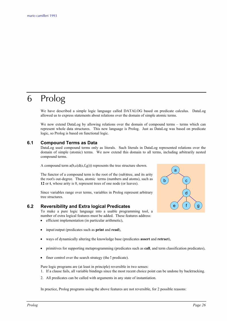
6.1 Compound Terms as Data DataLog used compound terms only as literals. Such literals in DataLog represented relations over the domain of simple (atomic) terms. We now extend this domain to all terms, including arbitrarily nested compound terms. A compound term a(b,c(d(e,f,g))) represents the tree structure shown. The functor of a compound term is the root of the (sub)tree, and its arity the root's out-degree. Thus, atomic terms (numbers and atoms), such as 12 or t, whose arity is 0, represent trees of one node (or leaves). Since variables range over terms, variables in Prolog represent arbitrary tree structures.
6.2 Reversibility and Extra logical Predicates To make a pure logic language into a usable programming tool, a number of extra logical features must be added. These features address: • efficient implementation (in particular arithmetic),
• input/output (predicates such as print and read),
• ways of dynamically altering the knowledge base (predicates assert and retract),
• primitives for supporting metaprogramming (predicates such as call, and term classification predicates),
• finer control over the search strategy (the ! predicate).
Pure logic programs are (at least in principle) reversible in two senses: 1. If a clause fails, all variable bindings since the most recent choice point can be undone by backtracking.
2. All predicates can be called with arguments in any state of instantiation.
In practice, Prolog programs using the above features are not reversible, for 2 possible reasons:
a
b c
d
e gf

mario camilleri 1993
Prolog Page 27
1. A clause might produce side effects (e.g. I/O and knowledgebase modifications) which cannot be undone if the clause later fails.
2. A predicate might be written which requires its arguments to be in a particular state of instantiation. For example, consider the predicate
sign(Number,Sign) :- etc.
which relates a numeric atom with the terms minus or plus. In principle, we should be able to query sign(X,minus)? and expect an infinite sequence of instantiations for X. In practice, the definition for sign will require that Number should not be a free variable (although Sign can be anything). To document such limitations, the following notation is frequently used:
+X X must be instantiated -X X must be free ?X X can be anything
Thus, we could document the sign predicate as:
sign(+Number,?Sign).
6.3 Term Classification Predicates The following are the term classification predicates:
Predicate Succeeds if var(X) X is uninstantiated nonvar(X) var(X) fails float(X) X is a fp number integer(X) X is an integer numeric(X) either float(X) or integer(X) atom(X) X is an atom atomic(X) either atom(X) or numeric(X)
6.4 Controlling Backtracking: the ! (Cut) Inbuilt Predicate Consider a predicate f/1 which takes an integer as input and prints 'less than 0', '0 to 100', 'over 100' accordingly:
f(X) :- X < 0, print('less than 0'). f(X) :- X < 101, print('0 to 100'). f(X) :- print('over 100').
These 3 clauses are meant to be mutually exclusive � we want to invoke just one of them. However, if we issue the query f(-10)? Prolog will execute the first clause. On backtracking, it will execute the second clause (since -10 < 101). Further backtracking will result in the third clause being executed. Note the comparison in the body of the first 2 clauses. This acts as a guard. We want the interpreter to ignore the alternative clauses if interpretation manages to 'get past' the guard. The ! (pronounced cut) predicate is used just for this purpose. The correct formulation for f/1 would then be:
f(X) :- X < 0, !, print('less than 0'). f(X) :- X < 101, !, print('0 to 100'). f(X) :- print('over 100').
! can be thought of as cutting away all untried alternatives in the search tree since the beginning of the current clause. Without a !, the three clauses above behave somewhat like a SWITCH statement in C � control falls through to the next case. With the !, the clauses behave like a CASE statement in PASCAL (with the last clause, sometimes called a catchall, like the ELSE part of the CASE statement). In many cases (such as the f/1 above), the ! could be avoided by strengthening the guard:
f(X) :- X < 0, print('less than 0'). f(X) :- X > -1, X < 101, print('0 to 100'). f(X) :- X > 100, print('over 100').
mario camilleri 1993
Prolog Page 28
This formulation is equivalent, and more clear than, the one using !. However, it is also less efficient, and sometimes impractical if there are many clauses for the same predicate, all mutually exclusive. Because ! presupposes a particular search strategy, its use is frequently discouraged by purists. However, everybody else uses it!
6.5 The fail Inbuilt Predicate Backtracking can be forced by intentionally failing a clause. Failing a clause is easy � call any undefined predicate! However, Prolog has an inbuilt predicate fail/0 which is usually used for this purpose. Actually, Prolog does not have a predicate fail/0 (which is why it fails), but it ensures that fail/0 can never be declared as a predicate, and therefore can never succeed. Fail is frequently used to implement a loop. Usually the failing clause produces some side effect (e.g. I/O) which cannot be undone by backtracking). For example, here's a predicate which prints out all married couples from the family knowledge base:
printall :- married(X,Y), print(X,' and ',Y,' are married.'), fail.
because the rule fails at the end, the interpreter is forced to backtrack to the most recent choice point, which is the call to the married/2 predicate. Here is another example of fail used to define the predicate notequal (in the sense that two expressions are not unifiable):
notequal(X,X) :- !,fail. notequal(_,_).
Here, the first clause can only be invoked if the two arguments are identical, which is precisely when we want the predicate notequal to fail. The ! ensures that the second alternative is ignored. The second clause is only invoked when the first clause couldn't be invoked � because the arguments were not identical. Which is precisely when we want notequal to succeed.
6.6 Terms as Literals A literal (e.g. a head of a clause) and a term have exactly the same form. This similarity leads to a very powerful feature � treating data as programs and programs as data, i.e. we can use a term as a goal. For example, the not predicate can be defined as follows:
not(X) :- X,!,fail. not(_).
Note how the term X passed to the not/1 predicate is used as the first goal in the rule's body5. If X succeeds, the cut prevents backtracking so that the second clause is never tried, and then fails. If X fails, backtracking invokes the second clause, which succeeds unconditionally. This type of negation is called negation-as-failure. If X is a ground term then, by the closed-world assumption X is false iff X is not provable from the knowledgebase, and not(not(X)) is the same as X. However, if X is not ground (i.e. contains free variables), then a problem arises because not(not(X)) in this case is not the same as X. To see this, suppose we have a fact:
a(b).
then the query a(X)? will succeed with X=b. But not(not(a(X)))? will succeed with X still uninstantiated.
6.7 Arithmetic Expression Trees We can use the following predicates to represent arbitrary aritmetic expressions:
+/2, -/2, ∗/2, //2 and -/1 Thus, an expression such as a∗3+4/b is represented by the term +(∗(a,3),/(4,b)). We can now define operations which manipulate such expressions symbolically. Consider for example algebraic
5 Older implementations of Prolog required the use of the inbuilt call/1 predicate, so that the rule would have read: not(X) :- call(X),!,fail.
mario camilleri 1993
Prolog Page 29
simplification, which is a mapping from one expression tree to another, or a rewriting of one term into another. We may define this mapping using the relation:
r(T1,T2).
We start first with the simplest rule � the one-node tree (an atomic term, i.e. a number or an atom), maps to itself:
r(X,X) :- atomic(X). Next we define sets of simplification rules for each of the arithmetic operators. For example, the following may be some of the rules for ∗:
r(∗(_,0),0). r(∗(0,_),0). r(∗(X,1),Y) :- r(X,Y). r(∗(1,X),Y) :- r(X,Y).
Note the following: • We have structured the rule-set such that the more specific rules (the atomic case) appear first, the more
general rules last. This is important because of Prolog's depth-first search.
• Because the terms ∗(a,b) and ∗(b,a) represent different tree structures, we have to explicitly express the commutativity of the arithmetic operator ∗ .
• The rules which handle multiplication by 1 reduce X∗1 to Y by reducing X to Y.
The above rules recognise special cases of expressions involving the ∗ operator. Similar rules for the other operators must also be defined. There is one thing which is missing, a 'catchall' clause � what should happen if ∗(X,Y) does not unify with any of the patterns? For example, the query:
r(∗(∗(5,0),∗(4,1)),H)? fails because the left argument of the query does not unify with the left argument of any of the rules for r (except the first rule, which then fails because atomic(X) would fail). A catchall rule to handle such a case can be defined as:
r(∗(X,Y),∗(A,B)) :- r(X,A),r(Y,B).
6.8 Operator Syntax Prolog allows predicates to be defined as prefix, infix or postfix operators. This is simply a syntactic convenience to make programs more readable (and avoid deep parenthesis nesting (for which some languages (such as Lisp (and Scheme)) are notorious)). An operator may be declared using the inbuilt predicate op/3. Many predicates (including all arithmetic and term comparison predicates) are defined as operators. Thus we can write 3+2 instead of +(3,2). Remember, however, that 3+2 is NOT 5, but a tree structure.
6.9 The is and = Infix Operators Arithmetic expressions may be evaluated using the inbuilt infix operator is. ?X is +Y succeeds if X can be unified with the value obtained by evaluating Y. Y must be a GROUND term (i.e. may not contain free variables), and all atomic subterms in Y must be numeric. The is operator must not be confused with the = infix operator, defined as X=X. Thus
5 is 2+3? %succeeds. 5 = 2+3? %fails. The terms 5 and 2+3 do not unify. 5 is 2+X? %error if X is free or bound to a non-numeric term.
6.10 Constant Folding We can enhance the algebraic simplification rules by including constant folding. If both operands of an arithmetic operator are numeric, then the expression may be reduced to a single numeric term by evaluation. Thus:
mario camilleri 1993
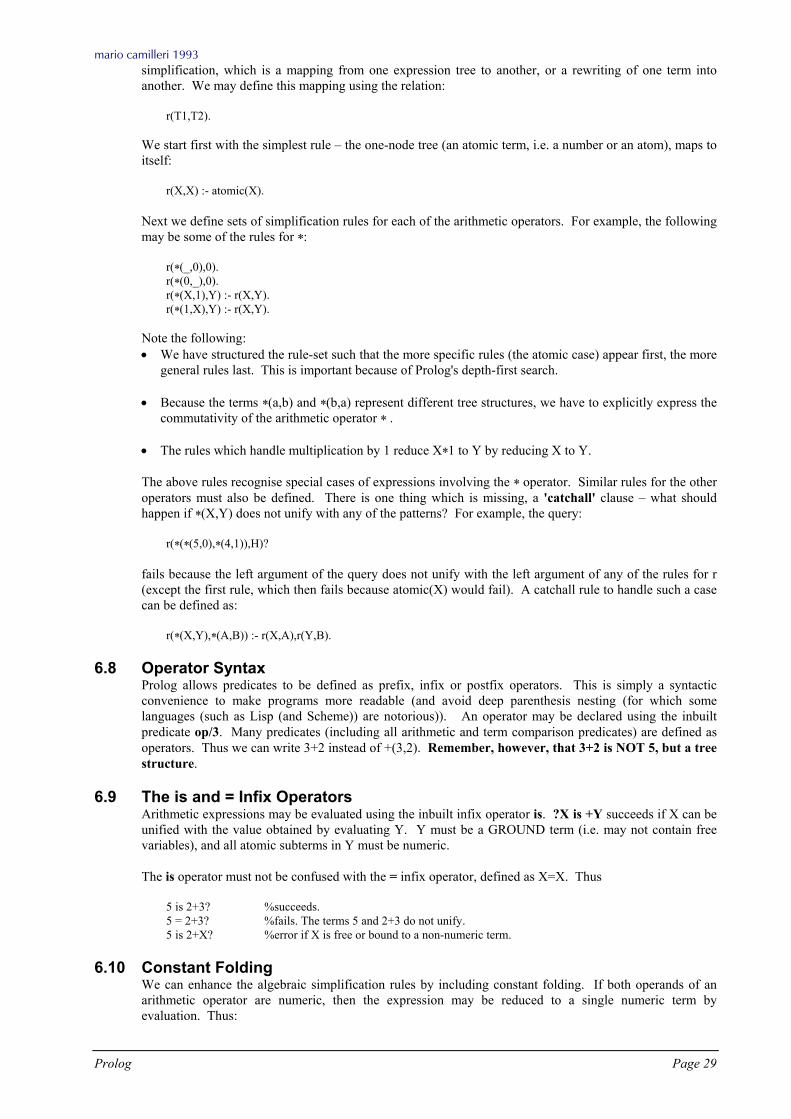
Prolog Page 30
% Boundary condition for r r(X,X) :- atomic(X). % Rules for simplifying multiplication. r(X∗0,0). r(0∗X,0). r(1∗X,Y) :- r(X,Y). r(X∗1,Y) :- r(X,Y). r(X∗Y,Z) :- numeric(X), numeric(Y), Z is X∗Y. %Constant folding. r(X∗Y,A∗B) :- r(X,A), r(Y,B). %Catchall for ∗. % and similar sets of rules for the other operators.
Suppose now we have the query
r((a∗0)∗(b∗1),H)?
This unifies with the head of the catchall clause, instantiating X to a∗0, Y to b∗1 and H to A∗B. The rule then recurses on X, instantiating A to 0. It recurses again on Y, instantiating B to b. So the variable H in the query is instantiated to 0∗b. There are 3 problems with this program: 1. Because of backtracking, an expression will be simplified in many different ways. Because of the way
the rules are structured (special cases first and general case last), the first answer will be the most simplified. Actually, the above rules are mutually exclusive, and so cuts are needed to reflect this.
2. For the commutative operators ∗ and +, the rules described above may have different effects on
expressions that are written differently but are algebraically equivalent. For example, the folding rule will correctly simplify 2∗3∗a to 6∗a, but a∗2∗3 will be mapped to itself. This is because:
*
2 3
*
a
2*3*a =
*
a 2
*
3
a*2*3 =
In the leftmost tree, the bottomost multiplication can be folded to 6. In the rightmost, no subtree can be folded. Solving this problem for the general case is possible, but will require much more sophisticated rules.
3. The rules perform only a single simplification of the expression tree. The resulting expression may be further simplifiable. To perform all possible simplifications (within the constraints of the rules we have), a driver predicate is needed which recursively simplifies an expression until no further simplifications are possible. Writing such a driver is simple. The bottom line is r(X,X) � X simplifies to itself. The driver predicate can be defined as:
simp(Exp,Reduced) :- r(Exp,R), R \= Exp, !, simp(R,Reduced). simp(Exp,Exp).
The predicate simp also solves problem 1 above, because once Exp has been simplified by a rule r, the ! will prevent further backtracking.
6.11 Exercises 1. Write a predicate or(+X,+Y) which succeeds if either X or Y succeed. If X succeeds, then Y should not
be called.
2. Write a predicate same(+X,+Y), where X and Y are arithmetic expressions. The predicate should
succeed if the two expressions are equivalent, taking the commutativity of + and ∗ into consideration. For example,

mario camilleri 1993
Prolog Page 31
same(a+b∗c,c∗b+a)?
should succeed. Make sure your predicate does not get caught in an infinite loop!
3. Complete the simplification program by adding simplification rules for the other arithmetic operators.
Try to use the same/2 predicate to write more efficient rules, e.g.
r(X-Y,0) :- same(X,Y).

mario camilleri 1993
Lists in Prolog Page 32
7 Lists in Prolog
In the previous chapter we introduced compound terms to represent arbitrary tree structures in Prolog. In this chapter we take a closer look at one form of tree structure which is of special interest � the list.
7.1 Representing Lists using Compound Terms Since Prolog's terms can represent arbitrary tree structures, they can also represent lists, since a list is just a special form of tree sometimes called a vine. All we need is a binary relation (arity 2) to represent an internal node of the vine, and a constant atom to represent the empty list. We will represent the list
a,b,c,d as
cons(a, cons(b, cons(c, cons(d,nil)))) Our list-constructor cons/2 takes an element as its first argument, and a list continuation as its second argument, thus:
cons(Head,Tail)
7.2 Operations on Lists Like any other data structure, a list is defined NOT by its representation, but by the operations we define on it. Using the representation above, we can easily define a predicate which counts the element in the list:
len(nil,0). len(cons(_,Tail),L) :- len(Tail,TL), L is TL+1.
And a predicate which checks for membership: member(Item, cons(Item,_)). member(Item, cons(_,Tail)) :- member(Item, Tail).
7.3 Adding Syntactic Sugar The notation we have been using for lists is cumbersome, and ∴ Prolog provides a more convenient notation, allowing us to represent: • the empty list as the atom [ ], and
• a nonempty list as for example [a,b,c,d].
In this notation, the list constructor cons(Head,Tail) is written as [Head | Tail] (or equivalently as [Head ..Tail]). It is important to keep in mind that all we have changed is the syntax. Thus, in [H | T], H is an element of the list, but T is a list (the original list minus the first element). Also, [a | [b,c]] is equivalent to [a,b,c].
a
b
c
d nil
A vine representing the lista,b,c,d. Note how at each nodeof the vine, the left subtree is aleaf, while the right subtree is alist (nil being the empty list).

mario camilleri 1993
Lists in Prolog Page 33
7.4 Unification on Lists Since lists are just trees, unification works on lists just as it does on trees. However, the syntactic differences may not make this immediately obvious. The following table gives some examples of the result of unifying (or attempting to unify) lists: Term 1 Term 2 Comments a [a] unification not possible [a] [H|T] H=a, T=[] [a,b,c] [A|B] A=a, B=[b,c] [[a],b,c] [H|T] H=[a], T=[b,c] [a,b,c] [E,F | G] E=a, F=b, G=[c] [] [H|T] unification not possible
7.5 Elementary List Predicates List predicates typically work by analysing the first element of the list, and then possibly recursing on the tail. The following definitions should give some feel for how to handle lists:
% last(Element,List) % last(c,[a,b,c])? will succeed % last(X,[a,b,c])? will succeed with X=c last(X,[X]). last(X,[_|T]) :- last(X,T). % len(List,Num) % len([a,b,c],3) succeeds % len([a,b,c],N) succeeds with N=3 len([],0). len([_|T],N) :- len(T,NT), N is NT+1 % member(Element,List) % member(b,[a,b,c])? will succeed % member(X,[a,b,c])? will succeed with X=a, then X=b, then X=c member(X,[X|_]). member(X,[_|T]) :- member(X,T).
The member/2 predicate can be used as a generator, which on backtracking will bind Element to successive elements of the list. For example, here's a predicate which prints the elements of a list as a column. It makes use of fail/0 to force member/2 to generate all elements E of L:
plist(L) :- member(E,L), print(E), fail.
The following predicate succeeds if E1 appears immediately before E2 in a list L: % adj(E1,E2,L) % adj((b,c,[a,b,c]) succeeds % adj(b,X,[a,b,c]) succeeds with X=c % adj(X,b,[a,b,c]) succeeds with X=a % adj(b,X,[a,b,c,b,d]) succeeds with X=c, then with X=d % adj(X,Y,[a,b,c]) succeeds with X=a, Y=b, then with X=b, Y=c adj(E1,E2,[E1,E2|_]). adj(E1,E2,[_|T]) :- adj(E1,E2,T).
7.6 The nth Element of a List Consider the following predicate for finding the nth element of a list:
nth(1,[H|_],H). nth(N,[_|T],H) :- N2 is N-1, nth(N2,T,H).
Basically this says that the first element of a list is its head, and that the Nth element of a list is the (N-1)th element of its tail. However, the definition of nth/3 has a flaw � it will not work if N is free, because is/2 requires its right-hand term to be ground. Thus, all the following will produce an arithmetic error:
nth(N,[a,b,c,d,e],d)? nth(N,[a,b,a,c,d,a],a)? nth(N,[a,b,c,d,e],E)?
mario camilleri 1993
Lists in Prolog Page 34
A better definition of nth/3 is as follows:
nth(1,[H|_],H). nth(N,[_|T],H) :- nth(N2,T,H), N is N2+1.
This works because, in the second clause, the is/2 predicate can only be reached if N2 has already been instantiated. This version is, however, less efficient.
7.7 Appending Lists Append/3 defines a relation between three lists L1, L2 and L1L2, such that, for example, append([a,b],[c,d],[a,b,c,d]).
% append(L1,L2,L1L2). append([],L,L). append([H|T],L,[H|T2]) :- append(T,L,T2).
It is important to keep in mind that append/3 is a relation, not a function. Thus it can be used in various ways, and not simply to add L1 to the front of L2. For example: append(X,[d,e],[a,b,c,d,e])? succeeds with X=[a,b,c] append(X,Y,[a,b,c])? succeeds four times, with X = [] Y = [a, b, c] X = [a] Y = [b, c] X = [a, b] Y = [c] X = [a, b, c] Y = [] This multi-way capability of the append/3 predicate makes it possible to define last/2, adj/2 and member/2 in terms of append/3 as follows:
last(Element,List) :- append(_,[Element],List). member(Element,List) :- append(_,[Element|_],List). adj(E1,E2,List) :- append(_,[E1,E2|_],List).
7.8 Reversing a List The simplest way to relate a list L with its mirror image R is as follows:
% rev(List,Reverse) rev([],[]). rev([H|T],R) :- rev(T,RT), append(RT,[H],R).
We can use rev/2 to test whether a list reads the same both ways (a palindrome), e.g. [r,a,d,a,r]: palindrome(L) :- rev(L,L).
7.9 Deleting and Replacing Elements from a List So far, all list predicates have followed a simple 2-clause structure � a boundary clause, and a recursive clause. The following predicates need 2, mutually exclusive, recursive clauses � one for when an element of interest is at the head of the list, one for when the element of interest is NOT the head of the list. The ! predicate is used to express this mutual exclusion.
% del(Element,List1,List2). % Constructs List2 from elements of List1 which are % not equal to Element. del(_,[],[]). del(E,[E|T],T2) :- !,del(Element,T,T2). del(E,[H|T],[H|T2]) :- del (E,T,T2).
Replacing an element E1 in List1 by E2 in List2 works similarly: % rep(E1,L1,E2,L2). % rep(b,[a,b,c],x,L)? succeeds with L=[a,x,c] rep(_,[],_,[]). rep(E1,[E1|T1],E2,[E2|T2]) :- !,rep(E1,T1,E2,T2).
mario camilleri 1993
Lists in Prolog Page 35
rep(E1,[H|T1],E2,[H|T2]) :- rep(E1,T1,E2,T2).
The following predicate filter/2 maps a list L1 to a list L2 if L2 consists of the same elements of L1, in the same order, with all multiple occurences of an element except the last removed. Thus filter([a,b,c,b,a,c],[b,a,c]).
% filter(List,FilteredList) filter([],[]). filter([H|T],L) :- member(H,T),!,filter(T,L). filter([H|T],[H|T2]) :- filter(T,T2).
Note how the second clause uses member/2 and ! to distinguish the case where the element under consideration occurs elsewhere down the list, from the case where the element is the only remaining occurence (handled by clause 3).
7.10 List Application Sometimes we want to apply the same predicate to each element of a list � for example
∀ I ∈ List print(I). We can define a predicate which takes some predicate P/1 and a list, and applies the predicate to each element:
% app(+Predicate,List). app(_,[]). app(P,[H|T]) :- P(H)6,app(P,T).
Thus, the goal app(print,[a,b,c])? will call print/1 for each element of [a,b,c]. Note that app(P,L)? will succeed iff P(i) succeeds for all i in L. Thus it can also be used to check whether all elements in a list satisfy some condition. For example:
app(numeric,L)?
succeeds iff all elements in list L are numeric.
7.11 List Mapping Sometimes we want to construct a list L2 from a list L1 by consistently mapping each element of L1 into a corresponding element of L2. A binary relation performs the mapping. Recall, for example, the married(Husband,Wife) predicate from the family knowledgebase. We may wish to map a list of husbands into a corresponding list of wives. We can do this as follows:
maphusbands([],[]). maphusbands([H|Th],[W|Tw]) :- married(H,W), maphusbands(Th,Tw).
Thus maphusbands([anthony,bill,claude],W)? succeeds with W = [ann, bella, carol] and maphusbands(H,[ann,carol,daphne])? succeeds with H = [anthony, claude, dominic] Alternatively, we can write a general predicate map/3 which takes a predicate P/2 and two lists L1 and L2, and maps L1 into L2 by applying P(E1,E2) to each corresponding pair of elements in the two lists:
map(_,[],[]). map(P,[E1|T1],[E2|T2]) :- P(E1,E2), map(P,T1,T2).
We could then have map(married,[anthony,bill,claude],W)? instead of using maphusband/2. the map/3 predicate is also very useful for manipulating lists of numbers, for example:
% succ(N1,N2) if N2 is N1+1 succ(A,B) :- B is A+1. map(succ,[2,5,-1,6],L)? succeeds with L=[3,6,0,7]
Note that, because is/2 requires the right-hand side argument to be ground (i.e. contains no free variables), succ/2 will only work if A is instantiated (obviously to a number). This prevents succ/2 from doubling as
6 Not all Prolog implementations will allow a call of the form P(H). These tend to be the same implementations which insist on the
use of the predicate call/1 (see previous chapter). In this case, P(H) will need to be rewritten as: X =.. [P,H], call(X) The UNIV operator =.. relates the term f(a,b,c) to the list [f,a,b,c].
mario camilleri 1993
Lists in Prolog Page 36
pred/2. This problem is similar to the one for nth/3, and is common when using arithmetic in Prolog7. In this case, we can overcome this limitation of succ/2 by using metaprogramming � having mutually exclusive clauses for different states of the arguments:
succ(A,B) :- nonvar(A), !, B is A+1. succ(A,B) :- nonvar(B), A is B-1.
Now, succ(2,N)? succeeds by clause 1, binding N to 3, while succ(N,8)? succeeds by clause 2, binding N to 7.
7.12 Exercises 1. Using filtered lists to represent sets, implement set predicates:
union(Set1,Set2,Union). Union = Set1 ∪ Set2 intersect(Set1,Set2,Intersect). Intersect = Set1 ⊨ Set2 difference(Set1,Set2,Diff). Diff = {e | (e∈Set1) and (e∉Set2)} subset(Sub,Set). Sub ⊆Set equal(Set1,Set2) (Set1 ⊆ Set2) and (Set2 ⊆ Set1) disjoint(Set1,Set2). (Set1 ⊨ Set2) = ∅
2. Write a predicate listp(L) which succeeds iff L is a list (just as numeric(X) succeeds iff X is a number).
3. Without using the not/1 predicate, write a predicate notmember(X,L) which succeeds iff X is NOT a member of L.
4. Write a 2-clause predicate
insert(Element, Position, List1, List2) Such that List2 is identical to List1 except that it has Element inserted in position Position. The only
restriction on the parameters of insert/4 is that at least ONE parameter must be bound. Thus insert(a,3,[1,2,3,4],[1,2,a,3,4])? ** yes insert(a,3,[1,2,3,4],[1,2,a,3])? ** no insert(a,3,[1,2,3,4],[1,2,3,a,4])? ** no insert(A,3,[1,2,3,4],[1,2,c,3,4])? A = c insert(A,B,[1,2,3,4],[1,2,c,3,4])? A = c, B = 3 insert(a,2,[1,2,3,4],L)? L = [1, a, 2, 3, 4] insert(a,5,L,[1,2,3,a,4])? ** no
5. Write a program to solve the 8-Queens problem � to find all ways of arranging 8 queens on a standard
chess board such that no queen is in a position to take any of the others (queens move any number of squares diagonally, horizontally or vertically). Your program should find all 92 solutions, and display each using character-based graphics.
7 Originally, Prolog was developed in the early 1970s for use in natural-language processing, and thus hardly offered any support
for arithmetic. This deficiency has been set right in PrologII and PrologIII, as we'll see later in the chapter on constraint logic programming.
mario camilleri 1993
The Unification Mechanism Page 37
8 The Unification Mechanism
In this chapter we consider the unification mechanism in more detail, and show how unification is in fact a mechanism for solving systems of equations over the domain of tree structures (in the case of Prolog, the domain of finite tree structures). We finally take a brief look at recent developments in logic programming which replace unification by a more general constraint mechanism which is capable of solving systems of equations over other domains besides that of tree structures.
8.1 Instances of Universally Quantified Clauses Consider the Prolog clause:
a(f(X,Y)) :- b(X),c(Y). which represents the following logic formula:
∀X,Y (b(X) ∧ c(Y)) ⇒ a(f(X,Y)) Basically this is a statement about elements of a domain of tree structures: elements of the domain called a are ordered trees having a root f and two subtrees X and Y, with X being in domain b and Y in the domain c. Assuming that the knowledgebase contains clauses for predicates b/1 and c/1 (thus defining these particular domains), a query such as
a(f(2,3))? requests a search of the domain a for the element f(2,3). The search need not be exhaustive � i.e. there is no need to generate all elements of the (possibly infinite) domain a and then test for the presence or otherwise of a(f(2,3)) in that set. Instead we proceed as follows:
∀X,Y (b(X) ∧ c(Y)) ⇒ a(f(X,Y)) a(f(2,3)) is an INSTANCE of a(f(X,Y)), with X←2, Y←3 ∴ (b(2) ∧ c(3)) ⇒ a(f(2,3))
The main thing is to recognize that a(f(2,3)) is an INSTANCE of the more general a(f(X,Y)), obtained by an appropriate substitution of variables, which is allowed because the variables are universally quantified. Example: The following clauses define the domain of well-formed propositional formulae (limited to the 3 truth functions and/2, or/2 and not/1 expressed in function notation):
1. wff(X) :- atom(X). ;an atomic formula 2. wff(not(X)) :- wff(X). 3. wff(and(X,Y)) :- wff(X), wff(Y). 4. wff(or(X,Y)) :- wff(X), wff(Y).

mario camilleri 1993
The Unification Mechanism Page 38
The proof of the query wff(and(a, or(b,c)))? proceeds as follows: by 3: wff(and(a, or(b,c))) :- wff(a), wff(or(b,c)). by 1: wff(a) :- atomic(a). %proven by 4: wff(or(b,c)) :- wff(b), wff(c). by 1: wff(b) :- atomic(b). %proven by 1: wff(c) :- atomic(c). %proven
8.2 Substitutions A substitution θ is a set of replacements of the form X←α, where X is a variable and α is a term (variable, constant or structure)8. The application of a substitution θ to a formula F, written Fθ (read F under θ), involves simultaneosly applying every replacement in θ throughout F. By this we mean that every replacement in θ is independent of every other replacement. Example Let
F = a(f(X,Y)) :- b(X),c(Y). θ = {X=g, Y=f(1,2)}
then Fθ = a(f(g,f(1,2))) :- b(g), c(f(1,2)). Fθ is stb an INSTANCE of F. Thus, a(f(2,3)) is an instance of a(f(X,Y)). We place 2 restrictions on substitutions: 1. A substitution must define a function. Thus there can only be a single replacement for a variable (i.e.
no two replacements can have the same left-hand side). {X=a, X=b} is not a legal substitution.
2. A substitution must be idempotent so that, for any formula F and substitution θ, (Fθ)θ = Fθ. This requires that a variable cannot appear both on the left and on the right of replacements. Thus, both {X←f(X)} and {X←a, Y←X} are not legal substitutions.
8.3 The Idempotence Constraint The idempotence constraint is necessary because our domain of interest is finite trees, which we would like to be closed under substitution application. If F is a finite tree, we want Fθ to be a finite tree. If θ is not idempotent, Fθ may be a cyclic graph (infinite tree). Example If θ = {X←f(X)}, a substitution which is not idempotent, and F = a(X,b) then Fθ = the cyclic graph (infinite tree) a(f(f(f(......))),b)
8.4 Composition of Substitutions The composition of two substitutions ρ = θ⋅σ involves applying σ to the rhs of each replacement in θ. Example Let θ = {U←W, X←Y, Z←a} σ = {T←e, W←V, Y←b, Z←d} Then ρ = θ⋅σ = {U←V, X←b, Z←a, T←e} Let f = a(U,s,X,Z) Then fθσ = fρ = a(V,s,b,a)
8 Other notations besides X←α used to denote a replacement are X=α and α/X.
mario camilleri 1993
The Unification Mechanism Page 39
Note that the composition of 2 substitutions is NOT necessarily a substitution, because it may violate the idempotence constraint. Thus substitutions (as we have defined them) are not closed under composition. For example, if θ = {X←U} and σ = {U←f(X)} Then ρ = θ⋅σ = {X←f(X)} is not idempotent and therefore is not a legal substitution. For substitutions to be closed under composition, we must remove the idempotence constraint � but then finite trees are not closed under application of substitutions. We therefore define composition of substitutions ONLY for substitutions θ and σ s.t. θ⋅σ is idempotent. If not, then θ⋅σ is not defined. NOTE that composition of substitutions (when defined) • is associative
• is not generally commutative
• has the empty substitution ε = {} as identity
8.5 Unifiers Let S = {F1, F2, ..., Fn} be a set of formulae, and θ a substitution. Then θ is stb a UNIFIER of the set S if F1θ = F2θ = ... = Fnθ. Example Let F1 = p(X,b,Z) F2 = p(Y,W,a) F3 = p(Y,b,Z) Then θ = {W←b, X←c, Y←c, Z←a} is a unifier of the set {F1,F2,F3}, because F1θ = F2θ = F3θ = p(c,b,a). A unifier for a set of formulae may not exist. If a unifier exists, then we say that the formulae are UNIFIABLE. A unifier for a set of formulae may not be unique. From the example above, the substitution σ = {W←b, X←i, Y←i, Z←a} is also a unifier of the set. If a formula set S is unifiable, then there exists a unifier µ, called a MOST GENERAL UNIFIER (MGU), with the property that, for any unifier θ of S, θ = µ⋅θ. 9 In other words, every unifier of S is an instance of the MGU µ of S. A MGU need not be unique. For the example above, µ = {W←b, X←Y, Z←a} is a MGU (and so is {W←b, Y←X, Z←a}).
8.6 Unification Algorithms A unification algorithm computes an MGU for a (finite) set of formulae if the set is unifiable, otherwise detecting that the set is not unifiable. We will only consider unification of pairs of terms (trees). NOTE that it is assumed that the two trees have no variables in common (this may require renaming to avoid name clashes). In unifying two terms T1 and T2, we traverse the two term trees in parallel in pre-order, noting disgareement between corresponding node pairs. A disagreement between nodes N1 and N2 of trees T1 and T2 respectively is REPARABLE if at least one of N1,N2 (say N1) is a free variable. The substitution {N1←N2t} (where N2t is the subtree of T2 rooted at N2) will repair this disagreement iff N1 does NOT OCCUR in N2t (otherwise the resulting substitution is not idempotent). This subsitution must be applied to the two trees before traversal continues, since all occurences of N1 must be replaced by N2. The MGU of T1 and T2 is the composition of all the substitutions required to repair node disagreements.
9 Some texts do not impose the idempotence constraint on substitutions, and define a MGU as a unifier µ st for any unifier θ there
exists a substitution σ for which θ = µ⋅σ. In our case, since all substitutions are idempotent, µ = µ⋅ µ, and ∴ if θ = µ⋅σ, then θ = µ⋅µ⋅σ, so θ = µ⋅θ (since composition of substitutions is associative).

mario camilleri 1993
The Unification Mechanism Page 40
If a disgareement is not reparable (as when N1 and N2 are different atoms, or the OCCUR CHECK fails), then the terms are not unifiable. The following algorithm computes the MGU of two terms, returning FALSE if the terms are not unifiable10. The algorithm is passed the two terms and the empty substitution {} as parameters, and returns the MGU of the terms if they are unifiable.
Function Unify(T1,T2 : term trees; VAR µ: substitution) : boolean; 1. Let N1 := root node of T1 µ 2. Let N2 := root node of T2 µ 3. OK := TRUE; 4. If either of N1,N2 is the anonymous variable then exit with OK 5. If N1,N2 are the same variable then exit with OK 6. If N1=N2 then 7. Begin 8. i := 1 9. While OK and (i < arity(N1)) do 10. OK := Unify(subtree i of T1, subtree i of T2, µ) 11. end 12. else if (var(N1)) and (Not OCCURS(N1,T2µ)) then µ := µ ⋅ {N1←T2µ} 13. else if (var(N2)) and (Not OCCURS(N2,T1µ)) then µ := µ ⋅ {N2←T1µ} 14. else OK := FALSE 15. Unify := OK
Notes: 1,2 We take nodes from the term instances (i.e. we take the current substitution into account). So, if
T1= X and µ={X←a}, T1µ=a and N1 would be a. The same happens elsewhere in the algorithm, where we always need to consider T1µ and T2µ. Of course, in an actual implementation things would be done in a more efficient way.
6 N1=N2 if symbol(N1)=symbol(N2) and arity(N1)=arity(N2) � the two nodes are considered to be equal iff they have the same node label, and the same out-degree.
10 Here we recurse for each pair of subtrees. 12,13 The occurs check is performed before composition to ensure that µ remains idempotent.
8.7 Prolog and Cyclic Structures Most Prolog implementations do not perform the OCCURS CHECK during unification, because this check tends to be computationally expensive. Moreover, in the majority of (well-written) Prolog programs the check is not necessary anyway. The result is that it is possible to unwittingly generate cyclic structures (infinite trees) which the implementation cannot handle. The following query will typically cause a runtime error in implementations which omit the occurs check, but will fail in those which do: X=f(X)? Similarly, unifying the following 2 terms will generate a cyclic structure: f(X,X). f(Y,g(Y)). because this is equivalent to Y=g(Y).
8.8 Constraint Logic Programming Prolog unification can be viewed as a mechanism for solving systems of equations over the domain of ordered finite trees. Constraint Logic Programming generalizes this mechanism to solving systems of equations (and inequations) over other domains11. The solution is required to simultaneously satisfy a number of constraints. Consider the following:
1 + A = 5
10 For a parallel unification algorithm see Robinson,J.A. (1992) 'Logic and Logic Programming' in CACM March '92 pp.48-51. 11 See Cohen,J. Constraint Logic Programming Languages, and Colmerauer,A. An Introduction to Prolog III, both in CACM July
1990.

mario camilleri 1993
The Unification Mechanism Page 41
In Prolog, 5 and 1+A are treated as trees, and X=Y iff X and Y are unifiable. Since there exists no unifier for 5 and 1+A, this fails. However, we can also think of
1 + A = 5
as a constraint on the variable A � both on its type (numeric) and its value (4). Similarly, A=B∗2 constrains A and B to only certain values. There are two (unsatisfactory) ways of expressing this in Prolog. The first is to explicitly define Peano's axioms (in terms of constant 0 and the successor function � thus representing 1 as the structure s(0), 2 as s(s(0)), etc � essentially a unary system). We let the relation:
add(X,Y,Z)
represent X+Y= Z. We can then define addition as
add(0,Y,Y). add(s(X),Y,s(Z)) :- add(X,Y,Z).
The equation 1+A=5 can then be expressed as the query
add(s(0),A,s(s(s(s(s(0))))))?
Unfortunately, using this method is only feasible for small integers � it is very much like programming using Turing machines! The second way is to bypass the unification mechanism altogether, and resort to metaprogramming as follows:
add(X,Y,Z) :- nonvar(X), nonvar(Y), !, Z is X+Y. add(X,Y,Z) :- var(X), nonvar(Y), nonvar(Z), X is Z-Y. add(X,Y,Z) :- var(Y), nonvar(X), nonvar(Z), Y is Z-X.
This method is also unsatisfactory, because the equation X+Y=Z is only solvable if at most one of X,Y,Z is unknown.
8.9 CLP Languages CLP languages such as CLP(R) and PrologIII provide a more elegant solution to this problem � they replace unification by constraints on elements of various domains, such as equality and inequality of arithmetic expressions. Because these constraint solvers are specialized to particular domains, they can take into account properties specific to the domain, such as associativity, comutativity and reflexivity of operations. Constraint solvers work by postponing the binding of a variable until sufficient constraints have been accumulated to completely bind the variable. If at any point the set of accumulated constraints becomes unsatisfiable, failure results, and if possible backtracking occurs.
8.10 Examples of CLP Programs The following are some examples of CLP programs written in a PrologIII-like language. The first example defines the predicate even/1 on the domain of integers:
even(2∗M) :- integer(M). even(10)? ;succeeds
Note that the query even(X)?, where X is a variable, will succeed, but will leave X still only partially bound to the pair of constraints (X=2∗M, integer(M)). The next example defines the fibonacci numbers Fn = Fn-1 + Fn-2, with F0=1, F1=1.
fib(0,1). fib(1,1). fib(N,R1+R2) :- N ≥ 2, fib(N-1,R1), fib(N-2,R2). fib(10,F)? ;succeeds with F=89 fib(N,89)? ;succeeds with N=10

mario camilleri 1993
The Unification Mechanism Page 42
Note the constraint N≥2 in the 3rd clause above. This constraint could not have been expressed in Prolog unless N is guaranteed to be instantiated to a number � which would have ruled out the second query. The following CLP clauses define the relation between a list of digits and the number it represents. The expression X�Y, defined over lists, represents the concatenation of the two lists X and Y. Thus, if L is a list and A,B are free variables, L = A�[B] would bind B to the LAST element of L, while L = [A]�B would bind A to the HEAD of L and B to the tail.
value([],0). value(X�[N], 10∗M+N) :- value(X,M). value([1,2,3,4],X)? ;succeeds with X=1234 value(X,1234)? ;succeeds with X=[1,2,3,4]
The following constrains L to be a list of even length, made up of the two halves H1 and H2, where |H1| represents the length of list H1 (similarly |H2|):
L = H1�H2, |H1| = |H2|?
while the following creates a list L of 100 a's:
[a]�L = L�[a], |L|=100?

mario camilleri 1993
The Unification Mechanism Page 43
PROJECTS
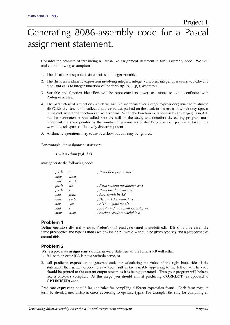
mario camilleri 1993
Generating 8086-assembly code for a Pascal assignment statement. Page 44
Project 1 Generating 8086-assembly code for a Pascal assignment statement.
Consider the problem of translating a Pascal-like assignment statement to 8086 assembly code. We will make the following assumptions: 1. The lhs of the assignment statement is an integer variable.
2. The rhs is an arithmetic expression involving integers, integer variables, integer operations +,-,∗,div and mod, and calls to integer functions of the form f(p1,p2,...,pn), where n≥1.
3. Variable and function identifiers will be represented as lower-case atoms to avoid confusion with Prolog variables.
4. The parameters of a function (which we assume are themselves integer expressions) must be evaluated BEFORE the function is called, and their values pushed on the stack in the order in which they appear in the call, where the function can access them. When the function exits, its result (an integer) is in AX, but the parameters it was called with are still on the stack, and therefore the calling program must increment the stack pointer by the number of parameters pushed∗2 (since each parameter takes up a word of stack space), effectively discarding them.
5. Arithmetic operations may cause overflow, but this may be ignored.
For example, the assignment statement a ≔ b ∗ - func(x,d+3,t) may generate the following code: push x ; Push first parameter mov ax,d add ax,3 push ax ; Push second parameter d+3 push t ; Push third parameter call func ; func result in AX add sp,6 ; Discard 3 parameters neg ax ; AX <- - func result mul b ; AX <- (- func result (in AX)) ∗ b mov a,ax ; Assign result to variable a
Problem 1 Define operators div and ≔ using Prolog's op/3 predicate (mod is predefined). Div should be given the same precedence and type as mod (see on-line help), while ≔ should be given type xfy and a precedence of around 600.
Problem 2 Write a predicate assign(Stmt) which, given a statement of the form A≔B will either 1. fail with an error if A is not a variable name, or
2. call predicate expression to generate code for calculating the value of the right hand side of the statement, then generate code to save the result in the variable appearing to the left of ≔. The code should be printed to the current output stream as it is being generated. Thus your program will behave like a one-pass compiler. At this stage you should aim at producing CORRECT (as opposed to OPTIMISED) code.
Predicate expression should include rules for compiling different expression forms. Each form may, in turn, be divided into different cases according to operand types. For example, the rule for compiling an

mario camilleri 1993
Generating 8086-assembly code for a Pascal assignment statement. Page 45
expression of the form A+B might generate different code depending on whether either argument is atomic or not.
Problem 3 Consider (and attempt to implement) ways in which the code generated may be optimised. You may try to simplify the right hand side of the assignment before compiling it, reduce unnecessary movement of operands to/from memory and between registers, and recognise common subexpressions (which therefore need only be calculated once). One optimisation technique will be enough.
Problem 4 Make your program automatically annotate the code it generates.

mario camilleri 1993
Rewriting propositional formulae into simplified, nand-2 form. Page 46
Project 2 Rewriting propositional formulae into simplified, nand-2 form.
Consider the problem of representing propositional logic formulae involving connectives not, ∧ (and), ∨ (or), ⇒ and ⇔, the constants t (true) and f (false), and propositional symbols (not confusable with t and f), as in:
not(a) /\ t \/ b
a. Prolog will not accept the above expression, since /\, \/, => and <=> are nor inbuilt operators. Declare these 4 operators using the Prolog predicate op/3 (see C&M 1st edn. pp108ff, as well as Prolog86's on-line help), making sure you give them the correct precedence and associativity.
b. Write a predicate leq(A,B), which succeeds if A and B are logically equivalent. Thus, the following
should all succeed:
leq(a /\ b, b /\ a)? leq((a \/ b) <=> c, c <=> (b \/ a))?
c. Write a predicate psimp(+A,-B) which, given a propositional expression A, rewrites it in a (possibly) simplified form as B. For example:
psimp((x /\ y) \/ not(y /\ x),B)? B = t
Try to make psimp/2 as complete as possible. You may also wish to have psimp/2 rewrite expressions involving =>, <=> and \/ to expressions involving only not and /\ (this will simplify step e later on).
d. psimp/2 performs a single reduction step. Write a predicate psimplify(+A,-B), which performs all
possible reductions on an input expression A, rewriting it to B. e. In the manufacture of logic circuits, it is often advantageous to employ only a single type of gate � for
example a 2-input nand gate. Write a predicate nsimp(+A,-B) which takes an arbitrary propositional expression A, and rewrites it to a logically equivalent expression B using only 2-input nands. You may define nand as an infix Prolog operator, or use a structured term nand(A,B) to represent A nand B.
f. Write a main predicate nsimplify(+A,-B) which rewrites an arbitrary propositional expression A to a
(completely) simplified, logically equivalent, 2-input-nand-expression B. nsimplify/2 will be your main program. Test it on the following:
nsimplify ( not(a => b), B)? B = nand(nand(a, nand(b, b)), nand(a, nand(b, b)))
nsimplify (a \/ a, B)? B = a
nsimplify (a /\ not(a) => b, B)? B = t
nsimplify (a /\ b \/ (c /\ d), B)? B = nand(nand(a, b), nand(c, d))
nsimplify (not(a) \/ not(b), B)? B = nand(a, b)
mario camilleri 1993
Symbolic manipulation of algebraic expressions. Page 47
Project 3 Symbolic manipulation of algebraic expressions.
Problem 1 Write a predicate
fx(Exp,Var)
where: 1. Exp is an arbitrary algebraic expression involving integers, symbolic variables (represented as atoms),
operators (+,-,etc) and arbitrary function symbols (sin(u), f(a,b,c),etc).
2. Var is a symbolic variable (represented as an atom).
The predicate fx succeeds iff Exp is a function of Var, which may be defined as follows: 1. If Exp is atomic, then it is a function of Var iff Exp=Var
2. If Exp is a compound expression then Exp is a function of Var iff any of its subexpressions or parameters is itself a function of Var.
The following calls should all succeed:
fx (h,h) fx (x+a*3,x) fx (gcd(d,succ(n)),n)
Since the predicate fx should work for arbitrary function symbols (not just operators), you should use the Prolog inbuilt predicate =.. (called UNIV) to examine the operands of Exp (see C&M 1st edn. p123).
Problem 2 Implement symbolic differentiation as a set of Prolog rules of the form:
diff (Exp,Wrt,Deriv)
where Exp is the input algebraic expression to be differentiated, Wrt is an atom representing a variable, and Deriv is d(Exp)/d(Wrt). Attempt to make your rule-base as comprehensive as possible. You may wish to use the predicate fx to trigger different rules according to the form of the input expression (for example, if Exp is not a function of Wrt, then Deriv can be calculated immediately).
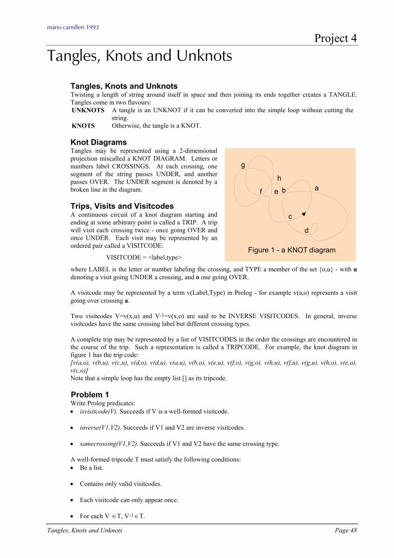
mario camilleri 1993
Tangles, Knots and Unknots Page 48
Project 4 Tangles, Knots and Unknots
Tangles, Knots and Unknots Twisting a length of string around itself in space and then joining its ends together creates a TANGLE. Tangles come in two flavours: UNKNOTS A tangle is an UNKNOT if it can be converted into the simple loop without cutting the
string. KNOTS Otherwise, the tangle is a KNOT.
Knot Diagrams Tangles may be represented using a 2-dimensional projection miscalled a KNOT DIAGRAM. Letters or numbers label CROSSINGS. At each crossing, one segment of the string passes UNDER, and another passes OVER. The UNDER segment is denoted by a broken line in the diagram.
Trips, Visits and Visitcodes A continuous circuit of a knot diagram starting and ending at some arbitrary point is called a TRIP. A trip will visit each crossing twice - once going OVER and once UNDER. Each visit may be represented by an ordered pair called a VISITCODE:
VISITCODE = <label,type>
where LABEL is the letter or number labeling the crossing, and TYPE a member of the set {o,u} - with u denoting a visit going UNDER a crossing, and o one going OVER. A visitcode may be represented by a term v(Label,Type) in Prolog - for example v(a,o) represents a visit going over crossing a. Two visitcodes V=v(x,u) and V-1=v(x,o) are said to be INVERSE VISITCODES. In general, inverse visitcodes have the same crossing label but different crossing types. A complete trip may be represented by a list of VISITCODES in the order the crossings are encountered in the course of the trip. Such a representation is called a TRIPCODE. For example, the knot diagram in figure 1 has the trip code: [v(a,o), v(b,u), v(c,u), v(d,o), v(d,u), v(a,u), v(b,o), v(e,u), v(f,o), v(g,o), v(h,u), v(f,u), v(g,u), v(h,o), v(e,o), v(c,o)] Note that a simple loop has the empty list [] as its tripcode.
Problem 1 Write Prolog predicates: • isvisitcode(V). Succeeds if V is a well-formed visitcode.
• inverse(V1,V2). Succeeds if V1 and V2 are inverse visitcodes.
• samecrossing(V1,V2). Succeeds if V1 and V2 have the same crossing type.
A well-formed tripcode T must satisfy the following conditions: • Be a list.
• Contains only valid visitcodes.
• Each visitcode can only appear once.
• For each V ∈T, V-1∈T.
ab
c
d
ef
g
h
Figure 1 - a KNOT diagram
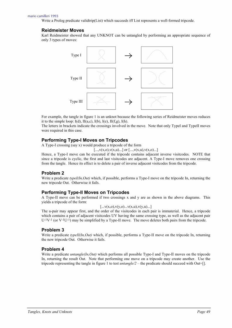
mario camilleri 1993
Tangles, Knots and Unknots Page 49
Write a Prolog predicate validtrip(List) which succeeds iff List represents a well-formed tripcode.
Reidmeister Moves Karl Reidmeister showed that any UNKNOT can be untangled by performing an appropriate sequence of only 3 types of moves:
Type I
→
Type II
→
Type III
→
For example, the tangle in figure 1 is an unknot because the following series of Reidmeister moves reduces it to the simple loop: I(d), II(a,c), I(b), I(e), II(f,g), I(h). The letters in brackets indicate the crossings involved in the move. Note that only TypeI and TypeII moves were required in this case.
Performing Type-I Moves on Tripcodes A Type-I crossing (say x) would produce a tripcode of the form
[...,v(x,o),v(x,u)...] or [...,v(x,u),v(x,o)...] Hence, a Type-I move can be executed if the tripcode contains adjacent inverse visitcodes. NOTE that since a tripcode is cyclic, the first and last visitcodes are adjacent. A Type-I move removes one crossing from the tangle. Hence its effect is to delete a pair of inverse adjacent visitcodes from the tripcode.
Problem 2 Write a predicate typeI(In,Out) which, if possible, performs a Type-I move on the tripcode In, returning the new tripcode Out. Otherwise it fails.
Performing Type-II Moves on Tripcodes A Type-II move can be performed if two crossings x and y are as shown in the above diagrams. This yields a tripcode of the form:
[...v(x,o),v(y,o)...v(x,u),v(y,u)...] The u-pair may appear first, and the order of the visitcodes in each pair is immaterial. Hence, a tripcode which contains a pair of adjacent visitcodes UV having the same crossing type, as well as the adjacent pair U-1V-1 (or V-1U-1) may be simplified by a Type-II move. The move deletes both pairs from the tripcode.
Problem 3 Write a predicate typeII(In,Out) which, if possible, performs a Type-II move on the tripcode In, returning the new tripcode Out. Otherwise it fails.
Problem 4 Write a predicate untangle(In,Out) which performs all possible Type-I and Type-II moves on the tripcode In, returning the result Out. Note that performing one move on a tripcode may create another. Use the tripcode representing the tangle in figure 1 to test untangle/2 � the predicate should succeed with Out=[].


