Journal of Transport Geography 35 (2014) 12–20

Contents lists available at ScienceDirect

Journal of Transport Geography

journal homepage: www.elsevier .com/locate / j t rangeo

Cycling in a changed climate

0966-6923/$ - see front matter � 2014 Elsevier Ltd. All rights reserved.http://dx.doi.org/10.1016/j.jtrangeo.2014.01.001

⇑ Tel.: +44 01133437733.E-mail address: z.wadud@leeds.ac.uk

Zia Wadud ⇑University Research Fellow, Centre for Integrated Energy Research, Institute for Transport Studies and School of Process, Environmental and Materials Engineering, University ofLeeds, Leeds LS2 9JT, United Kingdom

a r t i c l e i n f o

Keywords:Bicycle flowEffects of weatherClimate change impactsClimate change adaptationCount data model

a b s t r a c t

The use of bicycle is substantially affected by the weather patterns, which is expected to change in thefuture as a result of climate change. It is therefore important to understand the resulting potentialchanges in bicycle flows in order to accommodate adaptation planning for cycling. We propose a frame-work to model the changes in bicycle flow in London by developing a negative binomial count-datamodel and by incorporating future projected weather data from downscaled global climate models, a firstsuch approach in this area. High temporal resolution (hourly) of our model allows us to decipher changesnot only on an annual basis, but also on a seasonal and daily basis. We find that there will be a modest0.5% increase in the average annual hourly bicycle flows in London’s network due to a changed climate.The increase is primarily driven by a higher temperature due to a changed climate, although the increaseis tempered due to a higher rainfall. The annual average masks the differences of impacts between sea-sons though – bicycle flows are expected to increase during the summer and winter months (by 1.6%),decrease during the spring (by 2%) and remain nearly unchanged during the autumn. Leisure cycling willbe more affected by a changed climate, with an increase of around 7% during the weekend and holidaycycle flows in the summer months.

� 2014 Elsevier Ltd. All rights reserved.

1. Introduction

Reducing carbon emissions to mitigate climate change andadapting to the potential impacts of climate change have becomea major policy goal in many countries in the world. For example,the UK Government has made a commitment of an 80% reductionin its carbon emissions by 2050. The government is also expectedto publish its first National Adaptation Programme (NAP) to cli-mate change at the end of 2013 (UK Government, 2013). Since per-sonal transport is responsible for a major share of global carbonemissions, reducing carbon emissions from transport is an impor-tant area of action. Within the personal transport sector, cyclinghas received significant attention from the transport and city plan-ners and policymakers due to its zero-carbon credentials. Cyclingalso does not emit any harmful criteria air pollutants, and contrib-utes toward a healthier life. A significant increase in cycling as amode share can also alleviate congestion in road spaces or reducethe burden on a crowded public transport system. Thus cycling as atransport mode has multiple co-benefits.

In the context of climate change, cycling’s role so far has beenprimarily for carbon mitigation. Despite a few studies indicatingthat the energy use and carbon reduction potential for cyclingmay not be very large (e.g. less than 5% in the UK, Pooley et al.,

2010), there are still strong campaigns to encourage cycling in dif-ferent countries because of the multiple benefits (Wittink, 2010;ECF, 2011). The emphasis on cycling for carbon mitigation has re-cently been reiterated in the UK: ‘we see the encouragement of cy-cling and walking, along with improvements to public transport, askey to cutting carbon emissions and enhancing the quality of oururban areas’ (UK Parliament, 2013). The other strategy to combatclimate change – adaptation – has not received much attentionyet, except for some cursory mention, in the context of cycling(e.g. UKCIP, 2011).

The lack of interest in climate adaptation studies for cyclingcould be important. However, even before any adaptation planscan be made, it is necessary to know how cycling can be affectedas a result of a change in the future climate. Cycling is an ‘unshel-tered’ activity and cyclists are directly exposed to the variousweather events such as rain, snowfall, gust or even high and lowtemperatures. Therefore, the effectiveness of the use of bicyclesas a transport mode is often affected by day to day changes in localweather. A change in the climate can alter the future weather pat-tern, which can affect cycling in either a positive or a negative way.It is quite possible that the future weather pattern would discour-age cycling, e.g. if the precipitation increases, as predicted in theUK (Met Office, 2011). This would require adaptation strategiesahead in time either to ensure that cycling continues as a strongtransport mode in the future or to accommodate the modal shiftfrom cycling to other transport modes. On the other hand, it is also

Z. Wadud / Journal of Transport Geography 35 (2014) 12–20 13

conceivable that the future weather pattern will be conducive to alarge uptake of cycling (e.g. due to an increase in temperature incolder regions or vice versa), and this would also require planningto ensure adequate cycling infrastructure in place in time. Unfortu-nately, there is a lack of studies on the potential weather-inducedimpact (either on the direction or on the magnitude) of climatechange on bicycle flows, although two recent studies looked intofuture mode choices (including cycling as a mode) in the Nether-lands and Toronto (Bocker et al., 2013b; Saneinejad et al., 2012).This paper aims to address this gap by developing a frameworkto determine the weather-induced impacts of climate change oncycling and applying that model to London, UK. In doing so, we alsodevelop a bicycle count model for London network, incorporatingweather, as well as other explanatory variables that allows us tounderstand the impact of these additional variables too.

The paper is organized as follows. Section 2 reviews the litera-ture on the impact of weather and climate change on cycling.Section 3 presents the modeling framework and the data used inthe study. Section 4 presents the results with Section 5 drawingconclusions and limitations of the current approach.

2. Review of literature

Central to our research is the impact of the change in weatherpattern induced by climate change. There are a number of studiesdocumenting the impact of weather on travel behaviour, in differ-ent modes of travel. In light of the recent reviews covering alltransport modes by Bocker et al. (2013a) and Koetse and Rietveld(2009), we focus only on those studies specific to cycling. One ofthe first studies to quantitatively investigate the impact of weatheron cycling was by Hanson and Hanson (1977). Since then, the rela-tionship between weather and cycling has received growing atten-tion in at least five different disciplines: transportation, urbanstudies, geography, biometeorology and health. In addition to stud-ies on the quantitative impacts of weather on reported or observedlevel of cycling in these disciplines, there are also studies that lookinto attitudes and barriers to cycling through questionnaire sur-veys (Pooley et al., 2011; Wardman et al., 2007), but this threadof literature is beyond the scope of the present work.

Different types of data with different spatial and temporal res-olution have been used by various researchers to understand theimpact of weather on cycling. These include travel survey data atan aggregate level (census tract, city, county, or state; Parkinet al., 2008; Pucher and Buehler, 2006; Dill and Carr, 2003), indi-vidual travel survey responses (Cervero and Duncan, 2003; Berg-strom and Magnussen, 2003; Winters et al., 2007; Rashad, 2009;Heinen et al., 2011; Flynn et al., 2012; Saneinejad et al., 2012),and bicycle count data at different temporal and spatial resolutions(Phung and Rose, 2007; Ahmed et al., 2010, 2012; Miranda-Morenoand Nosal, 2011; Smith and Kauermann, 2011; Tin et al., 2012;Thomas et al., 2013). Although both cross-sectional and time seriesdata have been employed, the deployment of automatic cyclecounters in many cities in the world has made finer resolution timeseries data readily available in recent years, and a number of recentstudies used bicycle count data at a daily resolution (Phung andRose, 2007; Ahmed et al., 2010, 2012); hourly resolution is notmissing either (Smith and Kauermann, 2011; Miranda-Morenoand Nosal, 2011). Studies on mode choice using individual datafrom travel diary surveys and correlating them with weather datahave also started to appear (Cervero and Duncan, 2003; Saneinejadet al., 2012).

There are a few studies (e.g. Goetzke and Rave, 2011) that inves-tigate the effect of ‘bad’ weather to answer a given research ques-tion, but do not specify the parameters of bad weather. There areothers which investigate the effect of specific weather variables

and these studies are relevant to our review. The weather variablesstudied are, in various functional forms, rain, snow, temperature,wind speed, sunshine hours, fog, thunderstorms, and relativehumidity. Most common among these are rain and temperature,which are present in almost all of the studies. Most studies foundthat cycling decreases in the presence of rain or with an increase inrainfall (Keay, 1992; Emmerson et al., 1998; Nankervis, 1999;Richardson, 2000; Cervero and Duncan, 2003; Dill and Carr,2003; Pucher and Buehler, 2006; Brandenburg et al., 2007; Winterset al., 2007; Parkin et al., 2008; Phung and Rose, 2007; Ahmedet al., 2010, 2012; Heinen et al., 2011; Smith and Kauermann,2011; Miranda-Moreno and Nosal, 2011; Buehler and Pucher,2012; Flynn et al., 2012; Tin et al., 2012; Thomas et al., 2013). Onlya few studies found that rain had no statistically significant effecton cycling, and most of those (e.g. Dill and Carr, 2003; Rashad,2009; Buehler and Pucher, 2012) utilize cross-sectional inter-cityor inter-county data, which could be prone to omitted variable bias.

There is also a consensus on the effect of temperature (exceptBuehler and Pucher, 2012): up to a certain temperature, an in-crease in the temperature increases bicycle ridership, but beyondthat point ridership starts to decrease. Therefore, unlike in rain,temperature has a clear non-linear impact: high and low tempera-tures reduce bicycle use. However, the optimum temperature con-ducive to cycling can vary from country to country. Similarly, thereis a universal agreement that an increase in wind speed has a neg-ative impact on cycling, although some argue that this relationshipis valid only at high wind speeds, indicating a non-linear effect(Phung and Rose, 2007; Sabir, 2011).

Among other variables, sunshine hours positively influence cy-cling, as reported by Rashad (2009), Heinen et al. (2011), Tin et al.(2012) and Thomas et al. (2013), although Ahmed et al. (2010)finds an opposite impact. Increases in relative humidity results ina decreased level of cycling (Gebhart and Noland, 2013), especiallyif it is accompanied by a high temperature (Miranda-Moreno andNosal, 2011). Flynn et al., (2012) and Gebhart and Noland, (2013)find that snowfall substantially reduces cycling. Gebhart andNoland, (2013) also attempted to model the impact of fog andthunderstorm, but no statistically significant impact was noticedon hired bicycle trips. In addition, Bocker et al. (2013a) report thatthe impact of weather variables on cycling can be differentdepending on the purpose of the trip, with recreational cyclingbeing more sensitive than commuting trips.

The number of studies that investigated the impact of climatechange on cycling is few – Bocker et al. (2013b) for the Netherlandsand Saneinejad et al. (2012) for Toronto. Both of these utilize amode choice framework. In order to model the changed climate,Bocker et al. (2013b) select seasons from the past as representativeof the changed climate in 2050 while Saneinejad et al. (2012) useten scenarios of changed rainfall and temperature pattern. Neithermakes use of finer resolution information from the climate changemodels, and only utilizes the aggregate level information.

3. Methodology and data

3.1. Modeling framework

The basic modeling framework involves developing a bicyclecount model for London using not only weather, but also otherexplanatory factors, and then employing this model to predictthe level of future cycling by plugging in future projected weatherdata from climate simulations. Since future weather pattern is notdeterministic in nature, we also run various plausible weather pat-terns consistent with the changed climate to quantify the plausibledistribution of the potential changes in the cycling flow in thechanged climate. The modeling framework is explained graphicallyin Fig. 1, and the key components are described below.

Table 1Summary of bicycle count data of 29 TLRN counters.

Counter Location Observations Mean Std. Dev.

98 A203 Stockwell Road SB 25,465 21.32 22.7199 A203 Stockwell Road NB 22,310 19.29 22.04

101 A23 Streatham Hill SB 15,813 16.33 18.30102 A3205 York Road NB 22,631 35.54 55.03103 A3205 York Road SB 17,070 35.43 43.35140 Clapham Road (A3) 21,868 97.62 127.79141 Homerton High Street 24,000 26.25 15.03170 Southwark Bridge Road 11,289 40.86 64.26173 Upper Tooting Road 16,075 47.00 48.98192 Vauxhall Bridge NB 25,326 53.36 68.75194 Vauxhall Bridge SB 24,780 34.19 38.32195 Blackfriars Bridge NB 27,168 57.57 74.30200 Chiswick Bridge NB 27,755 13.85 12.45501 Upper Richmond Road 20,834 47.32 34.82508 Tooting Bec 21,845 11.82 9.24510 East Hill 27,625 36.43 27.38518 A503 Camden Road 20,418 56.11 42.58520 A41 Finchley Road NB 22,922 11.35 12.86526 High Road Tottenham 26,042 19.77 14.22528 Seven Sisters Road 18,545 12.90 10.80532 Mile End Road 23,717 55.36 55.00534 Pentonville Road 26,844 36.38 30.17536 East India Dock Road 27,486 20.66 16.49538 Tower Bridge Road 11,668 50.69 44.55540 Kennington Lane 25,413 12.91 9.98542 New Cross Road 23,832 61.41 49.65548 A4 Brompton Road 25,343 45.80 38.69550 Twickenham Road NB 27,699 16.25 15.74551 Twickenham Road SB 19,702 14.48 12.63

14 Z. Wadud / Journal of Transport Geography 35 (2014) 12–20

3.2. Count model data

The source for the cycle count data is the automated cycle coun-ters on the Transport for London Road Network (TLRN). The TLRNcounters are maintained by Transport for London (TfL) and the datafrom these counters are used to develop a cycling index in order tomonitor cycling in London. While data is generally of good quality,some light bicycles may have been missing due to the loop natureof the automatic counters. The count information is available inhourly resolution from 6 am to midnight, while counts betweenmidnight and 6 am are merged together. For modeling purposethese 6-h long data was divided by 6 to get average hourly count.We used four years of data from January 1, 2008 to December 31,2011 in this study. There are some gaps in the time series data inmost of the counters, but they do not appear systematic. Also, gi-ven that we treat the temporal dimension using hourly, daily andmonthly dummy variable during estimation, and do not use timeseries models explicitly, these random gaps do not affect our esti-mation process.

Some of the TLRN counters observe very few counts indicating alow cycling road. We remove from our sample those counterswhich register, on average, less than 10 cycles an hour duringthe 4 year period. We also remove any counter which has less than18 months of data. This leaves us with 29 counters, and on average22,465 observations, i.e. more than 3 years of observations, percounter. Summary information of these 29 counters is presentedin Table 1.

Hourly weather data on precipitation (mm), snowfall (mm),wind speed (knots/hour), relative humidity (%) and sunshine dura-tion (hour) were collected from the British Atmospheric Data Cen-tre’s MIDAS database of the UK Meteorological Office (2013) for thenearest weather station to London, at Heathrow. Summary of thisinformation is presented in Table 2. The hourly data is cleanedand matched with corresponding cycle count data. In order toincorporate non-linear response to some of these weather vari-ables, dummy variables were created during the modellingprocess.

3.3. Future weather data

In order to determine the future values for the weather vari-ables, we make use of the UK Climate Projections 2009 (UKCP09) results by the Department for Environment, Food and Rural Af-fairs (DEFRA, 2013). UKCP 09 is the fifth generation of climateinformation for the UK generated from the state-of-the-art climatemodel HadCM3 developed by the Hadley Centre of the UK Meteo-rological Office. HadCM3 is a fully coupled ocean–atmosphere glo-bal climate model (GCM), which uses perturbed physics ensemblesto take into account the different plausible values of the underlying

Fig. 1. Modeling

model parameters representing the climate process and thus betterreflect the model uncertainties. The UKCP 09 information is avail-able through a purpose-built publicly available user interface,which allows the users to query various climate and weatherinformation at different spatial (smallest 25 km2 grids) and tempo-ral resolutions for different emissions scenarios. Detail of UKCP 09is available in DEFRA (2013).

GCMs like HadCM3 have coarser spatial, and particularly, tem-poral resolution than required for our research. We therefore usethe weather generator application of the UKCP 09, which is de-scribed in detail in DEFRA (2013). In brief, the weather generatoruses a downscaling process that produces synthetic hourly or dailytime series for some of the weather variables which are consistentwith the climate projections of the GCMs. The underlying modelingframework uses a stochastic rainfall process calibrated using pastweather data and monthly climate projection data from HadCM3to project future rainfall sequences on a daily basis. Mathematicalrelationships between rainfall and other weather variables, cali-brated using past data, are then used to generate daily temperaturerange, relative humidity and sunshine hours. The hourly projec-

framework.

Table 2Summary of past and projected hourly weather information.

Temperature (�C) Rainfall (mm/h) Rainfall (h) Snowfall (h)a Wind speed (knot/h)a Relative humidity (%) Sunshine (h)

2011Spring (March–May) 11.74 0.0184 57 0 7.90 0.681 0.255Summer (June–August) 16.52 0.0882 210 0 7.67 0.704 0.222Autumn (September–November) 13.49 0.0348 107 0 8.53 0.799 0.162Winter (December–February) 6.52 0.0839 231 0 9.23 0.834 0.061

2041Spring (March–May) 12.31 0.0676 235 0 7.90 0.717 0.206Summer (June–August) 18.77 0.0690 151 0 7.67 0.689 0.287Autumn (September–November) 14.94 0.0850 227 0 8.53 0.789 0.144Winter (December–February) 7.51 0.0765 272 0 9.23 0.832 0.070

a 2041 condition kept as the same as 2011.

Z. Wadud / Journal of Transport Geography 35 (2014) 12–20 15

tions are then determined by disaggregating the daily data usingobserved hourly patterns and relationships to maintain the consis-tency between hourly and daily projections. Since the projectedhourly and daily time series data are synthetic in nature, thereare numerous plausible hourly and daily time series projectionsthat are statistically equivalent to each other and are consistentwith the HadCM3’s probabilistic climate outputs. UKCP 09 weathergenerator therefore produces a large number (user-specified) ofsuch representative weather simulations, each of which are consis-tent with the climate model projections under three emissions sce-narios. 100 such projections of future weather variables under thehigh emissions scenario are used as inputs to our cycle count mod-el to generate a distribution of future cycle counts in London net-work. Summary of these 100 simulations of the projectedweather in year 2041 is presented in Table 2.

3.3. Count model methodology

We follow an econometric modelling approach to develop andestimate our base count model. Our dependent variable is anhourly time series (with gaps) of bicycle counts at different counterlocations on TLRN. The explanatory variables are precipitation,temperature, relative humidity, wind speed, sunshine hours tocapture the effects of weather, hourly, weekly and monthly dum-my variables to capture the hourly, weekly and seasonal variationsof the flow, and other dummy variables representing a step changein cycling conditions. Following the literature review, which indi-cates potential non-linear effects of precipitation, temperatureand wind speed, we use several dummy variables representing dif-ferent ranges of each of these three variables instead of using threecontinuous variables.

Unlike some of the previous work on hourly or daily impact ofweather on cycling, our data spans 4 years, during which period anumber of initiatives on cycling was taken in London. Key amongthem is the opening of the extensive Bike Hire system and two Cy-cling Superhighways in July 2010 (Transport for London, 2012). Itis therefore important to control for these factors. In addition, inorder to represent the potential substitution relationships withother transport modes we include daily bus fares on Oyster Card(smart fare card), which changed in 2009 and 2011, as an explan-atory factor. The nominal fares were converted to real fares usingmonthly consumer price index for London (ONS, 2013a). The con-gestion charge into central London also changed from 3 January2011, while the extent of congestion zone was reduced on 27December 2010 – a dummy variable represents these events, too.Given the substantial recession in the UK during the 2008–2011period and the importance of income on transport choices, we alsoinclude real wage rate and unemployment rate during the fouryears as control variables (ONS, 2013b; Greater London Authority,2013).

Hourly bicycle count is a non-negative, discrete variable, whichis often distributed as a Poisson or Negative Binomial distribution.Although we find a few log-linear OLS models in the literature,simple log-linear OLS models are not appropriate for count vari-ables because the errors are non-normal and heteroskedastic,thereby making OLS estimates biased. (Cameron and Trivedi,1998). While at large mean expected hourly bicycle flows parame-ter estimates from a log-linear OLS and Poisson/Negative Binomialmodel may not be very different, standard errors and inference canstill be quite different. The mean expected hourly flow is quitesmall (<30) in many of our counters. Presence of valid zero countsin the data also makes OLS log-linear models troublesome. Wetherefore treat specifically the count nature of the dependent var-iable and use Poisson and Negative Binomial regression approach(and test which one is more appropriate).

Given our dataset is a time series for different counter locations,the dataset can be described as panel. However, our independentvariables are the same across all counter locations, thus a tradi-tional panel econometric approach does not improve our estima-tion. On the other hand, pooling the bicycle counts of allcounters together is not appropriate either because of the large dif-ferences in flow in different counters. We therefore hypothesizethat the differences between cycle flows among the counters arefixed in nature and include dummy variables for every counter.This approach is similar to a fixed effects panel model.

We hypothesize that the proportional effect of weather andother explanatory factors are similar across all counters, i.e. theparameter estimates for these factors are constant across all coun-ters. Since the Poisson or Negative Binomial regression uses a logtransformation of the dependent variable, a constant parameteracross all counters mean that the per cent effect on bicycle countis the same across the counters, and not the absolute counts. Thisis an important property since we do not expect a similar change inone explanatory factor to have the same absolute effect on a lowflow and a high flow location.

Within each day, the traffic flow varies depending on the hour.Preliminary graphical analysis reveals that the roads on which thecounters are located show three distinct hourly traffic flow pat-terns: primarily morning peaks, primarily afternoon peaks andboth peaks. Since the relationship between different hourly flowsin a day is specific to each counter location, we allow the hourlypatterns of daily cycle flow to vary between counters. We achievethis by interacting hourly dummy variable with dummy variablesfor counter locations. Similarly we allow for the weekly flow pat-tern to be distinct for each counter location by interacting the daysof the week with counter locations. At the monthly level, whichcaptures the seasonality in the time series, we use a commonmonthly dummy for all locations.

Given this background, our model has the following functionalspecification:

16 Z. Wadud / Journal of Transport Geography 35 (2014) 12–20

logðlitÞ ¼ ai

X29

i¼1

COUNTERi þ bj

X4

j¼2

RAINjt þ lRAINLAGt

þ ck

X4

k¼2

TEMPkt þ dl

X4

l¼2

WINDlt þ h Humidt þ q Sunt

þ s SNOWt þu Waget þx Unempt þ j Busfaret

þ k CONGESTt þ n INFRASt þ m STRIKEt

þ _x SHOLIDAYt þ gp

X12

p¼2

MONTHpt

þ fim

Xi¼29;m¼19

i¼1;m¼1

COUNTERitHOURmt

þ win

Xi¼29;n¼5

i¼2;n¼2

COUNTERitDAYnt þ eit

Table 3Parameter estimates for key explanatory factors.

RAIN 0 (reference for rainfall, no rain)RAIN 0–1 (Dummy for hourly rain between 0 and 1 mm)RAIN 1–2 (Dummy for hourly rain between 1 and 2 mm)RAIN 2–3 (Dummy for hourly rain between 2 and 3 mm)RAIN >3 (Dummy for hourly rain more than 3 mm)LAGRAIN (Dummy for the presence of rain in previous hour)TEMP <(�5) (Dummy for temperature below �5 �C)TEMP (�5)–0 (Dummy for temperature between �5 �C and 0 �C)TEMP 0–5 (Dummy for temperature between 0 �C and 5 �C)TEMP 5–10 (Dummy for temperature between 5 �C and 10 �C)TEMP 10–15 (Dummy for temperature between 10 �C and 15 �C)TEMP 15–20 (reference for temperature, between 10 �C and 15 �C)TEMP 20–25 (Dummy for temperature between 15 �C and 20 �C)TEMP >25 (Dummy for temperature greater than 25 �C)WIND 0–5 (reference for wind speed, less than 5)WIND 5–10 (Dummy for wind between 5 and 10)WIND 10–15 (Dummy for wind between 10 and 15)WIND 15–20 (Dummy for wind between 15 and 20)WIND >20 (Dummy for wind more than 20)SNOW (Dummy for the presence of snowfall)Humid (Relative humidity)Sun (Hours of sunshine)Wage (Real hourly wage rate)Unemp (Unemployment rate)Busfare (Real day bus pass price)CONGEST (Dummy for the changes in congestion pricing)INFRAS (Dummy for the introduction of bike share and bicycle superhighways)STRIKE (Dummy for strike in the underground network)SHOLIDAY (Dummy for school holidays)JANUARY (reference for months, January)FEBRUARY (Dummy for the month of February)MARCH (Dummy for the month of March)APRIL (Dummy for the month of April)MAY (Dummy for the month of May)JUNE (Dummy for the month of June)JULY (Dummy for the month of July)AUGUST (Dummy for the month of August)SEPTEMBER (Dummy for the month of September)OCTOBER (Dummy for the month of October)NOVEMBER (Dummy for the month of November)DECEMBER (Dummy for the month of December)RCOUNTER (Dummies for counter locations)RCOUNTER � HOUR (Interaction dummies between COUNTER and time of the day)RCOUNTER � DAY (Interaction dummies between COUNTER and days of the week)

DiagnosticsDispersionNAICBIC

Variables in capital letters are in a dummy variable form.a Unless mentioned, all parameters are statistically significant at 99% confidence leve

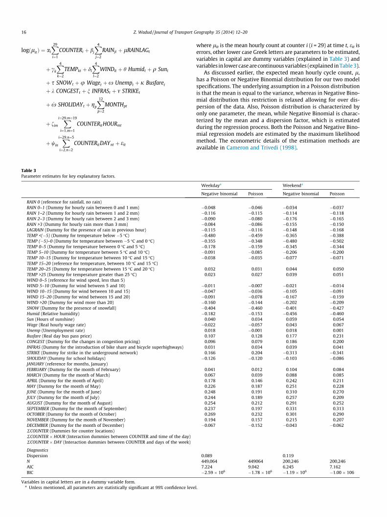
where lit is the mean hourly count at counter i (i = 29) at time t, eit iserrors, other lower case Greek letters are parameters to be estimated,variables in capital are dummy variables (explained in Table 3) andvariables in lower case are continuous variables (explained in Table 3).

As discussed earlier, the expected mean hourly cycle count, l,has a Poisson or Negative Binomial distribution for our two modelspecifications. The underlying assumption in a Poisson distributionis that the mean is equal to the variance, whereas in Negative Bino-mial distribution this restriction is relaxed allowing for over dis-persion of the data. Also, Poisson distribution is characterized byonly one parameter, the mean, while Negative Binomial is charac-terized by the mean and a dispersion factor, which is estimatedduring the regression process. Both the Poisson and Negative Bino-mial regression models are estimated by the maximum likelihoodmethod. The econometric details of the estimation methods areavailable in Cameron and Trivedi (1998).

Weekdaya Weekenda

Negative binomial Poisson Negative binomial Poisson

�0.048 �0.046 �0.034 �0.037�0.116 �0.115 �0.114 �0.118�0.090 �0.080 �0.176 �0.165�0.084 �0.086 �0.155 �0.150�0.115 �0.116 �0.148 �0.168�0.480 �0.459 �0.365 �0.388�0.355 �0.348 �0.480 �0.502�0.178 �0.159 �0.345 �0.344�0.091 �0.085 �0.206 �0.200�0.038 �0.035 �0.077 �0.071

0.032 0.031 0.044 0.0500.023 0.027 0.039 0.051

�0.011 �0.007 �0.021 �0.014�0.047 �0.036 �0.105 �0.091�0.091 �0.078 �0.167 �0.159�0.160 �0.144 �0.202 �0.209�0.404 �0.460 �0.401 �0.427�0.182 �0.153 �0.456 �0.460

0.040 0.034 0.059 0.054�0.022 �0.057 0.043 0.067

0.018 �0.001 0.018 0.0010.107 0.128 0.177 0.2310.096 0.079 0.186 0.2000.031 0.034 0.039 0.0410.166 0.204 �0.313 �0.341�0.126 �0.120 �0.103 �0.086

0.041 0.012 0.104 0.0840.067 0.039 0.088 0.0850.178 0.146 0.242 0.2110.226 0.187 0.251 0.2280.248 0.191 0.310 0.2700.244 0.189 0.257 0.2090.254 0.212 0.291 0.2520.237 0.197 0.331 0.3130.269 0.232 0.301 0.2900.194 0.157 0.215 0.207�0.067 �0.152 �0.043 �0.062

0.089 0.119449,064 449064 200,246 200,2467.224 9.042 6.245 7.162�2.59 � 106 �1.78 � 106 �1.19 � 106 �1.00 � 106

l.

Z. Wadud / Journal of Transport Geography 35 (2014) 12–20 17

Our literature review suggests that the sensitivity to rainfall,wind or temperature for commuting or utilitarian and recreationaltravel can be different. We hypothesize that weekday travel is gen-erally utilitarian and weekend travel is for leisure and thereforerun two separate models for weekdays and weekends to test ifthe parameter estimates are indeed different. We also include pub-lic (bank) holidays in the weekend model, specifically, as havingthe flow characteristics of a Sunday.

Fig. 3. Estimates for days of the week (weekdays) dummies (win) for differentcounters.

4. Results

4.1. Cycling count model

Estimation results for weekdays and weekends are presented inTable 3, for Negative Binomial and Poisson regression. The statisti-cal test on the choice between a Negative Binomial and Poissonmodel hinges on the significance of the dispersion parameter inthe Negative Binomial model: if it is different from zero, thenNegative Binomial model is preferred. We indeed find that thedispersion parameter is statistically different from zero at 99% con-fidence level. Therefore we opt for the Negative Binomial model.

We include the results for monthly dummies in the Table 3, butomit the parameter estimates for the dummy variables for individ-ual counters and hourly and day of week interactions with coun-ters for the sake of brevity (full parameter estimates are availableon request). These parameters are plotted in Figs. 2 and 3 graphi-cally. Three different patterns of hourly bicycle flows are high-lighted (thick lines) for three representative counter locations inFig. 2. Most of the locations show two peaks, but even among thosethere are substantial differences in the relative magnitudes, justify-ing our approach of interacting counter locations with hours.

The differences between daily patterns in a week are not aslarge as the hourly differences (Fig. 3). Except for one counter(No. 173) all the counters show a similar non-linear daily cycleflow pattern: slight increases during Tuesdays and Wednesdaysas compared to Mondays and then dropping off significantly on Fri-days. Total daily flows during Saturdays and Sundays are evensmaller (although they cannot be plotted on the same graph dueto differences in the scale of two models), with Sundays and publicholidays showing the smallest cycle flows (from weekend modelresults). Note that our model has a semi-logarithmic functionalform, therefore the parameter estimates are not the traditionalelasticities. Also, the parameter estimates between the counterscannot be used to directly compare the absolute flow characteris-tics between counters.

The weekday model supports previous assertion that rain ad-versely affects cycling flows, with maximum reduction taking

Fig. 2. Estimates for hourly flow dummies (fim) for different counters.

place for hourly rains between 1 and 2 mm in our case. A substan-tial and statistically significant lagged effect of rain is also clearlyvisible. An increase in temperature increases bicycle usage, butthe increase is non-linear and levels off (or slightly decreases) attemperatures above 25 �C. Higher wind speed reduces cyclingflows, with the effect nearly linear. Presence of snow has the larg-est impact on cycling, with a reduction of around 40% in weekdayflows. An increase in humidity reduces bicycle use, while an in-crease in sunshine hours increases its use – although both effectsare statistically significant, the absolute effects are not substantial.

A comparison of the weekday and weekend model reveals inter-esting insights. In general, the impact of weather is larger in theweekend model, which supports the hypothesis that leisure travelis more sensitive to weather events than utilitarian cycling. How-ever, while this effect is pronounced at heavier rains, light raindoes not deter leisure cycling more than utilitarian cycling. Effectof temperature is consistently larger for leisure cycling, with anaberration at very low temperatures (which is possibly spurious).Snow has similar effect on weekday and weekend cycling, buthumidity has a substantially larger effect on weekend cyclingflows.

During weekdays, an increase in the real hourly wage rate re-duces bicycle flows (2.18% for every GBP increase), hinting thatutilitarian cycling could be an ‘inferior’ good, although this hypoth-esis requires further investigation using other measures of income.An increase in unemployment rate also increases cycling flow dur-ing weekdays by 1.82%. Cycling flows during weekdays in Londonincreases substantially with an increase in bus fares (by 11.3% forevery GBP increase), an increase in the congestion charge to centralLondon (by 10% in January 2011 price hike) or a strike in the under-ground rail network (by 18.1% during strike days), all of which re-veals cycling as a substantial substitute transport mode in London.The effects of wage rate, unemployment, bus fare and congestioncharge together partially explain the increase in bicycle usage inLondon during 2008–2011 period. In comparison, the opening ofthe cycle hire and the two bicycle superhighways had a relativelymodest association with the increase of bicycle flows (3.15% in July2011), although the longer term impact, which would require alonger time series of data to investigate, could be larger. Also ourtime series is small (only 4 years) to decipher any longer term pro-pensity toward increased cycling – therefore the parameter esti-mates for wage rate and unemployment should be treated withcare, as they might reflect the effect of time too.

The weekend model shows similar direction of impacts as in theweekday model, with two differences. An increase in wage rate in-crease bicycle flows, indicating leisure cycling as a normal good.The effect of strike on the tube network has a negative impact on

(a) (b)Fig. 4. Distribution of changes in bicycle flows for 100 plausible weather patterns in 2041, with respect to (a) 2011 and (b) 2009 baseline.

18 Z. Wadud / Journal of Transport Geography 35 (2014) 12–20

weekend cycling. Given the travel chaos a strike brings about, it ispossible that people simply forego their leisure travel during thestrike days generating the negative impact on weekend cycling.

Fig. 5. Percent change in bicycle flows due to climate change during weekdays andweekends for different seasons.

1 The difference in 2041 flows for the two baseline scenarios of 2009 and 2011 isue to the differences in the number of school holidays, which we kept constant forach set of baseline and future projections.

4.2. Future projected cycling

4.2.1. Average effectsProjected future weather pattern under a changed climate sce-

nario for 2041 is fed into the hourly bicycle count model to get pro-jected bicycle count in 2041. Given some of the variables (snow,wind speed) are not available from the UKCP 09, these variablesare kept at the base year values. We use year 2011 as our base year,which is the latest available data for our count model. However, in-stead of directly using 2011 cycle counts as our base dataset forcomparison, we use predicted bicycle count from the econometricmodel for year 2011. We use the predictions for our baseline cyclecounts in order to overcome the missing data in some of the coun-ters. This results in an annual average hourly cycle count of 39.81(95% confidence interval 39.58–40.04) in the TLRN network.

Given we have 100 simulations of future hourly weather pat-terns, we also have 100 projected hourly counts for each hour ofthe year. The annual average of these 100 mean hourly bicyclecounts is 40, with 95% confidence interval between 39.98 and40.02. This is a difference of only 0.5% from the baseline weatherscenario of 2011, which is not statistically significant at 95% confi-dence (although significant at 90%). The primary reason for the rel-atively modest change is the counteracting effects of rain andtemperature, as found by Bocker et al. (2013b) as well. A projectedincrease in temperature increases future bicycle use, but an in-crease in rainfall tempers the effect. Especially, 2011 was the driestand the warmest of the four years for which we have our cyclecount data, therefore the projected changes were the smallest.

A further look into the annual average bicycle count for eachplausible weather pattern shows a range of an increase of 2.6% toa reduction of 2.5%. Around 20% of the plausible weather patternsresult in a possible reduction in flow, albeit most of it marginal.Fig. 4(a) presents the frequency distribution of the changes in an-nual average hourly cycle flows for the 100 plausible future weath-er patterns.

Since the change is sensitive to the base year conditions, we alsotest the future flows with respect to another base year, 2009. Year2009 was wetter and colder than 2011, which would hint that theincrease in future cycle flows with respect to 2009 will be furtherincreased. This is indeed the case, as we find the baseline predic-tion for 2009 to be 38.15 per hour while the future projected flow

is 38.84 per hour on average, indicating a 1.7% increase, which isstatistically significant as well.1 Fig. 4(b) presents the distributionof changes for this case, which shows larger increases than Fig4(a). The frequency distribution also shows that in only 3 cases therewere no increases in cycling flows in 2041 with respect to the flow in2009; and the range of change varies from �1.3% to +3.9%.

4.2.2. Seasonal and weekly effectsThe changes in the weather pattern due to climate change are

not constant throughout all seasons. Since the weather patternsduring different seasons get affected differently, the seasonalchanges in the cycle flows are also expected to be different in achanged climate. The fine temporal resolution in our count model-ling framework easily allows us to decipher the differences in sea-sonal changes in the cycling flows due to climate change.Modelling results show that cycling flows increase by 1.5% in thewinter and 2.5% during the summer over year 2011 baseline(Fig. 5). However, these increases are countered by a reduction of2.0% and 0.1% during the spring and autumn respectively, resultingin a net annual hourly increase of 0.5%, as mentioned earlier.

Disaggregating the seasonal patterns further into weekdays(representing utilitarian cycling) and weekends (representing lei-sure cycling), we again find differential impacts. During the winter,

de

Z. Wadud / Journal of Transport Geography 35 (2014) 12–20 19

weekday bicycle counts increase more than the weekend bicyclecounts (1.61% vs. 1.1%). The differences between the climate in-duced changes in cycling flows during the weekends and weekdaysis the least prominent during the spring, when they are reduced by2.25% and 2% respectively. On the other hand, the Summer monthsshow a large variation: weekday flows increase by 1.6%, but week-end (and holidays) flows increase by 7%. During the autumn, week-day flows show a slight reduction (0.35%) but weekend flowsincrease by 1%, with a negligible change in the combined impact.On an annual hourly average basis, weekday bicycle flows increaseby only 0.17%, while weekend flows increase by 1.97%. All of theseseasonal and weekly changes are calculated on the basis of a 2011baseline, and a 2009 baseline would most likely show even largerincreases.

5. Conclusions

The use of bicycle as a transport mode or a leisure activity isparticularly affected by the different elements of daily weather,which is expected to change considerably in the future becauseof the climate change. The objective of this paper was to developa framework that could be used to determine the impact of climateinduced changes in future weather pattern on bicycle flows andapply that framework to London which has seen a rapid growthin cycling in the past decade. We developed a bicycle count modelfor London and employed the UKCP 09 modelling results for futureclimate change to understand the potential changes in bicycle flowin 2041, with respect to those in 2011. To our knowledge, this isthe first study to utilize an hourly resolution future weather data,downscaled from the GCMs, to study the effect of climate changeon bicycle use. In order to capture the potential uncertainty infuture climate change and the associated weather patterns, we alsosimulate 100 plausible weather patterns under a changed climate,which is a different approach from the existing studies which usesingle values for the annual changes in the weather. Our bicyclecount model for London supports previous findings that bicycleflow is indeed sensitive to the weather, with leisure cycling moresensitive than the utilitarian one. We also found evidence that util-itarian cycling could decrease as a result of higher income or lowerunemployment rate which could potentially lead to lower cyclingfor commuting when the UK economy gains momentum in thefuture.

Bicycle flow in London is expected to increase due to the cli-mate change, although the magnitude of this increase is modest,even in the high emissions scenario of UKCP 09. Given the hightemporal resolution of our count model, the projected relativechanges in future bicycle flows are sensitive to the choice of thebaseline year. By 2041, bicycle flows are expected to increase dur-ing the summer and the winter, but the reductions in the springand the autumn temper the net annual effect. The largest increase(�7% over year 2011 baseline) in bicycle use is during the week-ends of the summer months for leisure travel. This would poten-tially result in better utilization efficiency of the bicycleinfrastructure during the summer off-peak periods. The maximumincrease in daily weekday travel is 1.6% during the summer and thewinter, which is not very large. Still, even this small increase can beimportant if the future bicycle network gets congested – a possibil-ity during the summer months – as it can result in a more than pro-portional increase in travel delay.

Care must be exercised in interpreting our results. Longer runcycling flows depend on a number of other, possibly more influenc-ing variables than weather, e.g. policy and safety initiatives, newtechnologies or prices of fuel and alternate transport modes, etc.Also there could be substantial changes in the perception about cy-cling and related behavioural traits over the next few decades. Our

model thus is more appropriate in answering the question whathappens if we have a changed weather pattern due to climatechange now, rather than what happens in general in the future.Nonetheless, the relative impacts on cycle flows from our modelwill remain valid as long as people’s sensitivity to the weather vari-ables do not change, although the absolute flow levels may not.

There are a few data limitations too. The weather model cannotpredict snowfall, which has a large hourly impact on the cycle flow.Given the general increase in temperature due to climate change, itis likely that snowfall will be reduced. Our results therefore pro-vide the lower bound of the potential increases in the bicycle flow.Although we could not incorporate changes in wind speed too, re-cent results of UKCP 09 show that future changes in wind speedand thus its effect on our results is negligible. Our model also doesnot incorporate the impacts of extreme weather induced events,e.g. bike path or bike lane closures due to flooding resulting fromexcessive rainfall, which can be important for climate adaptationplanning. This would require a different modelling approach, pos-sibly in the area of asset management. Also, our results cannot begeneralized to every other region in the world since the changes inweather pattern due to a changed climate and the sensitivity ofbicycle use to temperature and rainfall will be different spatially.However, the modeling framework can be applied universallysubject to the availability of the underlying data.

Acknowledgement

The author thanks Transport for London (TfL) for providing thedata from the automated bicycle counters for London.

References

Ahmed, F., Rose, G., Jacob, C., 2010. Impact of weather on commuter cyclistbehaviour and implications for climate change adaptation, 33rd AustralasianTransport Research Forum, Canberra.

Ahmed, F., Rose, G., Figliozzi, M., Jakob, C., 2012. Commuter cyclists sensitivity tochanges in weather: Insights from two cities with different climatic conditions.In: 91st Annual Meeting of the Transportation Research Board, January,Washington, DC.

Bergstrom, A., Magnussen, R., 2003. Potential of transferring car trips to bicycleduring winter. Transp. Res. Part A 37, 649–666.

Bocker, L., Dijst, M., Prillwitz, J., 2013a. Impact of everyday weather on individualdaily travel behaviours in perspective: a literature review. Transp. Rev. 33 (1),71–91.

Bocker, L., Prillwitz, J., Dijst, M., 2013b. Climate change impacts on mode choicesand travelled distance: a comparison of present with 2050 weather conditionsfor the Randstad Holland. J. Transp. Geogr. 28, 176–185.

Brandenburg, C., Matzarakis, A., Arnberger, A., 2007. Weather and cycling – a firstapproach to the effects of weather condition on cycling. Meteorol. Appl. 14, 61–67.

Buehler, R., Pucher, J., 2012. Cycling to work in 90 large American cities: newevidence on the role of bike paths and lanes. Transportation 39, 409–432.

Cameron, A.C., Trivedi, P.K., 1998. Regression Analysis of Count Data. CambridgeUniversity Press, Cambridge.

Cervero, R., Duncan, M., 2003. Walking, bicycling and urban landscapes: evidencefrom the San Francisco Bay Area. Am. J. Public Health 93 (9), 1478–1483.

DEFRA (Department for Environment, Forrest and Rural Affairs), 2013. UK ClimateImpact Project 2009, <http://ukclimateprojections.defra.gov.uk/> (accessed02.02.13).

Dill, J., Carr, T., 2003. Bicycle commuting and facilities in Major US cities: If youbuild them, commuters will use them – another look. In: 82nd Annual Meetingof the Transportation Research Board, Washington, DC.

ECF (European Cyclists’ Federation), 2011. Cycle more often 2 cool down the planet:Quantifying CO2 savings of cycling, Brussels.

Emmerson, P., Ryley, TJ., Davies, DG., 1998. The impact of weather on cycle flows.Traffic Eng. Control.

Flynn, B.S., Dana, G.S., Sears, J., Aultman-Hall, L., 2012. Weather factor impacts oncommuting to work by bicycle. Prev. Med. 54, 122–124.

Gebhart, K., Noland, R.B., 2013. The impact of weather conditions on capitalbikeshare trips. In: 92nd Annual meeting of the transportation research board,January 13–17, Washington, DC.

Goetzke, F., Rave, T., 2011. Bicycle use in Germany: explaining differences betweenmunicipalities through network effects. Urban Stud. 48 (2), 427–437.

Greater London Authority, 2013. Unemployment rate, region, <http://data.london.gov.uk/datastore/package/unemployment-rate-region> (accessed17.05.13).

20 Z. Wadud / Journal of Transport Geography 35 (2014) 12–20

Hanson, S., Hanson, P., 1977. Effects of weather on bicycle travel. Transp. Res.Record 629, 43–48.

Heinen, E., Maat, K., van Wee, B., 2011. Day-to-day choice to commute or not bybicycle. Transp. Res. Record: J. Transp. Res. Board. 2230, 9–18.

Keay, C., 1992. Weather to cycle, Ausbike 92. In: Proceedings of a national bicycleconference, Melbourne, pp. 152–155.

Koetse, M.J., Rietveld, P., 2009. The impact of climate change and weather ontransport: an overview of empirical findings. Transp. Res. Part D 14, 205–221.

Miranda-Moreno, LF., Nosal, T., 2011. Weather or not to cycle: temporal trends andimpact of weather on cycling in an urban environment. Transp. Res. Record: J.Transp. Res. Board 2247, 42–52.

Nankervis, M., 1999. The effect of weather and climate on bicycle commuting.Transp. Res. Part A 33, 417–431.

ONS (Office for National Statistics) 2013a. Consumer Price Indices time series datatable, <http://www.ons.gov.uk/ons/rel/cpi/consumer-price-indices/april-2013/cpi-time-series-data.html>, (accessed 01.05.13).

ONS (Office for National Statistics) 2013b. Regional Economic Analysis, Changes inreal earnings in the UK and London, 2002 to 2012, <http://www.ons.gov.uk/ons/rel/regional-trends/regional-economic-analysis/changes-in-real-earnings-in-the-uk-and-london–2002-to-2012/index.html>, (accessed 01.05.01).

Parkin, J., Wardman, M., Page, M., 2008. Estimation of the determinants of bicyclemode share for journey to work using census data. Transportation 35 (1), 93–109.

Phung, J., Rose, G., 2007. Temporal variations in usage of Melbourne’s bike paths,30th Australasian Transport Research Forum, Melbourne.

Pooley, C., Horton, D., Scheldman, G., Tight, M., Harwatt, H., Jopson, A., Jones, T.,Chisholm, A., Mullen, C., 2010. Can increased walking and cycling reallycontribute to the reduction of transport-related carbon emissions? In: RoyalGeographical Society Annual Conference, London.

Pooley, C., Tight, M., Jones, T., Horton, D., Scheldeman, G., Jopson, A., Mullen, C.,Chisholm, A., Strano, E., Constantine, S., 2011. Understanding walking andcycling: summary of key findings and recommendations, Lancaster University.

Pucher, J., Buehler, R., 2006. Why Canadians cycle more than Americans: acomparative analysis of bicycling trends and policies. Transp. Policy 13, 265–279.

Rashad, I., 2009. Associations of cycling with urban sprawl and the gasoline price.Am. J. Health Promotion 24 (1), 27–36.

Richardson, A.J., 2000. Seasonal and weather impacts of urban cycling trips, TUTIReport 1-2000, The Urban Transport Institute, Victoria.

Sabir, M., 2011. Weather and travel behaviour, PhD Dissertation, Vrije Universiteit,Amsterdam.

Saneinejad, S., Roorda, M.J., Kennedy, C., 2012. Modelling the impact of weatherconditions on active transportation travel behaviour. Transp. Res. Part D 17,129–137.

Smith, M.S., Kauermann, G., 2011. Bicycle commuting in Melbourne during the2000s energy crisis: a semiparametric analysis of intraday volumes. Transp. Res.Part B 45, 1846–1862.

Thomas, T., Jarsma, R., Tutert, 2013. Exploring temporal fluctuations of daily cyclingdemand on Dutch cycle paths: the influence of weather on cycling.Transportation 40, 1–22.

Tin, S.T., Woodward, A., Robinson, E., Ameratunga, S., 2012. Temporal, seasonal andweather effects on cycle volume: an ecological study. Environ. Health 11 (12),1–9.

Transport for London, 2012. Transport for London’s written submission to theLondon Assembly Transport Committee’s investigation into cycling in London,<http://www.london.gov.uk/sites/default/files/TfL-Written-Submissions-cycle-evidence.pdf>, (accessed 11.05.13).

UK Government, 2013. Policy: Adapting to climate change, <https://www.gov.uk/government/policies/adapting-to-climate-change>, (accessed 25.05.13).

UK Meteorological Office, 2011. Climate: observations, projections and impacts,crown copyright.

UK Meteorological Office, 2013. Met Office Integrated Data Archive System (MIDAS)Land and Marine Surface Stations Data (1853-current). NCAS BritishAtmospheric Data Centre, <http://www.badc.nerc.ac.uk/view/badc.nerc.ac.uk__ATOM__dataent_ukmo-midas>, (accessed 03.01.13).

UK Parliament, 2013. Daily Hansard-Written Answers, 15 June 2011, <http://www.publications.parliament.uk/pa/cm201011/cmhansrd/cm110615/text/110615w0002.htm#11061561000164>, (accessed 31.03.13).

UKCIP (UK Climate Impact Programme), 2011. Preparing for climate change:adapting local transport, Oxford.

Wardman, M., Tight, M., Page, M., 2007. Factors influencing the propensity to cycleto work. Transp. Res. Part A 41, 339–350.

Winters, M., Friesen, MC., Koehoorn, M., Teschke, 2007. Utilitarian bicycling: amultilevel analysis of climate and personal influences. Am. J. Prev. Med. 32, 52–58.

Wittink, R., 2010. Cycling and the Climate Agenda. Interface for Cycling Expertise,Netherlands.