DAMAGE EVOLUTION IN UNIAXIAL SiC FIBER

REINFORCED Ti MATRIX COMPOSITES

Thesis by

Jay Clarke Hanan

In Partial Fulfillment of the Requirements

for the Degree of

Doctor of Philosophy

California Institute of Technology

Pasadena, California

2002

(Defended June 18, 2002)

ii

© 2002

Jay Clarke Hanan

All Rights Reserved

iii

Acknowledgments

Several people have been helpful in bringing me to this point. The top of my list is

clearly occupied by Robin. She is much more than my wife exemplifying the noble

character many others never achieve. Of course, when considering family, I must be

grateful to my parents Russ and Jan who continually encouraged creativity.

It was my undergraduate physics professor and academic advisor, Dr. Lynn

Feuerhelm, who encouraged me to consider graduate school. I would not be here

without him or the fateful meeting of John Rousseau who like so many other members

of the Caltech community represented it favorably to a receptive undergrad looking for

the right opportunity.

Dr. Ersan Üstündag has been extremely helpful as my academic and research

advisor. He took a chance with me as I did with him, being his first student. Even

though we have not agreed on everything, we would agree the chance was worth it. He

always considered my opinion and was so instrumental in getting us to this point,

which when I started down this path five years ago seemed far away. Looking back

through this now seemingly short time, we have both grown first in science and never

least in friendship. It was Dr. Üstündag’s contacts, including

Bjørn Clausen of LANSCE at Los Alamos National Lab who was

extremely helpful with the FEM work; irreplaceable Dr. I. Cev Noyan of

the IBM Watson Research Center who was such an inspiration

contributing valuable advice and resources (including his load frame); Jon

Almer and Ulrich Linert of the APS who helped facilitate the majority of

iv the relevant data collection and analysis; and Irene Beyerlein, also from

Los Alamos, providing support with the micromechanical modeling,

which helped make up the army of people necessary to complete this work. There were

also several graduate students who were helpful during the experiments where we not

only tested materials, but ourselves (especially after sleep deprivation), namely: Geoff

Swift, Stefen Kaldor, and Can Aydiner. I also have to thank Kevin Foltz who along

with my sister Rae and daughter Raevan unknowingly challenged me to finish sooner

rather than later.

I am also grateful to Dr. H. Deve at 3M Corp. for providing the specimens and

helpful discussions about the properties of Ti-SiC composites. This study was

supported by the National Science Foundation (CAREER grant no. DMR-9985264) at

Caltech and a Laboratory-Directed Research and Development Project (no. 2000043) at

Los Alamos. The work at the Advanced Photon Source was supported by the U.S.

Department of Energy, Office of Basic Energy Sciences (contract no. W-31-109-ENG-

38).

v

Abstract

Damage Evolution in Uniaxial SiC Fiber Reinforced Ti

Matrix Composites

by Jay Clarke Hanan

Fiber fractures initiate damage zones ultimately determining the strength and

lifetime of metal matrix composites (MMCs). The evolution of damage in a MMC

comprising a row of unidirectional SiC fibers (32 vol.%) surrounded by a Ti matrix was

examined using X-ray microdiffraction (µm beam size) and macrodiffraction (mm

beam size). A comparison of high-energy X-ray diffraction (XRD) techniques

including a powerful two-dimensional XRD method capable of obtaining powder

averaged strains from a small number of grains is presented (HEµXRD2).

Using macrodiffraction, the bulk residual strain in the composite was determined

against a true strain-free reference. In addition, the bulk in situ response of both the

fiber reinforcement and the matrix to tensile stress was observed and compared to a

three-dimensional finite element model. Using microdiffraction, multiple strain maps

including both phases were collected in situ before, during, and after the application of

tensile stress, providing an unprecedented detailed picture of the micromechanical

behavior in the laminate metal matrix composite.

Finally, the elastic axial strains were compared to predictions from a modified shear

lag model, which unlike other shear lag models, considers the elastic response of both

constituents. The strains showed excellent correlation with the model. The results

confirmed, for the first time, both the need and validity of this new model specifically

vi developed for large scale multifracture and damage evolution simulations of metal

matrix composites. The results also provided unprecedented insight for the model,

revealing the necessity of incorporating such factors as plasticity of the matrix, residual

stress in the composite, and selection of the load sharing parameter.

The irradiation of a small number of grains provided strain measurements

comparable to a continuum mechanical state in the material. Along the fiber axes,

thermal residual stresses of 740 MPa (fibers) and +350 MPa (matrix) were found.

Local yielding was observed by 500 MPa in the bulk matrix of the composite. Plastic

anisotropy was observed in the matrix. The intergranular strains in the Ti matrix varied

as much as 50%. In spite of this variation, the HEµXRD2 technique powerfully

provided reliable information from the matrix as well as the fibers.

vii

Table of Contents

Acknowledgments .............................................................................................. iii

Abstract ................................................................................................................ v

Table of Contents .............................................................................................. vii

List of Illustrations and Tables........................................................................... ix

1. Introduction ............................................................................................... 21

1-1. Background and Motivation .......................................................................... 21

1-2. Approach........................................................................................................ 26

2. Diffraction Techniques to Study Composites .......................................... 28

2-1. Strain and X-Ray Diffraction......................................................................... 28

2-1.1. Strain Measurements with In Situ Mechanical Loading........................ 32

2-2. High-Resolution X-Ray Strain Measurements. ............................................. 36

3. Two-Dimensional Fiber Composite Models ............................................ 51

3-1. A Finite Element Model for Ti-SiC............................................................... 51

3-2. A Micromechanics Model for Damaged Ti-SiC............................................ 56

3-2.1. Matrix Stiffness Shear Lag (MSSL) Model........................................... 58

4. Bulk Deformation of Ti-SiC Composites................................................. 69

4-1. The Ti-SiC Composite ................................................................................... 69

4-2. X-Ray Diffraction Method............................................................................. 73

4-3. Mechanical Loading ...................................................................................... 78

4-4. Bulk Residual Strains in the Composite ........................................................ 80

4-5. Bulk Applied Strains...................................................................................... 83

4-6. Bulk Residual Strain Evolution ..................................................................... 93

viii 4-7. Conclusions on the Bulk Laminate Properties............................................... 96

5. Microscale Deformation of Ti-SiC Composites ...................................... 97

5-1. Controlled Damage in Ti-SiC Composites .................................................... 97

5-2. Additional Residual Strain Measurements in Ti-SiC Composites............... 103

5-2.1. “sin2ψ” Experimental Procedure ......................................................... 106

5-2.2. “sin2ψ” Results and Discussion ........................................................... 110

5-2.3. “sin2ψ” Conclusions ............................................................................ 114

5-3. Microbeam Diffraction Method................................................................... 115

5-4. Microscale Residual Strains......................................................................... 126

5-5. Microscale Load Sharing ............................................................................. 143

5-6. Residual Strain Evolution in the Microscale ............................................... 158

5-7. Comparison with Matrix Stiffness Shear Lag Model .................................. 171

6. Conclusion............................................................................................... 191

6-1. General Conclusions .................................................................................... 191

6-2. Future Work................................................................................................. 194

7. Appendices .............................................................................................. 197

7-1. Appendix A. Load Frame and Strain Gage Interface Code........................ 197

7-2. Appendix B. Image Plate Calibration and Conversion Macro ................... 202

7-3. Appendix C. Image Plate Analysis Code.................................................... 204

References................................................................................................................ 214

ix

List of Illustrations and Tables

Figures Number Page

Figure 1-1 Some example views of continuous fiber metal matrix composites........... 22

Figure 2-1 Photograph of adapted Fullam load frame on the goniometer at the 7.3.3 microdiffraction beam line at the Advanced Light Source. In this orientation, the open face of the load frame allows X rays to reflect from the surface of the sample. ................................................................................................................... 33

Figure 2-2 Schematic of the diffracted beam position and the position of receiving slits. ........................................................................................................................ 36

Figure 2-3 (a) Scattering geometry of a synchrotron experimental setup. x, y, z define the laboratory coordinate system, z being parallel to the incident beam, x is in the horizontal plane pointing outwards from the storage ring, and y is perpendicular to both z and x. The scattering vector q and the diffracted beam for a diffracting grain are indicated by solid arrows. Note that all scattering vectors coinciding on a cone with large opening angle (indicated by the dashed scattering vectors) are detected simultaneously on an area detector........................................................................ 40

Figure 2-4 Diffraction patterns constructed from a θ/2θ scan with an analyzer crystal at 25 keV (left) and using a strip of pixels along η = 0 from an image plate exposure at 65 keV (right). Notice the peaks are much narrower with fewer data points, marked by an “o,” in a peak using the analyzer crystal, but the image plate scan takes less than 1/8th the time and includes information from all η. (See Section 4-2 for a fully indexed pattern.) ................................................................................ 41

Figure 2-5 The image plate, initially exposed with rings in a radial format (left), is converted to a Cartesian format (right) for analysis. ............................................. 46

Figure 2-6 A zoomed-in view from two exposures of the image plate on the Ti-SiC laminar composite (see Figure 2-5 for coordinates). The first (top) is at 0 MPa applied stress, the second at 850 MPa. Axial strains appear as shifts between the two frames directly at η = 0o, 180o and 360o. Transverse strains are visible at η = 90o and 270o. For all other η the strain is a combination...................................... 49

Figure 2-7 The translation error vs. applied load corrected for in the Ti-SiC composite. An internal Si standard powder on the composite surface provided this information............................................................................................................. 50

Figure 3-1 Finite element model (FEM) geometry and predictions of elastic strains at 650 MPa applied composite stress (along fiber axis, i.e., the z direction). (a) Mesh used in the FEM calculations. (b), (c) and (d) Normal strain distributions along the x, y and z directions, respectively. In (b) and (c), significant transverse strain gradients are observed across the specimen thickness. There is no variation in the

x longitudinal elastic strain in the fiber (d), but there is some variation in the matrix due to predicted plastic deformation around the fiber. Average longitudinal strains in the fibers due to the applied stress alone are around 3040 µε while they are about 3110 µε in the matrix.. ................................................................................. 53

Figure 3-2 A representative finite element mesh from the MSSL model for a laminar fiber composite (adapted from [34]). ..................................................................... 59

Figure 3-3 Schematic of crack geometries under consideration (adapted from ref. [34]). (a) Case (i): two fibers are broken but the crack-tip matrix regions are intact. (b) Case (ii): in addition to two broken fibers, the crack-tip matrix regions are also broken. Components are numbered with index “n”............................................. 60

Figure 3-4 a) Case (i), and case (ii) with ρ = 0.289 for both one and two broken fibers. b) Comparison of each predicted relative strain value for each ρ value assuming two fiber breaks and case (ii). Under case (ii) for the first intact fiber next to the break εf/ε is greatest for ρ = 0.591, while it is least for ρ = 0.289. c) Under case (i) for the first intact fiber next to the break εf/ε is greatest for ρ = 0.289, while it is least for ρ = 0.591. Case (ii) and (i) refer to strain profiles for fibers with and without failure in the matrix adjacent to the fiber break, respectively. ................. 67

Figure 4-1 Scanning electron microscope (SEM) image of a typical specimen cross section. The fibers are 140 µm in diameter and are almost uniformly spaced with an average center-to-center distance of 240 µm. The carbon core of the SCS-6 fibers is visible as the dark circle in the center of the fibers. Two shades of SiC are also visible in the fiber corresponding to the two stages of SiC growth in manufacturing. The final dark ring around the fiber results from a protective carbon coat applied to the finished fiber. The cracks observed in some fibers occurred during specimen preparation. The total specimen thickness is about 200 µm. The shallow grooves seen in the Ti matrix are a result of the composite processing. ............................................................................................................. 71

Figure 4-2 Schematic showing the composite geometry used in bulk XRD experiments. The composite thickness was 0.2 mm. Fiber positions are represented by white lines within a gray matrix (for illustration only – not to scale). ..................................................................................................................... 72

Figure 4-3 Photograph of the experimental setup used for the 25 keV measurements. The dashed line represents the transmitted and diffracted beam paths. The labels are as follows: (1) receiving slit, (2) Si diode beam stop, (3) translation stage, and (4) φ stage. θ and 2θ rotate about the y axis as shown by the curved arrow. See also Figure 2-3 b. ................................................................................................... 74

Figure 4-4 Indexed diffraction pattern for a θ/2θ scan of the Ti/SiC composite using a 2 x 2 mm2 X-ray beam at 25 keV and a point detector. ........................................ 75

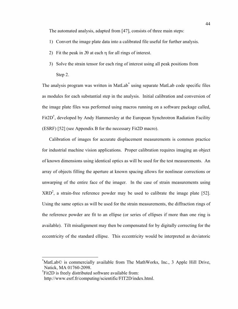
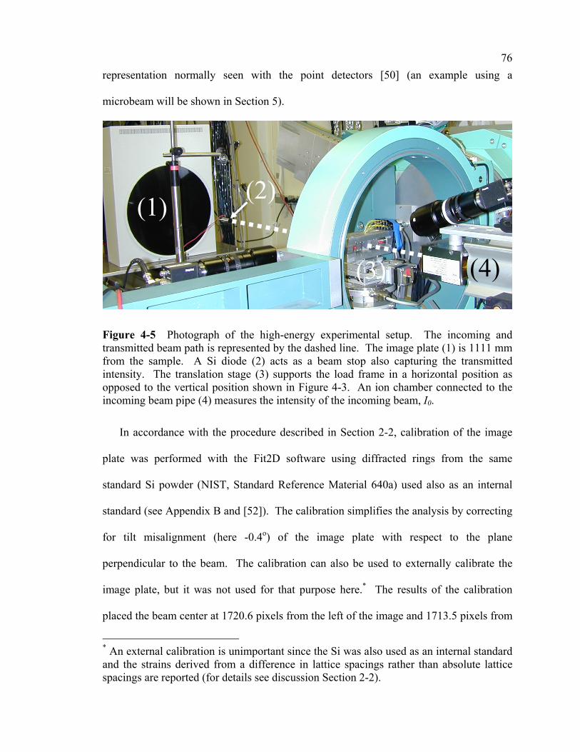
Figure 4-5 Photograph of the high-energy experimental setup. The incoming and transmitted beam path is represented by the dashed line. The image plate (1) is 1111 mm from the sample. A Si diode (2) acts as a beam stop also capturing the transmitted intensity. The translation stage (3) supports the load frame in a

xi horizontal position as opposed to the vertical position shown in Figure 4-3. An ion chamber connected to the incoming beam pipe (4) measures the intensity of the incoming beam, I0. ........................................................................................... 76

Figure 4-6 The strain gage (small circles with a connecting line) reveals drift of strain with time associated with the relaxation of load from a typical constant displacement load step. The strain in the matrix with its associated error given by the least squares refinement is shown by the flat line. Information from the entire 2θ scan (marked by arrows) is included in the refinement. The strains given by the Ti (11.0) and Ti (10.2) is given by the “x” and the “*,” respectively. These along with the strain from the SiC (220) peak, a “o,” are shown at the position the peaks occur in time. ............................................................................................... 79

Figure 4-7 Comparison of experimental strains from bulk with FEM predictions of applied composite stress vs. average elastic axial strains in the first undamaged Ti-SiC composite during a loading/unloading cycle. Strain gage values are shown together with lattice strains in the Ti (10·2), Ti (11·0) and SiC (220) reflections obtained from diffraction. Thermal residual strains are included (see Table 4-1). Note that due to load drifts not every stress level could yield suitable data for Rietveld refinement................................................................................................ 84

Figure 4-8 The macroscopic stress vs. strain in the first loading cycle of the second undamaged composite along the fiber direction according to strain gage data (symbols). Deformation in the composite was elastic up to at least 700 MPa with very little plastic deformation even after 800 MPa. A line from a linear regression fit to the elastic portion of the curve is plotted over the data points to help illuminate the slight deviation from linearity in the strains caused by plastic deformation............................................................................................................ 86

Figure 4-9 Elastic bulk strains in the fiber (a) and matrix (b) for increasing applied tensile stress in the second cycle (symbols) on the second undamaged composite. As before, the stress is applied along the fiber axial direction (axis 1). The FEM prediction for the loading cycle in the composite is also shown (lines). As in Figure 4-7 there is good agreement with the model up to the higher stresses. The deviation near 800 MPa signals the onset of global plastic strain in the matrix. An early onset of plasticity is observed in the transverse (ε22) direction where individual grains naturally show larger variations in strain (see text). (Strains are taken from the matrix (10.2) diffraction ring and the fiber (220) diffraction ring.)............................................................................................................................... 89

Figure 4-10 Strains during the release of applied tensile stress in the second undamaged composite. The arrows show the direction of unloading. The fibers (a) show an overall linear behavior with very little average shear strain over the range of applied stress. However, the matrix (b) appears to deviate from linear behavior particularly in the transverse (ε22) and the shear (ε12) directions............ 91

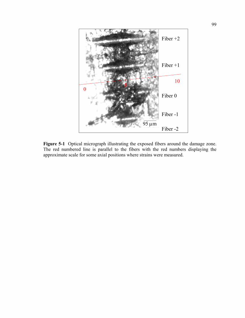
Figure 5-1 Optical micrograph illustrating the exposed fibers around the damage zone. The red numbered line is parallel to the fibers with the red numbers displaying the approximate scale for some axial positions where strains were measured............ 99

xii Figure 5-2 Schematic showing the damaged sample geometry used in the XRD

experiments. The composite thickness was 0.2 mm. Fibers positions are represented by white lines within a gray matrix. The region etched is marked by an oval below the strain gage (for illustration only – not to scale)...................... 100

Figure 5-3 An SEM image at a 45o tilt angle of the hole cut by EDM in the second composite. The hole cut completely through one fiber which was later assigned the label D. Beside it is fiber E which was partially cut. The matrix between these fibers is obviously cut as well as some of the matrix adjacent to D, the completely cut fiber. ............................................................................................................... 102

Figure 5-4 Two photographs of the etched composite during the process of making the strain-free reference (before the fibers were etched away from the matrix). The thermal residual strains are strikingly apparent from this image. Once the fibers were freed from the matrix both phases returned to their originally flat configuration. A razor blade is also shown to provide scale. ............................. 104

Figure 5-5 Diagram of the low-energy microdiffraction technique. 2θ is in the same direction as θ........................................................................................................ 106

Figure 5-6 Contour plot of Ti (20.3) reflection from microdiffraction. The Cu (311) reflection, which is close in d to the Ti reflection, exposes the Cu marker as the rough triangle between grains 13 and 14. The rectangle in the center of the figure borders the region scanned at higher ψ's. ............................................................ 108

Figure 5-7 Comparison of the macrobeam, , and microbeam, x, low-energy measurements....................................................................................................... 112

Figure 5-8 Absorption contrast image of the damaged region in the first composite as captured by the Si diode. Intensity is proportional to absorption, i.e., the darker a region the higher the absorption. The contrast is primarily due to Ti thickness. The low density SiC fibers do not reveal features such as cracks. The absence of matrix from the surface of the sample near the damage region is evidenced by the bright region near the center of the image. The periodic change in intensity along y corresponds to the position of SiC fibers in the matrix. The fibers examined are labeled by number. Matrix regions examined lay between the labeled fibers.... 116

Figure 5-9 Map of β-SiC (220) reflection indicating the location of the buried fibers. The oval outlines the damaged region. Fibers are numbered to indicate their location with respect to the damage zone (at the beginning, “Fiber 0” was broken). It is interesting to note that the 30 x 30 µm2 beam size used in this experiment yielded a continuous map for SiC confirming its small grain size. ..................... 117

Figure 5-10 Map of α-Ti (11.2) reflection indicating the location of diffracting Ti grains. The marked damage zone and fiber locations are visible from the dashed lines available from the transmission data collected simultaneously during the scan. With an average Ti grain measuring 29 µm across, few grains are oriented for diffraction at a given θ angle. The damage zone marked by the arrow was etched to expose fibers......................................................................................... 118

xiii Figure 5-11 The position of diffracting α-Ti grains that contribute to the intensity of

the (10.2) reflection using a 10 x 10 µm2 X-ray beam. Since 9.1 keV X-rays are used, the examined grains are restricted to the surface of the sample. Both sides of the Ti matrix reference specimen were examined so that a layer of grains is exposed at the surface and the midplane of the sample (see Section 5-2 for description of the matrix reference). A photograph of the midplane surface is shown to the left of the contour plot. The layer at the midplane is also marked with what were fiber centers (between the black dashed lines marking the position the fibers were removed from) and matrix centers (between the grey dotted lines). The white horizontal lines are an artifact common to synchrotron analysis. ...... 120

Figure 5-12 A map of the positions sampled for fiber and matrix strains using the image plate method on the second damaged Ti-SiC composite. Each of the 10 fibers was given a label “A” through “J”. Matrix positions are labeled “a” through “i”. A hole was cut in fiber D and its neighborhood using EDM and is marked with an oval. The axial positions at +/-1.43 mm provide information for the far-field strains. Time constraints prevented collecting data from each position on this map. Relevant subsets were examined at each applied stress and are shown separately. ............................................................................................................ 122

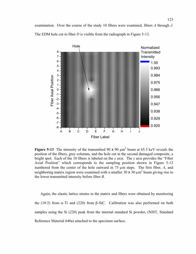
Figure 5-13 The intensity of the transmitted 90 x 90 µm2 beam at 65.3 keV reveals the position of the fibers, grey columns, and the hole cut in the second damaged composite, a bright spot. Each of the 10 fibers is labeled on the x axis. The y axis provides the “Fiber Axial Position” which corresponds to the sampling position shown in Figure 5-12 numbered from the center of the hole outward in 75 µm steps. The first fiber, A, and neighboring matrix region were examined with a smaller 30 x 30 µm2 beam giving rise to the lower transmitted intensity before fiber B. ................................................................................................................. 123

Figure 5-14 Photograph of the load frame mounted on the goniometer in hutch C downstream from 1-BM (bending magnet 1) at APS. The sample with a hole is shown in the grips. See inset (marked by blue rectangle) for a close-up of the composite. Placement of the strain gages is also visible in the image. The Si standard powder is mounted on the upstream side (back side in this image) of the sample. ................................................................................................................. 124

Figure 5-15 The elastic residual strains in the fibers and intervening matrix regions as a function of axial position and fiber number for the damage zone of the first composite. The shade of each square depends on the value of strain measured using the 90 x 90 µm2 beam at that position. Squares containing an “X” denote matrix positions where grains were not favorably oriented for diffraction. The position of the damage zone can be read from the relaxed (near 0) residual strains.............................................................................................................................. 127

Figure 5-16 Example of diffracted peaks obtained from the matrix using the microbeam and a point detector. The weak reflection shown here contributed to an “X” for the cluster of 3 in the upper right corner of Figure 5-15. Its signal to noise is too low for adequate fitting. The background intensity is the same for both peaks. ........................................................................................................... 128

xiv Figure 5-17 Residual fiber axial strain as a function of fiber axial position for the 5

fibers near the etched damage zone in the etched composite. Fiber 0 was broken before applying load. The change in strain for the fibers as a function of axial position is a result of matrix etched from above the fibers. The dashed line shows the strain given by the control fiber far from the damage region. ....................... 129

Figure 5-18 Residual matrix axial strain as a function of fiber axial position for the 4 matrix regions between the 5 fibers examined in the first composite. Both the action of etching away matrix from the surface and breaking the fiber acted to create the observed residual strains. The change in error bar length is associated with the presence or absence of diffracting grains. The strains given by the control matrix region are marked by the dashed lines. .................................................... 131

Figure 5-19 For each fiber examined (D through J), the transmitted intensity measured by a silicon diode divided by the incident intensity measured by an ion chamber is plotted for each axial position sampled along the fiber. The fiber positions are identified by the lighter shade, more transmission, and the thicker matrix regions by the darker shade associated with less transmission. The hole appears the brightest. The axial position spacing is 0.075 mm except for the two extreme “far-field” positions, +/-12, which were an additional 0.6 mm from the previous point (Figure 5-12). ....................................................................................................... 133

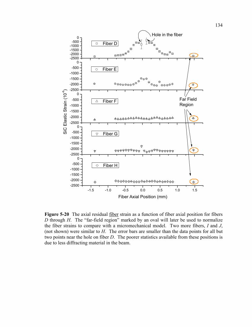
Figure 5-20 The axial residual fiber strain as a function of fiber axial position for fibers D through H. The “far-field region” marked by an oval will later be used to normalize the fiber strains to compare with a micromechanical model. Two more fibers, I and J, (not shown) were similar to H. The error bars are smaller than the data points for all but two points near the hole on fiber D. The poorer statistics available from these positions is due to less diffracting material in the beam. ... 134

Figure 5-21 A contour plot of the matrix axial elastic residual strain for the regions associated with the fibers, marked by the fiber label, and between the fibers. The presence of the hole around axial position 0 diminishes the residual strains in the matrix around fibers D and E. Even at regions distant from the hole, variation is present in the matrix residual strains. Compare spatial resolution with Figure 5-15. ..................................................................................................................... 135

Figure 5-22 The axial residual matrix strain as a function of fiber axial position for the regions between fibers D through J. The effect of cutting the matrix is primarily visible in the matrix between fibers D and E. The other matrix regions show fluctuations in strain, but since they are also observed far from the hole, they were due to possible spatial variations in processing and/or intergranular stress. The image plate clearly improves the ability to observe matrix strain (compare with Figure 5-17). ........................................................................................................ 138

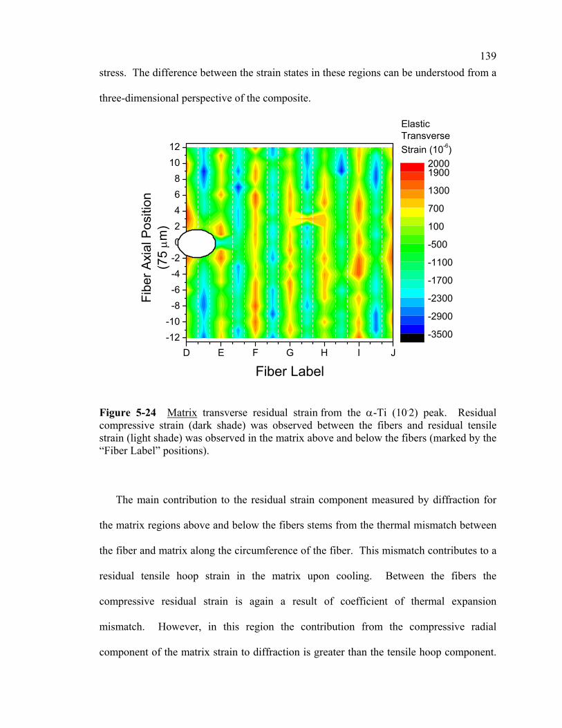
Figure 5-24 Matrix transverse residual strain from the α-Ti (10.2) peak. Residual compressive strain (dark shade) was observed between the fibers and residual tensile strain (light shade) was observed in the matrix above and below the fibers (marked by the “Fiber Label” positions). ............................................................ 139

xv Figure 5-24 a) The FEM prediction from Figure 3-1 with a solid and dashed arrow

along the border of the plot exposing from where the solid and dashed lines for part “b)” were taken. b) Transverse thermal residual strain predicted in the composite by FEM. A center line along the fiber from the midplane of the composite to the surface shows tensile strain in the matrix (solid line). The transverse strains in the matrix centered between the fibers is compressive (dashed line). ..................................................................................................................... 141

Figure 5-25 Damage evolution under tensile load at the crack plane (x = 0 in Figure 5-1). Applied stress is plotted against applied axial lattice strain in the five fibers around the damage zone. At the beginning of loading, only fiber 0 was broken. When the stress/strain profiles of the intact and initially broken fiber are compared, it is obvious that fiber +1 broke between 90 MPa and 430 MPa. ...... 144

Figure 5-26 Applied strain in the first nearest neighbor fiber to the natural break (fiber +2, first damaged composite) for each load as a function of the axial position in the fiber. Load transfer (increase in strain compared to the far-field) from the broken fibers is realized even at the smaller load and continues to increase its magnitude and breath as the load increases. ........................................................ 145

Figure 5-27 Applied strain in fiber +1 which naturally broke while loading the first damaged composite. The fiber shows a clear decrease in strain at the break plane.............................................................................................................................. 146

Figure 5-28 Applied strain in the initially broken fiber as a function of axial position from the break. The wider profile observed in this fiber’s strains compared to the naturally broken fiber are due to the extent of initial damage in the fiber. (Data also from the first damaged composite.).............................................................. 147

Figure 5-29 Similar to fiber +2, the strains in the fiber which was a first nearest neighbor to the initially broken fiber as a function of axial position from the break are shown. The load transfer is first apparent at the smaller applied stress and increases with increasing stress. The profile looses symmetry with the break plane due to the damage profile in its neighbor (Figure 5-28). (Data also from the first damaged composite.) ........................................................................................... 148

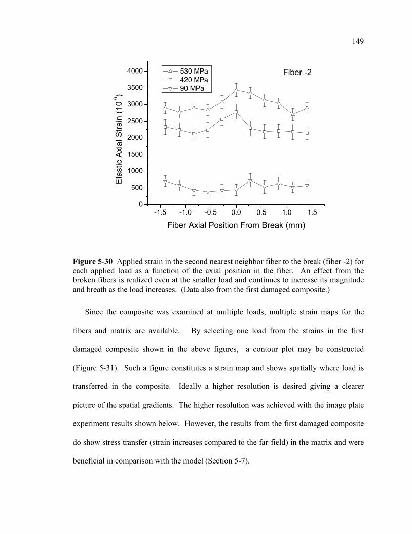
Figure 5-30 Applied strain in the second nearest neighbor fiber to the break (fiber -2) for each applied load as a function of the axial position in the fiber. An effect from the broken fibers is realized even at the smaller load and continues to increase its magnitude and breath as the load increases. (Data also from the first damaged composite.) ........................................................................................... 149

Figure 5-31 Contour plot of the strains at the maximum applied stress (530 MPa) for all the fibers examined in the first damaged composite. The relative position of stress transfer from the break to the intact fibers is clear. The data here is taken from the last applied stress shown in Figure 5-26, Figure 5-27, Figure 5-28, Figure 5-29, and Figure 5-30........................................................................................... 150

Figure 5-32 Each box represents a position analyzed with the 90 x 90 µm2 beam. The fibers A-J and neighboring matrix regions were analyzed in the configuration shown. These positions are a subset of the positions analyzed before stressing the

xvi composite (Figure 5-12). The numeric label for the positions used in the strain contour maps is shown on the right of the figure. For reference, the position of the hole cut in the composite is also shown in the figure. ......................................... 151

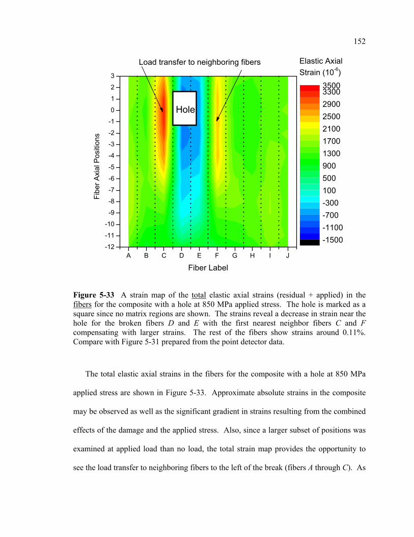
Figure 5-33 A strain map of the total elastic axial strains (residual + applied) in the fibers for the composite with a hole at 850 MPa applied stress. The hole is marked as a square since no matrix regions are shown. The strains reveal a decrease in strain near the hole for the broken fibers D and E with the first nearest neighbor fibers C and F compensating with larger strains. The rest of the fibers show strains around 0.11%. Compare with Figure 5-31 prepared from the point detector data....................................................................................................................... 152

Figure 5-34 The applied axial strains (total strain (Figure 5-33) minus the residual strain (Figure 5-20)) for the fibers D through I are shown for the 850 MPa applied stress. The width of the hole is marked on the graph for fiber D. The spatial resolution and strain resolution have both improved compared to the etched composite previously examined with the point detector. The data point on fiber D taken inside the hole showed less intensity, and therefore a greater error than the other positions...................................................................................................... 153

Figure 5-35 A contour map of the total elastic axial strains in the Ti matrix for the composite with a hole at 850 MPa. The fiber positions are labeled and separated from the “matrix only” columns by dashed grid lines. The broken fibers appreciably affect axial matrix strains two fiber diameters from the break. Such a figure with continuous strain information from the matrix cannot be constructed from the point detector results. ............................................................................ 154

Figure 5-36 A map of the total elastic shear strains in the Ti matrix of the composite with a hole at 850 MPa. The effect of load on the hole is observed in the stress concentrations around the hole. Arrows follow the path of maximum shear away from the hole........................................................................................................ 155

Figure 5-37 A strain map of the total elastic transverse strains in the matrix of the composite with a hole at 850 MPa. The strain at each fiber location is tensile but the strain between each fiber is on average compressive. ................................... 156

Figure 5-38 A typical shift (90 µm) in the axial position of the hole referenced to the laboratory coordinate system due to changing the load on the composite. The transmitted intensity along fiber D normalized by an incoming beam monitor allows alignment in the fiber axial direction. Alignment in the transverse direction may be performed through monitoring the intensity change along the fiber radius (not shown). ......................................................................................................... 159

Figure 5-39 Total matrix axial residual strain around the hole after loading and unloading the composite from 850 MPa. The position of the hole in the composite is marked with an oval. The region marked by the “X” was not sampled due to time constraints. ................................................................................................... 160

Figure 5-40 Matrix transverse residual strain around the hole after loading and unloading the composite from 850 MPa. The position of the hole in the composite

xvii is marked with an oval. The position labeled “X” was not sampled due to time constraints. ........................................................................................................... 161

Figure 5-41 Matrix residual shear strain after loading and unloading the composite from 850 MPa. The position of the hole in the composite is marked with an oval. The arrows connect the points of maximum shear strain traveling away from the hole. As with the plots above, the position labeled “X” was not sampled due to time constraints. ................................................................................................... 162

Figure 5-42 Strain map of the change in matrix axial residual strain due to loading (to 850 MPa) and unloading the second composite. The matrix over the broken fiber, D, is the first column on the left of the map. The darker regions identify locations of greater plastic deformation while loading the composite................................ 164

Figure 5-43 The change in axial residual strain for the first two matrix columns illustrates the contrast between the two regions. Near the plane of the broken fiber significant deformation from the 850 MPa applied stress occurred in the intact matrix column e. Since matrix column d was broken it could not carry load and consequently did not significantly deform near the break................................... 165

Figure 5-44 The significant change in fiber residual axial strain for fiber E, which broke under the application of load. Permanent deformation in the matrix above and below the fiber which deformed as a result of the strain associated with the break is also revealed by the analysis. ................................................................. 166

Figure 5-45 Change in axial strain for fibers D and F. The axial strain does not change near the free surface for the cut fiber D. In contrast, the intact fiber F shows a significant change in residual strain upon unloading due to permanent deformation in the matrix. ........................................................................................................ 167

Figure 5-46 Change in axial strain for the two fibers furthest from the break. Change in the axial matrix strains at these fiber locations is shown as well. ................... 168

Figure 5-47 Change in axial elastic residual strain for fiber G. Though similar to the above fibers far from the break, the position sampled to the immediate negative side of the crack plane showed no change in strain—the sign of a poorly bonded interface. Adding support to the observation, a local increase in plastic deformation was observed at the same location through the change in matrix strain..................................................................................................................... 169

Figure 5-48 Comparison of strains from the MSSL model predictions (case (i) the black line and case (ii) the grey line) and XRD data from fibers (symbols) in the first damaged composite: (a) The two broken fibers; (b) the second intact fiber; (c) first intact fibers. The applied tensile stress decayed from 430 to 410 MPa for one applied stress and 530 to 540 MPa for the other applied stress shown. The model calculations were performed for ρ = 0.591. Strains were normalized with respect to the averaged applied far-field value (the average strain for all |ξ | > 4). Particularly for (c) the first intact fiber, case (i) with two broken fibers (0 and +1) gives the best agreement with model predictions. The expansion of the profile for fiber 0 is due to the width of initial damage in the fiber...................................... 175

xviii Figure 5-49 Comparison of normalized strains from MSSL model predictions and

XRD data from the matrix in the first damaged composite for case (i)—intact matrix at crack tips. (a) Depicts the matrix region between the two broken fibers (0 and 1), (b) the matrix region between an intact and broken fiber (−1 and 0), (c) the matrix region between two intact fibers (−2 and –1), and (d) also a region between an intact and broken fiber (2 and 1). The applied tensile stress under constant displacement drifted from 450 to 430 MPa. The model calculations were performed for ρ = 0.591. Strains were normalized with respect to the applied far-field value, εm = 2340 to 2240 µε. Elastic strains for each region of the matrix examined are plotted against the best-fit model predictions for that region. Grain-to-grain strain variations are significant here as few grains represent each position.............................................................................................................................. 176

Figure 5-50 Illustration of the interpretations of composite geometry relevant to the MSSL model. Since the model only considers matrix between the fibers and the real composite has matrix all around the fibers, the definition of the width of matrix between the fibers W has multiple interpretations. One simplification of the geometry assumes the fiber cross section is square (dashed line). This simplification conveniently results in constant width between the fibers throughout the thickness......................................................................................................... 178

Figure 5-51 Normalized relative strains in the fibers around the hole from the 850 MPa maximum applied stress to the composite (symbols) compared to the MSSL model predictions for the second geometrical version of the model above (lines). More stress is transferred to fibers F and G than predicted by the MSSL model which is due to plastic deformation in the matrix (see next figure). .................................. 181

Figure 5-52 Normalized relative axial strains in the matrix from 850 MPa maximum applied stress to the composite around the hole. The MSSL model predictions for the second interpretation (ρ = 0.290) are shown (lines) compared to the measured strains (symbols). At this applied stress the matrix has begun to yield, particularly near stress concentrations as would be found by the hole in “e”. The normalized matrix strain never exceeds 1.3. Yielding begins at the interface and transfers load to the fibers (Figure 5-49).................................................................................... 182

Figure 5-53 A comparison of the MSSL model predictions (lines) for the unloading fiber strains in the second damaged Ti-SiC composite (with a hole) for fibers B-D (symbols). The hole in fiber D was approximated by a series of breaks. The overall fit improves by averaging the distance between the fibers for W and reducing the thickness in the model to the average thickness of the fiber (solid line). The dashed lines depict the model predictions if the minimum distance between the fibers is used for W and the matrix thickness is used for t. ............. 184

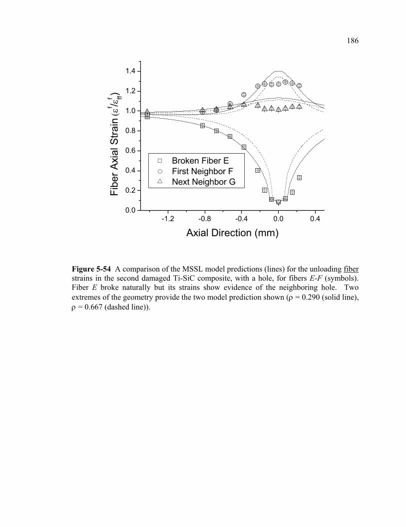
Figure 5-54 A comparison of the MSSL model predictions (lines) for the unloading fiber strains in the second damaged Ti-SiC composite, with a hole, for fibers E-F (symbols). Fiber E broke naturally but its strains show evidence of the neighboring hole. Two extremes of the geometry provide the two model prediction shown (ρ = 0.290 (solid line), ρ = 0.667 (dashed line)). .................... 186

xix Figure 5-55 A comparison of the MSSL model predictions (lines) for the unloading

matrix strains (symbols) in the Ti-SiC composite with a hole. The dashed lines depict the model predictions if the minimum distance between the fibers is used for W and the matrix thickness is used for t (ρ = 0.667). Overall the fit improves by averaging the distance between the fibers for W and reducing the thickness in the model to the average thickness of the fiber (solid line, ρ = 0.290). Matrix c is damaged near the hole contributing to the strain falling short of the model prediction. ............................................................................................................ 187

Figure 5-56 A comparison of the MSSL model predictions (lines) for the normalized unloading matrix axial strains (symbols) in the Ti-SiC composite with a hole. As above, the dashed lines depict the model predictions if the minimum distance between the fibers is used for W and the matrix thickness is used for t. Again, the overall the fit improves by averaging the distance between the fibers for W and reducing the thickness in the model to the average thickness of the fiber (solid line). Though possibly influenced by the debond in fiber G (Figure 5-54), matrix e strains fall short of the model prediction. ............................................................ 188

Figure 5-57 For completeness a final comparison of the MSSL model predictions (lines) for the unloading matrix strains (symbols) in the Ti-SiC composite with a hole. As above, the dashed line depicts the model predictions if the minimum distance between the fibers is used for W and the matrix thickness is used for t and the solid line depicts the fit for averaging the distance between the fibers W and reducing the thickness in the model to the average thickness of the fiber. The general trend depicted by the model is observed................................................. 189

Tables Table 3-1 MSSL model predictions of the axial strain concentration factors (SCFs) in

the first intact fiber at the crack plane (x = 0) for the Ti-SiC composite. .............. 64

Table 4-1 Bulk residual axial strains in the Ti-SiC composite (from Figure 4-7)........ 80

Table 4-2 Residual axial strain (10-6) evolution in damage free Ti-SiC composites averaged over all fiber and matrix regions in the beam. The first three rows correspond to measurements from the first composite examined with the point detector. The last two rows correspond to values taken from the second composite using the image plate. The second composite was also taken to a greater applied tensile stress. .......................................................................................................... 94

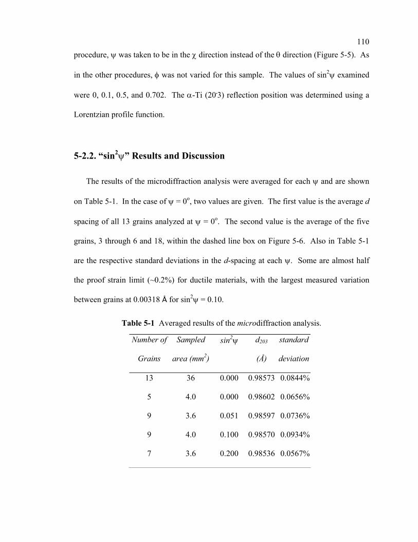
Table 5-1 Averaged results of the microdiffraction analysis...................................... 110

Table 5-3 The average axial strain in matrix regions between the fibers (lower case) and matrix regions located at the fiber (above and below, upper case). Total averages for each region are in bold. ................................................................... 136

xx

1. Introduction

1-1. Background and Motivation

Metal matrix composites (MMCs) were introduced as structural materials in the early

1970s. Nearly a decade later, with improvements in processing, applications in

aeronautics and the automotive industry began demanding materials with the specific

strength and modulus, controlled toughness and thermal expansion coefficient, hardness,

and an improved fatigue response only available from MMCs. Better understanding of

their mechanical behavior fueled improvement of the reinforcements which in turn

improved the composite properties. Consequently, MMCs have found a number of

applications which now vary from sporting goods to thermal and wear-resistant parts [1,

2].

Of the various types of MMCs (short fiber, particle, or continuous fiber reinforced),

the continuous fiber reinforced variety provides the highest structural performance.

These MMCs, usually reinforced with high modulus ceramic fibers, rely on the

continuous fibers for their strength using the matrix primarily for protection and support

of the fibers (see, for example, Figure 1-1). The matrix is also the key player for local

stress transfer between fibers. The other types of MMCs typically depend on the weaker

matrix to act also as a primary load bearing agent.

22

Figure 1-1 Some example views of continuous fiber metal matrix composites.

(a) Photograph of a two-dimensional continuous fiber metal matrix laminate composite tensile test specimen (Ti matrix/SiC fibers).

(b) Scanning electron micrograph (SEM) of the polished end of the same composite.

(c) Side view of a polished face of the laminar composite similar to that found in (a) here also using SEM.

(d) Photograph of a single fiber metal matrix composite (Al matrix/Al2O3 fiber).

(e) Fracture surface of a similar composite to (d) exposing the fiber.

(f) An SEM of the polished end of (d).

The transfer of load from a broken fiber to the rest of a composite as it is deformed is

one of the fundamental micromechanical processes determining composite strength,

lifetime and fracture toughness. It is a complex process that depends on fiber/matrix

interface properties, the constitutive behavior of matrix and fibers, the geometric

arrangement of fibers, fiber volume fraction, and fiber strength distribution. The

Fiber

Matrix

Matrix

Fiber

Fiber Matrix

Fiber Matrix

(a) (b)

(c)

(d)

(e)

(f)

23 prediction of this process is further complicated since the in situ mechanical properties of

the constituents are significantly different than the properties in the monolithic form [3, 4,

5]. These differences stem from (i) constraints imposed by neighboring phases; (ii)

changes in microstructure due to altered processing conditions required for composite

manufacturing; (iii) thermal residual stresses due to coefficient of thermal expansion

(CTE) mismatch between different phases; and in some cases, (iv) high dislocation

densities near the fiber/matrix interface [6].

Conventional stress analysis of fiber composites employs the use of strain gage

rosettes on the surface of the matrix. Test methods such as the ASTM specification

D3039-76 (1989) provide a detailed example of the traditional analysis which provides

information on the longitudinal and transverse tensile strength, Young’s moduli, tensile

strain, and major (longitudinal) and minor (transverse) Poisson’s ratios [7]. However, the

macroscopic stress-strain curves obtained by these conventional means result from the

co-deformation of the individual phases making it impossible to determine the phase-

specific in situ constitutive behavior. Typical composite deformation includes collective

nucleation and evolution of damage, fiber fractures, matrix fractures and plasticity, as

well as interface separation and sliding.

Several mechanical models have been proposed to describe the behavior of MMCs.

The simpler models such as the concentric cylinder or the Eshelby model point to the

fiber fraction as the more sensitive parameter determining a composites properties. Bulk

properties have also been predicted with relative success using finite element modeling

(FEM). Several efforts to improve computational speed over FEM have been proposed.

One of these, which uses the “shear lag” concept, will be examined in more detail in

24 Section 3-2. Reliable micromechanical models, particularly models that correctly predict

ductility in MMCs, require further development [8].

Whatever model is employed to understand an MMC, there still remains an

overwhelming need to validate or refute the predictions with relevant mechanical data.

Such data are in short supply. Modeling studies are often compared to predictions from

Monte Carlo simulations [9, 10] or incomplete subsets of data [8 (p. 241)], limiting the

ultimate relevance to the engineer who must deal with the real composite. In the Ti-SiC

composite system, micromechanical studies applying acoustic methods have been used to

identify in situ fiber breaks. But these studies do not provide the phase-specific strains in

the matrix and fibers, and only hint to the mechanism of load transfer in the composite

[11].

In order to predict the strength and lifetime of a fiber composite, the load transfer

from broken fibers to the surrounding intact material must be understood. This requires

accurate determination of stress-strain evolution at the scale of microstructure—usually

on the order of the fiber diameter. In situ measurements of stress/strain can then be used

to validate and refine predictive micromechanics models. In special cases, this has been

achieved using optical methods such as micro-Raman and piezospectroscopy [for

example: 6, 12, 13, 14, 15]. These studies provided valuable insight about fiber strains

in damaged composites at length scales approaching several µm. However, in most of

these studies either the matrix could not be characterized, or only shallow surface regions

were investigated.

More general probes that measure both the matrix strain and the reinforcement strain

are necessary to truly understand composite deformation. One such tool historically

25 useful in measuring stress is X-ray diffraction. Low-energy X-ray diffraction, on the

order of 8 keV,* has long been used to measure stress in single phase materials and,

through several technological improvements, has become a standard method for

measurements of residual stress in many materials [16, 17]. However, for most materials,

low-energy X-ray diffraction provides information specific to the material surface. This

is particularly true for MMCs where, beyond aluminum, the penetration depth of low-

energy X-rays is on the order of micrometers (e.g., 30 µm for Ti at 9 keV) and rarely

provides information on more than one layer of matrix grains. Destructive methods such

as layer removal employed low energy X-rays for depth-resolved residual strain

measurements [18, 19], but with the exception of diffraction via neutrons, observation of

continuous fiber strains under applied stress was relegated to the abovementioned

specialized cases where the matrix was optically transparent.

Neutron diffraction also remains a valuable tool in the investigation of MMC

mechanical behavior. In-depth studies of the bulk composite response to applied stress

coupled with phase-specific fiber and matrix strains have provided significant insight to

the peculiar behavior of these materials [20, 21, 22, 23, 24, 25, 26, 27, 28]. Though one

of these studies [28] does provide single fiber specific strains coupled with the elastic

portion of the matrix response, the inherent advantage of the neutron’s penetrating depth

through week nuclear interactions also limits the probe’s spatial resolution. In [28] the

researchers compensate for this drawback by increasing the fiber diameter substantially

beyond the realm of a typical MMC. The result is a measurement which is applicable to

continuum mechanics models, but entirely avoids the role of fiber matrix interactions on

*Such as X rays available from a typical Cu tube.

26 the order of the microscale [29, 30]. Other more recent investigations have shown that,

for a more traditional MMC even of the same material system, the fiber matrix interface

is characterized primarily by abrupt variations in stress never considered by continuum

mechanical models [31, 32]. Thus a general lack of information concerning MMC

deformation mechanisms at the scale of the microstructure persists.

1-2. Approach It naturally follows that a study on a practical high-performance MMC would be of

significant value to the modeling and eventually engineering community. One such

composite is the Ti-matrix/SiC-fiber laminate composite (Figure 1-1 (a)-(c)). Both Ti

and SiC are well known as high-temperature structural materials [33]. Naturally, the Ti-

SiC composite itself has received considerable attention from other researchers simply

due to the performance characteristics of its constituents [8, 11, 19, 21, 23, 24, 25, 26].

However the fundamental lack of phase-specific micromechanical data remains.

The following describes the use of X-ray diffraction to determine the phase-specific

in situ load transfer and damage evolution under applied tensile stress in a Ti-SiC

composite. Synchrotron X rays were required to obtain the necessary intensity to reduce

the beam size below the fiber diameter while maintaining sufficient diffraction statistics

and strain resolution over reasonable count times. The technique described may be

tailored to glean the specific mechanical information needed and is applicable to a variety

of composites beyond the Ti-SiC system. Multiple scales from the micro (several µm) to

macro (several mm) are simultaneously available with this method. No other technique,

including neutron diffraction, could provide the spatially resolved strain resolution from

27 multiple phases so crucial to understanding mechanical behavior of metal matrix

composites.

In this thesis, the Ti matrix and SiC fiber strains were compared to predictions from a

general micromechanics model [34]. This “matrix stiffness shear lag” (MSSL) model

accounts for the linear elastic co-deformation of fiber and matrix in a wide variety of

unidirectional fiber composites containing any configuration of multiple fractures. This

is the first damage evolution study tailored for application to a micromechanics model

conducted on a continuous fiber MMC where both matrix and fibers were investigated

simultaneously at the scale of the microstructure.

28

2. Diffraction Techniques to Study Composites

The following briefly introduces the use of X-ray diffraction to measure strain. Some

issues concerning the application of stress to a diffracting body are also presented. The

final section outlines the two primary analysis methods used to measure the strains in the

Ti-SiC composite. The specifics of each experimental procedure are presented within the

respective chapters regarding the experiments.

2-1. Strain and X-Ray Diffraction

Strain measurement with “traditional” X-ray diffraction (XRD) is a well-established

technique [16, 17]. Measurements of strain using X rays were performed as early as

1925 [35]. Recent advances include the use of high-energy X rays (with more

penetrating power) and microdiffraction with sampling volumes of several µm3. Both of

these are best performed at synchrotron facilities, and a combination of which was used

for this study.

Microdiffraction experiments such as [36] by Noyan and co-workers at the National

Synchrotron Light Source (NSLS) achieved a spatial resolution of a few µm. Their

systematic investigations of the instrument improved its accuracy and identified potential

sources of error such as beam divergence and the sphere of confusion [37, 38]. They

provided a portion of the substantial groundwork establishing microdiffraction as a viable

XRD method.

The use of high-energy X rays to sample regions deep in materials has been

demonstrated by a number of pioneering studies [examples: 39, 40, 41, 42, 43]. High-

energy synchrotron XRD provides the ability to probe buried regions in materials. The

29 high intensity of synchrotron X rays also provides excellent time and spatial resolution.

The abovementioned synchrotron XRD studies employed both monochromatic [39, 41,

42], and polychromatic [40] beams with the former yielding higher strain sensitivity (10-5

vs. 10-3). They also sampled volumes as small as several hundred µm3. Although a few

studies are noted on strain distributions around fibers in composites [39, 40, 41], none are

known that investigated the in situ mechanical behavior of phases on multiple scales.

In general, direct XRD strain measurements under kinematic diffraction conditions

are limited to crystalline phases of materials which deform elastically.* Polycrystalline

bodies deform when subjected to external or internal stress. As long as the stress is

small, the deformation is reversible. This reversible deformation is elastic strain. The X-

ray strain method requires a measurement of the lattice parameters, using a least-squares

refinement of several peaks, or lattice spacings, specific to a single peak position, in the

material.

According to Bragg’s Law, λ = 2 d sin θ, diffraction peaks arise at a particular Bragg

angle, θ, determined by the lattice spacing, d, of the atoms of a lattice in a grain (or

crystallite) which is oriented for the diffraction condition at a particular wavelength, λ.

Peak shifts determined as a difference in initial and final angles ∆(2θ) are proportional to

changes in the average distance between lattice planes, ∆d [16]. It is this change in lattice

spacing which provides the diffraction elastic lattice strain in a diffracting material:

εd d0−

d0=

(2-1)

* It is possible to deduce plastic strain information using diffraction in a crystalline body or elastic strain information from an amorphous body (as a second phase), but here these are considered indirect strain measurements.

30 where d0 is the reference lattice spacing. When d0 is from a stress-free material, the

resulting strain measured includes residual strain. Measuring residual strain using

diffraction is well developed [17]. The choice of a strain-free reference and

measurements of d0 will be presented in Section 5-2.

Although the procedure is simple to describe and understand, its appropriate

application requires extreme care, especially when considering the level of accuracy

required to measure strains.* Errors can be intrinsic to the technique (and the instrument

used) or they can result from the inhomogeneous nature of materials studied. In the

general case when stress is applied to a polycrystalline material or composite, the total

strain measured with diffraction at any point includes three terms [44]:

εijtotal = εij

o + εijinter. + εij

res. (2-2)

where, εijo is the homogeneous elastic strain due to applied stress σo (if the material were

a homogeneous isotropic body), εijinter. is the interaction (or coupling) strain due to elastic

incompatibility or inhomogeneous plastic yielding, and εijres. is residual strain. Each of

these terms is an average value over the sampling volume. Since not all the grains within

that volume contribute to the diffraction pattern, effects from heterogeneity can become

critical when sampling small volumes.

The measurement of a peak position to assign lattice spacing possesses an inherent

error associated with fitting the peak. Depending on the source of the radiation and the

conditions of the optics and specimen sampled, the peak width and profile will change.

While sensitive to lattice spacing, the peak position is also sensitive to the optical and

sample geometric configuration. Each component possesses its own contribution to the *Many materials yield or fracture before the elastic strain reaches 1% (typically 0.2% to 0.5%).

31 error in the final peak position. A good review of errors in strain measurements is

presented in [17]. In summary, the best practice to minimize error in a diffraction

experiment is to maximize the exposure time, minimize inadvertent sample translation

from the center of diffraction, and use an internal standard. An internal standard may be

composed of any suitable diffracting material not expected to change its lattice spacing

over the course of the experiment. If systematic errors from sample displacement or

other minor misalignments occur, a strain-free standard will show a peak shift which may

then be used to correct for erroneous shifts in the strained sample [45]. Internal standards

also allow samples scanned between alignments to be compared, a necessary option for

reliable residual strain measurements.

Selection of an internal standard can be difficult. Consideration must be made for

overlap in the peaks from the standard with the peaks from the specimen. There may also

be problems with exposure times, as the peak intensity from a strain-free standard is

usually much greater than a strained material due to texture, grain size effects, or strain

broadening. The best standards are available from the National Institute of Standards and

Technology (NIST); however, a well-characterized powder which provides peaks that do

not appreciably overlap will generally suffice. Several common standard powders

include: Al2O3, CeO2, LaB6, NaCl, and Si.

32

2-1.1. Strain Measurements with In Situ Mechanical Loading

With X-ray diffraction’s ability to measure strain, it follows to apply the analysis to a

body under applied stress. Mechanical loading is not new to XRD. However, in spite of

the considerable number of mechanical loading experiments performed using diffraction

to measure strain, advances in optics and peripheral equipment have maintained a realm

of continuous flux and renewal on the cutting edge of modern science. One significant

new instrument planned for the Advanced Photon Source (APS) at Argonne National

Lab, HEX-CAT (High Energy X-ray Collaborative Access Team) will dedicate much of

its time to strain measurements using high energy X-ray diffraction. New instruments are

also planned at other advanced facilities relying on neutron and X-ray diffraction (JEEP

at Diamond/ISIS, ENGIN X at ISIS, VULCAN at SNS, SMARTS at LANSCE, a parallel

optics µbeam line upgrade at X-20 (NSLS), and a 3-D spatially resolved sub-µm

polychromatic beam line replacing 7.3.3 at ALS, to name a few).

The first mechanical loading experiments on unidirectional MMC composites

performed by Caltech researchers using diffraction took advantage of the custom load

frame based on an Instron hydraulic press at the Los Alamos Neutron Science Center.

Further experiments using a small custom load frame designed by I. C. Noyan (IBM)

were performed using synchrotron XRD at APS. Modifications to the Noyan load frame

and adaptation of an Scanning Electron Microscope (SEM) load frame designed by

Fullam,* have continued to improve the capability to mechanically load composites at

Caltech while performing XRD measurements (see Figure 2-1, see also Figure 4-3,

Figure 4-5, and Figure 5-14).

*Ernest Fullam Inc., 900 Albany Shaker Rd., Latham, NY 12110-1491.

33

Area Detector

Load CellLoad Cell

Incoming X-rays

Area Detector

Load CellLoad Cell

Incoming X-rays

Figure 2-1 Photograph of adapted Fullam load frame on the goniometer at the 7.3.3 microdiffraction beam line at the Advanced Light Source. In this orientation, the open face of the load frame allows X rays to reflect from the surface of the sample.

As with any mechanical loading experiment, many factors including accurate load

cells, a stiff frame, and stable strain increments are important in providing a good

experimental tool. However, a load frame intended for use with diffraction also requires

an open or transparent beam path exposing the sample to as wide a range of visibility as

possible. Shadowing the beam by the load frame or grips limits the length of potential

specimens, and since the diffracted beam averages strain over the irradiated area of the

sample, edge effects and non-uniformities in the grip region should also be avoided. The

weight of a load frame is often critical since, in general, it should be free to rotate when

mounted on a traditional goniometer. For some special cases, very large goniometers or

other robotic platforms are available to translate a massive load frame in the beam [28].

Finally, a constant stress mode as opposed to a constant strain or displacement

34 operational mode is preferred since diffraction measurements are associated with an

exposure time sometimes approaching many hours.

When a constant load cannot be maintained, it is necessary to track the load over time

and assign the appropriate load to each scan. Here “scan” refers to the measurement of

one or more peak positions from a diffraction experiment as described below. In order to

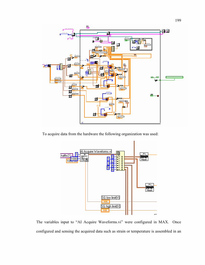
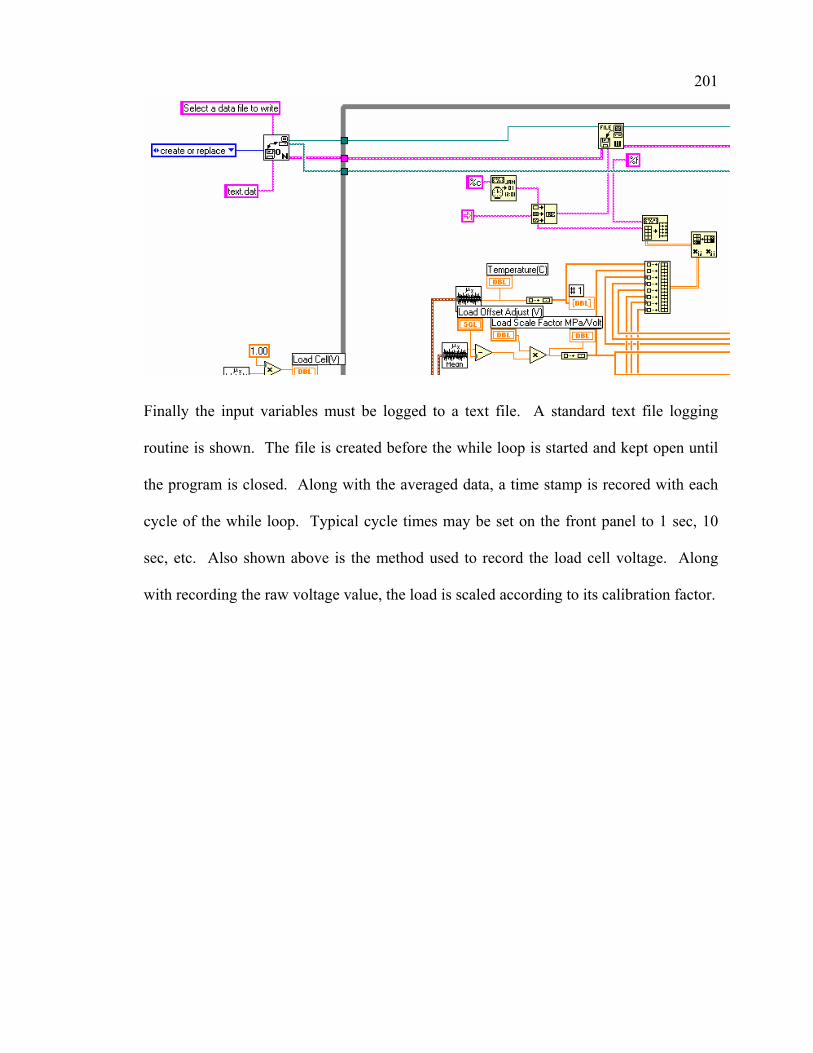
track the load on a sample mounted in an X-ray goniometer, a program was designed in

LabVIEW* 6i (see Appendix A). The load cell used was an Entran† ELHS-T1M-1KL

which requires a 10 to 15 V excitation to measure forces up to 6500 N. The output

voltage from the load cell is proportional to the applied load on the sample.

Using digitization hardware, the output voltage can be read by a computer using the

LabVIEW program. The time corresponding to the load cell reading by the computer is

correlated with the start and end time of the scan. For a typical constant displacement

experiment on metal matrix composites, the load does not change more than 0.1 MPa

during short scans. However over the course of several scans the change can become

significant enough to effect the strain measurements. Without appropriate accounting for

this change in applied stress, strain results would be misinterpreted. A secondary link,

assuring the scan times and load cell logged times are synchronized is also recommended.

When a scan starts, a digital pulse may be sent to the LabVIEW computer and logged on

the data file with the applied stress values. The pulse is particularly useful for tracking

the load during manual scans which may not be recorded at regular time intervals.

*The LabVIEW software is commercially available from National Instruments, 11500 N Mopac Expwy, Austin, TX 78759-3504. †Entran Devices, Inc. 10 Washington Ave., Fairfield, NJ 07004-3877.

35 In summary, even over the last three years, significant improvements to mechanical

loading methods coupled with diffraction strain measurements have occurred [29, 30, 31,

32]. The driving force for such improvements is difficult to define. One important factor

is the investment in advanced diffraction facilities. SMARTS is a good example of

recent improvements which were particularly clear as it stood next to a previous

generation workhorse for neutron diffraction strain measurements, NPD [28].* Similar

advances such as the high-energy beam line at APS, have reduced the constraints on the

application of mechanical load frames. Such synergistic combinations allow for high

resolution X-ray strain measurements. A methodology for these experiments is presented

in the following section.

*The Neutron Powder Diffractometer (NPD) was, as its name implies, originally dedicated to structure determination through powder diffraction. However it also, like many of its sisters, became a tool of the materials scientist.

36

2-2. High-Resolution X-Ray Strain Measurements.

High-resolution X-ray strain measurements require precise knowledge of the relative

diffracted beam position (Figure 2-2). The relative as apposed to the absolute diffracted

beam position is of interest since strain is calculated from a difference in lattice spacings,

Eq. (2-1), which would be accurate even if the absolute lattice spacings are precise but

inaccurate. For X-ray strain measurements, the overall objective is to obtain a high 2θ

spatial resolution over the range of interest. Receiving slits are a very common tool used

to improve the 2θ resolution of a diffraction measurement (Figure 2-2). Very narrow slits

potentially increase resolution but significantly reduce the signal intensity.

SlitsDiffracte

d

Beam

2θSamplePosition

TransmittedBeam

Figure 2-2 Schematic of the diffracted beam position and the position of receiving slits.

For most X-ray diffraction systems, assuming total mechanical freedom to reduce the

slit size, consideration for the available time to measure the intensity at a particular 2θ

typically fixes the lower limit of the slit width. For example, using a common Cu tube X-

ray source on a standard Siemens diffractometer, reducing the receiving slits to 0.3o from

37 3.0o will extend an hour long scan into an overnight scan with similar peak intensity.

However, with the large number of photons (or flux) available from a synchrotron X-ray

source, difficulties in manufacturing reliable narrow slits can also provide a lower

physical limit. Methods to reduce the receiving slit aperture have many forms. Slits

range from stacked plates, called Soller slits, to reduce divergence to pinhole slits with

very small apertures or with large aspect ratios maximizing the 2θ resolution at the

expense of divergence in the direction perpendicular to θ for a gain in throughput. These

slits may also be stacked to reduce divergence. A maximum angle of divergence can be

readily realized with simple geometry: for two slits a distance, S, apart, and aperture A;

the angle of maximum divergence, β, from a point source is 2 A / S. Since divergence

broadens the peak in 2θ, the strain resolution will diminish with divergent beam optics.

However, particularly with synchrotron X radiation, the source may produce a highly

parallel beam. For highly parallel optics, it is difficult and often unnecessary to

mechanically construct slits which provide a significant reduction in divergence. In

addition, parallel beam optics reduces the sensitivity to systematic errors. For parallel

optics, the most effective “slit-like” tool to improve the 2θ spatial resolution is an

analyzer crystal. Analyzer crystals consist of a single crystal which has rectangular

trough or channel cut parallel to a diffracting plane through the length of the crystal. If

properly aligned, the diffracted beam must diffract at least twice—once from each

surface of the channel—to pass through the channel in the analyzer crystal before

reaching the detector. Since it is a single crystal, the diffracted intensity is high, but only

a narrow band—a subset of an incoming divergent beam—approximately the Darwin-

Prins width [46], will diffract through the crystal for a given orientation. A peak position

38 measurement requires stepping the analyzer crystal attached to a photon counter across a

diffracted ring in 2θ at a small angular step size.* Diffraction peaks measured in this way

have a very low background and minimal detector broadening.

Fitting these peaks is typically done using a least squares technique. For synchrotron

X rays collected through an analyzer crystal, the peak profile is primarily Lorentzian. A

small Gaussian component may also be present such that a Voigt peak profile provides

the best fit. However, in some cases the statistical improvement is negligible. Several

computer programs such as PeakFit† exist for fitting typical diffraction patterns. The

peak center is determined based on a least squares fit to the peak. Errors are also

automatically calculated as a part of the peak fitting process. PeakFit reports errors as a

95% confidence limit to the peak center position which is equivalent to a 2σ level of

confidence, where σ is the standard deviation for the fit to the peak.

When fitting peaks, the diffraction pattern is input to the software. First, the

background function is subtracted. For a well-aligned synchrotron instrument, the

background is typically, over small 2θ, a linear noise function close to zero intensity.

Some detectors, such as the image plates described below, have exponential background

patterns. Samples with amorphous phases may also contribute to a particular X-ray

background. Second, the peaks are automatically or manually identified and indexed. If

more than one phase is present, multiple peak profile functions may be necessary as each

phase has its own peculiarities such as grain size that contribute to the peak shape. For

*0.005o steps were required to define some of the narrow peaks in the experiments performed at APS (Section 4-2). Compare this to a typical setting of 0.02o steps for standard measurements on a traditional Siemens D500 diffractometer.

†PeakFit© is commercially available through Jandel Scientific Software, SPSS Science, 233 S. Wacker Drive, 11th floor, Chicago, IL 60606-6307

39 example the (220) peak in the β-SiC SCS-6 fibers* is broad due to its small grain size.

Including a Gaussian component in the fit to peaks from this phase improves the certainty

in the peak center. Finally, for a strain analysis, the center of each peak is determined by

minimizing the difference between the estimated peak profile function and the diffraction

intensities. Centers reported from such a series of steps may then be immediately

converted to lattice spacings. Corrections for inadvertent translation of an internal

standard from the center of diffraction may also be performed and the resulting d is input

into Eq. 2-1.

Another option for improving the 2θ resolution requires increasing the distance

between the detector and the sample. As can be seen from Figure 2-3, when the

diffracted beam path length increases, the radius of the diffracted ring increases. Thus,

for the same ∆d, ∆(2θ) covers a longer portion of the detector. In practice, the diffracted

beam path is limited by the physical space available to the detector. For low energy

diffraction, the 2θ of interest may be large (such as 90o) and increasing the diffracted

beam path requires placing a detector in a space typically unavailable. However, at

higher energies 2θ becomes small even for high-order reflections (such as 10o) and

increasing the diffracted beam path simply requires moving the detector away from the

sample along the path of the incoming beam, z direction (Figure 2-3).

*The fibers from the composite which will be discussed in detail later (Sections 4 and 5).

40

2Θ

2Θ

x

y

zη

3/2π−η

qη 2θ,hkl

ω

φ

ψs1

s ,x3

s ,y2

z

(a) (b)

Figure 2-3 (a) Scattering geometry of a synchrotron experimental setup. x, y, z define the laboratory coordinate system, z being parallel to the incident beam, x is in the horizontal plane pointing outwards from the storage ring, and y is perpendicular to both z and x. The scattering vector q and the diffracted beam for a diffracting grain are indicated by solid arrows. Note that all scattering vectors coinciding on a cone with large opening angle (indicated by the dashed scattering vectors) are detected simultaneously on an area detector.

(b) Sample coordinate system si. The orientation of the sample coordinate system with respect to the laboratory system is shown for ω = ψ = φ = 0. (Figure adapted from [47].)

Detectors such as the digital image plate are ideal for higher-energy work. Their

maximum 2θ is limited by their diameter to a range suitable for high-energy diffraction.

They also have a small pixel size necessary for a high 2θ resolution which may be

maximized at large camera lengths (1-3 meters). The imaging plate is based on the

delayed luminescence of the alkali-earth halide BaFBr:Eu2+as a result of excitation from

X-ray irradiation. The X-ray intensity information stored in the image plate can be

recovered by optical stimulation. The mechanism of this system is described in [48].

41 Once exposed, using a Mar Digital Image Plate* 3450, a read step takes 108 seconds

to complete. It contains 1725 pixels across the radius of an image with each pixel

covering 100 x 100 µm2. From an image plate readout, scans simulating the typical 2θ

scan may be constructed by plotting the intensity given by pixels at constant η. An

example of a scan constructed in this way compared to a scan using an analyzer crystal is

shown in Figure 2-4. The scans appear comparable, but for a given energy and

alignment, the step size in 2θ may be reduced when using an analyzer crystal. In

comparison, the step size across any given peak in the digital image plate is limited by

the number of pixels on the image plate.

10 12 14 16 18 20 22 240

2000

4000

6000

8000

10000

12000

14000

Diff

ract

ed In

tens

ity (C

ount

s)

2θ (o)

SiC (220)

2400 2600 2800 3000 3200 34000

200

400

600

800

1000

1200D

iffra

cted

Inte

nsity

(Cou

nts)

Pixels (100 µm)

SiC (220)

Figure 2-4 Diffraction patterns constructed from a θ/2θ scan with an analyzer crystal at 25 keV (left) and using a strip of pixels along η = 0 from an image plate exposure at 65 keV (right). Notice the peaks are much narrower with fewer data points, marked by an “o,” in a peak using the analyzer crystal, but the image plate scan takes less than 1/8th the time and includes information from all η. (See Section 4-2 for a fully indexed pattern.)

Similar but more sensitive for digitizing X rays than film [49], the advantage of the

image plate is the additional information obtained for all η (Figure 2-3). With the image

*Commercially available from marUSA Inc., 1840 Oak Ave., Evanston, IL 60201, USA

42 plate, entire Debye-Scherrer rings are captured at multiple 2θ simultaneously. Using slits

and a point detector, the equivalent amount of information could be obtained at the

expense of a factor of 104 in data collection time [50].

The new technology requires a new method of analysis. Recently, He and Smith

published the fundamental strain equation for two-dimensional X-ray diffraction (XRD2)

[51]. They define ln(sin θ0 / sin θ) as the diffraction cone distortion at a particular (2θ,

η). Their general XRD2 equation:

f11 ε 11⋅ f12 ε 12⋅+ f22 ε 22⋅+ f13 ε 13⋅+ f23 ε 23⋅+ f33 ε 33⋅+ lnsin θ0( )sin θ( )

=

with:

f11 A2= f12 2 A⋅ B⋅= f22 B2= f13 2 A⋅ C⋅= f23 2 B⋅ C⋅= f33 C2=

a sin θ( ) cos ω( )⋅ sin η( ) cos θ( )⋅ sin ω( )⋅+=

b cos γ( )− cos θ( )=

c sin θ( ) sin ω( )⋅ sin η( ) cos θ( )⋅ cos ω( )⋅−=

A a cos φ( )⋅ b cos ψ( )⋅ sin φ( )⋅− c sin ψ( )⋅ sin φ( )⋅+=

B a sin φ( )⋅ b cos ψ( )⋅ cos φ( )⋅+ c sin ψ( )⋅ cos φ( )⋅−=

C b sin ψ( )⋅ c cos ψ( )⋅+=

provides the strain tensor for an arbitrary position of the sample and detector. For

transmission with ψ = φ = ω = 0, their strain equation reduces to

a2 ε11⋅ 2 a⋅ b⋅ ε12⋅+ b2 ε22⋅+ 2 a⋅ c⋅ ε13⋅+ 2 b⋅ c⋅ ε 23⋅+ c2 ε33⋅+ lnsin θ0( )sin θ( )

=

(2-3)

with a simplification of the coefficients to

a = sin θ

43 b = -cos η cos θ

c = -sin η cos θ

A computer program was written which is capable of performing a least squares fit of the

strain equation to the diffraction data (see Step 3 below). The software solves for the full

tensor given in (2-3). In the case of the composite studied, a two-dimensional strain state

was measured; so the calculated ε33 was averaged with the calculated ε11 giving the true

ε11 (see Appendix C for calculation details). In general, this does not have to be the case.

The advantage of the two-dimensional method used here is the reduction of error by

including the redundant information. For a biaxial strain state, the strain measured at η =

0o should also be measured at η = 180o. Furthermore the strain measured at η = 0o +/- ∆η

provides the same information as that measured at η = 180o +/- ∆η. Thus, half the

information in each exposure is not unique (assuming a continuum mechanical state*) and

serves to reduce the error in the analysis.

The analysis was developed for determining the hkl specific two-dimensional strain

tensor of multiple diffracting phases. Automation of the analysis enabled practical

implementation of spatially resolved measurements. The digital image plate can scan,

readout, and prepare for a new scan in 2 minutes. Without automation, analysis of the

same scan could take hours. Automation reduced the analysis time per scan to about 5

minutes depending on the computer power and number of phases present.

*A state in which local strain gradients must be continuous. A state that may not exist if, for example, too few grains are sampled by the beam.

44 The automated analysis, adapted from [47], consists of three main steps:

1) Convert the image plate data into a calibrated file useful for further analysis.

2) Fit the peak in 2θ at each η for all rings of interest.

3) Solve the strain tensor for each ring of interest using all peak positions from

Step 2.

The analysis program was written in MatLab* using separate MatLab code specific files

as modules for each substantial step in the analysis. Initial calibration and conversion of

the image plate files was performed using macros running on a software package called,

Fit2D†, developed by Andy Hammersley at the European Synchrotron Radiation Facility

(ESRF) [52] (see Appendix B for the necessary Fit2D macro).

Calibration of images for accurate displacement measurements is common practice

for industrial machine vision applications. Proper calibration requires imaging an object

of known dimensions using identical optics as will be used for the test measurements. An

array of objects filling the aperture at known spacing allows for nonlinear corrections or

unwarping of the entire face of the imager. In the case of strain measurements using

XRD2, a strain-free reference powder may be used to calibrate the image plate [52].

Using the same optics as will be used for the strain measurements, the diffraction rings of

the reference powder are fit to an ellipse (or series of ellipses if more than one ring is

available). Tilt misalignment may then be compensated for by digitally correcting for the

eccentricity of the standard ellipse. This eccentricity would be interpreted as deviatoric

*MatLab© is commercially available from The MathWorks, Inc., 3 Apple Hill Drive, Natick, MA 01760-2098.

†Fit2D is freely distributed software available from: http://www.esrf.fr/computing/scientific/FIT2D/index.html.

45 strain if the image is not calibrated. Fit2D provides a function for this calibration step

including built-in tools for common standard powders such as Si or CeO2.

Step 1:

Once the image plate is calibrated, the automated procedure may begin. First, the

images are converted from radial coordinates to rectangular coordinates. Performed

using Fit2D, this conversion is based on the results of the initial calibration. For

conversion, the image is cut into radially symmetric 2θ bins of constant arc length along

η. This arc length may vary from sub-degree values to a maximum integration around

the full 360o available. Smaller values improve the potential to observe deviatoric strain,

but they also increase the time required for the analysis. A larger value of arc length

serves to improve the number of grains contributing to each arc length similar to the

effect rocking along ψ would have in a more traditional experiment. The resulting

rectangular image has 2θ as its x-axis and η as its y-axis (Figure 2-5). This step provides

an opportunity to check the calibration, for if properly calibrated, in this rectangular form

rings from a phase with no deviatoric strain give a constant 2θ for all η and appear

straight in the converted image (vertical lines in Figure 2-5). All rings from the strain-

free powder should become strait in the converted image. If the strain-free powder does

not result in straight lines in the converted image, the powder is not strain-free or the

calibration of the image plate is incorrect. Once the calibration is verified, the image is

saved in Tagged Image File Format (tiff) and is ready for strain analysis.

46

Figure 2-5 The image plate, initially exposed with rings in a radial format (left), is converted to a Cartesian format (right) for analysis.

Step 2:

MatLab reads the 16 bit tiff files as a matrix with the intensity of each pixel in the tiff

file assigned a column and row position based on its pixel position in the image. After

reading the image into MatLab, a peak fitting routine is used to determine the peak center

position as a function of pixels along the x-axis (originally the 2θ direction).* This peak

fitting routine is repeated for each row of pixels. The rows are associated with a range in

η determined by the image conversion in Fit2D described above (in this analysis η was

broken up into 120 3o segments by the macro in Appendix B). The peak center, full

width at half maximum intensity (FWHM) and total integrated intensity are recorded for

*See above to Figure 2-4 for a comparison between pixels and 2θ.

2 θ

γ

γ

2 θ 2 θ

η

η

2 θ

47 each peak. Error in the peak position which improves as the inverse root of the relative

peak intensity is calculated assuming a Gaussian error distribution as standard in least

squares fitting—a built-in function of the MatLab least squares fitting routine. This

second step of the analysis is the most processor intensive and is typically repeated for all

images processed by Fit2D in the first step.

Step 3:

Lastly, the peak centers obtained in Step 2 are fit to the strain equation, Eq. (2-3) [47,

50, 51]. In Step 2 above, the fit was directly to the diffraction peak (at each η bin). Here,

in Step 3, the least square fit is to the peak centers already solved in Step 2 at all η. The

errors from the peak fits in Step 2 are propagated through to Step 3 where a total χ2 and

error in strain is calculated. The χ2 represents the sum of the difference in the fit of strain

equation to the weighted peak centers determined in Step 2. The weight of the peak

position for each azimuthal row is determined by the error for the peak at that η

diminishing the influence of low intensity regions of the ring, which becomes important

for grainy or highly textured rings. As in Step 2, the error estimation—a built in function

of MatLab—assumes a Gaussian error distribution as standard in least squares fitting.

For example, a high-intensity portion of the ring at η1 would have less error in the peak

center along 2θ for the least squares fit to that peak than a low intensity portion of the

same ring at η2 where the peak center determined by the same least squares fitting

procedure is less certain. By keeping track of these errors, the 2θ value (peak center)

from η1 has more influence than the 2θ value given by the lower intensity region at η2

making the strongest reflections have the greatest weight in the strain calculation. The

least squares fit to the strain equation, Eq. (2-3), is repeated for each ring of interest and

48 the resulting strain is tabulated in a text file for graphing and analysis of the mechanical

properties of the diffracting phases. The MatLab scripts used for this analysis are found

in Appendix C.

One drawback to this analysis is its sensitivity to outliers. A short range in 2θ is

selected for each peak of interest. This predetermined ∆(2θ) is used as a window for

fitting the peak. If the peak resides outside the window, or a second peak enters the

window, false peak positions may be recorded. This possibility limits which rings may

be considered for analysis as they must be clear of neighboring rings and have sufficient

intensity to provide a solution to the peak fitting routine. As the beam size is reduced,

variations in intensity around the ring increase. This is due to a decrease in the number of

grains diffracting for the reduced beam size. In the case of highly textured minority

phases, the intensity may be restricted to a small region in η. While a narrow acceptance

window or ∆(2θ) may eliminate the majority of outliers, a ∆(2θ) which is not a function

of η is restricted by Poison’s ratio to a value larger than otherwise necessary. In addition,

using the current method, ∆(2θ) must be large enough to accommodate the change in

radius associated with the change in strain for the phase of interest. Both of these

restrictions open up the analysis to accept potential outliers and restrict some rings from

the analysis.

Resolving these restrictions requires an iterative approach to fitting the diffraction

ring as a whole. Varying ∆(2θ) appropriately as a function of η and ε improves the

analysis method allowing the incorporation of more rings. Including more rings in the

analysis is the first step to adopting a Rietveld approach to fitting the two-dimensional

diffraction pattern. While software exists for analyzing image plate information with

49 Rietveld, these methods work best when a hydrostatic stress state is assumed for the

phases—an oversimplification for a general XRD2 strain analysis [53].

η=

0oto

360

oη

= 0o

to 3

60o

Ti (10.1) Si (220) β-Ti SiC (220) Ti (10.2)

No Shift,Strain free.

Significant Shift0.4% tensile strain

Show

s dev

iato

ricst

rain

(com

pare

to st

rain

fr

ee S

i(22

0))

Fiber Texture

Graininess

Strain broadening

η=

0oto

360

oη

= 0o

to 3

60o

Ti (10.1) Si (220) β-Ti SiC (220) Ti (10.2)

No Shift,Strain free.

Significant Shift0.4% tensile strain

Show

s dev

iato

ricst

rain

(com

pare

to st

rain

fr

ee S

i(22

0))

Fiber Texture

Graininess

Strain broadening

Figure 2-6 A zoomed-in view from two exposures of the image plate on the Ti-SiC laminar composite (see Figure 2-5 for coordinates). The first (top) is at 0 MPa applied stress, the second at 850 MPa. Axial strains appear as shifts between the two frames directly at η = 0o, 180o and 360o. Transverse strains are visible at η = 90o and 270o. For all other η the strain is a combination.

The above one- and two-dimensional analyses were used to measure the residual and

applied strains in several Ti-SiC composites. Automation of the procedure and analysis

enabled a detailed study of the micromechanics of the composite. As can be seen from

Figure 2-6, a wealth of information specific to the composite is available from the two-

dimensional analysis. Within certain limitations, the analysis may be extended to other

composites with diffracting phases. Critical issues include the three-dimensional strain

50 state, suitable grain size, X-ray penetration, a mechanism for applying stress, available

standards, and alignment of the sample plus goniometer. The expected strain state of the

Ti-SiC composite will be discussed in the next section. The grain size limitation depends

also on the beam size and will be dealt with in Section 5. Here the laminar composite

was ideal since X-ray penetration becomes less of an issue as the X-ray energy increases,

but for some other samples it is still an issue. Application of stress was dealt with above

(2-1.1), but some detriments of weak grips will be seen in Section 4-5. Available

standards and proper alignment of the sample cannot be over stated. For instance, the

residual strains reported in Section 4-4 would have been subject to an average translation

error of 60 x 10-6 strain without the use of an internal standard (Figure 2-7).

0

20

40

60

80

100

0 200 400 600

Applied Stress (MPa)

Mea

sure

d D

ispl

acem

ent E

rror

(10-6

)

x - Ti o - SiC

Figure 2-7 The translation error vs. applied load corrected for in the Ti-SiC composite. An internal Si standard powder on the composite surface provided this information.

51

3. Two-Dimensional Fiber Composite Models

This section describes two models which were used to interpret the strains measured

in the Ti-SiC composite. As will be seen in Section 4-1, the Ti-SiC laminar composite

possesses geometric, mechanical, and X-ray optical properties well suited to a

mechanical study. It is both a practical composite and a model composite allowing the

development of an analysis method which will be applicable to the study of MMCs in

general while at the same time able to reveal specific behavior of academic and industrial

value. The first model described here uses the commercially available finite element

code ABAQUS* to predict the bulk properties of the composite. The second model,

while also built on the finite element method, is based on the shear lag concept

simplifying the calculations necessary to handle the strain fields resulting from damage in

the composite.

3-1. A Finite Element Model for Ti-SiC

To better understand the bulk evolution of internal stresses/strains in the undamaged

composite, a finite element model (FEM) was developed. This model assumes plane

strain conditions because of the continuous fiber geometry. However, due to the

mechanical loading along the fiber direction, it was necessary to use a full three-

dimensional model. The plane strain assumption is then invoked by keeping the planes

perpendicular to the fiber direction (z = constant) as planes (Figure 3-1 (a)). The plane

parallel to the fiber where x is equal to half the fiber spacing is also kept planar to

produce a continuous boundary condition for an infinite number of fibers. The surface of *ABAQUS is available for an annual fee from Hibbitt, Karlsson & Sorensen, Inc., 1080 Main Street, Pawtucket, Rhode Island 02860-4847.

52 the composite (where y = t/2) is free to deform. The planes x = 0, y = 0, and z = 0 are

general symmetry planes. The relative dimensions of the fiber and matrix regions in the

model were adjusted to obtain a fiber area (and volume) fraction of 0.32 to correspond to

the measured value.

The measured thermal residual strains (see ahead to Section 4-4, Table 4-1) were

included in the calculation as they would be present in the initial state of the composite

before tensile loading. The material parameters for the matrix and the fibers were taken

from refs. [54, 55]. Specifically, the room temperature values of the elastic constants for

the matrix were Em = 125 GPa and νm = 0.31, whereas those for the fibers were

Ef = 393 GPa and νf = 0.25 (both were assumed elastically isotropic as a first order

approximation) [54]. The variation of these elastic constants with temperature was also

included in the calculation in addition to the temperature-dependent values of CTEs given

in [54]. The fibers were assumed linear elastic and intact throughout the loading. Note

that the tensile strength of the SCS-6 fibers is known to exceed 3 GPa [56]. The Ti-6Al-

4V matrix was modeled as an elastic-plastic material with a yield strength of 725 MPa

(where first deviation from linear elasticity occurs), an engineering yield strength (σ0.2) of

920 MPa and a linear strain-hardening coefficient of 1.63 GPa. These parameters were

deduced from ref. [55] where the tensile behavior of a monolithic Ti-6Al-4V alloy was

determined. A necessary starting point, since specific changes in the alloy’s material

properties as a part of the composite are unknown and hence a topic of this study.

Finally, the fiber/matrix interface was assumed intact at all times.

53

Figure 3-1 Finite element model (FEM) geometry and predictions of elastic strains at 650 MPa applied composite stress (along fiber axis, i.e., the z direction). (a) Mesh used in the FEM calculations. (b), (c) and (d) Normal strain distributions along the x, y and z directions, respectively. In (b) and (c), significant transverse strain gradients are observed across the specimen thickness. There is no variation in the longitudinal elastic strain in the fiber (d), but there is some variation in the matrix due to predicted plastic deformation around the fiber. Average longitudinal strains in the fibers due to the applied stress alone are around 3040 µε while they are about 3110 µε in the matrix. These numbers exclude the thermal residual strains and show that no significant plasticity occurs in the matrix at this applied stress.

(b) εxx

Fiber

Matrix

(c) εyy (d) εzz

(a)

54 Figure 3-1 shows the FEM geometry and the predicted elastic strains due to an

applied tensile composite stress of 650 MPa. In Figure 3-1 (b) and (c), significant

transverse strain gradients are observed across specimen thickness. As demonstrated in

ref. [57], this heterogeneity in the transverse strains makes diffraction measurements in

these directions highly dependent on positioning and prone to large errors (for example

see Section 4-5). Fortunately, there is no appreciable variation predicted in the

longitudinal elastic strain in either phase across the specimen thickness (Figure 3-1 (d)).

This minimal variation of longitudinal strain aids in the interpretation of the diffraction

strains, which represent the bulk average across the specimen thickness (Section 4).

Only a thin layer in the matrix around the fiber shows a decrease in elastic strain due

to initiation of plastic deformation. The FEM predicts the plastic deformation in the

matrix to start around 150 MPa applied composite stress. This occurs due to the three-

dimensional stress state at the interface, i.e., the matrix has longitudinal and tangential

tension and radial compression resulting in a large von Mises stress at the interface that

exceeds the uniaxial yield strength (725 MPa). Note that the contour plots in Figure 3-1

are shown in the deformed geometry. The deformations have been multiplied by a factor

of 20 for clarity. It is observed that there is a periodic variation in the thickness of the

composite as the transverse contraction in the fiber under tension is much less than that in

the matrix, rendering the estimated thickness at the positions of the fibers slightly larger

than that in between the fibers. The three-dimensinal FEM provided a context to explore

and understand the bulk properties of the composite as well as verifying the homogeneity

of axial strains required for application of through thickness averages to the predicted

55 axial strains of both models. The predictions from this FEM are compared to the

measured bulk composite strains in Section 4.

56

3-2. A Micromechanics Model for Damaged Ti-SiC

Several theoretical models have been developed to predict stress distributions in

fibers and matrix near clusters of fiber breaks in unidirectional composites. Earlier work

employed load sharing rules, such as local load sharing and global load sharing (GLS) to

approximate such stress distributions generated by fiber breaks. Simple rules allowed

analytical probability analyses of sequential fiber breaks and the prediction of strength for

small composites, see for example [58, 59, 60, 61]. In general GLS, with no stress

concentration and constant interfacial sliding, has been successfully applied to ceramic

matrix composites, see for example [62, 63]. Another class of more physically based

load-sharing models is composed of models utilizing shear lag assumptions; these

essentially model the fibers as one-dimensional structures and the matrix in-between as

deforming only in shear. Such a shear lag analysis was first applied to fiber composites

by Hedgepeth [64]. In his original work, Hedgepeth obtained analytical solutions for the

stress (or strain) concentration factors (SCFs) in intact fibers due to broken fibers in

multifiber, two-dimensional, linear elastic composites. Since then, there have been

numerous extensions of his model to consider other cases [65, 66, 67]. Considerable

simplification usually accompanies such shear lag load transfer models. Characteristic

assumptions are the tensile load is carried solely by the fibers and the load carried by a

fiber prior to fracture is transferred to the neighboring fibers by simple shear deformation

of the surrounding matrix. The Hedgepeth shear lag model is most accurate when the

fiber volume fraction, f, and the fiber/matrix modulus ratio, Ef / Em, are high, i.e.,

Ef f >> Em(1-f). This condition applies to most polymer matrix composites (PMCs), and

to some MMCs with high f values, where Ef / Em typically ranges from 4 to 6. However,

57 many composites of current interest, such as most MMCs and some PMCs with low f

values, do not fall into this category. Several recent studies using micro-Raman and

piezospectroscopic techniques have shown that as the interfiber spacing increases, the

stress concentrations in the immediate neighboring fiber decreases [6, 12, 13, 14]. Shear

lag models that do not consider longitudinal matrix stiffness have been unsuccessful in

interpreting this trend.

In Hedgepeth’s original analysis, the fibers and matrix were assumed intact and

elastic. In addition, only the longitudinal stress in the fibers and shear stress in the matrix

were predicted. Clearly, other stress components influence stress transfer, so their

incorporation would make the model more realistic and potentially capable of

interpreting experimental strain measurements. Therefore, several authors have extended

the shear lag model of Hedgepeth for matrices that sustain a portion of the applied tensile

stress [65, 66, 67]. In particular, an elastic model proposed by Fukuda and Kawata [65]

included, for the first time, effects of f on the peak stress concentration factors,

considering both the longitudinal and shear stiffness of the matrix carrying shear and

tensile stresses. Their numerical results showed that the SCF on adjacent fibers increases

with decreasing inter-fiber distance as well as with increasing elastic mismatch between

the fibers and matrix. Others have also allowed the matrix to sustain tension, usually

involving detailed three-dimensional finite element [68] or other numerical [66]

calculations on a several fiber lamina containing a small cluster of fiber breaks.

Comparing these with the original elastic shear lag model demonstrated that the

differences diminish as the number of breaks in the cluster and f increase. In virtually all

these model variations, relaxing the shear lag assumptions has led to formidable

58 analytical difficulties and a need for extensive numerical computation even for a

composite with relatively few fibers. Moreover, the dependence of the numerical

solutions on a majority of the fiber and matrix properties is not conveniently removed

through normalizations; therefore, their calculations only apply for a given set of

composite parameters.

3-2.1. Matrix Stiffness Shear-Lag (MSSL) Model

Beyerlein and Landis [34] developed the “matrix stiffness shear-lag” (MSSL) model

to quickly compute the stresses and displacements of unidirectional fiber composites in

response to multiple fiber and matrix breaks. It is intended to predict macroscopic

material properties such as toughness and lifetime. Until this work, the model had not

been applied to this composite system or tested against spatially resolved matrix strains

from a metal matrix composite.

The MSSL model assumes a planar, two-dimensional composite with a single row of

aligned, parallel and continuous fibers. The model analysis requires a finite element

model of the composite system. Figure 3-2 shows a segment of the mesh, representing a

repeating cell in the composite system which is infinite in both the transverse and axial

directions. The fibers are represented by one-dimensional axial springs and the matrix

region between any two consecutive fiber elements is represented by a pair of rectangular

finite elements. Since the transverse displacements are neglected, each element has four

degrees of freedom.

59

Figure 3-2 A representative finite element mesh from the MSSL model for a laminar fiber composite (adapted from [34]).

The index for the fiber and matrix regions is “n.” The index n for a matrix region is

adjacent to the fiber region n in the positive direction. The fiber longitudinal coordinate

is x, and the crack lies along the x = 0 plane, centered at x = 0 and n = 0. The analysis

assumes the thickness, t, in the out-of-plane direction is the same for the fibers and

matrix. The width of each matrix column is W, and the width of the fibers is D. The

transverse displacements of the system and the shear deformation of the fibers are

neglected. Both the fiber and matrix are assumed linear elastic and well bonded.

Therefore, the relevant material properties are the longitudinal Young's moduli of the

fibers and matrix, Ef and Em, respectively, and the longitudinal shear modulus of the

matrix, Gm. As indicated in Figure 3-3, both the fiber and matrix are subjected to a

uniform applied stress σ, and thus the same far-field strain ε. This model provides the

Two-Dimensional Rectangular Finite Elements (matrix)

n _ 1

n + 1

n

∆x

W/2

One-Dimensional Spring Elements (fiber)

60 average longitudinal strain over the nth fiber cross section, εf

n(x), and average matrix

longitudinal strain εmn(x) across the nth matrix region Wt.

Figure 3-3 Schematic of crack geometries under consideration (adapted from ref. [34]). (a) Case (i): two fibers are broken but the crack-tip matrix regions are intact. (b) Case (ii): in addition to two broken fibers, the crack-tip matrix regions are also broken. Components are numbered with index “n”.

As in all shear lag analyses, this model provides the average axial stress over the fiber

cross section and average shear stress between adjacent fiber and matrix nodes. For a full

description of the governing equations in this model the reader is referred to [34]. The

governing equations were derived from a treatment of the FEM in Figure 3-2. Solutions

for intact and broken fiber and matrix regions were also found. For particular damage

morphology (as in Figure 3-2), the influence superposition technique is used to solve the

governing equations. Once the influence functions are determined for a given set of

broken fiber and matrix sites, a solution is obtained for the proper weighting factors

corresponding to the fiber breaks and matrix breaks such that there exists zero stress at all

x, ξ

σ,ε σ,ε

Fiber n = +3

Fiber n = +2

Fiber n = -3

Fiber n = -2

Fiber n = -1

Fiber n = +1

Fiber n = 0

(a) Case (i)

W D

Fiber, Ef Matrix, Em, Gm Matrix n = -3

Matrix n = -2

Matrix n = -1

Matrix n = 0

Matrix n = +1

Matrix n = +2

(b) Case (ii)

Crack

61 broken sites. Practically the model requires a numerical code for its execution. The main

advantage of this technique is the computation time involves solving for the weighting

factors which only depend on the number of damaged elements in the lamina and

calculating the fiber and matrix displacements.

In dimensionless form the strain field solutions depend only on the longitudinal

stiffness ratio,

ff

mm

AEAE

=ρ (3-1)

In Eq. (3-1), Af is the cross sectional area of the fiber, and Am is the cross sectional area of

the matrix between two consecutive fibers. The ratio ρ can range from 0 to infinity, but it

is usually between 0 and 1 for most MMCs. For ρ = 0, the model yields the original

Hedgepeth solution [64].

The Ti-SiC composite (described in Section 4) was chosen as a model composite for

comparison of the strains in each phase predicted by this MSSL model at applied stress.

Based on the geometry of the Ti-SiC model composite, the stiffness ratio, ρ, was

interpreted and calculated several different ways. For all cases, the elastic constants

employed were Em = 125 GPa, and Ef = 393 GPa [54]. The matrix shear modulus, Gm,

was calculated, assuming elastic isotropy in the matrix, using Gm = Em / 2(1 + νm), with

the matrix Poisson’s ratio of νm = 0.31 [54].

Several conditions for ρ and the number of breaks were characterized in [34]. While

the model is intended for use with composites of the laminar variety, the definition of W

allows some freedom within a given geometry. In addition, the critical length in the out

62 of plane direction may be assumed equal to the matrix thickness but is not clearly defined

as such. Thus, for the etched Ti-SiC composite described in Section 5-1, ρ was

interpreted and calculated in three different ways:

1. ρ1: Using the full sample thickness (t = 200 µm), the minimum spacing

between fiber surfaces (W = 100 µm) and a fiber radius of 70 µm;

2. ρ2: Letting the thickness match the fiber diameter (t = 140 µm) and with the

same W and Af as in (1);

3. ρ3: Letting the fiber volume fraction equal its area fraction (f = 0.32, the

nominal value).

The resulting values for the stiffness ratio were ρ1 = 0.413, ρ2 = 0.289, and ρ3 = 0.591

(see Table 3-1). In the following analysis it is convenient to normalize the x coordinate

along the fiber axis as

ξ =xδ

, where δ =Ef AfW

Gmt (3-2)

Here, δ is the elastic characteristic shear lag decay length of the fiber stress (or strain)

from the maximum to the far-field fiber value as defined in the original Hedgepeth model

for ρ = 0 and one fiber break. When the matrix sustains axial load (ρ > 0), this

characteristic decay length becomes greater than the value predicted by Eq. (3-2). In

general, stress (or strain) decay lengths from fractures will increase beyond δ under

matrix and interface plasticity or creep or when there is more than one fiber break.

Two initial cases of crack configuration were considered (Figure 3-3). Since the

matrix is assumed to sustain longitudinal tensile forces, the MSSL model will

63 differentiate between a transverse matrix crack extending from the fiber break to the next

fiber, case (ii), versus no crack extension from the fiber break into the matrix, case (i).

For case (i) only the matrix regions between broken fibers are broken. For case (ii), in

addition to those broken in case (i), the two ‘crack-tip’ matrix regions between the last

broken fiber and first intact fiber are broken. The model assumes the matrix and fiber

fractures are infinitely sharp.

At the crack plane, ξ = 0, the maximum strain divided by the far-field strain, or Strain

Concentration Factor (SCF), of the first intact fiber provides an efficient test of the

model’s assumptions. For a given number of fiber breaks, the shape of the strain profile

and the SCF significantly differ between the two cases, (i) and (ii). For an intact matrix

at the crack tips, case (i), the SCF is 1.3 in the first intact fiber. This increases to 1.7

when the matrix is broken, case (ii). With an intact matrix, less load transfers to the fiber,

but with a broken matrix, the load formerly carried by both the broken fiber and the

broken matrix is shed to the surrounding intact fibers. The MSSL model predicts an

intact matrix at the crack tips leads to a strain profile where the maximum SCF in the first

intact fiber is slightly displaced from the crack plane (Figure 3-4 (c)). The fiber strain

profile is governed by the difference between the decay of the shear strain and the axial

displacement of the matrix. The axial displacement dominates near the crack plane

giving a slight rise in fiber stress from the crack plane (see ref. [34] for more discussion).

When more fibers are broken, the MSSL model also predicts an increase in the SCFs and

a broadening of the strain profiles. This enlarges the area affected by the damage zone.

64

Table 3-1 MSSL model predictions of the axial strain concentration factors (SCFs) in the first intact fiber at the crack plane (x = 0) for the Ti-SiC composite.

1 Broken Fiber 2 Broken Fibers Shear Lag

Decay

Length

δ [µm]

Stiffness

Ratio

ρ

Case (i)*:

Intact

Matrix

Case (ii):

Broken

Matrix

Case (i)*:

Intact

Matrix

Case (ii):

Broken

Matrix

252 0.289 1.14 (1.15) 1.42 1.32 (1.33) 1.70

301 0.413 1.12 (1.14) 1.45 1.29 (1.31) 1.74

329 0.591 1.10 (1.12) 1.39 1.26 (1.28) 1.79

For either case (i) which considers intact matrix at the crack tip or (ii) which

considers broken matrix at the crack tip, the SCF shows minimal sensitivity to changes in

ρ from 0.289 to 0.591 (see Table 3-1). The more discriminating variable is δ, the shear

lag characteristic decay length. This results from the dependence of δ on parameters

affecting ρ: Af, W and t (compare Eqs. (3-1) and (3-2)). Thus, the three available

stiffness ratios expand or contract the strain profiles in ξ.

Figure 3-4 compares model predictions of normalized* longitudinal strains εf/ε as a

function of ξ. Figure 3-4(a) illustrates typical differences in the MSSL model predictions

*The numbers in parentheses for case (i) indicate the maximum values of strain concentrations for this case which occur at x > 0 slightly away from the crack plane.

65 of these strain concentration profiles for case (i) and (ii) for ρ2 = 0.289. MSSL model

predictions corresponding to the three choices of ρ are plotted in Figure 3-4(b) for case

(ii) and two broken fibers. As can be seen from the graph, the choice of ρ affects the

gradient of the fiber strain with respect to ξ as well as the magnitude of relative strain for

a given ξ. The predicted maximum fiber strain concentrations adjacent to the break are

1.287, 1.316, and 1.258 for case (i); and 1.740, 1.703, and 1.786 for case (ii), for ρ1-3

respectively.

*A subtlety within the definition of normalized longitudinal strain lies with the practical definition of the far-field strain which is the denominator in εf/ε or εm/ε (normalized fiber or matrix longitudinal strain respectively). Ideally the far-field strain is defined as the strain of the composite an infinite axial distance from the region or (gage section) of interest. Naturally this far-field strain would be equivalent for the matrix and the fibers. However, practically the far-field strain may not be reached within a particular gage section and more likely, even if the far-field strain is asymptotically approached within the gage section, it may not be conveniently measured.

For a particular data set, it may be easily verified that the fiber and matrix strains begin approaching a similar value, but to correctly normalize the strains to the (possibly fictitious) far-field strain, the strains must actually be “normalized” with the strains measured at large ξ. This strain is not necessarily constant from matrix to fiber (or broken matrix to broken fiber) region but should be similar, if ξ is sufficiently large. To correctly account for this practical “normalization” in the comparisons between the data and model, the resulting “normalized” strain at large ξ is not set equal to one, but equal to the strain predicted for that region at the equivalent ξ for which it was “normalized” (for example 0.98 or 1.02). This results in the same value as measuring the ideal far-field strain and normalizing conventionally.

66

0

0.2

0.4

0.6

0.8

1

1.2

1.4

1.6

1.8

0.0 0.1 0.2 0.3 0.4 0.5 0.6 0.7 0.8 0.9 1.0ξ

εf /ε

MSSL 1 two i MSSL 0 two iMSSL 1 two ii MSSL 0 two iiMSSL 1 one ii MSSL 0 one iiMSSL 1 one i MSSL 0 one i

a)

67

Figure 3-4 a) Case (i), and case (ii) with ρ = 0.289 for both one and two broken fibers. b) Comparison of each predicted relative strain value for each ρ value assuming two fiber breaks and case (ii). Under case (ii) for the first intact fiber next to the break εf/ε is greatest for ρ = 0.591, while it is least for ρ = 0.289. c) Under case (i) for the first intact fiber next to the break εf/ε is greatest for ρ = 0.289, while it is least for ρ = 0.591. Case (ii) and (i) refer to strain profiles for fibers with and without failure in the matrix adjacent to the fiber break respectively.

Clearly, the fiber most sensitive to initial assumptions in the model is the first intact

fiber next to the break. Even for this fiber, the predicted difference for each value of ρ is

small compared to the differences seen in the strains for case (i) or case (ii). In the MSSL

model, unlike in typical shear lag analyses, the shear stresses and strains are not constant

from fiber surface to fiber surface since the matrix sustains longitudinal load. For

simplicity, the model divides each matrix region in half and calculates the shear strain,

ηn,n, and stress, τn,n, in the left half and right half of any matrix region n (Figure 3-2). At

a fixed x, the gradients in shear stress between fiber surfaces increase with ρ. For case

68 (i), the shear stress near the break increases significantly with ρ. For case (ii), the shear

stress along the nearest neighboring fiber increases with ρ. However, since primarily

longitudinal rather than shear strains were measured,* the predicted longitudinal strains

were used to verify the MSSL model.

Because of the MSSL model’s earlier successes for polymer matrix composite

systems with large ρ, its intended applicability to composites such as Ti-SiC with smaller

ρ values, and its ability to track damage evolution, an investigation to its validity was

warranted [34]. In addition, the advantages of the HEµXRD2 method are particularly

suited to comparisons with the MSSL model. Namely, the access to thickness-averaged,

spatially resolved, phase-specific elastic strains provided the opportunity to check the

MSSL model using a Ti-SiC composite.

*Shear strain was measured only with the image plate which was used for the second damaged composite (Section 4-2).

69

4. Bulk Deformation of Ti-SiC Composites

The following describes the experimental procedure and results obtained from a study

of the phase-specific bulk deformation properties of the Ti-SiC composite. The bulk

properties are defined as properties common to the composite as a whole. Rather than

specific to a particular region (such as a particular fiber), they are averaged over many

fibers and surrounding matrix. The phase-specific bulk properties provide insight on the

general behavior of the fiber and matrix as they co-deform. For example, such

understanding is necessary to identify to what load the matrix remains elastic or the

presence and evolution of residual strains. Each phase’s individual mechanical response

typically contrasts with its monolithic behavior revealing material characteristics peculiar

to the interactions between each phase in the composite. This sometimes complicated

behavior is best understood in the context of a suitable model such as the FEM described

in Section 3-1. The following includes such a comparison ultimately providing the

background for the micromechanical study presented in Section 5.

4-1. The Ti-SiC Composite

In general, Ti-SiC composites are intended for moderately high-temperature structural

applications and various versions of the composite have received interest in the literature

due to its thermal residual strains [54, 69, 70, 71, 72]. The selected composite system

consisted of a single row of unidirectional SiC fibers (Textron SCS-6, 140 µm in

diameter) in a Ti-6Al-4V matrix, prepared by a proprietary technique at 3M Corp. (St.

Paul, MN 55144). For the composite examined here, the fibers were uniformly spaced

70 with an average center-to-center distance of 240 µm. The fiber area fraction was 32%, in

agreement with the value provided by the manufacturer [73].

The SCS-6 fibers consist of a carbon core upon which SiC is grown through a two

stage technique similar to vapor deposition involving the chemical decomposition of a

silane-hydrogen gas mixture on a resistively heated graphite coated carbon

monofilament. The resulting grain size in the fibers is on the order of 200-300 nm in the

radial direction and 50-100 nm in the axial direction [74]. The fibers contain the cubic

phase of SiC (β-SiC) and show crystallographic texture with the (110) plane

preferentially aligned perpendicular to the axis of the fiber. The space group for β-SiC is

F -4 3 m [75]. A cross sectional view of the composite is shown in Figure 4-1. The

carbon core of the SCS-6 SiC fiber is clearly visible in this image.

71

Figure 4-1 Scanning electron microscope (SEM) image of a typical specimen cross section. The fibers are 140 µm in diameter and are almost uniformly spaced with an average center-to-center distance of 240 µm. The carbon core of the SCS-6 fibers is visible as the dark circle in the center of the fibers. Two shades of SiC are also visible in the fiber corresponding to the two stages of SiC growth in manufacturing. The final dark ring around the fiber results from a protective carbon coat applied to the finished fiber. The cracks observed in some fibers occurred during specimen preparation. The total specimen thickness is about 200 µm. The shallow grooves seen in the Ti matrix are a result of the composite processing.

The samples were sliced to a 10 mm width from a 16 mm wide strip. In order to

increase the stress at the gage section, the samples were electric discharge machined

(EDM) to a 7 mm gage width. To prevent oxidation at the surface of the sample, Al

plates were used to hold the strip. Aluminum oxidizes more easily than titanium. If not

used, a TiO2 film would form on the composite which would add noise to the diffraction

patterns and alter the residual strains at the surface of the matrix. The remaining

specimen dimensions were thickness, t = 0.20 mm, gage length, L = 26.00 mm (Figure

4-2). A 120 ohm strain gage was attached to measure the applied macroscopic strain at

the surface in the longitudinal direction, parallel to the fibers (Figure 4-2).

Ti

SiC

72

Figure 4-2 Schematic showing the composite geometry used in bulk XRD experiments. The composite thickness was 0.2 mm. Fiber positions are represented by white lines within a gray matrix (for illustration only – not to scale).

Strain Gage

W=7 mm

L = 26.00 mm

σ,ε

σ,ε

Grip

Grip

Fibers Matrix

73

4-2. X-Ray Diffraction Method

The samples were examined using 25 keV X rays (wavelength, λ = 0.496 Å) at the 1-

ID-C beam line (SRI-CAT, Sector 1), Advanced Photon Source (APS), Argonne National

Laboratory. This energy was selected to assure sufficient penetration depth. For this

composite, 25 keV X rays transmit 58% of the incident beam intensity. Assuming an

exponential decay in the transmitted beam intensity from the sample surface inward, the

midpoint of the sampling volume is 91 µm from the surface facing the incoming X-ray

beam. Therefore, these measurements were not confined to a thin surface layer but were

representative of the entire thickness of the composite (200 µm).

To obtain the desired diffraction geometry (see Section 2-2, Figure 2-3), a four-circle

goniometer was used in transmission mode (Figure 4-3). The diffraction vector was

along the fiber axis, thus the diffraction patterns provided the longitudinal (or axial) strain

in the plane of the composite. The diffraction intensity was collected with a NaI

scintillator detector equipped with a Si (111) analyzer crystal. As described in Section 2-

2, the analyzer crystal improves the ultimate strain resolution. The X-ray beam size was

defined by slits on the incident beam side. An internal standard Si powder (NIST,

Standard Reference Material 640a) was attached to the specimen surface.

74

Figure 4-3 Photograph of the experimental setup used for the 25 keV measurements. The dashed line represents the transmitted and diffracted beam paths. The labels are as follows: (1) receiving slit, (2) Si diode beam stop, (3) translation stage, and (4) φ stage. θ and 2θ rotate about the y axis as shown by the curved arrow. See also Figure 2-3 b.

A nominally damage-free composite was scanned with a 2 x 2 mm2 beam to obtain

the average bulk residual strains and response of the composite to applied stress. The

θ/2θ scans were conducted over a range of 2θ = 10° to 24° (for indexed peaks, see Figure

4-4). The diffraction patterns exhibited reflections from β-SiC, α-Ti, Si powder, and to a

lesser extent β-Ti, which comprises a small fraction of the matrix. In order to allow

Rietveld refinements [76], 0.007° steps in 2θ were used. The Rietveld analysis was

performed using the GSAS package [77]. In addition, individual peaks were also fit

using a Lorentzian peak shape (peak fit method described in Section 2-2). Limited by

goniometer motor speed, the long scans required 24 minutes to complete.

x y

(2)

(1)

(3) (4)

75

10 12 14 16 18 20 22 240

2000

4000

6000

8000

10000

12000

14000D

iffra

cted

Inte

nsity

(Cou

nts)

2θ (o)

SiC (220)SiC (111)

Ti (00.2)

Ti (10.1)

Si (220)

Ti (10.2)Si (311)

Ti (11.0)

Si (400)Ti (10.3)/SiC (311)

Si (311)/Ti (10.2)

Ti (20.1)

Figure 4-4 Indexed diffraction pattern for a θ/2θ scan of the Ti/SiC composite using a 2 x 2 mm2 X-ray beam at 25 keV and a point detector.

A second undamaged composite was also illuminated with an X-ray beam of

0.5 x 0.5 mm2, but at a much higher energy, 63.5 keV (λ = 0.190 Å). A photograph of

the experimental setup is shown in Figure 4-5. The higher energy decreases the 2θ angle

of the diffraction rings allowing use of a digital image plate for recording the entire

diffraction ring as apposed to the narrow slice of the ring collected with the analyzer

crystal and scintillator detector (see Section 2-2 for the analysis procedure). The primary

advantage of the image plate for this composite is the additional diffracting grains

included for strain analysis. By including more grains, the measured average stress state

better represents the stress state of the material examined. Therefore, with the area

detector, the X-ray beam spot size can be reduced without the same loss in grain

76 representation normally seen with the point detectors [50] (an example using a

microbeam will be shown in Section 5).

Figure 4-5 Photograph of the high-energy experimental setup. The incoming and transmitted beam path is represented by the dashed line. The image plate (1) is 1111 mm from the sample. A Si diode (2) acts as a beam stop also capturing the transmitted intensity. The translation stage (3) supports the load frame in a horizontal position as opposed to the vertical position shown in Figure 4-3. An ion chamber connected to the incoming beam pipe (4) measures the intensity of the incoming beam, I0.

In accordance with the procedure described in Section 2-2, calibration of the image

plate was performed with the Fit2D software using diffracted rings from the same

standard Si powder (NIST, Standard Reference Material 640a) used also as an internal

standard (see Appendix B and [52]). The calibration simplifies the analysis by correcting

for tilt misalignment (here -0.4o) of the image plate with respect to the plane

perpendicular to the beam. The calibration can also be used to externally calibrate the

image plate, but it was not used for that purpose here.* The results of the calibration

placed the beam center at 1720.6 pixels from the left of the image and 1713.5 pixels from

* An external calibration is unimportant since the Si was also used as an internal standard and the strains derived from a difference in lattice spacings rather than absolute lattice spacings are reported (for details see discussion Section 2-2).

(1)

(4) (3)

(2)

77 the top of the image. The images were converted as “radial” scan types using 120

azimuthal (η) bins and 1700 radial (2θ) bins. The following conversion parameters were

taken from the Si calibration: a sample to detector distance of 1111 mm, a wavelength of

0.1897 Å, a rotation angle of -48.68o, detector tilt angle of -0.41o, starting azimuth (η)

angle of 0.0o, end azimuth (η) angle of 360.0o, inner radial limit of 0.0 pixels, outer radial

limit of 1700.0 pixels, and no intensity conservation was selected since the geometrical

correction and the polarization correction were used [52].

78

4-3. Mechanical Loading

Uniaxial tension was applied to each composite sample using a custom-built

aluminum load frame. A high-strength epoxy fixed brass tabs to the grip region of the

composite. Turning a ½ inch threaded nut applied load to the composite. The nut was

threaded onto a shaft connected to the sample grip with a pin. Since the grip was free to

rotate at the pin, it provided a simple method to reduce off-axis loading on the composite.

Off-axis loading promotes bending in the sample and complicates the intended stress

state of the composite.

Load was applied in constant displacement steps; therefore, the stress was not

constant with time. Upon termination of displacement, the stress decayed from a

maximum initial value. When the applied stress settled, the X-ray measurements were

performed. The settling time depends on the rigidity of the system. The observed

settling was primarily due to deformation in the grip assembly. An example constant

displacement step is shown in Figure 4-6. The composite exhibits macroscopic elastic

behavior over the strain range shown. Thus the strain drop observed by the gage is

associated with a load drop observed in the load cell.

Two loading cycles were performed on each sample analyzed for bulk strains. The

first cycle went to a lesser applied load than the second. For the first composite, the

maximum applied stress of the first cycle was 790 MPa, but the sample settled to 660

MPa for the strain measurements. The maximum applied stress of the second cycle did

not exceed 780 MPa due to failure in the grips. The grips were reinforced for the second

composite sample both to reduce the settling time between loads and increase the

maximum achievable load. The maximum applied stresses for the second composite

79 were 400 MPa and 900 MPa for the first and second cycles, respectively. XRD strain

measurements were taken in small stress intervals ranging from 10 to 30 MPa per step.

As depicted in Figure 4-6, the load intervals were not kept constant in load since the

frame was designed to maintain displacement (not load) over time. As discussed in

Section 2-1, this required constant monitoring of the load and applied strain using the

software described in Appendix A.

0

100

200

300

400

500

600

700

800

0 18 36Time (minutes)

Mic

rost

rain

Start of 2θ scan End of 2θ scan

Figure 4-6 The strain gage (small circles with a connecting line) reveals drift of strain with time associated with the relaxation of load from a typical constant displacement load step. The strain in the matrix with its associated error given by the least squares refinement is shown by the flat line. Information from the entire 2θ scan (marked by arrows) is included in the refinement. The strains given by the Ti (11.0) and Ti (10.2) is given by the “x” and the “*,” respectively. These along with the strain from the SiC (220) peak, a “o,” are shown at the position the peaks occur in time.

80

4-4. Bulk Residual Strains in the Composite

The initial bulk longitudinal* residual strains in the laminate composite are shown in

Table 4-1. Before loading, the fibers exhibit an average longitudinal compression of

–1500 µε due to thermal residual strains. The matrix balances this with an average

tensile residual strain of +2200 µε (obtained from the Rietveld analysis of the α-Ti

phase). The reference d spacings for these residual strain measurements were taken from

strain-free specimens of each phase. The systematic errors were compensated for by

subtracting the “false” strain given by the internal standard. The preparation of the

references is described along with other residual strains measurements for this composite

in Section 5-2. Based on these strains, the FEM (Section 3-1) predicts average

longitudinal stresses of –740 MPa and +350 MPa in the fibers and the matrix,

respectively.

Table 4-1 Bulk residual axial strains in the Ti-SiC composite (from Figure 4-7).

Phase β-SiC (220) α-Ti

(Rietveld) α-Ti (10·2) α-Ti (11·0)

Initial Residual Strain (x10-6)

−1530 (±70) +2200 (±150) +1670 (±20) +2890 (±20)

Employing the data for CTEs given in ref. [54], these thermal residual stress/strain

results suggest an effective stress-free temperature of 550°C. This means, during cooling

from the processing temperature, the thermal residual stresses/strains were effectively

generated starting around 550°C. One must be cautious about the accuracy of this *Here longitudinal and axial are considered synonymous since the axis of the fibers is in the longitudinal direction of the composite. This direction is also synonymous with the ε11, εxx, 1, ξ, and x directions.

81 temperature as its value depends to a large extent on the accuracy of CTE data and the

assumption of only elastic and plastic deformation in the matrix (i.e., any creep during

cooling is ignored).

The fiber strains were based on measurements from the (220) reflection of β-SiC,

which is a cubic phase. The choice to use only one reflection resulted from the high

texture and small grain size (50-100 nm [78]) found in the fibers. Few SiC reflections

were observed in the diffraction patterns, and among those, only (220) yielded good

statistics. The literature values for this system confirm the observed thermal residual

strains in the fibers. Withers and Clarke [55] and Choo et al. [69] used neutron

diffraction and quote the same residual strain value for the SiC fibers in the longitudinal

direction as was observed in this composite. The former used the (220) reflection as

well, but the latter performed Rietveld analysis on β-SiC. In addition, Rangaswamy et al.

[54] obtained a similar value (about –1300 µε) using the same reflection. In sum, the

(220) reflection of β-SiC yields representative values for the bulk strain state of the

fibers. This can also be seen in Figure 4-7 where the strains along (220) follow closely

the FEM predictions for the fibers.

The Ti-6Al-4V matrix exhibits significant elastic and plastic anisotropy. The initial

thermal residual strains are seen to vary appreciably when plane-specific strains from α-

Ti and the Rietveld “average” are compared (Table 4-1). (Note that the effect of the

minority phase in the matrix (β-Ti) in the preceding and following analyses has been

neglected due to its small percentage (less than 10 vol.%) [69].) Similar results were also

observed by other researchers. For instance, Choo et al. [69] obtained +2600 µε for the

average axial strain in α-Ti from Rietveld analysis. In addition, their plane-specific

82 residual strains are similar to those shown in Table 4-1. The residual thermal strain

anisotropy in α-Ti is due to anisotropy in its CTE (e.g., the CTE of the basal plane is

higher than that of the prism planes) as well as its plastic anisotropy [69]. The latter

would manifest itself in terms of variations in susceptibility to plastic deformation during

cooling to relieve thermal stresses. As a result, plane-specific residual strains would be

relaxed to varying degrees along prism planes in comparison with the basal planes.

83

4-5. Bulk Applied Strains

Application of tensile stress provided additional information about the plasticity in

the matrix. Figure 4-7 shows the evolution of elastic lattice strains in the matrix and

fibers, obtained from XRD data, during a loading/unloading cycle as well as the overall

composite behavior, obtained through the strain gage. Residual strains from Table 4-1

are also included in Figure 4-7. From the strain gage, the surface of the composite shows

linear elastic behavior up to 750 MPa applied stress (see also Figure 4-8). This is in

agreement with the material data collected at 3M Corp. [73]. The composite’s Young’s

modulus was 216 GPa, a value that compares well with the rule-of-mixtures prediction of

211 GPa and the nominal value provided by the manufacturer, 207 GPa [73].

84

0

100

200

300

400

500

600

700

800

-2000 -1000 0 1000 2000 3000 4000 5000 6000

Strain (x10-6)

App

lied

Com

posi

te S

tres

s (M

Pa)

Ti (Rietveld)Ti (10·2)Ti (11·0)Ti (FEM)SiC (220)SiC (FEM) Strain Gage

SiC TiComposite

Figure 4-7 Comparison of experimental strains from bulk with FEM predictions of applied composite stress vs. average elastic axial strains in the first undamaged Ti-SiC composite during a loading/unloading cycle. Strain gage values are shown together with lattice strains in the Ti (10·2), Ti (11·0) and SiC (220) reflections obtained from diffraction. Thermal residual strains are included (see Table 4-1). Note that due to load drifts not every stress level could yield suitable data for Rietveld refinement.

When phase-specific lattice strains were studied, additional information about the

mechanical behavior of the constituents was obtained. Single peak fits to the XRD

patterns showed that, as the composite was loaded up to 500 MPa, the fibers and matrix

co-deformed linearly (Figure 4-7). At higher stresses, the fibers began to strain more

than the matrix at the same applied stress. This is a clear signal of load transfer to the

fibers and implies yielding in the matrix. Unfortunately, time constraints during the

initial XRD runs prevented the application of many stress levels to more precisely

determine the in situ yield point of the matrix. A further complication was the load drift

85 due to deformation at the grips. This drift resulted in relaxation of applied stresses and

led to lower stress levels during diffraction measurements than those initially applied

(Figure 4-6). For example, although the composite was loaded to 780 MPa, the average

stress during diffraction data collection was 660 MPa (Figure 4-7). This means the

deviation from the linear curve in the lattice strains shown in Figure 4-7 resulted from

yielding in the matrix between 650 and 780 MPa applied composite stress.

The in situ matrix yielding is expected to commence as a thin layer around the fibers

(Figure 3-1 (d)). Since X rays sampled the entire cross section, matrix yielding is not

realized until a significant plastic layer forms. The measured strains then confirm the

FEM prediction that “global” yielding is not apparent until at least 600 MPa applied

stress (Section 3-1 and Figure 4-7). The resulting change in residual strain will be

presented with the next section in Table 4-2.

Similar behavior was seen in the second composite specimen examined with the

image plate. Since reinforced grips were used, greater stresses were achieved and the

load drift was diminished. The first cycle to 400 MPa showed primarily elastic strain.

The strains in the second cycle to higher applied stress revealed yielding in the matrix.

The attached strain gage shows slight global plasticity occurred in the composite after

750 MPa applied stress (Figure 4-8). The change in residual strain upon unloading also

confirms that local plastic deformation occurred in the matrix (Figure 4-9 and Figure

4-10).

86

600

700

800

900

2000 2200 2400 2600 2800 3000

Axial Strain (10-6)

Appl

ied

Axia

l Stre

ss (M

Pa)

Plastic DeformationFirst Observed

Figure 4-8 The macroscopic stress vs. strain in the first loading cycle of the second undamaged composite along the fiber direction according to strain gage data (symbols). Deformation in the composite was elastic up to at least 700 MPa with very little plastic deformation even after 800 MPa. A line from a linear regression fit to the elastic portion of the curve is plotted over the data points to help illuminate the slight deviation from linearity in the strains caused by plastic deformation.

An acceptable strain-free reference was not available for the image plate

measurements directly, so the measurements made using the Rietveld refinements on the

Ti strain-free reference were used for the matrix, and the Powder Diffraction File

(ICDD,* PDF# 74-2307) database values for SiC were used for the fibers. Though the

absolute residual strains will not be exact, this has no adverse effect on the accuracy of

observed changes in residual or applied strain (i.e., the residual strains are limited by the

accuracy of d0, but the relative strains (total strain minus the residual strain) will remain

*International Centre for Diffraction Data, 12 Campus Boulevard, Newtown Square, PA 19073-3273

87 accurate [79]). Since the true residual strains were not available, for comparison with the

FEM predictions, the residual strains in the second composite were assumed to equal the

predicted residual strains from the model fit to the first composite. In addition, assuming

the composites have the same residual strains is valid since the samples come from the

same stock.

From the nature of the analysis on the second composite, strain information in the

transverse direction is available simultaneously with the longitudinal direction. The

strains in the transverse direction are predicted to locally vary more than in the

longitudinal direction. This is due to the three-dimensional evolution of strains in the

composite (Section 3-1). This local strain variation produces an associated variation of

the peak center in 2θ at constant η for a range of η near 90o, the transverse direction.

In spite of this strain broadening in the transverse direction, which increases error in

the measured strains,* the bulk averaged transverse strain adds significant insight to the

behavior of the composite. As the stress increases in the composite, the strains are seen

to linearly increase in the fiber and matrix up to 500 MPa. Beyond this applied stress, the

transverse strains increase and decrease nonlinearly signaling anisotropic plastic

deformation (Figure 4-9 and Figure 4-10 (b)).

This nonlinear behavior should not be confused with the true bulk behavior of the

composite. It is an artifact of the analysis procedure. When a grain begins to deform *The analytical errors are smallest for the fiber axial strains (εf

11) and largest for the matrix shear strains (εm

12). In the fiber, the <111> texture for (220) weakened the reflection near η = 90o and 270o. The lower intensity increased the error for εf

22 and εf12.

In the matrix, graininess increases the error in average strain compared to the fiber. In addition strain broadening in the transverse direction associated with the range of strains in that direction increases the error of εm

22 and εm12 compared to εm

11 (see Figure 2-6 and error bars in Figure 4-9 and Figure 4-10).

88 plastically, its effective modulus decreases forcing neighboring grains to carry the

remaining load. Since many grains are included in the X-ray average elastic strain, some

of these neighboring “over stressed” grains contribute to the diffracted intensity

increasing the measured elastic strain. The larger grain size in the matrix limits the

number of grains contributing to each diffraction ring. Therefore, with the increased

potential for variation in strain among the matrix grains with increasing load, it is likely

that a few grains will be in a more optimal orientation for diffraction than the majority of

the remaining grains. If some of these optimally oriented grains are in a local

neighborhood that does not represent the bulk behavior of the composite, it may

significantly perturb the results of the analysis with abnormally large (or small) changes

in strain. This nonlinear effect is most pronounced in the transverse direction where the

strains naturally vary over the irritated area to a much greater degree than in the axial

direction. While this effect may encumber a modulus estimate from the transverse strains

at high stress, it does provide evidence of early yielding in the matrix not observed with

more conventional methods such as the strain gage analysis.

89

a)

0

100

200

300

400

500

600

700

800

900

-2000 -1000 0 1000 2000 3000 4000 5000 6000

Elastic Strain (10-6)

Axia

l App

lied

Stre

ss (M

Pa)

ε11

ε12

ε22

b)

0

100

200

300

400

500

600

700

800

900

-2000 -1000 0 1000 2000 3000 4000 5000 6000

Elastic Strain (10-6)

Axia

l App

lied

Stre

ss (M

Pa) ε12

ε22

ε11

Figure 4-9 Elastic bulk strains in the fiber (a) and matrix (b) for increasing applied tensile stress in the second cycle (symbols) on the second undamaged composite. As before, the stress is applied along the fiber axial direction (axis 1). The FEM prediction for the loading cycle in the composite is also shown (lines). As in Figure 4-7 there is good agreement with the model up to the higher stresses. The deviation near 800 MPa signals the onset of global plastic strain in the matrix. An early onset of plasticity is observed in the transverse (ε22) direction where individual grains naturally show larger variations in strain (see text). (Strains are taken from the matrix (10.2) diffraction ring and the fiber (220) diffraction ring.)

90

As the applied stress is increased on the composite, the matrix strains begin to change

nonlinearly in the axial direction. This deceleration in strain is associated with plastic

strain in the matrix. Since plastic strain is attributed to flow by dislocation motion and

not expansion of the lattice, the diffraction elastic strain can not continue to increase with

increasing stress. This yielding behavior is realized near 700 MPa in the axial direction,

the same stress predicted by the FEM, at least 50 MPa earlier than it is realized with the

composite strains from the gage (Figure 4-8).

One advantage of the image plate over the point detector includes improved detection

of matrix yielding. The nonlinear behavior observed in the transverse direction is more

pronounced than the axial direction. Thus matrix nonlinear behavior, which before 700

MPa was within the statistical error of the axial strains, is more significant in the

transverse strains. The nonlinear strain behavior in the transverse direction is observed as

early as 500 MPa with a significant deviation by 600 MPa. This observation is consistent

with a composite which initially yields to a small degree in the matrix along the

transverse direction near 500 MPa, yielding continues to increase spreading to an

increasing number of grains until it is initially observed in the axial direction near 700

MPa. Finally the matrix yielding becomes significant enough to affect the strain gage

reading, 250 MPa after it was first observed, near 750 MPa.

91

a)

0

100

200

300

400

500

600

700

800

900

-2000 -1000 0 1000 2000 3000 4000 5000 6000

Elastic Strain (10-6)

Axia

l App

lied

Stre

ss (M

Pa)

ε11

ε12

ε22

b)

0

100

200

300

400

500

600

700

800

900

-2000 -1000 0 1000 2000 3000 4000 5000 6000

Elastic Strain (10-6)

Axia

l App

lied

Stre

ss (M

Pa) ε12

ε22

ε11

Figure 4-10 Strains during the release of applied tensile stress in the second undamaged composite. The arrows show the direction of unloading. The fibers (a) show an overall linear behavior with very little average shear strain over the range of applied stress. However, the matrix (b) appears to deviate from linear behavior particularly in the transverse (ε22) and the shear (ε12) directions.

92 Consideration for the intrinsic range of strains in the transverse direction must be

included with these observations as the strain equation (2-3) and the analysis method was

not optimized for quantification of these variations. A broader range of strains

contributes to a more scattered position of the diffraction ring in the transverse direction

(strain broadening, for example see Figure 2-6). Since there is a greater range of strains

in this direction some grains will be closer to a yield point than others. Whereas in the

axial direction the strains are more uniform and the grains approach their yield stress

together. This becomes increasingly significant with load as XRD analysis intrinsically

weights grains unevenly which will tend to highlight grain-specific behavior particularly

in the transverse direction since only a portion of the available grains are included for

calculating the mean of the broad range. The jogs in the transverse strains of Figure 4-9

and Figure 4-10 are likely due to a small number of grains or sub-grains rotating (or

translating) slightly in and out of favorable orientation to diffraction which drastically

changes the intensity around the transverse portions of the diffracted ring for small η.

The solution to Eq. (2-3) changes for the transverse direction when these intensities

change. Again, since a broad range of strains is present in this direction, loosing intensity

for one outlier could noticeably change the result. A change which is consistent with the

onset of yielding in the matrix though the magnitude observed may not fairly represent

the mean strain in the composite.

93

4-6. Bulk Residual Strain Evolution

The outcome of matrix yielding visible in Figure 4-7, Figure 4-9, and Figure 4-10, is

quantified in Table 4-2 as the change of the residual strains following unloading.

Specifically, in the first composite—loaded to 790 MPa—new tensile strains (+300 µε)

were generated in the fibers and new compressive strains (about –200 µε using the

Rietveld analysis) were added to the matrix after unloading. The character of the

yielding-induced residual strains is typical for a MMC in which the matrix yields and

transfers load to the stiffer fibers [80, 55]. Assuming a simple one-dimensional stress

model, the change in residual strains when fully unloaded for the first composite

correspond to a 120 MPa increase in the fiber residual stress and a 25 MPa decrease in

the matrix residual stress. Compared to other loading experiments in this MMC system,

these values indicate small scale yielding in the matrix. For instance, Withers and Clarke

[55] measured residual strain changes of +1000 µε and –1800 µε in fibers and matrix,

respectively.

94 Table 4-2 Residual axial strain (10-6) evolution in damage free Ti-SiC composites averaged over all fiber and matrix regions in the beam. The first three rows correspond to measurements from the first composite examined with the point detector. The last two rows row corresponds to values taken from the second composite using the image plate. The second composite was also taken to a greater applied tensile stress.

Phase β-SiC (220)

α-Ti (Rietveld)

α-Ti (10·2)

α-Ti (11·0)

Initial Residual Strain

−1530 (±70)

+2200 (±150)

+1670 (±20)

+2890 (±20)

Final Residual Strain

−1230 (±70)

+2000 (±130)

+1400 (±20)

+2200 (±10)

1st

Composite

Change in Residual Strain After 790

MPa Applied Stress 300 (±70) -200

(±140) -270 (±20)

-690 (±15)

2nd

Composite

Change in Residual Strain After 850

MPa Applied Stress 400 (±28) NA -420

(±172) NA

Change in Residual Strain After 400

MPa Applied Stress 5 (±33) NA

-26

(±182) NA

Though a small change in the “average” matrix axial residual strains of the first

composite sample (provided by Rietveld) was observed after the plastic deformation,

significant plastic anisotropy was seen in the matrix (Figure 4-7 and Table 4-2). This is

expected given the hexagonal crystal structure of α-Ti. Of the two crystal planes

exhibited in Figure 4-7, (10·2) approaches the Rietveld average in terms of its

susceptibility to plastic deformation. Its effective elastic constant was similar to that

given by Rietveld as well—the unloading gradient of (10.2) strains was measured as 217

GPa versus 221 GPa from Rietveld. In comparison, (11.0) had an unloading gradient of

203 GPa. In addition, (10.2) is near both the (220) reflection of β-SiC and the (220)

95 reflection of Si (used as internal standard) in d spacing, reducing the data collection

times. Thus the (10.2) was also examined using the image plate analysis method. The

change in residual strain for the second composite loaded to 850 MPa is also given in

Table 4-2. The change in residual strain was in accordance with those seen in the first

composite. Furthermore, since a change in residual strain upon unloading signals

yielding in the matrix, the lack of change in residual strain for the cycle to 400 MPa

confirms the absence of matrix yielding below this stress as was concluded in the

previous section.

96

4-7. Conclusions on the Bulk Laminate Properties Using two X-ray diffraction methods, the phase-specific in situ residual and applied

strains in a metal matrix composite were investigated. Of the two methods, the use of an

image plate proved most valuable for the identification of global yielding in the matrix.

Plastic yielding is revealed in nonlinear lattice strains usually dependent on the

crystallographic direction analyzed. As was shown here, since the two-dimensional

strain tensor could be observed at each load, the characteristic nonlinear behavior of

yielding could be observed where it first occurred, the transverse direction. However,

both the point detector and the image plate methods provide elastic strains comparable to

a three-dimensional FEM (Section 3-1).

Due to the CTE mismatch, thermal residual stresses of −740 MPa in the fibers and

+350 MPa in the matrix exist along the fiber axes. Although, using conventional

mechanical testing, the global yielding of the Ti-SiC composite was not detected until

750 MPa applied stress; XRD strains revealed that measurable local yielding occurs as

early as 500 MPa. These strains were due to growth of the yield zone around the fiber as

predicted by FEM (Section 3-1). In the residual stresses and under the applied tensile

load, plastic anisotropy was observed in the matrix. It provides a source for the grain-to-

grain strain variation in the composite (Section 5).

From the applied strain results obtained here, the α-Ti (10.2) reflection shows

behavior representative of the matrix average obtained from Rietveld. The α-Ti (10.2)

also showed similar sensitivity to plasticity-induced residual strains as the matrix

average. Thus, the same reflection was used in the microdiffraction study described

below.

97

5. Microscale Deformation of Ti-SiC Composites

The bulk deformation information from the analysis above provided valuable insight

concerning the mechanical behavior of the composite. However, damage such as a fiber

break will not necessarily occur uniformly throughout the composite, making the bulk

analysis less useful in discerning the micromechanical behavior of the composite. What

is needed to fully understand the micromechanics of the composite, particularly near fiber

breaks, is spatially resolved strain information. Since damage in the composite typically

results in fiber fracture, the micromechanical dimension of interest according to the

MSSL model (Section 3-2.1) is the fiber diameter. In order to obtain strains at this scale,

XRD was used to build maps of the elastic strains near fiber breaks in the composite.

While the fibers are well suited to the micro-analysis technique, the matrix grain size is

on the order of one fifth of the fiber diameter. This presented a challenge, as only a few

grains would contribute to the measured stain at the dimensions of interest. As will be

shown, this challenge was overcome through the use of high-energy two-dimensional

micro X-ray diffraction (HEµXRD2). The observed strains are presented in this section

with a comparison to the predicted strain profiles in Section 5-7. The section begins with

the introduction of damage into the composite.

5-1. Controlled Damage in Ti-SiC Composites

In order to examine a region of interest ideal for application of the MSSL mechanics

model [34], the presence of at least one damaged fiber was required. Finding naturally

damaged fibers in situ during loading is a strong capability of X-ray imaging such as

microtopography or tomography; however, in order to isolate the effects of the damaged

98 fiber, it is also desirable to find a broken fiber that is surrounded by a uniform region of

damage free matrix and fibers. Lastly the damage must be located far from the grips and

sample edge in order to eliminate spurious effects from these regions of non-uniform

stress. Others have attempted the examination of SiC fiber strains using X-rays in a

composite processed with free fiber ends in a Ti matrix [81]. Though an interesting study

particularly for its use of radiography to identify fiber breaks, the local stress state in such

a composite does not directly relate to the problems of interest for the engineering and

modeling community since load transfer from broken to intact fibers could not be

investigated. In addition, the matrix strains between fibers were overlooked in that study.

For this analysis, two methods were used to produce controlled damage in the

continuous fiber Ti-SiC composite. In the first method, matrix at the center of the gage

length was etched (using 50% hydrofluoric acid), exposing a section of SiC fibers. In the

center of the exposed region, one fiber was damaged by compressing a sharp bit into the

fiber perpendicular to the fiber axis. The matrix was left intact around and behind the

roughly 0.6 x 0.2 mm2 exposed region or “damage area” (Figure 5-1). The fibers

examined were labeled -2 through 2 with 0 being the initially broken fiber. The specimen

dimensions were: thickness, t = 0.20 mm, gage length, L = 26.00 mm, and gage width,

W = 10.25 mm (Figure 5-2). As with the bulk composite analysis, a 120 ohm strain gage

was attached to measure the applied macroscopic strain at the surface in the longitudinal

direction, parallel to the fibers (Figure 5-2).

99

Fiber 0

Fiber +1

Fiber +2

Fiber -1

Fiber -2

510

0

95 µm

Figure 5-1 Optical micrograph illustrating the exposed fibers around the damage zone. The red numbered line is parallel to the fibers with the red numbers displaying the approximate scale for some axial positions where strains were measured.

100

Figure 5-2 Schematic showing the damaged sample geometry used in the XRD experiments. The composite thickness was 0.2 mm. Fibers positions are represented by white lines within a gray matrix. The region etched is marked by an oval below the strain gage (for illustration only – not to scale).

While the first sample afforded a good comparison with the model, uncertainty

associated with the geometry of the damage zone was alleviated by a second sample. In

the latter, a small hole was cut by plunging an EDM wire into the center of the

composite. Similar to the EDM technique first attempted on the macroscopically

analyzed sample, oxidation of the Ti surface was avoided by sandwiching the composite

between two Al strips.

Etched Region

Strain Gage

W=10.25 mm

L = 26.00 mm

σ,ε

σ,ε

Grip

Grip

Fibers Matrix

Beam Spot

101 The dimensions of the hole affect the stress concentration on the surrounding fibers.

Accurate measurement of the hole size and initially broken components is critical for

unambiguous application of micromechanical models. Using images from an SEM, the

hole measured 290 µm across cutting one fiber, labeled D, and the matrix between two

fibers, fibers D and E. The neighboring fiber, labeled E, and adjoining matrix region

were also partially cut by the EDM wire (see Figure 5-3). The length of the hole along

the fiber was measured to 240 µm. The opening of the hole in the fiber axial direction

tapers towards zero as it approaches fiber E. The average length along the cut matrix

region was measured to 226 µm.

102

CutFiber D

E

Top Surface

Cut Matrix

1

23Bottom Surface

CutFiber D

E

Top Surface

Cut Matrix

1

23Bottom Surface

Figure 5-3 An SEM image at a 45o tilt angle of the hole cut by EDM in the second composite. The hole cut completely through one fiber which was later assigned the label D. Beside it is fiber E which was partially cut. The matrix between these fibers is obviously cut as well as some of the matrix adjacent to D, the completely cut fiber.

103

5-2. Additional Residual Strain Measurements in Ti-SiC

Composites

The following describes some additional experiments focused on the residual strain in

the composite. A comparison of the results from the different techniques is presented

along with some of the difficulties in obtaining accurate residual strains from this

composite system.

For an ideal measurement of residual stress particularly in a fiber composite, a strain-

free reference is necessary. Though the chemical composition of a powder may be

identical to the consolidated phase of interest, any one of a number of processing

parameters may disturb the lattice parameter of the consolidated material making the

powder a deceptive strain-free reference. In practice, simply obtaining a strain-free

powder identical in composition to the phase of interested may also be difficult.

For the Ti-SiC composite system, a strain-free reference was obtained by etching a

portion of the matrix away from the fibers. SiC is stable in the presence of aqueous HF

and did not react with the etchant used to remove the matrix. Thus strain-free fibers, or

more precisely, fibers whose residual strain state no longer depended on the matrix were

easily attainable. Such a reference is preferred over the raw fibers since processing them

into the composite potentially changes the structure of the fibers on a scale which would

be measured by X rays (10 ppm).

A more tedious procedure of layer removal by etching was used to obtain the matrix

strain-free reference. The matrix was slowly rinsed from one surface of the composite

down to a depth exposing the radius of the fibers. As the matrix was removed, the

104 remaining composite curved away from the exposed fibers providing visual proof of the

compressive residual strain state in the fibers and tensile residual strain state in the

matrix. Finally, to completely remove the fibers from the matrix, one end of the

remaining composite was immersed in etchant. With a portion of the interface etched

away, the thermal residual stress provided enough force to separate the matrix from the

fibers resulting in the matrix strain-free reference.

Side View

Back View

Etched Side

Portion Not Etched

Figure 5-4 Two photographs of the etched composite during the process of making the strain-free reference (before the fibers were etched away from the matrix). The thermal residual strains are strikingly apparent from this image. Once the fibers were freed from the matrix both phases returned to their originally flat configuration. A razor blade is also shown to provide scale.

In some circumstances, a strain-free reference cannot be obtained. An option for

measurement of the residual strain in these cases is the “d vs. sin2ψ” technique [17]. The

technique requires measurements of the lattice spacing at one location over several

sample angular orientations (defined as ψ whether the rotation is along θ or χ). For

example, to obtain the values of sin2ψ used here (0.051, 0.10, and 0.20), the sample was

rotated in θ through the angles 13.05o, 18.43o, and 26.57o away from the θ = “2θ” / 2

105 position (or standard α = 0o position). The resulting lattice spacings are then used to

solve the relevant form of the strain equation (for example, Eq. (5-1) below) and provide

the residual strain (for more discussion see [17]).

This technique was used to measure the transverse residual strain in the matrix of the

Ti-SiC composite. Three distinct sin2ψ residual strain measurements were performed on

sections of the Ti-matrix/SiC-fiber composite consisting of a single row of unidirectional

fibers. First, a microdiffraction experiment that involved scanning the Ti matrix to

identify individual grains reflecting at a given Bragg angle for several ψ tilts is presented.

Then, two macrodiffraction experiments including a Cu radiation experiment conducted

at Caltech and a through-thickness high-energy experiment performed at the Advanced

Photon Source are compared to the microdiffraction measurements. The sampling

volume involved the same grains in both macrodiffraction cases. The analysis

illuminates the non-uniformity of residual strains in the composite, specifically in the

transverse direction, and highlights the significance in averaging data from individual

grain measurements.

106

5-2.1. “sin2ψ” Experimental Procedure

“sin2ψ” Specimen

Figure 5-5 Diagram of the low-energy microdiffraction technique. 2θ is in the same direction as θ.

For the following measurements, a separate section of unidirectional laminate from

the same Ti-SiC composite described earlier was examined. After cutting and

mechanically polishing the sample in order to expose the fibers at each surface, the

dimensions were 16 mm wide in the x* direction and 38 mm long in the y direction (see

directions in Figure 5-5). A triangular copper marker was placed near the region of

*As noted in the figure, the orientation of the x and y directions for the sin2ψ analysis are perpendicular to the directions used in the other analyses.

107 interest, which was used as the reference position for the observed grains. For this study,

the region analyzed by X rays did not have exposed fibers. Its total thickness was 0.17

mm in the z direction.

Using the linear intercept technique, the average grain size of Ti was

29 µm ± 3.5 µm [82, 83]. Measurements were made at 40x and 20x magnification on an

optical microscope. In the plane parallel to the axis of the fibers, 110 grains were

averaged (the x, y plane in Figure 5-5). For the plane perpendicular to the fibers, too few

grains were available to use the linear intercept technique.

“sin2ψ” Microdiffraction Procedure

The microdiffraction analysis was performed on the X-20 beamline of the National

Synchrotron Light Source of the Brookhaven National Laboratory using an Ω

goniometer. For this analysis, the energy of the X-rays was fixed at 9 keV providing

good statistics for count times of approximately 1 second when using a 0.2o receiving slit

width and a microbeam capillary with a 0.3o divergence in place [37]. The experiments

were conducted at room temperature.

In a reflection orientation with the fibers running perpendicular to the beam, the

sample was scanned in the plane parallel to the surface of the sample (Figure 5-5).

Individual α-Ti grains with the (20.3) plane in a similar orientation were identified by

their diffracted intensity around 2θ = 88.6o. With an X-ray spot size on the surface of the

sample approaching 10 µm in diameter, the grains were resolved as shown in Figure 5-6.

Grains were selected for further analysis based on their relative diffracted intensities.

108

Figure 5-6 Contour plot of Ti (20.3) reflection from microdiffraction. The Cu (311) reflection, which is close in d to the Ti reflection, exposes the Cu marker as the rough triangle between grains 13 and 14. The rectangle in the center of the figure borders the region scanned at higher ψ's.

The coordinates of the numbered grains shown on Figure 5-6 were optimized first in

x, then in y based on the maximum intensity of the diffracted peak while varying x and y

independently. At least two iterations of a similar optimization procedure were

performed for the θ and χ angles. Finally, 2θ was varied while holding the sample fixed.

A maximum in 2θ was then calculated based on the full width at half maximum (FWHM)

of a Gaussian curve fit to the peak. The receiving slit width for this measurement was

0.02 mm. The procedure was then repeated for sin2ψ = 0.051, 0.10, and 0.20,

respectively, on a total of 38 separate grains.

At 9 keV, the penetration depth (G0.99, defined as the thickness that contributes 99%

of the intensity diffracted in reflection at θ = 44.3o) was calculated to be 28 µm. For a

109 grain 29 µm across and a 36 mm2 area, assuming square grains, the Lorentz factor

predicts approximately 80 grains should reflect at 2θ = 88.6o [17]. As can be seen in

Figure 5-6, approximately half that number of significant grains were observed for the

36 mm2 area sampled at ψ = 0o. Thus, half of the predicted number of grains contributed

to the majority of the diffracted intensity.

“sin2ψ” Macrodiffraction Using Low Energy X Rays

The same α-Ti reflection, (20.3), was again examined at Caltech on a Siemens D500

diffractometer using Cu radiation (8.04 keV, G0.99 = 20 µm). The ψ tilts were performed

at the same angles as in the microdiffraction procedure: 0.00o, 13.00o, 18.46o, and 26.57o.

The area probed by the X-ray beam was approximately 2 mm in the x direction by 4 mm

in the y direction at 0o ψ with 0.3o slits (Figure 5-5). To correct for potential alignment

errors, a standard LaB6 powder (NIST Reference Material 660) was simultaneously

scanned in 2θ at the (411) reflection (d = 0.9798 Å). The Ti reflection was fit using a

Gaussian profile function, and the LaB6 (Kα and Kβ) reflections were fit using Lorentzian

profile functions. The d203 results are plotted on Figure 5-7.

sin2ψ Macrodiffraction Using High Energy X Rays

The same sample was again analyzed in transmission using 25 keV X-ray radiation

provided by the Advanced Photon Source (APS) at the SRI-CAT (Sector 1) beam line.

For 25 keV X-rays, G0.99 is 170 µm; therefore, the strain data obtained is a through-

thickness exponentially weighted average. An area of 2 mm along the fiber direction for

χ = 0o by 1 mm perpendicular to the fiber direction was sampled. The area investigated

intersects the area sampled by the low-energy microdiffraction sin2ψ analysis. For this

110 procedure, ψ was taken to be in the χ direction instead of the θ direction (Figure 5-5). As

in the other procedures, φ was not varied for this sample. The values of sin2ψ examined

were 0, 0.1, 0.5, and 0.702. The α-Ti (20.3) reflection position was determined using a

Lorentzian profile function.

5-2.2. “sin2ψ” Results and Discussion

The results of the microdiffraction analysis were averaged for each ψ and are shown

on Table 5-1. In the case of ψ = 0o, two values are given. The first value is the average d

spacing of all 13 grains analyzed at ψ = 0o. The second value is the average of the five

grains, 3 through 6 and 18, within the dashed line box on Figure 5-6. Also in Table 5-1

are the respective standard deviations in the d-spacing at each ψ. Some are almost half

the proof strain limit (~0.2%) for ductile materials, with the largest measured variation

between grains at 0.00318 Å for sin2ψ = 0.10.

Table 5-1 Averaged results of the microdiffraction analysis.

Number of

Grains

Sampled

area (mm2)

sin2ψ d203

(Å)

standard

deviation

13 36 0.000 0.98573 0.0844%

5 4.0 0.000 0.98602 0.0656%

9 3.6 0.051 0.98597 0.0736%

9 4.0 0.100 0.98570 0.0934%

7 3.6 0.200 0.98536 0.0567%

111 For the strain analyses calculated herein, the reference d spacing, do, value is taken as the

value measured at ψ = 0o. For φ = 0o we have [17]

dφψ

do−

doεx sin2

⋅ ψ εz cos 2ψ⋅+ εxz sin 2 ψ⋅( )⋅+

(5-1)

Using values predicted from a linear fit to the averaged values for the roughly 4 mm2

area in Table 5-1 and solving Eqn. 5-1, the relative strain in the direction perpendicular to

the fibers (εx) is −3500 µε. In the case of the microdiffraction analysis performed at ψ =

0o, the number of grains measured was significant enough to show strong variations in

the measured d spacing throughout the 36 mm2 area. These variations suggest large

strain gradients. In order to localize averaging over significant transverse strain

gradients, the sin2ψ scans were performed on an approximately 4 mm2 area of diffracting

grains (the region bordered by the dashed line box in Figure 5-6). If the d spacing given

by the entire 36 mm2 region at 0o ψ is instead used in the analysis, the result is -2400 µε.

This dependence on area exemplifies transverse strain gradients on the surface of the

polished composite sample.

The d spacing values given in Table 5-1 are plotted in Figure 5-7 along with the

values measured by the 8.04 keV macrodiffraction analysis as a function of sin2ψ. The

error bars for the microbeam analysis represent the standard deviation for the grains

averaged at that ψ. The error bars for the macrobeam analysis represent two times the

standard deviation of the (411) LaB6 reflection position measured simultaneously with

the Ti (20.3) reflection.

As can be seen from the graph, the slope of the macrodiffraction measurement agrees

with the microdiffraction measurements within the error of each measurement. Using

112 values predicted from a linear fit to the average for the macrodiffraction data and Eq. (5-

1), the predicted relative strain in the matrix is −3100 µε in the x direction (here

perpendicular to the fibers). Since, nominally, the same small number of grains was

sampled in both analyses, a similar deviation in d spacing among grains is expected. For

the macrodiffraction analysis, this deviation contributes to the broad peaks observed.

Since the low-energy experiments were performed using the θ direction for ψ, at high ψ

the spot size of the beam decreased. In addition, absorption of the diffracted radiation

becomes increasingly significant with an increase in ψ. These changes account for some

of the observed variation in intensity of the reflections with ψ.

0.9840

0.9845

0.9850

0.9855

0.9860

0.9865

0.9870

0.00 0.05 0.10 0.15 0.20sin2 (ψ)

d

Figure 5-7 Comparison of the macrobeam, , and microbeam, x, low-energy measurements.

The 25 keV data shows the matrix in transverse compression with εxx = -860 µε. The

high-energy transmission data also gives a negative slope (Table 5-2). In all three cases,

similar areas of the sample were analyzed. However, as the 25 keV results originate from

113 transmission measurements, the entire depth of the sample was probed; thus, these results

represent a larger set of grains than the previous analysis in reflection geometry.

Independent Cu Kα diffraction measurements of thick electrochemically polished Ti-

6Al-4V-matrix/SiC (SCS-6)-fiber composites gave 174 µε for the matrix residual strains

in the transverse direction [54]. The difference in these results may be due to mechanical

polishing or differences in the initial processing history, but the residual strain

measurements using the strain-free standard also gave -560 µε for the same composite

system with a strong variation depending on position from the fiber (Section 5-4).

Table 5-2 Comparison of slopes and residual strain values for each technique used.

Technique Slope of the

“d vs. sin2ψ” curve

(Å)

Residual strain in the

transverse direction

(10-6)

Microdiffraction -0.00346 -3500

Macrodiffraction -0.00307 -3100

Transmission -0.00085 -860

Transmission (using a

strain-free standard)

NA Average -560

Min. -3320

Max. 1760

114

5-2.3. “sin2ψ” Conclusions

A model Ti-SiC composite was examined using three distinct X-ray techniques: low-

energy microdiffraction (9 keV synchrotron radiation), low-energy macrodiffraction (Cu

radiation), and high-energy macrodiffraction (25 keV synchrotron radiation). When

considering similar sampling areas, the microdiffraction analysis verifies the same

compressive strain state observed using the traditional macrodiffraction technique. This

is not surprising since the same grains were observed in both cases. However, though the

“d vs. sin2ψ” plot appears linear with similar slopes for the two low-energy reflection

measurements, the strain measured in high-energy transmission is considerably different.

This is also compounded with the large variation in strain between grains.

The difference in low-energy to high-energy data suggests a large strain gradient

through the depth of the sample and likely a three-dimensional strain state making

questionable the use of “d vs. sin2ψ” data for residual strain measurements in this system.

These measurements were conducted observing lattice planes in the direction parallel to

the fiber axis (transverse direction). Measurements using transmission and a true strain-

free reference later confirmed the non-uniform strain state in this direction and a

dependence on the proximity of the measurement to the fibers in the out-of-plane

direction as is predicted by an FEM model (Sections 3-1, 4-4, and 5-4).

115

5-3. Microbeam Diffraction Method The high intensity of synchrotron X-rays makes practical the generation of small

beams that allow a detailed study of the co-deformation of phases in composites. While

the microbeam method is similar to the macrobeam method described in Section 4-2, the

addition of spatial resolution requires some procedures not covered there. A description

of these additional procedures and the resulting data follows. These microdiffraction

experiments were primarily done at the Advanced Photon Source (APS), but some

surface measurements were also performed at the National Synchrotron Light Source

(NSLS).

The composite damaged by etching (first composite) was examined with a micro X-

ray beam at 25 keV (wavelength, λ = 0.496 Å) at the 1-ID-C beam line (SRI-CAT,

Sector 1), APS. The beam size was adjusted with incoming beam slits from 30 x 30 µm2

to 90 x 90 µm2. Similar to the composite first examined with the 2 x 2 mm2 beam, the

energy was chosen to provide a through-thickness average of the strains from each phase

(see Section 4-2).

To obtain the desired diffraction geometry, a four-circle goniometer was used in

transmission mode. The diffraction vector was maintained along the fiber axis, thus the

diffraction patterns provided the longitudinal (or axial) strain in the plane of the

composite. The diffraction intensity was collected with a NaI scintillator detector

equipped with a Si (111) analyzer crystal. The X-ray beam size was defined by slits on

the incident beam side. An internal standard Si powder, (NIST, Standard Reference

Material 640a) attached to the specimen surface, verified beam and sample stability

(Figure 4-3).

116

Figure 5-8 Absorption contrast image of the damaged region in the first composite as captured by the Si diode. Intensity is proportional to absorption, i.e., the darker a region the higher the absorption. The contrast is primarily due to Ti thickness. The low density SiC fibers do not reveal features such as cracks. The absence of matrix from the surface of the sample near the damage region is evidenced by the bright region near the center of the image. The periodic change in intensity along y corresponds to the position of SiC fibers in the matrix. The fibers examined are labeled by number. Matrix regions examined lay between the labeled fibers.

The first task was to determine the location of the buried fibers around the damage

region. A Si diode, which monitored the transmitted beam intensity during each

experiment, provided contrast from X-ray absorption due to the large difference in the

absorption coefficients of the matrix and fibers: 36 cm-1 for Ti and 4.6 cm-1 for SiC (at

25 keV, from [84]). Absorption contrast maps using a 30 x 30 µm2 beam size provided

the sample coordinate system in relation to the laboratory system (Figure 5-8). At the

same time, the 2θ detector was set at fixed angles to monitor the intensity of the β-SiC

117 (220) reflection (Figure 5-9) after loading and the α-Ti (11.2) reflection (Figure 5-10)

before loading.

Figure 5-9 Map of β-SiC (220) reflection indicating the location of the buried fibers. The oval outlines the damaged region. Fibers are numbered to indicate their location with respect to the damage zone (at the beginning, “Fiber 0” was broken). It is interesting to note that the 30 x 30 µm2 beam size used in this experiment yielded a continuous map for SiC confirming its small grain size.

118

Figure 5-10 Map of α-Ti (11.2) reflection indicating the location of diffracting Ti grains. The marked damage zone and fiber locations are visible from the dashed lines available from the transmission data collected simultaneously during the scan. With an average Ti grain measuring 29 µm across, few grains are oriented for diffraction at a given θ angle. The damage zone marked by the arrow was etched to expose fibers.

At the X-20A beam line of the NSLS, similar grain maps were obtained from the α-

Ti (10.2) peak using a 10x10 µm2 beam focused by a capillary with a lower (9.1 keV)

energy. Since this reflection was used for the majority of the matrix strain measurements,

a representation of the grain distribution exposes the number and density of grains

included in the analysis. This low energy samples a depth equal to one average grain in

the matrix. For this second set of grain maps two layers of Ti grains were investigated,

first at the surface and another at the fiber midplane. These layers were available from

Damage Zone Ti Grains

Fibers

119 the surface of the matrix reference sample processed as described in Section 5-2. These

grain maps clearly show the distance between grains with respect to the scale and

position of the fibers (Figure 5-11). In keeping with the better statistics for this lattice

plane, there are more diffracting grains per area in this grain map than seen in Figure

5-10 (the difference, while apparent as shown, is even more substantial when considering

that in Figure 5-10 the entire thickness is sampled and in Figure 5-11 only the surfaces

are investigated). The grains typically have at least one to two dimensions greater than

the fiber diameter. As seen in the grain map, some elongation of the matrix grains in the

plane of the fibers was observed (likely due to processing).

120

Midplane Surface

Fiber Centers

Matrix Centers -6.55 -6.30 -6.05 -5.80 -5.55 -5.30 -5.05 -4.80 -4.55

-2.25

-2.00

-1.75

Transverse Direction (mm)

Midplane-5.50 -5.25 -5.00 -4.75 -4.50 -4.25

-3.00

-2.75

-2.50

-2.25

Counts/10kMonitor

Axia

l Dire

ctio

n (m

m)

50

200

350

500

650

800

9501000Surface

Artifact

Figure 5-11 The position of diffracting α-Ti grains that contribute to the intensity of the (10.2) reflection using a 10 x 10 µm2 X-ray beam. Since 9.1 keV X-rays are used, the examined grains are restricted to the surface of the sample. Both sides of the Ti matrix reference specimen were examined so that a layer of grains is exposed at the surface and the midplane of the sample (see Section 5-2 for description of the matrix reference). A photograph of the midplane surface is shown to the left of the contour plot. The layer at the midplane is also marked with what were fiber centers (between the black dashed lines marking the position the fibers were removed from) and matrix centers (between the grey dotted lines). The white horizontal lines are an artifact common to synchrotron analysis.

Taken together, the maps of diffracted intensity for the fibers and matrix clearly show

the contrast between the two regions. Strains measured in the fibers at a scale of the fiber

diameter will represent an average over many grains. This averaging makes the resulting

strains more representative of a continuum than would be observed if only a few grains

were available for diffraction. The total number of matrix grains irradiated by a

90 x 90 µm2 beam through the thickness of the composite is approximately 60 (assuming

the grains were 30 x 30 x 30 µm3 cubes). Strains taken from the matrix at a scale of the

121 fiber diameter will potentially represent only a fraction of these 60 grains.* Thus XRD

strains in the matrix at a scale of the fiber diameter will clearly be subject to perturbations

from intergranular stress.

The effect of broken fibers on the neighboring fiber and matrix regions was studied

with a 90 x 90 µm2 beam at APS (Figure 5-2). This spot size was selected to optimize

the diffraction intensity, while still maintaining a smaller size than either an individual

fiber or an interfiber matrix region. For the first damaged composite, the four nearest

fibers adjacent to the initially broken fiber (nos. = +1, +2, -1, -2), the broken fiber itself

(no. = 0), and the intervening matrix regions (i.e., five fibers and four matrix regions—

see Figure 5-1, Figure 5-2, Figure 3-3) were scanned along the fiber axes for a distance of

10 fiber diameters in each direction away from the break in 280 µm steps. Additionally,

at a significant distance from the break (1.89 mm from the center of the nearest scanned

fiber around the damage region), one control fiber and its adjacent matrix region were

scanned at each applied stress to obtain a measure of the in situ applied far-field strain in

the composite. The elastic lattice strains in the matrix and fibers were obtained by

monitoring one reflection from the dominant phases in each: (10·2) from α-Ti and (220)

from β-SiC. Results from the 2 x 2 mm2 beam analysis show the α-Ti (10·2) direction is

representative of the average in terms of its susceptibility to plastic deformation as well

as its effective elastic constant [85] (see also Section 4-7). The diffraction peaks were fit,

using the method of least squares, assuming a Lorentzian peak profile for each phase.

*6 to 10 of the 60 grains in the (10.2) direction would be sampled randomly using a point detector with a 90 x 90 µm2, 25 keV, 0.3o divergent incoming beam (based on the grain maps in Figure 5-11).

122

-1.5

-1.0

-0.5

0.0

0.5

1.0

1.5

6.5 7.0 7.5 8.0 8.5

Transeverse Direction (mm)

Fibe

r Axi

al D

irect

ion

(mm

)

Analyzed Positions

Line Centered On Axis of Fiber A

B C D E F G H I J

Hole In Composite

a b c d e f g h i

Figure 5-12 A map of the positions sampled for fiber and matrix strains using the image plate method on the second damaged Ti-SiC composite. Each of the 10 fibers was given a label “A” through “J”. Matrix positions are labeled “a” through “i.” A hole was cut in fiber D and its neighborhood using EDM and is marked with an oval. The axial positions at +/-1.43 mm provide information for the far-field strains. Time constraints prevented collecting data from each position on this map. Relevant subsets were examined at each applied stress and are shown separately.

The second damaged composite was also studied using a 90 x 90 µm2 beam at APS.

However, in this case the energy was increased to 65.3 keV, the axial step size was

reduced to 75 µm near the break, and additional fibers with neighboring matrix regions

were examined. The far-field strains were monitored at each matrix column or fiber at a

point 10 fiber diameters from the crack plane (Figure 5-12). In addition, to provide better

grain averaging for the matrix regions, the image plate was used in this second

123 examination. Over the course of the study 10 fibers were examined, fibers A through J.

The EDM hole cut in fiber D is visible from the radiograph in Figure 5-13.

A B C D E F G H I J-8-7-6-5-4-3-2-1012345678

Fiber Label

Fibe

r Axi

al P

ositi

on

0.920

0.929

0.938

0.947

0.956

0.966

0.975

0.984

0.9931.00

NormalizedTransmittedIntensity

Hole

Figure 5-13 The intensity of the transmitted 90 x 90 µm2 beam at 65.3 keV reveals the position of the fibers, grey columns, and the hole cut in the second damaged composite, a bright spot. Each of the 10 fibers is labeled on the x axis. The y axis provides the “Fiber Axial Position” which corresponds to the sampling position shown in Figure 5-12 numbered from the center of the hole outward in 75 µm steps. The first fiber, A, and neighboring matrix region were examined with a smaller 30 x 30 µm2 beam giving rise to the lower transmitted intensity before fiber B.

Again, the elastic lattice strains in the matrix and fibers were obtained by monitoring

the (10·2) from α-Ti and (220) from β-SiC. Calibration was also performed on both

samples using the Si (220) peak from the internal standard Si powder, (NIST, Standard

Reference Material 640a) attached to the specimen surface.

124

Figure 5-14 Photograph of the load frame mounted on the goniometer in hutch C downstream from 1-BM (bending magnet 1) at APS. The sample with a hole is shown in the grips. See inset (marked by blue rectangle) for a close-up of the composite. Placement of the strain gages is also visible in the image. The Si standard powder is mounted on the upstream side (back side in this image) of the sample.

The composites were stressed in tension using a custom-built load frame. The

attached strain gages (see Figure 5-2, and Figure 5-14) allowed the applied macroscopic

strain to be measured in a conventional fashion, thus providing a secondary means to

obtain the global behavior of the composite. While simultaneously recording the strain

from the gages, the applied load was logged by computer via a load cell. As with most

constant displacement experiments, the load would temporarily decay after it was

increased to a new value; hence, more time was required for the load to stabilize as

displacement was increased. The scan times logged with the applied stress and

Aluminum Load Frame Grip Grip

Translation Stage

Load Crank

Strain Gages

Incoming Beam Monitor

Ti/SiC Composite

Hole

125 macroscopic strain were matched to the diffraction scan times, and the stresses averaged

over the scan time.

The first damaged composite was stressed to three loads. The average stresses during

the fiber strain measurements were 90 MPa, 420 MPa, and 530 MPa. The second

damaged composite was stressed to 850 MPa. In order to identify the effects from

damage, both composites were first examined for spatially resolved residual strains. In

addition, the second damaged composite (with the EDM hole) was examined in an

unloaded condition (after the application of 850 MPa) in order to observe the change in

residual strains due to permanent deformation under load.

126

5-4. Microscale Residual Strains

The lattice spacing measured before applying stress to a composite serves two

purposes. The first is to provide a reference lattice spacing grid. This is subtracted from

the lattice spacing grid at applied load so that the change in lattice strain may be

observed. Using the unloaded composite strains as a reference for loaded strains is

particularly important for composites with a damage zone as the residual strains around

the damage zone are non-uniform. The second purpose is to measure the initial residual

strain in the composite. As with the bulk measurements (Section 4-4), this requires use

of a strain-free standard for the reference lattice spacing.

For the composite with an etched damage zone (the first damaged composite), the

examination of strains before loading the composite revealed the removal of the matrix

relaxed the longitudinal residual (thermal) strains in the fibers near the crack plane (see

Figure 5-15 and Figure 5-17). Figure 5-15 also depicts the array of positions examined

using the technique. The release of thermal residual strains was due to etching (compare

Figure 5-15 with the micrograph in Figure 5-1).

127

-2 -1 0 1 2

-5

-4

-3

-2

-1

0

1

2

3

4

5 X

XX

X

X

Fiber Label

Axia

l Pos

ition

(280

µm

ste

ps)

-3000

-2000

-1000

0

1000

2000

Axial ElasticStrain (10-6)

X

Figure 5-15 The elastic residual strains in the fibers and intervening matrix regions as a function of axial position and fiber number for the damage zone of the first composite. The shade of each square depends on the value of strain measured using the 90 x 90 µm2 beam at that position. Squares containing an “X” denote matrix positions where grains were not favorably oriented for diffraction. The position of the damage zone can be read from the relaxed (near 0) residual strains.

Since the point detector only observed grains which were oriented for diffraction

along constant η, the matrix residual strains could not be obtained in a continuous

manner along each matrix column (Figure 5-18); however, for some regions, near a grain

with the desired orientation, the diffracted intensity was high. This fluctuation in

intensity (see for example Figure 5-16) is the source for the variation in error bars in

Figure 5-18. (For more discussion on errors see Section 2-2.)

128

16.40 16.45 16.50 16.55 16.60 16.65 16.700

1000

2000

3000

4000

5000

6000

7000

8000

0

20

40

60

80

100

120

140

160

180

200

Diff

ract

ed In

tens

ity(C

ount

s/60

k M

onito

r)

2θ (o)

Ti (10.2) Strong Reflection

Ti (102)Weak Reflection

Figure 5-16 Example of diffracted peaks obtained from the matrix using the microbeam and a point detector. The weak reflection shown here contributed to an “X” for the cluster of 3 in the upper right corner of Figure 5-15. Its signal to noise is too low for adequate fitting. The background intensity is the same for both peaks.

129

10.0 10.5 11.0 11.5 12.0 12.5 13.0 13.5

-2500-2000-1500-1000

-500

-2500-2000-1500-1000

-500

-2500-2000-1500-1000-500

-2500-2000-1500-1000

-500

-2500-2000-1500-1000

-500

Fiber Axial Position (mm)

Fiber 2

Fiber -2

Fiber -1

Ela

stic

Axi

al S

train

(10-6

)

Fiber 0

Fiber 1

Figure 5-17 Residual fiber axial strain as a function of fiber axial position for the 5 fibers near the etched damage zone in the etched composite. Fiber 0 was broken before applying load. The change in strain for the fibers as a function of axial position is a result of matrix etched from above the fibers. The dashed line shows the strain given by the control fiber far from the damage region.

For the first damaged composite, the residual strains given by the control fiber

approach the values at each extreme axial position (far-field region) found in the fibers of

the damage region. These strains, -1500 µε in the fibers and +1400 µε in the matrix, also

130 agree with the bulk residual strains found in the undamaged composite (see Section 4-4).

In the far-field region, the residual strains observed with the microbeam are due to the

disparate CTE of the fiber and matrix along with the elastic and plastic anisotropy of the

matrix grains. In this region, local variations of 900 µε were observed in the matrix

across neighboring fibers with a maximum of 1700 µε and a minimum of 430 µε.

Influenced by variations in matrix strains, variation was also observed in the far-field

fiber strains (-2066 to -1366 µε). Though not available from the bulk measurements,

these variations would also be expected in the composite analyzed for bulk properties

(Section 4-4). As a comparison, the average value obtained with the 2 x 2 mm2 beam

lies within one standard deviation of the far-field microbeam measurements. Thus, the

composite’s residual stress state far from the damaged region is similar to the undamaged

composite.

131

-4000-3000-2000-1000

01000200030004000

10.0 10.5 11.0 11.5 12.0 12.5 13.0 13.5

-4000-3000-2000-1000

01000200030004000

10.0 10.5 11.0 11.5 12.0 12.5 13.0 13.5

Axia

l Ela

stic

Stra

in (1

0-6)

Between 1 & 2

Between -2 & -1

Axia

l Ela

stic

Stra

in (1

0-6)

Fiber Axial Direction (mm)

Between -1 & 0

Fiber Axial Direction (mm)

Between 0 & 1

Figure 5-18 Residual matrix axial strain as a function of fiber axial position for the 4 matrix regions between the 5 fibers examined in the first composite. Both the action of etching away matrix from the surface and breaking the fiber acted to create the observed residual strains. The change in error bar length is associated with the presence or absence of diffracting grains. The strains given by the control matrix region are marked by the dashed lines.

The effect of etching the matrix and breaking a fiber was clearly observed in the

microscale residual strains. Etching is primarily the source of the decrease in matrix

axial residual strains observed near the crack plane between fibers 0 and 1 and between

fibers -2 and -1 (Figure 5-18). Particularly between fibers -1 and 0, in addition to the

decrease observed from etching, a large degree of residual axial compression was

measured in the matrix strains due to the action of breaking fiber 0 (Figure 5-18). Even

far from the damage zone, the matrix residual strain was seen to vary by as much as 50%.

This variation was also reflected in the fiber strains creating locations where the residual

132 compressive stress partially relaxed. The difficulty in obtaining information from the

matrix is clear from the absence of strains or large error associated with the diffracted

intensity available from portions of the matrix.

In the second damaged composite with an EDM hole, the image plate technique was

applied in order to increase the number of matrix grains sampled at each position. Here,

10 fibers and the intervening matrix regions were examined. External calibration of the

absolute strains using the strain-free references was not available with this method.

Therefore, translation error between the references and the composite was not

compensated making the absolute residual strains potentially less accurate than the

residual strains measured in the previous composite. In order to observe the significance

of potential translation errors, a separate analysis of translation error was made on the

second composite using the unstrained internal standard Si powder. From the Si (220)

ring position, the standard deviation due to translation was 70 µε with random

fluctuations up to 114 µε. These errors are small compared to the measured strains, ~5%

of the total measured strain. Complications from overlap of the standard peaks with other

Ti reflections, make further study of the potential translation errors beyond the scope of

the analysis technique. However, a clear residual compressive or tensile state can be

deduced from the data obtained from the second composite. Since this composite was

processed along with the previous composite, the far-field residual strains were expected

to be similar. To distinguish strain results of the two composites, the 10 fibers were

given letter names for the composite with an EDM hole studied with the image plate

versus the numerical labels used in the first composite with an etched damage region.

133 The EDM hole visible in the transmission contour plot (Figure 5-19) was also clearly

visible in plots of the residual strain field around the hole in both the fiber and matrix (see

Figure 5-20, Figure 5-21, and Figure 5-22). The fiber axial strains were in residual

compression with a tendency towards less residual strain closer to the hole. Similar

results were obtained from the transverse fiber strains, except to a lesser degree of

tension.

D E F G H I JFar-Field

-10

-8

-6

-4

-2

0

2

4

6

8

10

Far-Field

//

Fiber Label

Fibe

r Axi

al P

ositi

on(7

5 µm

ste

ps)

0.943

0.953

0.964

0.974

0.985

0.9951.000

NormalizedTransmittedIntensity

//

Figure 5-19 For each fiber examined (D through J), the transmitted intensity measured by a silicon diode divided by the incident intensity measured by an ion chamber is plotted for each axial position sampled along the fiber. The fiber positions are identified by the lighter shade, more transmission, and the thicker matrix regions by the darker shade associated with less transmission. The hole appears the brightest. The axial position spacing is 0.075 mm except for the two extreme “far-field” positions, +/-12, which were an additional 0.6 mm from the previous point (Figure 5-12).

134

-1.5 -1.0 -0.5 0.0 0.5 1.0 1.5-2500-2000-1500-1000-500

0

-2500-2000-1500-1000-500

0

-2500-2000-1500-1000-500

0

-2500-2000-1500-1000-500

0

-2500-2000-1500-1000-500

0

Fiber Axial Position (mm)

Fiber H

Fiber D

Fiber ESi

C E

last

ic S

train

(10-6

)

Fiber F Far Field Region

Hole in the fiber

Fiber G

Figure 5-20 The axial residual fiber strain as a function of fiber axial position for fibers D through H. The “far-field region” marked by an oval will later be used to normalize the fiber strains to compare with a micromechanical model. Two more fibers, I and J, (not shown) were similar to H. The error bars are smaller than the data points for all but two points near the hole on fiber D. The poorer statistics available from these positions is due to less diffracting material in the beam.

135

D E F G H I J-12-10-8-6-4-202468

1012

Elastic AxialStrain (10-6)

Fiber Label

Fibe

r Axi

al P

ositi

on(7

5 µ m

ste

ps)

0

500

1000

1500

2000

2500

Hole

Figure 5-21 A contour plot of the matrix axial elastic residual strain for the regions associated with the fibers, marked by the fiber label, and between the fibers. The presence of the hole around axial position 0 diminishes the residual strains in the matrix around fibers D and E. Even at regions distant from the hole, variation is present in the matrix residual strains. Compare spatial resolution with Figure 5-15.

136 Table 5-3 The average axial strain in matrix regions between the fibers (lower case) and matrix regions located at the fiber (above and below, upper case). Total averages for each region are in bold.

Since matrix material exists not only between the fibers (Figure 4-1), but also above

and below the fibers, Ti matrix strains were available from both regions. The residual

axial strain from the latter matrix regions is on average 380 µε less than the strains

measured between the fibers (Table 5-3). The FEM does not predict a significant

variation in axial strains between these two matrix regions (see Section 3-1). However,

the transverse and out-of-plane strains are predicted to change significantly between these

two positions. The transverse strains change opposite to the direction observed axially

and would only influence the measured axial strains if the sample was significantly

misaligned in ψ (see Figure 2-3). The out-of-plane strains are in the direction of the

Position

Mean

Strain

(10-6)

Standard

Deviation

(10-6)

g 1239 259

H 968 371

h 1414 361

I 1051 286

i 1387 213

J 883 195

Between 1347 278

At Fibers 967 284

137 beam. Over the fiber, the FEM predicts compressive strains in the out-of-plane direction

(εyy in Figure 3-1), but between the fibers it predicts a gradual change from compressive

to tensile with an average close to zero. Some minor influence from these strains is

expected, since the scattering vector (q)* is a few degrees out of the plane of the

composite (θ = 0o with 2θ < 10o), but the 28% change observed between each position is

greater than would be caused by a few degrees in the q vector alignment. Furthermore,

since the out-of-plane strains are expected to average close to zero between the fibers,

they should have even less effect on the axial strain measurements between the fibers

even for a significant 2θ. Thus, there exists a measurable axial strain difference in the

two matrix neighborhoods not seen in the FEM.

As a comparison to the axial matrix strain measured in the acid-etched (first)

composite, the axial matrix strains measured in the EDM-cut (second) composite using

the image plate show no missing regions since grains diffracting in all η orientations are

included in the analysis (compare Figure 5-21 with Figure 5-15). Increasing the number

of sampled grains in this way causes a reduction in the measured local fluctuation of

strains suggesting the measured strains are close to an average value for the region

investigated. The additional grains also lead to a significant improvement in the average

specific error (see error bars Figure 5-22 compared to Figure 5-18). Thus, with the

analyzer crystal, grain-specific strains were revealed compared to the image plate where a

representative average strain over many grains even for the 90 x 90 µm2 region was

obtained. What does appear as scatter in the matrix residual strains should not be

*Direction along which the strain is measured (see Figure 2-3).

138 considered experimental error, but real variation in the matrix strains, a result of

intergranular stresses (Figure 5-21 and Figure 5-22).

-1.5 -1.0 -0.5 0.0 0.5 1.0 1.5

-1000-500

0500

10001500200025003000

-1000-500

0500

10001500200025003000

-1.5 -1.0 -0.5 0.0 0.5 1.0 1.5

-1000-500

0500

10001500200025003000

Fiber Axial Direction (mm)

Between I & J

Between D & E Between E & F

Mat

rix E

last

ic A

xial

Stra

in (1

0-6)

Between F & G Between G & H

Fiber Axial Direction (mm)

Between H & I

Figure 5-22 The axial residual matrix strain as a function of fiber axial position for the regions between fibers D through J. The effect of cutting the matrix is primarily visible in the matrix between fibers D and E. The other matrix regions show fluctuations in strain, but since they are also observed far from the hole, they were due to possible spatial variations in processing and/or intergranular stress. The image plate clearly improves the ability to observe matrix strain (compare with Figure 5-17).

Far from the hole, a more striking contrast between the two versions of matrix regions

was available from the matrix transverse strains. The matrix material between the fibers

was on average in a transverse residual compressive state, primarily due to thermal

residual stress. Whereas the matrix above and below the fibers is on average in a

transverse residual tensile state (Figure 5-24), also primarily due to thermal residual

139 stress. The difference between the strain states in these regions can be understood from a

three-dimensional perspective of the composite.

D E F G H I J-12-10

-8-6-4-202468

1012

Elastic Transverse Strain (10-6)

Fiber Label

Fibe

r Axi

al P

ositi

on(7

5 µm

)

-3500

-2900

-2300

-1700

-1100

-500

100

700

1300

19002000

Figure 5-24 Matrix transverse residual strain from the α-Ti (10.2) peak. Residual compressive strain (dark shade) was observed between the fibers and residual tensile strain (light shade) was observed in the matrix above and below the fibers (marked by the “Fiber Label” positions).

The main contribution to the residual strain component measured by diffraction for

the matrix regions above and below the fibers stems from the thermal mismatch between

the fiber and matrix along the circumference of the fiber. This mismatch contributes to a

residual tensile hoop strain in the matrix upon cooling. Between the fibers the

compressive residual strain is again a result of coefficient of thermal expansion

mismatch. However, in this region the contribution from the compressive radial

component of the matrix strain to diffraction is greater than the tensile hoop component.

140 Two line plots from the FEM predictions of the transverse thermal residual strain

illustrate the difference between the two positions in the matrix (Figure 5-23). Both lines

are perpendicular to the plane of the composite, but the first is centered in the fiber and

the second centered between the fibers. The FEM also reveals a variation in matrix strain

with depth (the out-of-plane direction). This variation contributes to the strain

broadening also observed in the transverse matrix strains.

141

a)

b)

0 20 40 60 80 100

0

1000

2000

3000

4000

Elas

tic T

rans

vers

eSt

rain

(10-6

)

Out-of-Plane DirectionDistance from midplane (µm)

Fiber Matrix

0 20 40 60 80 100-2000

-1500

-1000

-500

0

Out-of-Plane DirectionDistance from Midplane (µm)

Figure 5-24 a) The FEM prediction from Figure 3-1 with a solid and dashed arrow along the border of the plot exposing from where the solid and dashed lines for part “b)” were taken. b) Transverse thermal residual strain predicted in the composite by FEM. A center line along the fiber from the midplane of the composite to the surface shows tensile strain in the matrix (solid line). The transverse strains in the matrix centered between the fibers is compressive (dashed line).

In summary, the measured residual strains revealed the effect the CTE mismatch had

on each phase (axially compressive in the fibers, axially tensile in the matrix with a

periodic variation in the transverse matrix strain associated with the position of the

Midplane

Surface

142 fibers). Relaxation of the thermal residual strains in both phases was seen near the region

of damage in both composites. With the analyzer crystal, grain-specific strains were

revealed in the matrix compared to the image plate where a representative average strain

over many grains even for the 90 x 90 µm2 region was obtained. Even in the far-field

region, the grain-specific matrix residual strain was seen to vary by as much as 50%.

143

5-5. Microscale Load Sharing

In this section, the micromechanical behavior of the composite under tensile load is

explored. Again, both phases in each damaged composite are considered. The damage is

shown to evolve first through fiber failure then through matrix plasticity. The fiber and

matrix strains were measured at three applied loads in the first composite for the same

positions given in the residual strain section (Section 5-4). The second damaged

composite was examined at higher applied load. These results describe damage evolution

in the composite and will be compared with the MSSL model in Section 5-7.

For the individual fibers, the residual strains were subtracted from the total measured

strains when stress was applied. This is defined as the applied strain and will be

presented in the following figures. For the second composite, the applied load was

significant enough to induce global matrix yielding, so in addition to the applied strains

the total strain (residual + applied) will also be presented.

In the first damaged composite, fiber +1 broke between the first and second applied

stresses (90 MPa and 430 MPa). This evidence of damage evolution during loading is

depicted on Figure 5-25. This figure plots applied stress vs. axial fiber lattice strain at the

crack plane in each of the five fibers examined around the etched damage zone. From

Figure 5-25 the stress/strain behavior of fiber +1 is seen to resemble that of the initially

broken fiber, n = 0, above 100 MPa deviating from that of the intact fibers. This

deviation reveals that fiber +1 broke while applying stress to the composite. Figure 5-25

also shows that, for a given applied stress, the intact fibers closest to the broken fibers

carry the majority of the load given up by the broken fibers (i.e., at the same applied load

144 the strain is greatest for the intact fiber closest to the break). The behavior of fiber -2 (a

second nearest neighbor to the break) shows strains similar to the control fiber far from

the break.

0

100

200

300

400

500

600

700

-100 400 900 1400 1900 2400 2900 3400 3900 4400

Elastic Lattice Strain (x106)

Appl

ied

Stre

ss (M

Pa)

Fiber 2Fiber 1Fiber 0Fiber -1Fiber -2Control

Intact Fibers

Broken Fibers

Fiber 1 broke between these loads

Figure 5-25 Damage evolution under tensile load at the crack plane (x = 0 in Figure 5-1). Applied stress is plotted against applied axial lattice strain in the five fibers around the damage zone. At the beginning of loading, only fiber 0 was broken. When the stress/strain profiles of the intact and initially broken fiber are compared, it is obvious that fiber +1 broke between 90 MPa and 430 MPa.

Understanding the load transfer requires an examination of the strain along the fiber

and matrix as a function of axial position. For example, only the crack plane is shown in

Figure 5-25, but the strain transfer to the neighboring fibers is expected to occur along a

direction which results in an axial strain profile that is not necessarily maximum at the

crack plane [34, 81] (see Section 3-2.1 case (i)). In addition, the characteristic decay

length (δ, Section 3-2.1, Eq. (3-2)) for the broken fibers requires measurements of strain

at regular intervals along the fiber axial direction. The strains for the first nearest

145 neighbor to the naturally broken fiber as a function of axial position from the crack plane

were observed in fiber +2 (Figure 5-26). In addition, further confirming the break, strains

consistent with a broken fiber were identified in fiber +1 (Figure 5-27), the strain along

the axial direction in fiber +1, under the larger applied stresses, also resembles the strain

for the initially broken fiber, fiber 0 (Figure 5-28). The strains in the other first

neighboring fiber to the break (fiber -1) are seen in Figure 5-29. As seen from Figure

5-30, the second nearest neighbor also shows sensitivity to the broken fibers.

-1.5 -1.0 -0.5 0.0 0.5 1.0 1.50

500

1000

1500

2000

2500

3000

3500

4000

Elas

tic A

xial

Stra

in (1

0-6)

Fiber Axial Position From Break (mm)

530 MPa 420 MPa 90 MPa

Fiber +2

Figure 5-26 Applied strain in the first nearest neighbor fiber to the natural break (fiber +2, first damaged composite) for each load as a function of the axial position in the fiber. Load transfer (increase in strain compared to the far-field) from the broken fibers is realized even at the smaller load and continues to increase its magnitude and breath as the load increases.

146

-1.5 -1.0 -0.5 0.0 0.5 1.0 1.50

500

1000

1500

2000

2500

3000

3500

4000

Elas

tic A

xial

Stra

in (1

0-6)

Fiber Axial Position From Break (mm)

530 MPa 420 MPa 90 MPa

Fiber +1

Figure 5-27 Applied strain in fiber +1 which naturally broke while loading the first damaged composite. The fiber shows a clear decrease in strain at the break plane.

147

-1.5 -1.0 -0.5 0.0 0.5 1.0 1.50

500

1000

1500

2000

2500

3000

3500

4000

Elas

tic A

xial

Stra

in (1

0-6)

Fiber Axial Position From Break (mm)

530 MPa 420 MPa 90 MPa

Fiber 0

Figure 5-28 Applied strain in the initially broken fiber as a function of axial position from the break. The wider profile observed in this fiber’s strains compared to the naturally broken fiber are due to the extent of initial damage in the fiber. (Data also from the first damaged composite.)

148

-1.5 -1.0 -0.5 0.0 0.5 1.0 1.50

500

1000

1500

2000

2500

3000

3500

4000

Elas

tic A

xial

Stra

in (1

0-6)

Fiber Axial Position From Break (mm)

530 MPa 420 MPa 90 MPa

Fiber -1

Figure 5-29 Similar to fiber +2, the strains in the fiber which was a first nearest neighbor to the initially broken fiber as a function of axial position from the break are shown. The load transfer is first apparent at the smaller applied stress and increases with increasing stress. The profile looses symmetry with the break plane due to the damage profile in its neighbor (Figure 5-28). (Data also from the first damaged composite.)

149

-1.5 -1.0 -0.5 0.0 0.5 1.0 1.50

500

1000

1500

2000

2500

3000

3500

4000

Elas

tic A

xial

Stra

in (1

0-6)

Fiber Axial Position From Break (mm)

530 MPa 420 MPa 90 MPa

Fiber -2

Figure 5-30 Applied strain in the second nearest neighbor fiber to the break (fiber -2) for each applied load as a function of the axial position in the fiber. An effect from the broken fibers is realized even at the smaller load and continues to increase its magnitude and breath as the load increases. (Data also from the first damaged composite.)

Since the composite was examined at multiple loads, multiple strain maps for the

fibers and matrix are available. By selecting one load from the strains in the first

damaged composite shown in the above figures, a contour plot may be constructed

(Figure 5-31). Such a figure constitutes a strain map and shows spatially where load is

transferred in the composite. Ideally a higher resolution is desired giving a clearer

picture of the spatial gradients. The higher resolution was achieved with the image plate

experiment results shown below. However, the results from the first damaged composite

do show stress transfer (strain increases compared to the far-field) in the matrix and were

beneficial in comparison with the model (Section 5-7).

150 As was the case with the residual strains (Figure 5-18), the applied strains in the

matrix were not always available. However, it is clear from the observed increase in

matrix strains that load transferred to the matrix from the broken fibers. The results from

the matrix strain measurements are reported in Section 5-7 where they are compared to

the model.

-2 -1 0 1 2

-1.0

-0.5

0.0

0.5

1.0

Fiber Label (240 µm)

Fibe

r Axi

al P

osito

in (m

m)

500

1000

1500

2000

2500

3000

3500

4000

Axial ExlasticStrain (10-6)

Figure 5-31 Contour plot of the strains at the maximum applied stress (530 MPa) for all the fibers examined in the first damaged composite. The relative position of stress transfer from the break to the intact fibers is clear. The data here is taken from the last applied stress shown in Figure 5-26, Figure 5-27, Figure 5-28, Figure 5-29, and Figure 5-30.

For the second damaged composite, damaged with a hole by EDM (Section 5-1), the

10 fibers examined also show evidence of a fiber fracture during loading. A subset of the

positions sampled at the initially unstressed condition (Figure 5-12) were sampled at

850 MPa applied stress (Figure 5-32). The positions at each fiber label were analyzed for

151 fiber and matrix strains. The positions between the fiber labels were analyzed for matrix

strains. The strains for analyzed fibers are shown in Figure 5-33 and Figure 5-34. The

axial strains in the matrix are shown in Figure 5-35. The shear and transverse strains in

the matrix were also recorded (Figure 5-36 and Figure 5-37).

-1.5

-1.0

-0.5

0.0

0.5

1.0

1.5

2.0

6.5 7.0 7.5 8.0 8.5

...

Transverse Direction (mm)

Fibe

r Axi

al D

irect

ion

(mm

)

Analyzed Positions

Fiber Labels:A B C D E F G H I J

Hole in Composite

-8

-7-6

0

-5

...

Far Field Positions

Position Row

s Counted From

Hole

Figure 5-32 Each box represents a position analyzed with the 90 x 90 µm2 beam. The fibers A-J and neighboring matrix regions were analyzed in the configuration shown. These positions are a subset of the positions analyzed before stressing the composite (Figure 5-12). The numeric label for the positions used in the strain contour maps is shown on the right of the figure. For reference, the position of the hole cut in the composite is also shown in the figure.

152

A B C D E F G H I J-12

-11

-10

-9

-8

-7

-6

-5

-4

-3

-2

-1

0

1

2

3

Elastic AxialStrain (10-6)

Fiber Label

Fibe

r Axi

al P

ositi

ons

-1500-1100-700-3001005009001300170021002500290033003500

Hole

Load transfer to neighboring fibers

Figure 5-33 A strain map of the total elastic axial strains (residual + applied) in the fibers for the composite with a hole at 850 MPa applied stress. The hole is marked as a square since no matrix regions are shown. The strains reveal a decrease in strain near the hole for the broken fibers D and E with the first nearest neighbor fibers C and F compensating with larger strains. The rest of the fibers show strains around 0.11%. Compare with Figure 5-31 prepared from the point detector data.

The total elastic axial strains in the fibers for the composite with a hole at 850 MPa

applied stress are shown in Figure 5-33. Approximate absolute strains in the composite

may be observed as well as the significant gradient in strains resulting from the combined

effects of the damage and the applied stress. Also, since a larger subset of positions was

examined at applied load than no load, the total strain map provides the opportunity to

see the load transfer to neighboring fibers to the left of the break (fibers A through C). As

153 expected, some of the load given up by fiber D is transferred to its neighbor C. On the

other hand, as can bee seen from these strains, fiber E did not accept load from D but

shows strains consistent with a broken fiber. In contrast, for the applied strains (Figure

5-34), only fibers to the right of the break (D through J) were available for analysis.

Applied strain is total minus residual, and only these fibers residual strains are known

(Figure 5-20). Viewing only the applied strains subtracts out any variations due

particularly to the damage and highlights the stress transferred among fibers as a result of

the broken fibers.

-1.5 -1.0 -0.5 0.0 0.5

0

1000

2000

3000

4000

5000

0

1000

2000

3000

4000

5000

-1.5 -1.0 -0.5 0.0 0.50

1000

2000

3000

4000

5000

Fiber Axial Position (mm)

Fiber I

Fiber D

Hole

Fiber E

Fibe

r Ela

stic

Axi

al S

train

(10-6

)

Fiber F Fiber G

Fiber Axial Position (mm)

Fiber H

Figure 5-34 The applied axial strains (total strain (Figure 5-33) minus the residual strain (Figure 5-20)) for the fibers D through I are shown for the 850 MPa applied stress. The width of the hole is marked on the graph for fiber D. The spatial resolution and strain resolution have both improved compared to the etched composite previously examined with the point detector. The data point on fiber D taken inside the hole showed less intensity, and therefore a greater error than the other positions.

154 Since these strains were obtained using the HEµXRD2 method which includes many

grain orientations for each reflection, similar figures may be constructed from the matrix

strains. Also, since matrix was observed between and at the fiber locations, twice as

many matrix strain measurements are available for inclusion in the strain maps as there

were for the fiber strain maps. As was observed in the residual strains, the matrix also

presents strong transverse strain gradients. These were not observed in the fibers, so the

fiber transverse and shear strains are not shown.

A B C D E F G H I J-12

-10

-8

-6

-4

-2

0

2

Fiber Label

Fibe

r Axi

al P

ositi

on(*

75 µ

m fr

om b

reak

pla

ne)

0

1000

2000

3000

4000

5000

5500

Elastic AxialStrain (10-6)

Hole

Stress Concentration

Figure 5-35 A contour map of the total elastic axial strains in the Ti matrix for the composite with a hole at 850 MPa. The fiber positions are labeled and separated from the “matrix only” columns by dashed grid lines. The broken fibers appreciably affect axial matrix strains two fiber diameters from the break. Such a figure with continuous strain information from the matrix cannot be constructed from the point detector results.

155

A B C D E F G H I J-12

-10

-8

-6

-4

-2

0

2

Fiber Label

Fibe

r Axi

al D

irect

ion

-2000-1500-1000-500050010001500200025003000

Elastic ShearStrain (10-6)

Hole

Figure 5-36 A map of the total elastic shear strains in the Ti matrix of the composite with a hole at 850 MPa. The effect of load on the hole is observed in the stress concentrations around the hole. Arrows follow the path of maximum shear away from the hole.

156

A B C D E F G H I J-12

-10

-8

-6

-4

-2

0

2

4TransverseStrain (10-6)

Fiber Label

Fibe

r Axi

al P

ositi

on

-3500

-2500

-1500

-500

500

1500

Hole

Figure 5-37 A strain map of the total elastic transverse strains in the matrix of the composite with a hole at 850 MPa. The strain at each fiber location is tensile but the strain between each fiber is on average compressive.

The spatially resolved applied strains clearly revealed load sharing, fiber breaks, and

stress concentrations. Load sharing, or strain transfer, over multiple fibers was observed

in both composites. The majority of the strain given up by the broken fibers was carried

by the first two neighboring intact fibers. In the broken and intact fibers, the strains were

measured along the fibers revealing a recovery to the far-field strains along the length.

Also in both composites the matrix was observed to carry load, but a clear picture of the

matrix strains was only available from the second XRD2 experiment. Significant load

transfer to the matrix was observed in the second composite. For the first composite an

157 exposed fiber was observed before and after failure in the composite. Also, in the second

damaged composite, a fiber was observed after natural failure. Both X-ray methods

provided useful information as a function of position and applied stress. However, the

area detector clearly allowed a more detailed and continuous characterization of the

composite, particularly in the matrix.

158

5-6. Residual Strain Evolution in the Microscale

Upon unloading, a final examination of the residual strains in the composite

damaged with a hole was performed. Changes in the residual strain identify permanent

deformation in the composite such as that due to plastic deformation in the matrix. The

same fiber and matrix regions were again examined. The position of the composite

relative to the beam was measured with a 30 x 30 µm2 X-ray beam. As with the loaded

case, the hole was used as the origin of the measurements shifting the positions to be

measured in the original laboratory coordinate system. The monitor normalized

transmitted intensity at the sampled positions along the broken fiber are shown in Figure

5-38. Though alignment would be less critical for observing the total strain, subtraction

of the initial residual strain requires accurate positioning of the sample with respect to the

beam so that the measurement grid for each load is built from the same locations on the

sample.

159

0.83

0.84

0.85

0.86

0.87

0.88

-2 -1.5 -1 -0.5 0 0.5 1 1.5 2

Fiber Axial Direction (mm)

Tran

s/M

onito

r

FinalInitial

Figure 5-38 A typical shift (90 µm) in the axial position of the hole referenced to the laboratory coordinate system due to changing the load on the composite. The transmitted intensity along fiber D normalized by an incoming beam monitor allows alignment in the fiber axial direction. Alignment in the transverse direction may be performed through monitoring the intensity change along the fiber radius (not shown).

The final residual strain state (absolute strain) of the matrix for axial, transverse,

and shear strains is shown in Figure 5-39, Figure 5-40, and Figure 5-41. Away from the

hole the matrix regions between and at the fibers remained in residual axial tension.

Close to the hole the matrix went into residual axial compression. However the matrix

regions between the fibers were in residual transverse compression as opposed to the

matrix regions at the fibers which were in residual transverse tension. The regions of

shear strain gradients observed at applied load were also apparent in the unloaded state

(compare Figure 5-36 and Figure 5-41).

160

A B C D E F G H I J-8

-6

-4

-2

0

2

4

6

8

Axial ElasticStrain (10-6)

Fiber Label

Fibe

r Axi

al P

osito

in

-3500

-3000

-2500

-2000

-1500

-1000

-500

0

500

1000

1500

X

Figure 5-39 Total matrix axial residual strain around the hole after loading and unloading the composite from 850 MPa. The position of the hole in the composite is marked with an oval. The region marked by the “X” was not sampled due to time constraints.

As is evident in the SEM micrograph (Figure 5-3), the hole was not symmetric with

respect to the broken fiber, D. This asymmetry manifests itself in the asymmetric change

in residual strains (see for example Figure 5-39). Since these strains are absolute, the

peculiarities of each grain’s local neighborhood perturbed by the local strains are

preserved leading to the observed gradients in even the far-field strains. Subtracting out

the residual strains would hide these peculiarities. For example, the axial strain around

fibers I and J exceeds its immediate neighbors (Figure 5-39), but since this was also

161 observed in the residual strains (Figure 5-21), the change in strain would not reveal the

same uniqueness of this region.

A B C D E F G H I J-8

-6

-4

-2

0

2

4

6

8

TransverseElastic Strain (10-6)

X

Fiber Label

Fibe

r Axi

al P

osito

in

-3500

-3000

-2500

-2000

-1500

-1000

-500

0

500

1000

1500

Figure 5-40 Matrix transverse residual strain around the hole after loading and unloading the composite from 850 MPa. The position of the hole in the composite is marked with an oval. The position labeled “X” was not sampled due to time constraints.

162

A B C D E F G H I J-8

-6

-4

-2

0

2

4

6

8

Fiber Label

Fibe

r Axi

al P

osito

in

-1500

-1100

-700

-300

100

500

900

13001500

X

Elastic ShearStrain (10-6)

Figure 5-41 Matrix residual shear strain after loading and unloading the composite from 850 MPa. The position of the hole in the composite is marked with an oval. The arrows connect the points of maximum shear strain traveling away from the hole. As with the plots above, the position labeled “X” was not sampled due to time constraints.

Another perspective of the final state of the composite requires subtracting the

initial residual strain from the final residual strain. The resulting strain change observed

is due to deformation and damage evolution in the composite. Changes in residual strain

measured by diffraction have been used to identify matrix yielding in other MMCs [28].

The observation can be understood as follows. The matrix is initially in residual axial

tension. When tensile stress is applied, the matrix responds with an elastic strain until

yielding begins. Then the measured elastic strain diminishes while yielding continues

163 and load is transferred to the fibers. In the loaded state, after yielding, the residual strains

have already changed. The yielding tends to relax the initially compressive residual

strain in the fibers. As the composite is unloaded, the elastic strain given up by the

matrix along with some of the elastic strain given up by the fibers is recovered. But, in

the matrix, the elastic strain from tensile loading is not enough to bring the composite

back to zero applied stress, so the strains in the matrix continue to progress elastically

past their initial residual strain state (which was tensile) and the fibers never get a chance

to recover all the way back to their initial residual strain state. For example, far from the

hole, deformation in the composite created a compressive change in the residual axial

tensile strains—a sign of global plastic strain in the matrix (the light contours in Figure

5-42). Close to the hole between fibers D and F, the change in residual strain increases

further, suggesting a region where additional axial plastic strain occurred in the matrix.

And, as expected, no change in residual strain was observed at free surfaces immediately

above and below the hole. Systematic errors such as displacement during the application

of stress would have appeared as false strain. This lack of change in axial residual strain

immediately above and below the hole provides internal evidence that the measured

strains are reasonable and not subject to significant systematic errors (Figure 5-43).

164

D E F G H I J-8

-6

-4

-2

0

2

4

6

8

Fiber Label

Fibe

r Axi

al P

ositi

on

-3500

-3000

-2500

-2000

-1500

-1000

-500

0

500

Elastic AxialStrain (10-6)

Hole

Figure 5-42 Strain map of the change in matrix axial residual strain due to loading (to 850 MPa) and unloading the second composite. The matrix over the broken fiber, D, is the first column on the left of the map. The darker regions identify locations of greater plastic deformation while loading the composite.

165

-1.0 -0.8 -0.6 -0.4 -0.2 0.0 0.2 0.4 0.6 0.8 1.0-3500

-3000

-2500

-2000

-1500

-1000

-500

0

500

1000

1500

2000

Mat

rix A

xial

Ela

stic

Stra

in (1

0-6)

Axial Position (mm)

d e

Significant change inresidual strainfor intact matrix.

No significantchange in residual strainfor broken matrix.

Figure 5-43 The change in axial residual strain for the first two matrix columns illustrates the contrast between the two regions. Near the plane of the broken fiber significant deformation from the 850 MPa applied stress occurred in the intact matrix column e. Since matrix column d was broken it could not carry load and consequently did not significantly deform near the break.

Since the composite is unloaded, the fibers must compensate for the new matrix

strain state. The fibers do not deform plastically at room temperature and, given a well

bonded interface, would return to their initial unloaded strains unless their environment

was changed. The plastic strain in the matrix deforms the fibers’ environment and

mechanical equilibrium requires that the fibers respond to the matrix, balancing the

strain. As shown in Figure 5-44 for fiber E that broke in situ, the change in residual

strain for the fibers is in general opposite to the matrix surrounding the fiber.

166

-1.2 -0.8 -0.4 0.0 0.4 0.8 1.2

-4000

-3000

-2000

-1000

0

1000

Axia

l Ela

stic

Stra

in (1

0-6)

Axial Direction (mm)

Matrix at E Fiber E

Figure 5-44 The significant change in fiber residual axial strain for fiber E, which broke under the application of load. Permanent deformation in the matrix above and below the fiber which deformed as a result of the strain associated with the break is also revealed by the analysis.

As with the cut matrix column, e (Figure 5-43), the change in residual strains in the

cut fiber, D, approach zero near the free surfaces (Figure 5-45). Figure 5-45 also

contrasts the strains seen in the cut fiber with the first intact fiber, F. As was seen above

in fiber E, the matrix around F permanently deformed due to the transfer of load. With

the exception of a point on fiber G, the fibers far from the break show a change in

residual strain consistent with bulk yielding in the matrix and transfer of load to the fibers

(Figure 5-46) [28, 29].

167

-1.2 -0.8 -0.4 0.0 0.4 0.8 1.2-200

-100

0

100

200

300

400

500

600

700

800

Fibe

r Axi

al S

train

(10-6

)

Fiber Axial Direction (mm)

Fiber D Fiber F

Hole Width

Figure 5-45 Change in axial strain for fibers D and F. The axial strain does not change near the free surface for the cut fiber D. In contrast, the intact fiber F shows a significant change in residual strain upon unloading due to permanent deformation in the matrix.

168

-0.8 -0.4 0.0 0.4 0.8

-1600

-1400

-1200

-1000

-800

-600

-400

-200

0

200

400

600

Axia

l Ela

stic

Stra

in (1

0-6)

Fiber Axial Direction (mm)

Fiber I Fiber J Matrix at I Matrix at J

Figure 5-46 Change in axial strain for the two fibers furthest from the break. Change in the axial matrix strains at these fiber locations is shown as well.

Fiber G is a second nearest neighbor to the naturally broken fiber E. Some permanent

deformation related specifically to the transfer of load is expected in this fiber. Though

this is observed, a position near the crack plane shows no change in residual axial strain

(-20 µε, less than the error bars, Figure 5-47). Since the fiber is elastic, the lack of

change in strain requires the immediate neighborhood around this region of the fiber did

not permanently deform. However, the matrix in this neighborhood showed the opposite

behavior with an abrupt increased change in residual stain associated with an exaggerated

permanent deformation. One way to reconcile this observation is to relax the assumption

of an intact interface at this specific region, then—since its neighborhood cannot

change—the fiber residual strain cannot change and the stress which would have been

169 carried by the fiber was transferred to the matrix adding to the observed local increase in

deformation.

-0.8 -0.4 0.0 0.4 0.8

-1600-1400-1200-1000-800-600-400-200

0200400600

Axia

l Ela

stic

Stra

in (1

0-6)

Axial Direction (mm)

Matrix at G Fiber G

Figure 5-47 Change in axial elastic residual strain for fiber G. Though similar to the above fibers far from the break, the position sampled to the immediate negative side of the crack plane showed no change in strain—the sign of a poorly bonded interface. Adding support to the observation, a local increase in plastic deformation was observed at the same location through the change in matrix strain.

The change in residual strain revealed permanent deformation in the second damaged

composite. The damage evolution was revealed in two dimensions providing a window

into the damage evolution of the composite as a whole. The most significant changes

were due directly to the presence of the hole and the resulting break in fiber E which

naturally occurred during the application of load. Some fluctuations in the change of

fiber and matrix strains as a function of the fiber axial direction were observed and may

be attributed to plastic anisotropy in the matrix (Section 4-3). Notably, fiber G, the

170 second nearest neighbor to the break, showed a region that did not appreciably change

residual strain. Since the matrix at this region deformed, the lack of change points to a

weakening in the interface at this point along the fiber.

171

5-7. Comparison with Matrix Stiffness Shear Lag Model

The Ti-SiC composite described in Section 4 was chosen as a model composite for

comparison of the strains in each phase predicted by the MSSL model (Section 3-2) with

strains predicted at applied stress. Based on the geometry of the Ti-SiC composite the

stiffness ratio, ρ, was interpreted and calculated several different ways. For all cases, the

elastic constants employed were Em = 125 GPa, and Ef = 393 GPa [54]. The matrix shear

modulus, Gm, was calculated, assuming elastic isotropy in the matrix, using Gm = Em / 2(1

+ νm), with the matrix Poisson’s ratio of νm = 0.31 [54].

Two initial cases of crack configuration were considered (Figure 3-3). Since the

matrix is assumed to sustain longitudinal tensile forces, the MSSL model will

differentiate between a transverse matrix crack extending from the fiber break to the next

fiber, case (ii), versus no crack extension from the fiber break into the matrix, case (i).

For case (i), only the matrix regions between broken fibers are broken. For case (ii), in

addition to those broken in case (i), the two “crack-tip” matrix regions between the last

broken fiber and first intact fiber are broken. The model assumes the matrix and fiber

fractures are infinitely sharp. Since, particularly in the etched composite, the damage

region in the matrix is neither wholly intact nor completely broken, both cases were

compared to the data.

Figure 5-48 displays MSSL model predictions and normalized experimental strains

from fibers obtained at two of the initial applied stresses for the first damaged composite.

The fiber strains are normalized with respect to the far-field strain. As ξ approaches +/-3,

the far-field strain dominates (see Figure 5-48). Though any fiber or matrix index

172 location with |ξ | > 3 could have been designated the far-field strain, to reduce statistical

error, the far-field strain was determined by averaging the strain measured for |ξ | > 4 at

each fiber and matrix index. Some variations between these far-field strains are expected

from the local strain variations due to grain-to-grain interactions (Section 5-5 and 5-2 and

[57, 85]). However, the localized strain variations did not prevent validation of the

model since the shape of the model was captured in the experimental results.

At the crack plane, ξ = 0, the maximum strain divided by the far-field strain, or Strain

Concentration Factor (SCF), of the first intact fiber provides an efficient test of the

model’s assumptions. For a given number of fiber breaks, the shape of the strain profile

and the SCF significantly differ between the two cases, (i) and (ii). With an intact matrix,

less load transfers to the fiber, but with a broken matrix, the load formerly carried by both

the broken fiber and the broken matrix is shed to the surrounding intact fibers. The

MSSL model predicts an intact matrix at the crack tips leads to a strain profile where the

maximum SCF in the first intact fiber is slightly displaced from the crack plane (Figure

5-48 (c)). The fiber strain profile is governed by the difference between the decay of the

shear strain and the axial displacement of the matrix. The axial displacement dominates

near the crack plane giving a slight rise in fiber stress from the crack plane (see ref. [34]

for more discussion). When more fibers are broken, the MSSL model also predicts an

increase in the SCFs and a broadening of the strain profiles. This enlarges the area

affected by the damage zone.

Figure 5-49 depicts the axial matrix strains and MSSL model predictions for the

matrix. The matrix strain profiles show the matrix carries some load. In addition to the

matrix regions at the crack tips, the region between the two broken fibers supported some

173 load. The break in fiber 0 was artificial. Its finite width appears in the experimental

strains delaying its recovery to the far-field strain. However, since fiber +1 broke in situ,

its natural decay length is preserved (Figure 5-48). The error bars plotted on the graphs

were determined by a 95% confidence limit to the center of peak position.

The interpretation of the matrix strains is less certain due to insufficient sampling

statistics. While experimental errors of less than 200 µε were found in the fibers and

some regions of the matrix, strain uncertainties varied in the matrix, some greater than

700 µε. The relatively large matrix grain size compared to the sampling volume meant

not every location had diffracting matrix grains (the “graininess” problem). At a given

location, only a few grains are likely to contribute to the intensity of the (10·2) reflection

(Section 5-3). As a result, the (10·2) intensity varies tremendously directly affecting error

in its peak position (Figure 5-16, and Figure 5-49). This condition led to the later use of

the image plate to resolve the matrix strains.

174

0

0.2

0.4

0.6

0.8

1

1.2

1.4

1.6

-5 -4 -3 -2 -1 0 1 2 3 4 5

ξ

εf /εFiber 1, 420 MPaFiber 1, 530 MPaFiber 0, 420 MPaFiber 0, 530 MPa

a) Broken Fibers

0

0.2

0.4

0.6

0.8

1

1.2

1.4

1.6

-5 -4 -3 -2 -1 0 1 2 3 4 5

ξ

εf /ε

Fiber -2, 420 MPa

Fiber -2, 530 MPa

b) 2nd Intact Fiber

175

0

0.2

0.4

0.6

0.8

1

1.2

1.4

1.6

-5 -4 -3 -2 -1 0 1 2 3 4 5

ξ

εf /ε

Fiber -1, 420 MPaFiber -1, 530 MPaFiber 2, 420 MPaFiber 2, 530 MPa

c) 1st Intact Fibers

Figure 5-48 Comparison of strains from the MSSL model predictions (case (i) the black line and case (ii) the grey line) and XRD data from fibers (symbols) in the first damaged composite: (a) The two broken fibers; (b) the second intact fiber; (c) first intact fibers. The applied tensile stress decayed from 430 to 410 MPa for one applied stress and 530 to 540 MPa for the other applied stress shown. The model calculations were performed for ρ = 0.591. Strains were normalized with respect to the averaged applied far-field value (the average strain for all |ξ | > 4). Particularly for (c) the first intact fiber, case (i) with two broken fibers (0 and +1) gives the best agreement with model predictions. The expansion of the profile for fiber 0 is due to the width of initial damage in the fiber.

176

-1-0.5

00.5

11.5

22.5

3

-5 -4 -3 -2 -1 0 1 2 3 4 5

ξ

εm/ε

c)

-1-0.5

00.5

11.5

22.5

3

-5 -4 -3 -2 -1 0 1 2 3 4 5

ξεm

/ε

d)

-1-0.5

00.5

11.5

22.5

3

-5 -4 -3 -2 -1 0 1 2 3 4 5

ξ

εm/ε

a)

-1-0.5

00.5

11.5

22.5

3

-5 -4 -3 -2 -1 0 1 2 3 4 5

ξ

εm/ε

b)

Figure 5-49 Comparison of normalized strains from MSSL model predictions and XRD data from the matrix in the first damaged composite for case (i)—intact matrix at crack tips. (a) Depicts the matrix region between the two broken fibers (0 and 1), (b) the matrix region between an intact and broken fiber (−1 and 0), (c) the matrix region between two intact fibers (−2 and –1), and (d) also a region between an intact and broken fiber (2 and 1). The applied tensile stress under constant displacement drifted from 450 to 430 MPa. The model calculations were performed for ρ = 0.591. Strains were normalized with respect to the applied far-field value, εm = 2340 to 2240 µε. Elastic strains for each region of the matrix examined are plotted against the best-fit model predictions for that region. Grain-to-grain strain variations are significant here as few grains represent each position.

Comparison of the MSSL model predictions to the strains in this first composite,

damaged by etching the matrix, showed potential for further application of the MSSL

model for other damage configurations. One strength of the model is its ability to predict

strains due to a large number of fiber breaks. A reasonable damage configuration to

compare to the model could include 10 to 50 broken fibers across a wide laminar

177 composite. However, the method used to record these strains requires significant blocks

of beam time limiting the area of the composite which may be analyzed.

The composite damaged with the hole allowed a second test of the MSSL model for a

new damage configuration. The most significant improvement for the second test was

the introduction of the image plate as an area detector. The image plate reduces the time

required to measure the strains and, as will be shown, by including more grains in the

diffraction pattern, the image plate allowed the matrix strains to be resolved. Other

improvements included a stiffening of the grips to reduce load drift during the analysis

along with allowing greater applied loads to the composite. The maximum applied stress

was further increased through more stringent control of the composite cross section using

EDM to machine the composite and tabs as described in the previous chapter, Section 4-

1. Finally, by using the hole instead of the etched matrix, the geometry of the damage

could be more easily incorporated into the model.

To account for the missing matrix and adjacent fiber sections which were cut with

EDM in the MSSL model, breaks were stacked along the fiber axial direction (ξ) for the

measured length of the hole. Nine equally spaced breaks were placed between the outer

dimensions of the hole in fiber D and matrix d (between D and E). The natural break in

fiber E was modeled as a single break.

Section 3-2 compares three significantly different methods of interpreting the

composite geometry. As shown above when compared to the model, the first experiment

on the etched composite was able to discriminate between these interpretations but left

unanswered what range of values was best suited for the resulting interpretation. As was

shown in Section 5, the second experiment on the composite with a hole provided more

178 strain and spatial resolution than the first. This increased resolution facilitated a more

detailed analysis within the preferred geometric interpretation described above. Thus, the

sensitivity of ρ and δ to the following variables for conversion to several possible two-

dimensional projections of the composite geometry were also considered.

tmDf Wmin

Wmax

tf tmDf Wmin

Wmax

tf

Figure 5-50 Illustration of the interpretations of composite geometry relevant to the MSSL model. Since the model only considers matrix between the fibers and the real composite has matrix all around the fibers, the definition of the width of matrix between the fibers W has multiple interpretations. One simplification of the geometry assumes the fiber cross section is square (dashed line). This simplification conveniently results in constant width between the fibers throughout the thickness.

For the possible values of δ and ρ, Af was left at the measured value (32% area

fraction), first simulating a circular cross section for the fiber, and second simulating a

square cross section for the fiber (as in Figure 5-50). However, Am is a function of

thickness, t, which was allowed to vary in order to determine the relevant thickness which

should be input to the model for the composite. Two scenarios from a range of possible

predictions are described below and provide reasonable extremes for possible projections

of the geometry.

1) First, a range of thicknesses was explored according to the limits described in

Figure 5-50. The area of the matrix, Am, depends on the prescribed matrix

thickness. The area of the fiber, Af, depends only on the diameter of the fiber,

179 Df. Therefore, through Eq. (3-1) and Eq. (3-2), both ρ and δ depend on the

ultimate thickness chosen to represent the composite thickness in the model,

t. Let t = tm. Then, making the appropriate substitution for the fiber and

matrix area in Eq. (2):

Af πDf2

2

⋅= Am tm( ) tm W Df+( )⋅ Af−=

and keeping all other variables constant, ρ will decrease with tm according to:

ρ tm( ) Em−4− tm⋅ W⋅ 4 tm⋅ Df⋅− π Df

2⋅+

Ef π Df2⋅⋅

⋅=

(5-2)

which is a linear function with respect to matrix thickness. An upper limit for

this possible interpretation with tm = 200 µm results in a load sharing

parameter, ρ, of 0.667 and characteristic decay length, δ, of 252 µm (from Eq.

(3)). A reasonable lower limit with tm = A f mm gave ρ = 0.290 but slightly

increased δ.

Interpretation 1) gave reasonable intensities for the SCF, but, as will be shown, the

resulting decay length was too short. While this may be due to other factors, such as

deformation in the matrix, an increase in W will also extend the decay length. Additional

reasonable interpretations of the geometry which extended the decay length were also

considered.

180 2) The second reasonable interpretation of the geometry involved increasing the

average width between fibers, W. Here the area fraction was again left at the

measured value, but since the X-ray gage volume is rectangular and

integrates through the depth of the composite, an average fiber width was

approximated by assuming a square cross section of length A f on each side

(see dashed box in Figure 5-50). The thickness was again varied, but since

the fiber centers were kept a constant distance apart, W increased 32%

compared to the minimum value for W used in 1). In this second

interpretation, the results for ρ are the same as the values obtained in 1).

However, δ increases compared to 1) with its maximum value obtained as

thickness, t, decreases. Thus, a lower limit of the model thickness, t = tf =

A f , was also a reasonable choice for comparison to the strains. The

corresponding characteristic decay length, δ (367 µm), was included in the

second set of model comparisons.

The effect of adjusting the other parameters, for example: fiber diameter, distance

between fibers, etc., was also considered, but improvements in the load sharing parameter

and the decay length were not realized within reasonable interpretations of the real

laminar geometry. As shown below, the two extreme, yet reasonable, interpretations

described above result in similar predictions.

Figure 5-51 displays the MSSL model predictions from 2) above and normalized

applied experimental strains from fibers obtained at the applied stress. While the

assumptions in 2) prove better than 1), in Figure 5-51, the MSSL model predictions

181 corresponding to 2) underestimate many of the experimental strains for the intact fibers.

The strain in each fiber is normalized with respect to the far-field strain, which is

approximated by the strain measured at the point in the same fiber 10 fiber diameters

from the break. The larger strains in the intact fibers than predicted show stress was

transferred from deformation in the matrix. As observed from the change in residual

strains (Section 5-6), here fiber G also shows signs of possible debonding near the crack

plane.

-1.4 -1.2 -1.0 -0.8 -0.6 -0.4 -0.2 0.0 0.2 0.40.9

1.0

1.1

1.2

1.3

1.4

1.5

0.0

0.1

0.2

0.3

0.4

0.5

0.6

0.7

0.8

0.9

1.0

1.1

0.0

0.1

0.2

0.3

0.4

0.5

0.6

0.7

0.8

0.9

1.0

1.1

-1.4 -1.2 -1.0 -0.8 -0.6 -0.4 -0.2 0.0 0.2 0.40.9

1.0

1.1

1.2

1.3

1.4

1.5

Fiber Axial Position (mm)

Fiber G

Fibe

r Axi

al E

last

ic S

train

( εf / εf ff)

Fiber D

Fiber E

Fiber Axial Position (mm)

Fiber F

δ broader isthan predicted.

Figure 5-51 Normalized relative strains in the fibers around the hole from the 850 MPa maximum applied stress to the composite (symbols) compared to the MSSL model predictions for the second geometrical version of the model above (lines). More stress is transferred to fibers F and G than predicted by the MSSL model which is due to plastic deformation in the matrix (see next figure).

182 Observations of the matrix strains confirm the matrix permanently deformed under

stress (Figure 5-52). Along with the FEM predictions (Section 3-1), the macroscopic

analysis of the composite (Section 4-5) shows axial plastic strain is expected in the matrix

for applied stresses greater than 700 MPa. While other factors such as interface

debonding cause stress transfer from matrix to fibers, global yielding is small at this

applied stress, so plastic strain in the matrix may be the sole mechanism of the stress

transfer. Accounting for this plastic strain would require a new micromechanical model.

-1.4 -1.2 -1.0 -0.8 -0.6 -0.4 -0.2 0.0 0.2 0.40.0

0.3

0.6

0.9

1.2

1.5

1.8

0.0

0.3

0.6

0.9

1.2

1.5

1.8

-1.4 -1.2 -1.0 -0.8 -0.6 -0.4 -0.2 0.0 0.2 0.4

Mat

rix A

xial

Ela

stic

Stra

in (ε

m/εm ff

)

Fiber Axial Direction (mm)

Matrix g

Matrix d Matrix e

Over estimatedue to yielding.

Fiber Axial Direction (mm)

Matrix f

Figure 5-52 Normalized relative axial strains in the matrix from 850 MPa maximum applied stress to the composite around the hole. The MSSL model predictions for the second interpretation (ρ = 0.290) are shown (lines) compared to the measured strains (symbols). At this applied stress the matrix has begun to yield, particularly near stress concentrations as would be found by the hole in “e”. The normalized matrix strain never exceeds 1.3. Yielding begins at the interface and transfers load to the fibers (Figure 5-49).

183

Results from a single fiber composite analysis have shown that the residual strains

evolve due to plastic strain upon loading in a manner similar to the evolution seen here

[29]. The same analysis showed that, even over multiple cycles, if the applied stress is

not increased over an initial maximum applied stress, the residual strains and maximum

strains in each phase do not change appreciably for each cycle. Thus, when the

composite was unloaded, the observed change in strain may be assumed entirely due to

decreasing elastic strains. For the Ti-SiC composite, much less plastic strain was applied

than to the before mentioned MMC, so considering the results from single fiber MMCs,

the unload step may be assumed entirely elastic. With this assumption, the unloaded

strains in the Ti-SiC composite may be appropriately simulated using the elastic MSSL

model.

Subtracting the final residual strains from the strains at applied load provides the

change in strain observed in the unload step of the composite. These strains show many

features in common with the strains predicted using the MSSL model allowing a test of

the possible geometrical assumptions put forth above. Figure 5-53 and Figure 5-54 show

the normalized change in fiber strains from the unloading step in the composite compared

to the model. Figure 5-55, Figure 5-56, and Figure 5-57 show the normalized change in

matrix strains from the unloading step also compared to the model. The fit improves with

the choice of geometric parameters which assumes the fiber cross section is the same as

the model (choice 2 above), rather than the cylindrical cross section. The improvement is

due both to the increased stress transfer due to the smaller, ρ, and the longer decay

length, δ. Since the larger W and smaller t favorably affect ρ and δ, the true distance

184 between fibers is an overestimate of W for cylindrical fibers approximated by the model,

and the thickness of the composite is less important than the fiber diameter in

determining the micromechanical response to damage. As can be seen from the figures,

the differences between the two predictions are slight. Even with the reduced errors from

the HEµXRD2 analysis such a selection between initial assumptions is somewhat

subjective.

-1.2 -0.8 -0.4 0.0 0.40.0

0.2

0.4

0.6

0.8

1.0

1.2

1.4

Fibe

r Axi

al S

train

(εf / ε

f ff)

Axial Direction (mm)

Broken Fiber D Intact Neighbor C Next Neighbor B

Figure 5-53 A comparison of the MSSL model predictions (lines) for the unloading fiber strains in the second damaged Ti-SiC composite (with a hole) for fibers B-D (symbols). The hole in fiber D was approximated by a series of breaks. The overall fit improves by averaging the distance between the fibers for W and reducing the thickness in the model to the average thickness of the fiber (solid line). The dashed lines depict the model predictions if the minimum distance between the fibers is used for W and the matrix thickness is used for t.

185 The strains in fiber C are slightly larger than the predicted values. This is due to two

factors. One, the fiber next to C (unlike the fiber next to F) is cut (Figure 5-3) such that

more strain will be transferred to fiber C than F (Figure 5-54). Two, the matrix next to C

is also damaged, but is carrying load as can be seen in Figure 5-55. However, due to the

damage, the matrix in column c narrows approaching the crack plane, a geometric detail

not accounted for in the model, so more load should be transferred to C than is predicted.

Comparison to case (ii) where the matrix is broken in column c (not shown, for example,

see Figure 5-48), clearly shows the effect the lack of matrix has by dramatically

increasing the load in an intact fiber next to a broken matrix column. Since the matrix is

not broken, but is damaged, such a dramatic increase is not seen here, thus, case (i) is a

better choice for the particular damage configuration in this composite.

186

-1.2 -0.8 -0.4 0.0 0.40.0

0.2

0.4

0.6

0.8

1.0

1.2

1.4

Fibe

r Axi

al S

train

(εf /εf ff)

Axial Direction (mm)

Broken Fiber E First Neighbor F Next Neighbor G

Figure 5-54 A comparison of the MSSL model predictions (lines) for the unloading fiber strains in the second damaged Ti-SiC composite, with a hole, for fibers E-F (symbols). Fiber E broke naturally but its strains show evidence of the neighboring hole. Two extremes of the geometry provide the two model prediction shown (ρ = 0.290 (solid line), ρ = 0.667 (dashed line)).

187

-1.2 -0.8 -0.4 0.0 0.40.0

0.2

0.4

0.6

0.8

1.0

1.2

1.4

1.6

1.8

2.0

2.2

Mat

rix A

xial

Stra

in (ε

m/ ε

m ff)

Axial Direction (mm)

Matrix c Matrix d (broken) MSSL ρ = 0.290 MSSL ρ = 0.667

Figure 5-55 A comparison of the MSSL model predictions (lines) for the unloading matrix strains (symbols) in the Ti-SiC composite with a hole. The dashed lines depict the model predictions if the minimum distance between the fibers is used for W and the matrix thickness is used for t (ρ = 0.667). Overall the fit improves by averaging the distance between the fibers for W and reducing the thickness in the model to the average thickness of the fiber (solid line, ρ = 0.290). Matrix c is damaged near the hole contributing to the strain falling short of the model prediction.

188

-1.2 -0.8 -0.4 0.0 0.40.0

0.2

0.4

0.6

0.8

1.0

1.2

1.4

1.6

1.8

2.0

2.2

Mat

rix A

xial

Stra

in (ε

m/εm ff

)

Axial Direction (mm)

Matrix e Matrix f

Figure 5-56 A comparison of the MSSL model predictions (lines) for the normalized unloading matrix axial strains (symbols) in the Ti-SiC composite with a hole. As above, the dashed lines depict the model predictions if the minimum distance between the fibers is used for W and the matrix thickness is used for t. Again, the overall the fit improves by averaging the distance between the fibers for W and reducing the thickness in the model to the average thickness of the fiber (solid line). Though possibly influenced by the debond in fiber G (Figure 5-54), matrix e strains fall short of the model prediction.

189

-1.2 -0.8 -0.4 0.0 0.40.0

0.2

0.4

0.6

0.8

1.0

1.2

1.4

1.6

1.8

2.0

2.2

Mat

rix A

xial

Stra

in (ε

m/ εm ff

)

Axial Direction (mm)

Matrix b MSSL ρ = 0.290 MSSL ρ = 0.667

Figure 5-57 For completeness a final comparison of the MSSL model predictions (lines) for the unloading matrix strains (symbols) in the Ti-SiC composite with a hole. As above, the dashed line depicts the model predictions if the minimum distance between the fibers is used for W and the matrix thickness is used for t and the solid line depicts the fit for averaging the distance between the fibers W and reducing the thickness in the model to the average thickness of the fiber. The general trend depicted by the model is observed.

As discussed in Section 2-2, the error estimation assumes Gaussian error distribution

as standard in least square fitting. The resulting error bars are shown in each graph. For

the fibers, the symbols are generally larger than the numerical error given by the strain

analysis. However, non-numerical errors are not shown and would increase the

uncertainty to some degree. The difference in error between the phases is primarily due

to the number of grains averaged by the beam. For the fiber, with its small grain size,

hundreds of millions of grains are irradiated by the beam. For the matrix, with its larger

190 grain size, far fewer grains are irradiated by the beam. Thus the fluctuation due to

discontinuous strains contributed by individual grains becomes much stronger making the

average matrix strain at each point less certain.

In summary, considerable agreement is observed between the MSSL model and the

measured elastic strains in the broken and neighboring intact fibers generated by two

fiber breaks. Comparisons between the model and the data demonstrate the importance

of accounting for the matrix stiffness and shear in load transfer and show that the matrix

within and around the damage zone sustained axial load. For two different damage

configurations and a large range of applied strains, case (i) (which models intact matrix at

the crack tips) is clearly the best choice for the composite. The diameter of the fibers was

shown a more significant parameter than the matrix thickness for a matrix which was

thicker than the fiber diameter. This result affects the calculation of the load sharing

parameter ρ, Eq. (2-1) and characteristic decay length δ, Eq. (2-3). The best value for ρ

found for this composite was 0.290, which required an averaging of the distance between

fibers in the out-of-plane direction and consideration for the fiber diameter in the matrix

thickness.

191

6. Conclusion

High-energy two-dimensional X-ray microdiffraction (HEµXRD2) and low-energy X-

ray microdiffraction were used to observe strains from both constituents of a Ti-

matrix/SiC-fiber composite. The strains from HEµXRD2 provided a revealing picture of

damage evolution at the scale of microstructure and enabled in situ studies under applied

stress. The technique provides spatially resolved in situ mechanical information in a

MMC not available through any other method and an opportunity to study an entire body

of composites for comparison to relevant micromechanical models. These models, when

validated, provide a predictive capability for composite performance and lifetime.

6-1. General Conclusions

Using the two X-ray microdiffraction methods, first using a point detector and second

an area detector, the phase-specific in situ residual and applied tensile strains in the MMC

were investigated. Of the two methods, HEµXRD2 proved the most valuable for the

identification of global yielding in the matrix since the two-dimensional strain tensor

could be observed at each load. Particularly the deviatoric strain measured directly by a

fit to the diffraction ring, provided the necessary information to identify deviation from

linearity in the ε11 (axial) and the ε22 (transverse) strains. Both X-ray methods produced

results consistent with a continuum three-dimensional finite element model (FEM).

At the microstructural scale, a shear lag model [34], modified to account for the

elastic stiffness of the matrix, was fit to the measured elastic strains in the broken and

neighboring intact fibers generated by two fiber breaks. Comparisons between the model

192 and the data demonstrate the importance of accounting for the matrix stiffness and shear

in load transfer and show that the matrix within and around the damage zone sustained

axial load. The diameter of the fibers was shown a more significant parameter than the

matrix thickness for a matrix which was thicker than the fiber diameter. This result

affects the calculation of the load sharing parameter ρ, Eq. (2-1) and characteristic decay

length δ, Eq. (2-3), critical parameters determining the normalized predictions of the

model.

The best value for ρ found for this composite was 0.290, which required an averaging

of the distance between fibers and consideration for the fiber diameter in the matrix

thickness. The damage induced in the composite, which relaxed thermal residual strains

in the fibers, promoted failure of the neighboring fibers. The matrix adjacent to a fiber

break was clearly shown to carry load discriminating the choice of case (i)—intact matrix

at the crack tip—for the model assumptions. The measured strains also revealed

deficiencies in the shear lag model. Specifically, the model lacks a proper treatment of

thermal residual stress as well as plastic deformation in the matrix.

The results further show the irradiation of a small number of grains (roughly 60

grains in a matrix region for a 90 x 90 µm2 beam) provides strain measurements

comparable to a continuum mechanical state in the material. A result which is surprising

since the number of grains diffracting is a subset of the grains irradiated [86]. It is the

collection of the entire Debye-Scherrer ring, with correct accounting for the deviatoric

strain, which allows strain measurements from such a small number of grains. As was

shown, an analysis using a point detector that does not take advantage of the two-

193 dimensional nature of the diffracted strain information is limited in its application as the

beam sizes approaches the grain size.

Due to the CTE mismatch, average thermal residual stresses of −740 MPa in the

fibers and +350 MPa in the matrix were found along the fiber axes. Although, using

conventional mechanical testing, the global yielding of the Ti-SiC composite is not

detected until at least 700 MPa applied stress; XRD strains reveal that local yielding

occurs as early as 500 MPa.

In the residual stresses and under the applied tensile load, plastic anisotropy was

observed in the matrix. It provides a source for the observed grain-to-grain strain

variation. The intergranular strains in the Ti matrix were observed to vary as much as

50% even far from the damage region. In spite of this dramatic variation, the two-

dimensional XRD technique provided reliable information from the matrix. In sum, this

investigation establishes HEµXRD2 as a powerful method to collect multidimensional

strain information from all phases of a composite at the scale of the microstructure, and it

opens the window for validation of advanced micromechanics models which simulate

damage evolution and predict lifetime of composites.

194

6-2. Future Work

As part of an initial investigation to establish methodology and demonstrate

feasibility, this work naturally leads to several directions of further study. From a

mechanics perspective, a next step involves the prediction of plastic deformation in the

composite under load. Extension of the MSSL model to include plasticity is already

underway. The data collected by the methods described above is a first step toward

validating results obtained from future models.

Using the bulk composite raw diffraction data (60 images vs. 1500 images for the

microscale data) from the image plate, several mechanical treatments could be pursued.

Not the least of these is an application of the Self Consistent Model (SCM) used for

modeling plastic strain in a crystalline aggregate [87, 88]. The advantage here is two-

fold. Information is potentially available from the matrix in all η from several

reflections. And the grain size of the matrix is not so disparate from the fiber diameter to

exclude use of the model. Though feasible, an SCM has not been developed to correctly

treat the information available from an image plate; but, when it is available, the already

collected images would allow a more precise determination of in situ matrix yield

behavior, and account for the hkl-dependent elastic and plastic anisotropy.

The software to analyze two-dimensional strains is still in its infancy. Deficiencies in

the current analysis method were given in Section 2-2. Because so much information is

available from the diffraction ring, it will take time to implement and test improved

software to analyze the strains. The data collected here can be used as a resource for this

effort. In addition, an effort is underway to allow the calculation of strains in real time as

the data is collected. This is a valuable exercise as it will allow decisions to be made at

195 the instrument based on, for example, the extent of load transfer, plastic yielding, and

even error. (Percent error decreases with stress, but many studies want to first observe

elastic strains before considering plastic deformation. A real-time knowledge of the

strains would provide an obvious improvement for such studies.) Even with an advanced

strain analysis, there is no replacement for archiving the raw image files. The texture

information alone can require several different procedures to unearth a wealth of

structural information. This is particularly true for microbeam work as the grain-specific

strains are revealed with, for example, a blob analysis [32] versus the average strains

which become more apparent with a pseudo-rocking method [50]. Again the data

collected here will be useful in simulations to develop a real-time analysis method.

Additional logical extensions of this work include application of this technique for the

examination of the Ti-SiC composite and similar composites under even greater applied

stress (1-1.2 GPa). This would be particularly useful if combined with an imaging

method which identified natural breaks. X-ray microtomography has been shown to

reveal natural breaks in SiC [81], so a possible next step would be to adapt an instrument

which combines both imaging and strain measurement capabilities at the energies

necessary for analysis of this composite system.

The Ti-SiC composite is ultimately intended for applications which require strength

at elevated temperatures. High-energy X rays and thermal neutrons are well suited for

high temperature work. Since they have good penetration ability and do not require large

angular detection windows compared to low-energy X rays, the addition of a furnace to

the sample environment is tractable. As this composite is so well suited to analysis at

high energy, incorporating a furnace to measure creep, nonlinear CTE behavior, etc. with

196 the load frame is a further extension of the work presented here. Furthermore, ceramic

matrix composites show promise for these applications as well as improved (and cheaper)

versions of the monolithic Ti alloy [33]. The methodology for exploration of the

mechanical properties could be developed on experiments with Ti-SiC and extended to

these materials.

With the continuing advances in the field, the microbeam used here is becoming more

common. Beam sizes less than a µm across were recently used to explore an MMC under

load [89, 32]. Such dimensions allow never before seen examination of the interface

properties as well as intergranular stresses [31, 32, 36]. The amount of information* and

time required to make the three-dimensional analysis have slowed the progress in this

direction but improvements on many fronts will soon make a three-dimensional full

tensor stress analysis at the scale of a µm reasonably achievable. Combined with high-

speed X-ray imaging, the tools becoming available are set to conquer the difficulties of

measurements on the order of grain size, a worthy task to which this work has partially

contributed.

*The study referred to here amassed 70 Gigabytes of data on a region less than 1/10th the size in roughly 5 days as apposed to the 38 Gigabytes of information collected in 7 days of beam time with the Ti-SiC image plate study.

197

7. Appendices

7-1. Appendix A. Load Frame and Strain Gage Interface Code

LabView version 6.0.2 was used to program an automated computer interface which

logged strain from up to 4 strain gages, the load from a load cell, and temperature. The

hardware used was the NI USB-DAQ Pad connected to a SC-2345 signal conditioning

block. Strain gage modules are available for the SC-2345 in Quarter, Half, and Full

bridge formats. Each may be easily configured in with NI’s Measurement and

Automation Explorer package (MAX) sold with LabVIEW. The following describes the

important subsets of the interface code such that future users could continue use of the

program in other experiments. The LabView help documentation is extensive and the

reader should refer it for programming assistance.

The front panel (user interface for the program) is as shown:

198

All incoming variables are displayed on the screen as a function of time. A right click on

any graph button or dial will display help text for that item.

An overview of the block diagram is shown. The functions generally move from left

to right. Initialization of the hardware and zero calibration of the strain gages occur

outside of the while loop (large grey rectangle).

199

To acquire data from the hardware the following organization was used:

The variables input to “AI Acquire Waveforms.vi” were configured in MAX. Once

configured and sensing the acquired data such as strain or temperature is assembled in an

200 array (brown wire shown). The array is indexed and each value is processed individually.

Strains are best sent through an averaging routine such as Mean.vi, shown. Depending

on the electrical setup averaging 1000 samples gives accuracy on the order of 10-6 strain.

Once the resistance of the gage is collected by the quarter bridge module, it may be

converted to strain using a routing as shown above.

201

Finally the input variables must be logged to a text file. A standard text file logging

routine is shown. The file is created before the while loop is started and kept open until

the program is closed. Along with the averaged data, a time stamp is recored with each

cycle of the while loop. Typical cycle times may be set on the front panel to 1 sec, 10

sec, etc. Also shown above is the method used to record the load cell voltage. Along

with recording the raw voltage value, the load is scaled according to its calibration factor.

202

7-2. Appendix B. Image Plate Calibration and Conversion Macro

As referred to in the text (Section 2-2), the following macro was used to automate the

conversion of digital image plate data for use with the MatLab analysis code given in

Appendix C. The text of the macro includes the results of the calibration performed on

the internal Si standard ensuring a consistent and meaningful conversion from radial to

Cartesian coordinates. To conserve space the macro is presented in two-column format.

%!*\ BEGINNING OF MACRO FILE

%!*\

%!*\ This is a comment line

%!*\

EXIT

POWDER DIFFRACTION (2-D)

INPUT

#IN

O.K.

CAKE

INTEGRATE

TILT ROTATION

-30.33354

X-PIXEL SIZE

100.0000

Y-PIXEL SIZE

100.0000

DISTANCE

1110.956

WAVELENGTH

0.189725

X-BEAM CENTRE

1720.988

Y-BEAM CENTRE

1713.437

ANGLE OF TILT

-0.304665

O.K.

START AZIMUTH

0.0

203 END AZIMUTH

360.0000

INNER RADIUS

0.0

OUTER RADIUS

1700

SCAN TYPE

RADIAL

AZIMUTH BINS

120

RADIAL BINS

1700

CONSERVE INT.

NO

POLARISATION

YES

FACTOR

0.990000

MAX. D-SPACING

2.000000

GEOMETRY COR.

YES

O.K.

EXIT

OUTPUT

TIFF 16 BIT

NO

#OUT

0.0

65535.00

EXIT

MACROS / LOG FILE

%!*\ END OF EXPG_IO MACRO FILE

204

7-3. Appendix C. Image Plate Analysis Code

The following MatLab code was initially developed at APS. It was modified at

Caltech and improved for use with the Ti-SiC data. The analysis requires a series of

steps as outlined in the text (Section 2). The details of the MatLab data analysis step is

shown below. It assumes the data files are prepared by Fit2D (Appendix B).

Each diffraction pattern provided the longitudinal (or axial), transverse, and shear

strain in the plane of the composite according to Equation (2-3) which may be written:

For ω = 0o

a2 ε11⋅ 2 a⋅ b⋅ ε12⋅+ b2 ε22⋅+ 2 a⋅ c⋅ ε13⋅+ 2 b⋅ c⋅ ε23⋅+ c2 ε33⋅+ lnsin θ0( )sin θ( )

=

For ω = 90o (1)

c2 ε11⋅ 2 b⋅ c⋅ ε12⋅− b2 ε22⋅+ 2 a⋅ c⋅ ε13⋅− 2 b⋅ a⋅ ε23⋅+ a2 ε33⋅+ lnsin θ0( )sin θ( )

=

where a = sin θ, b = -cos η cos θ, c = -sin η cos θ, and ln(sin θ0 / sin θ) represents the

diffraction cone distortion for a particular (2θ, η) position. Normally, at least two

orientations of the sample, such as ω = 0o and ω = 90o (Figure 2-3), must be exposed to

solve for the three-dimensional strain tensor in a specimen. Here entire rings were

collected in one exposure providing sufficient information for examining two dimensions

of the strain state in the composite, specifically the strain within the plane of the fibers.

Strain out of the composite plane is integrated by the X rays which were aligned

perpendicular to that plane. To solve Eqn. (1), a fictitious rotation in ω was used for the

second orientation. The solution for ε33 under this fictitious 90o rotation is by definition

205 identical to the strain for ε11 with ω = 0o. Since both directions are identical, the solution

for both strains was averaged and reported as the axial strain. The following MatLab

code was written which is capable of performing a least square fit of this strain equation

to the diffraction rings. Half of the ring was assigned ω = 0o, the other half was assigned

ω = 90o. The diffraction rings were fit using a pseudo-voigt peak profile in 2θ over 120

azimuthal divisions of η. MatLab also facilitated automation of the strain analysis for

examination of a large array of positions around the damage zone in the composite.

Step 1, Call File 1 (an “azmacro.m” file):

This file automates the fitting process for the tiff files. Data files can be loaded with a

root name followed by a number with up to three leading zeros. Once loaded, the files

are sent to the fitting routine. Initial peak positions are determined based on the crystal

structure and the lattice parameters for the phase(s) of interest. Fits to the peaks are

performed with a pseudo-voigt peak profile.

% load a series of tiff files, fit with PV, and output as structures (*.mat files)

% Modified from original version by J. Almer, APS, January 2002

ff=0; global FILENAME,ff;

for kk=7362:1:7383

FILENAME=['filename_',num2str(kk),'.tif'];

ff=ff+1; azfit_Si_Ti_SiC;

end

clear kk ff;

206 File called by above file in Step 1 (an “azfit.m” file):

% Fits selected peaks as a function of azimuth. Input is the tiff file FILENAME (must be

in memory).

% Notes:

% 1. cen0 values are starting guesses for radial peak positions.

% 2. Fits to pseudo-voight functions.

% 3. Fits up to 4 Si, 4 Ti and 4 SiC peaks.

if ~exist('im')

im = 2^16 - double(imread(FILENAME)); end

distance=1115.5; energy=65.35; pixsize=0.1; a1=5.4308; a2=2.93025; c2=4.67857;

a3=4.365;% respective units of mm,keV,mm,Angstrom,A,A,A

h=[1 1 1 1 2 2 1 3 2 1 4 3];

k=[1 0 1 0 0 2 0 1 2 1 0 1];

l=[1 0 1 1 0 0 2 1 0 0 0 1];

for i=[1 6 8 11];

cen0(i)=round(cen0calc('cubic',h(i),k(i),l(i),a1,a1,a1,distance,energy,pixsize)); end; %Si

peaks

for i=[2 4 7 10];

cen0(i)=round(cen0calc('hexag',h(i),k(i),l(i),a2,a2,c2,distance,energy,pixsize)); end; %a-

Ti peaks

207 for i=[3 5 9 12];

cen0(i)=round(cen0calc('cubic',h(i),k(i),l(i),a3,a3,a3,distance,energy,pixsize)); end;

%SiC peaks

nPeak = length(cen0);

nAzi = size(im); nAzi = nAzi(1);

disp([sprintf('FILENAME is %s',FILENAME)])

% fit selected single peaks to PV, and output to fit structure for each azimuth

opt = optimset('disp','off','lev','on','large','on','jacobi','on','tolx',1e-3,'tolf',1e-

3,'maxi',400);

dx = 20; fn = 'backg1' 'psv1'; npar = [2 4];% dx = width of peak search

low = [-inf 0 0 0 0 0]; up = [inf inf inf inf inf 1];

for azi = nAzi:-1:1

if rem(azi, 20) == 0; fprintf('%5i',azi); end

for peak = [1 4 6 7 8 9 10 11]; % Single peaks to fit

x = cen0(peak) - dx: cen0(peak) + dx;

y = im(azi, x);

ymax = max(max(y)); xmax = x(find(y==ymax)); xmax = xmax(1); ymin =

min(min(y));

fwhmguess = 4; slguess=(y(find(x==cen0(peak)+dx))-y(find(x==cen0(peak)-

dx)))/dx/2;

p0 = [slguess, ymin, 5*(ymax-ymin), cen0(peak), fwhmguess, .5];

y0 = sumfun1(p0,[],npar,fn,x);

208 [pfit,rn,rs,ex,out,lam,jac] =

lsqnonlin('sumfun1',p0,low,up,opt,[],npar,fn,x,y,ones(size(y)));

[dum var] = confint(pfit,rs,jac); % variance of fitted params

yfit = sumfun1(pfit,[],npar,fn,x);

% figure(1); plot(x,y,'+',x,yfit,'-b',x,y0,'-r'); xlabel('Radial position');

%uncomment/alter to plot fit and data

% ylabel('Intensity'); text(0.2,0.95,sprintf('Peak %i and azimuth %i',peak,azi),'sc');

pause; %uncomment/alter to plot fit and data

fit(1,peak).peak(azi,1) = pfit(3);fit(1,peak).cen(azi,1) = pfit(4);

fit(1,peak).fwhm(azi,1) = pfit(5);

fit(1,peak).shape(azi,1) = pfit(6);fit(1,peak).dpeak(azi,1) = sqrt(var(3));

fit(1,peak).dcen(azi,1) = sqrt(var(4));fit(1,peak).dfwhm(azi,1) = sqrt(var(5));

end

end

save (FILENAME(1:findstr(FILENAME,'.')-1), 'fit');

clear im;

Step 2, Call File 2 (a “strain_macro.m” file):

This file performs the strain analysis step in the procedure. Since it is only dealing

with the array of points defined by the previous step, this step completes quickly. The

analysis is based on the equations from [50].

209 % load a series of mat files, which calls strain_Si_Ti_SiC

ff=0; global FILENAME,ff;

for kk=1:1:7383

FILENAME=['filename_',num2str(kk, '%03.4g'),'.mat'];

ff=ff+1; strain_Si_Ti_SiC;

end

clear kk ff;

File called by above file in Step 2 (a “strain.m” file):

% Converts measured radial positions to strain and stress. Equations from He and

Smith.

distance=1115.5; energy=65.35; pixsize=0.1; a1=5.4308; a2=2.93025;

c2=4.67857; a3=4.362;% respective units of mm,keV,mm,Angstrom,A,A,A

h=[1 1 1 1 2 2 1 3 2 1 4 3];

k=[1 0 1 0 0 2 0 1 2 1 0 1];

l=[1 0 1 1 0 0 2 1 0 0 0 1];

for i=[1 6 8 11];

cen0(i)=round(cen0calc('cubic',h(i),k(i),l(i),a1,a1,a1,distance,energy,pixsize)); end; %Si

peaks

for i=[2 4 7 10];

cen0(i)=round(cen0calc('hexag',h(i),k(i),l(i),a2,a2,c2,distance,energy,pixsize)); end; %a-

Ti peaks

210 for i=[3 5 9 12];

cen0(i)=round(cen0calc('cubic',h(i),k(i),l(i),a3,a3,a3,distance,energy,pixsize)); end;

%SiC peaks

nPeaks=length(cen0);% number of peaks measured

PeakInfo='Si111' 'Ti100' 'SiC111' 'Ti101' 'SiC200' 'Si220' 'Ti102' 'Si311' 'SiC220'

'Ti110' 'Si400' 'SiC311'; % identity of the peaks fit

%symbol=array(nPeaks); % symbols used to identify the peaks

% convert from peak position to strain;

load(FILENAME); %uncomment if this is done externally (FILENAME must then be

global)

N=length(fit(1).cen);azi=(0:360/N:360-360/N)';

disp([sprintf('FILENAME is %s',FILENAME)])

for peak=[1 4 6 7 8 9 10 11];

chi = (90+(0:360/N:360-360/N))*pi/180; chi = chi';

ome = [90*ones(N/2,1);0*ones(N/2,1)]*pi/180; % here we partition data so that

half is from omega0; half from omega90;

% if a single omega used (no rotation), a biaxial strain state is assumed and

component11=ave(11,33).

th = atan(mean(fit(1,peak).cen)*pixsize/distance)/2; th = th*ones(N,1);

phi = 0*pi/180*ones(N,1);

psi = 0*pi/180*ones(N,1);

dR = (fit(1,peak).cen - cen0(1,peak))/cen0(1,peak);

211 sigdR = 5*(fit(1,peak).dcen)/cen0(1,peak);

[a,siga, chisq, gof, cov, A] = hesvd(dR,sigdR,chi,th,phi,psi,ome);

[temp,dR1] = he(a',chi,th,phi,psi,ome);

figure(2); plot(azi,-dR,'+',azi,dR1,'-r'); xlabel('Azimuth'); %uncomment/alter to

plot fit and data

ylabel('Strain'); text(0.1,0.95,sprintf('Biaxial strains (x10^-^3) fit to peak #%i

which is %s',peak,PeakInfopeak),'sc'); %uncomment/alter to plot fit and data

text(0.1,0.9,sprintf('e11= %5f, e22= %5f, e33=

%5f',1000*a(1),1000*a(3),1000*a(6)),'sc'); %uncomment/alter to plot fit and data

text(0.12,0.85,sprintf('e12= %5f, ave(11,33)= %5f, diff(11,33)=

%5f',1000*a(2),1000*(a(1)+a(6))/2,1000*(a(1)-a(6))),'sc');%uncomment/alter to plot fit

and data

pause;

fit(1,peak).strain(1,1)=a(1);fit(1,peak).strain(1,2)=a(2);fit(1,peak).strain(1,3)=a(3);

fit(1,peak).strain(1,4)=a(4);fit(1,peak).strain(1,5)=a(5);fit(1,peak).strain(1,6)=a(6);

fit(1,peak).dstrain(1,1)=siga(1);fit(1,peak).dstrain(1,2)=siga(2);fit(1,peak).dstrain(1,3)=

siga(3);

fit(1,peak).dstrain(1,4)=siga(4);fit(1,peak).dstrain(1,5)=siga(5);fit(1,peak).dstrain(1,6)=

siga(6);

212 fit(1,peak).gof(1,1)=gof; fit(1,peak).chisq(1,1)=chisq;

end

save (FILENAME(1:findstr(FILENAME,'.')-1), 'fit'); %this updates the fit structure, to

include strain/stress information

Step 3, Call file 3 (“ascii_macro.m” file):

To prepare the resulting strains for plotting and further analysis this last step extracts

the values of interest from the *.mat file into an ascii file. Specifically, it opens a series

of mat files (incremented by value kk) and prints out selected data in ascii format, to the

outputfilename.txt file.

ff=0; global FILENAME,ff;

fileout=fopen('outputfilename.txt','w');

fprintf(fileout,'File Peak e11 sig(e11) e12 sig(e12) e22 sig(e22) chisq \n'); %labels are

fixed here. e11 is average of e11 and e33 from .mat file.

for kk=1:1:7383

%if kk==5%|5045|5150|5183 %Uncomment for useful method to skip bad files

% disp([sprintf('bad FILENAME')]);

% elseif kk==3

% disp([sprintf('bad FILENAME')]);

%elseif kk==5150

% disp([sprintf('bad FILENAME')]);

213 %elseif kk==5183

% disp([sprintf('bad FILENAME')]);

% elseif kk==5197

% disp([sprintf('bad FILENAME')]);

%else

FILENAME=['filename_',num2str(kk, '%03.4g'),'.mat'];

ff=ff+1;

for peak=[9];

fprintf(fileout,'%i %i %f %f %f %f %f %f %f

\n',kk,peak,(fit(1,peak).strain(1,1)+fit(1,peak).strain(1,6))/2,...

(fit(1,peak).dstrain(1,1)+fit(1,peak).dstrain(1,6))/2,fit(1,peak).strain(1,2),fit(1,peak).dstra

in(1,2),...

fit(1,peak).strain(1,3),fit(1,peak).dstrain(1,3),fit(1,peak).chisq);

end

disp([sprintf('FILENAME is %s',FILENAME)])

load(FILENAME);

end

fclose(fileout);

clear kk ff;

214

References

1. Daniel, I. M., Ishai, O., Engineering Mechanics of Composite Materials. Oxford

University Press, Inc. New York, NY,1994; 4.

2. Suresh, S., Mortensen, A., Needleman, A., Fundamentals of Metal-Matrix

Composites. Butterworth-Heinemann, Stoneham, MA, 1993; 307, 313.

3. Bader, M. G., Clyne, T. W., Cappleman, G. R., Hubert, P. A., “The Fabrication and

Properties of Metal-Matrix Composites Based on Aluminum-Alloy Infiltrated

Alumina Fiber Preforms.” Compos. Sci. Tech., 1985; 23 (4): 287-301.

4. Schueller, R. D., Wawner, F. E., “Effects of Microstructure on Optimum Heat-

Treatment Conditions in Metal Matrix Composites.” J. Mat. Sci., 1991; 26 (12):

3287-3291.

5. Schueller, R. D., Wawner, F. E., “An Analysis of High-Temperature Behavior of

AA2124/SiC Whisker Composites.” Compos. Sci. Tech., 1991; 40 (2): 213-223.

6. He, J., Beyerlein, I. J., Clarke, D. R., “Load Transfer From Broken Fibers in

Continuous Fiber Al2O3-A1 Composites and Dependence on Local Volume

Fraction.” J. Mech. Phys. Solids, 1999; 47 (3): 465-502.

7. ASTM Standards and Leterature References for Composite Materials, 2nd Ed.,

American Society for Testing and Materials, Philadelphia, PA, 1990.

8. Clyne, T. W., Withers, P. J., An Introduction to Metal Matrix Composites.

Cambridge University Press, New York, NY, 1993; 234, 241.

215 9. Ibnabdeljalil, M., Phoenix, S. L. “Creep-Rupture of Brittle-Matrix Composites

Reinforced with Time-Dependent Fibers - Scalings and Monte-Carlo Simulations.” J.

Mech. Phys. Solids. 1995; 43(6): 897-931.

10. Beyerlein, I. J., Phoenix, S. L. “Statistics of Fracture for an Elastic Notched

Composite Lamina Containing Weibull Fibers .1. Features from Monte-Carlo

Simulation.” Eng. Fract. Mech. 1997; 57(2-3): 241-265.

11. Majumdar, B. S., Matikas, T. E., Miracle, D. B. “Experiments and Analysis of Fiber

Fragmentation in Single and Multiple-Fiber Sic/Ti-6al-4v Metal Matrix Composites.”

Compos. Pt. B-Eng. 1998; 29(2): 131-145.

12. Wagner, H. D., Amer, M. S., Schadler, L. S., “Fibre Interactions in Two-Dimensional

Composites by Micro-Raman Spectroscopy.” J. Mat. Sci., 1996; 31 (5): 1165-1173.

13. Van den Heuvel, P. W. J., Peijs, T., Young, R. J., “Failure phenomena in two-

dimensional multi-fibre microcomposites .2. A Raman Spectroscopic Study of the

Influence of Inter-Fibre Spacing on Stress Concentrations.” Compos. Sci. Tech.,

1997; 57 (8): 899-911.

14. Beyerlein, I. J., Amer, M. S., Schadler, L. S., Phoenix, S. L., “New Methodology for

Determining In Situ Fiber, Matrix and Interface Stresses in Damaged Multifiber

Composites.” Sci. Eng. Compos. Mat., 1998; 7 (1-2): 151-204.

15. Schadler, L. S., Amer, M. S., Iskandarani, B., “Experimental Measurement of

Fiber/Fiber Interaction Using Micro Raman Spectroscopy.” Mechanics of Materials,

1996; 23 (3): 205-216.

216 16. Cullity, B. D., Elements of X-Ray Diffraction. 2nd ed. Addison Wesley,

Massachusetts, PA, 1978; 130, 464-475.

17. Noyan, I. C., Cohen, J. B., Residual Stress. Springer-Verlag, New York, 1987.

18. Moore, M. G.,, Evans, W. P., Trans. SAE, 66, 340 (1958).

19. Rangaswamy, P., Revelos, W. C.,, Jayaraman, N., Residual Stresses in Composites

Measurement, Models and Effects on Thermo-Mechanical Behavior. Ed. Barrera, E.

V., and Dutta, I., The Minerals, Metals & Materials Sciety, 1993; 227.

20. Dragoi, D., Ustundag, E., Clausen, B., Bourke, M. A. M. “Investigation of Thermal

Residual Stresses in Tungsten- Fiber/Bulk Metallic Glass Matrix Composites.” Scr.

Mater. 2001; 45(2): 245-252.

21. Choo, H., Rangaswamy, P., Bourke, M. A. M., Larsen, J. M. “Thermal Expansion

Anisotropy in a Ti-6al-4v/Sic Composite.” Mater. Sci. Eng. A-Struct. Mater. Prop.

Microstruct. Process. 2002; 325(1-2): 236-241.

22. Carter, D. H., Bourke, M. A. M. “Neutron Diffraction Study of the Deformation

Behavior of Beryllium-Aluminum Composites.” Acta Mater. 2000; 48(11): 2885-

2900.

23. Rangaswamy, P., Daymond, M. R., Bourke, M. A. M., Von Dreele, R., Bennett, K.,

Jayaraman, N. “Texture and Residual Strain in Two Sic/Ti-6-2-4-2 Titanium

Composites.” Metall. Mater. Trans. A-Phys. Metall. Mater. Sci. 2000; 31(3A): 889-

898.

24. Choo, H., Rangaswamy, P., Bourke, M. A. M. “Internal Strain Evolution During

Heating of Ti-6al-4v/Scs-6 Composite.” Scr. Mater. 1999; 42(2): 175-181.

217 25. Warrier, S. G., Rangaswamy, P., Bourke, M. A. M., Krishnamurthy, S. “Assessment

of the Fiber/Matrix Interface Bond Strength in Sic/Ti-6al-4v Composites.” Mater. Sci.

Eng. A-Struct. Mater. Prop. Microstruct. Process. 1999; 259(2): 220-227.

26. Rangaswamy, P., Bourke, M. A. M., Wright, P. K., Jayaraman, N., Kartzmark, E.,

Roberts, J. A. “The Influence of Thermal-Mechanical Processing on Residual

Stresses in Titanium Matrix Composites.” Mater. Sci. Eng. A-Struct. Mater. Prop.

Microstruct. Process. 1997; 224(1-2): 200-209.

27. Allen, A. J., Bourke, M. A. M., Dawes, S., Hutchings, M. T., Withers, P. J. “The

Analysis of Internal Strains Measured by Neutron- Diffraction in Al-Sic Metal Matrix

Composites.” Acta Metall. Mater. 1992; 40(9): 2361-2373.

28. Hanan, J. C., Ustundag, E., Clausen, B., Sivasambu, M., Beyerlein, I. J., Brown, D.

W., Bourke, M. A. M. “Residual Strain Evolution During the Deformation of Single

Fiber Metal Matrix Composites.” Materials Science Forum. 2002; 404-4: 907-911.

29. Hanan, J. C., Üstündag, E., Beyerlein, I. J., Swift, G. A., Clausen, B., Brown, D. W.,

Bourke, M. A. M., Adv. X-Ray Anal. 2002; 45.

30. Hanan, J. C., Mahesh, S., Üstündag, E., Beyerlein, I. J., et al. In progress 2002.

31. Hanan, J. C., Aydiner, C. C., Ustundag, E., Swift, G. A., Kaldor, S. K., Noyan, I. C.

“Characterization of Fiber/Matrix Interfaces Using X-Ray Microtopography.”

Materials Science Forum. 2002; 404-4: 919-923.

32. Hanan, J. C., Tamura, N., Swift, G. A., Üstündag, E., In progress 2002.

33. Chawla, K. K., Composite Materials Science and Engineering. 2nd ed. Springer-

Verlag, New York, NY, 1998; 167.

218 34. Beyerlein, I. J., Landis, C. M., “Shear-Lag Model For Failure Simulations of

Unidirectional Fiber Composites Including Matrix Stiffness.” Mechanics of

Materials, 1999; 31 (5): 331-350.

35. Lester, H. H., Aborn, R. M., Army Ordnance 6, 120 (1925-26).

36. I. C. Noyan, J. Jordan-Sweet, E. G. Liniger, S. K. Kaldor, “Characterization of

Substrate/Thin-Film Interfaces with X-ray Microdiffraction,” Appl. Phys. Lett., 72

(25), 3338 (1998).

37. Noyan, I. C., Wang, P. C., Kaldor, S. K., Jordan-Sweet, J. L., Liniger, E. G.

“Divergence Effects in Monochromatic X-Ray Microdiffraction Using Tapered

Capillary Optics.” Rev. Sci. Instrum. 2000; 71(5): 1991-2000.

38. Noyan, I. C., Kaldor, S. K., Wang, P. C., Jordan-Sweet, J. “A Cost-Effective Method

for Minimizing the Sphere-of-Confusion Error of X-Ray Microdiffractometers.” Rev.

Sci. Instrum. 1999; 70(2): 1300-1304.

39. Poulsen, H. F., Lorentzen, T., Feidenhansl, R., Liu, Y. L. “A Synchrotron X-Ray

Diffraction Study of the Local Residual Strains around a Single Inclusion in an Al/W

Metal-Matrix Composite.” Metall. Mater. Trans. A-Phys. Metall. Mater. Sci. 1997;

28(1): 237-243.

40. Kuntz, T. A., Wadley, H. N. G., Black, D. R. “Residual Strain Gradient

Determination in Metal-Matrix Composites by Synchrotron X-Ray-Energy

Dispersive Diffraction.” Metallurgical Transactions a-Physical Metallurgy and

Materials Science. 1993; 24(5): 1117-1124.

219 41. Poulsen, H. F., Garbe, S., Lorentzen, T., Jensen, D. J., Poulsen, F. W., Andersen, N.

H., Frello, T., Feidenhansl, R., Graafsma, H. “Applications of High-Energy

Synchrotron Radiation for Structural Studies of Polycrystalline Materials.” J.

Synchrot. Radiat. 1997; 4: 147-154.

42. Korsunsky, A. M., Wells, K. E., Withers, P. J., “Mapping Two-Dimensional State of

Strain Using Synchroton X-ray Diffraction.” Scripta Mater., 1998; 39 (12): 1705-

1712.

43. Daymond, M. R., Withers, P. J., “A Synchrotron Radiation Study of Transient

Internal Strain Changes During the Early Stages of Thermal Cycling in an Al/SiCW

MMC.” Scripta Mater., 1996; 35 (10): 1229-1234.

44. Noyan, I. C., Schadler, L. S., “Characterization of Inhomogeneous Elastic-

Deformation with X-Ray Diffraction.” Metall. Mater. Trans. A, 1994; 25A: 341-347.

45. Wanner, A., Dunand, D., “Synchrotron X-ray Study of Bulk Lattice Strains in

Externally Loaded Cu-Mo Composites.” Metall. Mater. Trans. A, 2000; 31A: 2949-

2962.

46. Warren, B. E., X-Ray Diffraction. Addison-Wesley Publishing Company, Inc.,

Reading, MA, 1969.

47. Almer, J., Lienert, U., Unpublisted document for the Neutron / Synchrotron Summer

School, Argonne National Laboratory, August 2001.

48. von Seggern, H., Voigt, T., Knüpfer, W., Lange, G. “Physical Model of

Photostimulated Luminescence of X-Ray-Irradiated BaFBr-Eu2+.” J., Appl. Phys.,

1988; 64 (3): 1405–1412.

220 49. Amemiya, Y., J. Synchrotron Rad., “Imaging Plates for use with Synchrotron-

Radiation.” 1995; 2: 13–21.

50. He, B. B., Smith, K. L., Preckwinkel, U., Schultz, W., “Micro-Area Residual Stress

Measurement Using a Two-Dimensional Detector.” Mat. Sci. Forum, 2000; 347-349:

101-106.

51. He, B. B., Smith, K. L., Proceedings of the SEM Spring Conference on Experimental

and Applied Mechanics, Houston, TX, 1998; 217.

52. Hammersley, A. P. ESRF Internal Report, EXP/AH/95-01, FIT2D V5.18 Reference

Manual V1.6, (1995).

53. Vogel, S., Diplomarbeit, Christian-Albrechts-Universität zu Kiel, (2001).

54. Rangaswamy, P., Prime, M. B., Daymond, M. R., Bourke, M. A. M., Clausen, B.,

Choo, H., Jayaraman, N., “Comparison of Residual Strains Measured by X-Ray and

Neutron Diffraction in a Titanium (Ti-6Al-4V) Matrix Composite.” Mater. Sci. Eng.,

1999; A259 (2): 209-219.

55. Withers, P. J., Clarke, A. P., “A Neutron Diffraction Study of Load Partitioning in

Continuous Ti/SiC Composites.” Acta Mater., 1998; 46 (18): 6585-6598.

56. Gundel, D. B., Wawner, F. E., “Experimental and Theoretical Assessment of the

Longitudinal Tensile Strength of Unidirectional SiC-Fiber/Titanium-Matrix

Composites.” Comp. Sci. Tech., 1997; 57 (4): 471-481.

57. Hanan, J. C., Üstündag, E., Dragoi, D., Noyan, I. C., Haeffner, D. R., Lee, P. L., Adv.

X-Ray Anal., 2000; 44.

221 58. Harlow, D. G., Phoenix, S. L., “Chain-of-Bundles Probability Model for Strength of

Fibrous Materials .1. Analysis and Conjectures.” J. Comp. Mat. 1978a; 12: 195-214.

59. Harlow, D. G., Phoenix, S. L., “Chain-of-Bundles Probability Model for Strength of

Fibrous Materials .2. Numerical Study of Convergence.” J. Comp. Mat. 1978b; 12

(Jul): 314-334.

60. Curtin, W. A., “Theory of Mechanical-Properties Of Ceramic-Matrix Composites.”

J. Am. Ceram. Soc., 1991a; 74 (11): 2837-2845.

61. Curtin, W. A., “Exact Theory of Fiber Fragmentation in a Single-Filament

Composite.” J. Mater. Sci., 1991b; 26 (19): 5239-5253.

62. Ahn, B. K., Curtin, W. A., “Strain and Hysteresis by Stochastic Matrix Cracking in

Ceramic Matrix Composites.” J. Mech. Phys. Solids, 1997; 45 (2): 177-209.

63. Hui, C-Y., Phoenix, S. L., Ibnabdeljalil, M., “An Exact Closed-Form Solution for

Fragmentation of Weibull Fibers in a Single Filament Composite with Applications to

Fiber-Reinforced Ceramics.” J. Mech. Phys. Solids, 1995; 43 (10): 1551-1585.

64. Hedgepeth, J. M., NASA TN D-822 (1961).

65. Fukuda, H., Kawata, K., “On the Stress Concentration Factor in Fiberous

Composites.” Fiber Sci. Tech., 1976; 9: 189-203.

66. Rossettos, J. N., Shishesaz, M., “Stress-Concentration in Fiber Composite Sheets

Including Matrix Extension.” J. Appl. Mech., 1987; 54 (3): 723-724.

67. Zeng, Q. D., Wang, Z. L.,, Ling, L., “A Study of the Influence of Interfacial Damage

on Stress Concentrations in Unidirectional Composites.” J. Compos. Mater., 1997;

57 (1): 129-135.

222 68. Reedy, E. D., “Analysis of Cheter-Notched Monolayers with Application to Boron-

Aluminum Composites.” J. Mech. Phys. Solids, 1980; 28 (5-6): 265-286.

69. Choo, H., Rangaswamy, P., Bourke, M. A. M., “Internal Strain Evolution During

Heating of Ti-6Al-4V/SCS-6 Composite.” Scripta Materialia, 2000; 42(2): 175-181.

70. Nimmer, R., Bankert, R., Russel, E., Smith, G., Wright, P., “Micromechanical

Modeling of Fiber Matrix Interface Effects in Transversely Loaded SiC Ti-6-4 Metal

Matrix Composites.” J. Comp. Technol. Res., 1991; 13(1): 3-13.

71. Durodola, J., Derby, B., “An Analysis of Thermal Residual-Stresses in Ti-6-4 Alloy

Reinforced with SiC and Al2O3 Fibers.” Acta Metall. Mater., 1994; 42: 1525-1534.

72. Pickard, S. M., Miracle, D. B., “An Experimental Study of Residual Stresses in SiC-

Fiber-Reinforced Ti-Based Composites.” Mater. Sci. Eng., 1995; A203: 59-68.

73. Deve, H., Metal-Matrix Composites Division, 3M Corp., St. Paul, MN, personal

communication (2000).

74. Dicarlo, J. A., “Creep of Chemically Vapor-Deposited SiC Fibers.” J. Mater. Sci.

1986; 21: 217-224.

75. Wycoffe, R. W. G., Crystal Structures. 3rd ed. New York: Wiley Interscience, Vol. 1

1964, p. 113.

76. Rietveld, H. M., J. “A Profile Refinement Method for Nuclear and Magnetic

Structures.” Appl. Cryst., 1969; 2: 65.

77. Larson, A. C., Von Dreele, R. B., GSAS-General Structure Analysis System, LAUR

86-748, Los Alamos National Laboratory, (1986).

223 78. Nutt, S. R. and Wawner, F. E., “Silicon-Carbide Filaments - Microstructure.” J.

Mater. Sci., 1985; 20 (6): 1953-1960.

79. Gisen, F., Glocker, R., and Osswald, E., Z. Tech. Physik, 1936; 17: 145.

80. Hanan, J. C., Beyerlein, I. J., Üstündag, E., Swift, G. A., Clausen, B., Brown, D. W.

Bourke, M. A. M., Adv. in Fracture Research ICF 10, Elsevier, UK (2001).

81. Maire, E., Owen, A., Buffiere, J.-Y., Withers, P. J., “A Synchrotron X-Ray Study of

a Ti/SiCf Composite During In Situ Straining.” Acta Mater. 2001; 49(1): 153-163.

82. Callister, W. D. Jr., Materials Science and Engineering, An Introduction, 3rd Ed.,

John Wiley and Sons, Inc.: New York, 1994: 84.

83. ASTM: E112-88, Standard Test Methods for Determining Grain Sizes, 297-322.

84. Hubbell, J. H., Int. J. Appl. Radiat. Isot., “Photon Mass Attenuation and Energy-

Absorption Coefficients from 1 keV to 20 MeV.” 1982; 33 (11): 1269-1290.

85 . Hanan, J. H., Clausen, B., Swift, G. A., Üstündag, E., et al., “Microscale Residual

Strains in Monolayer Unidirectional Fiber Composites.” Mater. Sci. Forum, 2002;

404-407: 913-918.

86. Bonda, N. R., Noyan, I. C., “Deformation Inhomogeneity and Representative

Volume in Pb/Sn Solder Alloys.” Met. Trans. A, 1992; 23(2): 479-484.

87. Clausen, B., Lorentzen, T., Leffers, T., “Self-Consistent Modelling of the Plastic

Deformation of FCC Polycrystals and its Implications for Diffraction Measurements

of Internal Stresses.” Acta Mater., 1998; 46(9): 3087-3098.

224 88. Clausen, B., Lorentzen, T., Bourke, M. A. M., Daymond, M. R., “Lattice Strain

Evolution During Uniaxial Tensile Loading of Stainless Steel.” Mat. Sci. & Eng. A,

1999; 259(1): 17-24.

89. Hanan, J. C., Tamura, N., Swift, G. A., Üstündag, E., ALS Report. (2002)