Dark Matter, Higgs Bosons, Supersymmetry and all that

Dark Matter, Higgs Bosons, Supersymmetry and allthat

Jack GunionU.C. Davis

March 10, 2011

References: For early material see Reviews of Particle Properties, Weinberg,and other standard texts. For Robertson-Walker metric and Riemann and Riccitensors a good reference is Relativistic Astrophysics and Cosmology: A Primerby Peter Hoyng. For basic cosmology material and Boltzmann equation materialrelated to dark matter see Kolb and Turner chapters 3 and 5, notes prepared byBohdan Grzadkowski (http://www.fuw.edu.pl/ bohdang/wyklady/Cosmology/cosmo 09 10.html)

and notes by A. Lewis (http://cosmologist.info/teaching/EU/notes EU1 thermo.pdf). ForSupersymmetry, I will follow to some extent the Supersymmetry Primer by S. Martin.Details regarding the Higgs sector of the MSSM and NMSSM will mainly follow theHiggs Hunters Guide (Gunion et al.) and related papers.

J. Gunion

Evidence for Dark Matter

1. Luminous objects move faster than one would expect if they only felt

the gravitational attraction of other visible objects.

Rotation velocity v of an object on a stable Keplerian orbit obeys

v(r) =√GM(r)/r (M(r) = mass inside orbit).

If r lies outside the visible stuff and mass tracks visible then v(r) ∝1/√r.

Instead, v ∼ constant as far as can be measured.

Thus, need dark matter halo with ρ(r) ∝ 1/r2 (⇒ M(r) ∝ r and

v ∼ const.).

We would like to get the total mass of a given galaxy, which means

we would like to be able to observe at least the start of v ∝ 1/√r

and compute M(r) = rv2(r)/G.

J. Gunion Dark Matter / Higgs / SUSY / Winter 2011 1

But, the rotation curve is hard to get once we run out of stars to

look at.

The solution is to observe neutral Hydrogen at λ = 21.1 cm with a

radio telescope.

• Most of the Hydrogen lines are in the optical or ultra-violate, but

there is a very tiny magnetic energy difference between spin of the

proton parallel to the spin of the electron and spin of the proton

anti-parallel to the spin of the electron.

• This tiny difference in energy yields photons of λ = 21.1 cm (for

Hydrogen at rest — for large z, λ is larger by factor of 1 + z,

where 1 + z ≡ R(t0)/R(t1), R(t) being the radius of the universe

as a function of time, see Chapt. 2 of Kolb and Turner “The Early

Universe”).

• The Hydrogen has little total mass, but we can trace its orbit to

measure the total mass.


Below, on the left, is a λ = 21.1 cm radio map superimposed upon

a negative optical image of galaxy NGC 3198. Note that the radio

map goes way past the visible image. The rotation curve extracted

from the radio image is given on the right.

• The result is that although the stars in this galaxy extend out to

only 10 kpc, the rotation curve remains flat out to 30 kpc.


• The curve labeled “disk” indicates the expected rotation curve due

to the visible stars in the galaxy.

• The curve labeled “halo” indicates the rotation curve due to the

“dark matter halo” of the galaxy, the nature of which is not yet

known.

• The exact amount of the mass associated with the stars isn’t known

very well since massive stars produce most of the light but there

could be many low mass stars that produce little light.

• Hence, there are other possible fits to the same v(r) curve.

• Also, we do not yet see the v(r) ∝ 1/√r drop, so there is

undoubtedly still more total mass beyond the Hydrogen we can

detect in this way.


For our galaxy, a velocity plot is

that given to the right. The gravity

of the visible matter in the Galaxy

is not enough to explain the high

orbital speeds of the stars, including

the sun which is moving about

60 km/s too fast. The discrepancy

is ascribed to a dark matter halo.Putting a bunch of such observations together ⇒ ΩDM > 0.1 where

ΩX ≡ ρX/ρcrit, where ρcrit is the critical mass density such that

Ωtot = 1 corresponds to a flat universe (which is observationally

verified to be approximately the case).

2. Observations of peculiar velocities of galaxies within clusters of

galaxies, measurements of the X-ray temperature of the hot gas

in the cluster (which correlates with the gravitational potential felt

by the gas) and studies of (weak) gravitational lensing of background


galaxies all point to ΩDM ∼ 0.2.

For example, in gravitational lensing, you look for multiple images of

a single sources as shown in the l.h. diagram. Typically one sees arc

images as illustrated in the r.h. picture, which is the image of the

cluster 0024+1654.

From the amount of lensing, one can determine the mass of the

invisible (dark) matter between the cluster and the observer.

3. The famous bullet cluster that passed through another cluster


shows baryonic (visible) matter being decelerated and shocked,

whereas the galaxies in the clusters proceeded on ballistic trajectories.

Gravitational lensing shows that most of the total mass also moved

ballistically, indicating that DM self-interactions are weak.

4. The most accurate determination of ΩDM (albeit somewhat indirect)

comes from a simultaneous fit to a variety of cosmological measurements.


The summary plot for the

energy/matter content of the

universe (normalized to Ω =1) is shown to the right.

We are interested in the mass

component, most of which is

not visible, i.e. is dark matter.

It comprises about 20% of the

total. The observations are

from Super Novae, Cosmological

Microwave Background (WMAP5),

and Baryonic Acoustic Oscillations

(also WMAP5). WMAP8 (Gawiser

colloquium) further reduces errors.

Galaxy clustering also gives an

ellipse that crosses the others at

the common point.


5. In terms of Ωh2, where h = Hubble constant in units of 100 km/(s ·Mpc) and h ∼ 0.7 is the measured value,

Ωnbmh2 = 0.11± 0.006 , vs. Ωbh2 ∼ 0.0227± 0.006 , (1)

where Ωnbm is the density of cold, non-baryonic dark matter and Ωbis the density of all baryonic matter, whether visible or invisible (e.g.


MACHOs or cold molecular gas clouds).


6. The local DM density in the neighborhood of our solar system can be

estimated using the motion of nearby stars transverse to the galactic

plane and by other local observables. One finds

ρlocalDM ' 0.3− 0.5GeVcm3

, (2)

which is not too different from that of luminous matter (stars, gas,

dust). The most recent analyzes favor values towards the upper end

of this range.

The above local density is far above the average DM density for the

universe as a whole. This is, of course, expected since we reside in a

dark matter halo. More precisely, the average dark matter content of

the universe is about 0.22× ρcrit where

ρcrit =3H2

0

8πGN= 1.05368× 10−5h2 GeV

cm3

h∼0.7∼ 0.5× 10−5 GeVcm3

.

(3)


In any case, there is little doubt that there is a great deal of dark

matter present in typical galaxies and galaxy clusters, but as of the

moment we have no idea what it is.


Candidates for Dark Matter

The favorite possibility is that there is an invisible (we don’t see

it), weakly interacting (or we would already have seen its interactions),

neutral (if charged, we would have seen tracks in emulsions, strange

charged bound state particles, ....) particle which has significant density

throughout the universe.

A DM candidate must be stable on cosmological time scales

(otherwise no longer around), interact weakly with electromagnetic

radiation (otherwise not dark) and must have interactions and thermal

history such as to give the measured ΩDM .

Possibilities include the following.

1. Neutrinos One early idea was that maybe the neutrinos comprised

dark matter. However, neutrinos are now known to have such

low masses that they would be rather relativistic (termed “warm”),


whereas cosmological observations show that the dark matter should

be “cold” (i.e. have mass of order 1 keV or larger).

The limit on warm dark matter requires (WMAP5 + ...)

Ωνh2 ≤ 0.0067 95% CL . (4)

This agrees well with direct upper bounds for light neutrinos.

2. “Primordial” Black holes They would need to be formed before the

era of Big-Bang nucleosynthesis, since otherwise they would have

been counted in Ωb, which value comes from considering abundances

of elements formed during BBN.

This is not absolutely impossible, but requires a very contrived

cosmological model.

3. Axions The axion was proposed as a way to solve the strong CP

problem of QCD; they also occur naturally in superstring theories.


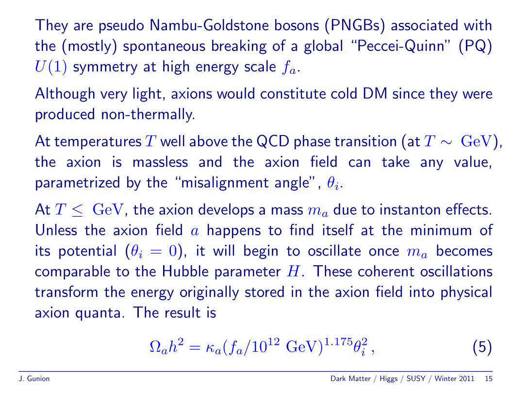
They are pseudo Nambu-Goldstone bosons (PNGBs) associated with

the (mostly) spontaneous breaking of a global “Peccei-Quinn” (PQ)

U(1) symmetry at high energy scale fa.

Although very light, axions would constitute cold DM since they were

produced non-thermally.

At temperatures T well above the QCD phase transition (at T ∼ GeV),

the axion is massless and the axion field can take any value,

parametrized by the “misalignment angle”, θi.

At T ≤ GeV, the axion develops a mass ma due to instanton effects.

Unless the axion field a happens to find itself at the minimum of

its potential (θi = 0), it will begin to oscillate once ma becomes

comparable to the Hubble parameter H. These coherent oscillations

transform the energy originally stored in the axion field into physical

axion quanta. The result is

Ωah2 = κa(fa/1012 GeV)1.175θ2i , (5)


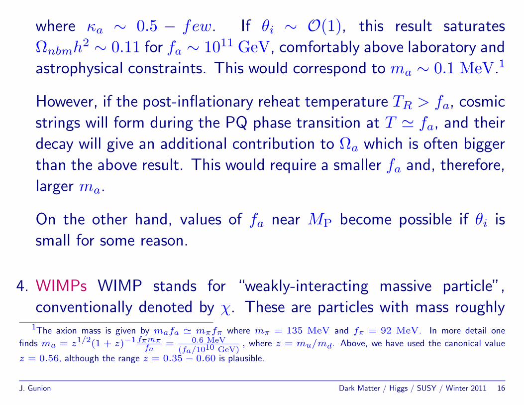
where κa ∼ 0.5 − few. If θi ∼ O(1), this result saturates

Ωnbmh2 ∼ 0.11 for fa ∼ 1011 GeV, comfortably above laboratory and

astrophysical constraints. This would correspond to ma ∼ 0.1 MeV.1

However, if the post-inflationary reheat temperature TR > fa, cosmic

strings will form during the PQ phase transition at T ' fa, and their

decay will give an additional contribution to Ωa which is often bigger

than the above result. This would require a smaller fa and, therefore,

larger ma.

On the other hand, values of fa near MP become possible if θi is

small for some reason.

4. WIMPs WIMP stands for “weakly-interacting massive particle”,

conventionally denoted by χ. These are particles with mass roughly1The axion mass is given by mafa ' mπfπ where mπ = 135 MeV and fπ = 92 MeV. In more detail one

finds ma = z1/2(1 + z)−1fπmπfa

= 0.6 MeV(fa/1010 GeV)

, where z = mu/md. Above, we have used the canonical value

z = 0.56, although the range z = 0.35− 0.60 is plausible.


between few GeV and few TeV, and with cross sections of

approximately weak strength.

Within standard cosmology, their present relic density can be calculated

reliably if the WIMPs were in thermal and chemical equilibrium with

the hot soup of Standard Model (SM) particles after inflation. In

this case, their density would become exponentially (Boltzmann)

suppressed at T < mχ.

The WIMPs therefore drop out of thermal equilibrium (freeze out)

once the rate of reactions that change SM particles into WIMPs or

vice versa,

rate ∝ nWIMP × σA × vrel (6)

becomes smaller than the Hubble expansion rate of the Universe.

Here, nWIMP is the number density of WIMPs, σA is the cross

section for WIMP-pair-annihilation to SM particles, and vrel is the

relative velocity of the annihilating WIMPs.


After freeze out, the co-moving WIMP density remains essentially

constant; if the Universe evolved adiabatically after WIMP decoupling,

this implies a constant WIMP number to entropy density ratio.

Their present relic density is then approximately given by (ignoring

logarithmic corrections)

Ωχh2 ' const.× T 30

M3P〈σAv〉

' 0.1 pb · c〈σAv〉

. (7)

Here T0 is the current CMB temperature, MP is the Planck mass, c is

the speed of light, σA is the total annihilation cross section of a pair

of WIMPs into SM particles, v is the relative velocity between the two

WIMPs in their cms system, and 〈. . .〉 denotes thermal averaging.

Freeze out happens at temperature TF ' mχ/20 almost independently

of the properties of the WIMP. This means that WIMPs are already

non-relativistic when they decouple from the thermal plasma; it also


implies that Eq. (7) is applicable if TR > TF .

Notice that the 0.1 pb in Eq. (7) contains factors of T0 and MP;

it is, therefore, quite intriguing that it happens to come out near

the typical size of weak interaction cross sections. This is called the

WIMP Miracle.

WIMP Candidates

Heavy neutrino

The seemingly most obvious WIMP candidate is a heavy neutrino.

However, an SU(2) doublet neutrino will have too large a cross

section and, therefore, too small a relic density if its mass exceeds

mZ/2, as required by LEP data.

One can suppress the annihilation cross section, and hence increase

the relic density, by postulating mixing between a heavy SU(2)


doublet and some sterile SU(2)× U(1)Y singlet neutrino. However,

one also has to require the neutrino to be stable; it is not obvious

why a massive neutrino should not be allowed to decay.

LSP

The currently best motivated WIMP candidate is, therefore, the

lightest superparticle (LSP) in supersymmetric models with exact

R-parity (which guarantees the stability of the LSP).

Searches for exotic isotopes imply that a stable LSP has to be neutral.

This leaves basically two candidates among the superpartners of

ordinary particles:

(a) a sneutrino (supersymmetric partner of a neutrino),

(b) and a neutralino (a mixture of the spin-1/2 supersymmetric partners

of the γ, Z gauge bosons and the two neutral Higgs bosons of the

minimal supersymmetric model plus, possibly, others).


Sneutrinos

Sneutrinos have quite large annihilation cross sections; their masses

would have to exceed several hundred GeV for them to make good

DM candidates.

This is uncomfortably heavy for the lightest sparticle, in view of

naturalness arguments.

Moreover, the negative outcome of various WIMP searches (see

below) rules out ordinary sneutrinos as a primary component of the

DM halo of our galaxy. (In models with gauge-mediated SUSY

breaking, the lightest messenger sneutrino could make a good WIMP.

)

Neutralinos

The most widely studied WIMP is therefore the lightest neutralino.

Detailed calculations (some of which we shall do) show that the


lightest neutralino will have the desired thermal relic density Eq. (7)

in at least four distinct regions of parameter space:

(a) χ could be (mostly) a bino or photino (the superpartner of the

U(1)Y gauge boson and photon, respectively), if both χ and some

sleptons have mass below ∼ 150 GeV;

(b) if mχ is close to the mass of some sfermion (so that its relic density

is reduced through co-annihilation with this sfermion);

(c) if 2mχ is close to the mass of the CP-odd Higgs boson present in

supersymmetric models;

(d) if χ has a large higgsino or wino component.

Other WIMP Models

(a) Many nonsupersymmetric extensions of the Standard Model also

contain viable WIMP candidates. Examples are the lightest T -

odd particle in Little Higgs models with conserved T -parity, or

technibaryons in scenarios with an additional, strongly interacting


(technicolor or similar) gauge group.

(b) Models where the DM particles, while interacting only weakly with

ordinary matter, have quite strong interactions within an extended

dark sector of the theory. These were spurred by measurements by

the PAMELA, ATIC and Fermi satellites indicating excesses in the

cosmic e+ and/or e− fluxes at high energies.

However, these excesses are relative to background estimates

that are clearly too simplistic (e.g., neglecting primary sources of

electrons and positrons, and modeling the galaxy as a homogeneous

cylinder).

Moreover, the excesses, if real, are far too large to be due to usual

WIMPs, but can be explained by astrophysical sources.

It therefore seems unlikely that they are due to Dark Matter.

(c) Although thermally produced WIMPs are attractive DM candidates

because their relic density naturally has at least the right order of

magnitude, non-thermal production mechanisms have also been


suggested, e.g., LSP production from the decay of some moduli

fields, from the decay of the inflaton, or from the decay of Q

balls (non-topological solitons) formed in the wake of Affleck-Dine

baryogenesis.

Although LSPs from these sources are typically highly relativistic

when produced, they quickly achieve kinetic (but not chemical)

equilibrium if TR exceeds a few MeV (but stays below mχ/20).

They therefore also contribute to cold DM.

DM Detection

• Primary black holes (as MACHOs), axions, and WIMPs are all (in

principle) detectable with present or near-future technology. This was

presumably what some of you learned about in the fall quarter.

• There are also particle physics DM candidates which currently seem

almost impossible to detect, unless they decay; the present lower


limit on their lifetime is of order 1025− 1026 s for 100 GeV particles.

These include:

1. the gravitino (the spin-3/2 superpartner of the graviton),

2. states from the hidden sector thought responsible for supersymmetry

breaking, and

3. the axino (the spin-1/2 superpartner of the axion).


General Relativity Basics

• The Metric:

The fundamental quantity is the metric gαβ. Consider the curves

xα(p) through a point P in Riemann space (p = curve parameter).

At any given point there will be a set of tangent vectors that indicate

how xα is changing as you move along the curve: ds = dxαeα.


The length of ds (along the curve p) is given by

ds2 = ds ·ds = (dxαeα) · (dxβeβ) = (eα ·eβ)dxαdxβ ≡ gαβdxαdxβ .

(8)

An arbitrary vector can be defined at a given location P in terms of

the tangent vectors at location P : A = Aµeµ.

• Parallel Transport:

At any given point on the curve, we can define a vector A(P) in

terms of the current tangent basis: A(P ) = Aµeµ. If we now move

to a new point Q on the curve, A(Q) will in general change, but

the question is by how much and how we should define that change.

Parallel transport of A is defined by saying that A(Q) should have

the same orientation (and length) with respect to the new tangent

basis as did A(P ) with respect to the previous tangent basis.


Figure 1: Conceptual denition of parallel displacement of a vector along a curve xσ(p) in Riemann

space. First, an ordinary parallel displacement in the flat embedding space (resulting in the dashed

arrows). Then followed by projection on the local tangent space. The process is repeated in

infinitesimal steps.

The amount of change of A not associated with maintaining same

orientation with respect to the local tangent space is defined as

dA = A(Q)−A′(Q) = d(Aµeµ) = (dAµ)eµ +Aµ(deµ) . (9)


In other words, dA may be interpreted as the intrinsic change of A,

after correction for the “irrelevant” change in the orientation of the

tangent space.

In any case, the important point is that after the move to the new

location on the curve, there will be a new set of basis vectors. The

change in the tangent vectors is defined via the Christoffel symbol:

deµ = Γαµβdxβeα . (10)

In terms of the Christoffel symbols, we have

dA = (dAµ + ΓµνσAνdxσ)eµ ≡ (DAµ)eµ . (11)

Parallel transport would correspond to maintaining DAµ/dp = 0 as

we move along the curve parametrized by p.

• Geodesics:


A geodesic is a line that is “as straight as possible” on a curved

surface. We say that a curve xµ(p) is a geodesic when the tangent

vector xµ ≡ dxµ/dp remains a tangent vector under parallel transport

along xµ(p). According to Eq. (11), this means we require

D

Dp

(dxµ

dp

)= 0, ⇒ xµ + Γµνσx

νxσ = 0 . (12)

Now, Eq. (12) can also be derived from a variational principle. The

simplest is δ∫sdp = 0 (i.e. the shortest path in terms of ds). This

is equivalent to δ∫s2dp = 0, or

δ

∫Ldp = 0, with L(xα, xβ) =

(ds

dp

)2

= gαβxαxβ . (13)


The solution is determined by the Euler-Lagrange equations

∂L

∂xλ− d

dp

(∂L

∂xλ

)= 0 . (14)

Now, ∂L/∂xλ = gαβ,λxαxβ since only gαβ depends on xµ. Then,

by using ∂xα/∂xλ = δαλ one gets ∂L/∂xλ = 2gαλxα. Substituting

these in to the Euler Lagrange equation gives:

gαβ,λxαxβ = ˙2(gαλxα) = 2(gαλ,βxβxα + gαλx

α) , (15)

or

gαλxα +

12(2gαλ,β − gαβ,λ)xαxβ = 0 . (16)

It is useful to write

2gλα,βxαxβ = gλα,βxαxβ+gλβ,αxβxα = (gλα,β+gλβ,α)xαxβ . (17)


Then, multiplying Eq. (16) by gµλ and substituting the above, we

obtain

xµ +12gµλ(gλα,β + gλβ,α − gαβ,λ)xαxβ = 0 . (18)

Comparing to Eq. (12), we conclude that the Christoffel symbols are

intimately connected to the metric tensor, the relation being

Γµαβ =12gµλ(gλα,β + gλβ,α − gαβ,λ). (19)

The Lagrangian method provides the quickest derivation of the above

relation and we have sketched it so that we can use it again when

we come to the Robertson-Walker metric appropriate to the Early

Universe.

• Riemann Tensor, Ricci Tensor, ....:

Various subsidiary quantities employed in General Relativity can be

defined in terms of the Christoffel symbol.


First, there is the Riemann Tensor:

Rαβγδ = Γαβδ,γ − Γαβγ,δ + ΓµβδΓαµγ − ΓµβγΓ

αµδ . (20)

From the Riemann Tensor one finally obtains the Ricci Tensor (or

curvature tensor) and the scalar curvature:

Rµκ = Rλµλκ , R = Rµµ . (21)

These are all related to the intrinsic curvature of space as follows.

Let us imagine parallel transport of a vector A from P to R along

two paths: 1 = (PQR) and 2 = (PSR) (see figure).


For each piece we write dAµ = −fσ(x)dxσ with fσ(x) = ΓµνσAν.

Then,

Aµ1 −Aµ2= −fσ(x)dξσ − fσ(x+ dξ)dησ + fσ(x)dησ + fσ(x+ dη)dξσ

' −fσdξσ − fσdησ − fσ,λdξ

λdησ + fσdησ + fσdξ

σ + fσ,λdηλdξσ

= (fσ,λ − fλ,σ)dξσdηλ

= RµαλσAαdξσdηλ . (22)

One easily verifies that Rαµνσ is zero in a flat space for any choice

of the co-ordinates. The above equation then implies that parallel

transport along a closed path leaves a vector unchanged. But, in

a curved space the orientation of the vector will have changed. In

4 dimensions, after using symmetries, one finds that Rανρσ has 20

independent components. Further, all contractions of Rανρσ, i.e. Rµν,are either zero or equal, apart from a sign.


• Einstein’s Equations:

Einsteins equations are stated in terms of the Einstein Tensor

Gµν ≡ Rµν −12gµνR . (23)

They are

Gµν − Λgµν = −8πGTµν (24)

where Λ is the cosmological constant.

There are a number of solutions to Einsteins equations for Tµν = 0.

• One is of course the standard Minkowski metric.

• However, we are interested in solutions that have intrinsic curvature.


The Basics of the Universe

• An important observation is that the universe is isotropic. The

distribution of matter in space is statistically the same in all

directions, and also as a function of distance, i.e. within redshift

subclasses.

• There are obvious evolution effects. The morphology of the systems

changes gradually with distance.

• Hubble, in 1929, demonstrated that the universe expands with

time. All galaxies move away from us on average with a velocity

proportional to the distance, but independent of direction. This

universal expansion is referred to as the Hubble flow:

v = H0d (25)


with H0 = 100h km s−1Mpc−1, where h = 0.71± 0.04 as measured

by WMAP. In physical units,

H0 = (2.3± 0.1)× 10−18s−1 . (26)

The peculiar velocities of the systems within the Universe, i.e. the

deviations from the Hubble flow, are generally small, <∼ 500 km s−1.

The Hubble flow is thus ’cold’ and this is because the universe cools

adiabatically.

• Coordinates:


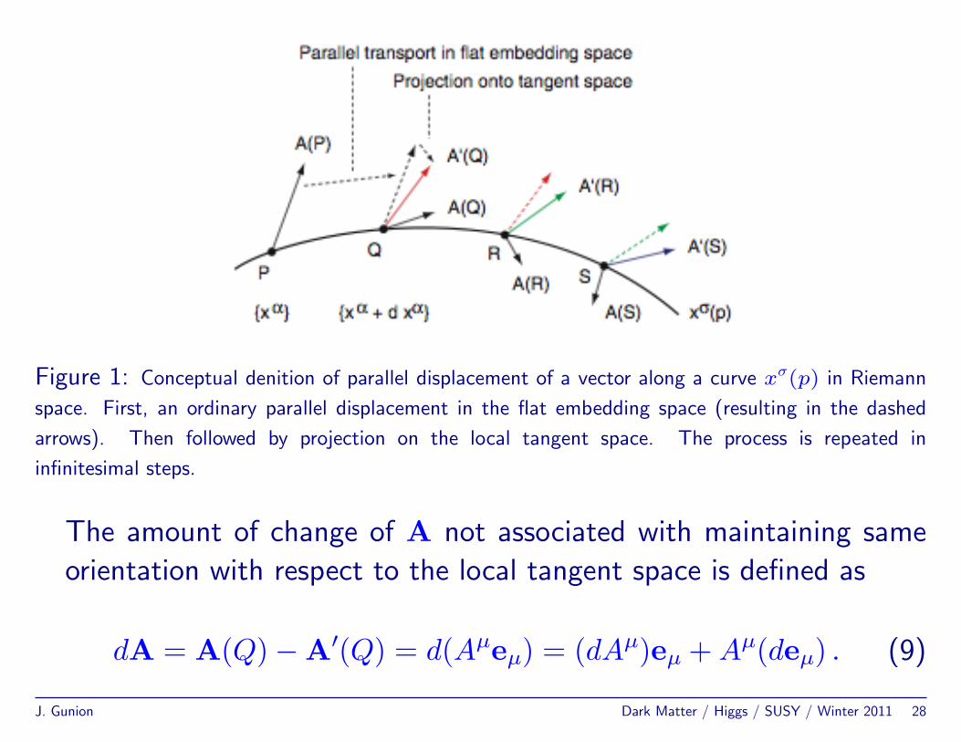
Figure 2: A picture of the spacetime of the universe. Our present position is A0. Also indicated is

our world line and our past light-cone. The wordlines of a few other galaxies (vertical lines), B and

C, are also shown. Finally, a hypothetical inhomogeneity (“giant cleft”) that we might get to see in

the future is shown.

– We are only able to see events located within or on our past light-

cone. We experience our light-cone as a series of nested, ever-

larger concentric spherical shells around us, showing an increasingly

younger section of the universe.


– Because of the observed isotropy, each shell Σ(ti) must be on

average homogenous.

– Due to our limited technological capabilities, we have not yet been

able to detect signals from the early universe, i.e. from the most

distant shells (the shaded region at the bottom of the figure).

• We now make assumptions about the part of space-time that is

outside our past light-cone and therefore unobservable.

To that end, we use the Cosmological Principle, which states that

we (A0) occupy no special position in the universe, and that other

observers B0 and C0 see on average the same universe as we do.

Hence, if we translate our light-cone sideways, the aspect of the

shells Σ(ti) would not change, apart from statistical fluctuations (the

so-called cosmic variance).

The implication is then that every subspace at t = const. is isotropic

and homogeneous on average.


Further, the Cosmological Principle and the isotropy of the universe

imply then that the universe as a whole is homogeneous.

• The definition of “rest”: We are free to adopt any definition we like,

but there is one that stands out as very natural: a test mass is at

rest if it does not move with respect to the Hubble flow.

That means the spatial co-ordinates of galaxies are constant (ignoring

their peculiar velocities).

Their wordlines are straight vertical lines in the figure, which is a

coordinate picture and contains no information about the geometry.

Due to the expansion of the universe, the geometrical distance

between B0 and C0 is larger than between B1 and C1.

It remains possible that the spacetime that we shall see in the future

contains huge inhomogeneities, and that the Cosmological Principle

will eventually prove to be incorrect, e.g. the giant cleft of the figure


could appear.

Presently, however, the assumption that every subspace t = const. is

homogeneous and isotropic is adequate.

• The first step to a definite coordinate system:

It can be shown that one can always define a time that is separate

from spatial slices in such a way that

ds2 = (dx0)2 + gikdxidxj . (27)

These are called Gaussian co-ordinates.

The essence of Gaussian co-ordinates is that the world lines of

a selected set of freely falling test masses are taken as the co-

ordinate lines of the co-ordinate system and these lines remain always

orthogonal to the sub-spaces t = const.


In cosmology, the sections t = const are snapshots of the homogeneous

and isotropic universe, and the selected test masses are the galaxies.

Because these are at rest (dxi = 0) it follows that dτ ≡ ds = dt.

This must be so because otherwise a subspace t = const would not

be homogeneous.

• Metric and spatial structure:

In order to describe an expanding universe, it is clear that the metric

must depend on x0, and that dependence must be the same for every

gik as otherwise anisotropies would develop. The implication is that

we can write

ds2 = (dx0)2 + S2(t)aikdxidxk , (28)

with aik = const in time.

We may simplify aik by noting that the space is certainly spherically

symmetric around an (arbitrarily chosen) origin. The result (after a


bit of argumentation and rescalings that I omit) is that we can write

ds2 = (dx0)2 − S2(t)(e2λ(r)dr2 + r2dΩ

), (29)

To find λ(r) we compute the total (spatial) curvature 3R = Rii of the

t = const subspace when S(t) = 1. One finds (using techniques of

geodesics, that we will come to shortly, in order to get the Christoffel

symbols)

3R = 2(

2λ′

r− 1r2

)e−2λ +

2r2

=2r2

(1− d

dr

[re−2λ

]). (30)

From this it follows that

d

dr

[re−2λ

]= 1− 1

23R r2 . (31)

Now 3R must be constant as a function of r because the space


t = const is homogeneous.

We can then integrate to obtain

e−2λ = 1− 16

3R r2 +A

r. (32)

The integration constant A should be 0; otherwise the co-ordinates

would not be locally flat at r = 0. Thus,

e2λ =1

1− kr2, (33)

where we have defined 3R ≡ 6k. In this way, we arrive at ...

• The Robertson-Walker (RW) metric: It takes the form (in terms of

the “co-moving” coordinates (r, t, θ, φ))

ds2 = dt2 − S2(t)[

dr2

1− kr2+ r2dθ2 + r2 sin2 θdφ2

](34)


This is the metric for a space with homogeneous and isotropic spatial

sections. S(t) is the “cosmic scale factor”. With an appropriate

rescaling of coordinates, we can choose k = +1, −1 or 0 for spaces

of constant positive, negative or zero curvature, respectively.

The coordinate r is dimensionless and ranges from r = 0 to r = 1if k = 1. In this case, there is a singularity at r = 1 — one cannot

consider “distances” r × S(t) larger than the cosmic scale factor,

S(t), at time t. For k = 1,

– the circumference of a one-sphere (a circle at constant φ and r) is

as expected — 2πS(t)r;– the area of a two-sphere at constant r is as expected — 4πS2(t)r2;– however, the physical radius of such one and two spheres is defined

in terms of∫ds = S(t)

∫ r0

dr′√1−kr′ 2

rather than S(t)r.

The time coordinate being employed is just the proper (or clock)

time measured by an observer at rest in the comoving frame, i.e.


(r, θ, φ) = const.. As stressed earlier, observers at rest in the

comoving frame remain at rest, i.e. (r, θ, φ) remain unchanged, and

observers initially moving with respect to this frame will eventually

come to rest in it.

Further, if one introduces a homogeneous, isotropic fluid initially

at rest in this frame, the t = const hypersurfaces will always be

orthogonal to the fluid flow, and will always coincide with the

hypersurfaces of both spatial homogeneity and constant fluid density.

The above RW form gives the metric entries:

g00 = 1, grr = − S2(t)(1− kr2)

, (35)

gθθ = −S2(t)r2, gφφ = −S2(t)r2 sin2 θ . (36)

Finally, from the RW metric form, ones finds the Ricci tensor


components and Ricci scalar that we will shortly need:

R00 = 3S

S, Rij =

[S

S+ 2

S2

S2+

2kS2

]gij, R = 6

[S

S+S2

S2+

k

S2

](37)

where a ≡ ∂a∂t . However, in the derivation below, we will need to

denote (as before) a = dadp and temporarily use a′ for ∂a∂t .

Derivation:

One can employ the brute force approach of computing the Christoffel

symbols directly from Eq. (19).

Alternatively, we can employ the definition of the Christoffel symbol in

terms of geodesics. Recall that a geodesic is defined by δ∫Ldp = 0,

where

L = gαβxαxβ = (x0)2 − S2r2

1− kr2− S2r2θ2 − S2r2 sin2 θφ2 . (38)


We emphasize again that x0 = ct, x1 = r, x2 = θ and x3 = φ are

considered to be functions of the curve parameter p. The scale factor

S depends on t, i.e. on x0. All x0 dependence of L is in S and we

will also encounter S′ = dS/dx0 and S′′ = d2S/dx0 2.

The Euler Lagrange equations resulting from the variational principle

are those given earlier:

∂L

∂xλ− d

dp

(∂L

∂xλ

)= 0 . (39)

We apply these in turn to get the Γλαβ Christoffel symbols.

1. Γ0αβ.


Applying for λ = 0, i.e. requiring ∂L/∂x0 = ddp(∂L/∂x

0) gives

− 2SS′(

r2

1− kr2+ r2θ2 + r2 sin2 θφ2

)=

d

dp(2x0) = 2x0 (40)

or

x0 + SS′(

r2

1− kr2+ r2θ2 + r2 sin2 θφ2

)= 0 . (41)

This may be compared to the definition of the Christoffel symbol

in

xµ + Γµνσxνxσ = 0 (42)

for the case of µ = 0, yielding (using the notation 1 = r, 2 = θ

and 3 = φ)

Γ011 =

SS′

1− kr2, Γ0

22 = SS′r2, Γ033 = SS′r2 sin2 θ , (43)

and all other Γ0αβ = 0. Note that Γ0

ij = −S′

S gij.


2. Γ2αβ.

For this, we employ the Euler Lagrange equation for λ = 2:

∂L/∂θ = ddp(∂L/∂θ) which gives

− 2S2r2 sin θ cos θφ2 =d

dp(−2S2r2θ)

= −4S2rrθ − 2S2r2θ − 4SS′x0r2θ .(44)

Dividing by −2S2r2 in order to have 1 × θ, the above equation

reduces to

θ +2rrθ − sin θ cos θφ2 + 2

S′

Sx0θ = 0 , (45)

from which we read

Γ212 = Γ2

21 =1r, Γ2

33 = − sin θ cos θ , Γ202 = Γ2

20 =S′

S, (46)


all other Γ2... being zero.

3. Γ3αβ.

For λ = 3, Euler-Lagrange reads ∂L/∂φ = ddp(∂L/∂φ) which gives

0 =d

dp(−2S2r2 sin2 θφ)

= −4S2rr sin2 θφ− 4S2r2 sin θ cos θθφ−2S2r2 sin2 θφ− 4SS′r2 sin2 θx0φ . (47)

Dividing by −2S2r2 sin2 θ gives

φ+2rrφ+ 2

S′

Sx0φ+ 2

cos θsin θ

θφ = 0 , (48)

from which we read

Γ313 = Γ3

31 =1r, Γ3

23 = Γ332 = cot θ , Γ3

03 = Γ330 =

S′

S, (49)


with all other Γ3... = 0.

4. Γ1αβ.

This is the messiest case. We have

∂L

∂r= −S2r2(−1)

−2kr(1− kr2)2

− S22rθ2 − S22r sin2 θφ2(50)

d

dp

(∂L

∂r

)=

d

dp

(−2S2r

(1− kr2)

)=

−2S2r

(1− kr2)− 2S2r(−1)

−2krr(1− kr2)2

− 4SS′x0r

(1− kr2).(51)

Equating and isolating r we arrive at

r+kr

(1− kr2)r2− (1− kr2)r(θ2 + sin2 θφ2) + 2

S′

Sx0r = 0 , (52)


from which we read

Γ111 =

kr

1− kr2, Γ1

22 = −(1− kr2)r ,

Γ133 = −(1− kr2)r sin2 θ , Γ1

01 = Γ110 =

S′

S, (53)

all other Γ1... = 0.

From the above results for Γi..., you will find that Γi0j = S′

S δij.

I won’t go into deriving the Riemann and Ricci tensors. Results for

the latter were already given earlier. For the Riemann tensor one

finds the following

R0101 = − SS′′

1−kr2 R0202 = −Sr2S′′

R0303 = −Sr2 sin2 θS′′ R1212 = S2r2(S′ 2+k)1−kr2

R1313 = S2r2 sin2 θ(S′ 2+k)1−kr2 R2323 = S2r4 sin2 θ(S′ 2 + k)

(54)


Finally, let me remind you again that the prime indicates derivative

with respect to time above.

If we denote the spatial part of the metric as d~l2 = gijdxidxj. We

can work out the three-dimensional Riemann tensor, Ricci tensor and

Ricci scalar, denoted by 3Rijkl,3Rij and 3R with the results

3Rijkl =k

S2(t)(gikgjl − gilgkj)

3Rij =2kS2(t)

gij

3R =6kS2(t)

. (55)

The last of these agrees with the identification of 3R = 6k for

S(t) = 1 used when we derived the RW metric. The latter two

results are also obtained by simply dropping all time derivatives in

Rµν and R.


• Kolb-Turner Notation:

Since I will be following some of their material, I note that they have

a notation in which S(t) is replaced by R(t) and they write Einstein’s

equations as Gµν = +8πGTµν, but their conventions are such that

their Gµν has a sign that is opposite that employed earlier and so the

final equations are the same. Of course, in their book and from here

on a = ∂a∂t .

At this point, we will switch to Kolb-Turner notation, i.e. S → R, but

maintain the preceding conventions for the signs of the Friedmann

Tensor, Ricci Tensor and curvature and Einstein equations.

In the next few sections, I will largely follow the relevant chapters

3 and 5 of the Kolb and Turner monograph. I have also used

some notes on this same kind of material prepared by B. Grzadkowski

(http://www.fuw.edu.pl/ bohdang/wyklady/Cosmology/cosmo 09 10.html) and by A. Lewis

(http://cosmologist.info/teaching/EU/notes EU1 thermo.pdf). The material up to this


point came from the relevant reviews in the Reviews of Particle

Properties and from a variety of standard texts. In many places I have

updated some things and added additional material/explanations.

• Time, Kinematics and Red-Shift:

A fundamental question is “for a comoving observer with coordinates

(r0, θ0, φ0), for what values of (r, θ, φ) would a light signal emitted

at t = 0 reach the the observer at, or before, time t?” The answer is

determined by the metric. The furthest distance is referred to as the

Horizon, with H as a subscript.

A light signal satisfies the geodesic equation ds2 = 0. Because of

the homogeneity of space, we may choose r0 = 0. Geodesics passing

through r0 = 0 are lines of constant θ and φ. Thus, a light signal

emitted from position (rH, θ0, φ0) at t = 0 will reach r0 = 0 in a

time t determined by setting ds2 = 0 as we move along the geodesic


which means requiring

dt =R(t)dr√1− kr2

(56)

as we move along the geodesic. Integrating, we get the following

consistency requirement for t:∫ t

0

dt′

R(t′)=∫ rH

0

dr√1− kr2

. (57)

The proper distance to the horizon measured at time t,

dH(t) =∫ rH

0

√grrdr (58)

is related to the above by

dH(t) = R(t)∫ t

0

dt′

R(t′). (59)


For standard cosmology, dH(t) ∼ t is finite.

So, now let us look at a photon travelling along a geodesic. We

describe its 4-momentum as usual as pµ = (E, ~p), where we can

assume that ~p is entirely in the radial direction. The evolution of pµ

is then given by the geodesic equation

dpµ = −Γµναpνdxα . (60)

For µ = 0 and ~p = rpr, this reduces to

dE = −Γ0rrp

rdr = − RR

(1− kr2)prdr . (61)

Now, we must be careful to relate pr to E correctly by using

gµνpµpν = E2 − grrp

rpr = E2 − R2

(1− kr2)prpr = 0 ., (62)


which yields pr = E√

1− kr2/R. Substituting this and the geodesic

constant θ, φ relation of (see Eq. (56)) dr = dt√

1− kr2/R into the

dE equation, we obtain

dE = − RR

1− kr2

(E√

1− kr2

R

)(dt√

1− kr2

R

)⇒ E

E= −R

R.

(63)

The solution is obviously that E ∝ 1R. Since for a photon λ ∝ 1/E,

we find λ ∝ R.

The standard “red-shift”, z, is defined in terms of the ratio of the

detected wavelength (at t0) to the emitted wavelength at the earlier

time t1:

1 + z ≡ λ0

λ1=R(t0)R(t1)

. (64)

Any increase in R(t) with t for t0 > t1 leads to a red-shift of the light

from sources that are distant from the observer, since such sources


emitted light at earlier times when R(t) was smaller..

For a particle with mass, for uµ ≡ dxµ/ds = (γ, γ~v) (~v being the

usual velocity) a similar procedure gives

˙|~u||~u|

= −RR, ⇒ |~u| ∝ R−1 . (65)

implying that a particle with mass will eventually come to rest in the

comoving frame.

• The stress energy tensor: To be consistent with the symmetries of the

metric, Tµν must be diagonal. By isotropy the spatial components

must be equal. The simplest realization is

Tµν = diag(ρ,−p,−p,−p) (66)

i.e. as for a perfect fluid characterized by a time-dependent energy

density ρ(t) and pressure p(t).


• The 1st law of thermodynamics: Given the above form, the first law

follows from Tµν;ν = 0 and takes the physically expected form

d(ρR3) = −pd(R3) , or equivalently dρR3 = −(p+ ρ)d(R3) .(67)

The first form simply says that the change in energy in a co-moving

volume element, d(ρR3), is equal to minus the pressure times the

change in volume, −pd(R3).

• Equation of state implications:

One writes p = wρ. In simple cases, w is independent of time. If so,

then Eq. (67) reduces to dρρ = −(1 +w)d(R

3)R3 , for which the solution

is

ρ ∝ R−3(1+w) . (68)

Important cases are:

1. Radiation Dominance (RD): (p = 13ρ) i.e. w = 1/3 ⇒ ρ ∝ R−4


2. Matter Dominance (MD): (p = 0) i.e. w = 0 ⇒ ρ ∝ R−3

3. Vacuum Energy Dominance (VD): (Tµν ∝ gµν = diag(1, 1, 1, 1)) for

which p = −ρ, i.e. w = −1 ⇒ ρ ∝ constant

At the earliest times after inflation the universe was radiation

dominated. By radiation here, we mean any relativistic object,

including relativistic matter as well as photons.

At intermediate times, earlier than the present epoch, the universe

was matter dominated.

The final situation depends upon whether there is a cosmological

constant or equivalent. If not, then the universe would remain

matter dominated (or curvature dominated if k 6= 1). However,

measurements suggest that something like a small cosmological

constant is taking over slowly.

During inflation, the universe was dominated by vacuum energy (not

the current vacuum energy, but something much larger).


• The Einstein equation:

The 0− 0 and i− i components of

Rµν −12gµνR = −8πGTµν (69)

read:

R2

R2+

k

R2=

8πG3ρ , (70)

2R

R+R2

R2+

k

R2= −8πGρ . (71)

The first equation above is the “Friedmann Equation”. The difference

between the above two equations yields:

R

R= −4πG

3(ρ+ 3p) . (72)


Today, R ≥ 0. If in the past ρ + 3p was always > 0 (radiation or

matter) then R was always < 0, and thus at some finite time in the

past R must have been equal to 0. This time corresponds to the

“big-bang”and is usually identified with t = 0.

Eqs. (67), (70) and (71) are not independent (being related by

Bianchi identities). Usually, it is most convenient to take Eqs. (67)

and (70) as the independent equations.

• Hubble parameter and related:

The Hubble parameter is H ≡ RR in terms of which the Friedmann

equation,R2

R2+

k

R2=

8πG3ρ , (73)

can be rewritten in the form

k

H2R2=

ρ

3H2/8πG− 1 ≡ Ω− 1, (74)


where

Ω ≡ ρ

ρcwith ρc =

3H2

8πG. (75)

Since H2R2 ≥ 0, we have the correspondence

k = +1 ⇒ Ω > 1 closed

k = 0 ⇒ Ω = 1 flat

k = −1 ⇒ Ω < 1 open . (76)

Now, it is important to note that H is not independent of time. We

will denote the current value by H0. We will also use R0 for the

current scale factor R(t0) at current time t = t0. As we saw earlier,R0R ≡ 1 + z, R = R(t) being the scale factor at some earlier time, t.

Of course, 1 + z is then the red-shift we see for light coming from

some earlier time t from a distant galaxy. In the Ω ≥ 1 cases, it is

conventional to define the zero of time to be that time when R→ 0(and z → ∞). Of course, technology and physics prevent us from


seeing all the way back to t = 0.

Now, kH2R2 = Ω − 1 is valid for all times. However, Ω − 1 and

ρc = 3H2

8πG are not constant. They change as the Universe expands.

At early times, we will see that a self-consistent solution to the

Friedmann equation will imply that the curvature term k/R2 is

negligible compared to (R/R)2 = H2.

Assuming this for the moment, the Friedmann equation written as

in Eq. (70) gives R2

R2 ∼ 8πG3 ρ which gives H2 ∝ R−3 in the (MD)

case or H2 ∝ R−4 in the (RD) case (see earlier summary), giving

k/(H2R2) ∝ R (MD) , R2 (RD).

Using the above scalings, at early times kH2R2 = Ω− 1 with k = +1

gives

|Ω− 1| ∼R/R0 = (1 + z)−1 (MD)(REQ/R0)(R/REQ)2 ' 104(1 + z)−2 (RD)

(77)


where REQ ' 10−4R0 is the value of R at the transition between

matter domination and radiation domination. At early times, 1+z 1, Ω ∼ 1 and the Universe was very nearly critical. Of course, the

above equation can’t be used for small z.

Note that since the above gives kH2R2 1 at early times, this implies

that kR2 H2 at early times so that our original assumption of

neglecting the kR2 curvature term compared to H2 in the Friedmann

equation at early times is self-consistent.

Another little detail we need to get straight is the relationship of k

to actual spatial curvature.

You need to recall that we defined 3R = 6kR2(t)

earlier below Eq. (33).

(There we did the calculation for S(t), now called R(t), = 1 and

got 3R = 6k — clearly 3R scales as 1/R2(t), see Eq. (55).) Usingk

H2R2 = Ω− 1 this can be re-expressed as 3R = 6H2(Ω− 1).

From the form of the RW metric, it is clear that the effects of


spatial curvature become very significant for r ∼ |k|−1/2, so we

define a physical “radius of curvature” of the Universe, Rcurv ≡R(t)|k|−1/2 =

(6|3R|

)1/2

that is related to the Hubble radius, H−1,

by

Rcurv =H−1

|Ω− 1|1/2. (78)

When |Ω−1| is of order unity, Rcurv and H−1 are comparable; when

|Ω− 1| is very small, Rcurv H−1. What this means is that if the

Universe is close to critical density, then it has very large curvature,

i.e. is very flat.

In particular, since |Ω− 1| must have been very small at early epochs

(see above), it is safe to ignore spatial curvature in the early Universe.

Note that for the closed models, k > 0, Rcurv is just the physical

radius of the 3-sphere defined by kr2 = 1 with actual radius rR(t) =k−1/2R(t).


Finally, we note while we have scaled r such that k = +1, 0 or −1,

there are an infinity of RW models, characterized by different k but

the same physical curvature radius, Rcurv = R(t)|k|−1/2, at some

specified epoch.

That is to say, all physics is contained in the ratio k/R2 and not

separately in k.

• The Age of the Universe:

We will now show how the Friedmann equation can be integrated

to give the age of the Universe in terms of present cosmological

parameters.

Given that

ρ/ρ0 = (R/R0)−3(1+w) ∼ R−3 (MD), R−4 (RD) , (79)

the Friedmann equation, after multiplying by R2/R20, can be rewritten


in the form(R

R0

)2

+k

R20

=8πG

3ρ0R0

R= H2

0Ω0R0

R(MD) (80)

(R

R0

)2

+k

R20

=8πG

3ρ0

(R0

R

)2

= H20Ω0

(R0

R

)2

(RD) ,(81)

where the last forms used the fact that (8πG/3)ρc = H2 (see

Eq. (75)) applies at any time and in particular today so that

(8πG/3)ρ0 = (H20/ρ0 c)ρ0 = H2

0ρ0ρ0 c

= H20Ω0. Defining x = R/R0

and recalling that R0/R = 1 + z we then obtain (assuming the

Universe started with a big-bang at R = 0, or at least some very

small value, in order to set the lower limit in the following)


t ≡∫ R(t)

0

dR′

R′

= H−10

∫ (1+z)−1

0

dx

[1− Ω0 + Ω0x−1]1/2(MD)

= H−10

∫ (1+z)−1

0

dx

[1− Ω0 + Ω0x−2]1/2(RD) . (82)

If we now input the fact that currently Ω0 ∼ 1 and use the (present)

measured value of H0 ∼ h0 × (9.77 Gyr)−1 with h0 ∼ 0.7, then for

a matter dominated universe we would have

t ∼ 9.77 Gyr × h−10

23(1 + z)−3/2 ∼ 9(1 + z)−3/2 Gyr . (83)

Setting z = 0 to obtain the current age of the universe gives

t0 ∼ 9 Gyr which is too small. The reason is that we need to include


the vacuum energy or cosmological constant. The result is that the

present age is

t0 ∼23H−1

0 Ω−1/2vac ln

[1 + Ω1/2

vac

(1− Ωvac)1/2l

], (84)

where Ωvac + Ωmatter = 1 was assumed. Plugging in Ωvac = 0.75gives t0 = 14.1 Gyr, nicely consistent with what we think we know.

• The deceleration parameter:

As an aside, we now know that the deceleration parameter, called q0,

defined by

q0 ≡ −

(R(t0)R(t0)

)1H2

0

, (85)

is quite interesting. By taking the ratio of RR = −4πG

3 (ρ + 3p) to

the Friedmann equation R2

R2 + kR2 = 8πG

3 ρ and using the definition of


Ω0, we find (neglecting k/R20, a good approximation at the current

epoch)

q0 =12Ω0

[1 + 3

p

ρ

]=

12Ω0(1 + 3w) . (86)

This gives:q0 = 1

2Ω0 (MD,w = 0)q0 = Ω0 (RD,w = 1/3)q0 = −Ω0 (V D,w = −1) .

(87)

In particular, we see the standard result that in a vacuum-dominated

model the expansion is accelerating, R0 > 0, since Ω0 ∼ 1 > 0.

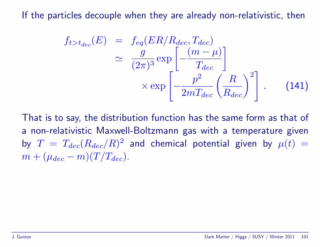
• Equilibrium Thermodynamics:

In terms of the phase space distribution function f(~p) we have:

n =g

(2π)3

∫f(~p)d3p (88)


ρ =g

(2π)3

∫E(~p)f(~p)d3p (89)

p =g

(2π)3

∫|~p|2

3E(~p)f(~p)d3p , (90)

where g is the number of internal degrees of freedom and E2(~p) =|~p|2 +m2.

For a species in kinetic equilibrium the phase space occupancy is

given by

f(~p) =1

e(E−µ)/T ± 1(91)

where µ is the chemical potential and +1 is for fermions and −1 is

for bosons. If the species is also in chemical equilibrium then its µ

is related to the chemical potentials of other species with which it

interacts. For example, if chemical equilibrium holds for i+j ↔ k+ l,we have

µi + µj = µk + µl (92)


In the relativistic limit T m and for T µ the integrals are simple

and we find

n =

(ζ(3)π2

)gT 3 (bosons)

34

(ζ(3)π2

)gT 3 (fermions)

(93)

ρ =

(π2

30

)gT 4 (bosons)

78

(π2

30

)gT 4 (fermions)

(94)

p =ρ

3. (95)

If there are any relativistic species then it is a good approximation

to use only them since the contributions from non-relativistic species

are very small (exponentially suppressed) in comparison. Thus, we


typically employ to good approximation

ρR =π2

30g∗T

4 , pR =ρR3, (96)

with

g∗ =∑

i=bosons

gi

(TiT

)4

+78

∑i=fermions

gi

(TiT

)4

. (97)

Of course, once T falls below mi we stop including particle i in the

sum. We will find that Ti = T for all particles except neutrinos.

During the radiation dominated epoch (roughly t <∼ 4 × 1010 sec)

we have ρ = π2

30g∗T4. Also recall that ρ

(3H2/8πG)= Ω, so that for

Ω ' 1 (k ' 0) we obtain

H =[8πG

3ρ

]1/2=[8πG

3π2

30g∗T

4

]1/2= 1.66

g1/2∗

MPT 2 , (98)


where MP is the Planck mass defined as MP =√

~cG = 1.22 ×

1019 GeVc = 1.22× 1022 MeV

c .

For the radiation dominated Universe we found earlier that R(t) ∝t1/2 with the consequence that H ≡ R

R = 12t. Plugging this in above

and solving for t gives

t = 0.30MP

g1/2∗ T 2

∼ 2.4

g1/2∗

(1 MeV

T (in MeV)

)2

sec , (99)

where 1 MeV is a temperature that will frequently appear in our

discussion.

Note: The above formula can’t be used to compute the age of the

universe since it is only valid for smallish times.

Units

Perhaps this is as good a time as any to make sure everyone has


the system of units under control. Everything we have written has

assumed ~ = c = 1.

Now ~c = 197.3 MeV fm where 1 fm = 10−13 cm. Then, ~c = 1implies 1 cm = 1013

197.3 MeV−1.

Further c = 1 is equivalent to 3× 1010 cm = 1 sec.

Combining, we get 1 sec = 3×1023

197.3 MeV−1.

Thus,

0.3MP

MeV2 = 0.3× 1.22× 1022 MeV−1

=0.3× 1.22× 1022(

3×1023

197.3

) sec

= 2.4 sec (100)

If you are unfamiliar with the ~c = 197.3 MeV fm equivalence,

please look work it out for yourself. It is roughly saying that 0.2 GeV


(the typical energy scale associated with the proton bound state) is

equivalent to 1/fm where the typical size of a proton is of order a

fermi.

Some other useful conversion factors are the following: 1 K =4.3668 cm−1 = 8.6170 ·10−14 GeV = 1.5361 ·10−37 g (coming from

the kB = 1 convention implicit in our f(~p) formulae); 1 Mpc =1.5637 · 1038 GeV−1; G = 6.7065 · 10−39 GeV−2; and H0 = h ×2.1317 · 10−42 GeV.

In particular, it is worth noting that the CMB temperature of 2.73 Kis equivalent to 2.73× 8.6170 · 10−14 GeV ∼ 2.35 · 10−10 MeV.

Particle Counting

1. For T MeV, only the 3 neutrino species (that we now know

are very light) and the photon are relativistic.


Since Tν = (4/11)1/3Tγ (will discuss later),

g∗( MeV) =78(3× 2)

(411

)4/3

+ 2 ' 3.36 , (101)

where we have taken account of the facts that the photon has 2

spin directions and that each neutrino has an anti-neutrino partner,

but that each neutrino has only a left-handed spin direction in the

SM (and each anti-neutrino a right-handed spin direction).

2. For 1 MeV <∼ T <∼ 100 MeV, the electron and positron are

relativistic, each having two spin directions, and Tν = Tγ = Te,

implyingg∗ =

78(3× 2) + 2 +

78(2× 2) = 10.75 . (102)

3. For T > 300 GeV, all the species in the standard model —neutrinos, photon, 8 gluons, W±, Z, 3 generations of quarks(each with 3 colors and each having an anti-quark partner) andleptons (plus anti-leptons), and 1 spin-0 Higgs boson — should be


relativistic yielding

g∗ = neutrinos+photon+charged−leptons+gluons+(W±, Z)+quarks+Higgs

(103)

as given below:

g∗ =78(3×2)+2+

78(3×2×2)+8×2+3×3+

78(3×3×2×2×2)+1 = 106.75 .

(104)

For example, for the quarks there are 3 families, 3 colors, 2 for

up+down, 2 for quark+antiquark and 2 for two spin directions.

You might ask why the gluons are not treated as massless. This is

because they are confined and have an effective mass for counting

purposes of order a GeV.

When we come to supersymmetry, there will be additional particles

to account for, especially in the very early universe when T was very

large.


Without supersymmetry the plot is

Figure 3: The evolution of g∗ with T is shown below. We will discuss g∗S shortly.

• Entropy

For most of the history of the Universe (in particular at very early

times) the reaction rates of particles in the thermal bath, Γint,


were much greater than the expansion rate, H, and local thermal

equilibrium should have applied.

In this case, the entropy per comoving volume element remains

constant, and provides a very useful “fiducial” quantity during the

expansion of the Universe.

For unit coordinate volume (r = 1) the physical volume is V = R3.

The 2nd law of thermodynamics states that (U is internal energy and

W is work)

TdS = dU − dW = d(ρV ) + pdV = d[(ρ+ p)V ]− V dρ , (105)

where ρ and p are the equilibrium energy density and pressure and

are only function of T (see explicit forms given earlier).


Now, in general,

dS(V, T ) =∂S(V, T )∂V

∣∣∣∣T

dV +∂S(V, T )∂T

∣∣∣∣V

dT . (106)

Since ρ and T depend only on T , matching this to the TdS =d(ρV ) + pdV form of the 2nd law given in Eq. (105) leads to

∂S

∂V

∣∣∣∣T

=1T

(ρ+ p) ,∂S

∂T

∣∣∣∣V

=V

T

dρ

dT. (107)

The integrability condition

∂2S

∂T∂V=

∂2S

∂V ∂T(108)

then takes the form

∂

∂T

∣∣∣∣V

[1T

(ρ+ p)]

=∂

∂V

∣∣∣∣T

[V

T

dρ

dT

](109)


which implies

− 1T 2

(ρ+ p) +1T

d

dT(ρ+ p) =

1T

dρ

dT⇒ dp

dT=

1T

(ρ+ p) . (110)

This can also be obtained by direct computation using the forms of

p(T ) and ρ(T ) given earlier. Inserting dp = dTT (ρ + p) into the 2nd

law form dS = 1Td [(ρ+ p)V ]− V dp gives

dS =1Td [(ρ+ p)V ]− V (ρ+ p)

dT

T 2= d

V

T(ρ+ p) + const.

,

(111)

so that up to a constant

S(V, T ) =V

T(ρ+ p) . (112)

Returning to the 1st law d[(ρ + p)V ] − V dp = 0 and inserting

dp = dTT (ρ + p) as obtained above, gives, after removing an overall


factor of T ,

d

[(ρ+ p)V

T

]= 0 , ⇒ dS = 0 , (113)

which is to say that (in thermal equilibrium) the entropy per comoving

volume, which is what S is, is conserved.

Note: above we implicitly assumed |µk| T for all particle species

— a very good approximation.

We can also define the entropy density

s ≡ S

V=ρ+ p

T. (114)

Using the earlier derived results

ρR =π2

30g∗T

4 , pR =ρR3, (115)


we find

s =2π2

45g∗ST

3 (116)

where

g∗S =∑

i=bosons

gi

(TiT

)3

+78

∑i=fermions

gi

(TiT

)3

. (117)

For most of the history of the Universe all particle species had a

common T and g∗S = g∗.

A useful normalization is the number of photons,

nγ =ζ(3)π2

2T 3 . (118)

Inserting this into the expression for s we find

s =π4

45ζ(3)g∗Snγ ' 1.8g∗Snγ. (119)


Today, g∗S ' 78(3× 2) 4

11 + 2 = 4311 leading to s ' 7.04nγ.

Now, conservation of S implies sR3 ∼ const. Combining with

s ∝ g∗ST3 we obtain

g∗ST3R3 = const (120)

as the Universe expands. Note that this implies that

T ∝ g−1/3∗S R−1 , (121)

yielding the familiar result that T ∝ R−1 whenever g∗S is constant.

Of course, whenever a particle species becomes non-relativistic and

“disappears” (from chemical equilibrium), its entropy is transferred

to the other relativistic particles still present in the thermal plasma,

causing T to decrease slightly less slowly.

It is useful to note that s ∝ R−3 ⇒ R3 ∝ s−1. Thus, the number of


some species in a comoving volume, N = R3n, is ∝ ns . In fact, it is

conventional to define

N ≡ n

s. (122)

For example, for a boson with n =(ζ(3)π2

)gT 3 (see earlier), using

Eq. (116) one finds

N =45ζ(3)g2π4g∗S

, T m,µ . (123)

• Decoupling of massless particles

The above does not apply to massless particles (massless with respect

to the decoupling temperature). Massless particles, that are already

decoupled from the heat bath (because they interact too weakly

— defined in a moment — with other particles) will not share in

the entropy transfer as T drops below the mass threshold for some

process.


Instead, the T for the massless species scales as T ∝ R−1.

To see this, consider a massless particle species initially in LTE which

decouples at time tdec, temperature Tdec and scale factor Rdec. The

phase space distribution at decoupling is

f(~p, tdec) =1

e(E/Tdec) ± 1. (124)

After decoupling, the energy of each massless particle is red shifted

(just like a photon) by the expansion of the Universe: E(t) =E(tdec)[R(tdec)/R(t)].

But, since the particle species has decoupled there is no longer any

“temperature” defined by thermal equilibrium and so Tdec remains as

shown in the above formula.

In addition, the number density of particles decreases due to the

expansion as n ∝ R−3.


These facts imply that in the the phase space distribution function,

f(~p) = d3n/d3p, the factors of R−3 cancel out between numerator

and denominator and f(~p, t) at time t will be precisely that of a

species in LTE with temperature T (t) = TdecRdec/R(t):

f(~p, t) = f(~pdec, tdec) = f(~pR

Rdec, tdec) (125)

=1

e( ERRdec

)/Tdec ± 1=

1e(E/T ) ± 1|

. (126)

Thus, the f for a massless particle species remains self-similar as the

universe expands, with the temperature red-shifting as R−1:

T = TdecRdecR

∝ R−1 , (127)

and not as g−1/3∗S R−1.


• Neutrinos — an example of decoupling:

Let’s now discuss the decoupling of neutrinos at about T ∼ 1 MeVand how this leads to neutrinos currently having a lower temperature

than the CMB photons.

First, the equilibrium reaction just before neutrino decoupling was

e+ + e− ↔ νi + νi. The cross section for neutrino production (via

W exchange) is roughly (for s m2W )

σweak(e+ + e−→ νi + νi) ∼(g2weak

4π

)2s

m4W

. (128)

Now s ∼ (〈E〉)2 and 〈E〉 ∼ 3T , so that for T mW

σweak(e+ + e−→ νi + νi) ∼(g2weak

4π

)2T 2

m4W

. (129)

The interaction rate Γint ≡ t−1collision = nσv, so with n ∼ T 3 and


v ∼ 1, we find

Γint ∼α2weakT

5

m4W

T 5 ∼ G2FT

5 , (130)

where GF = 1.1664× 10−5 GeV−2 is the Fermi constant.

This interaction rate should be compared to the expansion rate

H ∼ g1/2∗ T 2/MP [see Eq. (98)]:

ΓintH

∼ G2FT

5

g1/2∗ T 2/MP

∼(

T

0.7 MeV

)3

. (131)

Thus, at T <∼ 1 MeV the interactions are too slow to provide an

equilibrium between leptons and neutrinos. Neutrinos decouple from

the other SM particles and evolve separately. As we have seen above,

the neutrinos will then have a different temperature as compared to


other particles, in particular the photons. For the neutrinos we have:

Tν = TdecRdecR

∼ 1R. (132)

Now, for those species still in equilibrium,

g∗S(RT )3 = const.⇒ T ∼ (g∗S)−1/3 1R

(133)

The implication of the above is that the neutrino distribution will be

the same as if the neutrinos were still in thermal equilibrium with the

photons as long as g∗S does not change.

However, slightly below the ∼ MeV temperature at which the

neutrinos decouple, the electrons become non-relativistic, i.e. at

T ∼ me ' 0.5 MeV, and they annihilate via e+e− → γγ (the

inverse process being suppressed as the average energy decreases


below roughly 2me). As a result, the number of relativistic degrees

of freedom drops:

– for T >∼ 2me, the number of particle species in equilibrium with

photons include the photon (g = 2) and e± pairs (g = 4) for a

value of

g∗ =∑bosons

gi +78

∑fermions

gi = 2 +78× 4 =

112

; (134)

– for T 2me, the electrons and positrons have annihilated and

only the photons are in equilibrium with themselves, yielding

g∗ = 2 . (135)

For the particles in equilibrium with the photons, g∗(RT )3 (where

T = Tγ) remains constant during expansion. This implies that the

entropy that resided in the e± for T >∼ 2me must be transferred to


the photons when T falls below 2me and g∗ decreases.

We have (below “before” refers to before e± annihilation and “after”refers to after e± annihilation)

[g∗(RT )3

]before

=[g∗(RT )3

]after

⇒ 112

(RT )3before = 2(RT )3after . (136)

Thus, the e± entropy transfer increases (RTγ) by a factor of

(11/4)1/3, while RTν remains constant since the neutrinos had

already decoupled.

⇒ T

Tν=(

114

)1/3

= 1.40 (137)

just after annihilation and this ratio continues until today. Using

the currently observed CMB temperature T = Tγ = 2.73 K, we get

Tν = 1.95 K. This will create a difference between g∗ and the g∗Sthat includes the entropy contribution of the neutrinos — g∗S must


increase relative to g∗ since the entropy should not change as T is

decreased. Of course, in actuality, there is no sudden jump. The

decrease in g∗ occurs in a continuous fashion and does not lead to

an actual increase in T , but rather causes T to decrease less slowly

than R−1 . A plot is below (the g∗S indicated there includes entropy

in the neutrinos)


Using the above temperatures, we find (assuming 3 neutrino species)

g∗(today) = 2 +78× 2× 3×

(411

)4/3

= 3.36 ,

g∗S(today) = 2 +78× 2× 3×

(411

)= 3.91 . (138)

We emphasize that since the photon and neutrinos species are

decoupled, their entropies are separately conserved (which fact we

used implicitly above).

Using the above results, we can compute the present energy density

and entropy density of the photons and neutrinos:


γ ν

ρ = π2

30g∗T4 4.67 · 10−34 g cm−3 3.18 · 10−34 g cm−3

s = 2π2

45 g∗ST3 1486 cm−3 1419 cm−3

n = ζ(3)π2 gnT

3 413 cm−3 338 cm−3

Ωh2 = ρ 8πG3(H0/h)2

2.49 · 10−5 1.70 · 10−5

(139)

where I have defined

gn =∑bosons

(TiT

)3

+∑

fermions

34

(TiT

)3

= 2 photons

=34× 2× 3×

(411

)neutrinos . (140)


Additional remarks

Notice that the above situation applies whenever a massive particle

decouples when it is still relativistic, Tdec m. That is the

distribution function is “frozen” in the form of the equilibrium

distribution function feq of massless particles.

These decoupled massive particles will eventually become non-

relativistic when the temperature of the thermal bath drops below

their mass, T < m, and their energy will then be E ' m.

The distribution function and number density of the particles will

still be given by the frozen-in form corresponding to relativistic

particles, but the energy density will be that of non-relativistic

particles, ρ = nm.

This is exactly what happens for massive neutrinos.


If the particles decouple when they are already non-relativistic, then

ft>tdec(E) = feq(ER/Rdec, Tdec)

' g

(2π)3exp

[−(m− µ)

Tdec

]× exp

[− p2

2mTdec

(R

Rdec

)2]. (141)

That is to say, the distribution function has the same form as that of

a non-relativistic Maxwell-Boltzmann gas with a temperature given

by T = Tdec(Rdec/R)2 and chemical potential given by µ(t) =m+ (µdec −m)(T/Tdec).


The Expanding Universe, Non-Equilibrium processes andthe Boltzmann Equation

• Thermal equilibrium applied for much of the early history of the

Universe.

• But, there have been crucial and very interesting departures

1. neutrino decoupling

2. decoupling of the background radiation

3. primordial nucleosynthesis

4. inflation?

5. baryogenesis?

6. relic WIMPs?

7. axions?

If it were not for such departures from LTE, the present state of the


Universe would be completely specified by the present T .

The decouplings are interesting because they leave behind relics.

Our focus = relic WIMPS and related

• Once decoupled n ∝ R−3 and E, p ∝ R−1.

It is the evolution of particle distributions around the epoch of

decoupling that is particularly challenging but also particularly interesting.

Recall again the relations:

Γint >∼ H = coupled , Γint <∼ H = decoupled . (142)

But to properly predict relic abundances as a function of the

interactions and properties of the relevant particles requires a microscopic

treatment using


• the Boltzmann Equation:

L[f ] = C[f ] , (143)

where C is the collision operator and L is the Liouville operator. The

covariant, relativistic version of the Liouville operator is

L = pα∂

∂xα− Γαβγp

βpγ∂

∂pα. (144)

Specializing to the RW metric and using the fact that f is spatially

homogeneous and isotropic, f = f(|~p|, t), the α = 0 component (the

only non-trivial component) becomes

L[f ] = E∂f

∂t− R

R|~p|2 ∂f

∂E. (145)

We can now write the Boltzmann equation in terms of the number


density

n = 4π∫dpp2 g

(2π)3f(E, t) (146)

by integrating the preceding equation over the momentum. Defining

gπ = g(2π)3

, we find

gπ4π∫dpp2L[f ]

E=

dn

dt− gπH4π

∫dpp4

E

∂f

∂E(147)

=dn

dt− gπH4π

∫dEE

p3

E

∂f

∂E(148)

=dn

dt+ gπH4π

∫dE

∂(p3)∂E

f (149)

=dn

dt+ gπH4π

∫dE3p2 ∂p

∂Ef (150)

= n+Hgπ4π∫dE3p2E

pf (151)


= n+ gπH4π∫

3dpp2f (152)

= n+ 3Hn , (153)

where we identified H = RR and used m2 = E2 − p2 so that pdp =

EdE (used in several places) and integrated by parts.

Notice that in the absence of interactions, the Boltzmann equation

would reduce to:

n+ 3Hn = 0 , (154)

which is just the conservation of particles per comoving volume,

d(R3n)/dt = 0, which would apply when there are no interactions or

decays. The 3H term takes care of the dilution that comes from the

Hubble expansion.

For very massive particles (so ρ = mn, p = 0), the equation is just

the energy conservation equation.


In summary, the lhs of the integrated Boltzmann’s equation is simply

g

(2π)34π∫dpp2L[f ]

E=

1R3

d

dt(nR3) , (155)

which is the rate of change of the number of particles per comoving

volume divided by volume.

• Inputting Collisions:

On the rhs of the equation, we have

g

(2π)3

∫d3p

EC[f ] . (156)

For a general collision operator C[f ] we get a very complicated set of

coupled equations: n above would refer to that for any given particle

and∫d3pE C[f ] would involve it and all other particles.


In practice, we will be interested in focusing on a given particle, let

us say a WIMP, denoted χ, and the collision operator will be well

approximated by keeping only the χ and a limited set of particles

that remain in equilibrium with one another (only the χ is going out

of equilibrium).

It is also particularly relevant to consider two particle into two particle

processes, say χ+A→ B + C. The general case gets rather messy.

Focusing on the χ, we want the rhs of our Boltzmann equation to

correspond to minus the rate of loss of χ’s plus the rate of production

of χ’s, where the rate corresponds to the number of interactions per

unit volume per unit time.

Now, simplifying our notation to 12 → 34, reaction rates for 1+2 →3 + 4 are related to the corresponding cross section by (see p. 100,

Peskin and Schroeder)

rate(12 → 34) = n1n2|v1 − v2|σ12→34 (157)


where n1 and n2 are the number densities of particles 1 and 2; in our

case 1 = χ, 2 = A, 3 = B and 4 = C.

Meanwhile (see Eq. (4.79) of PS),

σ12→34 =1

2E12E2|v1 − v2|

∫dΠ3dΠ4|M|212→34(2π)4δ4(p1 +p2−p3−p4) (158)

with dΠ = g(2π)3

d3p2E , where g counts the degrees of freedom of the

particle and |M|2 is defined in the convention that it is averaged

over the degrees of freedom of all particles involved.

In our case, the number densities will be differentially defined as for

example n1 =∫dn1 =

∫g1

(2π)3d3p1f1. Putting the above together

gives

rate(12 → 34) =∫dΠ1dΠ2dΠ3dΠ4(2π)4δ4(. . .)|M|212→34f1f2 .

(159)


Note how the 2E1 and 2E2 factors in the denominator of the cross

section form neatly combined with the d3p1 and d3p2 to give the d3p12E1

and d3p22E2

factors that are part of dΠ1 and dΠ2. And, of course, theg1,2

(2π)3that were part of dn1,2 also work nicely to give the rest of the

dΠ1,2.

The net result is that the rhs of the Boltzmann equation for n1 is

−rate(12 → 34) + rate(34 → 12)

= −∫dΠ1dΠ2dΠ3dΠ4(2π)4δ4(p1 + p2 − p3 − p4)

×[|M|212→34f1f2 − |M|234→12f3f4

]. (160)

Now, T invariance (equivalently CP invariance) implies

|M|212→34 = |M|234→12 (161)


so that we can rewrite Eq. (160) in the form

−rate(12 → 34) + rate(34 → 12)

= −∫dΠ1dΠ2dΠ3dΠ4(2π)4δ4(p1 + p2 − p3 − p4)

×|M|212→34 [f1f2 − f3f4] . (162)

In the above derivations, we have neglected any Fermi blocking or

similar effects. The invariant matrix elements squared are averaged

over initial and final spins, and include the appropriate symmetry

factors for identical particles in the initial or final states.

There is an additional subtlety. The expressions for the cross sections

given above only apply in a collinear frame where ~v1 and ~v2 are

parallel. In thermal averaging, this is usually not the case. What

really should enter everywhere is |vMol| in place of |v1− v2|. We will

discuss vMol shortly.


In addition, we will use the simplification of assuming that we can

use Maxwell-Boltzmann statistics for all species. This results in the

further simplification that in equilibrium

feq3 feq4 = K exp[−(E3 +E4)/T ] = K exp[−(E1 +E2)/T ] = feq1 feq2 .

(163)

Of course, in our situation we are going to assume that 3 and 4 remain

in equilibrium but that 1, and usually 2, drops out of equilibrium.

With these inputs, we arrive at the Boltzmann equation form

n1 + 3Hn1 = −∫dΠ1dΠ2dΠ3dΠ4(2π)4δ4(p1 + p2 − p3 − p4)

×|M|212→34 [f1f2 − feq1 feq2 ]

= −∫

g1(2π)3

d3p1g2

(2π)3d3p2 (|vMol|σ12→34) [f1f2 − feq1 feq2 ]

≡ −〈|vMol|σ12→34〉 [n1n2 − neq1 neq2 ] , (164)

where the 2nd equality simply results from the original definition of

the cross section back in Eq. (158) (with |v1 − v2| → |vMol|) and


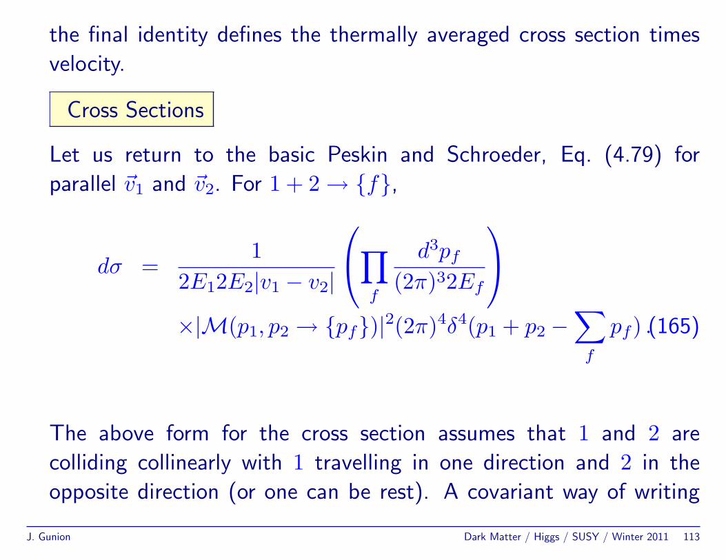
the final identity defines the thermally averaged cross section times

velocity.

Cross Sections

Let us return to the basic Peskin and Schroeder, Eq. (4.79) for

parallel ~v1 and ~v2. For 1 + 2 → f,

dσ =1

2E12E2|v1 − v2|

∏f

d3pf(2π)32Ef

×|M(p1, p2 → pf)|2(2π)4δ4(p1 + p2 −

∑f

pf) .(165)

The above form for the cross section assumes that 1 and 2 are

colliding collinearly with 1 travelling in one direction and 2 in the

opposite direction (or one can be rest). A covariant way of writing


this prefactor is to use

2E12E2|v1 − v2| = 4√

(p1 · p2)2 −m21m

22 . (166)

In a non-collinear situation√(p1 · p2)2 −m2

1m22

E1E2≡ |vMol| =

[|~v1 − ~v2|2 − |~v1 × ~v2|2

]1/2,

(167)

where vMol is called the Moller velocity. Sometimes, the distinction

between |v1 − v2| and |vMol| is ignored in the literature, at least

for pedagogical purposes (e.g. in Kolb and Turner). Since dσ is

a relativistic covariant (by the way it is defined), one should use

the relativistically covariant form of the prefactor. After all, in the

process of thermal averaging not all momenta of the colliding dark

matter particles are collinear. And, one does find that this difference

is important numerically in some cases.


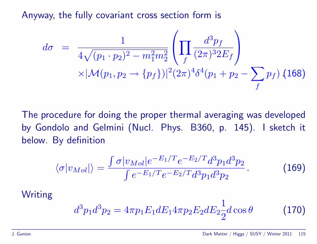
Anyway, the fully covariant cross section form is

dσ =1

4√

(p1 · p2)2 −m21m

22

∏f

d3pf(2π)32Ef

×|M(p1, p2 → pf)|2(2π)4δ4(p1 + p2 −

∑f

pf) .(168)

The procedure for doing the proper thermal averaging was developed

by Gondolo and Gelmini (Nucl. Phys. B360, p. 145). I sketch it

below. By definition

〈σ|vMol|〉 =∫σ|vMol|e−E1/Te−E2/Td3p1d

3p2∫e−E1/Te−E2/Td3p1d3p2

. (169)

Writing

d3p1d3p2 = 4πp1E1dE14πp2E2dE2

12d cos θ (170)


and then changing variables to (for simplicity, assume m1 = m2 = m)

E+ = E1 +E2 , E− = E1−E2 , s = 2m2 +2E1E2− 2p1p2 cos θ(171)

yields

d3p1d3p2 = 4π2E1E2dE+dE−ds . (172)

In terms of these new variables, the integration region (E1 > m,E2 >

m, | cos θ| ≤ 1) transforms into

|E−| ≤√

1− 4m2

s

√E2

+ − s , E+ ≥√s , s ≥ 4m2 , (173)

and

|vMol|E1E2 =√

(p1 · p2)2 −m4 =12

√s(s− 4m2) . (174)


is a function of s only. The numerator is then computed as∫σ|vMol|e−E1/Te−E2/Td3p1d

3p2

= 2π2

∫dE+

∫dE−

∫dsσ|vMol|E1E2e

−E+/T

= 4π2

∫ ∞

4m2dsσ

12

√s(s− 4m2)

√1− 4m2

s

∫ ∞

√s

dE+e−E+/T

√E2

+ − s

= 2π2T

∫ ∞

4m2dsσ(s− 4m2)

√sK1(

√s/T ) . (175)

Meanwhile, the denominator is∫e−E1/Td3p1

∫e−E2/Td3p2 =

[4πm2TK2(m/T )

]2. (176)

The Ki are the modified Bessel functions of order i.

Of course, the cross section itself has a prefactor proportional to

1/|vMol| so that σ|vMol| will behave like |M(p1, p2 → pf)|2. For


example, in the 1 + 2 → 3 + 4 case, we have

dσ

dt=

164πs

1p21 cm

|M|2 (177)

where s = (p1 + p2)2 and t = (p1 − p3)2 are the usual Mandelstam

invariants. In the cm frame, one can write

dt = −2p1 cmp3 cmd cos θcm (178)

so that

dσ

dΩcm=

164π2s

p3 cm

p1 cm|M|2 =

164π2s

βcmfβ cmi

|M|2 , (179)

where

βf =[1− (m3 +m4)2/s

]1/2 [1− (m3 −m4)2/s

]1/2(180)

βi =[1− (m1 +m2)2/s

]1/2 [1− (m1 −m2)2/s

]1/2, (181)


the latter reducing to βi =√

1− 4m2/s for m1 = m2 = m, are

entirely expressed in terms of the relativistic invariant s, as will be

|M|2. Using the m1 = m2 = m form of βi, Eq. (175) reduces to∫σ|vMol|e−E1/Te−E2/Td3p1d

3p2

= 2π2T

∫ ∞

4m2ds

164π2s

βf

∫dΩcm|M|2s

√s− 4m2K1(

√s/T )

(182)

Ultimately, what will be really important is the behavior of |M|2.In the absence of a Sommerfeld enhancement effect (which could

introduce an extra 1/|vMol|)2 it will behave as |vMol|p, with p = 0for S-wave annihilation, p = 2 for P-wave annihilation, and so forth.

2For example, Sommerfeld enhancement can arise from the exchange of a very light gauge boson in the t-channelbetween the dark matter particles prior to their annihilation.


So, now let us consider a particular case.

χ+ χ↔ B +B

Referring back to Eq. (164) we have in the initial state 1 = χ and

2 = χ and in the final state 3 = B and 4 = B. At this point we

then have a Boltzmann equation that reads (using v ≡ |vχχMol| and

assuming nχ = nχ)

nχ + 3Hnχ = −〈σχχ→BB|v|〉[n2χ − (neqχ )2] , (183)

Before proceeding further, as an aside let me sketch a simpler

treatment. We could have said that physically

nχ + 3Hnχ = −R(χχ→ BB)nχnχ +R(BB → χχ)nBnB . (184)

where the R’s are appropriate rate factors.


In equilibrium, the rhs must be zero to have no net change in particle

numbers, implying that

R(χχ→ BB)neqχ neqχ = R(BB → χχ)neqB n

eq

B. (185)

This relation is called detailed balance. It gives the same net effect as

the energy conservation plus time reversal gave in the more detailed

approach above.

We then appeal to the physical argument that R(χχ→ BB) would

have to be given (dimensionally at any rate) by 〈σχχ→BB|v|〉.

Anyway, let us now continue with the development of the formalism.

The structure developed above generalizes in a very natural way toχ + A → F where A and F are systems of particles. The generalBoltzmann equation for this case looks like:

nχ + 3Hnχ = −ZdΠχdΠAdΠF |M|2χ+A→F (2π)

4δ

4(pχ + pA− pF )[fχfA− fF ] , (186)


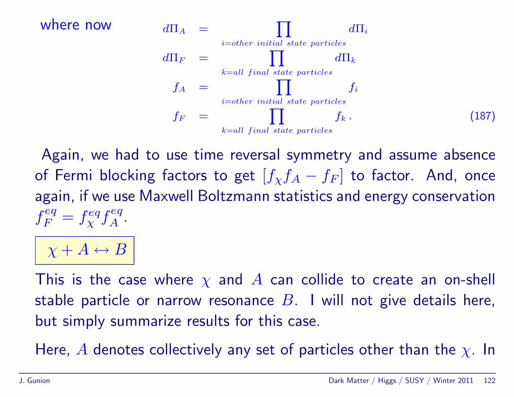
where now dΠA =Y

i=other initial state particles

dΠi

dΠF =Y

k=all final state particles

dΠk

fA =Y

i=other initial state particles

fi

fF =Y

k=all final state particles

fk . (187)

Again, we had to use time reversal symmetry and assume absence

of Fermi blocking factors to get [fχfA − fF ] to factor. And, once

again, if we use Maxwell Boltzmann statistics and energy conservation

feqF = feqχ feqA .

χ+A↔ B

This is the case where χ and A can collide to create an on-shell

stable particle or narrow resonance B. I will not give details here,

but simply summarize results for this case.

Here, A denotes collectively any set of particles other than the χ. In


this case we have

nχ + 3Hnχ = −R(χA→ B)nχnA +R(B → χA)nB (188)

where the R(. . .) are forward and backward rate coefficients. For the

first term, if A is a single particle (the usual case) R = 〈σχ+A→B|v|〉.The second term only depends on the number of B particles around

and Γ(B → χA) is the spontaneous decay rate.

Again, we have assumed occupation numbers are low (e.g. all massive

particles), so that there are no fermi blocking or bose enhancement

effects. In this approximation, the rate of producing B is independent

of the existing nB.

Again, we see from the above equation that for Γ H the collision

term is small compared to the Hubble expansion term, which means

that the system will go out of equilibrium.

• Calculation of the relic abundance:


Let us consider further the important case of χ+χ↔ B+B, where

B is a single particle, but where in general we must sum over all B’s.

For any species of particles which is not being created or destroyed,

n ∝ R−3, and we can assign a conserved number Y ∝ nR3. Since

s ∝ R−3, we can define this number to be

Y ≡ n/s . (189)

Scaling of entropy

We will be discussing the decoupling of χ from other species that

remain in equilibrium. Above, we made the statement that entropy

scales like R−3. This assumes the preceding statement that so long

as a species of particle is not being created or destroyed, it is included

in n ∝ R−3 and will be counted in the entropy.

The DM annihilation will simply shut off and will not heat up the


photons and other things that remain in thermal equilibrium.

The effective g∗S for the things that remain in equilibrium willdrop, but the entropy WILL NOT drop. One must continue to count

in the DM objects that are still present (they did not annihilate away).

The point is that there is still simply the combinatorial entropy of

the ”heavy billiard balls” that the DM is. It is given by the number

density of DM particles, i.e. their energy density divided by their

mass — if you like, one bit per particle, roughly.

The combinatorial entropy from the DM particles still scales as 1/Rand so it seems to scale as T . And, it is normalized to gDMT

3

because this is what it was BEFORE decoupling.

In other words, both before and after the DM has decoupled it is

correct to write

g∗S = gnon−DM equilibrium stuff∗S + gDM∗S , . (190)


This total g∗S does not change — s remains continuous. It does not

jump, as it cannot thanks to the 2nd law of thermodynamics.

You just wouldn’t use the standard relativistic formulas to calculate

the entropy.

This can be compared to, for instance, supersymmetric particles.

These do not simply decouple. When one crosses below their

threshold, they actually annihilate to less massive particles and one

really does not continue to count them — g∗S does decrease, but

the entropy is conserved because the temperature does increase due

to the annihilation feeding into the lower mass particles.

In summary, during decoupling vs. annihilation s stays smooth.

And, when you calculate it, you can use the standard relativistic

formulas for all things as computed when they were in equilibrium at

HIGH T >> all masses, and the evolution takes care of the rest.

Of course, it is important that the DM particles be included in


computing the total g∗S when performing computations.

For example, if the χ is quite heavy and all the SM particles are still

around (T > 300 GeV) and in addition we have χ, χ, one needs to

modify the old formula of Eq. (517) that gave g∗S = g∗ = 106.75by adding in (7/8)2× 2 (2 spins, 2 for particle plus antiparticle, 7/8being present if we assume the χ is a fermion).3

Taking this kind of modification into account, we can now proceed

using the standard scaling laws.

In thermal equilibrium, for a relativistic species χ (mχ T, µχ T )

we have

Yχ =452π4

ζ(3)gχg∗S

, (191)

3In supersymmetry, the χ is its own antiparticle so the 2nd factor of 2 is not present. Also, in supersymmetry, it isassumed that the χ is the lightest supersymmetry partner, so that all other superparticles would have annihilated by thetime T reaches the value at which the χ decouples.


whereas for a non-relativistic species (mχ T ) we have

Yχ =45

4√

2π7

gχg∗S

(mχ

T

)3/2

exp [−(mχ − µχ)/T ] . (192)

Here, T is generally dominated by the relativistic species, as they

contribute by far the biggest part to the entropy. At this point it is

useful to remind ourselves that TCMB ∼ 2.35× 10−4 eV.

If the species χ is stable, then the dominant process which can change

the number of particles in a comoving volume are the annihilation

and inverse annihilation processes χ+ χ↔ B +B.

Assuming, as before, that there is no asymmetry between particles

and antiparticles, and that B and B remain in thermal equilibrium

throughout the freeze out of the χ’s we have

nχ = nχ , nB = nB = neqB . (193)


To reemphasize, the idea behind the B,B remaining in equilibrium

is that the particles B,B will usually have additional interactions

(beyond those with χ, χ) which are “stronger” than their interactions

with the χ’s, so that they will remain in equilibrium even as the

χ’s fall out of equilibrium. An example would be χ, χ = ν, ν and

B,B = e−, e+; the neutrinos only have weak interactions whereas

the e±’s have weak and electromagnetic interactions.

Inputting Eq. (193) and the detailed balance relation of Eq. (185)

into Eq. (184) we obtain

nχ + 3Hnχ = −R(χχ→ BB)[n2χ − (neqχ )2

], (194)

where the annihilation rate R(χχ → BB) = 〈σχχ→BB|v|〉. After

summing over all possible B’s we obtain 〈σχ|v|〉, where σχ is the

total annihilation cross section and |v| = |vχχMol|. The 〈. . .〉 indicates

thermal averaging as defined in Eq. (164).


We now note that for Yχ ≡ nχ/s we find (using s ∝ T 3 withT ∝ 1/R so that s = KR−3 for some constant K — see earlierdiscussion which discussed why the scaling of s does not changeduring decoupling)

Yχ =nχs− nχ

s

s2=nχs− nχ

−3KR−4R

K2R−6

=nχs

+ 3nχR2R

K=nχs

+ 3nχ

(R

R

)(R3

K

)=nχs

+3nχHs

. (195)

which in turn implies that

sYχ = nχ + 3Hnχ. (196)

This is the reason why normalization of nχ to s is useful.

To proceed further, we introduce the dimensionless parameter x ≡mχ/T which will replace our time variable through the fact that

T = T (t). During the radiation dominated epoch, x and t are related


by [c.f. Eq. (99)]

t ' 0.301g−1/2∗ MP/T

2 = 0.301g−1/2∗

MP

m2x2 . (197)

Now, using the fact that T = KR , where K is some constant (not the

same as that used above), and defining Y ′χ ≡dYχdx we find

Yχ =dx

dtY ′χ =

dx

dT

dT

dtY ′χ =

[−mχ

T 2

][−KRR2

]Y ′χ =

[−mχ

R2

K2

][−KRR2

]Y ′χ

= mχR

KY ′χ =

mχ

T

TR

KY ′χ = x

R

RY ′χ = xHY ′χ . (198)

Using this, the Boltzmann equation becomes

Y ′χ = −〈σχ|v|〉s

Hx

[Y 2χ − (Y eqχ )2

]. (199)


If we now multiply by x/Y eqχ we obtain (using s = seq =neqχYeqχ

)

x

Y eqχY ′χ = −〈σχ|v|〉

neqχY eqχ

1HY eqχ

[Y 2χ − (Y eqχ )2

]= −Γχ

H

[(YχY eqχ

)2

− 1

],

(200)

where we have defined Γχ ≡ nχ〈σχ|v|〉.

Clearly, Γχ/H describes the “efficiency” of the annihilations relative

to the Hubble expansion when in equilibrium. The rate at which the

number of χ’s per comoving volume changes is controlled by this

efficiency factor times a measure of the deviation from equilibrium.

1. When Γχ H, the interactions are fast enough that the χ’s

thermalize and Yχ→ Y eqχ .

2. When Γχ H, the rhs “turns off” and Y ′χ = 0, implying that

the abundance Yχ “freezes in” to the value Y eqχ (xf), where xf =mχ/Tf with Tf being the “freeze out” temperature.


The equilibrium form of Yχ is different in the case where χ is still

relativistic at the time of freeze out vs. that when the χ is non-

relativistic at the time of freeze out. One finds from Eqs. (191) and

(192), respectively

Y eqχ = 0.278gχ

g∗S(x)if x 1 (201)

Y eqχ = 0.145gχ

g∗S(x)x3/2e−x if x 1 . (202)

In the above, gχ is the value for the number density, nχ, which for

fermions is the standard counting factor times 3/4 and for bosons is

simply equal to the standard counting factor. As noted earlier,

g∗S = gnon−DM particles remaining in eq∗ + gχ does not actually

change during the decoupling process.

We now consider these two cases in a bit more detail.


Hot relics

If the species decouples when still relativistic, say xf = mχ/Tf < 3,

then at that time Y eqχ is constant in time and the final, asymptotic

value of Yχ is quite insensitive to the details of freeze out (i.e. the

precise value of xf and precise behavior of 〈σχ|v|〉): from Eq. (201)

Y∞ ≡ Yχ(x→∞) ∼ Y eq(xf) = 0.278gχ

g∗S(xf). (203)

That is, the species freezes out with order unity abundance relative

to s [which is roughly the number of photons — s = 1.8g∗Snγ, see

Eq. (119)].

If we assume that there is no further entropy production following

the decoupling of the χ’s (i.e. no actual annihilations), then both s


and nχ will behave as 1/R3 and the abundance of χ’s today is

n0χ = s0Y∞ ' 2905Y∞ cm−3 = 808

[gχ

g∗S(xf)

]cm−3 , (204)

where 2905 comes from the Table of Eq. (139).

If, after freeze out, the entropy per comoving volume of the Universe

should increase, say by a factor of γ (presumably due to some

annihilations), then the present abundance of χ’s in a comoving

volume would be diminished by γ: Y∞ = Y (xf)/γ.A species that decouples when it is relativistic is often called a “hotrelic”. The present relic mass density contributed by a (once) hot(but now cold, mχ T0) relic of mass mχ is simply

ρ0χ = n0

χmχ = 808[

gχg∗S(xf)

]cm−3

(mχ

eV

)eV (205)

Ω0χh

20 =

ρ0χ

ρ0c

= 7.65× 10−2

[gχ

g∗S(xf)

](mχ

eV

), (206)


where we recall that H0 = 100h0 km sec−1 Mpc−1 ' h09.25×1027cm

,

so that

ρ0c =

3H20

8πG= h2

0 1.057× 104 eVcm3

. (207)

where I used G in the form

G = 6.71×10−39

GeV−2

= 6.71×10−39

GeV−1

0.197× 10−13

cm = 1.32×10−61 eV

cm.

(208)

We know that for sure Ω0h20<∼ 1 at the present day. Combined

with the above value for Ω0χh

20, we conclude that

mχ <∼ 13 eV[g∗S(xf)gχ

]. (209)

Light mass (mχ <∼ MeV) neutrinos decouple when T ∼ few×MeVat which point g∗S = g∗ = 10.75, not including the χ, χ, but this

does include our SM neutrinos. For a single, extra 2-component

neutrino species (plus anti-neutrino) we have gχ = (3/4)× 2 = 1.5,


so that gχ/g∗S(xf) = 0.122 if we include g∗ S χ = (7/8)gχ in g∗S.

KT, however, focus on applying this game to the SM neutrinos that

are already included in g∗S = 10.75. In this case, the appropriate

factor isgχg∗S

= 1.510.75 ∼ 0.140. Plugging this in, we find that

Ω0ννh

20 ∼

mν

93.5 eV, mν <∼ 93.5 eV . (210)

Of course, we actually have stronger constraints on Ω0ννh

20, coming

from all the other things that we know contribute to Ω0h20 such as

cold dark matter. Looking back at earlier tabulations we learn that

Ω0m ' 0.136 while Ω0

cdm ' 0.113. This leaves room for Ω0hdm ∼

0.023. Now multiplying by h20 ∼ (0.7)2 gives Ω0

hdmh20 < 0.0115.

So, very roughly we now know that

Ω0ννh

20<∼ 0.01 (211)


resulting in a bound of

mν <∼ 0.935 eV (212)

on any single neutrino. If there are also axions, then this bound is

strengthened. However, we also know that the 3 neutrinos are pretty

degenerate, yielding

mν < 0.31 eV (213)

for each. This is the bound that is relevant for the current data.

If the overall Ω0ννh

20<∼ 0.01 bound decreases with future data, one

could arrive at a situation where the lightest neutralino would have

to be nearly massless given the measured ∆m2 between neutrinos.

The point at which this happens depends upon whether the neutrinos

have a normal hierarchy with m3 > m2 >∼ m1 (1 = e, 2 = µ, 3 = τ)

or inverted hierarchy with m2 >∼ m1 > m3. The key input is

the measured value of ∆m232 ∼ 2.43 × 10−3 eV2. Recall also that


∆m212 ∼ 7.6× 10−5 eV2 is much smaller.

1. In the normal hierarchy case, m2 ∼ m1 ∼ 0, the measured ∆m223

would yield m3 ∼ 0.049 eV. Since 1 and 2 are much lighter than

3, this is a single “heavy” neutrino case. It could be tested by

cosmological data if Ω0ννh

20<∼ 0.0005 could be probed.

2. In the inverted hierarchy case, at the limit m3 ∼ 0 one would have

m2 ∼ m1 ∼ 0.049 eV, i.e. two “heavy” neutrinos, which could be

tested if Ω0ννh

20<∼ 0.001 could be probed.

In either case, LSST is potentially capable of obtaining the required

precision on Ω0ννh

20, but I don’t believe it will be reached by

experiments planned between now and then.

Of course, we can also consider a ψ that decouples much earlier on,

in particular when T >∼ 300 GeV (requiring that the ψ interact

even more weakly than a neutrino). Let us assume that the ψ has

gψ = 1.5. Then g∗S(xf) ' g∗(xf) ∼ 106.75 + (7/8)× 1.5 ∼ 108.06


and gψ/g∗S ' 1.5/108.06 ' 0.0139. Then, the present contribution

to the energy density is very roughly

Ω0ψψh2

0 =mψ

910 eV, (214)

which is about a factor of 10 less than that of a conventional neutrino

species of the same mass.

The present number density of such a species is given by the standard

formula, see Eq. (204),

n0ψ ∼ 808

[gψ

g∗S(xf)

]cm−3 ∼ 11 cm−3 , (215)

so that n0ψ n0

γ ∼ 413 cm−3.

Thus, a species that decouples when g∗S 1 has a present

abundance that is much less than that of the microwave photons, and

if the species is massless, a temperature much less than the photon


temperature, Tψ ' (3.91/g∗S(xf))1/3T . For the latter reason, such

a relic is often referred to as warm relic.

In this case, the temperatures for the ψ and for the photons, T = Tγ,

diverge precisely because a lot of the SM particles do in fact annihilate

and feed entropy into the photons. Entropy conservation requires

that T = Tγ increases when annihilations occur and g∗S decreases.

Examples of such a warm relic include a light gravitino, or a light

photino, where light means mψ <∼ keV.


Cold relics

The definition of “cold” is that freeze out occurs when the species is

non-relativistic (xf >∼ 3).

This is a more difficult case than the hot relic case. At the time of

freeze out Y eq is decreasing exponentially with x. As a result the

precise details of freeze out are important.

Gondolo and Gelmini proceed by expanding

σχ|vMol| =∞∑n=0

ann!εn , (216)

where

ε =s− 4m2

χ

4m2χ

(217)

is the kinetic energy per unit mass in the laboratory frame. For s


close to threshold, s ∼ 4m2χ, ε ∼ (βc.m.i )2, but it is more correct to

define it as above.

They then use the formulas given earlier to show that

〈σχ|vMol|〉 = a0 +32a1x

−1 +[92a1 +

158a2

]x−2 + . . . , (218)

where, as before, x = mχ/T . They note that this compares to

the non-relativistic approximation implicit in Kolb and Turner, which

gives

〈σχ|vMol|〉n.r. = a0 +32a1x

−1 +158a2x

−2 + . . . . (219)

The expressions only begin to differ at order x−2. In the non-

relativistic limit, one can think of σχ|vMol| ∝ |vMol|p, where p = 0, 2corresponds to S-wave, P-wave annihilation.


Since 〈|vMol|〉 ∝ T 1/2, 〈σχ|vMol|〉 ∝ Tn, with n = 0, 1 for S-wave,

P-wave annihilation, respectively.

In any case, regardless of whether we use the full relativistic treatment

with vMol or the non-relativistic treatment, we may write (as in KT)

〈σχ|v|〉 ≡ σ0(T/mχ)n = σ0x−n , for x >∼ 3 . (220)

Meanwhile, we should recall that s ∝ T 3 ∝ x−3 and H = RR ∝ t−1 ∝

x−2 [c.f. Eq. (197)]. Using the above parameterization for 〈σχ|v|〉and these scalings, the Boltzmann equation, Eq. (199),

Y ′χ = −〈σχ|v|〉s

Hx

[Y 2χ − (Y eqχ )2

], (221)

can be rewritten in the form

dYχdx

= −λx−(n+2)[Y 2χ −

(Y eqχ

)2], (222)


where

λ =[〈σχ|v|〉sxH(x)

]x=1

Eqs. (116,98)= 0.264(g∗S/g1/2

∗ (x))MPmχσ0 (223)

Y eqχEq. (202)

= 0.145(gχ/g∗S(x))x3/2e−x . (224)

The first two equations referenced above were

s =2π2

45g∗ST

3

and

H =[8πG

3π2

30g∗T

4

]1/2= 1.66g1/2

∗T 2

MP,

while Eq. (202) came from the earlier expression of Eq. (192), namely


for non-relativistic particles

Yχ =45

4√

2π7

gχg∗S

(mχ

T

)3/2

exp [−(mχ − µχ)/T ] .

and we have taken T = mχ (x = 1) for the computation of s and H

for getting λ.

To be absolutely clear, 〈σA|v|〉 sxH as a function of x takes the form

〈σA|v|〉 sxH

=σ0 x

−n(

2π2

45 g? Sm3χ

x3

)x(8πG

3

)1/2g1/2?

m2χ

x2

= mχ2π2

45

(3

8πG

)−1/2g? S

g1/2?

σ0︸︷︷︸λ

x−(n+2)

≡ λx−(n+2) . (225)


Note that because of the MP factor in λ, λ 1.

We are now ready to solve the Boltzmann equation using some

approximate techniques.

Define ∆ = Y − Y eq. We then have from Eq. (222)

∆′ = −Y eq′ − λx−(n+2)∆(2Y eq + ∆) , (226)

where (assuming constant g∗S during decoupling) Eq. (224) implies

Y eq′ = Y eq(

32x− 1)' −Y eq , (227)

if the relevant x values are large, as will turn out to be the case.

With this approximation for Y eq′, Eq. (226) takes the form

∆′ = Y eq − λx−(n+2)∆(2Y eq + ∆) , (228)


At early times (1 < x xf), Y tracks Y eq very closely, and both ∆and |∆′| are small. So an approximate solution is obtained by setting

∆′ = 0, yielding

∆ ' λ−1xn+2Y eq/(2Y eq + ∆) (229)

' 12λxn+2 . (230)

At late times (x xf), Y tracks Y eq very poorly: ∆ ' Y Y eq,

and the terms in Eq. (226) involving Y eq′ and Y eq can be safely

neglected, so that

∆′ = −λx−(n+2)∆2 .⇒ d∆∆2

= −dx λ

x(n+2). (231)

Upon integration of this latter equation from x = xf to x = ∞, we


obtain1

∆∞− 1

∆(xf)=

λ

(n+ 1)xn+1f

. (232)

It remains to determine xf .

We recall that x = xf is the time when Y ceases to track Y eq, or

equivalently, when ∆ becomes of order Y eq. Let us define xf by the

criterion ∆(xf) = cY eq(xf), where c is a numerical constant of order

unity. Substituting this into Eq. (229) evaluated at x = xf yields

∆(xf) 'xn+2f

λ(2 + c). (233)

Using ∆(xf) = cY eq(xf) = cax3/2f e−xf with a = 0.145(gχ/g∗S),

see Eq. (224), we have the freeze out condition

cax3/2f e−xf =

xn+2f

λ(2 + c), (234)


which has the approximate solution

xf ' ln[(2 + c)λac]−(n+

12

)lnln[(2 + c)λac] . (235)

Note that xf depends only logarithmically upon the numerical

condition for freeze out, i.e. the value of c, as will the final abundance

— see below.

Meanwhile, plugging ∆(xf) 'xn+2f

λ(2+c) into Eq. (232) yields an

expression for 1∆∞

:

1∆∞

=λ(2 + c)xn+2f

+λ

(n+ 1)xn+1f

. (236)

Assuming xf will turn out to be large we may drop the first term and

obtain

Y∞ ' ∆∞ ' n+ 1λ

xn+1f , (237)


where we have used Y eq∞ ∝ e−∞ = 0 so that ∆∞ = Y∞−Y eq∞ = Y∞.

Figure 4: Freeze-out plots from Kolb and Turner and from Bergstrom and Goobar.This latter seems to have correction normalization label.

One can of course perform a numerical integration of the Boltzmann

equation with the result shown. Choosing c(c + 2) = n + 1 gives

the best fit to the numerical results for the final abundance Y∞ (to


better than 5% for any xf ≥ 3).

With the above choice of c our formula for xf simplifies to

xf = ln[λa]−(n+

12

)ln ln[λa]

= ln[0.038(n+ 1)(gχ/g1/2

∗ )MPmχσ0

]−(n+

12

)ln

ln[0.038(n+ 1)(gχ/g1/2

∗ )MPmχσ0

],

(238)

where 0.038 = 0.264 × 0.145 comes from the coefficients in λ and

a, Eqs. (223) and (224), respectively. Note the big MP in the xfexpression which means that xf will typically be big unless σ0 is really

tiny (in appropriate inverse mass-squared units).

Using Eq. (237) and keeping only the first term in the xf expression


above, gives

Y∞ =3.79(n+ 1)xn+1

f

(g∗S/g1/2∗ )MPmχσ0

(239)

Just as for hot relics, we use

n0χ = s0Y∞ = 2905Y∞ cm−3 (240)

but with the above expression for Y∞, yielding

n0χ = 1.101× 104

(n+ 1)xn+1f

(g∗S/g1/2∗ )MPmχσ0

(241)

with corresponding results of

ρ0χ = n0

χmχ = 1.101× 104(n+ 1)xn+1

f

(g∗S/g1/2∗ )MPσ0


Ω0χh

20 =

(ρ0χ

ρ0c

)h2

0 = 1.042× 109(n+ 1)xn+1

f GeV−1

(g∗S/g1/2∗ )MPσ0

(242)

where in this case we wrote ρ0c in GeV units (c.f. Eq. (207)):

ρ0c =

3H20

8πG= h2

0 1.057× 10−5 GeVcm3

. (243)

Obviously, xf and the final Ω0χh

20 depend on σ0. A few examples are

in order.

Heavy (m MeV), stable neutrino species

Because of its large mass, such a neutrino, call it N , will decouple

when it is non-relativistic (to be verified) and the formulae for a cold

relic apply.

Annihilation for such a species proceeds through Z exchange to final

states ii with i = νL, e, µ, τ, u, d, s, . . . The annihilation cross section


depends upon whether the N is of the Dirac or Majorana type. For

T <∼ mN <∼ mZ, we find

〈σN |v|〉Dirac =G2Fm

2N

2π

∑i

(1− z2i )

1/2

×[(C2Vi

+ C2Ai

)(1 +

12z2i

)](244)

〈σN |v|〉Maj =G2Fm

2N

2π

∑i

(1− z2i )

1/2

×[(C2Vi

+ C2Ai

) 8β2i

3+ C2

Ai2z2i

], (245)

where zi ≡ mi/mN , β is the relative velocity in the cm, and CV and

CA are given in terms of the weak isospin I3, the electric charge q

and the Weinberg angle θW by CA = I3, CV = I3−2q sin2 θW . The

sum ranges over all quark and lepton species lighter than mN .44We are assuming that mN < mZ and are therefore using the “contact” Fermi 4-point style of interaction, equivalent

to the approximation 1/[(s−m2Z)2 + Γ2

Z/4] ∼ 1/m4Z .


Focusing on the Dirac case, annihilations proceed through the S-wave

and 〈σN |v|〉 is velocity independent:

σ0 ' c2G2Fm

2N

2π, (246)

where c2 ∼ 5 after performing the sums. Taking gN = 2 (2 spins but

no 2nd 2 for N since Boltzmann focuses on only N , or N , on its

own) and g∗ ∼ 60 (no W,Z, t, b,H ⇒ 106.75 − 31 = 75.75?), from

our formulae for xf and Y∞ we find

xf ' 15 + 3 ln(mN/ GeV) + ln(c2/5)

Y∞ ' 6× 10−9( mN

GeV

)−3[1 +

3 ln(mN/ GeV)15

+ln(c2/t)

15

](247)


from which we obtain

Ω0NN

h20 ' 3

( mN

GeV

)−2[1 +

3 ln(mN/ GeV)15

], (248)

where we included the factor of 2 for N +N abundance.

We observe that freeze out takes place at

Tf ' mN/15 ' 70 MeV(mN/ GeV) , (249)

which, in particular, is before the light neutrinos freeze out. The heavy

neutrinos annihilate and become rare early on, and the annihilaton

process quenches.

If we require that the N,N not overclose the Universe, Ω0NN

h20 ≤ 1,

we obtain the “Lee-Weinberg” bound of

mN >∼ 2 GeV . (250)


Of course, nowadays we might ask that the N (which in the mass

range being considered should be non-relativistic) should give the

observed (mainly cold) dark matter density: Ω0NN

h20 ∼ 0.11. This

would work for mN ∼√

30 GeV.

The problem is that since the N that we are envisioning couples to

the Z, it would have appeared at LEP in Z decays. LEP excludes such

a heavy neutrino for mN < mZ/2 ∼ 45 GeV; for mN > 45 GeV,

Ω0NN

h20 < 0.0015.

For the Majorana case, annihilation proceeds through both the S-

wave and the P-wave. However, the formulae for xf , Y∞ and Ω0NN

h20

are similar. The plot below gives a comparison of the two cases.


We note:

– For mN <∼ MeV, Ω0NN

h20 ∝ mN because the relic abundance is

constant.

– For mN >∼ MeV, Ω0NN

h20 ∝ m−2

N due to the fact that the relic

abundance is decreasing like m−3N .

– Ω0NN

h20 achieves its maximum for mN ∼ MeV.

– Requiring Ω0NN

h20<∼ 0.01 (which is beyond the plot limits) implies


mN <∼ 1 eV on the low side.

In this region, Z decay limits imply that there is no room for a new

N in addition to the standard 3 neutrino species.

– As mentioned above, on the high side mN >∼ 45 GeV is required

by LEP and extending the graph would show that Ω0NN

h20 ∼

0.0015(

45 GeVmN

)2

in the Dirac case.

LSP of MSSM

For this, we need to make an excursion into supersymmetry. However,

from the previous discussion, we already see that the LSP cannot be

that closely analogous to a heavy N if it is to supply the observed

cold dark matter.

This is because a heavy-neutrino N does not give enough dark matter.

What seems to be required is that the 〈σχ|v|〉 be substantially smaller

than that for a recurrence of a neutrino with SM-like couplings.


This can be accomplished in the context of supersymmetry provided

the χ LSP has the correct composition in terms of its bino, wino,

and higgsino (and in the NMSSM, singlino) content.

This shows the limitation of the WIMP miracle argument. We are

quite sensitive to the actual cross section and so the WIMP miracle

in the Ω0DMh

20 sense is only a miracle within a factor of 100 or so,

which is already quite an achievement, but more precision is needed.

So, at this point, a we must learn more about Supersymmetry.


Supersymmetry

As I mentioned at the beginning of the quarter, I will not be deriving

the rules for constructing a supersymmetric Lagrangian, I will simply

state those rules and give the procedures for employing such a

Lagrangian. I will be following Steve Martin’s “Supersymmetry

Primer” for notation since that is easily available on the arXiv.

Other possible references include the old Haber-Kane Physics Report,

John Ternings “Modern Supersymmetry”, and the Wess-Bagger

“Supersymmetry and Supergravity”. For detailed Feynman rule

derivations and spinor techniques, see Dreiner, Haber and Martin,

arXiv:0812.1594. The 246 Supersymmetry Barcelona lecture attachment

on my home page focuses on the phenomenology of supersymmetry

at colliders. Although it is a bit old now, the general phenomenology

reviewed there is mostly still relevant.


General Structure of a Supersymmetric Theory

The extension of the Lorentz group to supersymmetry requires (see

Martin) an equal number of bosons and fermions:

nB = nF . (251)

The simplest possibility for a supermultiplet consistent with Eq. (251)

has a single Weyl fermion (with two spin helicity states, so nF = 2)

and two real scalars (each with nB = 1). It is natural to assemble

the two real scalar degrees of freedom into a complex scalar field;

as we will see below this provides for convenient formulations of

the supersymmetry algebra, Feynman rules, supersymmetry-violating

effects, etc. This combination of a two-component Weyl fermion

and a complex scalar field is called a chiral or matter or scalarsupermultiplet.


The next-simplest possibility for a supermultiplet contains a spin-1

vector boson. If the theory is to be renormalizable, this must be a

gauge boson that is massless, at least before the gauge symmetry is

spontaneously broken.

A massless spin-1 boson has two helicity states, so the number of

bosonic degrees of freedom is nB = 2. Its superpartner is therefore

a massless spin-1/2 Weyl fermion, again with two helicity states, so

nF = 2. (If one tried to use a massless spin-3/2 fermion instead, the

theory would not be renormalizable.)

Gauge bosons must transform as the adjoint representation of the

gauge group, so their fermionic partners, called gauginos, must

also. Since the adjoint representation of a gauge group is always

its own conjugate, the gaugino fermions must have the same

gauge transformation properties for left-handed and for right-handed

components. Such a combination of spin-1/2 gauginos and spin-1

gauge bosons is called a gauge or vector supermultiplet.


If we include gravity, then the spin-2 graviton (with 2 helicity states,

so nB = 2) has a spin-3/2 superpartner called the gravitino. The

gravitino would be massless if supersymmetry were unbroken, and so

it has nF = 2 helicity states.

There are other possible combinations of particles with spins that

can satisfy Eq. (251). However, these are always reducible to

combinations5 of chiral and gauge supermultiplets if they have

renormalizable interactions, except in certain theories with “extended”

supersymmetry.

The ordinary, non-extended, phenomenologically viable supersymmetric

model is sometimes called N = 1 supersymmetry, with N referring

to the number of supersymmetries (the number of distinct copies of

the generators Q,Q† of supersymmetry transformations).5For example, if a gauge symmetry were to spontaneously break without breaking supersymmetry, then a massless

vector supermultiplet would “eat” a chiral supermultiplet, resulting in a massive vector supermultiplet with physical degreesof freedom consisting of a massive vector (nB = 3), a massive Dirac fermion formed from the gaugino and the chiralfermion (nF = 4), and a real scalar (nB = 1).


Thus, In a supersymmetric extension of the Standard Model each

of the known fundamental particles is in either a chiral or gauge

supermultiplet, and must have a superpartner with spin differing by

1/2 unit.

The first step in understanding the exciting consequences of this

prediction is to decide exactly how the known particles fit into

supermultiplets, and to give them appropriate names.

Summary of the Chiral Supermultiplets

A crucial observation here is that only what are called chiral

supermultiplets can contain fermions whose left-handed parts transform

differently under the gauge group than their right-handed parts. All

of the Standard Model fermions (the known quarks and leptons) have

this property, so they must be members of chiral supermultiplets.6

6In particular, one cannot attempt to make a spin-1/2 neutrino be the superpartner of the spin-1 photon; the neutrinois in a doublet, and the photon is neutral, under weak isospin.


The names for the spin-0 partners of the quarks and leptons are

constructed by prepending an “s”, for scalar. So, generically they

are called squarks and sleptons (short for “scalar quark” and “scalar

lepton”), or sometimes sfermions.

The left-handed and right-handed pieces of the quarks and leptons

are separate two-component Weyl fermions with different gauge

transformation properties in the Standard Model, so each must have

its own complex scalar partner.

The symbols for the squarks and sleptons are the same as for

the corresponding fermion, but with a tilde (˜ ) used to denote

the superpartner of a Standard Model particle. For example, the

superpartners of the left-handed and right-handed parts of the

electron Dirac field are called left- and right-handed selectrons, and

are denoted eL and eR.

It is important to keep in mind that the “handedness” here does not


refer to the helicity of the selectrons (they are spin-0 particles) but

to that of their superpartners.

A similar nomenclature applies for smuons and staus: µL, µR, τL, τR.

The Standard Model neutrinos (neglecting their very small masses)

are always left-handed, so the sneutrinos are denoted generically by

ν, with a possible subscript indicating which lepton flavor they carry:

νe, νµ, ντ .

Finally, a complete list of the squarks is qL, qR with q = u, d, s, c, b, t.

The gauge interactions of each of these squark and slepton fields

are the same as for the corresponding Standard Model fermions; for

instance, the left-handed squarks uL and dL couple to the W boson,

while uR and dR do not.

It seems clear that the Higgs scalar boson must reside in a chiral

supermultiplet, since it has spin 0. Actually, it turns out that just

one chiral supermultiplet is not enough.


One reason for this is that if there were only one Higgs chiral

supermultiplet, the electroweak gauge symmetry would suffer a

gauge anomaly, and would be inconsistent as a quantum theory.

This is because the conditions for cancellation of gauge anomalies

include Tr[T 23Y ] = Tr[Y 3] = 0, where T3 and Y are the third

component of weak isospin and the weak hypercharge, respectively,

in a normalization where the ordinary electric charge isQEM = T3+Y .

The traces run over all of the left-handed Weyl fermionic degrees of

freedom in the theory.

In the Standard Model, these conditions are already satisfied, somewhat

miraculously, by the known quarks and leptons.

Now, a fermionic partner of a Higgs chiral supermultiplet must be a

weak isodoublet with weak hypercharge Y = 1/2 or Y = −1/2. In

either case alone, such a fermion will make a non-zero contribution

to the traces and spoil the anomaly cancellation. This can be avoided

if there are two Higgs supermultiplets, one Y = +1/2 and one with


Y = −1/2, so that the total contribution to the anomaly traces

from the two fermionic members of the Higgs chiral supermultiplets

vanishes by cancellation.

As we will see later, two Higgs chiral supermultiplets are also necessary

for another completely different reason: because of the structure of

supersymmetric theories, only a Y = 1/2 Higgs chiral supermultiplet

can have the Yukawa couplings necessary to give masses to charge

+2/3 up-type quarks (up, charm, top), and only a Y = −1/2 Higgs

can have the Yukawa couplings necessary to give masses to charge

−1/3 down-type quarks (down, strange, bottom) and to the charged

leptons.

We will call the SU(2)L-doublet complex scalar fields with Y = 1/2and Y = −1/2 by the names Hu and Hd, respectively.2

The weak isospin components of Hu with T3 = (1/2, −1/2) have2Other notations in the literature have H1, H2 or H,H instead of Hu, Hd. The notation used here has the virtue of

making it easy to remember which Higgs VEVs gives masses to which type of quarks.


electric charges 1, 0 respectively, and are denoted (H+u , H0

u).

Similarly, the SU(2)L-doublet complex scalar Hd has T3 = (1/2,

−1/2) components (H0d , H

−d ).

The neutral scalar that corresponds to the physical Standard Model

Higgs boson is in a linear combination of H0u and H0

d .

The generic nomenclature for a spin-1/2 superpartner is to append

“-ino” to the name of the Standard Model particle, so the fermionic

partners of the Higgs scalars are called higgsinos. They are denoted

by Hu, Hd for the SU(2)L-doublet left-handed Weyl spinor fields,

with weak isospin components H+u , H0

u and H0d , H

−d .

We have now found all of the chiral supermultiplets of a minimal

phenomenologically viable extension of the Standard Model. They

are summarized in Table 1, classified according to their transformation

properties under the Standard Model gauge group SU(3)C×SU(2)L×U(1)Y , which combines uL, dL and ν, eL degrees of freedom into


SU(2)L doublets.

Names spin 0 spin 1/2 SU(3)C, SU(2)L, U(1)Ysquarks, quarks Q (uL dL) (uL dL) ( 3, 2 , 1

6)(×3 families) u u∗R u†R ( 3, 1, −2

3)d d∗R d†R ( 3, 1, 1

3)sleptons, leptons L (ν eL) (ν eL) ( 1, 2 , −1

2)(×3 families) e e∗R e†R ( 1, 1, 1)

Higgs, higgsinos Hu (H+u H0

u) (H+u H0

u) ( 1, 2 , +12)

Hd (H0d H−

d ) (H0d H−

d ) ( 1, 2 , −12)

Table 1: Chiral supermultiplets in the Minimal Supersymmetric Standard Model. Thespin-0 fields are complex scalars, and the spin-1/2 fields are left-handed two-componentWeyl fermions.

Here we follow a standard convention, whereby all chiral supermultiplets

are defined in terms of left-handed Weyl spinors. In particular,

the conjugates of the right-handed quarks and leptons (and their

superpartners) appear in Table 1. This protocol for defining chiral


supermultiplets will prove very useful for constructing supersymmetric

Lagrangians.

It is also useful to have a symbol for each of the chiral supermultiplets

as a whole; these are indicated in the second column of Table 1. Thus,

for example, Q stands for the SU(2)L-doublet chiral supermultiplet

containing uL, uL (with weak isospin component T3 = 1/2), and

dL, dL (with T3 = −1/2), while u stands for the SU(2)L-singlet

supermultiplet containing u∗R, u†R.

There are three families for each of the quark and lepton supermultiplets,

Table 1 lists the first-family representatives. A family index i = 1, 2, 3can be affixed to the chiral supermultiplet names (Qi, ui, . . .) when

needed, for example (e1, e2, e3) = (e, µ, τ). The bar on u, d, e fields

is part of the name, and does not denote any kind of conjugation.

The Higgs chiral supermultiplet Hd (containing H0d , H

−d , H0

d , H−d )

has exactly the same Standard Model gauge quantum numbers as


the left-handed sleptons and leptons Li, for example (ν, eL, ν, eL).

Naively, one might therefore suppose that we could have been more

economical in our assignment by taking a neutrino and a Higgs

scalar to be superpartners, instead of putting them in separate

supermultiplets. This would amount to the proposal that the Higgs

boson and a sneutrino should be the same particle.

This attempt played a key role in some of the first attempts to connect

supersymmetry to phenomenology, but it is now known to not work.

Even ignoring the anomaly cancellation problem mentioned above,

many insoluble phenomenological problems would result, including

lepton-number non-conservation and a mass for at least one of the

neutrinos in gross violation of experimental bounds. Therefore, all of

the superpartners of Standard Model particles are really new particles,

and cannot be identified with some other Standard Model state.


The Vector Supermultiplets

The vector bosons of the Standard Model clearly must reside in

gauge supermultiplets. Their fermionic superpartners are generically

referred to as gauginos.

The SU(3)C color gauge interactions of QCD are mediated by the

gluon, whose spin-1/2 color-octet supersymmetric partner is the

gluino. As usual, a tilde is used to denote the supersymmetric

partner of a Standard Model state, so the symbols for the gluon and

gluino are g and g respectively.

The electroweak gauge symmetry SU(2)L × U(1)Y is associated

with spin-1 gauge bosons W+,W 0,W− and B0, with spin-1/2

superpartners W+, W 0, W− and B0, called winos and bino. After

electroweak symmetry breaking, the W 0, B0 gauge eigenstates mix

to give mass eigenstates Z0 and γ. The corresponding gaugino

mixtures of W 0 and B0 are called zino (Z0) and photino (γ); if


supersymmetry were unbroken, they would be mass eigenstates with

masses mZ and 0. Table 2 summarizes the gauge supermultiplets of

a minimal supersymmetric extension of the Standard Model.

Names spin 1/2 spin 1 SU(3)C, SU(2)L, U(1)Ygluino, gluon g g ( 8, 1 , 0)

winos, W bosons W± W 0 W± W 0 ( 1, 3 , 0)bino, B boson B0 B0 ( 1, 1 , 0)

Table 2: Gauge supermultiplets in the Minimal Supersymmetric Standard Model.

General Remarks on the MSSM and Supersymmetry Breaking

The chiral and gauge supermultiplets in Tables 1 and 2 make up

the particle content of the Minimal Supersymmetric Standard Model

(MSSM).

The most obvious and interesting feature of this theory is that

none of the superpartners of the Standard Model particles has been


discovered.

If supersymmetry were unbroken, then there would have to be

selectrons eL and eR with masses exactly equal to me = 0.511...MeV. A similar statement applies to each of the other sleptons

and squarks, and there would also have to be a massless gluino

and photino. These particles would have been extraordinarily easy

to detect long ago. Clearly, therefore, supersymmetry is a brokensymmetry in the vacuum state chosen by Nature.

An important clue as to the nature of supersymmetry breaking can

be obtained by returning to the motivation provided by the hierarchy

problem.

Supersymmetry forced us to introduce two complex scalar fields for

each Standard Model Dirac fermion, which is just what is needed to

enable a cancellation of the quadratically divergent (Λ2UV) one-loop

corrections to the Higgs mass. This sort of cancellation also requires


that the associated dimensionless couplings should be related (for

example λS = |λf |2).

The necessary relationships between couplings indeed occur in unbroken

supersymmetry. In fact, unbroken supersymmetry guarantees that

the quadratic divergences in scalar squared masses must vanish to all

orders in perturbation theory.3

Now, if broken supersymmetry is still to provide a solution to the

hierarchy problem even in the presence of supersymmetry breaking,

then the relationships between dimensionless couplings that hold in

an unbroken supersymmetric theory must be maintained. Otherwise,

there would be quadratically divergent radiative corrections to the

3A simple way to understand this is to recall that unbroken supersymmetry requires the degeneracy of scalar and fermionmasses. Radiative corrections to fermion masses are known to diverge at most logarithmically in any renormalizable fieldtheory, so the same must be true for scalar masses in unbroken supersymmetry.


Higgs scalar masses of the form

∆m2H =

18π2

(λS − |λf |2)Λ2UV + . . . . (252)

We are therefore led to consider “soft” supersymmetry breaking. This

means that the effective Lagrangian of the MSSM can be written in

the form

L = LSUSY + Lsoft, (253)

where LSUSY contains all of the gauge and Yukawa interactions and

preserves supersymmetry invariance, and Lsoft violates supersymmetry

but contains only mass terms and coupling parameters with positivemass dimension.

Without further justification, soft supersymmetry breaking might

seem like a rather arbitrary requirement. Fortunately, theoretical

models for supersymmetry breaking do indeed yield effective Lagrangians

with just such terms for Lsoft.


If the largest mass scale associated with the soft terms is denoted

msoft, then the additional non-supersymmetric corrections to the

Higgs scalar squared mass must vanish in the msoft → 0 limit, so by

dimensional analysis they cannot be proportional to Λ2UV.

More generally, these models maintain the cancellation of quadratically

divergent terms in the radiative corrections of all scalar masses, to

all orders in perturbation theory.

The corrections also cannot go like ∆m2H ∼ msoftΛUV, because in

general the loop momentum integrals always diverge either quadratically

or logarithmically, not linearly, as ΛUV →∞. So they must be of the

form

∆m2H = m2

soft

[λ

16π2ln(ΛUV/msoft) + . . .

]. (254)

Here λ is schematic for various dimensionless couplings, and the

ellipses stand both for terms that are independent of ΛUV and for

higher loop corrections (which depend on ΛUV through powers of


logarithms).

Because the mass splittings between the known Standard Model

particles and their superpartners are just determined by the parameters

msoft appearing in Lsoft, Eq. (254) tells us that the superpartner

masses cannot be too huge. Otherwise, we would lose our successful

cure for the hierarchy problem, since them2soft corrections to the Higgs

scalar squared mass parameter would be unnaturally large compared

to the square of the electroweak breaking scale of 174 GeV.

The top and bottom squarks and the winos and bino give especially

large contributions to ∆m2Hu

and ∆m2Hd

, but the gluino mass and all

the other squark and slepton masses also feed in indirectly, through

radiative corrections to the top and bottom squark masses.

Furthermore, in most viable models of supersymmetry breaking that

are not unduly contrived, the superpartner masses do not differ from

each other by more than about an order of magnitude. Using ΛUV ∼


MP and λ ∼ 1 in Eq. (254), one finds that msoft, and therefore the

masses of at least the lightest few superpartners, should be at the

most about 1 TeV or so, in order for the MSSM scalar potential to

provide a Higgs VEV resulting in mW ,mZ = 80.4, 91.2 GeV without

miraculous cancellations.

This is the best reason for the optimism among many theorists that

supersymmetry will be discovered at the Fermilab Tevatron or the

CERN Large Hadron Collider, and can be studied at a future e+e−

linear collider.

However, it should be noted that the hierarchy problem was not the

historical motivation for the development of supersymmetry in the

early 1970’s. The supersymmetry algebra and supersymmetric field

theories were originally concocted independently in various disguises

bearing little resemblance to the MSSM.

It is quite impressive that a theory developed for quite different


reasons, including purely aesthetic ones, can later be found to provide

a solution for the hierarchy problem.

One might also wonder whether there is any good reason why all of

the superpartners of the Standard Model particles should be heavy

enough to have avoided discovery so far.

There is. All of the particles in the MSSM that have been found so

far have something in common; they would necessarily be massless

in the absence of electroweak symmetry breaking. In particular, the

masses of the W±, Z0 bosons and all quarks and leptons are equal

to dimensionless coupling constants times the Higgs VEV ∼ 174GeV, while the photon and gluon are required to be massless by

electromagnetic and QCD gauge invariance.

Conversely, all of the undiscovered particles in the MSSM have exactly

the opposite property; each of them can have a Lagrangian mass

term in the absence of electroweak symmetry breaking.


For the squarks, sleptons, and Higgs scalars this follows from a

general property of complex scalar fields that a mass term m2|φ|2 is

always allowed by all gauge symmetries.

For the higgsinos and gauginos, it follows from the fact that they are

fermions in a real representation of the gauge group.

So, from the point of view of the MSSM, the discovery of the

top quark in 1995 marked a quite natural milestone; the already-

discovered particles are precisely those that had to be light, based on

the principle of electroweak gauge symmetry.

There is a single exception: one neutral Higgs scalar boson should be

lighter than about 135 GeV if the minimal version of supersymmetry

is correct. In non-minimal models that do not have extreme fine

tuning of parameters, and that remain perturbative up to the scale of

apparent gauge coupling unification, the lightest Higgs scalar boson

can have a mass up to about 150 GeV.


An important feature of the MSSM is that the superpartners listed in

Tables 1 and 2 are not necessarily the mass eigenstates of the theory.

This is because after electroweak symmetry breaking and supersymmetry

breaking effects are included, there can be mixing between the

electroweak gauginos and the higgsinos, and within the various sets

of squarks and sleptons and Higgs scalars that have the same electric

charge.

The lone exception is the gluino, which is a color octet fermion and

therefore does not have the appropriate quantum numbers to mix

with any other particle.

The masses and mixings of the superpartners are obviously of

paramount importance to experimentalists. It is perhaps slightly

less obvious that these phenomenological issues are all quite directly

related to one central question that is also the focus of much of the

theoretical work in supersymmetry: “How is supersymmetry broken?”


The reason for this is that most of what we do not already know about

the MSSM has to do with Lsoft. The structure of supersymmetric

Lagrangians allows little arbitrariness, as we will see later.

In fact, all of the dimensionless couplings and all but one mass term

in the supersymmetric part of the MSSM Lagrangian correspond

directly to parameters in the ordinary Standard Model that have

already been measured by experiment.

For example, we will find out that the supersymmetric coupling of a

gluino to a squark and a quark is determined by the QCD coupling

constant αS.

In contrast, the supersymmetry-breaking part of the Lagrangian

contains many unknown parameters and, apparently, a considerable

amount of arbitrariness.

Each of the mass splittings between Standard Model particles and

their superpartners correspond to terms in the MSSM Lagrangian


that are purely supersymmetry-breaking in their origin and effect.

These soft supersymmetry-breaking terms can also introduce a large

number of mixing angles and CP-violating phases not found in the

Standard Model.

Fortunately, as we will later show, there is already strong evidence

that the supersymmetry-breaking terms in the MSSM are actually

not arbitrary at all. Furthermore, the additional parameters will be

measured and constrained as the superpartners are detected.

From a theoretical perspective, the challenge is to explain all of these

parameters with a predictive model for supersymmetry breaking.

Conventions, Spinors, etc.

The conventions for supersymmetry, where we talk about Weyl

spinors and so forth, have now become quite standard. They are best

specified by showing how they correspond to the four-component


spinor language.

A four-component Dirac fermion ΨD with mass M is described by

the Lagrangian

LDirac = iΨDγµ∂µΨD −MΨDΨD . (255)

For our purposes it is convenient to use the specific representation of

the 4×4 gamma matrices given in 2×2 blocks by

γµ =(

0 σµ

σµ 0

), γ5 =

(−1 00 1

), (256)

where

σ0 = σ0 =(

1 00 1

), σ1 = −σ1 =

(0 11 0

),

σ2 = −σ2 =(

0 −ii 0

), σ3 = −σ3 =

(1 00 −1

).(257)


In this representation, a four-component Dirac spinor is written in

terms of 2 two-component, complex, anticommuting objects ξα and

(χ†)α ≡ χ†α with two distinct types of spinor indices α = 1, 2 and

α = 1, 2:

ΨD =(ξαχ†α

). (258)

It follows that

ΨD = Ψ†D

(0 11 0

)= (χα ξ†α ) . (259)

Undotted (dotted) indices from the beginning of the Greek alphabet

are used for the first (last) two components of a Dirac spinor. The

field ξ is called a “left-handed Weyl spinor” and χ† is a “right-handed

Weyl spinor”. The names fit, because

PLΨD =(ξα0

), PRΨD =

(0χ†α

). (260)


The Hermitian conjugate of any left-handed Weyl spinor is a right-

handed Weyl spinor:

ψ†α ≡ (ψα)† = (ψ†)α , (261)

and vice versa:

(ψ†α)† = ψα. (262)

Therefore, any particular fermionic degrees of freedom can be

described equally well using a left-handed Weyl spinor (with an

undotted index) or by a right-handed one (with a dotted index). By

convention, all names of fermion fields are chosen so that left-handed

Weyl spinors do not carry daggers and right-handed Weyl spinors do

carry daggers, as in Eq. (258).

The heights of the dotted and undotted spinor indices are important;

for example, comparing Eqs. (255)-(259), we observe that the

matrices (σµ)αα and (σµ)αα defined by Eq. (257) carry indices with


the heights as indicated. The spinor indices are raised and lowered

using the antisymmetric symbol ε12 = −ε21 = ε21 = −ε12 = 1,

ε11 = ε22 = ε11 = ε22 = 0, according to

ξα = εαβξβ, ξα = εαβξβ, χ†α = εαβχ

†β, χ†α = εαβχ†β.

(263)

This is consistent since εαβεβγ = εγβεβα = δγα and εαβε

βγ =εγβεβα = δγα.

As a convention, repeated spinor indices contracted like

αα or α

α (264)

can be suppressed. In particular,

ξχ ≡ ξαχα = ξαεαβχβ = −χβεαβξα = χβεβαξ

α = χβξβ ≡ χξ

(265)


with, conveniently, no minus sign in the end. [A minus sign appeared

in Eq. (265) from exchanging the order of anticommuting spinors, but

it disappeared due to the antisymmetry of the ε symbol.] Likewise,

ξ†χ† and χ†ξ† are equivalent abbreviations for χ†αξ†α = ξ†αχ

†α, and

in fact this is the complex conjugate of ξχ:

ξ†χ† = χ†ξ† = (ξχ)∗. (266)

In a similar way, one can check that

ξ†σµχ = −χσµξ† = (χ†σµξ)∗ = −(ξσµχ†)∗ (267)

stands for ξ†α(σµ)ααχα, etc. The anti-commuting spinors here are

taken to be classical fields; for quantum fields the complex conjugation

in the last two equations would be replaced by Hermitian conjugation

in the Hilbert space operator sense.


Some other identities that will be useful below include:

ξσµσνχ = χσνσµξ = (χ†σνσµξ†)∗ = (ξ†σµσνχ†)∗,(268)

and the Fierz rearrangement identity:

χα (ξη) = −ξα (ηχ)− ηα (χξ), (269)

and the reduction identities

σµαα σββµ = −2δβαδ

βα, (270)

σµαα σµββ = −2εαβεαβ, (271)

σµαα σββµ = −2εαβεαβ, (272)

[σµσν + σνσµ]αβ = −2ηµνδβα, (273)

[σµσν + σνσµ]βα = −2ηµνδβα, (274)


σµσνσρ = −ηµνσρ − ηνρσµ + ηµρσν + iεµνρκσκ, (275)

σµσνσρ = −ηµνσρ − ηνρσµ + ηµρσν − iεµνρκσκ, (276)

where εµνρκ is the totally antisymmetric tensor with ε0123 = +1.

With these conventions, the Dirac Lagrangian Eq. (255) can now be

rewritten:

LDirac = iξ†σµ∂µξ + iχ†σµ∂µχ−M(ξχ+ ξ†χ†) (277)

where we have dropped a total derivative piece −i∂µ(χ†σµχ), which

does not affect the action.

A four-component Majorana spinor can be obtained from the Dirac

spinor of Eq. (259) by imposing the constraint χ = ξ, so that

ΨM =(ξαξ†α

), ΨM = ( ξα ξ†α ) . (278)


The four-component spinor form of the Lagrangian for a Majorana

fermion with mass M ,

LMajorana =i

2ΨMγ

µ∂µΨM −12MΨMΨM (279)

can therefore be rewritten as

LMajorana = iξ†σµ∂µξ −12M(ξξ + ξ†ξ†) (280)

in the more economical two-component Weyl spinor representation.

Note that even though ξα is anticommuting, ξξ and its complex

conjugate ξ†ξ† do not vanish, because of the suppressed ε symbol,

see Eq. (265). Explicitly, ξξ = εαβξβξα = ξ2ξ1 − ξ1ξ2 = 2ξ2ξ1.

More generally, any theory involving spin-1/2 fermions can always be

written in terms of a collection of left-handed Weyl spinors ψi with

L = iψ†iσµ∂µψi + . . . (281)


where the ellipses represent possible mass terms, gauge interactions,

and Yukawa interactions with scalar fields. Here the index i runs

over the appropriate gauge and flavor indices of the fermions; it is

raised or lowered by Hermitian conjugation. Gauge interactions are

obtained by promoting the ordinary derivative to a gauge-covariant

derivative:

L = iψ†iσµDµψi + . . . (282)

with

Dµψi = ∂µψi − igaAaµT

aijψj, (283)

where ga is the gauge coupling corresponding to the Hermitian Lie

algebra generator matrix T a with vector field Aaµ.

There is a different ψi for the left-handed piece and for the hermitian

conjugate of the right-handed piece of a Dirac fermion. Given any


expression involving bilinears of four-component spinors

Ψi =(ξiχ†i

), (284)

labeled by a flavor or gauge-representation index i, one can translate

into two-component Weyl spinor language (or vice versa) using the

dictionary:

ΨiPLΨj = χiξj, ΨiPRΨj = ξ†iχ†j, (285)

ΨiγµPLΨj = ξ†iσ

µξj, ΨiγµPRΨj = χiσ

µχ†j (286)

etc.

Let us now see how the Standard Model quarks and leptons are

described in this notation. The complete list of left-handed Weyl

spinors can be given names corresponding to the chiral supermultiplets


in Table 1:

Qi =(u

d

),

(c

s

),

(t

b

), (287)

ui = u, c, t, (288)

di = d, s, b (289)

Li =(νee

),

(νµµ

),

(νττ

), (290)

ei = e, µ, τ . (291)

Here i = 1, 2, 3 is a family index. The bars on these fields are part of

the names of the fields, and do not denote any kind of conjugation.

Rather, the unbarred fields are the left-handed pieces of a Dirac

spinor, while the barred fields are the names given to the conjugates

of the right-handed piece of a Dirac spinor. For example, e is the

same thing as eL in Table 1, and e is the same as e†R. Together they


form a Dirac spinor: (e

e†

)≡(eLeR

), (292)

and similarly for all of the other quark and charged lepton Dirac

spinors. (The neutrinos of the Standard Model are not part of a

Dirac spinor, at least in the approximation that they are massless.)

The fields Qi and Li are weak isodoublets, which always go together

when one is constructing interactions invariant under the full Standard

Model gauge group SU(3)C×SU(2)L×U(1)Y . Suppressing all color

and weak isospin indices, the kinetic and gauge part of the Standard

Model fermion Lagrangian density is then

L = iQ†iσµDµQi+iu†iσµDµu

i+id†iσµDµd

i+iL†iσµDµLi+ie

†iσµDµe

i

(293)

with the family index i summed over, and Dµ the appropriate


Standard Model covariant derivative. For example,

Dµ

(νee

)=[∂µ − igW a

µ(τa/2)− ig′YLBµ]( νe

e

)(294)

Dµe = [∂µ − ig′YeBµ] e (295)

with τa (a = 1, 2, 3) equal to the Pauli matrices, YL = −1/2 and

Ye = +1. The gauge eigenstate weak bosons are related to the mass

eigenstates by

W±µ = (W 1

µ ∓ iW 2µ)/√

2, (296)(ZµAµ

)=(

cos θW − sin θWsin θW cos θW

)(W 3µ

Bµ

). (297)

Similar expressions hold for the other quark and lepton gauge

eigenstates, with YQ = 1/6, Yu = −2/3, and Yd = 1/3. The quarks

also have a term in the covariant derivative corresponding to gluon


interactions proportional to g3 (with αS = g23/4π) with generators

T a = λa/2 for Q, and in the complex conjugate representation

T a = −(λa)∗/2 for u and d, where λa are the Gell-Mann matrices.

Constructing a Supersymmetric Lagrangian

As already describe, one begins with two kinds of “supermultiplets”.

By supersymmetry, these should have an equal number of bosonic

and fermionic degrees of freedom, both on-shell (i.e. after using

equations of motion) and off-shell (i.e. before using equations of

motion).

Chiral Supermultiplet

On-shell the propagating degrees of freedom are a complex scalar

field φ (2 dof) and a left-handed two component Weyl spinor ψ (2

dof).

Off-shell, the ψ has two complex components, i.e. 4 dof, and


supersymmetry requires two more scalar dof. These reside in a

complex “auxiliary” field, F .

φ ψ F

on-shell (nB = nF = 2) 2 2 0

off-shell (nB = nF = 4) 2 4 2

Table 3: Counting of real degrees of freedom in the Wess-Zumino model.

An auxiliary field does not yield a propagating degree of freedom

since its equation of motion is such that there are no derivatives. It

is only present in order to close the supersymmetry transformation

laws “off-shell”.

As we have learned, chiral supermultiplets are used for matter fields

(e.g. quarks, leptons, higgs bosons, ...)

The Superpotential for chiral supermultiplets


For the case of chiral fields and their interactions, one writes down

what is called a “superpotential”. Using an index i for different chiral

fields, the most general form of the superpotential is

W = Liφi +12M ijφiφj +

16yijkφiφjφk , (298)

where the M ij and yijk are totally symmetric in their indices.

Note the absence of φ∗’s above. W is not a scalar potential in the

usual sense. It’s not even real. Instead, it is an anlytic function of

the scalar fields treated as complex variables. This is a requirement

for the Lagrangian form obtained from the above superpotential

using the rules sketched below to be invariant under supersymmetry

transformations.

The Li parameters have dimensions of [mass]2, the M ij have

dimension [mass], and the yijk are dimensionless.


The Li affect only the scalar potential (i.e. that for the spin-0

component fields) part of the Lagrangian. Such linear terms are only

allowed when φi is a gauge singlet.

There are no such gauge singlet chiral supermultiplets in the MSSM

with minimal field content, but this term can be present in the

NMSSM.

Further, this type of term does play an important role in the discussion

of spontaneous supersymmetry breaking.

For the moment, I will omit it.

You could ask why not go to terms with four or more chiral

fields. The reason is that the coefficients would then have to

have dimensions of [mass] to some inverse power, which would have

the implication that the quantum field theory loop corrections would

be non-renormalizable.


The next step is to compute

W i =δW

δφi= M ijφj +

12yijkφjφk . (299)

and

W ij =δW i

δφj= M ij + yijkφk . (300)

The Lagrangian density for chiral supermultiplets

A Lagrangian density invariant under supersymmetry transforms is

then constructed as:

L = −∂µφ∗i∂µφi+iψ†iσµ∂µψi−12(W ijψiψj +W ∗

ijψ†iψ†j

)−W iW ∗

i .

(301)It follows from Eq. (301) that the scalar potential for the theory isjust given in terms of the superpotential by

V (φ, φ∗) = W kW ∗k


= M∗ikM

kjφ∗iφj +12M iny∗jknφiφ

∗jφ∗k +12M∗iny

jknφ∗iφjφk

+14yijny∗klnφiφjφ

∗kφ∗l . (302)

This scalar potential is automatically bounded from below; in fact,since it is a sum of squares of absolute values (of the W k), it isalways non-negative. If (dropping Li) we substitute the general formfor the superpotential Eq. (298) into Eq. (301), we obtain for the fullLagrangian density

L = −∂µφ∗i∂µφi − V (φ, φ∗) + iψ†iσµ∂µψi −12M ijψiψj −

12M∗ijψ

†iψ†j

−12yijkφiψjψk −

12y∗ijkφ

∗iψ†jψ†k. (303)

Now we can compare the masses of the fermions and scalars bylooking at the linearized equations of motion:

∂µ∂µφi = M∗ikM

kjφj + . . . , (304)


iσµ∂µψi = M∗ijψ

†j + . . . , iσµ∂µψ†i = M ijψj + . . . . (305)

One can eliminate ψ in terms of ψ† and vice versa in Eq. (305),obtaining [after use of the identities Eqs. (273) and (274)]:

∂µ∂µψi = M∗ikM

kjψj + . . . , ∂µ∂µψ†j = ψ†iM∗

ikMkj + . . . . (306)

Therefore, the fermions and the bosons satisfy the same wave

equation with exactly the same squared-mass matrix with real non-

negative eigenvalues, namely (M2)ij = M∗

ikMkj.

It follows that diagonalizing this matrix by redefining the fields with

a unitary matrix gives a collection of chiral supermultiplets, each of

which contains a mass-degenerate complex scalar and Weyl fermion,

in agreement with the general argument in the Introduction.

Vector or Gauge Supermultiplet

The propagating degrees of freedom in the Wess Zumino gauge are


a massless gauge boson field Aaµ and a two-component Weyl fermion

gaugino λa. Again there is also an auxiliary field, Da.

Here, a runs over the adjoint representation of the gauge group:

a = 1, . . . 8 for SU(3)c colored gluons and gluinos; a = 1, 2, 3 for

SU(2)L weak isopsin W 1,2,3 gauge bosons and associated winos;

a = 1 for U(1)Y weak hypercharge B gauge boson and associated

bino.

The on shell degrees of freedom for Aaµ and λaα comprise two bosonic

and two fermionic helicity states (for each a), as required by SUSY.

However, off-shell λaα consists of two complex, or four real, fermionic

degrees of freedom, while Aaµ has only three real bosonic degrees

of freedom (one being removed by gauge transformations). This

is why we need one real bosonic auxiliary field, Da, in order for

supersymmetry to be consistent off-shell. As for the F field of the

chiral multiplet, Da does not correspond to a propagating degree of


freedom and can be eliminated on-shell using its algebraic equation

of motion. The counting of degrees of freedom appears in Table 4.

Aµ λ D

on-shell (nB = nF = 2) 2 2 0

off-shell (nB = nF = 4) 3 4 1

Table 4: Counting of real degrees of freedom for each gauge supermultiplet.

Gauge transformations of the fields are given by:

δgaugeAaµ = ∂µΛa + gfabcAbµΛ

c, (307)

δgaugeλa = gfabcλbΛc, (308)

where Λa is an infinitesimal gauge transformation parameter, g is

the gauge coupling, and fabc are the totally antisymmetric structure

constants that define the gauge group. The special case of an


Abelian group is obtained by just setting fabc = 0; the corresponding

gaugino is a gauge singlet in that case. The conventions are such

that for QED, Aµ = (V, ~A) where V and ~A are the usual electric

potential and vector potential, with electric and magnetic fields given

by ~E = −~∇V − ∂0~A and ~B = ~∇× ~A.

Lagrangians for gauge supermultiplets

Therefore, the Lagrangian density for a gauge supermultiplet ought

to be

Lgauge = −14F aµνF

µνa + iλ†aσµDµλa +

12DaDa, (309)

where

F aµν = ∂µAaν − ∂νA

aµ + gfabcAbµA

cν (310)

is the usual Yang-Mills field strength, and

Dµλa = ∂µλ

a + gfabcAbµλc (311)


is the covariant derivative of the gaugino field.

If we had not included the auxiliary field Da, then the supersymmetry

algebra would hold only after using the equations of motion for λa

and λ†a.

The auxiliary fields satisfy a trivial equation of motion Da = 0, but

this is modified if one couples the gauge supermultiplets to chiral

supermultiplets, as we now do.

A “Derivation” of the Scalar Lagrangian

While we could just proceed by using the above rules, I want to

provide some idea of how at least the scalar/chiral field Lagrangian

is obtained.

One approach is to consider an extension of ordinary space andtime in which Grassman coordinates θ1,2 and θ1,2 are added to thecoordinate system. These Grassman coordinate anticommute withone another and, as a result, θαθα = 0 for any fixed α. As a result, if


one Taylor expands any function f(x, θ, θ) in powers of the θα, thenthe power series quickly terminates:

F (x, θ, θ) = f(x) + θφ(x) + θχ(x) + θθm(x) + θθn(x) + θσµθvµ(x)

+θθθλ(x) + θθθψ(x) + θθθθd(x) . (312)

Here, an expression like θθ corresponds to θαθβεαβ where α, β = 1, 2,

and similar for θφ etc.

A chiral superfield Φ is one that is a function of only θ and yµ =xµ + iθσµθ. Its Taylor expansion then looks like (for clarity, I

temporarily use A instead of Martin’s notation of φ, which is easily

confused with Φ)

Φ = A(y) +√

2θψ(y) + θθF (y)= A(x) + iθσµθ∂µA(x) + 1

4θθθθ2A(x) +√

2θψ(x)

− i√2θθ∂µψ(x)σµθ + θθF (x) . (313)


The conjugate field Φ† then looks like

Φ† = A∗(y†) +√

2θψ(y†) + θθF ∗(y†) . (314)

Notice that a product of 2 chiral superfields is automatically another

chiral superfield since terms like θαθθ automatically contain θαθα = 0.

For example,

ΦiΦj = Ai(y)Aj(y) +√

2θ[ψi(y)Aj(y) +Ai(y)ψj(y)]+θθ[Ai(y)Fj(y) + Fi(y)Aj(y)− ψi(y)ψj(y)] . (315)

Now, generators of supersymmetry transformations look like

Qα =∂

∂θα− iσµααθ

α∂µ . (316)

Thus, it is apparent that when applied to a chiral superfield, each

of the components will be shifted. However, since the θθ term is


the maximum power in θ possible, the F component can only be

shifted by a total derivative (from the 2nd term in Qα acting on the√2θ[. . .] term in a general Φ). Thus, the θθ component of a product

of superfields is a candidate for the Lagrangian density.

The other possible thing you can do with two chiral superfields is to

form

Φ†i(y†)Φj(y) = . . .+ θθθθ[F ∗i Fj + 1

4A∗i2Aj + 1

42A∗iAj −

12

∂µA∗i∂µAj +

i

2∂µψiσ

µψj −i

2ψiσ

µ∂µψj] (317)

where all the fields are functions of x after expanding out their

dependence on y. Once again, under supersymmetry transformations

the θθθθ term can only be changed by a total derivative and is thus

a candidate for a Lagrangian density.

In this respect, you can see that if we only keep i = j terms of


this type then this component will have the (diagonal) kinetic energy

terms that we want for free A and ψ fields.

With the above background we are now able to write down a candidate

Lagrangian density that is invariant (up to a total derivative) under

supersymmetry transformations:

L = Φ†iΦi|θθθθ component +[(1

2M ijΦiΦj

+16yijkΦiΦjΦk + Liφi

)∣∣∣θθ component

+ h.c.

]= i∂µψiσ

µψi +A∗i2Ai + F ∗i Fi +[M ij

(AiFj −

12ψiψj

)+

12yijk (AiAjFk − ψiψjAk) + LiFi + h.c.

](318)

where we have used the symmetry of the M ij and yijk under index

interchange. At this point, the auxiliary fields Fi which have no


kinetic energy terms can be eliminated through their Euler equations:

∂L∂F ∗k

= Fk + L∗ k +M∗ ikA∗i +12y∗ ijkA∗iA

∗j = 0

∂L∂Fk

= F ∗k + Lk +M ikAi +12yijkAiAj = 0 (319)

yielding a L expressed solely in terms of the dynamical fields Ai and

ψi:

L = i∂µψiσµψi +A∗i2Ai −

12M ikψiψk −

12M∗ ikψiψk

−12yijkψiψjAk −

12y∗ ijkψiψjA

∗k − V(Ai, A∗j) , (320)

where the scalar field potential V takes the simple form

V = F ∗kFk , (321)


where F, F ∗ are the solutions to the equations in Eq. (319).

Converting to the Martin notation of A → φ, we get the previously

stated result, Eq. (303), for the scalar field L after recognizing that

the solutions to Eq. (319) are that Fk = −W k, F ∗k = −W ∗ k with

the W ’s as given in Martin.

The procedure in the case of the vector superfield is analogous, but

more complicated. There, one defines a superfield V = V † with the

most general form (after going to the “Wess-Zumino” gauge):

V (x, θ, θ) = −θσµθAµ(x) + iθθθλ(x)− iθθθλ(x) +12θθθθD(x)

(322)

From V , one extracts a chiral field Wα and then one forms

L = 14

(WαWα|θθ +W αW

α|θθ). (323)


Again, the θθ and θθ components are invariant under supersymmetry

transformations and so this is a candidate Lagrangian. After some

partial integration, we get∫d4xL =

∫d4x

(12D2 − 1

4FµνFµν − iλσµ∂µλ

). (324)

In the absence of interactions between the vector and chiral supermultiplets,

one would then use the simple Euler-Lagrange equation for D to give

D = 0.

Supersymmetric gauge interactions

Now we are ready to consider a general Lagrangian density for a

supersymmetric theory with both chiral and gauge supermultiplets.

Suppose that the chiral supermultiplets transform under the gauge

group in a representation with hermitian matrices (T a)ij satisfying

[T a, T b] = ifabcT c. [For example, if the gauge group is SU(2),


then fabc = εabc, and the T a are 1/2 times the Pauli matrices for a

chiral supermultiplet transforming in the fundamental representation.]

Since supersymmetry and gauge transformations commute, the scalar,

fermion, and auxiliary fields must be in the same representation of

the gauge group, so

δgaugeXi = igΛa(T aX)i (325)

for Xi = φi, ψi, Fi. To have a gauge-invariant Lagrangian, we now

need to replace the ordinary derivatives in

Lfree = −∂µφ∗i∂µφi + iψ†iσµ∂µψi + F ∗iFi, (326)

with covariant derivatives:

∂µφi → Dµφi = ∂µφi − igAaµ(Taφ)i (327)

∂µφ∗i → Dµφ

∗i = ∂µφ∗i + igAaµ(φ

∗T a)i (328)


∂µψi → Dµψi = ∂µψi − igAaµ(Taψ)i. (329)

Naively, this simple procedure achieves the goal of coupling the vector

bosons in the gauge supermultiplet to the scalars and fermions in the

chiral supermultiplets. However, we also have to consider whether

there are any other interactions allowed by gauge invariance and

involving the gaugino and Da fields, which might have to be included

to make a supersymmetric Lagrangian. Since Aaµ couples to φi and

ψi, it makes sense that λa and Da should as well.

In fact, there are three such possible interaction terms that are

renormalizable (of field mass dimension ≤ 4), namely

(φ∗T aψ)λa, λ†a(ψ†T aφ), and (φ∗T aφ)Da. (330)

Now one can add them, with unknown dimensionless coupling

coefficients, to the Lagrangians for the chiral and gauge supermultiplets,


and demand that the whole mess be real and invariant under

supersymmetry transformations, up to a total derivative.

To fix the coefficients above, we must consider details regarding

supersymmetry transformations, and at the same time I will give

some different justifications for the final form of the chiral superfield

Lagrangian.

Supersymmetry transformations

Our starting point is the Lagrangian density for a collection of free

chiral supermultiplets labeled by an index i, which runs over all gauge

and flavor degrees of freedom.

Since we will want to construct an interacting theory with supersymmetry

closing off-shell, each supermultiplet contains a complex scalar φi and

a left-handed Weyl fermion ψi as physical degrees of freedom, plus a

complex auxiliary field Fi, which does not propagate. The free part


of the Lagrangian is

Lfree = −∂µφ∗i∂µφi + iψ†iσµ∂µψi + F ∗iFi, (331)

where we sum over repeated indices i (not to be confused with the

suppressed spinor indices), with the convention that fields φi and

ψi always carry lowered indices, while their conjugates always carry

raised indices.

It is invariant under the supersymmetry transformations (note: ε isan infinitesimal, anticommuting parameter and transformations takespin 0 to spin 1/2 or vice-versa)

δφi = εψi, δφ∗i = ε†ψ†i, (332)

δ(ψi)α = −i(σµε†)α ∂µφi + εαFi, δ(ψ†i)α = i(εσµ)α ∂µφ∗i + ε†αF∗i, (333)

δFi = −iε†σµ∂µψi, δF ∗i = i∂µψ†iσµε . (334)


We will now find the most general set of renormalizable interactions

for these fields that is consistent with supersymmetry. We do this

working in the field theory before integrating out the auxiliary fields.

To begin, note that in order to be renormalizable by power counting,

each term must have field content with total mass dimension ≤ 4.

So, the only candidate terms are:

Lint =(−1

2W ijψiψj +W iFi + xijFiFj

)+ c.c.− U, (335)

where W ij, W i, xij, and U are polynomials in the scalar fields

φi, φ∗i, with degrees 1, 2, 0, and 4, respectively (to obey [mass]≤4).

[Terms of the form F ∗iFj are already included in Lfree of Eq. (331),

with the coefficient fixed by requiring invariance of Lfree under the

transformation rules (332)-(334).]

We must now require that Lint is invariant under the supersymmetry

transformations, since Lfree was already invariant by itself.


This immediately requires that the candidate term U(φi, φ∗i) must

vanish. If there were such a term, then under a supersymmetry

transformation Eq. (332) it would transform into another function

of the scalar fields only, multiplied by εψi or ε†ψ†i, and with no

spacetime derivatives or Fi, F ∗i fields. It is easy to see from

Eqs. (332)-(335) that nothing of this form can possibly be canceled

by the supersymmetry transformation of any other term in the

Lagrangian. Similarly, the dimensionless coupling xij must be zero,

because its supersymmetry transformation likewise cannot possibly

be canceled by any other term.

So, we are left with

Lint =(−1

2W ijψiψj +W iFi

)+ c.c. (336)

as the only possibilities. At this point, we are not assuming that W ij

and W i are related to each other in any way. However, soon we will


find out that they are related, which is why we have chosen to use

the same letter for them. Notice that Eq. (265), i.e. ψiψj = ψjψi,

tells us that W ij is symmetric under i↔ j.

It is easiest to divide the variation of Lint into several parts, which

must cancel separately. The four-spinor terms are:

δLint|4−spinor =[−1

2δW ij

δφk(εψk)(ψiψj)−

12δW ij

δφ∗k(ε†ψ†k)(ψiψj)

]+c.c.

(337)

The term proportional to (εψk)(ψiψj) cannot cancel against any

other term. Fortunately, however, the Fierz identity Eq. (269) implies

(εψi)(ψjψk) + (εψj)(ψkψi) + (εψk)(ψiψj) = 0, (338)

so this contribution to δLint vanishes identically if and only if

δW ij/δφk is totally symmetric under interchange of i, j, k.

There is no such identity available for the term proportional to


(ε†ψ†k)(ψiψj). Since that term cannot cancel with any other,

requiring it to be absent just tells us that W ij cannot contain φ∗k.

In other words, W ij is analytic (or holomorphic) in the complex fields

φk.

Combining what we have learned so far (including W ij ∝ [mass]1),we get the already stated result

W ij = M ij + yijkφk (339)

where M ij is a symmetric mass matrix for the fermion fields, and

yijk is a Yukawa coupling of a scalar φk and two fermions ψiψj that

must be totally symmetric under interchange of i, j, k. This means

that we get the result we already know:

W ij =δ2

δφiδφjW (340)


in terms of the superpotential form given earlier:

W =12M ijφiφj +

16yijkφiφjφk, (341)

To repeat, W is not a scalar potential in the ordinary sense; in fact,

it is not even real. It is instead an analytic function of the scalar

fields φi treated as complex variables.

Continuing the quest for total invariance under a supersymmetry

transformation, one must next consider the parts of δLint that

contain a spacetime derivative — these come from the δψ and δF :

δLint|∂ =(iW ij∂µφj ψiσ

µε† + iW i ∂µψiσµε†)

+ c.c. (342)

Here we have used the identity Eq. (267) on the second term, which


came from (δFi)W i. Now we can use Eq. (340) to observe that

W ij∂µφj = ∂µ

(δW

δφi

). (343)

Therefore, Eq. (342) will be a total derivative if

W i =δW

δφi= M ijφj +

12yijkφjφk , (344)

which explains why we chose its name as we did. The remaining

terms in δLint are all linear in Fi or F ∗i, and it is easy to show that

they cancel, given the results for W i and W ij that we have already

found.

Back to inclusion of gauge interactions

Now, after introducing gauge interactions, it is presumably not

surprising that invariance under supersymmetry transformations is


possible only if the supersymmetry transformation laws for the matter

fields are modified to include gauge-covariant rather than ordinary

derivatives. Also, it is necessary to include one strategically chosen

extra term in δFi, so in the presence of gauge interactions our

supersymmetry transformations look like:

δφi = εψi (345)

δψiα = −i(σµε†)αDµφi + εαFi (346)

δFi = −iε†σµDµψi +√

2g(T aφ)i ε†λ†a. (347)

As we said in class, the extra terms of Eq. (330) need to bepresent with correct coefficients in order to get invariance undersupersymmetry transformations as defined above. After some algebrato determine the correct coefficients, the full Lagrangian density fora renormalizable supersymmetric theory is

L = Lchiral + Lgauge −√

2g(φ∗T aψ)λa −√

2gλ†a(ψ†T aφ) + g(φ∗T aφ)Da .(348)


Here Lchiral means the chiral supermultiplet Lagrangian found earlier

[e.g., Eq. (301) or (303)], but with ordinary derivatives replaced

everywhere by gauge-covariant derivatives, and Lgauge was given in

Eq. (357).

To prove that Eq. (356) is invariant under the supersymmetry

transformations, one must in particular have

W i(δFi)2nd term Eq. (347) = 0 , (349)

which requires the identity

W i(T aφ)i = 0. (350)

This is precisely the condition that must be satisfied anyway in order

for the superpotential, and thus Lchiral, to be gauge invariant, since

the left side is proportional to δgaugeW .


Thus, the second line in Eq. (356) consists of interactions that must

be present and whose strengths are fixed to be gauge couplings by

the requirements of supersymmetry, even though they are not gauge

interactions from the point of view of an ordinary field theory.

The first two terms are a direct coupling of gauginos to matter fields;

this can be thought of as the “supersymmetrization” of the usual

gauge boson couplings to matter fields (φ∗T a↔∂µ φAaµ) .

The last term combines with the DaDa/2 term in Lgauge to provide

an equation of motion

Da = −g(φ∗T aφ). (351)

Thus, like the auxiliary fields Fi and F ∗i, the Da are expressible

purely algebraically in terms of the scalar fields. Replacing the

auxiliary fields in Eq. (356) using Eq. (351), one finds that the


complete scalar potential is (recall that L contains −V ):

V (φ, φ∗) = F ∗iFi +12

∑a

DaDa = W ∗i W

i +12

∑a

g2a(φ

∗T aφ)2.

(352)

The two types of terms in this expression are called “F -term” and

“D-term” contributions, respectively.

In the second term in Eq. (352), we have now written an explicit

sum∑a to cover the case that the gauge group has several distinct

factors with different gauge couplings ga. [For instance, in the MSSM

the three factors SU(3)C, SU(2)L and U(1)Y have different gauge

couplings g3, g and g′.]

Since V (φ, φ∗) is a sum of squares, it is always greater than or equal

to zero for every field configuration.

It is an interesting and unique feature of supersymmetric theories that

the scalar potential is completely determined by the other interactions


in the theory. The F -terms are fixed by Yukawa couplings and fermion

mass terms, and the D-terms are fixed by the gauge interactions.

Summary: How to build a supersymmetric model

In a renormalizable supersymmetric field theory, the interactions

and masses of all particles are determined just by their gauge

transformation properties and by the superpotentialW . By construction,

we found that W had to be an analytic function of the complex scalar

fields φi, which are always defined to transform under supersymmetry

into left-handed Weyl fermions.

As we saw, in an equivalent language, W is a function of chiral

superfields. In the superfield notation, the derivation of all of

our preceding results can be obtained in a fairly elegant manner

using superfield methods, which have the advantage of making

invariance under supersymmetry transformations manifest by defining

the Lagrangian in terms of a specific procedure in a “superspace”


with fermionic as well as ordinary commuting coordinates.

In the superfield formulation, one writes instead of Eq. (298)

W = LiΦi +12M ijΦiΦj +

16yijkΦiΦjΦk, (353)

However, the familiar and accessible component field approach is most

appropriate for making contact with phenomenology in a universe with

supersymmetry breaking. The only (occasional) use we will make

of superfield notation is the purely cosmetic one of following the

common practice of specifying superpotentials like Eq. (353) rather

than (298).

The specification of the superpotential is really a code for the terms

that it implies in the Lagrangian, so the reader may feel free to think

of the superpotential either as a function of the scalar fields φi or as

the same function of the superfields Φi.


Given the supermultiplet content of the theory, the form of the

superpotential is restricted by the requirement of gauge invariance

[see Eq. (350)].

In any given theory, only a subset of the parameters Li, M ij, and

yijk are allowed to be non-zero.

1. The parameter Li is only allowed if Φi is a gauge singlet. (There are

no such chiral supermultiplets in the MSSM with the minimal field

content.)

2. The entries of the mass matrix M ij can only be non-zero for i and j

such that the supermultiplets Φi and Φj transform under the gauge

group in representations that are conjugates of each other. (In the

MSSM there is only one such term, as we will see.)

3. Likewise, the Yukawa couplings yijk can only be non-zero when Φi,Φj, and Φk transform in representations that can combine to form a

singlet.


The interactions implied by the superpotential Eq. (353) (with Li =0) were listed in Eqs. (302), (303), repeated below,

L = −∂µφ∗i∂µφi − V (φ, φ∗) + iψ†iσµ∂µψi −12M ijψiψj −

12M∗ijψ

†iψ†j

−12yijkφiψjψk −

12y∗ijkφ

∗iψ†jψ†k. (354)

with

V (φ, φ∗) = W kW ∗k = M∗

ikMkjφ∗iφj +

12M iny∗jknφiφ

∗jφ∗k +12M∗iny

jknφ∗iφjφk

+14yijny∗klnφiφjφ

∗kφ∗l . (355)

and are shown4 in Figures 5 and 6.

Those in Figure 5 are all determined by the dimensionless parameters4Here, the auxiliary fields have been eliminated using their equations of motion (“integrated out”). One could instead

give Feynman rules that include the auxiliary fields, or directly in terms of superfields on superspace, although this isusually less useful in practical phenomenological applications.


yijk. The Yukawa interaction in Figure 5a corresponds to the next-

to-last term in Eq. (354).

Figure 5: The dimensionless non-gauge interaction vertices in a supersymmetrictheory: (a) scalar-fermion-fermion Yukawa interaction yijk, (b) the complex conjugateinteraction interaction yijk, and (c) quartic scalar interaction yijny∗kln.

For each particular Yukawa coupling of φiψjψk with strength yijk,

there must be equal couplings of φjψiψk and φkψiψj, since yijk is

completely symmetric under interchange of any two of its indices.

The arrows on the fermion and scalar lines point in the direction for


propagation of φ and ψ and opposite the direction of propagation of

φ∗ and ψ†. Thus there is also a vertex corresponding to the one in

Figure 5a but with all arrows reversed, corresponding to the complex

conjugate [the last term in Eq. (354)]. It is shown in Figure 5b.

There is also a dimensionless coupling for φiφjφ∗kφ∗l, with strength

yijny∗kln, as required by supersymmetry [see the last term in Eq. (355)].

The relationship between the Yukawa interactions in Figures 5a,b

and the scalar interaction of Figure 5c is exactly of the special type

needed to cancel the quadratic divergences in quantum corrections

to scalar masses, as discussed with regard to Eq. (252)].

Figure 6 shows the only interactions corresponding to renormalizable

and supersymmetric vertices with coupling dimensions of [mass] and

[mass]2.


Figure 6: Supersymmetric dimensionful couplings: (a) (scalar)3 interaction vertexM∗iny

jkn and (b) the conjugate interaction M iny∗jkn, (c) fermion mass term M ij and

(d) conjugate fermion mass term M∗ij, and (e) scalar squared-mass term M∗

ikMkj.

First, there are (scalar)3 couplings in Figure 6a,b, which are entirely

determined by the superpotential mass parameters M ij and Yukawa

couplings yijk, as indicated by the second and third terms in

Eq. (355).

The propagators of the fermions and scalars in the theory are

constructed in the usual way using the fermion mass M ij and scalar

squared mass M∗ikM

kj. The fermion mass terms M ij and Mij each

lead to a chirality-changing insertion in the fermion propagator; note


the directions of the arrows in Figure 6c,d.

There is no such arrow-reversal for a scalar propagator in a theory

with exact supersymmetry; as depicted in Figure 6e, if one treats the

scalar squared-mass term as an insertion in the propagator, the arrow

direction is preserved.

For the gauge-related interactions, we return to the earlier equations:

L = Lchiral + Lgauge −√

2g(φ∗Taψ)λ

a −√

2gλ†a

(ψ†Taφ) + g(φ

∗Taφ)D

a.(356)

Lgauge = −1

4FaµνF

µνa+ iλ

†aσµDµλ

a+

1

2DaDa, (357)

Faµν = ∂µA

aν − ∂νA

aµ + gf

abcAbµA

cν (358)

Dµλa

= ∂µλa+ gf

abcAbµλ

c(359)

Lchiral = −Dµφ∗iDµφi + iψ

†iσµDµψi + F

∗iFi, (360)

Dµφi = ∂µφi − igAaµ(T

aφ)i , Dµφ

∗i= ∂µφ

∗i+ igA

aµ(φ

∗Ta)i, (361)

Dµψi = ∂µψi − igAaµ(T

aψ)i , (362)

Fi → −W i, F

∗i → −W ∗ i

, Da → −g(φ∗T aφ) . (363)


Figure 7: Supersymmetric gauge interaction vertices.

Figure 7 shows the gauge interactions in a supersymmetric theory.

Figures 7a,b,c occur only when the gauge group is non-Abelian, for

example for SU(3)C color and SU(2)L weak isospin in the MSSM.

Figures 7a and 7b are the interactions of gauge bosons, which derive

from the first term in Lgauge. In the MSSM these are exactly the

same as the well-known QCD gluon and electroweak gauge boson


vertices of the Standard Model. (We do not show the interactions of

ghost fields, which are necessary only for consistent loop amplitudes.)

Figures 7c,d,e,f are just the standard interactions between gauge

bosons and fermion and scalar fields that must occur in any gauge

theory because of the form of the covariant derivative; they come

from Eqs. (359) and (361)-(362) inserted in the kinetic part of the

Lagrangian. Figure 7c shows the coupling of a gaugino to a gauge

boson [insert 2nd term of Eq. (359) into 2nd term of Eq. (357)]; the

gaugino line in a Feynman diagram is traditionally drawn as a solid

fermion line superimposed on a wavy line.

In Figure 7g we have the coupling of a gaugino to a chiral fermion and

a complex scalar [the first of the extra terms in Eq. (356)]. One can

think of this as the “supersymmetrization” of Figure 7e or 7f; any of

these three vertices may be obtained from any other (up to a factor

of√

2) by replacing two of the particles by their supersymmetric

partners.


There is also an interaction in Figure 7h which is just like Figure 7g

but with all arrows reversed, corresponding to the complex conjugate

term in the Lagrangian [the second term in the second line in

Eq. (356)].

Finally, in Figure 7i we have a scalar quartic interaction vertex [the

last term in Eq. (356) plus the 12D

aDa term in Eq. (357) after using

the eom, Da = −(φ∗T aφ)], which is also determined by the gauge

coupling.

The results of this section can be used as a recipe for constructing

the supersymmetric interactions for any model. In the case of the

MSSM, we already know the gauge group, particle content and the

gauge transformation properties, so it only remains to decide on the

superpotential.

Soft supersymmetry breaking interactions

A realistic phenomenological model must contain supersymmetry


breaking. From a theoretical perspective, we expect that supersymmetry,

if it exists at all, should be an exact symmetry that is broken

spontaneously.

In other words, the underlying model should have a Lagrangian

density that is invariant under supersymmetry, but a vacuum state

that is not.

In this way, supersymmetry is hidden at low energies in a manner

analogous to the fate of the electroweak symmetry in the ordinary

Standard Model.

Many models of spontaneous symmetry breaking have indeed been

proposed.

These always involve extending the MSSM to include new particles

and interactions at very high mass scales, and there is no consensus

on exactly how this should be done.

From a practical point of view, it is extremely useful to simply


parameterize our ignorance of these issues by just introducing extra

terms that break supersymmetry explicitly in the effective MSSM

Lagrangian.

As was argued earlier, the supersymmetry-breaking couplings should

be soft (of positive mass dimension) in order to be able to naturally

maintain a hierarchy between the electroweak scale and the Planck

(or any other very large) mass scale. This means in particular that

dimensionless supersymmetry-breaking couplings should be absent.

The possible soft supersymmetry-breaking terms in the Lagrangianof a general theory are

Lsoft = −(

12Ma λ

aλa +16aijkφiφjφk +

12bijφiφj + tiφi

)+ c.c.

−(m2)ijφj∗φi, (364)

Lmaybe soft = −12cjki φ

∗iφjφk + c.c. (365)

They consist of gaugino masses Ma for each gauge group, scalar


squared-mass terms (m2)ji and bij, and (scalar)3 couplings aijk and

cjki , and “tadpole” couplings ti.

The last of these can only occur if φi is a gauge singlet, and so is

absent from the MSSM.

One might wonder why we have not included possible soft mass

terms for the chiral supermultiplet fermions, like L = −12m

ijψiψj +c.c. Including such terms would be redundant; they can always

be absorbed into a redefinition of the superpotential and the terms

(m2)ij and cjki .

It has been shown rigorously that a softly broken supersymmetric

theory with Lsoft as given by Eq. (364) is indeed free of quadratic

divergences in quantum corrections to scalar masses, to all orders in

perturbation theory.

The situation is slightly more subtle if one tries to include the

non-analytic (scalar)3 couplings in Lmaybe soft. If any of the chiral


supermultiplets in the theory are singlets under all gauge symmetries,

then non-zero cjki terms can lead to quadratic divergences, despite

the fact that they are formally soft.

Now, this constraint need not apply to the MSSM, which does

not have any gauge-singlet chiral supermultiplets. Nevertheless, the

possibility of cjki terms is nearly always neglected. The real reason

for this is that it is difficult to construct models of spontaneous

supersymmetry breaking in which the cjki are not negligibly small.

In the special case of a theory that has chiral supermultiplets that

are singlets or in the adjoint representation of a simple factor of

the gauge group, then there are also possible soft supersymmetry-

breaking Dirac mass terms between the corresponding fermions ψaand the gauginos:

L = −MaDiracλ

aψa + c.c. (366)


This is not relevant for the MSSM with minimal field content, which

does not have adjoint representation chiral supermultiplets.

Therefore, equation (364) is usually taken to be the general form of

the soft supersymmetry-breaking Lagrangian.

The terms in Lsoft clearly do break supersymmetry, because they

involve only scalars and gauginos and not their respective superpartners.

In fact, the soft terms in Lsoft are capable of giving masses to all of

the scalars and gauginos in a theory, even if the gauge bosons and

fermions in chiral supermultiplets are massless (or relatively light).

The gaugino masses Ma are always allowed by gauge symmetry.

The (m2)ij terms are allowed for i, j such that φi, φj∗ transform

in complex conjugate representations of each other under all gauge

symmetries; in particular this is true of course when i = j, so every

scalar is eligible to get a mass in this way if supersymmetry is broken.


The remaining soft terms may or may not be allowed by the

symmetries.

The aijk, bij, and ti terms have the same form as the yijk, M ij, and

Li terms in the superpotential [compare Eq. (364) to Eq. (298) or

Eq. (353)], so they will each be allowed by gauge invariance if and

only if a corresponding superpotential term is allowed.

The Feynman diagram interactions corresponding to the allowed soft

terms in Eq. (364) are shown in Figure 8.

Figure 8: Soft supersymmetry-breaking terms: (a) Gaugino mass Ma; (b) non-analyticscalar squared mass (m2)ij; (c) analytic scalar squared mass bij; and (d) scalar cubic

coupling aijk.


For each of the interactions in Figures 8a,c,d there is another with all

arrows reversed, corresponding to the complex conjugate term in the

Lagrangian. We will apply these general results to the specific case

of the MSSM in the next section.


The Minimal Supersymmetric Model

• The superpotential and supersymmetric interactions

The superpotential for the MSSM is

WMSSM = uyuQHu − dydQHd − eyeLHd + µHuHd . (367)

The objectsHu, Hd, Q, L, u, d, e appearing here are chiral superfields

corresponding to the chiral supermultiplets in Table 1. (Alternatively,

they can be just thought of as the corresponding scalar fields, but

we prefer not to put the tildes on Q, L, u, d, e in order to reduce

clutter.)

The dimensionless Yukawa coupling parameters yu,yd,ye are 3×3matrices in family space.


All of the gauge [SU(3)C color and SU(2)L weak isospin] and family

indices in Eq. (367) are suppressed.

The “µ term”, as it is traditionally called, can be written out as

µ(Hu)α(Hd)βεαβ, where εαβ is used to tie together SU(2)L weak

isospin indices α, β = 1, 2 in a gauge-invariant way.

And, the term uyuQHu can be written out as uia (yu)ijQjαa (Hu)βεαβ,

where i = 1, 2, 3 is a family index, and a = 1, 2, 3 is a color index

which is lowered (raised) in the 3 (3) representation of SU(3)C.

The µ term in Eq. (367) is the supersymmetric version of the Higgs

boson mass in the Standard Model. It is unique, because terms

H∗uHu or H∗

dHd are forbidden in the superpotential, which must be

analytic in the chiral superfields (or equivalently in the scalar fields)

treated as complex variables.

We can also see from the form of Eq. (367) why both Hu and Hd

are needed in order to give Yukawa couplings, and thus masses, to


all of the quarks and leptons. Since the superpotential must be

analytic, the uQHu Yukawa terms cannot be replaced by something

like uQH∗d . Similarly, the dQHd and eLHd terms cannot be replaced

by something like dQH∗u and eLH∗

u. The analogous Yukawa couplings

would be allowed in a general non-supersymmetric two Higgs doublet

model, but are forbidden by the structure of supersymmetry. So we

need both Hu and Hd, even without invoking the argument based on

anomaly cancellation mentioned earlier.

The Yukawa matrices determine the current masses and CKM mixingangles of the ordinary quarks and leptons, after the neutral scalarcomponents of Hu and Hd get VEVs. Since the top quark, bottomquark and tau lepton are the heaviest fermions in the Standard Model,it is often useful to make an approximation that only the (3, 3) familycomponents of each of yu, yd and ye are important:

yu ≈

0 0 00 0 00 0 yt

, yd ≈

0 0 00 0 00 0 yb

, ye ≈

0 0 00 0 00 0 yτ

. (368)


In this limit, only the third family and Higgs fields contribute to the

MSSM superpotential.

It is instructive to write the superpotential in terms of the separateSU(2)L weak isospin components [Q3 = (t b), L3 = (ντ τ), Hu =(H+

u H0u), Hd = (H0

d H−d ), u3 = t, d3 = b, e3 = τ ], so:

WMSSM ≈ yt(ttH0u − tbH+

u )− yb(btH−d − bbH0

d)− yτ(τντH−d − ττH0

d)

+µ(H+uH

−d −H0

uH0d). (369)

The minus signs inside the parentheses appear because of the

antisymmetry of the εαβ symbol used to tie up the SU(2)L indices.

The other minus signs in Eq. (367) were chosen so that the terms

ytttH0u, ybbbH

0d , and yτττH

0d , which will become the top, bottom

and tau masses when H0u and H0

d get VEVs, each have overall positive

signs in Eq. (369).

Since the Yukawa interactions yijk in a general supersymmetric

theory must be completely symmetric under interchange of i, j, k,


we know that yu, yd and ye imply not only Higgs-quark-quark and

Higgs-lepton-lepton couplings as in the Standard Model, but also

squark-Higgsino-quark and slepton-Higgsino-lepton interactions. To

illustrate this, Figures 9a,b,c show some of the interactions involving

the top-quark Yukawa coupling yt.

Figure 9: The top-quark Yukawa coupling (a) and its “supersymmetrizations” (b),(c), all of strength yt.

Figure 9a is the Standard Model-like coupling of the top quark to

the neutral complex scalar Higgs boson, which follows from the first

term in Eq. (369). For variety, we have used tL and t†R in place of


their synonyms t and t.

In Figure 9b, we have the coupling of the left-handed top squark tLto the neutral higgsino field H0

u and right-handed top quark.

In Figure 9c the right-handed top anti-squark field (known either as

t or t∗R depending on taste) couples to H0u and tL.

For each of the three interactions, there is another with H0u → H+

u

and tL → −bL (with tildes where appropriate), corresponding to the

second part of the first term in Eq. (369).

All of these interactions are required by supersymmetry to have the

same strength yt.

These couplings are dimensionless and can be modified by the

introduction of soft supersymmetry breaking only through finite (and

small) radiative corrections, so this equality of interaction strengths

is also a prediction of softly broken supersymmetry.


If some SUSY-like signal is seen, it will be critical to test the equality

of these interaction strengths.

A useful mnemonic is that each of Figures 9a,b,c can be obtained

from any of the others by changing two of the particles into their

superpartners.

There are also scalar quartic interactions with strength proportional

to y2t , as can be seen from Figure 5c or the last term in Eq. (302).

Three of them are shown in Figure 10.

Figure 10: Some of the (scalar)4 interactions with strength proportional to y2t .


Using Eq. (302) and Eq. (369), one can see that there are five more,

which can be obtained by replacing tL → bL and/or H0u → H+

u in

each vertex.

This illustrates the remarkable economy of supersymmetry; there are

many interactions determined by only a single parameter.

In a similar way, the existence of all the other quark and lepton

Yukawa couplings in the superpotential Eq. (367) leads not only to

Higgs-quark-quark and Higgs-lepton-lepton Lagrangian terms as in

the ordinary Standard Model, but also to squark-higgsino-quark and

slepton-higgsino-lepton terms, and scalar quartic couplings

[(squark)4, (slepton)4, (squark)2(slepton)2, (squark)2(Higgs)2, and

(slepton)2(Higgs)2].

If needed, these can all be obtained in terms of the Yukawa matrices

yu, yd, and ye as outlined above.

However, the dimensionless interactions determined by the superpotential


are usually not the most important ones of direct interest for

phenomenology. This is because the Yukawa couplings are already

known to be very small, except for those of the third family (top,

bottom, tau).

Instead, production and decay processes for superpartners in the

MSSM are typically dominated by the supersymmetric interactions of

gauge-coupling strength.

The couplings of the Standard Model gauge bosons (photon, W±,

Z0 and gluons) to the MSSM particles are determined completely by

the gauge invariance of the kinetic terms in the Lagrangian.

The gauginos also couple to (squark, quark) and (slepton, lepton) and

(Higgs, higgsino) pairs as illustrated in the general case in Figure 7g,h

and the first two terms in the extra pieces in Eq. (356).

For instance, each of the squark-quark-gluino couplings is given by√2g3(q T aqg + c.c.) where T a = λa/2 (a = 1 . . . 8) are the matrix


generators for SU(3)C. The Feynman diagram for this interaction is

shown in Figure 11a.

Figure 11: Couplings of the gluino, wino, and bino to MSSM (scalar, fermion) pairs.

In Figures 11b,c we show in a similar way the couplings of (squark,

quark), (lepton, slepton) and (Higgs, higgsino) pairs to the winos and

bino, with strengths proportional to the electroweak gauge couplings

g and g′ respectively.

For each of these diagrams, there is another with all arrows reversed.

Note that the winos only couple to the left-handed squarks and

sleptons, and the (lepton, slepton) and (Higgs, higgsino) pairs of


course do not couple to the gluino.

The bino coupling to each (scalar, fermion) pair is also proportional

to the weak hypercharge Y as given in Table 1.

The interactions shown in Figure 11 provide, for example, for decays

q → qg and q → W q′ and q → Bq when the final states are

kinematically allowed to be on-shell.

However, a complication is that the W and B states are not mass

eigenstates, because of splitting and mixing due to electroweak

symmetry breaking, as we will explore later.

There are also various scalar quartic interactions in the MSSM that

are uniquely determined by gauge invariance and supersymmetry,

according to the last term in Eq. (352), as illustrated in Figure 7i.

Among them are (Higgs)4 terms proportional to g2 and g′2 in the

scalar potential. These are the direct generalization of the last term


in the Standard Model Higgs potential,

V = m2H|H|2 + λ|H|4 , (370)

to the case of the MSSM. We will have occasion to identify them

explicitly when we discuss the minimization of the MSSM Higgs

potential.

The dimensionful couplings in the supersymmetric part of the MSSM

Lagrangian are all dependent on µ. Using the general result of

Eq. (303), µ provides for higgsino fermion mass terms

− Lhiggsino mass = µ(H+u H

−d − H0

uH0d) + c.c., (371)

as well as Higgs squared-mass terms in the scalar potential

−Lsupersymmetric Higgs mass = |µ|2(|H0u|2+|H+

u |2+|H0d |2+|H−

d |2).

(372)


Since Eq. (372) is non-negative with a minimum at H0u = H0

d = 0, we

cannot understand electroweak symmetry breaking without including

a negative supersymmetry-breaking squared-mass soft term for the

Higgs scalars.

An explicit treatment of the Higgs scalar potential will therefore have

to wait until we have introduced the soft terms for the MSSM.

However, we can already see a puzzle: we expect that µ should be

roughly of order 102 or 103 GeV, in order to allow a Higgs VEV of

order 174 GeV without too much miraculous cancellation between

|µ|2 and the negative soft squared-mass terms that we have not

written down yet. But why should |µ|2 be so small compared to, say,

M2P, and in particular why should it be roughly of the same order as

m2soft?

The scalar potential of the MSSM seems to depend on two types of

dimensionful parameters that are conceptually quite distinct, namely


the supersymmetry-respecting mass µ and the supersymmetry-breaking

soft mass terms. Yet the observed value for the electroweak breaking

scale suggests that without miraculous cancellations, both of these

apparently unrelated mass scales should be within an order of

magnitude or so of 100 GeV.

This puzzle is called “the µ problem”.

Several different solutions to the µ problem have been proposed,

involving extensions of the MSSM of varying intricacy. They all

work in roughly the same way; the µ term is required or assumed

to be absent at tree-level before symmetry breaking, and then it

arises from the VEV(s) of some new field(s). These VEVs are in

turn determined by minimizing a potential that depends on soft

supersymmetry-breaking terms.

In this way, the value of the effective parameter µ is no longer

conceptually distinct from the mechanism of supersymmetry breaking;


if we can explain why msoft MP, we will also be able to understand

why µ is of the same order. Later, we will examine the NMSSM

solution to the µ problem.

From the point of view of the MSSM, however, we can just treat µ

as an independent parameter.

The µ-term and the Yukawa couplings in the superpotential Eq. (367)combine to yield (scalar)3 couplings [see the second and third termson the right-hand side of Eq. (302)] of the form

Lsupersymmetric (scalar)3 = µ∗(uyuuH0∗d + dyddH

0∗u + eyeeH

0∗u

+uyudH−∗d + dyduH

+∗u + eyeνH

+∗u ) + c.c.

(373)

Figure 12 shows some of these couplings,


Figure 12: Some of the supersymmetric (scalar)3 couplings proportional to µ∗yt, µ∗yb,

and µ∗yτ . When H0u and H0

d get VEVs, these contribute to (a) tL, tR mixing, (b)

bL, bR mixing, and (c) τL, τR mixing.

proportional to µ∗yt, µ∗yb, and µ∗yτ respectively. These play an

important role in determining the mixing of top squarks, bottom

squarks, and tau sleptons.

R-parity (also known as matter parity) and its consequences

The superpotential Eq. (367) is minimal in the sense that it is

sufficient to produce a phenomenologically viable model.


However, there are other terms that one can write that are gauge-

invariant and analytic in the chiral superfields, but are not included

in the MSSM because they violate either baryon number (B) or total

lepton number (L).

The most general gauge-invariant and renormalizable superpotential

would include not only Eq. (367), but also the terms

W∆L=1 =12λijkLiLjek + λ′ijkLiQjdk + µ′iLiHu (374)

W∆B=1 =12λ′′ijkuidjdk (375)

where family indices i = 1, 2, 3 have been restored. The chiral

supermultiplets carry baryon number assignments B = +1/3 for Qi;

B = −1/3 for ui, di; and B = 0 for all others. The total lepton

number assignments are L = +1 for Li, L = −1 for ei, and L = 0for all others.


Therefore, the terms in Eq. (374) violate total lepton number by 1

unit (as well as the individual lepton flavors) and those in Eq. (375)

violate baryon number by 1 unit.

The possible existence of such terms might seem rather disturbing,

since corresponding B- and L-violating processes have not been seen

experimentally.

The most obvious experimental constraint comes from the non-

observation of proton decay, which would violate both B and L by 1

unit. If both λ′ and λ′′ couplings were present and unsuppressed, then

the lifetime of the proton would be extremely short. For example,

Feynman diagrams like the one in Figure 135 would lead to

5In this diagram and others below, the arrows on propagators are often omitted for simplicity, and external fermionlabel refer to physical particle states rather than 2-component fermion fields.


Figure 13: Squarks would mediatedisastrously rapid proton decay ifR-parity were violated by both∆B = 1 and ∆L = 1 interactions.This example shows p → e+π0

mediated by a strange (or bottom)squark.

p+ → e+π0 (shown) or e+K0 or µ+π0 or µ+K0 or νπ+ or νK+

etc. depending on which components of λ′ and λ′′ are largest.6 As a

rough estimate based on dimensional analysis, for example,

Γp→e+π0 ∼ m5proton

∑i=2,3

|λ′11iλ′′11i|2/m4edi, (376)

which would be a tiny fraction of a second if the couplings were of

order unity and the squarks have masses of order 1 TeV. In contrast,6The coupling λ′′ must be antisymmetric in its last two flavor indices, since the color indices are combined

antisymmetrically. That is why the squark in Figure 13 can be es or eb, but not ed, for u, d quarks in the proton.


the decay time of the proton into lepton+meson final states is known

experimentally to be in excess of 1032 years. Therefore, at least one

of λ′ijk or λ′′11k for each of i = 1, 2; j = 1, 2; k = 2, 3 must be

extremely small. Many other processes also give strong constraints

on the violation of lepton and baryon numbers.

One could simply try to take B and L conservation as a postulate in

the MSSM. However, this is clearly a step backward from the situation

in the Standard Model, where the conservation of these quantum

numbers is not assumed, but is rather a pleasantly “accidental”

consequence of the fact that there are no possible renormalizable

Lagrangian terms that violate B or L.

Furthermore, there is a quite general obstacle to treating B and

L as fundamental symmetries of Nature, since they are known to

be necessarily violated by non-perturbative electroweak effects (even

though those effects are calculably negligible for experiments at

ordinary energies).


Therefore, in the MSSM one adds a new symmetry, which has the

effect of eliminating the possibility of B and L violating terms in

the renormalizable superpotential, while allowing the good terms in

Eq. (367). This new symmetry is called “R-parity” or equivalently

“matter parity”.

Matter parity is a multiplicatively conserved quantum number defined

as

PM = (−1)3(B−L) (377)

for each particle in the theory.

It is easy to check that the quark and lepton supermultiplets all

have PM = −1, while the Higgs supermultiplets Hu and Hd have

PM = +1.

The gauge bosons and gauginos of course do not carry baryon number

or lepton number, so they are assigned matter parity PM = +1.

The symmetry principle to be enforced is that a candidate term in the


Lagrangian (or in the superpotential) is allowed only if the product

of PM for all of the fields in it is +1.

It is easy to see that each of the terms in Eqs. (374) and (375) is

thus forbidden, while the good and necessary terms in Eq. (367) are

allowed.

This discrete symmetry commutes with supersymmetry, as all members

of a given supermultiplet have the same matter parity.

The advantage of matter parity is that it can in principle be an

exact and fundamental symmetry, which B and L themselves cannot,

since they are known to be violated by non-perturbative electroweak

effects.

Even with exact matter parity conservation in the MSSM, one expects

that baryon number and total lepton number violation can occur in

tiny amounts, due to non-renormalizable terms in the Lagrangian.

However B− L remains exactly conserved.


To repeat, the MSSM does not have renormalizable (i.e. dimensionless

coupling constant) interactions that violate B or L after adopting

the standard assumption of matter parity conservation for the

superpotential (which is where the dimensionless couplings reside,

the soft-supersymmetry-breaking interactions all having by definition

dimensionful couplings).

It is often useful to recast matter parity in terms of R-parity, defined

for each particle as

PR = (−1)3(B−L)+2s (378)

where s is the spin of the particle.

Now, matter parity conservation and R-parity conservation are

precisely equivalent, since the product of (−1)2s for the particles

involved in any interaction vertex in a theory that conserves angular

momentum is always equal to +1.

However, particles within the same supermultiplet do not have the


same R-parity.

In general, symmetries with the property that fields within the same

supermultiplet have different transformations are calledR symmetries;

they do not commute with supersymmetry.

Continuous U(1) R symmetries are often encountered in the model-

building literature; they should not be confused with R-parity, which

is a discrete Z2 symmetry.

In fact, the matter parity version of R-parity makes clear that there is

really nothing intrinsically “R” about it; in other words it secretly does

commute with supersymmetry, so its name is somewhat suboptimal.

Nevertheless, theR-parity assignment is very useful for phenomenology

because all of the Standard Model particles and the Higgs bosons

have even R-parity (PR = +1), while all of the squarks, sleptons,

gauginos, and higgsinos have odd R-parity (PR = −1).

The R-parity odd particles are known as “supersymmetric particles”


or “sparticles” for short, and they are distinguished by a tilde (see

Tables 1 and 2).

If R-parity is exactly conserved, then there can be no mixing between

the sparticles and the PR = +1 particles. Furthermore, every

interaction vertex in the theory contains an even number of PR = −1sparticles.

This has three extremely important phenomenological consequences:

• The lightest sparticle with PR = −1, i.e. the “lightest supersymmetric

particle” or LSP, must be absolutely stable. If the LSP is electrically

neutral, it interacts only weakly with ordinary matter, and so can

make an attractive candidate for the non-baryonic dark matter that

seems to be required by cosmology.

• Each sparticle other than the LSP must eventually decay into a

state that contains an odd number of LSPs (usually just one).

• In collider experiments, sparticles can only be produced in even


numbers (usually two-at-a-time).

We define the MSSM to conserve R-parity or equivalently matter

parity.

While this decision seems to be well-motivated phenomenologically

by proton decay constraints and the hope that the LSP will provide

a good dark matter candidate, it might appear somewhat artificial

from a theoretical point of view. After all, the MSSM would not

suffer any internal inconsistency if we did not impose matter parity

conservation.

Furthermore, it is fair to ask why matter parity should be exactly

conserved, given that the discrete symmetries in the Standard Model

(ordinary parity P , charge conjugation C, time reversal T , etc.) are

all known to be inexact symmetries.

Fortunately, it is sensible to formulate matter parity as a discrete

symmetry that is exactly conserved.


In general, exactly conserved, or “gauged” discrete symmetries

can exist provided that they satisfy certain anomaly cancellation

conditions (much like continuous gauged symmetries).

One particularly attractive way this could occur is if B − L is a

continuous gauge symmetry that is spontaneously broken at some very

high energy scale. A continuous U(1)B−L forbids the renormalizable

terms that violate B and L, but this gauge symmetry must be

spontaneously broken, since there is no corresponding massless vector

boson.

However, if gauged U(1)B−L is only broken by scalar VEVs (or

other order parameters) that carry even integer values of 3(B − L),then PM will automatically survive as an exactly conserved discrete

remnant subgroup. A variety of extensions of the MSSM in which

exact R-parity conservation is guaranteed in just this way have been

proposed.


It may also be possible to have gauged discrete symmetries that do

not owe their exact conservation to an underlying continuous gauged

symmetry, but rather to some other structure such as can occur in

string theory. It is also possible that R-parity is broken, or is replaced

by some alternative discrete symmetry.

Soft supersymmetry breaking in the MSSM

To complete the description of the MSSM, we need to specify thesoft supersymmetry breaking terms. Earlier, we learned how to writedown the most general set of such terms in any supersymmetrictheory. Applying this recipe to the MSSM, we have:

LMSSMsoft = −1

2

(M3gg +M2WW +M1BB + c.c.

)−(uau QHu − dad QHd − eae LHd + c.c.

)−Q†m2

Q Q− L†m2L L− um2

u u† − dm2

d d†− em2

e e†

−m2HuH

∗uHu −m2

HdH∗dHd − (bHuHd + c.c.) . (379)


You should keep in mind the notation that, for example, H∗uHu really

stands for an isospin singlet contraction εijHi ∗u H

ju, and similarly for

other such constructs.

1. In the first line of Eq. (379), M3, M2, and M1 are the gluino, wino,

and bino mass terms.7

2. The second line in Eq. (379) contains the (scalar)3 couplings [of

the type aijk in Eq. (364)]. Each of au, ad, ae is a complex

3 × 3 matrix in family space, with dimensions of [mass]. They

are in one-to-one correspondence with the Yukawa couplings of the

superpotential.

3. The third line of Eq. (379) consists of squark and slepton mass

terms of the (m2)ji type in Eq. (364). Each of m2Q, m2

u, m2d, m2

L,

m2e is a 3×3 matrix in family space that can have complex entries,

but they must be hermitian so that the Lagrangian is real. (To

7Here, and from now on, we suppress the adjoint representation gauge indices on the wino and gluino fields, and thegauge indices on all of the chiral supermultiplet fields.


avoid clutter, we do not put tildes on the Q in m2Q, etc.)

4. Finally, in the last line of Eq. (379) we have supersymmetry-

breaking contributions to the Higgs potential; m2Hu

and m2Hd

are

squared-mass terms of the (m2)ji type, while b is the only squared-

mass term of the type bij in Eq. (364) that can occur in the

MSSM.8

As argued in earlier, we expect

M1, M2, M3, au, ad, ae ∼ msoft, (380)

m2Q, m

2L, m

2u, m

2d, m

2e, m

2Hu, m

2Hd, b ∼ m2

soft, (381)

with characteristic mass scale msoft that is not much larger than

1000 GeV.

The expression Eq. (379) is the most general soft supersymmetry-

breaking Lagrangian of the form Eq. (364) that is compatible with8The parameter called b here is often seen elsewhere as Bµ or m2

12 or m23.


gauge invariance and matter parity conservation in the MSSM.

Unlike the supersymmetry-preserving part of the Lagrangian, the

above LMSSMsoft introduces many new parameters that were not present

in the ordinary Standard Model.

A careful count reveals that there are 105 masses, phases and

mixing angles in the MSSM Lagrangian that cannot be rotated

away by redefining the phases and flavor basis for the quark and

lepton supermultiplets, and that have no counterpart in the ordinary

Standard Model.

Thus, in principle, supersymmetry breaking (not supersymmetry

itself) appears to introduce a tremendous arbitrariness in the Lagrangian.

To avoid phenomenological problems these soft terms must be

properly organized. There are many organizing principles that we

may return to later — the best such principles are realized in the

context of specific models of soft-supersymmetry-breaking.


For example, there are dangerous flavor-changing and CP-violating

effects in the MSSM. These can be evaded if one assumes (or can

explain!) that supersymmetry breaking is suitably “universal”.

Consider an idealized limit in which the squark and slepton squared-mass matrices are flavor-blind, each proportional to the 3×3 identitymatrix in family space:

m2Q = m2

Q1, m2u = m2

u1, m2d = m2

d1, m2

L = m2L1, m2

e = m2e1.

(382)

Then all squark and slepton mixing angles are rendered trivial,

because squarks and sleptons with the same electroweak quantum

numbers will be degenerate in mass and can be rotated into each

other at will.

Supersymmetric contributions to flavor-changing neutral current

processes will therefore be very small in such an idealized limit,

up to mixing induced by au, ad, ae.

Making the further assumption that the (scalar)3 couplings are each


proportional to the corresponding Yukawa coupling matrix,

au = Au0 yu, ad = Ad0 yd, ae = Ae0 ye, (383)

will ensure that only the squarks and sleptons of the third family can

have large (scalar)3 couplings.

Finally, one can avoid disastrously large CP-violating effects by

assuming that the soft parameters do not introduce new complex

phases.

This is automatic for m2Hu

and m2Hd

, and for m2Q, m2

u, etc. if

Eq. (382) is assumed; if they were not real numbers, the Lagrangian

would not be real.

One can also fix µ in the superpotential and b in Eq. (379) to be real,

by appropriate phase rotations of fermion and scalar components of

the Hu and Hd supermultiplets.


If one then assumes that

arg(M1), arg(M2), arg(M3), arg(Au0), arg(Ad0), arg(Ae0) = 0 or π,(384)

then the only CP-violating phase in the theory will be the usual CKM

phase found in the ordinary Yukawa couplings.

Together, the conditions Eqs. (382)-(384) make up a rather weak

version of what is often called the hypothesis of soft supersymmetry-breaking universality.

The MSSM with these flavor- and CP-preserving relations imposed

has far fewer parameters than the most general case.

Besides the usual Standard Model gauge and Yukawa coupling

parameters, there are 3 independent real gaugino masses, only 5real squark and slepton squared mass parameters, 3 real scalar cubic

coupling parameters, and 4 Higgs mass parameters (one of which can

be traded for the known electroweak breaking scale).


Typically, universality might hold in a model at some high scale.

Renormalization group evolution will then create deviations at a low

scale, but these will be loop supressed and logarithmically dependent

upon the ratio of the high scale to the TeV scale.

Gauge Coupling Unification

The idea of a simple model at some high scale gains considerable

support from “gauge coupling unification”.

We will not go into detail here. A treatment of this topic is typically

presented in 230C. I summarize the results.

The 1-loop RG equations for the Standard Model gauge couplingsg1, g2, g3 are

βga ≡d

dtga =

116π2

bag3a, (b1, b2, b3) =

(41/10, −19/6, −7) Standard Model(33/5, 1, −3) MSSM

(385)

where t = ln(Q/Q0), with Q the RG scale.


The MSSM coefficients are larger because of the extra MSSM

particles in loops.

The normalization for g1 here is chosen to agree with the canonical

covariant derivative for grand unification of the gauge group SU(3)C×SU(2)L × U(1)Y into SU(5) or SO(10).

Thus in terms of the conventional electroweak gauge couplings g and

g′ with e = g sin θW = g′ cos θW , one has g2 = g and g1 =√

5/3g′.

The quantities αa = g2a/4π have the nice property that their

reciprocals run linearly with RG scale at one-loop order:

d

dtα−1a = − ba

2π(a = 1, 2, 3) (386)

Figure 14 compares the RG evolution of the α−1a , including two-loop

effects, in the Standard Model (dashed lines) and the MSSM (solid

lines).


Figure 14: RG evolution ofthe inverse gauge couplingsα−1a (Q) in the Standard

Model (dashed lines) andthe MSSM (solid lines).In the MSSM case, thesparticle mass thresholdsare varied between 250GeV and 1 TeV, andα3(mZ) between 0.113 and0.123. Two-loop effects areincluded.

2 4 6 8 10 12 14 16 18

Log10

(Q/1 GeV)

0

10

20

30

40

50

60

α−1

α1

−1

α2

−1

α3

−1

Unlike the Standard Model, the MSSM includes just the right particle


content to ensure that the gauge couplings can unify, at a scale

MU ∼ 2× 1016 GeV.

While the apparent unification of gauge couplings at MU might be

just an accident, it may also be taken as a strong hint in favor of a

grand unified theory (GUT) or superstring models, both of which can

naturally accommodate gauge coupling unification below MP.

Furthermore, if this hint is taken seriously, then we can reasonably

expect to be able to apply a similar RG analysis to the other MSSM

couplings and soft masses as well.

The unification shown in the plot assumes that the switchover from

SM to MSSM occurs at or near the TeV scale. This is another very

important motivation for thinking sparticles have masses of order a

TeV.

Gaugino Mass Unification


The one-loop RG equations for the three gaugino mass parameters in

the MSSM are determined by the same quantities bMSSMa that appear

in the gauge coupling RG Eqs. (385):

βMa ≡d

dtMa =

18π2

bag2aMa (ba = 33/5, 1, −3) (387)

for a = 1, 2, 3.

It follows that the three ratios Ma/g2a are each constant (RG scale

independent) up to small two-loop corrections.

Since the gauge couplings are observed to unify atQ = MU = 2×1016

GeV, it is a popular assumption that the gaugino masses also unify9

9In GUT models, it is automatic that the gauge couplings and gaugino masses are unified at all scales Q ≥ MU ,because in the unified theory the gauginos all live in the same representation of the unified gauge group. In manysuperstring models, this can also be a good approximation.


near that scale, with a value called m1/2. If so, then it follows that

M1

g21

=M2

g22

=M3

g23

=m1/2

g2U

(388)

at any RG scale, up to small (and known) two-loop effects and

possibly much larger (and not so known) threshold effects near MU .

Here gU is the unified gauge coupling at Q = MU . The hypothesis

of Eq. (388) is particularly powerful because the gaugino mass

parameters feed strongly into the RG equations for all of the other

soft terms,

General Picture of MSSM soft-SUSY-breaking

For various reasons, we expect that the MSSM soft terms arise

indirectly or radiatively, rather than from tree-level renormalizable

couplings to the supersymmetry-breaking order parameters. Supersymmetry

breaking evidently occurs in a “hidden sector” of particles that have


no (or only very small) direct couplings to the “visible sector” chiral

supermultiplets of the MSSM.

However, the two sectors do share some interactions that are

responsible for mediating supersymmetry breaking from the hidden

sector to the visible sector, resulting in the MSSM soft terms. (See

Figure 15.)

Figure 15: The presumed schematic structure for supersymmetry breaking.

An important feature of such a picture is that if the mediating

interactions between the SUSY-breaking sector and the MSSM


are flavor-blind, then the soft terms appearing in the MSSM will

automatically obey conditions like Eqs. (382), (383) and (384).

To give you some idea of possible model implications for SUSY-

breaking, I summarize what the high-scale boundary conditions at

MU would look like in a couple of scenarios.

Planck-scale-mediated supersymmetry breaking

There possibility is to assume that communication of the MSSM

sector with a hidden sector takes place at scales of order MP.

For the parameters appearing in Eq. (379) one finds:

M3 = M2 = M1 = m1/2, (389)

m2Q = m2

u = m2d = m2

L = m2e = m2

0 1, m2Hu = m2

Hd= m2

0, (390)

au = A0yu, ad = A0yd, ae = A0ye, (391)

b = B0µ, (392)

at a renormalization scale Q ≈MP.


It is a matter of some controversy whether the assumptions going

into this parameterization are well-motivated on purely theoretical

grounds,10 but from a phenomenological perspective they are clearly

very nice.

This framework successfully evades the most dangerous types of

flavor changing and CP violation. In particular, Eqs. (390) and (391)

are just stronger versions of Eqs. (382) and (383), respectively. If

m1/2, A0 and B0 all have the same complex phase, then Eq. (384)

will also be satisfied.

Equations (389)-(392) also have the virtue of being highly predictive.

[Of course, Eq. (392) is content-free unless one can relate B0 to the

other parameters in some non-trivial way.] As discussed earlier, they

should be applied as RG boundary conditions at the scale MP.

The RG evolution of the soft parameters down to the electroweak10The familiar flavor blindness of gravity expressed in Einstein’s equivalence principle need not imply Eqs. (389)-(391).


scale will then allow us to predict the entire MSSM spectrum in

terms of just five parameters m1/2, m20, A0, B0, and µ (plus the

already-measured gauge and Yukawa couplings of the MSSM).

A popular approximation is to start this RG running from the

unification scale MU ≈ 2 × 1016 GeV instead of MP. The reason

for this is more practical than principled; the apparent unification of

gauge couplings gives us a strong hint that we know something about

how the RG equations behave up to MU , but unfortunately gives us

little guidance about what to expect at scales between MU and MP.

The errors made in neglecting these effects are proportional to a loop

suppression factor times ln(MP/MU). These corrections hopefully

can be partly absorbed into a redefinition of m20, m1/2, A0 and B0

at MU , but in many cases can lead to other important effects.

The framework described in the above few paragraphs has been the

subject of the bulk of phenomenological studies of supersymmetry. It


is sometimes referred to as the minimal supergravity (MSUGRA) or

supergravity-inspired scenario for the soft terms.

Particular models of gravity-mediated supersymmetry breaking can

be even more predictive, relating some of the parameters m1/2, m20,

A0 and B0 to each other and to the mass of the gravitino m3/2. For

example, three popular kinds of models for the soft terms are:

• Dilaton-dominated: m20 = m2

3/2, m1/2 = −A0 =√

3m3/2.

• Polonyi: m20 = m2

3/2, A0 = (3−√

3)m3/2, m1/2 = O(m3/2).

• “No-scale”: m1/2 m0, A0,m3/2.

• Gauge-Mediated Supersymmetry Breaking Models

In gauge-mediated supersymmetry breaking (GMSB) models, the


ordinary gauge interactions, rather than gravity, are responsible for

the appearance of soft supersymmetry breaking in the MSSM.

The basic idea is to introduce some new chiral supermultiplets, called

messengers, that couple to the ultimate source of supersymmetry

breaking, and also couple indirectly to the (s)quarks and (s)leptons

and Higgs(inos) of the MSSM through the ordinary SU(3)C ×SU(2)L × U(1)Y gauge boson and gaugino interactions.

There is still gravitational communication between the MSSM and

the source of supersymmetry breaking, of course, but that effect is

now relatively unimportant compared to the gauge interaction effects.

In contrast to Planck-scale mediation, GMSB can be understood

entirely in terms of loop effects in a renormalizable framework. In

the simplest such model, the messenger fields are a set of left-

handed chiral supermultiplets q, q, `, ` transforming under SU(3)C×


SU(2)L × U(1)Y as

q ∼ (3,1,−13), q ∼ (3,1,

13), ` ∼ (1,2,

12), ` ∼ (1,2,−1

2).

(393)

These supermultiplets contain messenger quarks ψq, ψq and scalar

quarks q, q and messenger leptons ψ`, ψ` and scalar leptons `, `. All

of these particles must get very large masses so as not to have been

discovered already.

Assume they do so by coupling to a gauge-singlet chiral supermultiplet

S through a superpotential:

Wmess = y2S``+ y3Sqq. (394)

The scalar component of S and its auxiliary (F -term) component are

each supposed to acquire VEVs, denoted 〈S〉 and 〈FS〉 respectively.

The supersymmetry violation apparent in this messenger spectrum for


〈FS〉 6= 0 is communicated to the MSSM sparticles through radiative

corrections. The MSSM gauginos obtain masses from the 1-loop

Feynman diagram shown in Figure 16.

Figure 16: Contributions to the MSSM gauginomasses in gauge-mediated supersymmetrybreaking models come from one-loop graphsinvolving virtual messenger particles.

The scalar and fermion lines in the loop are messenger fields.

The interaction vertices in Figure 16 are of gauge coupling strength

even though they do not involve gauge bosons; compare Figure 7g.

In this way, gauge-mediation provides that q, q messenger loops give

masses to the gluino and the bino, and `, ` messenger loops give

masses to the wino and bino fields.

Computing the 1-loop diagrams, one finds that the resulting MSSM


gaugino masses are given by

Ma =αa4π

Λ, (a = 1, 2, 3), (395)

in the conveniontal normalization for αa, where we have introduced

a mass parameter

Λ ≡ 〈FS〉/〈S〉 . (396)

(Note that if 〈FS〉 were 0, then Λ = 0 and the messenger scalars

would be degenerate with their fermionic superpartners and there

would be no contribution to the MSSM gaugino masses.)

In contrast, the corresponding MSSM gauge bosons cannot get

a corresponding mass shift, since they are protected by gauge

invariance.

So supersymmetry breaking has been successfully communicated to

the MSSM (“visible sector”).


To a good approximation, Eq. (395) holds for the running gaugino

masses at an RG scale Q0 corresponding to the average characteristic

mass of the heavy messenger particles, roughly of order Mmess ∼yI〈S〉 for I = 2, 3. The running mass parameters can then be RG-

evolved down to the electroweak scale to predict the physical masses

to be measured by future experiments.

The scalars of the MSSM do not get any radiative corrections to

their masses at one-loop order. The leading contribution to their

masses comes from the two-loop graphs shown in Figure 17, with the

messenger fermions (heavy solid lines) and messenger scalars (heavy

dashed lines) and ordinary gauge bosons and gauginos running around

the loops.


Figure 17: MSSM scalar squared masses in gauge-mediated supersymmetry breakingmodels arise in leading order from these two-loop Feynman graphs. The heavydashed lines are messenger scalars, the solid lines are messenger fermions, the wavylines are ordinary Standard Model gauge bosons, and the solid lines with wavy linessuperimposed are the MSSM gauginos.

By computing these graphs, one finds that each MSSM scalar φi gets

a squared mass given by:

m2φi

= 2Λ2

[(α3

4π

)2

C3(i) +(α2

4π

)2

C2(i) +(α1

4π

)2

C1(i)], (397)

where Ca(i) are the quadratic Casimir group theory invariants for the


superfield, defined in terms of the Lie algebra generators T a by

(T aT a)ij = Ca(i)δji (398)

with gauge couplings ga. Explicitly, for the MSSM supermultiplets:

C3(i) =

4/3 for Φi = Q, u, d,0 for Φi = L, e,Hu,Hd,

(399)

C2(i) =

3/4 for Φi = Q,L,Hu,Hd,

0 for Φi = u, d, e,(400)

C1(i) = 3Y 2i /5 for each Φi with weak hypercharge Yi. (401)

The squared masses in Eq. (397) are positive (fortunately!).

The terms au, ad, ae arise first at two-loop order, and are suppressed

by an extra factor of αa/4π compared to the gaugino masses. So, to


a very good approximation one has, at the messenger scale,

au = ad = ae = 0, (402)

a significantly stronger condition than Eq. (383).

Again, Eqs. (397) and (402) should be applied at an RG scale equal

to the average mass of the messenger fields running in the loops.

However, evolving the RG equations down to the electroweak scale

generates non-zero au, ad, and ae proportional to the corresponding

Yukawa matrices and the non-zero gaugino masses. These will only be

large for the third-family squarks and sleptons, in the approximation

of Eq. (368).

The parameter b may also be taken to vanish near the messenger

scale, but this is quite model-dependent, and in any case b will be

non-zero when it is RG-evolved to the electroweak scale.


In practice, b can be fixed in terms of the other parameters by the

requirement of correct electroweak symmetry breaking, as discussed

when we consider the Higgs sector.

Messengers with masses far below the GUT scale will affect the

running of gauge couplings and might therefore be expected to ruin

the apparent unification shown in Figure 14.

However, if the messengers come in complete multiplets of the SU(5)global symmetry11 that contains the Standard Model gauge group,

and are not very different in mass, then approximate unification of

gauge couplings will still occur when they are extrapolated up to

the same scale MU (but with a larger unified value for the gauge

couplings at that scale).

For this reason, a popular class of models is one in which gauge11This SU(5) may or may not be promoted to a local gauge symmetry at the GUT scale. For our present purposes, it

is used only as a classification scheme, since the global SU(5) symmetry is only approximate in the effective theory at the(much lower) messenger mass scale where gauge mediation takes place.


coupling unification is easily implemented and is obtained by taking

the messengers to consist of N5 copies of the 5 + 5 of SU(5),resulting in

Ma =αa4π

ΛN5, (403)

m2φi

= 2Λ2N5

3∑a=1

Ca(i)(αa4π

)2

, (404)

since now there are N5 copies of the minimal messenger sector

particles running around the loops.

For example, the minimal model in Eq. (393) corresponds to N5 = 1.

A single copy of 10+10 of SU(5) has Dynkin indices∑I na(I) = 3,

and so can be substituted for 3 copies of 5 + 5.

(Other combinations of messenger multiplets can also preserve the

apparent unification of gauge couplings.)


Note that the gaugino masses scale like N5, while the scalar masses

scale like√N5. This means that sleptons and squarks will tend to be

lighter relative to the gauginos for larger values of N5 in non-minimal

models.

However, if N5 is too large, then the running gauge couplings will

diverge before they can unify at MU . For messenger masses of order

106 GeV or less, for example, one needs N5 ≤ 4.

Extra-dimensional and anomaly-mediated supersymmetry breaking

It is also possible to take the partitioning of the MSSM and

supersymmetry breaking sectors shown in Fig. 15 seriously as geography.

This can be accomplished by assuming that there are extra spatial

dimensions of the Kaluza-Klein or warped type, so that a physical

distance separates the visible and hidden12 sectors. This general

idea opens up numerous possibilities, which are hard to classify in12The name “sequestered” is often used instead of “hidden” in this context.


a detailed way. For example, string theory suggests six such extra

dimensions, with a staggeringly huge number of possible solutions.

Many of the more recently popular models used to explore this

extra-dimensional mediated supersymmetry breaking (the acronym

XMSB is tempting) use just one single hidden extra dimension

with the MSSM chiral supermultiplets confined to one 4-dimensional

spacetime brane and the supersymmetry-breaking sector confined to

a parallel brane a distance R5 away, separated by a 5-dimensional

bulk, as in Fig. 18.

Figure 18: The separation of thesupersymmetry-breaking sector from theMSSM sector could take place alonga hidden spatial dimension, as in thesimple example shown here. Thebranes are 4-dimensional parallel spacetimehypersurfaces in a 5-dimensional spacetime.


In this picture, there is an anomalous violation of superconformal(scale) invariance manifested in the running of the couplings. Thiscauses supersymmetry breaking to show up in the MSSM by virtue ofthe non-zero beta functions and anomalous dimensions of the MSSMbrane couplings and fields. The resulting soft terms are (using Fφ todenote the VEV of the hidden brane F term from now on):

Ma = Fφβga/ga, (405)

(m2)ij =

1

2|Fφ|2

d

dtγij =

1

2|Fφ|2

"βga

∂

∂ga+ βykmn

∂

∂ykmn+ βy∗

kmn

∂

∂y∗kmn

#γij,(406)

aijk

= −Fφβyijk, (407)

where the anomalous dimensions are the γij. Gaugino masses arise

at one-loop order, but scalar squared masses arise at two-loop order.

Also, these results are approximately flavor-blind for the first two

families, because the non-trivial flavor structure derives only from the

MSSM Yukawa couplings.

There are several unique features of the AMSB scenario.


– First, there is no need to specify at which renormalization scale

Eqs. (405)-(407) should be applied as boundary conditions.

This is because they hold at every renormalization scale, exactly, to

all orders in perturbation theory. In other words, Eqs. (405)-(407)

are not just boundary conditions for the renormalization group

equations of the soft parameters, but solutions as well.

(These AMSB renormalization group trajectories can also be found

from this renormalization group invariance property alone, without

reference to the supergravity derivation.)

– In fact, even if there are heavy supermultiplets in the theory that

have to be decoupled, the boundary conditions hold both above

and below the arbitrary decoupling scale.

This remarkable insensitivity to ultraviolet physics in AMSB ensures

the absence of flavor violation in the low-energy MSSM soft terms.

– Another interesting prediction is that the gravitino mass m3/2 in

these models is actually much larger than the scale msoft of the


MSSM soft terms, since the latter are loop-suppressed compared

to m3/2.

There is only one unknown parameter, Fφ, among the MSSM soft

terms in AMSB. Unfortunately, this exemplary falsifiability is marred

by the fact that it is already falsified. The dominant contributions to

the first-family squark and slepton squared masses are:

m2q =

|Fφ|2

(16π2)2(8g4

3 + . . .), (408)

m2eL

= − |Fφ|2

(16π2)2

(32g42 +

9950g41

)(409)

m2eR

= − |Fφ|2

(16π2)219825g41 (410)

The squarks have large positive squared masses, but the sleptons

have negative squared masses, so the AMSB model in its simplest


form is not viable. These signs come directly from those of the beta

functions of the strong and electroweak gauge interactions, as can

be seen from the right side of Eq. (406).

The characteristic ultraviolet insensitivity to physics at high mass

scales also makes it somewhat non-trivial to modify the theory to

escape this tachyonic slepton problem by deviating from the AMSB

trajectory.

There can be large deviations from AMSB provided by supergravity,

but then in general the flavor-blindness is also forfeit.

One way to modify AMSB is to introduce additional supermultiplets

that contain supersymmetry-breaking mass splittings that are large

compared to their average mass. Another way is to combine AMSB

with gaugino mediation.

Finally, there is a perhaps less motivated approach in which a common

parameter m20 is added to all of the scalar squared masses at some


scale, and chosen large enough to allow the sleptons to have positive

squared masses above LEP bounds. This allows the phenomenology

to be studied in a framework conveniently parameterized by just:

Fφ, m20, tanβ, arg(µ), (411)

with |µ| and b determined by requiring correct electroweak symmetry

breaking as described in the next section. (Some sources use m3/2

or Maux to denote Fφ.)

The MSSM gaugino masses at the leading non-trivial order are

unaffected by the ad hoc addition of m20:

M1 =Fφ

16π2

335g21 (412)

M2 =Fφ

16π2g22 (413)


M3 = − Fφ16π2

3g23 (414)

This implies that |M2| |M1| |M3|, so the lightest neutralino is

actually mostly wino, with a lightest chargino that is only of order

200 MeV heavier, depending on the values of µ and tanβ.

The decay C±1 → N1π± produces a very soft pion, implying unique

and difficult signatures in colliders.


The mass spectrum of the MSSM

• Electroweak symmetry breaking and the Higgs bosons

In the MSSM, the description of electroweak symmetry breaking is

slightly complicated by the fact that there are two complex Higgs

doublets Hu = (H+u , H

0u) and Hd = (H0

d , H−d ) rather than just one

as in the ordinary Standard Model.

The classical scalar potential for the Higgs scalar fields in the MSSMis given by

V = (|µ|2 +m2Hu)(|H

0u|2 + |H+

u |2) + (|µ|2 +m2Hd

)(|H0d |2 + |H−

d |2)

+ [b (H+uH

−d −H0

uH0d) + c.c.]

+18(g2 + g′2)(|H0

u|2 + |H+u |2 − |H0

d |2 − |H−d |

2)2

+12g2|H+

uH0∗d +H0

uH−∗d |2. (415)


We note the following:

– The terms proportional to |µ|2 come from F -terms [see Eq. (372)].

– The terms proportional to g2 and g′2 are the D-term contributions,

obtained from the general formula Eq. (352) after some rearranging.

– Finally, the terms proportional to m2Hu

, m2Hd

and b are just a

rewriting of the last three terms of Eq. (379) using the identity

|Hi ∗u H

id|2 + |εijHi

uHjd|

2 = (Hi ∗u H

iu)(H

j ∗d Hj

d) (416)

The full scalar potential of the theory also includes many terms

involving the squark and slepton fields that we can ignore here,

since they do not get VEVs because they have large positive squared

masses.

We now have to demand that the minimum of this potential should

break electroweak symmetry down to electromagnetism SU(2)L ×U(1)Y → U(1)EM, in accord with experiment.


We can use the freedom to make gauge transformations to simplify

this analysis.

– First, the freedom to make SU(2)L gauge transformations allows

us to rotate away a possible VEV for one of the weak isospin

components of one of the scalar fields, so without loss of generality

we can take H+u = 0 at the minimum of the potential.

– Then, we can examine the condition for a minimum of the potential

satisfying

∂V

∂H+u

∣∣∣∣H+u =0

= bH−d +

12g2H0

d∗H−d H

0u∗

= 0 . (417)

For generic parameter choices this will not vanish unless H−d = 0.

This is good, because it means that at the minimum of the potential

electromagnetism is necessarily unbroken, due to the fact that the

charged components of the Higgs scalars cannot get VEVs.

– After setting H+u = H−

d = 0, we are left to consider the scalar


potential involving only the neutral Higgs fields:

V = (|µ|2 +m2Hu)|H

0u|2 + (|µ|2 +m2

Hd)|H0

d |2 − (bH0uH

0d + c.c.)

+18(g2 + g′2)(|H0

u|2 − |H0d |2)2. (418)

– The only term in this potential that depends on the phases of the

fields is the b-term.

Therefore, a redefinition of the phase of Hu or Hd can absorb any

phase in b, so we can take b to be real and positive.

– Then it is clear that a minimum of the potential V requires that

H0uH

0d is also real and positive, so 〈H0

u〉 and 〈H0d〉 must have

cancelling phases.

– We can therefore use a U(1)Y gauge transformation to make them

both be real and positive without loss of generality, since Hu and

Hd have opposite weak hypercharges (±1/2).


– It follows that CP cannot be spontaneously broken by the Higgs

scalar potential, since the VEVs and b can be simultaneously chosen

real, as a convention.

– This means that the Higgs scalar mass eigenstates can be assigned

well-defined eigenvalues of CP, at least at tree-level. (CP-violating

phases in other couplings can induce loop-suppressed CP violation

in the Higgs sector, but do not change the fact that b, 〈H0u〉, and

〈Hd〉 can always be chosen real and positive.)

In order for the MSSM scalar potential to be viable, we must first

make sure that the potential is bounded from below for arbitrarily

large values of the scalar fields, so that V will really have a minimum.

(Recall that scalar potentials in purely supersymmetric theories are

automatically non-negative and so clearly bounded from below. But,

now that we have introduced supersymmetry breaking, we must be

careful.)

The scalar quartic interactions in V will stabilize the potential for


almost all arbitrarily large values of H0u and H0

d .

However, for the special directions in field space |H0u| = |H0

d |, the

quartic contributions to V [the second line in Eq. (418)] are identically

zero.

Such directions in field space are called D-flat directions, because

along them the part of the scalar potential coming from D-terms

vanishes.

In order for the potential to be bounded from below, we need the

quadratic part of the scalar potential to be positive along the D-flat

directions. This requirement amounts to

2b < 2|µ|2 +m2Hu +m2

Hd. (419)

Note that the b-term always favors electroweak symmetry breaking.

Requiring that one linear combination of H0u and H0

d has a negative


squared mass near H0u = H0

d = 0 (i.e. requiring that the determinant

of the mass-squared matrix be negative) gives

b2 > (|µ|2 +m2Hu)(|µ|

2 +m2Hd

). (420)

If this inequality is not satisfied, then H0u = H0

d = 0 will be a stable

minimum of the potential (or there will be no stable minimum at all),

and electroweak symmetry breaking will not occur.

Interestingly, if m2Hu

= m2Hd

then the constraints Eqs. (419) and

(420) cannot both be satisfied.

In models derived from the minimal supergravity or gauge-mediated

boundary conditions, m2Hu

= m2Hd

is supposed to hold at tree level

at the input scale, but the contribution to the RG equation for m2Hu

proportional to the square of the large top-quark Yukawa coupling ytnaturally pushes m2

Huto negative or small values m2

Hu< m2

Hdat the

electroweak scale.


Figure 19: Illustration of RG evolution of soft parameters showing how m2Hu

is drivennegative in evolving from GUT scale to mZ scale. Some other things to note: gauginomasses can unify if M3 ∼ 3M2 ∼ 6M1 at scale mZ; squark masses increase as scaledecreases, but slepton masses don’t change a lot.


Unless this effect is significant, the parameter space in which the

electroweak symmetry is broken would be quite small. So, in

these models electroweak symmetry breaking is actually driven by

quantum corrections; this mechanism is therefore known as radiativeelectroweak symmetry breaking.

Note that although a negative value for |µ|2+m2Hu

will help Eq. (420)

to be satisfied, it is not strictly necessary.

Furthermore, even ifm2Hu

< 0, there may be no electroweak symmetry

breaking if |µ| is too large or if b is too small.

Still, the large negative contributions to m2Hu

from the RG equation

are an important factor in ensuring that electroweak symmetry

breaking can occur in models with simple GUT-scale boundary

conditions for the soft terms.

The realization that this works most naturally with a large top-quark

Yukawa coupling provides additional motivation for these models.


Having established the conditions necessary for H0u and H0

d to

get non-zero VEVs, we can now require that they are compatible

with the observed phenomenology of electroweak symmetry breaking,

SU(2)L × U(1)Y → U(1)EM. Let us write

vu = 〈H0u〉, vd = 〈H0

d〉. (421)

These VEVs are related to the known mass of the Z0 boson and the

electroweak gauge couplings:

v2u + v2

d = v2 = 2m2Z/(g

2 + g′2) ≈ (174 GeV)2. (422)

The ratio of the VEVs is traditionally written as

tanβ ≡ vu/vd. (423)

The value of tanβ is not fixed by present experiments, but it depends

on the Lagrangian parameters of the MSSM in a calculable way.


Since vu = v sinβ and vd = v cosβ were taken to be real and positive

by convention, we have 0 < β < π/2, a requirement that will be

sharpened below.

Now one can write down the conditions ∂V/∂H0u = ∂V/∂H0

d = 0under which the potential Eq. (418) will have a minimum satisfying

Eqs. (422) and (423):

m2Hu + |µ|2 − b cotβ − (m2

Z/2) cos(2β) = 0, (424)

m2Hd

+ |µ|2 − b tanβ + (m2Z/2) cos(2β) = 0. (425)

It is easy to check that these equations indeed satisfy the necessary

conditions Eqs. (419) and (420). They allow us to eliminate two of

the Lagrangian parameters b and |µ| in favor of tanβ, but do not

determine the phase of µ.


Taking |µ|2, b, m2Hu

and m2Hd

as input parameters, and m2Z and

tanβ as output parameters obtained by solving these two equations,

one obtains:

sin(2β) =2b

m2Hu

+m2Hd

+ 2|µ|2, (426)

m2Z =

|m2Hd−m2

Hu|√

1− sin2(2β)−m2

Hu −m2Hd− 2|µ|2. (427)

(Note that sin(2β) is always positive. If m2Hu

< m2Hd

, as is usually

assumed, then cos(2β) is negative; otherwise it is positive.)

As an aside, Eqs. (426) and (427) highlight the “µ problem” already

mentioned earlier.

– Without miraculous cancellations, all of the input parameters ought

to be within an order of magnitude or two of m2Z.


– However, in the MSSM, µ is a supersymmetry-respecting parameter

appearing in the superpotential, while b,m2Hu

,m2Hd

are supersymmetry-

breaking parameters.

– This has lead to a widespread belief that the MSSM must be

extended at very high energies to include a mechanism that relates

the effective value of µ to the supersymmetry-breaking mechanism

in some way.

– Even if the value of µ is set by soft supersymmetry breaking,

the cancellation needed by Eq. (427) is often very substantial

(⇒ finetuning) when evaluated in specific model frameworks,

after constraints from direct searches for the Higgs bosons and

superpartners are taken into account.

– For example, expanding for large tanβ, Eq. (427) becomes

m2Z = −2(m2

Hu + |µ|2) +2

tan2 β(m2

Hd−m2

Hu) +O(1/ tan4 β).

(428)


Typical viable solutions for the MSSM have −m2Hu

and |µ|2 each

much larger than m2Z, so that significant cancellation is needed.

– In particular, large top squark squared masses, needed to avoid

having the Higgs boson mass turn out too small [see Eq. (441)

below] compared to the direct search limits from LEP, will feed

into m2Hu

.

The cancellation needed in the minimal model may therefore be at

the several per cent level. It is impossible to objectively characterize

whether this should be considered worrisome, but it could be taken

as a weak hint in favor of non-minimal models.

Radiative corrections to the Higgs masses

The discussion above is based on the tree-level potential, and involves

running renormalized Lagrangian parameters, which depend on the

choice of renormalization scale.

In practice, one must include radiative corrections at one-loop order,


at least, in order to get numerically stable results.

To do this, one can compute the loop corrections ∆V to the effective

potential Veff(vu, vd) = V + ∆V as a function of the VEVs. The

impact of this is that the equations governing the VEVs of the full

effective potential are obtained by simply replacing

m2Hu → m2

Hu +1

2vu∂(∆V )∂vu

, m2Hd→ m2

Hd+

12vd

∂(∆V )∂vd

(429)

in Eqs. (526)-(427), treating vu and vd as real variables in the

differentiation.

The result for ∆V has now been obtained through two-loop order in

the MSSM.

The most important corrections come from the one-loop diagrams

involving the top squarks and top quark, and experience shows that

the validity of the tree-level approximation and the convergence of


perturbation theory are therefore improved by choosing a renormalization

scale roughly of order the average of the top squark masses.

Mass eigenstates

The Higgs scalar fields in the MSSM consist of two complex SU(2)L-

doublet, or eight real, scalar degrees of freedom.

When the electroweak symmetry is broken, three of them are the

would-be Nambu-Goldstone bosons G0, G±, which become the

longitudinal modes of the Z0 and W± massive vector bosons.

The remaining five Higgs scalar mass eigenstates consist of two CP-

even neutral scalars h0 and H0, one CP-odd neutral scalar A0, and a

charge +1 scalar H+ and its conjugate charge −1 scalar H−. (Here

we define G− = G+∗ and H− = H+∗. Also, by convention, h0 is

lighter than H0.)

The gauge-eigenstate fields can be expressed in terms of the mass


eigenstate fields as:(H0u

H0d

)=

(vuvd

)+

1√2Rα

(h0

H0

)+

i√2Rβ0

(G0

A0

)(430)

(H+u

H−∗d

)= Rβ±

(G+

H+

)(431)

where the orthogonal rotation matrices

Rα =(

cosα sinα− sinα cosα

), (432)

Rβ0 =(

sinβ0 cosβ0

− cosβ0 sinβ0

), Rβ± =

(sinβ± cosβ±− cosβ± sinβ±

), (433)

are chosen so that the quadratic part of the potential has diagonal squared-masses:

V =12m2h0(h0)2 +

12m2H0(H0)2 +

12m2G0(G0)2 +

12m2A0(A0)2

+m2G±|G

+|2 +m2H±|H

+|2 + . . . , (434)


Then, provided that vu, vd minimize the tree-level potential,13 onefinds that β0 = β± = β, and m2

G0 = m2G± = 0, and

m2A0 = 2b/ sin(2β) = 2|µ|2 +m2

Hu +m2Hd

(435)

m2h0,H0 =

12

(m2A0 +m2

Z ∓√

(m2A0 −m2

Z)2 + 4m2Zm

2A0 sin2(2β)

), (436)

m2H± = m2

A0 +m2W . (437)

The mixing angle α is determined, at tree-level, by

sin 2αsin 2β

= −

(m2H0 +m2

h0

m2H0 −m2

h0

),

tan 2αtan 2β

=

(m2A0 +m2

Z

m2A0 −m2

Z

), (438)

and is traditionally chosen to be negative; it follows that −π/2 <α < 0 (provided mA0 > mZ). The Feynman rules for couplings of

the mass eigenstate Higgs scalars to the Standard Model quarks and13It is often more useful to expand around VEVs vu, vd that do not minimize the tree-level potential, for example to

minimize the loop-corrected effective potential instead. In that case, β, β0, and β± are all slightly different.


leptons and the electroweak vector bosons, as well as to the various

sparticles, have been worked out in detail (Gunion-Haber, and HHG).

The masses of A0, H0 and H± can in principle be arbitrarily large

since they all grow with b/ sin(2β). In contrast, the mass of h0 is

bounded above. From Eq. (436), one finds at tree-level:

mh0 < mZ| cos(2β)| (439)

This corresponds to a shallow direction in the scalar potential, along

the direction (H0u − vu,H

0d − vd) ∝ (cosα,− sinα).

The existence of this shallow direction can be traced to the fact that

the quartic Higgs couplings are given by the square of the electroweak

gauge couplings, via the D-term.

A contour map of the potential, for a typical case with tanβ ≈− cotα ≈ 10, is shown in Figure 20.


0 50 100 150 200H

u [GeV]

0

20

40

60

Hd [

GeV

]

Figure 20: A contour map of the Higgs potential, for a typical case withtanβ ≈ − cotα ≈ 10. The minimum of the potential is marked by +, and thecontours are equally spaced equipotentials. Oscillations along the shallow direction,with H0

u/H0d ≈ 10, correspond to the mass eigenstate h0, while the orthogonal steeper

direction corresponds to the mass eigenstate H0.

If the tree-level inequality (439) were robust, the lightest Higgs boson

of the MSSM would have been discovered at LEP2. However, the

tree-level formula for the squared mass of h0 is subject to quantum

corrections that are relatively drastic.


The largest such contributions typically come from top and stop

loops, as shown14 in Fig. 21.

Figure 21: Contributions to the MSSM lightest Higgs mass from top-quark andtop-squark one-loop diagrams. Incomplete cancellation, due to soft supersymmetrybreaking, leads to a large positive correction to m2

h0 in the limit of heavy top squarks.

In the simple limit of top squarks that have a small mixing in the

gauge eigenstate basis and with masses met1, met2 much greater than

the top quark mass mt, one finds a large positive one-loop radiative

14In general, one-loop 1-particle-reducible tadpole diagrams should also be included. However, they just cancel againsttree-level tadpoles, and so both can be omitted, if the VEVs vu and vd are taken at the minimum of the loop-correctedeffective potential (see previous footnote).


correction to Eq. (436):

∆(m2h0) =

34π2

cos2α y2tm

2t ln

(met1met2/m2

t

). (440)

This shows that mh0 can exceed the LEP bounds.

An alternative way to understand the size of the radiative correction

to the h0 mass is to consider an effective theory in which the heavy

top squarks and top quark have been integrated out.

The quartic Higgs couplings in the low-energy effective theory get

large positive contributions from the the one-loop diagrams of Fig. 22.

This increases the steepness of the Higgs potential, and can be used

to obtain the same result for the enhanced h0 mass.


Figure 22: Integrating out the top quark and top squarks yields large positivecontributions to the quartic Higgs coupling in the low-energy effective theory, especiallyfrom these one-loop diagrams.

An interesting case, often referred to as the “decoupling limit”, occurs

when mA0 mZ.

– Then mh0 can saturate the upper bounds just mentioned, with

m2h0 ≈ m2

Z cos2(2β)+ loop corrections.

– The particles A0, H0, and H± will be much heavier and nearly

degenerate, forming an isospin doublet that decouples from sufficiently

low-energy experiments.

– The angle α is very nearly β−π/2, and h0 has the same couplings

to quarks and leptons and electroweak gauge bosons as would


the physical Higgs boson of the ordinary Standard Model without

supersymmetry.

– Indeed, model-building experiences have shown that it is not

uncommon for h0 to behave in a way nearly indistinguishable

from a Standard Model-like Higgs boson, even if mA0 is not too

huge.

– However, it should be kept in mind that the couplings of h0 might

turn out to deviate significantly from those of a Standard Model

Higgs boson.

Top-squark mixing (which we may discuss later) can result in a furtherlarge positive contribution to m2

h0. At one-loop order, and workingin the decoupling limit for simplicity, Eq. (440) generalizes to:m2h0 = m2

Z cos2(2β)

+3

4π2sin2β y2

t

[m2t ln

(mt1

mt2/m2

t

)+ c2ts

2t (m

2t2−m2

t1) ln(m2

t2/m2

t1)

+c4ts4t

(m2

t2−m2

t1)2 − 1

2(m4

t2−m4

t1) ln(m2

t2/m2

t1)/m2

t

]. (441)


Here ct and st are the cosine and sine of a top squark mixing angle

θt, defined more specifically later on when we discuss the squark

sector.

For fixed top-squark masses, the maximum possible h0 mass occurs

for rather large top squark mixing, c2ts2t

= m2t/[m

2t2

+m2t1− 2(m2

t2−

m2t1

)/ln(m2t2/m2

t1)] or 1/4, whichever is less.

It follows that the quantity in square brackets in Eq. (441) is always

less than m2t [ln(m2

t2/m2

t) + 3].

The LEP constraints on the MSSM Higgs sector make the case of

large top-squark mixing noteworthy.

Including these and other important corrections one can obtain only

a weaker, but still very interesting, bound

mh0 <∼ 135 GeV (442)


in the MSSM. This assumes that all of the sparticles that can

contribute to m2h0 in loops have masses that do not exceed 1 TeV.

By adding extra supermultiplets to the MSSM, this bound can be

made even weaker.

However, assuming that none of the MSSM sparticles have masses

exceeding 1 TeV and that all of the couplings in the theory remain

perturbative up to the unification scale, one still has

mh0 <∼ 150 GeV. (443)

This bound is also weakened if, for example, the top squarks are

heavier than 1 TeV (but recall met < meu,ed,... and coupling unification

requires all <∼ 1 TeV), but the upper bound rises only logarithmically

with the soft masses, as can be seen from Eq. (440).

Thus it is a fairly robust prediction of supersymmetry at the

electroweak scale that at least one of the Higgs scalar bosons must

be light.


(However, if one is willing to extend the MSSM in a completely

general way above the electroweak scale, none of these bounds need

apply.)

For a given set of model parameters, it is always important to

take into account the complete set of one-loop corrections and even

the dominant two-loop effects in order to get reasonably accurate

predictions for the Higgs masses and mixings.

In the MSSM, the masses and CKM mixing angles of the quarks

and leptons are determined not only by the Yukawa couplings of the

superpotential but also the parameter tanβ.

This is because the top, charm and up quark mass matrix is

proportional to vu = v sinβ and the bottom, strange, and down

quarks and the charge leptons get masses proportional to vd = v cosβ.


At tree-level,

mt = ytv sinβ, mb = ybv cosβ, mτ = yτv cosβ.(444)

These relations hold for the running masses rather than the physical

pole masses, which are significantly larger for t, b.

Including those corrections, one can relate the Yukawa couplings to

tanβ and the known fermion masses and CKM mixing angles.

It is now clear why we have not neglected yb and yτ , even though

mb,mτ mt. To a first approximation, yb/yt = (mb/mt) tanβ and

yτ/yt = (mτ/mt) tanβ, so that yb and yτ cannot be neglected if

tanβ is much larger than 1.

In fact, there are good theoretical motivations for considering models

with large tanβ. For example, models based on the GUT gauge

group SO(10) can unify the running top, bottom and tau Yukawa


couplings at the unification scale; this requires tanβ to be very

roughly of order mt/mb.

Further notes:

– If one tries to make sinβ too small, yt will be nonperturbatively

large.

Requiring that yt does not blow up above the electroweak scale,

one finds that tanβ >∼ 1.2 or so, depending on the mass of the

top quark, the QCD coupling, and other details.

– In principle, there is also a constraint on cosβ if one requires that

yb and yτ do not become nonperturbatively large.

This gives a rough upper bound of tanβ <∼ 65. However, this

is complicated somewhat by the fact that the bottom quark mass

gets significant one-loop non-QCD corrections in the large tanβlimit.

– One can obtain a stronger upper bound on tanβ in some models


where m2Hu

= m2Hd

at the GUT or other high energy input scale,

by requiring that yb does not significantly exceed yt.15

– The parameter tanβ also directly impacts the masses and mixings

of the MSSM sparticles, as we will see below.

• Neutralinos and charginos

The higgsinos and electroweak gauginos mix with each other because

of the effects of electroweak symmetry breaking.

The neutral higgsinos (H0u and H0

d) and the neutral gauginos (B,

W 0) combine to form four mass eigenstates called neutralinos.

The charged higgsinos (H+u and H−

d ) and winos (W+ and W−) mix

to form two mass eigenstates with charge ±1 called charginos.15If yb were substantially larger than yt, then the RG evolution equations for the soft-SUSY-breaking masses

m2Hu,m2

Hdthat we did not discuss, would imply m2

Hd< m2

Huat the electroweak scale. In this case, the minimum of

the potential would have 〈H0d〉 > 〈H

0u〉, which would be a contradiction with the supposition that tan β is large.


We will denote16 the neutralino and chargino mass eigenstates by Ni(i = 1, 2, 3, 4) and C±i (i = 1, 2).

By convention, these are labeled in ascending order, so that m eN1<

m eN2< m eN3

< m eN4and m eC1

< m eC2.

The lightest neutralino, N1, is usually assumed to be the LSP,

unless there is a lighter gravitino or unless R-parity is not conserved,

because it is the only MSSM particle that can make a good dark

matter candidate.

We will now describe the mass spectrum and mixing of the neutralinos

and charginos in the MSSM.

In the gauge-eigenstate basis ψ0 = (B, W 0, H0d , H

0u), the neutralino

16Other common notations use eχ0i or eZi for neutralinos, and eχ±i or fW±

i for charginos.


mass part of the Lagrangian is

Lneutralino mass = −12(ψ0)TM eNψ0 + c.c., (445)

where

M eN =

M1 0 −g′vd/

√2 g′vu/

√2

0 M2 gvd/√

2 −gvu/√

2−g′vd/

√2 gvd/

√2 0 −µ

g′vu/√

2 −gvu/√

2 −µ 0

. (446)

The entries M1 and M2 in this matrix come directly from the

MSSM soft Lagrangian [see Eq. (379)], while the entries −µ are

the supersymmetric higgsino mass terms [see Eq. (468)]. The terms

proportional to g, g′ are the result of Higgs-higgsino-gaugino couplings

[see Eq. (356) and Figure 7g,h], with the Higgs scalars replaced by

their VEVs [Eqs. (422), (423)].


This can also be written as

M eN =

M1 0 −cβ sW mZ sβ sW mZ

0 M2 cβ cW mZ −sβ cW mZ

−cβ sW mZ cβ cW mZ 0 −µsβ sW mZ −sβ cW mZ −µ 0

. (447)

Here we have introduced abbreviations sβ = sinβ, cβ = cosβ,

sW = sin θW , and cW = cos θW .

Some technical details that were needed above.

1. First, the above mass matrix is, by convention, being written in

terms of the 2-component spinors corresponding to the various

states.

The c.c. part of Eq. (445) provides the full ΨΨ = ξξ + ξ†ξ† that

would be appropriate in 4-component notation in the case of a

Majorana fermion (recall ΨM =(ξ

ξ†

), see Eq. (278)).


2. Second, since we are dealing with Majorana particles, the correct

normalization of a mass term is that given earlier:

LMajorana =i

2ΨMγ

µ∂µΨM −12MΨMΨM (448)

which in two-component notation reads

LMajorana = iξ†σµ∂µξ −12M(ξξ + ξ†ξ†) (449)

3. This is why we wrote the soft-SUSY-breaking terms, e.g. for

gauginos, in the form L 3 −12Ma(λaλa + λa†λa†), where the λa

were the 2-component objects.

This, hopefully, makes the normalization of the M1, M2 and µ

entries obvious.

4. It is the off-diagonal entries that are a bit tricky. These come from

the

L 3 −√

2gφ∗T aψλa + h.c. (450)


part of Eq. (356), where g is the coupling for whatever group we

focus on, as follows.

In the above, the λa and ψ are (again) the two-component spinors.

5. Let us consider the ψ that goes with Hu, denoted by ψHu, and

the SU(2)L group with g = g2. Writing out the above (without

c.c. term) for a = 3 (as relevant for the neutral guy for which

the 2-component spinor is λ3) using T 3 = 12τ

3 gives us (standard

spinor contractions are implied for example in writing ψH0uλ3)

L 3 −√

2g2 (H+u H0

u )∗(

12 00 −1

2

)(ψH+

u

ψH0u

)λ3

3 1√2g2vuψH0

uλ3

=g√2vuH

0uW

0 , (451)

once we identify g2 as the usual SU(2)L coupling g and we convert


to Martin’s notation of ψH0u

= H0u and λ3 = W 0.

Matching to the basic defining form of L 3 −12(ψ

0)TMeNψ0 and

distributing to the two off-diagonal entries that contribute to

H0uW

0 gives us the indicated row-2, col-4 and row-4, col-2 entries

of −gvu/√

2.

6. As another example, let us consider the ψHd and the U(1)contribution for which g → g′, T a is replaced by Y (with Y = −1

2

for the Hd stuff) and the 2-component gaugino field in question is

λ′ . Writing things out gives

L 3 −√

2g′ (H0d H−

d )∗(−1

2

)12×2

(ψH0

dψH−

d

)λ′

3 +1√2g′vdψH0

dλ′

= +g′√2vdH

0dB , (452)


Matching to the basic defining form of L 3 −12(ψ

0)TMeNψ0 and

distributing to the two off-diagonal entries that contribute to H0dB

gives us the indicated row-1, col-3 and row-3, col-1 entries of

−g′vd/√

2.

7. And so forth.

The mass matrix M eN can be diagonalized by a unitary matrix N to

obtain mass eigenstates:

Ni = Nijψ0j , (453)

so that

N∗M eNN−1 =

m eN1

0 0 00 m eN2

0 00 0 m eN3

00 0 0 m eN4

(454)

has real positive entries on the diagonal. These are the magnitudes


of the eigenvalues of M eN , or equivalently the square roots of the

eigenvalues of M†eNM eN . The indices (i, j) on Nij are (mass, gauge)

eigenstate labels.

The mass eigenvalues and the mixing matrix Nij can be given in

closed form in terms of the parameters M1, M2, µ and tanβ, by

solving quartic equations, but the results are very complicated and

not illuminating except in certain limits.

In general, the parameters M1, M2, and µ in the equations above

can have arbitrary complex phases.

A redefinition of the phases of B and W always allows us to choose

a convention in which M1 and M2 are both real and positive.

The phase of µ within that convention is then really a physical

parameter and cannot be rotated away. [We have already used up

the freedom to redefine the phases of the Higgs fields, since we have

picked b and 〈H0u〉 and 〈H0

d〉 to be real and positive, to guarantee


that the off-diagonal entries in Eq. (619) proportional to mZ are

real.]

However, if µ is not real, then there can be potentially disastrous

CP-violating effects in low-energy physics, including electric dipole

moments for both the electron and the neutron.

Therefore, it is usual [although not strictly mandatory, because of

the possibility of nontrivial cancellations involving the phases of the

(scalar)3 couplings and the gluino mass] to assume that µ is real in

the same set of phase conventions that make M1, M2, b, 〈H0u〉 and

〈H0d〉 real and positive. The sign of µ is still undetermined by this

constraint.

In models where the gaugino masses are unified at the GUT scale,

one has the nice prediction

M1 ≈53

tan2 θWM2 ≈ 0.5M2 (455)


at the electroweak scale, as was mentioned earlier.

If so, then the neutralino masses and mixing angles depend on only

three unknown parameters.

This assumption is sufficiently theoretically compelling that it has

been made in many phenomenological studies; nevertheless it should

be recognized as an assumption, to be tested someday by experiment.

There is a not-unlikely limit in which electroweak symmetry breakingeffects can be viewed as a small perturbation on the neutralino massmatrix. If (see Gunion+Haber paper for details)

mZ |µ±M1|, |µ±M2|, (456)

then the neutralino mass eigenstates are very nearly a “bino-like”N1 ≈ B; a “wino-like” N2 ≈ W 0; and “higgsino-like” N3, N4 ≈(H0

u ± H0d)/√

2, with mass eigenvalues:

m eN1= M1 −

m2Zs

2W (M1 + µ sin 2β)µ2 −M2

1

+ . . . (457)


m eN2= M2 −

m2W (M2 + µ sin 2β)

µ2 −M22

+ . . . (458)

m eN3,m eN4

= |µ|+ m2Z(I − sin 2β)(µ+M1c

2W +M2s

2W )

2(µ+M1)(µ+M2)+ . . . , (459)

|µ|+ m2Z(I + sin 2β)(µ−M1c

2W −M2s

2W )

2(µ−M1)(µ−M2)+ . . . (460)

where we have taken M1 and M2 real and positive by convention,

and assumed µ is real with sign I = ±1.

The subscript labels of the mass eigenstates may need to be

rearranged depending on the numerical values of the parameters; in

particular the above labeling of N1 and N2 assumes M1 < M2 |µ|.

This limit, leading to a bino-like neutralino LSP, often emerges from

minimal supergravity boundary conditions on the soft parameters,

which tend to require it in order to get correct electroweak symmetry

breaking.


It will later be useful to know some entries in the diagonalizing matrix.

In the limit that the above masses are obtained, one finds

N =

1 N12

−mZsW (M1cβ+µsβ)

M21−µ2

mZsW (M1sβ+µcβ)

M21−µ2

N21 1 mZcW (M2cβ+µsβ)

M22−µ2

−mZcW (M2sβ+µcβ)

M22−µ2

−mZsW (sβ−cβ)√2(µ+M1)

mZcW (sβ−cβ)√2(µ+M2)

1√2

1√2

−mZsW (sβ+cβ)√2(µ−M1)

mZcW (sβ+cβ)√2(µ−M2)

1√2

−1√2

(461)

where

N12 =m2Z sin 2θW (M1 + µ sin 2β)2(M1 −M2)(µ2 −M2

1 )

N21 =m2Z sin 2θW (M2 + µ sin 2β)(M2 −M1)(µ2 −M2

2 )(462)

where the entries are labelled in the same order as the masses are

given — reordering might be necessary if the χ01 is not the LSP.


The chargino spectrum can be analyzed in a similar way. In the gauge-eigenstate basis (ψ±)T = (W+, H+

u , W−, H−

d ), which combines thepositively and negatively charged states into a single vector, thechargino mass terms in the Lagrangian are

Lchargino mass = −1

2(ψ

±)TM eCψ± + c.c. (463)

where, in 2× 2 off-diagonal (so that negatively charged states are connected to positively charged

states) block form,

M eC =

„0 XT

X 0

«, (464)

with

X =

„M2 gvugvd µ

«=

„M2

√2sβmW√

2cβmW µ

«. (465)

Writing this out at the X level gives

Lchargino mass = −1

2

»( fW+ eH+

u ) XT„ fW−eH−

d

«+ ( fW− eH−

d ) X„ fW+eH+

u

«–+ c.c.

(466)


1. Note that for the diagonal terms of X, there is a doubling because

of having both XT and X terms above. So, for example, the terms

proportional to µ in the above are

Lchargino mass 3 −12µ[H+u H

−d + H−

d H+u

](467)

which matches (after using the standard 2-component spinor

identity H+u H

−d = H−

d H+u ) the µ term appearing in the charged-

field part of the equation given earlier as part of the supersymmetry

invariant Lagrangian:

− Lhiggsino mass = µ(H+u H

−d − H0

uH0d) + c.c. . (468)

2. The M2 terms above are

Lchargino mass 3 −12M2

[W+W− + W−W+

](469)


which matches the soft-SUSY-breaking term written previously as

L 3 −12M2(λ1λ1 + λ2λ2) = −M2λ

+λ− (470)

where λ± = 1√2(λ1 ∓ iλ2) are denoted by W± by Martin, the

spartners of W± = 1√2(W 1 ∓ iW 2).

3. The off-diagonal entries comes from reducing the

L 3 −√

2g2φ∗T aψλa (471)

part of the supersymmetric Lagrangian for a = (1 ± i2)/√

2 with

g2 → g.

The mass eigenstates are related to the gauge eigenstates by twounitary 2×2 matrices U and V according to(

C+1

C+2

)= V

(W+

H+u

),

(C−1C−2

)= U

(W−

H−d

). (472)


Note that since XT 6= X the mixing matrix for the positively chargedleft-handed fermions is different from that for the negatively chargedleft-handed fermions. They are chosen so that, for example, the term

( W− H−d

)X(W+

H+u

)= ( C−1 C−2 )UTXV−1

(C+

1

C+2

)= ( C−1 C−2 )U∗XV−1

(C+

1

C+2

)(473)

(the latter follows since UT = U†∗ = U∗) reduces this mass term to a diagonalform

U∗XV−1 =(m eC1

00 m eC2

), (474)

with positive real entries m eCi. Because these are only 2×2 matrices, it is not hardto solve for the masses explicitly:

m2eC1,m2eC2

=12

[|M2|2 + |µ|2 + 2m2

W

∓√

(|M2|2 + |µ|2 + 2m2W )2 − 4|µM2 −m2

W sin 2β|2].(475)


These are the (doubly degenerate) eigenvalues of the 4 × 4 matrixM†eCM eC, or equivalently the eigenvalues of X†X. In particular,

Eq. (474) also implies (recall V−1 = V†)

VX†UT =(m eC1

00 m eC2

), (476)

so that multiplying Eq. (474) times Eq. (476) gives the 2nd relation

below with a similar derivation for the first relation below.

VX†XV−1 = U∗XX†UT =

(m2eC1

00 m2eC2

). (477)

(But, they are not the squares of the eigenvalues of X.) In thelimit of Eq. (456) with real M2 and µ, the chargino mass eigenstates

consist of a wino-like C±1 and and a higgsino-like C±2 , with masses

m eC1= M2 −

m2W (M2 + µ sin 2β)

µ2 −M22

+ . . . (478)


m eC2= |µ|+ m2

WI(µ+M2 sin 2β)µ2 −M2

2

+ . . . . (479)

Here again the labeling assumes M2 < |µ|, and I is the sign of µ.

Amusingly, C1 is nearly degenerate with the neutralino N2 in the

approximation shown, but that is not an exact result.

Their higgsino-like colleagues N3, N4 and C2 have masses of order

|µ|.

The case of M1 ≈ 0.5M2 |µ| is not uncommonly found in viable

models following from universal boundary conditions, and it has

been elevated to the status of a benchmark framework in many

phenomenological studies.

However it cannot be overemphasized that such expectations are not

mandatory.

The Feynman rules involving neutralinos and charginos may be


inferred in terms of N, U and V from the MSSM Lagrangian

as discussed above; they are collected in the Haber-Kane Physics

Report and in papers by Gunion and Haber. Feynman rules based on

two-component spinor notation have also recently been given in the

Dreiner, Haber, Martin review.

In practice, the masses and mixing angles for the neutralinos and

charginos are best computed numerically. Note that the discussion

above yields the tree-level masses. Loop corrections to these masses

can be significant, and have been found systematically at one-loop

order.

• The gluino

The gluino is a color octet fermion, so it cannot mix with any other

particle in the MSSM, even if R-parity is violated. In this regard, it

is unique among all of the MSSM sparticles. In models with minimal

supergravity or gauge-mediated boundary conditions, the gluino mass


parameter M3 is related to the bino and wino mass parameters M1

and M2 by

M3 =g23

g22

M2 =αsα

sin2 θW M2 =35αsα

cos2 θW M1 (480)

at any RG scale, up to small two-loop corrections. This implies a

rough prediction

M3 : M2 : M1 ≈ 6 : 2 : 1 (481)

near the TeV scale. It is therefore reasonable to suspect that

the gluino is considerably heavier than the lighter neutralinos and

charginos (even in many models where the gaugino mass unification

condition is not imposed).

Also, it will be useful to recall (when comparing to squark expectations

to come) that

M3 ∼g23

g2U

m1/2 ∼ 3m1/2 . (482)


For more precise estimates, one must take into account the fact that

M3 is really a running mass parameter with an implicit dependence

on the RG scale Q.

Because the gluino is a strongly interacting particle, M3 runs rather

quickly with Q.

A more useful quantity physically is the RG scale-independent mass

mg at which the renormalized gluino propagator has a pole. Including

one-loop corrections to the gluino propagator due to gluon exchange

and quark-squark loops, one finds that the pole mass is given in terms

of the running mass in the DR scheme by

mg = M3(Q)(1 +

αs4π

[15 + 6 ln(Q/M3) +∑

Aq])

(483)

where

Aq =∫ 1

0

dxx ln[xm2q/M

23 +(1−x)m2

q/M23 −x(1−x)− iε]. (484)


The sum in Eq. (483) is over all 12 squark-quark supermultiplets,

and we have neglected small effects due to squark mixing.

The correction terms proportional to αs in Eq. (483) can be quite

significant, because the gluino is strongly interacting, with a large

group theory factor [the 15 in Eq. (483)] due to its color octet nature,

and because it couples to all of the squark-quark pairs.

The leading two-loop corrections to the gluino pole mass have also

been found, and typically increase the prediction by another 1 or 2%.

• The squarks and sleptons

In principle, any scalars with the same electric charge, R-parity, and

color quantum numbers can mix with each other. This means

that with completely arbitrary soft terms, the mass eigenstates

of the squarks and sleptons of the MSSM should be obtained by

diagonalizing three 6× 6 squared-mass matrices for up-type squarks


(uL, cL, tL, uR, cR, tR), down-type squarks (dL, sL, bL, dR, sR,

bR), and charged sleptons (eL, µL, τL, eR, µR, τR), and one 3 × 3matrix for sneutrinos (νe, νµ, ντ).

Fortunately, the general hypothesis of flavor-blind soft parameters

Eqs. (382) and (383) predicts that most of these mixing angles are

very small.

The third-family squarks and sleptons can have very different masses

compared to their first- and second-family counterparts, because of

the effects of large Yukawa (yt, yb, yτ) and soft (at, ab, aτ) couplings

in the RG equations. Furthermore, they can have substantial mixing

in pairs (tL, tR), (bL, bR) and (τL, τR).

In contrast, the first- and second-family squarks and sleptons have

negligible Yukawa couplings, so they end up in 7 very nearly

degenerate, unmixed pairs (eR, µR), (νe, νµ), (eL, µL), (uR, cR),(dR, sR), (uL, cL), (dL, sL).


This avoids the problem of disastrously large virtual sparticle contributions

to flavor-changing processes.

Let us first consider the spectrum of first- and second-family squarks

and sleptons. In many models, including both minimal supergravity

[Eq. (390)] and gauge-mediated [Eq. (397)] boundary conditions,

their running squared masses can be conveniently parameterized, to

a good approximation, as:

m2Q1

= m2Q2

= m20 +K3 +K2 +

136K1, (485)

m2u1

= m2u2

= m20 +K3 +

49K1, (486)

m2d1

= m2d2

= m20 +K3 +

19K1, (487)

m2L1

= m2L2

= m20 +K2 +

14K1, (488)

m2e1

= m2e2

= m20 + K1. (489)


A key point is that the same K3, K2 and K1 appear everywhere

in Eqs. (485)-(489), since all of the chiral supermultiplets couple to

the same gauginos with the same gauge couplings. The different

coefficients in front of K1 just correspond to the various values of

weak hypercharge squared for each scalar.

In minimal supergravity models , m20 is the same common scalar

squared mass appearing in Eq. (390). It can be very small, as in

the “no-scale” limit, but it could also be the dominant source of the

scalar masses. The contributions K3, K2 and K1 are due to the

RG running proportional to the gaugino masses. Explicitly, they are

found at one loop order to take the form:

Ka(Q) =

3/53/44/3

× 12π2

∫ lnQ0

lnQ

dt g2a(t) |Ma(t)|2 (a = 1, 2, 3).

(490)


Here Q0 is the input RG scale at which the minimal supergravity

boundary condition Eq. (390) is applied, and Q should be taken to

be evaluated near the squark and slepton mass under consideration,

presumably less than about 1 TeV.

The running parameters ga(Q) and Ma(Q) obey Eqs. (385) and(388). If the input scale is approximated by the apparent scale ofgauge coupling unification Q0 = MU ≈ 2× 1016 GeV, one finds thatnumerically

K1 ≈ 0.15m21/2, K2 ≈ 0.5m2

1/2, K3 ≈ (4.5 to 6.5)m21/2. (491)

for Q near the electroweak scale. Here m1/2 is the common gaugino

mass parameter at the unification scale. If m0 is small, and using

meg ∼ M3 ∼ 3m1/2, we see that squark and gluino masses would

typically be similar in magnitude.

Note that K3 K2 K1; this is a direct consequence of the

relative sizes of the gauge couplings g3, g2, and g1.


The large uncertainty in K3 is due in part to the experimental

uncertainty in the QCD coupling constant, and in part to the

uncertainty in where to choose Q, since K3 runs rather quickly

below 1 TeV.

If the gauge couplings and gaugino masses are unified between MU

and MP , as would occur in a GUT model, then the effect of RG

running for MU < Q < MP can be absorbed into a redefinition of

m20. Otherwise, it adds a further uncertainty roughly proportional

to ln(MP/MU), compared to the larger contributions in Eq. (490),

which go roughly like ln(MU/1 TeV).

In gauge-mediated models , the same parameterization Eqs. (485)-

(489) holds, but m20 is always 0.

At the input scale Q0, each MSSM scalar gets contributions to its

squared mass that depend only on its gauge interactions. It is not

hard to see that in general these contribute in exactly the same


pattern as K1, K2, and K3 in Eq. (485)-(489).

The subsequent evolution of the scalar squared masses down to the

electroweak scale again just yields more contributions to the K1, K2,

and K3 parameters.

It is somewhat more difficult to give meaningful numerical estimates

for these parameters in gauge-mediated models than in the minimal

supergravity models without knowing the messenger mass scale(s)

and the multiplicities of the messenger fields.

However, in the gauge-mediated case one quite generally expects

that the numerical values of the ratios K3/K2, K3/K1 and K2/K1

should be even larger than in Eq. (491). There are two reasons for

this.

1. First, the running squark squared masses start off larger than

slepton squared masses already at the input scale in gauge-mediated

models, rather than having a common value m20.


2. Furthermore, in the gauge-mediated case, the input scale Q0 is

typically much lower than MP or MU , so that the RG evolution

gives relatively more weight to RG scales closer to the electroweak

scale, where the hierarchies g3 > g2 > g1 and M3 > M2 > M1 are

already in effect.

In general, one therefore expects that the squarks should be considerably

heavier than the sleptons, with the effect being more pronounced in

gauge-mediated supersymmetry breaking models than in minimal

supergravity models.

For any specific choice of model, this effect can be easily quantified

with a numerical RG computation.

The hierarchy msquark > mslepton tends to hold fairly generally

because the RG contributions to squark masses from the gluino are

always present and usually quite large, since QCD has a larger gauge

coupling than the electroweak interactions.


Regardless of the type of model, there is also a “hyperfine” splitting

in the squark and slepton mass spectrum produced by electroweak

symmetry breaking.

Each squark and slepton φ will get a contribution ∆φ to itssquared mass, coming from the SU(2)L and U(1)Y D-term quarticinteractions [see the last term in Eq. (352)] of the form (squark)2(Higgs)2

and (slepton)2(Higgs)2, when the neutral Higgs scalars H0u and H0

dget VEVs. They are model-independent for a given value of tanβ:

∆φ = (T3φg2 − Yφg

′2)(v2d − v2

u) = (T3φ −Qφ sin2 θW ) cos(2β)m2Z, (492)

where T3φ, Yφ, and Qφ are the third component of weak isospin, the

weak hypercharge, and the electric charge of the left-handed chiral

supermultiplet to which φ belongs.

For example,

∆uL = (12− 2

3sin2 θW ) cos(2β)m2

Z


∆dL= (−1

2+

13

sin2 θW ) cos(2β)m2Z

∆uR = (23

sin2 θW ) cos(2β)m2Z . (493)

These D-term contributions are typically smaller than the m20 and

K1, K2, K3 contributions, but should not be neglected. They split

apart the components of the SU(2)L-doublet sleptons and squarks.

Including them, the first-family squark and slepton masses are nowgiven by:

m2dL

= m20 +K3 +K2 +

136K1 + ∆dL

, (494)

m2uL

= m20 +K3 +K2 +

136K1 + ∆uL, (495)

m2uR

= m20 +K3 +

49K1 + ∆uR, (496)

m2dR

= m20 +K3 +

19K1 + ∆dR

, (497)


m2eL

= m20 +K2 +

14K1 + ∆eL, (498)

m2ν = m2

0 +K2 +14K1 + ∆ν, (499)

m2eR

= m20 + K1 + ∆eR, (500)

with identical formulas for the second-family squarks and sleptons.

The mass splittings for the left-handed squarks and sleptons aregoverned by model-independent sum rules

m2eL−m2

νe = m2dL−m2

uL= g2(v2

u − v2d)/2 = − cos(2β)m2

W . (501)

In the allowed range tanβ > 1, it follows that meL > mνe and

mdL> muL, with the magnitude of the splittings constrained by

electroweak symmetry breaking.

Let us next consider the masses of the top squarks , for which there

are several non-negligible contributions.


1. First, there are squared-mass terms for t∗LtL and t∗RtR that are just

equal to m2Q3

+ ∆uL and m2u3

+ ∆uR, respectively, just as for the

first- and second-family squarks.

2. Second, there are contributions equal to m2t for each of t∗LtL and

t∗RtR. These come from Yukawa-squared contributions contained

in the F -squared term, W iW ∗i .

The resulting contributing to the scalar potential is of the form

y2tH

0∗u H

0ut∗LtL and y2

tH0∗u H

0ut∗RtR (see Figures 10b and 10c), with

the Higgs fields replaced by their VEVs.

(Of course, similar contributions are present for all of the squarks

and sleptons, but they are too small to worry about except in the

case of the top squarks.)

3. Third, there are contributions to the scalar potential from from the

F -squared term, W iW ∗i , of form M∗

inyjknφ∗ iφjφk + c.c.

In the MSSM, the only generic “M ij” type term in the superpotential

is µHuHd = µ(H+uH

−d − H0

uH0d . So, the relevant term for top


squark mixing in M∗iny

jknφ∗ iφjφk is that with i = H0d , n = H0

u,

j = t, k = Q3 which yields the form −µ∗vyt cosβ t∗RtL+c.c. when

H0d is replaced by its VEV.

4. Finally, there are contributions to the scalar potential from the soft

(scalar)3 couplings attQ3H0u+c.c. [see the first term of the second

line of Eq. (379) ], which become atv sinβ tLt∗R + c.c. when H0u is

replaced by its VEV.

Putting these all together, we have a squared-mass matrix for thetop squarks, which in the gauge-eigenstate basis (tL, tR) is given by

Lstop masses = − ( t∗L t∗R )m2et(tLtR

)(502)

where

m2et =(

m2Q3

+m2t + ∆uL v(a∗t sinβ − µyt cosβ)

v(at sinβ − µ∗yt cosβ) m2u3

+m2t + ∆uR

). (503)

This hermitian matrix can be diagonalized by a unitary matrix to give mass


eigenstates: (t1t2

)=(ct −s∗

tst ct

)(tLtR

). (504)

Herem2t1< m2

t2are the eigenvalues of Eq. (503), and |ct|2+|st|2 = 1.

If the off-diagonal elements of Eq. (503) are real, then ct and st are

the cosine and sine of a stop mixing angle θt, which can be chosen

in the range 0 ≤ θt < π.

Because of the large RG effects, at the electroweak scale one finds

that m2u3< m2

Q3, and both of these quantities are usually significantly

smaller than the squark squared masses for the first two families.

The diagonal terms m2t in Eq. (503) tend to mitigate this effect

somewhat, but the off-diagonal entries will typically induce a significant

mixing, which always reduces the lighter top-squark squared-mass

eigenvalue.

Therefore, models often predict that t1 is the lightest squark of all,

and that it is predominantly tR.


A very similar analysis can be performed for the bottom squarksand charged tau sleptons, which in their respective gauge-eigenstatebases (bL, bR) and (τL, τR) have squared-mass matrices:

m2eb =(

m2Q3

+ ∆dLv(a∗b cosβ − µyb sinβ)

v(ab cosβ − µ∗yb sinβ) m2d3

+ ∆dR

), (505)

m2eτ =(

m2L3

+ ∆eL v(a∗τ cosβ − µyτ sinβ)v(aτ cosβ − µ∗yτ sinβ) m2

e3+ ∆eR

). (506)

These can be diagonalized to give mass eigenstates b1, b2 and τ1, τ2in exact analogy with Eq. (504).

The magnitude and importance of mixing in the sbottom and stau

sectors depends on how big tanβ is.

If tanβ is not too large (in practice, this usually means less than

about 10 or so, depending on the situation under study), the sbottoms

and staus do not get a very large effect from the mixing terms and

the RG effects.


In that case the mass eigenstates are very nearly the same as the

gauge eigenstates bL, bR, τL and τR. The latter three, and ντ , will

be nearly degenerate with their first- and second-family counterparts

with the same SU(3)C × SU(2)L × U(1)Y quantum numbers.

However, even in the case of small tanβ, bL will feel the effects of the

large top Yukawa coupling because it is part of the doublet containing

tL. In particular, top loop contributions in the RG equations act to

decrease m2Q3

as it is RG-evolved down from the input scale to the

electroweak scale.

Therefore the mass of bL can be significantly less than the masses of

dL and sL.

For larger values of tanβ, the mixing in Eqs. (505) and (506) can be

quite significant, because yb, yτ and ab, aτ are non-negligible.

Just as in the case of the top squarks, the lighter sbottom and stau

mass eigenstates (denoted b1 and τ1) can be significantly lighter than


their first- and second-family counterparts.

Furthermore, ντ can be significantly lighter than the nearly degenerate

νe, νµ.

The requirement that the third-family squarks and sleptons should

all have positive squared masses implies limits on the magnitudes

of a∗t sinβ − µyt cosβ and a∗b cosβ − µyb sinβ and and a∗τ cosβ −µyτ sinβ.

If they are too large, then the smaller eigenvalue of Eq. (503), (505)

or (506) will be driven negative, implying that a squark or charged

slepton gets a VEV, breaking SU(3)C or electromagnetism.

Since this is clearly unacceptable, one can put bounds on the

(scalar)3 couplings, or equivalently on the parameter A0 in minimal

supergravity models.

Even if all of the squared-mass eigenvalues are positive, the presence

of large (scalar)3 couplings can yield global minima of the scalar


potential, with non-zero squark and/or charged slepton VEVs, which

are disconnected from the vacuum that conserves SU(3)C and

electromagnetism.

However, it is not always immediately clear whether the mere

existence of such disconnected global minima should really disqualify

a set of model parameters, because the tunneling rate from our

“good” vacuum to the “bad” vacua can easily be longer than the

age of the universe.

• Summary: the MSSM sparticle spectrum

In the MSSM there are 32 distinct masses corresponding to undiscovered

particles, not including the gravitino. In this section we have

explained how the masses and mixing angles for these particles

can be computed, given an underlying model for the soft terms at

some input scale.

Assuming only that the mixing of first- and second-family squarks


and sleptons is negligible, the mass eigenstates of the MSSM arelisted in Table 5.

Names Spin PR Gauge Eigenstates Mass Eigenstates

Higgs bosons 0 +1 H0u H0

d H+u H−

d h0 H0 A0 H±

uL uR dL dR (same)

squarks 0 −1 sL sR cL cR (same)

tL tR bL bR t1 t2 b1 b2

eL eR νe (same)

sleptons 0 −1 µL µR νµ (same)

τL τR ντ τ1 τ2 ντ

neutralinos 1/2 −1 B0 W 0 H0u H0

d N1 N2 N3 N4

charginos 1/2 −1 W± H+u H−

d C±1 C±2gluino 1/2 −1 g (same)

goldstino(gravitino)

1/2(3/2)

−1 G (same)

Table 5: The undiscovered particles in the Minimal Supersymmetric Standard Model(with sfermion mixing for the first two families assumed to be negligible).


A complete set of Feynman rules for the interactions of these particles

with each other and with the Standard Model quarks, leptons, and

gauge bosons can be found in Haber-Kane and Gunion-Haber.

Specific models for the soft terms typically predict the masses and the

mixing angles angles for the MSSM in terms of far fewer parameters.

For example, in the minimal supergravity models, the only free

parameters not already measured by experiment are m20, m1/2, A0,

µ, and b.

In gauge-mediated supersymmetry breaking models, the free parameters

include at least the scale Λ, the typical messenger mass scale Mmess,

the integer number N5 of copies of the minimal messengers, the

goldstino decay constant 〈F 〉, and the Higgs mass parameters µ and

b.

After RG evolving the soft terms down to the electroweak scale,

one can demand that the scalar potential gives correct electroweak


symmetry breaking. This allows us to trade |µ| and b (or B0) for one

parameter tanβ given the known value of mZ, as in Eqs. (527)-(526).

So, to a reasonable approximation, the entire mass spectrum in

minimal supergravity models is determined by only five unknown

parameters: m20, m1/2, A0, tanβ, and Arg(µ), while in the

simplest gauge-mediated supersymmetry breaking models one can

pick parameters Λ, Mmess, N5, 〈F 〉, tanβ, and Arg(µ).

Both frameworks are highly predictive. Of course, it is easy to

imagine that the essential physics of supersymmetry breaking is not

captured by either of these two scenarios in their minimal forms.

For example, the anomaly mediated contributions could play a

role, perhaps in concert with the gauge-mediation or Planck-scale

mediation mechanisms.

Figure 23 shows the RG running of scalar and gaugino masses in a

typical model based on the minimal supergravity boundary conditions


imposed at Q0 = 2.5× 1016 GeV.

Figure 23: RG evolution of scalar and gaugino mass parameters in the MSSM withtypical minimal supergravity-inspired boundary conditions imposed at Q0 = 2.5×1016

GeV. The parameter µ2 + m2Hu

runs negative, provoking electroweak symmetrybreaking.

[The parameter values used for this illustration were m0 = 80 GeV, m1/2 = 250


GeV, A0 = −500 GeV, tanβ = 10, and sign(µ)= +.]

– The running gaugino masses are solid lines labeled by M1, M2, and

M3.

– The dot-dashed lines labeled Hu and Hd are the running values of

the quantities (µ2 +m2Hu

)1/2 and (µ2 +m2Hd

)1/2, which appear in

the Higgs potential.

– The other lines are the running squark and slepton masses, with

dashed lines for the square roots of the third family parameters

m2d3

, m2Q3

, m2u3

, m2L3

, and m2e3

(from top to bottom), and solid

lines for the first and second family sfermions.

Note that µ2 +m2Hu

runs negative because of the effects of the large

top Yukawa coupling as discussed above, providing for electroweak

symmetry breaking.

At the electroweak scale, the values of the Lagrangian soft parameters

can be used to extract the physical masses, cross-sections, and decay


widths of the particles, and other observables such as dark matter

abundances and rare process rates. There are a variety of publicly

available programs that do these tasks, including radiative corrections;

see for example ISAJET, micrOMEGAs, FeynHiggs.

Figures 24—26 show deliberately qualitative sketches of sample

MSSM mass spectrum obtained from three different types of model

assumptions. These spectra are presented for entertainment purposes

only! No warranty, expressed or implied, guarantees that they look

anything like the real world.

1. Minimal Supergravity Inspired

The first is the output from a minimal supergravity-inspired model

with relatively low m20 compared to m2

1/2 (in fact the same model

parameters as used for Fig. 23).


Figure 24: Mass spectra for the undiscovered particles in the MSSM, for minimalsupergravity with m2

0 m21/2.

This model features a near-decoupling limit for the Higgs sector,

and a bino-like N1 LSP, nearly degenerate wino-like N2, C1, and

higgsino-like N3, N4, C2.

The gluino is the heaviest superpartner.

The squarks are all much heavier than the sleptons, and the lightest


sfermion is a stau.

Variations in the model parameters have important and predictable

effects.

For example, taking larger m20 in minimal supergravity models will

tend to squeeze together the spectrum of squarks and sleptons and

move them all higher compared to the neutralinos, charginos and

gluino.

Taking larger values of tanβ with other model parameters held

fixed will usually tend to lower b1 and τ1 masses compared to those

of the other sparticles.

2. Gauge Mediated Supersymmetry Breaking Model

The second sample sketch in Fig. 25 is obtained from a typical

minimal GMSB model, [with N5 = 1, Λ = 150 TeV, tanβ = 15,

and sign(µ)= + at a scale Q0 = Mmess = 300 TeV for the

illustration].


Figure 25: Mass spectra for the undiscovered particles in the MSSM for minimalGMSB with N5 = 1.

Here we see that the hierarchy between strongly interacting

sparticles and weakly interacting ones is quite large. Changing

the messenger scale or Λ does not reduce the relative splitting

between squark and slepton masses, because there is no analog of

the universal m20 contribution here.


Increasing the number of messenger fields tends to decrease the

squark and slepton masses relative to the gaugino masses, but still

keeps the hierarchy between squark and slepton masses intact.

In the model shown, the NLSP is a bino-like neutralino, but for

larger number of messenger fields it could be either a stau, or else

co-NLSPs τ1, eL, µL, depending on the choice of tanβ.

3. Anomaly-Mediated Supersymmetry Breaking Model

The third sample sketch in Fig. 26 is obtained from an AMSB

model with an additional universal scalar mass m0 = 450 GeV?

added at Q0 = 2 × 1016 GeV to rescue the sleptons, and with

m3/2 = 60 TeV, tanβ = 10, and sign(µ)= + for the illustration.


Figure 26: Mass spectra for the undiscovered particles in the MSSM for AMSB withan extra m2

0 for scalars.

Here the most striking feature is that the LSP is a wino-like

neutralino, with mC1−mN1

only about 160 MeV.

It would be a mistake to rely too heavily on specific scenarios for the

MSSM mass and mixing spectrum, and the above illustrations are

only a tiny fraction of the available possibilities.


General Lessons

It is useful to keep in mind some general lessons that often recur in

various different models.

Indeed, there has emerged a sort of folklore concerning likely features

of the MSSM spectrum, partly based on theoretical bias and partly

on the constraints inherent in most known viable softly-broken

supersymmetric theories.

We remark on these features mainly because they represent the

prevailing prejudices among supersymmetry theorists, which is certainly

a useful thing to know even if one wisely decides to remain skeptical.

For example, it is perhaps not unlikely that:

• The LSP is the lightest neutralino N1, unless the gravitino is lighter

or R-parity is not conserved.

If M1 < M2, |µ|, then N1 is likely to be bino-like, with a mass

roughly 0.5 times the masses of N2 and C1 in many well-motivated


models.

If, instead, |µ| < M1,M2, then the LSP N1 has a large higgsino

content and N2 and C1 are not much heavier.

And, if M2 M1, |µ|, then the LSP will be a wino-like neutralino,

with a chargino only very slightly heavier.

• The gluino will be much heavier than the lighter neutralinos and

charginos. This is certainly true in the case of the “standard”

gaugino mass relation Eq. (388); more generally, the running

gluino mass parameter grows relatively quickly as it is RG-evolved

into the infrared because the QCD coupling is larger than the

electroweak gauge couplings.

So even if there are big corrections to the gaugino mass boundary

conditions, e.g. Eq. (389), the gluino mass parameter M3 is likely

to come out larger than M1 and M2.

• The squarks of the first and second families are nearly degenerate

and much heavier than the sleptons. This is because each squark


mass gets the same large positive-definite radiative corrections from

loops involving the gluino.

The left-handed squarks uL, dL, sL and cL are likely to be heavier

than their right-handed counterparts uR, dR, sR and cR, because

of the effect parameterized by K2 in Eqs. (494)-(500).

• The squarks of the first two families cannot be lighter than about

0.8 times the mass of the gluino in minimal supergravity models,

and about 0.6 times the mass of the gluino in the simplest gauge-

mediated models if the number of messenger squark pairs isN5 ≤ 4.

In the minimal supergravity case this is because the gluino mass

feeds into the squark masses through RG evolution; in the gauge-

mediated case it is because the gluino and squark masses are tied

together.

• The lighter stop t1 and the lighter sbottom b1 are probably the

lightest squarks.

This is because stop and sbottom mixing effects and the effects of


yt and yb in the RG equations both tend to decrease the lighter

stop and sbottom masses.

• The lightest charged slepton is probably a stau τ1.

The mass difference meR−mτ1 is likely to be significant if tanβ is

large, because of the effects of a large tau Yukawa coupling.

For smaller tanβ, τ1 is predominantly τR and it is not so much

lighter than eR, µR.

• The left-handed charged sleptons eL and µL are likely to be heavier

than their right-handed counterparts eR and µR.

This is because of the effect of K2 in Eq. (498). (Note also that

∆eL − ∆eR is positive but very small because of the numerical

accident sin2 θW ≈ 1/4.)

• The lightest neutral Higgs boson h0 should be lighter than about

150 GeV, and may be much lighter than the other Higgs scalar

mass eigenstates A0, H±, H0.

The most important point is that by measuring the masses and mixing


angles of the MSSM particles we will be able to gain a great deal

of information that can rule out or bolster evidence for competing

proposals for the origin and mediation of supersymmetry breaking.


Dark matter and its detection

As we have reviewed, evidence from experimental cosmology has now

solidified to the point that, with some plausible assumptions, the cold

dark matter density is known to be

Ω0DMh

20 ≈ 0.11. (507)

with statistical errors of order 5%, and systematic errors that are less

clear, where ΩDM is the average energy density in non-baryonic dark

matter divided by the total critical density that would lead to a spatially

flat homogeneous universe. For h20 ≈ 0.5 (with an error of order 10%),

this translates into a cold dark matter density

ρDM ≈ 1.2× 10−6 GeV/cm3, (508)

averaged over very large distance scales.


One of the nice features of supersymmetry with exact R-parity

conservation is that a stable electrically neutral LSP might be this cold

dark matter. There are three obvious candidates: the lightest sneutrino,

the gravitino, and the lightest neutralino.

1. The possibility of a sneutrino LSP making up the dark matter with a

cosmologically interesting density has been largely ruled out by direct

searches.

2. If the gravitino is the LSP, as in many gauge-mediated supersymmetry

breaking models, then gravitinos from reheating after inflation or from

other sparticle decays might be the dark matter, but they would be

impossible to detect directly even if they have the right cosmological

density today.

They interact too weakly.

3. The most attractive prospects for direct detection of supersymmetric


dark matter, therefore, are based on the idea that the lightest

neutralino N1 is the LSP.

Dark Matter

In the early universe, sparticles existed in thermal equilibrium with

the ordinary Standard Model particles. As the universe cooled and

expanded, the heavier sparticles could no longer be produced, and they

eventually annihilated or decayed into neutralino LSPs. Some of the

LSPs pair-annihilated into final states not containing sparticles.

If there are other sparticles that are only slightly heavier, then they

existed in thermal equilibrium in comparable numbers to the LSP, and

their co-annihilations are also important in determining the resulting

dark matter density.

Eventually, as the density decreased, the annihilation rate became

small compared to the cosmological expansion, and the N1 experienced

“freeze out”, with a density today determined by this small rate and

the subsequent dilution due to the expansion of the universe.


In order to get the observed dark matter density today, the thermal-

averaged effective annihilation cross-section times the relative speed of

the LSPs should be about

〈σ|v|〉 ∼ 1 pb ∼ α2/(150 GeV)2 . (509)

Let us check this out in detail. Recall Eq. (242), repeated below:

ρ0χ = n0

χmχ = 1.101× 104(n+ 1)xn+1

f

(g∗S/g1/2∗ )MPσ0

Ω0χh

20 =

(ρ0χ

ρ0c

)h2

0 = 1.042× 109(n+ 1)xn+1

f GeV−1

(g∗S/g1/2∗ )MPσ0

. (510)

In the above, σ0 was defined by

〈σχ|v|〉 ≡ σ0(T/mχ)n = σ0x−n , for x >∼ 3 . (511)


If we assume that the cross section is S-wave dominated (n = 0), as

is commonly the case, and use g∗S = g∗ (as is inevitably the case if the

freezeout temperature is above a GeV or so), then the above reduces

to

Ω0χh

20 = 1.042× 109 xf GeV−1

g1/2∗ MPσ0

. (512)

If there is a mixture of S-wave and P-wave annihilation so that

〈σ|v|〉 = a+ b|v|2 + . . . (513)

then the above generalizes to

Ω0χh

20 = 1.042× 109 xf GeV−1

g1/2∗ MP(a+ 3b/xf)

. (514)


with

xf ≡mχ

Tf≈ ln

[c(c+ 2)

√458gχ2π3

mχMP(a+ 6b/xf)

g1/2? x

1/2f

], (515)

where c ∼ 0.5 providing a good approximation to the exact solution

(depending upon precise relative weight of a and b terms).As regards g∗, recall the result given earlier:

g∗ = neutrinos+ photon+ charged− leptons+ gluons+ (W±, Z) + quarks+Higgs

(516)

yielding

g∗ =78(3×2)+2+

78(3×2×2)+8×2+3×3+

78(3×3×2×2×2)+1 = 106.75 . (517)

Now, which of these terms are present clearly depends on thetemperature, Tf at freeze-out. For example, if mχ < 100 GeVand xf = mχ/Tf ∼ 20− 30 (a typical value as you have learned), thenTf < 5 GeV. In this case, we should remove the Higgs boson, the


W±, Z and the 3rd family quark terms, with the result that

g∗ =78(3× 2) + 2 +

78(3× 2× 2) + 8× 2 +

78(2× 3× 2× 2× 2) = 75.75 . (518)

Of course, 5 GeV is very close to the b-quark mass and so we are onthe verge of needing to include the b-quark piece of

g∗(b) =78(1× 3× 2× 1× 2) =

212

= 10.5 , (519)

which would increase g∗ to g∗ = 86.25. This value would be fairly

appropriate for mχ >∼ 150 GeV.

Inserting MP = 1.22 × 1019 GeV and setting Ω0χh

20 = 0.11 in

Eq. (512) gives

σ0 = 1.74× 10−9(xf

20

)(80g∗

)1/2

GeV−2 (520)

as the needed annihilation cross section. As stated earlier, this comparesnicely in order of magnitude with the crude estimate of an electroweak


cross section (using a ∼ 5 GeV energy scale value of α):

σEW ∼ α2

m2χ

=(

1137

)2(150 GeVmχ

)2( 1150 GeV

)2

= 2.37× 10−9 GeV−2

(150 GeVmχ

)2

. (521)

To repeat, this coincidence is called the “WIMP Miracle”. We must

now turn to whether or not it is easily realized in the context of a

supersymmetric model.

A neutralino LSP naturally has, very roughly, the correct (electroweak)

interaction strength and mass to give the required 〈σ|v|〉. More detailed

and precise estimates can be obtained with publicly available computer

programs such as DarkSUSY and micrOMEGAs. These allow the

predictions of specific candidate models of supersymmetry breaking to

be compared to Eq. (507).

Some of the diagrams that are typically important for neutralino LSP

pair annihilation are shown in Fig. 27.


Depending on the mass of N1, various other processes including

N1N1 →ZZ, Zh0, h0h0 or even W±H∓, ZA0, h0A0, h0H0, H0A0,

H0H0, A0A0, or H+H− may also have been important.

Figure 27: Contributions to the annihilation cross-section for neutralino dark matterLSPs from (a) t-channel slepton and squark exchange, (b) near-resonant annihilationthrough a Higgs boson (s-wave for A0, and p-wave for h0, H0), and (c) t-channelchargino exchange.


The complete set of possibly important diagrams for direct N1 = χ

annihilation is given below.

f~

χ

χ

χ

χ

χ

χ

f

AZ

f f

f_ f f

_ _

h ,Hχ

χ

W

W

WZ

χ

χ Wχ

χ

χ

W

W

+n

χ

χ

χ

nh ,H

χ

χ

Z

ZZ

Z

χ

χZ

Z

H, h

χ

χ Z

H, h

A

χ

χ

χZ

H, hn

χ

χ

ZZ

A

χ

χ

Z

A

H, h

n

χ

χ

χ

A

Z


n

χ

χ

χ

χ

χ

χ

χ

H, h

W

W

W

H+

H+

H+

+

A

χ

χ

H, h

H, h

χ

χ

χ

H, hH, h

H, h

χ

χ

H, h

χ

χ

χA A

AAn

n

H0 h, 0

χ

χ

A

A

H0 h, 0χ

χ AZ

H0 h, 0

χ

χ

Aχn

Some of the diagrams that can lead to co-annihilation of the LSPs

with slightly heavier sparticles are shown in Figs. 28 and 29.


Figure 28: Some contributions to the co-annihilation of dark matter N1 LSPs withslightly heavier N2 and C1. All three diagrams are particularly important if the LSPis higgsino-like, and the last two diagrams are important if the LSP is wino-like.

Figure 29: Some contributions to the co-annihilation of dark matter N1 LSPs withslightly heavier sfermions, which in popular models are most plausibly staus (orperhaps top squarks).

Remarks

• If N1 is mostly higgsino or mostly wino, then the annihilation diagram

Fig. 27c (N1N1 → W+W− via C1 exchange, involving the SUSY


couplings that are the analogues of HW+W− in the higgsino case

or W 0W+W− in the wino case) and the co-annihilation mechanisms

provided by Fig. 28 are typically much too efficient (too large 〈σ|v|〉)to provide the full required cold dark matter density, unless the LSP

is very heavy, of order 1 TeV or more.

This is often considered to be somewhat at odds with the idea that

supersymmetry is the solution to the hierarchy problem.

However, for lighter higgsino-like or wino-like LSPs, non-thermal

mechanisms can be invoked to provide the right dark matter abundance.

• A recurring feature of many models of supersymmetry breaking is

that the lightest neutralino is mostly bino.

It turns out that in much of the parameter space not already ruled

out by LEP with a bino-like N1, the predicted relic density is too

high, either because the LSP couplings are too small, or the sparticles


are too heavy, or both, leading to an annihilation cross-section that

is too low.

To avoid this, there must be significant additional contributions to

〈σ|v|〉. The possibilities can be classified qualitatively in terms of the

diagrams that contribute most strongly to the annihilation.

1. First, if at least one sfermion is not too heavy, the diagram of

Fig. 27a (N1N1 → ff via f exchange) is effective in reducing the


– In models with a bino-like N1, the most important such contribution

usually comes from eR, µR, and τ1 slepton exchange. The region

of parameter space where this works out right is often referred to

by the jargon “bulk region”, because it corresponded to the main

allowed region with dark matter density less than the critical

density, before Ω0DMh

20 was accurately known and before the

highest energy LEP searches had happened.

– However, the diagram of Fig. 27a is subject to a p-wave


suppression, and so sleptons that are light enough to reduce

the relic density sufficiently are, in many models, also light

enough to be excluded by LEP, or correspond to light Higgs

bosons that are excluded by LEP, or have difficulties with other

indirect constraints.

– In the minimal supergravity inspired framework described earlier,

the remaining viable bulk region usually has m0 and m1/2 less

than about 100 GeV and 250 GeV respectively, depending on

other parameters.

In fact, this region is now excluded by the latest CMS and ATLAS

data just reported at the Aspen Winter Conference.


Figure 30: Latest CMS limits on the CMSSM. ATLAS limits are similar.


– If the final state of neutralino pair annihilation is instead tt, then

there is no p-wave suppression.

This typically requires a top squark that is less than about 150

GeV heavier than the LSP, which in turn has mN1between about

mt and mt + 100 GeV.

This situation does not occur in the minimal supergravity inspired

framework, but can be natural if the ratio of gluino and wino mass

parameters, M3/M2, is smaller than the unification prediction of

Eq. (480) by a factor of a few.

2. A second way of annihilating excess bino-like LSPs to the correct

density is obtained if 2mN1≈ mA0, or mh0, or mH0, as shown in

fig. 27b, so that the cross-section is near a resonance pole. For

example, if 2mN1≈ mA0 then the cross section is proportional to

1(s−m2

A0)2 +m2A0Γ2

A0

(522)


which is largest when s ∼ (2m eN1)2 if 2mN1

≈ mA0.

An A0 resonance annihilation will be s-wave, and so more efficient

than a p-wave h0 or H0 resonance.

Therefore, the most commonly found realization involves annihilation

through A0. Because the A0bb coupling is proportional to mb tanβ,

this usually entails large values of tanβ. (Annihilation through h0

is also possible.)

The region of parameter space where this happens is often called

the “A-funnel” or “Higgs funnel” or “Higgs resonance region”.

3. A third effective annihilation mechanism is obtained if N1 mixes so

as to obtain a significant higgsino or wino admixture.

Then both Fig. 27c (N1N1 → W+W− via C1 exchange) and the

co-annihilation diagrams of Fig. 28 can be important.

In this “focus point” region of parameter space, where |µ| is not

too large, the LSP can have a significant higgsino content and

can yield the correct relic abundance even for very heavy squarks


and sleptons. (This is motivated by focusing properties of the

renormalization group equations, which allow |µ| m20 in minimal

supergravity inspired models.)

It is also possible to arrange for just enough wino content in the

LSP to do the job by choosing M1/M2 appropriately.

Of course, too much higgsino or wino content will yield to much

annihilation and too small (rather than too large) a relic density.

4. A fourth possibility, the “sfermion co-annihilation region” of parameter

space, is obtained if there is a sfermion that happens to be less

than a few GeV heavier than the LSP.

In many model frameworks, this is most naturally the lightest stau,

τ1, but it could also be the lightest top squark, t1.

A significant density of this sfermion will then coexist with the

LSP around the freeze-out time, and so annihilations involving the

sfermion with itself or with the LSP, including those of the type

shown in Fig. 29 ((a,b) N1f → f + (γ, Z) via f exchange in


s-channel of f exchange in the t-channel and (c) f f → ff via

N1 t-channel exchange) will further dilute the number of sparticles

and so the eventual dark matter density.

• An aside on co-annihilation

In some cases, particles other than the WIMP itself can play an

important role in the freeze-out process. Before such a particle can

significantly impact the relic density of a WIMP, however, it must

first manage to be present at the temperature of freeze-out.

The relative abundances of two species at freeze-out can be very

roughly estimated by

nYnX

∼ e−mY /Tf

e−mX/Tf. (523)

Considering, for example, a particle with a mass twice that of the

WIMP and a typical freeze-out temperature of mX/Tf ≈ 20, there


will be only ∼ e−40/e−20 ∼ 10−9 Y particles for every X at freeze-

out, thus making Y completely irrelevant.

IfmY were only 10% larger thanmX, however, we estimate nY /nX ∼e−22/e−20 ∼ 10−1. In this quasi-degenerate case, the additional

particle species can potentially have a significant impact on the dark

matter relic abundance.

To quantitatively account for other species in the calculation of the

relic abundance of a WIMP, we make the following substitution (for

both a and b) into Eqs. 515 and 514:

σAnn → σEff(x) =∑i,j

σi,jgigjg2Eff(x)

(1+∆i)3/2(1+∆j)3/2e−x(∆i+∆j),

(524)

where the double sum is over all particle species (i, j = 1 denoting

the WIMP itself) and σi,j is the cross section for the coannihilation

of species i and j (or self-annihilation in the case of i = j) into


Standard Model particles.

As the effective annihilation cross section has a strong dependence

on x, we must integrate Eqs. 515 and 514 over x (or T ).

The quantities ∆i = (mi − m1)/m1 denote the fractional mass

splittings between the species i and the WIMP. The effective number

of degrees of freedom, gEff(x), is given by:

gEff(x) =∑i

gi(1 + ∆i)3/2e−x∆i. (525)

To better understand how the introduction of particles other than

the WIMP can effect the process of freeze-out, let’s consider a few

simple cases.

1. First, consider one additional particle with a mass only slightly

above that of the WIMPs (∆2 1), and with a comparatively

large coannihilation cross section, such that σ1,2 σ1,1.


In this case, gEff ≈ g1 + g2, and σEff ≈ σ1,2 g1g2/(g1 + g2)2.Since σEff is much larger than the WIMP’s self-annihilation cross

section, the relic density of WIMPs will be sharply suppressed. This

is the case that is usually meant by the term “coannihilation”.

2. Alternatively, consider the opposite case in which the WIMP and the

additional quasi-degenerate particle do not coannihilate efficiently

(σ1,2 σ1,1, σ2,2).

Here, σEff ≈ σ1,1 g21/(g1 + g2)2 + σ2,2 g

22/(g1 + g2)2, which in

some cases can actually be smaller than that for the process of

self-annihilation alone, leading to an enhanced relic abundance.

Physically speaking, what is going on here is that the two species

are each freezing out independently of each other, after which the

heavier species decays, producing additional WIMPs as a byproduct.

3. As an extreme version of this second case, consider a scenario in

which the lightest state is not a WIMP, but is instead a purely

gravitationally interacting particle.


– A slightly heavier particle with weak interactions will self-annihilate

much more efficiently than it will coannihilate with the lightest

particle (σ1,2 is negligible), leading the two states to freeze-out

independently.

– The gravitationally interacting particle, however, never reaches

thermal equilibrium, so could potentially have not been produced

in any significant quantities up until this point.

– Well after freezing out, the heavier particles will eventually decay,

producing the stable gravitationally interacting lightest state.

– Although the resulting particles are not WIMPs (they do not have

weak interactions), they are naturally produced with approximately

the measured dark matter abundance because of the WIMP-like

properties of the heavier state.

In other words, this case – known as the “superWIMP” scenario –

makes use of the coincidence between the electroweak scale and the

measured dark matter abundance without the dark matter actually


consisting of WIMPs.

Because gravitationally interacting particles and other much less

than weakly interacting particles are almost impossible to detect

astrophysically, superWIMPs are among the dark matter hunter’s

worst nightmares.

• Quick Review and the CMSSM m0 −m1/2 plane

In the constrained MSSM we have universal m0 and m1/2 for scalar

and gaugino soft masses, respectively, at MU .

This yields a ratio at the electroweak scale of M1 = 53 tan2 θWM2 ≈

0.5M2.

In this case, the lightest neutralino has only a small wino fraction

and is largely bino-like (higgsino-like) for M1 |µ| (M1 |µ|).

We must also keep in mind that |µ| is not an independent parameter

— |µ| and b (the soft relative to µ) are determined by the minimization


conditions

m2Hu + |µ|2 − b cotβ − (m2

Z/2) cos(2β) = 0, (526)

m2Hd

+ |µ|2 − b tanβ + (m2Z/2) cos(2β) = 0, (527)

in terms of m2Z and tanβ, given values of m2

Huand m2

Hdobtained

by RG equations from m20. In practice, this means that if m0 and

tanβ are held fixed then |µ| will remain relatively constant as m1/2

is increased. This in turn implies that at some value of m1/2 the

values of M1 and |µ| will be similar, allowing a LSP with significant

higgsino content.

As we said earlier, since a bino-like LSP is very weakly interacting,

over much or most of the supersymmetric parameter space, the relic

abundance of neutralinos is predicted to be in excess of the observed


To avoid this, we are forced to consider the regions of parameter


space which lead to especially efficient neutralino annihilation in the

early universe.

In particular, the following scenarios are among those which can lead

to a phenomenologically viable density of neutralino dark matter:

– If the lightest neutralino has a significant higgsino or wino fraction,

it can have fairly large couplings and, as a result, annihilate very

efficiently.

– If the mass of the lightest neutralino is near a resonance, such

as the CP-odd Higgs pole, it can annihilate efficiently, even with

relatively small couplings.

– If the lightest neutralino is only slightly lighter than another

superpartner, such as the lightest stau, coannihilations between

these two states can very efficiently deplete the dark matter

abundance.

To illustrate these regions in CMSSM parameter space, it is convenient


to begin with some older figures shown in Fig. 31. We will

then progress to more recent figures where additional constraints

and the most recent ΩDM measurements (with smaller errors) are

incorporated. In these early figures, note the following:

1. In each frame, the narrow blue regions denote the parameter space

in which neutralino dark matter is predicted to be generated with

the desired abundance (0.0913 < Ωχ0h2 < 0.1285).

2. In the corridor along side of the LEP chargino bound (mχ± > 104GeV), µ and M1 are comparable in magnitude, leading to a mixed

bino-higgsino LSP with large couplings.

Within the context of the CMSSM, this is often called the “focus

point” region.

3. In the bottom portion of each frame, the lightest stau (τ1) is the

LSP, and thus does not provide a viable dark matter candidate.

Just outside of this region, however, the τ1 is slightly heavier than

the lightest neutralino, leading to a neutralino LSP which efficiently


coannihilates with the nearly degenerate stau.

4. In the lower right frame, a viable region also appears along the

CP-odd Higgs resonance (mχ0 ≈ mA/2). This is often called the

“ A-funnel region”.


(GeV)1/2m0 500 1000 1500 2000

(G

eV)

0m

0

1500

3000

4500

=114 GeVhm

LSPτ∼

<104 GeV±χm>0µ =10β tan

(GeV)1/2m0 500 1000 1500 2000

(G

eV)

0m

0

1500

3000

4500

=114 GeVhm

LSPτ∼

<104 GeV±χm >0µ =35β tan

(GeV)1/2m0 500 1000 1500 2000

(G

eV)

0m

0

1500

3000

4500

=114 GeVhm

LSPτ∼

<104 GeV±χm >0µ =50β tan

(GeV)1/2m0 500 1000 1500 2000

(G

eV)

0m

0

1500

3000

4500

=114 GeVhm

LSPτ∼

<104 GeV±χm <0µ =50β tan

Figure 31: Representative regions of the CMSSM parameter space. The blue regions predict a

neutralino density consistent with the measured dark matter abundance. The shaded region to the

upper left has m eC1below the LEP limit and that to the lower right has eτ1 as the LSP. The LEP

bound on the light Higgs mass is shown as a solid line (mh = 114 GeV). The region favored (at 3σ)

by measurements of (g− 2)µ are shown as a light shaded region. In a,b,c, we have used A0 = 0 and

µ > 0. In d, µ < 0 and (g − 2)µ is bad.


The above plot, from Hooper’s TASI notes, is representative of

the 2004 situation. It fairly clearly displays the focus, funnel and

coannihilation regions.

Of course, measurements have gotten more precise since then and

theorists have become more demanding about the model being

consistent with all known measurements.

The Ellis + Olive paper of January 2010 (arXiv:1001.3651) summarizes

something close to the current situation, but is not quite up to date.

As above, for given values of tanβ, A0, and sgn(µ), the regions of

the CMSSM parameter space that yield an acceptable relic density

and satisfy the other phenomenological constraints are conveniently

displayed in the (m1/2,m0) plane. Fig. 32 displays, for tanβ = 10(a) and tanβ = 50 (b), the impacts of the most relevant constraints.

Constraints

1. The LEP lower limits on the chargino mass: mχ± > 104 GeV,


on the selectron mass: me > 99 GeV and on the Higgs mass:

mh > 114 GeV.

The former two constrain m1/2 and m0 directly via the sparticle

masses, and the latter indirectly via the sensitivity of radiative

corrections to the mh0 to the sparticle masses, principally mt,b.

– Here the code “FeynHiggs” is used for the calculation of mh.

It would be prudent to assign an uncertainty of 3 GeV to this

calculation.

– Nevertheless, the Higgs limit imposes important constraints,

principally on m1/2 and particularly at low tanβ.

2. Another constraint is the requirement that the branching ratio for

b→ sγ be consistent with the experimental measurement.

– These measurements agree with the Standard Model, and therefore

provide bounds on MSSM particles, such as the chargino and

charged Higgs bosons, in particular.

– Typically, the b → sγ constraint is more important for µ < 0,


but it is also relevant for µ > 0, particularly when tanβ is large.

– The constraint imposed by measurements of b→ sγ also exclude

small values of m1/2.

3. Finally, there are regions of the (m1/2,m0) plane that are favoured

by the Brookhaven National Laboratory measurement of gµ − 2.

Here we assume the Standard Model calculation of gµ − 2 using

e+e− data, and indicate by dashed and solid lines the contours of

1− and 2− σ level deviations induced by supersymmetry.

4. The most precise constraint on supersymmetry may be that

provided by the density of cold dark matter, as determined from

astrophysical and cosmological measurements by WMAP and other

experiments:

ΩCDM = 0.1099± 0.0062. (528)

– Applied straightforwardly to the relic LSP density ΩLSPh2,

this would give a very tight relation between supersymmetric

model parameters, fixing some combination of them at the %


level, which would essentially reduce the dimensionality of the

supersymmetric parameter space by one unit.

– Assuming that the LSP is the lightest neutralino χ = N1 and the

freeze-out formalism, respecting the constraint Eq. (528) would

force the CMSSM into one of the narrow WMAP ‘strips’ in planar

projections of the parameters, as illustrated by the narrow light

(turquoise) regions in Fig. 32.

– If supersymmetry is not the only contribution to the cold dark

matter, Eq. (528) should be interpreted as an upper limit on

ΩLSPh2.

However, most of the supersymmetric parameter space in the

CMSSM gives a supersymmetric relic density that exceeds the

WMAP range Eq. (528), e.g., above the WMAP ‘strip’ in Fig. 32,

and the regions with lower density generally correspond to lowervalues of the sparticle masses, i.e., below the WMAP ‘strip’ in

Fig. 32.


100 200 300 400 500 600 700 800 900 1000

0

100

200

300

400

500

600

700

800

100 200 300 400 500 600 700 800 900 1000

0

100

200

300

400

500

600

700

800

mh = 114 GeV

m0 (

GeV

)

m1/2 (GeV)

tan β = 10 , µ > 0

mχ± = 104 GeV

100 1000 2000 3000

0

1000

1500

100 1000 2000 3000

0

1000

1500

mh = 114 GeV

m0 (

GeV

)

m1/2 (GeV)

tan β = 50 , µ > 0

Figure 32: The (m1/2,m0) planes for (a) tan β = 10 and (b) tan β = 50, assuming µ > 0,

A0 = 0, mt = 175 GeV and mb(mb)MSSM = 4.25 GeV. The near-vertical (red) dot-dashed lines

are the contours for mh = 114 GeV, and the near-vertical (black) dashed line is the contour

mχ± = 104 GeV. Also shown by the dot-dashed curve in the lower left is the region excluded by the

LEP bound me > 99 GeV. The medium (dark green) shaded region is excluded by b→ sγ, and the

light (turquoise) shaded area is the cosmologically preferred region. In the dark (brick red) shaded

region, the LSP is the charged τ1. The region allowed by the E821 measurement of aµ at the 2-σ

level, is shaded (pink) and bounded by solid black lines, with dashed lines indicating the 1-σ ranges.

From Ellis+Olive, arXiv:1001.3651.


More Discussion of the WMAP strip

– The locations of these WMAP ‘strips’ do vary significantly with

the choices of other supersymmetric parameters, as can be seen by

comparing the cases of tanβ = 10, 50 in Fig. 32(a, b).

As one varies tanβ, the WMAP ‘strips’ cover much of the

(m1/2,m0) plane.

– Once again, several different regions of the WMAP ‘strips’ in the

CMSSM (m1/2,m0) plane can be distinguished, in which different

dynamical processes are dominant.

1. At low values of m1/2 and m0, simple χ − χ annihilations via

crossed-channel sfermion exchange are dominant, but this ‘bulk’

region is now largely excluded by the LEP lower limit on the

Higgs mass, mh.

2. At larger m1/2, but relatively small m0, close to the boundary

of the region where the τ1 is lighter than the lightest neutralino:

mτ1 < mχ, coannihilation between the χ and sleptons are


important in suppressing the relic χ density into the WMAP

range of Eq. (528), as seen in Fig. 32.

3. At larger m1/2,m0 and tanβ, the relic χ density may be reduced

by rapid annihilation through direct-channel H,A Higgs bosons,

as seen in Fig. 32(b) (the isolate turquoise blob).

4. Finally, the relic density can again be brought down into the

WMAP range (528) at large m0 (not really visible in Fig. 32

since the strip is so narrow), in the ‘focus-point’ region close

the boundary where electroweak symmetry breaking ceases to

be possible and the lightest neutralino χ acquires a significant

higgsino component.

Reconciling the WMAP Strip with other constraints

– As seen in Fig. 32, the relic density constraint is compatible with

relatively large values of m1/2 and m0, and it is interesting to

look for any indication where the supersymmetric mass scale might

lie within this range, using the available phenomenological and


cosmological constraints.

– In this regard, Fig. 32 shows that (g − 2)µ and the Higgs mass

constraint of mh0 > 114 GeV are very important.

∗ The tanβ = 10 plot shows that, within the WMAP strip, a

point that is close to the 1σ band for (g − 2)µ and just past the

mh0 > 114 GeV LEP limit is located at m1/2 ∼ 300 GeV and

m0 ∼ 80 GeV.

∗ At tanβ = 50 things have shifted only somewhat.

If we want to keep mh0 as close to 114 GeV as possible (as

precision data suggests) while remaining in the 1σ band for

(g− 2)µ and inside the WMAP strip, then m1/2 = 400 GeV and

m0 ∼ 250 GeV is preferred.

To be more quantitative, it is desirable to use a global likelihood

analysis to pin down the available parameter space in the CMSSM

and related models.

One can avoid the dependence on priors (e.g. precise value of mt) by


performing a pure likelihood analysis or a purely χ2-based fit.

Let me summarize the results from one such analysis, which used a

Markov-Chain Monte Carlo (MCMC) technique to explore efficiently

the likelihood function in the parameter space of the CMSSM.

A full list of the observables and the values assumed for them in

this global analysis are given in Buchmueller:2007zk, as updated

in Buchmueller:2008qe.

– The 68% and 95% confidence-level (C.L.) regions in the (m1/2,m0)plane of the CMSSM are shown in Fig. 33.

– Also shown for comparison are the physics reaches of ATLAS and

CMS with 1/fb of integrated luminosity. (MET stands for missing

transverse energy, SS stands for same-sign dilepton pairs, and the

sensitivity for finding the lightest Higgs boson in cascade decays of

supersymmetric particles is calculated for 2/fb of data.)

You should of course compare to the earlier Fig. 30 showing the


latest CMS limits that have just become available based on just

35 pb−1 of data.

The preferred fit point is close to the excluded region!

– The likelihood analysis assumed µ > 0, as motivated by the sign of

the apparent discrepancy in gµ− 2, but sampled all values of tanβand A0: the experimental sensitivities were estimated assuming

tanβ = 10 and A0 = 0, but are probably not very sensitive to

these assumptions.

– The global maxima of the likelihood function (indicated by the

black dot) is at m1/2 = 310 GeV, m0 = 60 GeV, A0 = 240 GeV,

tanβ = 11 and χ2/Ndof = 20.4/19 (37% probability).

– It is encouraging that the best-fit point lies well within the LHC

discovery range, as do the 68% and most of the 95% C.L. regions.

– All points with similarly good χ2 have similar values ofm1/2,m0 and

tanβ, the most important parameters for the sparticle spectrum.


1/fb

0 200 400 600 800 1000 1200 1400 1600 1800 20000

100

200

300

400

500

600

700

800

900

1000

> 0µ = 0, 0 = 10, Aβtan LSPτ∼

0 200 400 600 800 1000 1200 1400 1600 1800 20000

100

200

300

400

500

600

700

800

900

1000

Higgs (2/fb ) (CMS)

0 lepton + 4 jets (ATLAS)

jets + MET (CMS)

SS 2µ (CMS)

1 lepton + 4 jets (ATLAS)

NO EWSB

95% C.L.

68% C.L.

parameter space

1

full CMSSM

Figure 33: Left: The (m0,m1/2) plane (m0 is on x-axis and m1/2 is on y-axis, contrary to earlier

plots) in the CMSSM showing the regions favoured in a likelihood analysis at the 68% (blue) and 95%

(red) confidence levels. The best-fit point is shown as the black point. Also shown are the discovery

contours in different channels for the LHC with 1/fb (2/fb for the Higgs search in cascade decays of

sparticles). Right: A repeat of the limits from Aspen, winter 2011.


• Beyond the CMSSM — the 19 parameter space

In arXiv:1012.0248, Baer implements a linear scan over the following

19 GUT scale parameters in particular, without assuming unification.

– Gaugino masses: M1, M2, M3 : 0− 3.5 TeV

– First/second generation scalar masses: mQ1, mU1, mD1, mL1,

mE1: 0− 3.5 TeV,

– Third generation scalar masses: mQ3, mU3, mD3, mL3, mE3:

0− 3.5 TeV,

– Higgs soft masses: mHu, mHd : 0− 3.5 TeV,

– trilinear soft terms: At, Ab, Aτ :−3.5 TeV → 3.5 TeV,

– ratio of weak scale Higgs vevs tanβ : 2− 60.

He adopts a common mass for first and second generation scalars so

as to avoid SUSY FCNC processes.

To gain an acceptable sparticle mass solution, one requires.


1. the lightest SUSY particle (LSP) is the neutralino χ01,

2. the lightest chargino, if non-wino-like, obeys the LEP2 limit mχ1 >

103.5 GeV,

3. the lightest chargino, if wino-like, obeys the LEP2 limit mχ1 > 91.9GeV,

4. the light Higgs mass obeys the LEP2 limit mh > 111 GeV (which

allows for a roughly 3 GeV uncertainty in the theory calculation as

applied to the actual limit where mh > 114.4 GeV).

For each acceptable solution, the neutralino relic density Ωχ01h2 is

calculaged using the IsaReD program. 17

A few basic points

– Since we assume the neutralino to be in thermal equilibrium, our

relic density results do not explicitly depend on the value of the17IsaReD calculates all relevant neutralino annihilation and co-annihilation reactions, as obtained using CalcHEP,

and then calculates the relativistic thermally-averaged (co)-annihilation cross sections times relative velocity. Once thefreeze-out temperature is determined, then the relic density at the present time is found by integrating the Boltzmannequation as formulated for a FRW universe.


re-heat temperature of the Universe TR after inflation.

– However, we must assume TR > Tf ∼ mχ01/20 so that TR is above

the neutralino freeze-out temperature.

– Further, if TR >∼ 1010 GeV, then thermal production of gravitinos

in the early Universe, followed by decays to the LSP, will overproduce

neutralino dark matter.

Hence, for the neutralino CDM relic density calculations, we must

assume here that mχ01/20 <∼ TR

<∼ 1010 GeV.

Results from a linear scan over the above SUGRA-19 parameter space

is shown in Fig. 34, in the Ωχ01h2 vs. mχ0

1plane.

– The various solutions are color coded according to the gaugino/higgsino

content of the neutralino.

∗ If the bino-component |N11| > 0.9, then the neutralino is labeled

as bino-like (blue diamonds);

∗ if the wino-component |N12| > 0.9, then it is labeled wino-like


(purple ×);

∗ if the higgsino components√|N13|2 + |N14|2 > 0.9, then it is

labeled as higgsino-like (red squares).

∗ If the neutralino falls into none of these categories, then it is

labeled as “mixed” DM: (orange circles).

Figure 34: Thermal abundance of neutralino cold dark matter from a linear scan over the SUGRA-19

parameter space. We plot versus the neutralino mass. Models with mainly bino, wino, higgsino or a

mixture are indicated by the various color and symbol choices. There are 5252 points in the figure.


– We see from Fig. 34 the following.

∗ the bino-like neutralinos tend to populate the region with Ωχ01h2

0.1, i.e. usually about 2-3 orders of magnitude too high.

∗ For low values of mχ01, the abundance tends to be more like 3-5

orders of magnitude too high.

∗ A few bino-like points do tend to make it into the Ωχ01h2 ∼ 0.1

region; these solutions tend to come form various co-annihilation

or resonance annihilation processes.

∗ To obtain the required relic abundance via co-annihilation, the

LSP-NLSP mass gap must be tuned to just the right value.

∗ To obtain the required relic abundance via resonance annihilation,

the LSP mass must be adjusted to be close to half the mass of

the resonance.

∗ These co-annihilation and resonance annihilation points are quite

hard, but not impossible, to generate using a random scan over

GUT scale parameters.


∗ The higgsino-like and wino-like CDM bands also show up as

distinct lines, typically with Ωχ01h2 too low by 1-2 orders of

magnitude unless mχ01>∼ 800− 1200 GeV.

∗ The wino-like band is relatively well-populated, as this just

requires M2 to be the lightest of the gaugino masses at the

weak scale.

∗ The higgsino-like band is relatively less populated, showing that

higgsino-like CDM is rather fine-tuned if one starts with GUT

scale parameters.

∗ The points with the lowest population are those with mixed

bino-higgsino-wino CDM.

These “well-tempered neutralino” points most naturally tend to

populate the Ωχ01h2 ∼ 0.1 line, but they do require a fine-tuning

to avoid a bino, wino or higgsino dominance.

∗ Especially at low mχ01, relatively few solutions are found with

Ωχ01h2 ∼ 0.1.


• To appreciate more clearly the dark matter probability distribution for

a linear scan of SUGRA-19 parameter space, we project the model

points of Fig. 34 onto the Ωχ01h2 axis in Fig. 35a).

10-3

10-2

10-1

100

101

102

103

104

105

106

107

108

Ωh2

0

200

400

600

800

Tot

al N

umbe

r of

Mod

els

BinoWinoHiggsinoMixed

a)

10-3

10-2

10-1

100

101

102

103

104

105

106

107

108

Ωh2

0

100

200

300

Tot

al N

umbe

r of

Mod

els

BinoWinoHiggsinoMixed

b)

Figure 35: Projection of the number of models generated by a linear scan over SUGRA-19

parameters, versus neutralino relic density Ωχ01h2. Models with mainly bino, wino, higgsino or a

mixture are indicated by the various color and symbol choices. In frame b)., we require only models

with mχ01< 500 GeV to avoid too large a fine-tuning of the SUSY parameters.


– Here we see the most probable value of Ωbinoh2 is ∼ 10− 100 for

bino-like dark matter (blue histogram), while the most probable

value for wino-like dark matter is Ωwinoh2 ∼ 0.005− 0.05.

– The dip between these two cases is partially filled in by cases of

bino, higgsino or wino, or a mixture, with the minimum probability

lying around Ωχ01h2 ∼ 0.2 − 0.4, i.e. just above the measured

value.

– A large number of the wino and higgsino dark matter solutions

with Ωχ01h2 ∼ 0.1 come from models with very heavy neutralinos:

mχ01

>∼ 800 GeV.

– If the χ01 is the LSP, as assumed here, then all other sparticles are

heavier– and usually much heavier– than this value, and will likely

lead to solutions with high electroweak fine-tuning.

• In Fig. 35b)., we plot the number of model solutions from the

SUGRA-19 scan versus mχ01, where in addition we require (somewhat


arbitrarily) that mχ01< 500 GeV, so the solutions are not too fine-

tuned with regard to electroweak symmetry breaking.

– In this case, the higgsino and wino LSP models which naturally

give Ωχ01h2 ∼ 0.1 are all excluded.

– The maxima of bino-like solutions has moved up slightly to

Ωbinoh2 ∼ 50 − 100, while wino-like solutions peak at Ωwinoh

2 ∼0.01.

– The minimum of the probability distribution lies very close to the

measured value ΩCDMh2 ∼ 0.1.

– With sparticle masses generally at the TeV or below scale, the

measured relic density lies at the least likely value as predicted by

the SUGRA-19 model.

– In this case, it would be extremely fortuitous if the lightest

neutralino of SUGRA theories was in fact the dark matter particle.

• Cautions


However, it is important to keep in mind that a set of MSSM

Lagrangian parameters that fails to predict the correct relic dark

matter abundance by the standard thermal mechanisms is not ruled

out as a model for collider physics.

This is because simple extensions can completely change the relic

abundance prediction without changing the predictions for colliders

much or at all.

1. For example, if the model predicts a neutralino dark matter

abundance that is too small, one need only assume another sector

(even a completely disconnected one) with a stable neutral particle,

or that the dark matter is supplied by some non-thermal mechanism

such as out-of-equilibrium decays of heavy particles.

2. If the predicted neutralino dark matter abundance appears to be

too large, one can assume that R-parity is slightly broken, so that

the offending LSP decays before nucleosynthesis; this would require

some other unspecified dark matter candidate.


3. Or, the dark matter LSP might be some particle that the lightest

neutralino decays into.

In such cases, the dark matter density after the lightest neutralino

decays would be reduced compared to its naively predicted value

by a factor of mLSP/mN1, provided that other sources for the LSP

relic density are absent.

(a) One possibility is a gravitino LSP.

In this case, the gravitino is much lighter than the N1 and so the

density of N1’s would need to be very high (small annihilation

cross section) in order to achieve the observed dark matter

density.

(b) Another example is obtained by extending the model to solve

the strong CP problem with an invisible axion, which can allow

the LSP to be a very weakly-interacting axino (the fermionic

supersymmetric partner of the axion).

Axinos need not have a small mass and so this case would fall


into the “superWIMP” category of scenario discussed earlier.

4. A correct density for neutralino LSPs can also be obtained by

assuming that they are produced non-thermally in reheating of the

universe after neutralino freeze-out but before nucleosynthesis.

5. Finally, in the absence of a compelling explanation for the apparent

cosmological constant, it seems possible that the standard model of

cosmology will still need to be modified in ways not yet imagined.


Dark Matter Detection Overview

• If neutralino LSPs really make up the cold dark matter, then their

local mass density in our neighborhood ought to be of order 0.3

GeV/cm3 [much larger than the density averaged over the largest

scales, Eq. (508)] in order to explain the dynamics of our own galaxy.

LSP neutralinos could be detectable directly through their weak

interactions with ordinary matter, or indirectly by their ongoing

annihilations.

However, the halo is subject to significant uncertainties in overall size,

velocity, and clumpiness, so even if the Lagrangian parameters were

known exactly, the signal rates would be quite indefinite, possibly

even by orders of magnitude.

• The direct detection of N1 depends on their elastic scattering off of


heavy nuclei in a detector.

At the parton level, N1 can interact with a quark by virtual exchange

of squarks in the s-channel, or Higgs scalars or a Z boson in the

t-channel.

It can also scatter off of gluons through one-loop diagrams.

The scattering mediated by neutral Higgs scalars is suppressed by

tiny Yukawa couplings, but is coherent for the quarks and so can

actually be the dominant contribution for nuclei with larger atomic

weights, if the squarks are heavy.

The energy transferred to the nucleus in these elastic collisions is

typically of order tens of keV per event.

There are important backgrounds from natural radioactivity and

cosmic rays, which can be reduced by shielding and pulse-shape

analysis. A wide variety of current or future experiments are sensitive


to some, but not all, of the parameter space of the MSSM that

predicts a dark matter abundance in the range of Eq. (507).

• Another, more indirect, way to detect neutralino LSPs is through

ongoing annihilations. This can occur in regions of space where the

density is greatly enhanced.

If the LSPs lose energy by repeated elastic scattering with ordinary

matter, they can eventually become concentrated inside massive

astronomical bodies like the Sun or the Earth. In that case, the

annihilation of neutralino pairs into final states leading to neutrinos

is the most important process, since no other particles can escape

from the center of the object where the annihilation is going on.

In particular, muon neutrinos and antineutrinos from N1N1 →W+W− or ZZ, (or possibly N1N1 → τ+τ− or νν, although these are

p-wave suppressed) will travel large distances, and can be detected

in neutrino telescopes.


The neutrinos undergo a charged-current weak interaction in the

earth, water, or ice under or within the detector, leading to energetic

upward-going muons pointing back to the center of the Sun or Earth.

Another possibility is that neutralino LSP annihilation in the galactic

center (or the halo) could result in high-energy photons from cascade

decays of the heavy Standard Model particles that are produced.

These photons could be detected in air Cerenkov telescopes or in

space-based detectors. There are also interesting possible signatures

from neutralino LSP annihilation in the galactic halo producing

detectable quantities of high-energy positrons or antiprotons.

More information on these possibilities, and the various experiments

that can exploit them can be found in the literature and we will

hopefully discuss a few of them.


Direct Detection of Neutralinos: Details

Turning our attention now to dark matter detection, we begin with

those experiments which attempt to detect dark matter particles through

their elastic scattering with nuclei, including CDMS, XENON, ZEPLIN,

EDELWEISS, CRESST CoGeNT, DAMA/LIBRA, COUPP, WARP, and

KIMS. This class of techniques is collectively known as direct detection,

in contrast to indirect detection efforts which attempt to observe the

annihilation products of dark matter particles.

• Kinematics

Envision an incoming χ with momentum p scattering to an outgoing

χ with momentum p′ off a nucleon target initially at rest via exchange

of some mediator carrying momentum q = p− p′.

The at rest nucleon has momentum pN = (mN ,~0) and the final


nucleon’s momentum is p′N . We have

p′N = q + pN (529)

from which

m2N = (q + pN)2 = q20 − |~q|2 + 2q0mN +m2

N , (530)

leading to the conclusion that (for low energies as appropriate here)

q0 |~q| , ⇒ |~q|2 = 2q0mN , ⇒ |~q|mN

∼

√2q0m2N

. (531)

The quantity q0 is called the recoil energy which we see is given by

Erecoil =|~q|2

2mN(532)


For mX mN and a velocity of ∼300 km/s, we expect typical recoil

energies of Erecoil ∼ mN v2 ∼ 1-100 keV.

In the center of mass frame, and using the (very good) non-relativistic

approximation, one writes

p = (mχ +12mχv

cmχ

2, 0, 0,mχvcmχ ) ,

p′ = (mχ +12mχv

cmχ

2,mχvcmχ sin θ, 0,mχv

cmχ cos θ) (533)

so that, using sin2 θ + (1− cos θ)2 = 2(1− cos θ),

q2 = −2m2χvcmχ

2(1− cos θ) . (534)

However, we wish to express vcmχ in terms of the laboratory (N rest


frame) velocity of the χ, vlabχ . We have, since vlabN = 0,

V cm(mχ +mN) = mχvlabχ , ⇒ vcmχ = vlabχ − V cm =

mN

mχ +mNvlabχ .

(535)

Using the shorthand notation v ≡ vlabχ we then have

|~q|2 ' −q2 = 2m2χm

2N v

2(1− cos θ)(mχ +mN)2

(536)

yielding

Erecoil =|~q|2

2mN=

2µ2v2(1− cos θ)2mN

, (537)

where, to repeat, v is the WIMP velocity in the target rest frame, and

µ is the reduced mass, µ ≡ mχmN/(mχ +mN)2.The rate in a detector depends upon the energy/mass density ρχ

of the WIMPs near the Earth and the velocity distribution f(v) of

WIMPs in the Galactic halo near the Earth. As a function of the


energy deposited, Q, direct-detection experiments measure the number

of events per day per kilogram of detector material. Qualitatively, this

event rate is simply

R ' nσ〈v〉/mN , (538)

where n = ρχ/mχ is the WIMP number density, σ is the elastic cross

section, and 〈v〉 is the average speed of the WIMPs relative to the

target, and we divide the detector mass Mdet by the target nucleon

mass, mN , to get the number of target nuclei (per kilogram).

More accurately, one needs to take into account the fact that the

WIMPs move in the halo with velocities detrmined by f(v), that the

differential cross section depends upon f(v) through a form factor,

dσ/d|~q|2 ∝ F 2(Erecoil), and that detectors have a threshold energy,

ET , below which they are insensitive to WIMP-nuclear recoils. (In fact,

there is an efficiency that is a function of the deposit energy.)

In addition, the earth moves through the Galactic halo and this


motion should be taken into account via f(v).18 In the end we get

(neglecting efficiency variation and a possible nuclear form factor and

using d|~q|2 = 2mNdErecoil)

R ≈∫ Emax

Emin

∫ vmax

vmin

2ρχmχ

dσ

d|~q|2v f(v) dv dErecoil, (539)

where ρχ is the dark matter density, σ is the WIMP-nuclei elastic

scattering cross section, and f(v) is the velocity distribution of WIMPs.

The limits of integration are set by:

1. the galactic escape velocity, vmax ≈ 650 km/s,

2. by setting cos θ = −1 in Eq. (537): vmin =(ErecoilmN

2µ2

)1/2

.

3. The minimum energy is set by the energy threshold of the detector,18The potential field of the Sun and the Galactic disk will also affect the local ρχ and f(v), but these effects are

relatively small and not considered in what follows.


which is typically in the range of several keV to several tens of keV.

4. Emax is actually set by vmax through v =(ErecoilmN

2µ2

)1/2

, yielding

Emax = 2v2maxµ

2/mN .

In practice, the observable rate will also need to include in R the

efficiency for seeing a certain value of Erecoil, which efficiency declines

significantly as Erecoil decreases. This is why it is useful to give the

general formula as above.

However, it is useful to write down a result valid in the limit where:

• No efficiency factor is included.

• No lower threshold cutoff is imposed — i.e. integrate down to

Erecoil = 0.

• No nuclear form factor is present (as already assumed above).


• Variation of the invariant matrix element contained in dσ/d|~q|2 is

neglected — a good approximation so long as mχ and masses

associated with internal propagators are >∼ few GeV.

In this limit, we can integrate over d|~q|2 as follows.

• From PDG handbook or Peskin and Schroeder, we have

dσ

dt=

164πs

1|~p cm1 |2

|M|2 , (540)

where |~p cm1 | = |~p lab1 |mN/√s and |~p lab1 | = mχv implying that |~p cm1 | =

mχmNv/√s.

• Now t ' |~q|2 and if M is independent of |~q|2 we can integrate above

from |~q|2 = 0 to |~q|2 = 4µ2v2 to obtain

σ =1

64πm2Nm

2χv

2(4µ2v2)|M|2 =

µ2

16πm2Nm

2χ

|M|2 . (541)


• Next, we must recall that the above cross section expression assumes

that M is computed in relativistic state normalization. We will be

operating below in non-relativistic state normalization. The relation

is M = (2mχ)(2mN)MNR, yielding

σ =µ2v2

π|MNR|2 . (542)

WIMPs can potentially scatter with nuclei through both spin-

independent and spin-dependent interactions.

• The experimental sensitivity to spin-independent couplings benefits

from coherent scattering, which leads to cross sections (and rates)

proportional to the square of the atomic mass of the target nuclei.

• The cross sections for spin-dependent scattering, in contrast, are

proportional to J(J + 1), where J is the spin of the target nucleus,

and thus do not benefit from large target nuclei.


• As a result, the current experimental sensitivity to spin-dependent

scattering is far below that of spin-independent interactions.

For this reason, we consider mainly the case of spin-independent

scattering of WIMPs with nuclei.

• The diagrams of importance for the spin-independent scattering of

the neutralino of the MSSM (I will be using χ or χ01 as my notation)

are Higgs exchange in the t-channel and q exchange in the s-channel.

Both are “scalar” type interactions. For these the effective interaction

Lagrangian can be written (at low energy)

L =∑q

fqχχqq + bαsχχGaµνG

aµν + . . . (543)

where Gaµν is the gluonic field strength tensor.


• It is then necessary to evaluate things like

〈N |mqqq|N〉. (544)

• The matrix elements of the light-quark currents are obtained in chiral

perturbation theory from the measurements of the pion-nucleon sigma

term. For each of q = u, d, s, we write

〈N |mqqq|N〉 = mNf(N)T q . (545)

We will not worry about the small differences between u and d in the

discussion below, but, of course, full analyses take these differences

into account.

In this approximation, one defines (in the state normalization conventions

employed below)

σπN = m〈N |uu+ dd|N〉, m =12(mu +md) . (546)


leading to

fT u + fT d =m

mNσπN . (547)

As we discuss, the determination of the pion-nucleon sigma term

from the data is fraught with significant uncertainties, which lead to

uncertainties in the parameters fT q.

• Let us also define

y =2〈p|ss|p〉

〈p|uu+ dd|p〉. (548)

Then

σπN = m〈p|uu+ dd− 2ss|p〉

1− y, (549)

which form is useful because the numerator is proportional to the

octet breaking piece in the Hamiltonian.

To see how to evaluate the numerator and then proceed to get values

for the fT q requires a bit of work. The steps are below.


1. First, recall the old Feynman-Hellmann theorem stating

∂E(λ)∂λ

= 〈ψ(λ)|∂H(λ)∂λ

|ψ(λ)〉 (550)

where λ is some parameter and H(λ)|ψ(λ)〉 = E(λ)|ψ(λ)〉 in (NR)

normalization 〈ψ(λ)|ψ(λ)〉 = 1.

2. Here, we want to isolate the dependence of the QCD Hamiltonian

on the quark masses by treating

H1 = muuu+mddd+msss ∼ m(uu+ dd) +msss (551)

as a perturbation on some quark-mass independent contribution to

nucleon masses.

Then, to first order

∂mh(mq)∂mq

= 〈h|∂H1

∂mq|h〉 . (552)


3. Applying to the nucleon, which has mass even in the chiral limit of

m→ 0, we have

∂mN

∂m= 〈N |uu+ dd|N〉 ,

∂mN

∂ms= 〈N |ss|N〉 . (553)

These results imply

mN = A+ m〈N |uu+ dd|N〉+ms〈N |ss|N〉 . (554)

Here, A is some constant contribution to the nucleon mass not

related to the quark masses.

4. We may proceed similarly with other members of the standard

octet.

To first order in SU(3)-breaking and using the sample octet

members p = uud, Σ+ = uus, Ξ0 = ssu, we have, using shorthand


of 〈p|qq|p〉 ≡ 〈qq〉 (we always reference the proton)

mp = A+mu〈uu〉+md〈dd〉+ms〈ss〉mn = A+mu〈dd〉+md〈uu〉+ms〈ss〉mΣ+ = A+mu〈uu〉+md〈ss〉+ms〈dd〉mΣ− = A+mu〈ss〉+md〈uu〉+ms〈dd〉mΞ0 = A+mu〈dd〉+md〈ss〉+ms〈uu〉mΞ− = A+mu〈ss〉+md〈dd〉+ms〈uu〉 . (555)

As a result, we have

∆m ≡ 12(mΣ+mΣ−) +

12(mΞ0 +mΞ−)− (mp +mn)

= (ms − m)〈p|uu+ dd− 2ss|p〉 . (556)


To good approximation, we can compute the left-hand side as

∆m = mΣ++mΞ0−2mp ' (1190+1315−2∗939) MeV ' 627 MeV .

(557)

5. We also need the ratio of the quark masses themselves. These

can be extracted from the meson masses when the mesons are

considered as goldstone bosons. One finds (no time to derive)

m2π+ = 2mB , m2

K+ = (mu +ms)B , m2K0 = (md +ms)B ,

(558)

where B = |〈0|uu|0〉|/f2π, where fπ is called the pion decay

constant. Thus, we can write

ms

m'm2K0 +m2

K+

m2π

− 1 ' 25 . (559)

Lattice calculations yield a fairly similar result.


For later reference, we not that the values of |〈0|uu|0〉| and fπcan be gotten from experiment and theory in order to obtain the

(current) quark masses themselves with the results:

mu = 4.2 MeV , md = 7.5 MeV , ms = 150 MeV . (560)

6. Altogether, we obtain

σπN =m

1− y〈p|uu+ dd− 2ss|p〉

=m

(ms − m)(1− y)∆m

' 124

637 MeV1− y

' 26 MeV1− y

. (561)

Higher order terms of order m3/2q and m2

q are argued to increase

the 26 MeV to perhaps as much as 35 MeV, the value employed

in arXiv:0801.3656.


Below, we will use as a proxy

y = 1− 35 MeVσπN

. (562)

The bottom line is that if σπN can be determined from data or

lattice calculations, not only can we determine the u, d content

of the N , we can also determine y, which gives the strangeness

content of the nucleon.

7. We could go beyond the isospin average.

First, note that if there were no sea quarks, then 〈uu〉 = 2〈dd〉 and

〈ss〉 = 0 would be the expectation. However, using observed octet

masses and the computed quark masses,

〈uu〉 − 〈ss〉 =mΞ0 +mΞ− −mp −mn

2ms −mu −md= 2.63

〈dd〉 − 〈ss〉 =mΣ+ +mΣ− −mp −mn

2ms −mu −md= 1.77 , (563)


from which we conclude 〈uu〉/〈dd〉 ' 1.5 if 〈ss〉 = 0, implying the

need for sea quarks of all types.

Writing

〈uu〉 = 2V + S, 〈dd〉 = V + S, 〈ss〉 = S′ , (564)

and substituting above, one finds V = 0.86 and S − S′ = 0.91.

This indicates a large sea quark content of the proton and neutron

with more uu and dd sea pairs than ss pairs.

Further, if 〈ss〉 = 0, then y = 0 and Eq. (561) would imply

σπN = 26 MeV as compared to the larger experimental values

discussed below.

8. The determination of σπN usually begins with what is called the

Cheng-Dashen theorem, according to which

Σ = σπN

[1 +O(m1/2

q ) + . . .]

(565)


where Σ is determined by an analytic extrapolation of the scattering

amplitude for πN → πN to an unphysical point in energy and

momentum-transfer. This is a long story with the result that

Σ = (56− 74) MeV (566)

with the corrections to the [1 + ....] indicated above subtracting

perhaps as much as 16 MeV or as little as 4 MeV leaving

σπN ∼ (40− 70) MeV . (567)

This uncertainty in the pion-nucleon sigma term is the largest

source of uncertainty for getting all the fT q.

Higher orders in chiral perturbation theory lead to small corrections.

9. Commonly used values are σπN = 60 MeV and 45 MeV, leading

to y = 1− 35 MeVσπN

= 512 ' 0.42 and 2

9 ' 0.22, respectively.

For smaller σπN , both the s content and the u, d content of the

proton is smaller!


10. Taking the value of σπN = 55 MeV, we can combine our various

equations to conclude the following:

mu〈uu〉 = 21.5 MeV, md〈dd〉 = 32.1 MeV, ms〈ss〉 = 376.2 MeV,〈uu〉

〈uu〉+〈dd〉+〈ss〉 = 0.43, 〈uu〉〈uu〉+〈dd〉+〈ss〉 = 0.36, 〈ss〉

〈uu〉+〈dd〉+〈ss〉 = 0.21 ,(568)

leading to

S : S′ : V = 3.9 : 2.9 : 1 . (569)

Summing the top line of Eq. (568), we see that the quark masses

only account for 430 MeV of the 939 MeV mass of the proton.

The rest comes from the A term, which is related to the gluon

component of the proton mass by

A = 〈−9αs8πGG〉 , (570)

which includes the heavy quark anomaly contributions. See below.


11. A very systematic survey of all the possibilities for the πN

sigma term and the implications for dark matter appeared in

arXiv:0801.3656.

• We can now use the above to determine values for the fT q’s.

We obtain an average value for fT u,d (neglecting as we did above

splitting between u and d) of

12(fT u + fT d) ∼ 1

2

(m

mp〈p|uu+ dd|p〉

)=

12

( σπN939 MeV

)∼ 1

2

((60, 45) MeV

939 MeV

)∼ (0.032, 0.024) . (571)

For the strange quark, we have

f(p)T s ≡ ms

mp〈p|ss|p〉


=12ms

mp〈p|uu+ dd|p〉 2〈p|ss|p〉

〈p|uu+ dd|p〉=

12ms

mp

σπNm

y

= 12.5σπNmp

y

= 12.5× (0.032, 0.024)× (512,29)

= (0.167, 0.067) . (572)

• An old table from Jungman etal (Physics Reports, 267, p195) is:

In arXiv:0801.3656, they conclude that reasonable ranges for σπN and

(1− y)σπN ≡ σ0 are: σπN = (64±8) MeV and σ0 = (36±7) MeV,


yielding results for the fT q that are near those for our σπN = 60 MeVand σ0 = 35 MeV choices.

However, they also conclude that if one allows for 48 MeV < σπN <

80 MeV (the 2σ error range for the above) keeping σ0 fixed, then

the spin-independent dark matter scattering cross section can vary

by almost an order of magnitude!

This is a warning that unless the errors on σπN and σ0 can be greatly

improved, precision checking of the dark matter scattering cross

section against some collider measurements of dark matter properties

(esp. couplings) may not be possible.

• Heavy quarks contribute to the mass of the nucleon through the

anomaly. This is equivalent to the set of diagrams shown below

containing a Q = c, b, t.


For heavy squarks only the first diagram is significant. It can be


evaluated using the heavy quark expansion, according to which the

following substitution can be made for each of Q = c, t, b in a nucleon

matrix element:

mQQQ→ −2αs24π

GG . (573)

The trace of the QCD energy-momentum tensor can then be written

θµµ = muuu+mddd+msss+∑

Q=b,c,t

mQQQ−7αs8π

GG

= muuu+mddd+msss−9αs8π

GG . (574)

The matrix element of this quantity is the nucleon mass,

mN =∑

q=u,d,s

〈N |mqqq|N〉+ 〈N | − 9αs8π

GG|N〉 (575)


This can be rewritten as

mN =∑u,d,s

mNfT q +272

(−2αs

24π〈N |GG|N〉

)=

∑u,d,s

mNfT q +272〈N |mQQQ|N〉 (576)

for any given Q, so that for each of the heavy quarks we find

〈N |mQQQ|N〉 =227mN

1−∑

q=u,d,s

f(N)T q

≡ 227mNfTG , (577)

which defines fTG. By this definition,

fTG = 1−∑

q=u,d,s

fTq . (578)

Note that relatively large values of fTG are typical.


• The effective Lagrangian given earlier suggests that the elastic-

scattering cross section should generally increase as the strangeness

content of the nucleon is increased.

Meanwhile, the coupling to heavy quarks is maximized if the

strangeness content is zero.

But, as we increase the strangeness content, the coupling to the

strange-quark scalar density more than makes up for the decrease in

the heavy-quark coupling.

• In principle, one should bring in the squark loop stuff. We have no

time for this. We will work in the approximation that the squarks are

very heavy, in which case the previously shown diagrams involving q’s

are suppressed by 1/m2eq.In the limit of heavy squark masses, we obtain (with 〈χ|χχ|χ〉 = 1


as in NR normalization)

fp ≡ 〈χp|L|χp〉= 〈χp|

∑q

fqχχqq|χp〉

=∑q

mp

mqfq〈p|mqqq|p〉

mp

=∑

q=u,d,s

mp

mqfqfT q +

∑q=c,t,b

mp

mqfq

227fTG . (579)

Summarizing for p, n we have:

fp,nmp,n

'∑

q=u,d,s

fTqfqmq

+227fTG

∑q=c,b,t

fqmq

. (580)

More recent work suggests and f(p)Tu≈ 0.020± 0.004, f

(p)Td≈ 0.026±

0.005, f(p)Ts

≈ 0.118 ± 0.062, f(n)Tu

≈ 0.014 ± 0.003, f(n)Td

≈ 0.036 ±


0.008, f(n)Ts

≈ 0.118± 0.062. And, as we have seen, f(p)TG is given by

1− f(p)Tu− f

(p)Td− f

(p)Ts≈ 0.84, and analogously, f

(n)TG ≈ 0.83.

• For a nuclear target, the full MNR for spin-independent WIMP-

nucleus elastic scattering is then

MNR = Zfp + (A− Z)fn (581)

and the cross section (integrated over |~q|2, neglecting any nucleon

form factor and assuming detection efficiency independent of Erecoil

all the way down to Erecoil = 0) is then given by

σ ≈ 4µ2

π[Zfp + (A− Z)fn]2, (582)

where Z and A are the atomic number and atomic mass of the

nucleus. fp and fn are the WIMP’s couplings to protons and


neutrons, given earlier

fp,n =∑

q=u,d,s

f(p,n)Tq

fqmp,n

mq+

227f

(p,n)TG

∑q=c,b,t

fqmp,n

mq, (583)

where fq are the WIMP-quark couplings. As we have seen, the first

term in Eq. (583) corresponds to interactions with the quarks in

the target nuclei. The second term corresponds to interactions with

the gluons in the target through colored loop diagrams containing a

heavy quark.

Cross Section Details

Neutralinos can elastically scatter with quarks through either t-

channel CP-even Higgs exchange, or s-channel squark exchange:


Figure 36: Diagrams for eχ01 scattering off a quark.

In addition to these diagrams, we can write analogous processes

in which the WIMP couples to gluons in the target through a

quark/squark loop. By calculating the WIMP-quark couplings, fq,

we can also implicitly include the interactions of neutralinos with

gluons in the target nuclei as well (see Eq. (583)).


The neutralino-quark coupling, in which all of the supersymmetry

model-dependent information is contained, is given by

fq = − 12(m2

1i −m2χ)Re[(Xi) (Yi)

∗]− 12(m2

2i −m2χ)Re[(Wi) (Vi)

∗]− g2mq

4mWB

[Re (δ1[g2N12 − g1N11])DC

(− 1m2H

+1m2h

)+Re (δ2[g2N12 − g1N11])

(D2

m2h

+C2

m2H

)], (584)

where

Xi ≡ η∗11g2mqN

∗1,5−i

2mWB− η∗12eig1N

∗11,

Yi ≡ η∗11

(yi2g1N11 + g2T3iN12

)+ η∗12

g2mqN1,5−i

2mWB,


Wi ≡ η∗21g2mqN

∗1,5−i

2mWB− η∗22eig1N

∗11,

Vi ≡ η∗22g2mqN1,5−i

2mWB+ η∗21

(yi2g1N11,+g2T3iN12

), (585)

where throughout i = 1 for up-type quarks and i = 2 for down type

quarks. m1i,m2i denote the squark mass eigenvalues and η is the

matrix which diagonalizes the squark mass matrices, diag(m21,m

22) =

ηM2η−1. yi, T3i and ei denote hypercharge, isospin and electric

charge of the quarks. For scattering off of up-type quarks

δ1 = N13, δ2 = N14, B = sinβ, C = sinα, D = cosα, (586)

whereas for down-type quarks

δ1 = N14, δ2 = −N13, B = cosβ, C = cosα, D = − sinα.(587)

The quantity α is the angle that diagonalizes the CP-even Higgs


mass matrix.

The first two terms in Eq. (584) correspond to interactions through

the exchange of a squark, while the final term is generated through

Higgs exchange.

To help develop some intuition for what size neutralino-nucleon cross

sections we might expect, lets consider a few simple limits.

1. First, there is the case in which squarks are heavy and tanβ is

large. In this case the scattering is dominated by heavy Higgs (H)

exchange through its couplings to strange and bottom quarks. For

moderate to large mH, Eq. (436) implies mA ∼ mH ∼ mH±. If

tanβ is large, then cosβ is small and sinβ ∼ 1. Further from

Eq. (438) we find that cosα ≈ 1.

In this case, the leading contribution to the neutralino-nucleon

cross section derives from the b and s (down-type) contributions

proportional to 1BC2

m2H∼ cos2 α

cos βm2H. Assuming a dominantly bino


neutralino, i.e. large N11, we find

fs,b =g1g2ms,bRe (N13N11) cos2α

4mW cosβm2H

. (588)

Substituting into Eq. (583), we find

fp,n =g1g2mp,nRe (N13N11) cos2α

4mW cosβm2H

(fT s +

227fTG

), (589)

which is then substituted into Eq. (582) to obtain (using µ2 ' m2p,n

for mχ mp,n in the single nucleon target case and writing justN for p, n)

σχN ∼g21g

22|Re (N11N13)|2m4

N

4πm2W cos2 β m4

H

(fTs +

227fTG

)2

, (mq large, cosα ≈ 1).

(590)

Here, the cross section scales with m−4H and with tan2 β, and very

large rates are possible.


For mχ ∼ 100 GeV, for example, mH ∼ 200 GeV and moderate

to large tanβ leads to cross sections with nucleons on the order

of 10−5 to 10−7 pb for |µ| ∼ 200 GeV, or 10−7 to 10−9 pb for

|µ| ∼ 1 TeV. The dependence on |µ| arises because N14 decreases

with increasing |µ| – i.e. as the χ becomes more and more purely

bino.

Tracking down the couplings

We did not end up having time to work out all the couplings

intrinsically contained in Eq. (584), but let’s look at the main ones

contributing in this specific case.

(a) First, there is the H0bb coupling associated with the “bottom”

vertex of χb→ χb scattering via H0 exchange.

Recall that the bottom quark mass comes from L 3 −ybH0dbb

(the minus sign is standard for the Lagrangian) when H0d is


replaced by 〈H0d〉 = vd which leads to

yb =mb

vd=

mb

v cosβ=

mbg2√2mW cosβ

, , (591)

after using mW = g2v/√

2 — cf Eq. (422). Now, referring back

to Eq. (433) we find that the Langrangian state H0d is written in

terms of the mass eigenstates as

H0d = vd +

1√2(−h0 sinα+H0 cosα+ iA0 sinβ) . (592)

For later reference we note that

H0u = vu +

1√2(h0 cosα+H0 sinα+ iA0 cosβ) . (593)


Thus, for the CP-even Higgs bosons we find

L 3 −ybH0dbb→ − mbg2√

2mW cosβ1√2(−h0 sinα+H0 cosα)bb

(594)

implying an H0bb term in the Lagrangian of

L 3 −mbg2 cosα2mW cosβ

H0bb (595)

Looking at fb in Eq. (588), we find this factor, but we have yet

to convert the L expression to a Feynman rule for the vertex (see

later).

(b) Now, what about the H0χχ vertex at the “top” of the H0

exchange diagram.

It is useful to first think “intuitively” about how a vertex for a χ

that is mainly bino arises.

First, because of the structure of supersymmetry and dimensional


analysis, there is no Higgs-bino-bino vertex. This is because

such a vertex would have to arise from a Higgs-Higgs-bino-

bino coupling with one Higgs acquiring a VEV (in analogy to the

manner in which a Higgs-B-B coupling arises). However, a Higgs-

Higgs-bino-bino term in the Lagrangian would have dimension 5

(rather than dimension 4) and thus would be non-renormalizable.

This same argument applies to show that the Higgs-Higgs-bino-

neutral-wino coupling cannot exist. This means that if the χ

were absolutely pure bino, or only a mixture of bino and neutral

wino, then it would not couple to H0.

So, we must make use of the (small in the limit being considered)

components of the χ that are not bino or wino? Recall that we

have trilinear couplings in the SM of Higgs-Higgs-B form that just

come from expanding the covariant derivative (DµHd)†(DµHd)or Hu version thereof, where we keep a derivative on one H

and multiply the other H by the B field contained in Dµ. The


supersymmetric analogue of such a coupling is a Higgs-Higgsino-

bino coupling (note that the product of the fields has dimension

4).

More explicitly, we may search through the different types

of interaction vertices that were found as part of the earlier

discussion regarding interactions in the MSSM. We find the

following.

i. First, no explicit gaugino-gaugino-Higgs interaction was found,

as anticipated above.

ii. Second, we found a vertex of form gaugino-higgsino-scalar,

where the scalar is a Higgs. These were the terms of form

L 3 −√

2g(φ∗iTaijψj)λ

a + h.c. (596)

appearing in Eq. (356).

This interaction gives a contribution to the H0χχ vertex when

one of the χ or χ has a gaugino component and the other has


a Higgsino component. We will work this out in detail in a

moment.

iii. Thirdly, we note that a susy-fermion — susy-fermion — scalar

interaction could also have potentially arisen from the

− 12yijkφiψjψk + h.c. (597)

structure appearing in Eq. (354) originating from Eq. (336).

However, all our MSSM Yukawa’s (assuming R-parity) contain

at least one quark field and will not contribute to Higgs-χχ

interactions.

So, now let us work out the Eq. (596) piece in more detail. We

have, including both the SU(2) and U(1) group components:

L 3 −√

2g2τ1ij

2

[Hi ∗d ψ

jHd

+Hi ∗u ψ

jHu

]λ1


−√

2g2τ2ij

2

[Hi ∗d ψ

jHd

+Hi ∗u ψ

jHu

]λ2

−√

2g2τ3ij

2

[Hi ∗d ψ

jHd

+Hi ∗u ψ

jHu

]λ3

−√

2g1δij2

[−Hi ∗

d ψjHd

+Hi ∗u ψ

jHu

]λ′

+ h.c. (598)

Now, above you see a structure of the form

1√2(τ1λ1 + τ2λ2) =

τ1 + iτ2

2λ1 − iλ2

√2

+τ1 − iτ2

2λ1 + iλ2

√2

= τ+λ+ + τ−λ− , (599)

where τ+ raises index 2 to 1 and τ− lowers index 1 to 2.Substituting into Eq. (598) we have

L 3 −g2(λ+H1 ∗

d ψ2Hd

+H2 ∗d λ−ψ1

Hd+ λ+H1 ∗

u ψ2Hu +H2 ∗

d λ−ψ1Hu

)J. Gunion Dark Matter / Higgs / SUSY / Winter 2011 498

− 1√2

[(g2τ3

ijλ3 − g1δijλ

′)ψjHdHi ∗d + (g2τ3

ijλ3 + g1δijλ

′)ψjHuHj ∗u

]+ h.c. (600)

The λ+ and λ− terms obviously relate to charge changinginteractions which are not of interest to us for the H0χχinteractions. So we focus on the terms of the 2nd line above,dropping i, j choices involving charged Higgs fields. The termswith neutral Higgs fields we then rewrite showing explicit chargesof the fields

− 1√2

[(g2τ3

11λ3 − g1λ

′)ψH1dH1 ∗d + (g2τ3

22λ3 + g1λ

′)ψH2uH2 ∗u

]+ h.c.

= − 1√2

[(g2(+1)λ3 − g1λ

′)ψH0dH0 ∗d + (g2(−1)λ3 + g1λ

′)ψH0uH0 ∗u

]+h.c. (601)


Now, we go to four component fields using

B =(λ′

λ′

)W3 =

(λ3

λ3

)H0d =

(ψH0

d

ψH0d

)H0u =

(ψH0

u

ψH0u

) (602)

Now writing χ0i = Nijψ

0j , where N is the diagonalizing matrix

and the χ0i are the (still 2-component) mass eigenstates, we

invert to write ψ0j = N†

jiχ0i = χ0

iN∗ij and use

λ′ = PLB = PL(N∗i1χ

0i )

λ3 = PLW3 = PL(N∗i2χ

0i )

ψH0d

= PLH0d = PL(N∗

i3χ0i )

ψH0u

= PLH0u = PL(N∗

i4χ0i ) (603)


where χ0i =

(χ0i

χ0i

)is the Dirac spinor mass eigenstate. We next

insert all this into our earlier form of Eq. (604) to obtain

− 1√2

[(g2PL(N∗

i2χ0i )− g1PL(N∗

i1χ0i ))PL(N∗

j3χ0j)H

0 ∗d

+(−g2PL(N∗

i2χ0i ) + g1PL(N∗

i1χ0i ))PL(N∗

j4χ0j)H

0 ∗u

]+h.c. (604)

where i and j are summed over. Now, we write (as before)

H0d = vd +

1√2(H0 cosα− h0 sinα+ iA0 sinβ)

H0u = vu +

1√2(H0 sinα+ h0 cosα+ iA0 cosβ) (605)

and pick off the terms multiplying H0χ01χ

01 to obtain a piece of


L of form

L 3 −12H0PLχ

01PLχ

01

[(g2N∗

12N∗13 − g1N

∗11N

∗13) cosα

+(−g2N∗12N

∗14 + g1N

∗11N

∗14) sinα

]+ h.c. (606)

Now, PLχ01PLχ

01 = χ0

1χ01 = χ0

1PLχ01, where χ0

1 is just the two-

component spinor. Further, the h.c. part just gives you the same

thing without the stars and with PL → PR. Next, we note that

our earlier expression is making use only of the scalar (non-γ5)

part of this vertex, in which case we can use PL→ 12 and PR = 1

2

and write

L 3 −12H0χ0

1χ01

[Re (g2N12N13 − g1N11N13) cosα

+Re (−g2N12N14 + g1N11N14) sinα]. (607)


So, we now isolate the cosα piece, neglecting the (small in the

limit being considered) sinα piece, and assume that the χ01 is

mainly bino so that, in particular |N11| |N12|, in which case

we obtain the approximate result

L 3 −12H0χ0

1χ01g1Re (N11N13) cosα+ . . . (608)

which gives the Feynman rule vertex factor (for Feynman rules it

is iL that enters perturbatively) of

−ig1Re (N11N13) cosα ; (609)

the factor of 1/2 disappears because there are two ways of

contracting external creation / annihilation operators with the

two χ01 fields.

This Feynman rule vertex now combines with the H0bb vertex


factor of−imbg2 cosα2mW cosβ

(610)

and the 1−m2

H0propagator factor to give the expression for fb

isolated earlier

fb =g1g2mbRe (N13N11) cos2α

2mW cosβm2H0

(611)

appropriate in the limit under consideration. (Factor of 2 off?)

At this point, we can go back to Eq. (461) and look up the

approximate results for N13 and N11 in the CP-conserving case

and in the limit of M1 < M2 < µ and all mZ:

N11 ∼ 1

N13 ∼ −mZsW (M1cβ + µsβ)M2

1 − µ2


N14 ∼ mZsW (M1sβ + µcβ)M2

1 − µ2(612)

from which we see that N13 is suppressed basically by a factor of

mZsWsβ/µ when |µ| is large. This will tend to make the direct

detection cross section (proportional to the square of fb) kind of

small.

2. Second, we can consider the case in which the cross section is

dominated by light Higgs boson (h) exchange through its couplings

to up-type quarks.This is often found in the case of heavy squarks and heavy tomoderate H. In this limiting case

σχN ∼g21g

22|Re (N11N14)|2m4

N

4πm2W m4

h

(fTu +

427fTG

)2

, (mq,mH large, cosα ≈ 1).

(613)

The expression for N14 given above shows that we again have

a suppression by a factor of the square of something proportional


to mZ/µ. Also, notice that we do not have the cos2 β in the

denominator that was present in the case of H0 exchange. So, the

h0 exchange is not enhanced ∝ tan2 β when tanβ is large!

If the heavy Higgs (H) is heavier than about ∼500 GeV, exchange

of the light Higgs generally dominates, leading to cross sections of

around 10−8 to 10−10 pb for |µ| in the range of 200 GeV to 1 TeV.

3. Third, consider the case in which the elastic scattering cross section

is dominated by the exchange of squarks through their couplings

to strange and bottom quarks.This is found for large to moderate tanβ and squarks with masseswell below 1 TeV. In this limiting case, and with approximatelydiagonal squark mass matrices,

σχN ∼g21g

22|Re (N11N13)|2m4

N

4πm2W cos2 β m4

q

(fTs +

227fTG

)2

, (q dominated, tanβ 1).

(614)

For squarks lighter than ∼1 TeV, squark exchange can potentially

provide the dominant contribution to neutralino-nuclei elastic


scattering.

LHC limits are currently pushing the CMSSM scenarios to (m1/2,m0)mass scales that imply meq > 700− 750 GeV!

Using Eq. (539), we can crudely estimate the minimum target mass

required to potentially detect neutralino dark matter.

A detector made up of Germanium targets (such as CDMS or

Edelweiss, for example) would expect a WIMP with a nucleon-level

cross section of 10−6 pb (10−42 cm2) to yield approximately 1 elastic

scattering event per kilogram-day of exposure.

Such a target mass could thus be potentially sensitive to strongly

mixed gaugino-higgsino neutralinos with light mH and large tanβ.

The strongest current limits on spin-independent scattering have

been obtained using ∼102 kilogram-days of exposure, which can

probe σχN ∼ 10−7 pb, i.e. ∼ 10−43 cm2.

Reaching sensitivities near the 10−10 pb level, the natural prediction


when the χ01 is primarily bino (as opposed to being a strongly mixed

state) will require ton-scale detectors capable of operating for weeks,

months or longer with very low backgrounds.

Such detectors are under construction or being planned.

Current Limits

There are many operating experiments and they are continually

updating the limits on the spin-independent cross section (always

referenced to the “per-nucelon” cross section, σSI).

These are plotted in the mχ − σSI plane.

The extracted σSI values depend on understanding the efficiencies in

the experiment and especially the sensitivity of a given detector as a

function of Erecoil.

For example, if no signal is seen at low mχ, interpretation of the lack

of signal is critically dependent on the sensitivty of the experiment


to low Erecoil values — the greater the sensitivity of the experiment

at low Erecoil the stronger the limit of σSI.

Most experiments have not measured their sensitivity below Erecoil ∼10 keV. Often, it is assumed that the sensitivity is roughly constant

from 10 keV down to something like 2 − 3 keV. As a result, the

limits at low mχ values could be too strong.

There are other issues of interpretation. The most important are:

1. Channeling

For a few years it was thought that a given σSI could create

a bigger signal as a result of the ability of the recoiling ion to

“channel” its way out of the lattice (in some preferred direction)

and thus deposit more energy in the sensors on the outside of the

crystal.

However, it is now convincingly argued (Gondolo and Gelmini) that

this effect is negligible. As a result, if a tentative signal is seen,


this will require a larger σSI than if it is assumed that channeling

occurs.

2. Local Density

Most experiments assume a local χ density of order ρχ ∼ 0.3 GeV/cm3.

However, quite a few papers now argue for ρχ as large as

∼ 0.4− 0.5 GeV/cm3.

There could also be a local “cusp” in ρχ leading to a still higher

value of ρχ in the vicinity of our solar system.

Any increase in ρχ will imply a larger signal for given σSI.

Conversely, the larger the ρχ assumed, the stronger the limit on

σSI if nothing is seen.

So, now let us step through the most recent experimental results,

beginning in early 2010.

Remember: 10−4 pb is equivalent to 10−40 cm2.


Figure 37: Current constraints on dark matter direct detection cross section from Chardin conference

talk. The CDMS (full black line); XENON-10 (dashed line) — ZEPLIN-III is similar; CRESST

(light solid line); and WArP (medium solid line). The light dotted line indicates expected sensitivity

of operating experiments after a few more years. MSSM model predictions without imposing the

Bs → µ+µ− constraints from the Tevatron are shown by the solid regions.


WIMP Mass [GeV/c2]

Cro

ss-s

ectio

n [p

b] (

norm

alis

ed to

nuc

leon

)

101

102

103

10-8

10-7

10-6

10-5

Figure 38: Upper limits from review of Schnee on the spin-independent WIMP-nucleon coupling σSI

under the standard assumptions about the Galactic halo. Most sensitive limits are from cryogenic

experiments (solid) CDMS (black), EDELWEISS-II (medium gray), and CRESST (light gray), and

two-phase noble experiments (dashed) XENON10 (black), ZEPLIN-III (medium gray), and WArP

(light gray). Current experiments already exclude part of the parameter space of MSSM models

(shaded). Figure made using the Dark Matter Limit Plotter.


Above was situation in early 2010. Then came CoGeNT. Below is

their recoil energy spectrum.

3

FIG. 3: Low-energy spectrum after all cuts, prior to efficiencycorrections. Arrows indicate expected energies for all viablecosmogenic peaks (see text). Inset: Expanded threshold re-gion, showing the 65Zn and 68Ge L-shell EC peaks. Over-lapped on the spectrum are the sigmoids for triggering ef-ficiency (dotted), trigger + microphonic PSD cuts (dashed)and trigger + PSD + rise time cuts (solid), obtained via high-statistics electronic pulser calibrations. Also shown are ref-erence signals (exponentials) from 7 GeV/c2 and 10 GeV/c2

WIMPs with spin-independent coupling σSI = 10−4pb.

at least down to 1 keV, the possibility remains of someunrejected surface events closer to threshold. A compar-ison with the distribution of 241Am surface events (Fig.2, top) indicates that any such contamination should bemodest.

Fig. 3 displays Soudan spectra following the rise timecut, which generates a factor 2-3 reduction in background(Fig. 2). Modest PSD cuts applied against microphonicsare as described in [1]. This residual spectrum is domi-nated by events in the bulk of the crystal, like those fromneutron scattering, cosmogenic activation, or dark mat-ter particle interactions. Several cosmogenic peaks arenoticed, many for the first time. All cosmogenic prod-ucts capable of producing a monochromatic signature areindicated. Observable activities are incipient for all.

We employ methods identical to those in [1] to ob-tain Weakly Interacting Massive Particle (WIMP) andAxion-Like Particle (ALP) dark matter limits from thesespectra. The energy region employed to extract WIMPlimits is 0.4-3.2 keVee (from threshold to full range ofthe highest-gain digitization channel). A correction isapplied to compensate for signal acceptance loss fromcumulative data cuts (solid sigmoid in Fig. 3, inset).In addition to a calculated response function for eachWIMP mass [1], we adopt a free exponential plus aconstant as a background model to fit the data, withtwo Gaussians to account for 65Zn and 68Ge L-shell

FIG. 4: Top panel: 90% C.L. WIMP exclusion limits fromCoGeNT overlaid on Fig. 1 from [7]: green shaded patchesdenote the phase space favoring the DAMA/LIBRA annualmodulation (the dashed contour includes ion channeling).Their exact position has been subject to revisions [8]. Theviolet band is the region supporting the two CDMS candi-date events. The scatter plot and the blue hatched regionrepresent the supersymmetric models in [9] and their uncer-tainties, respectively. For WIMP masses in the interval 7-11 GeV/cm2 a best fit to CoGeNT data does not favor abackground-only model. The region encircled by a solid redline contains the 90% confidence interval in WIMP couplingfor those instances. The relevance of XENON10 constraints inthis low-mass region has been questioned [15]. Bottom panel:Limits on axio-electric coupling gaee for pseudoscalars of massma composing a dark isothermal galactic halo (see text).

EC. The energy resolution is as in [1], with parametersσn=69.4 eV and F=0.29. The assumption of an irre-ducible monotonically-decreasing background is justified,given the mentioned possibility of a minor contaminationfrom residual surface events and the rising concentrationtowards threshold that rejected events exhibit. A sec-ond source of possibly unaccounted for low-energy back-ground are the L-shell EC activities from observed cos-mogenics lighter than 65Zn. These are expected to con-tribute < 15% of the counting rate in the 0.5-0.9 keVeeregion (their L-shell/K-shell EC ratio is ∼ 1/8 [6]). Athird possibility, quantitatively discussed below, consistsof recoils from unvetoed muon-induced neutrons.

Fig. 4 (top) displays the extracted sensitivity in spin-independent coupling (σSI) vs. WIMP mass (mχ). Formχ in the range ∼7-11 GeV/c2 the WIMP contributionto the model acquires a finite value with a 90% confidenceinterval incompatible with zero. The null hypothesis (noWIMP component in the model) fits the data with re-

Figure 39: Low-energy spectrum after all cuts, prior to efficiency corrections. Arrows indicate

expected energies for all viable cosmogenic peaks. Inset: Expanded threshold region, showing the65Zn and 68Ge L-shell EC peaks. Overlapped on the spectrum are the sigmoids for triggering

efficiency (dotted), trigger + microphonic PSD cuts (dashed) and trigger + PSD + rise time cuts

(solid), obtained via high-statistics electronic pulser calibrations. Also shown are reference signals

(exponentials) from 7 GeV/c2 and 10 GeV/c2 WIMPs with σSI = 10−4 pb.

CoGeNT interprets the rise at low ionization energy as a dark matter signal. The next

figures shows the CoGeNT, DAMA and CDMS 2-event positive signal regions.


Figure 40: 90% C.L. WIMP exclusion limits from CoGeNT overlaid on Fig. 1 from bottino

(did not impose Bs → µ+µ− limits): green shaded patches denote the phase space favoring the

DAMA/LIBRA annual modulation (the dashed contour includes ion channeling and should be ignored).

The exact positions of these signal regions has been subject to revisions by theorists wanting to make

them all consistent. The violet band is the region supporting the two CDMS candidate events. The

scatter plot and the blue hatched region represent the supersymmetric models in bottino2 and their

uncertainties, respectively, but without Bs → µ+µ− constraints . Models including WIMPs with

mχ ∼7-11 GeV/cm2 provide a good fit to CoGeNT data (red contour). The relevance of XENON10

constraints in this low-mass region has been questioned.


Another plot showing the same positive signal regions is below.

2 4 6 8 10 12 14 16 18 20

m!10 (GeV)

1e!43

1e!42

1e!41

1e!40

1e!39

"S

I

P(c

m2) XENON!100

CDMS!II

XENON!10

DAMA

DAMA (with channeling)

CoGeNT

CDMS!09 fit

NMSSM upper limit

Figure 2: Upper bounds on the spin-independent cross section σSIp in the NMSSM for

default values of the strange quark content of nucleons as a full red line, and an enhancedstrange quark content of nucleons as a dashed red line. Also shown are regions compatiblewith DAMA, CoGeNT and CDMS-II, and limits from Xenon10, Xenon100 and CDMS-IIas explained in the text.

in [21], significant modifications of parameters like a larger local dark matter densityρ0 would be required to this end. On the other hand, the two events observed byCDMS-II (within the contour denoted as CDMS-09 fit) could be explained in theNMSSM.

• Actual limits of Xenon10, Xenon100 and CDMS-II on spin-independent cross sectionsof WIMPS in the 2− 20 GeV mass range test regions of the parameter space of theNMSSM.

For completeness we have also considered the spin-dependent cross section σSD in theNMSSM, which is maximal for tanβ >∼ 20 (such that N2

14 # N213 in Eq. (9)), large values

of MA (since mH is irrelevant here), and µeff ∼ 121 − 129 GeV. In Fig. 3 we show themaximum of the spin-dependent cross section off protons σSD

p for the same range of mχ01

=2 − 20 GeV. Note that σSD originates from Z-exchange, hence the spin-dependent crosssection off neutrons σSD

n is given by σSDn $ 0.78 × σSD

p . The actual experimental upper

11

Figure 41: CDMS, DAMA and XENON compared to CoGeNT.

Unfortunately, it now appears that all these tentative positive signal


regions have been ruled out by the CDMS-II collaboration operating in

the Soudan mine.

CDMS-II was already close to ruling the positive signal regions

out based on using those of their Germanium crystals that had

measured high sensitivity at low Erecoil operating at a shallow site

(more backgrounds) location.

The new results employ this same set of high sensitivity crystals, but

derive from data taken deep underground at the Soudan mine where

backgrounds are much smaller.

Taken at face value (and no one has realistically challenged their

results) all the tentative positive signals are ruled out.

This is good for the MSSM which could not predict such signals.

But, the NMSSM could!


WIMP mass (GeV/c2)

WIM

P−

nu

cle

on

σS

I (cm

2)

10−40

10−39

4 6 8 10 1210

−37

10−36

10−35

10−34

10−33

WIMP mass (GeV/c2)

WIM

P−

neu

tro

n σ

SD

(cm

2)

Figure 42: Upper limits from CDMS-II on light dark matter direct detection cross section. Top: comparison of the

spin-independent (SI) exclusion limits from Soudan mine CDMS data with lowered detector thresholds (2 keV) (solid)

to previous results in the same mass range (all at 90% C.L.). Limits from a low-threshold analysis of the CDMS

shallow-site data Akerib:2010rr (dashed), CDMS II Ge results with a 10 keV threshold CDMSScience:2010 (dash-dotted),

recalculated for lower WIMP masses, and XENON100 with constant (+) or decreasing () scintillation-efficiency

extrapolations at low energy Aprile:2010xx are also shown. The filled regions indicate possible signal regions from

DAMA/LIBRA Bernabei:2008yi,Hooper:2010ly (dark), CoGeNT (light) Aalseth:2010vx,Hooper:2010ly, and a combined fit

to the DAMA/LIBRA and CoGeNT data Hooper:2010ly (hatched). An escape velocity of 544 km/s was used for the

CDMS and XENON100 exclusion limits, whereas the other results assume an escape velocity from 600–650 km/s.J. Gunion Dark Matter / Higgs / SUSY / Winter 2011 517

So, why should we trust CDMS more than CoGeNT or DAMA? The

reason is contained in the CDMS plot of Fig. 43.

2 5 10 15 20

10−2

10−1

100

Recoil energy (keV)

Event rate (keV

−1kg−1day−1)

Acceptance

Recoil energy (keV)

0.5

0.25

01086420

Figure 43: Comparison of the energy spectra for the candidate events and background estimates,

co-added over the 8 detectors used in this analysis. The observed event rate (error bars) agrees

well with the electron-recoil background estimate (solid), which is a sum of the contributions from

zero-charge events (dashed), surface events (+), bulk events (dash-dotted), and the 1.3 keV line

(dotted). The gray band denotes the 1σ statistical errors on the background estimate. The selection

efficiencies have been applied to the background estimates for direct comparison with the observed

rate, which does not include a correction for the nuclear-recoil acceptance. The inset shows the

measured nuclear-recoil acceptance efficiency, averaged over the Germanium crystals used.


There are two critical items:

1. First, they seem to have a precise understanding of all their backgrounds,

which combine to fully explain the observed spectrum.

The CoGeNT spectrum shown earlier has an incompletely understood

background because it is a smaller, less vetoed type Germanium

crystal. They do not understand the rise in the number of events as

the recoil energy decreases and ascribe the continuous part to dark

matter interactions which fits for meχ01∼ 7− 10 GeV.

2. Second, the inset curve shows their actual measurement of the

detection efficiency at low recoil energy — it is roughly constant

down to 2 keV.

CoGeNT does not measure their efficiency for recoil energies below

10 keV and the dark matter description of the excess requires that

this efficiency does not die off below 10 keV.


Supersymmetric Model Predictions

• The MSSM

We have already seen that the typical σSI in the MSSM is small

when the χ01 is mainly bino.

The question is how far can we push. In particular, is it possible to

obtain large σSI when meχ01

is small? And, is there a lower limit on

χ01 in the MSSM context?

1. In the plots we just reviewed, you saw some early predictions

labelled “Bottino”. These came from hep-ph/0212379 (2003).

2. Since then, other such scans have been performed with similar

results, but it was not until Feldman, Liu and Nath (arXiv:1003.0437)

that the Tevatron upper bounds on Bs→ µ+µ− were incorporated

into the scans. In that paper, it was concluded that a light χ01 with

correct Ω0h20 (with meχ0

1large enough to be cold dark matter) and


large σSI was not possible and indeed a lower bound on the mass

of a phenomenologically consistent χ01 was of order 20 GeV.

3. A more recent scan of the MSSM parameter space is that of

arXiv:1009.4380v2. I will sketch their results.

– Their input constraints are given in Table 6. Note that Ω0h20

is allowed to range from the upper limit consistent with WMAP

observations down to just 10% of the observed Ω0h20, for which

other sources of DM would be needed.

– Input parameters are defined at the weak scale.

They assume minimal flavour violation and equality of the soft

masses between sfermion generations.

They assume a common mass mee for all sleptons, and for all

squarks meq (they checked that relaxing this did not matter).

They only allowed At 6= 0.

M1 and M2 were varied independently, in particular allowing

M1 M2.


They took M3 = 3M2.

µ, tanβ and mA0 were varied freely.

Table 6: List of constraints, from Nakamura:2010zzi unless noted otherwise.

constraint value/range tolerance applied

Smasses - none bothΩ0h2

0 0.01131 - 0.1131 0.0034 both

(g − 2)µ 25.5 10−10 stat: 6.3 10−10 both

sys: 4.9 10−10

∆ρ ≤ 0.002 0.0001 MSSM

b→ sγ 3.52 10−4 (Barberio:2008fa,Misiak:2006zs) th: 0.24 10−4 bothexp: 0.23 10−4

Bs → µ+µ− ≤ 4.7 10−8 4.7 10−10 both

R(B → τν) 1.28 (Barberio:2008fa) 0.38 bothmh ≥ 114.4 1% MSSM

Z → χ1χ1 ≤ 1.7 MeV 0.3 MeV MSSMnone NMSSM

e+e− → χ1χ2,3 ≤ 0.1 pb (Abbiendi:2003sc) 0.001 pb MSSMnone NMSSM

∆Ms 117.0 10−13 GeV th: 21.1 10−13 GeV NMSSMexp: 0.8 10−13 GeV

∆Md 3.337 10−13 GeV th: 1.251 10−13 GeV NMSSMexp: 0.033 10−13 GeV


– Parameter ranges scanned designed to probe low meχ01

were:

M1 ∈ [1, 100]GeV M2 ∈ [100, 2000]GeVµ ∈ [0.5, 1000]GeV tanβ ∈ [1, 75]ml ∈ [100, 2000]GeV mq ∈ [300, 2000]GeVAt ∈ [−3000, 3000]GeV mA ∈ [100, 1000]GeV

(615)

The cases µ > 0 and µ < 0 were considered separately.

– The likelihood (given the errors/ranges of Table ??) associated

with a given parameter choice is denoted Q.

Points with “reasonable” likelihood were found for:

M1 = [15, 19] GeV yielding meχ01= [13, 15] GeV

|µ| < 150 GeV but above limit implied by LEP meχ±1 bound

tanβ = [40, 60]mA0 = [120, 170] GeV funnel region needed

me = [500, 1200] GeV


meq = [0.8, 2] TeV (616)

The very lowest value of meχ01

consistent with the constraints

found in the scan was meχ01= 10 GeV.

– Preferred regions appear in the following figures. For σSI they

employed σπN = 45 MeV and σ0 = 40 MeV in micrOMEGAs.

The made this choice since larger σπN values imply bigger σSIthat are more easily excluded.

Figure 44: MSSM-EWSB scenario with µ > 0 and mχ < 15 GeV. Spin-independent cross section

on proton times the fraction of neutralinos in the Milky Way dark halo (ξ) versus the neutralino mass

mχ. The dark red (light pink) points have a likelihood greater than 99.4% (68%). CDMS and Xenon

curves are before latest CDMS-II Soudan results.


∗ A constraint not listed in Table 6 is that coming from Tevatron

limits on gg → bb + (H0, A0) with H0, A0 → τ+τ−. These

imply that tanβ cannot be too large at moderate mA0 ∼mH0 ∼ mH+.

∗ The Tevatron limits are compared to the MSSM allowed region

in Fig. 45. We see that, quite independently of the σSIconstraints, the Tevatron constraints also eliminate all MSSM

scenarios with a relatively light χ01, resulting in meχ0

1> 15 GeV

being required.

∗ For some reason, they did not consider constraints from the

Tevatron using the limits on gg → btH+ + cc with H±→ τντ .

These sometimes imply stronger constraints than those from

the H0, A0 → τ+τ− limits.

∗ Note that if the Bs → µ+µ− constraint is ignored in the scan,

then many additional points become allowed, but all these

additional points are excluded by the Tevatron constraints.


Figure 45: Distribution of the points selected by our MCMC analysis in the tan β −mA plane in

the MSSM-EWSB scenario with µ > 0 and mχ < 15 GeV. The TEVATRON limits are displayed

for the case of no-mixing (dash) or maximum mixing (full) in the stop sector, same color code as in

Fig. 44.

Incidentally, all these results shown are for µ > 0. As we have

learned µ < 0 points almost inevitably in sharp disagreement

with (g − 2)µ and thus have very low likelihood. So, once again

meχ01< 15 GeV is ruled out by σSI and Tevatron constraints.

– Enlarging the parameter scan somewhat yields some additional


possibilities.

Fig. 46 displays the points selected by the MCMC (Markov Chain

Monte Carlo) in the plane (mA, tanβ).The Tevatron constraints are superimposed (but not imposed).

∗ At low values of mA0 < 300 GeV, there are two separate

regions of tanβ. One is peaked around 10 − 20 while the

second lies between 50− 70.

∗ Typically, when the pseudoscalar is light, constraints on B-

physics decrease the value of the likelihood especially when

tanβ is large.

∗ However, as we have seen previously, neutralino annihilation

through a pseudoscalar exchange leads to an acceptable relic

density and to a good global likelihood when tanβ > 50.

∗ Note that, even though very large values of tanβ do not appear

plausible, they do indicate the type of regions that lead to a

neutralino mass in the < 50 GeV range.


Figure 46: Distribution of the points selected by the MCMC analysis in the tan β −mA plane in

the MSSM-EWSB scenario with µ > 0 and mχ < 50 GeV. In red, we display the points which are

excluded by both Tevatron, XENON 100 and CDMS. In yellow, we show the points which satisfy

Tevatron and which are excluded by XENON 100 and CDMS and in green, all the points which survive

both constraints.

The spin-independent cross section versus the neutralino mass is

displayed in Fig. 47. The scenarios where meχ01> 28 GeV survive


both the Tevatron and Direct Detection limits.

Although such a value is likely to be irrelevant to explain CoGeNT

data, it might be important in light of the two CDMS “events”.

But, these are now ruled out by the latest CMDS-II data.

Figure 47: Spin independent cross section vs the neutralino mass in the MSSM-EWSB scenario with

µ > 0 and mχ < 50 GeV, same color code as in Fig. 46


• The NMSSM

We have not studied the details, but it is possible to illustrate the

much greater freedom that one has in the NMSSM context.

Basic NMSSM features (a seminal paper was that by me, Ellis, Haber,

Roszkowski and Zwirner):

1. The Next-to-Minimal Supersymmetric Standard Model (NMSSM)

is a simple extension of the MSSM that provides a solution to the

naturalness problem. This is achieved by the introduction of a

gauge singlet superfield, denoted by S.

2. The VEV of the scalar field component of the singlet determines

the effective parameter µ = λ〈S〉 which is then naturally of the

EW scale.

3. The part of the superpotential involving Higgs fields reads

W = λSHuHd +13κS3 (617)


(note: no µHuHd terms) and the soft Lagrangian

Lsoft = m2Hu|Hu|2 +m2

Hd|Hd|2 +m2

S|S|2

+(λAλHuHdS +13κAκS

3 + h.c.) (618)

4. The NMSSM contains three neutral scalar fields, h1, h2, h3 and two

pseudoscalar neutral fields, a1, a2 as well as a charged Higgs, H±.

5. The model also contains five neutralinos, the new Lagrangian basis

field is the singlino, S.The mass matrix for the neutralinos takes the form:

M eN =

M1 0 −cβ sW mZ sβ sW mZ 00 M2 cβ cW mZ −sβ cW mZ 0

−cβ sW mZ cβ cW mZ 0 −λs λsβvsβ sW mZ −sβ cW mZ −λs 0 −λcβv

0 0 −λsβv −λcβv 2κs

.

(619)


For a pure state, the singlino mass is simply

mS = 2κs = 2κµ

λ. (620)

Of course, one must diagonalize the neutralino mass matrix (which

is now 5×5) to obtain the mass eigenstates. After diagonalization,

the lightest neutralino is written:

χ01 = N11B +N12W

3 +N13Hd +N14Hu +N15S (621)

6. After using the minimization conditions of the Higgs potential, the

Higgs sector is described by six free parameters, µ, tanβ as well as

λ, κ,Aλ, Aκ.

Other free parameters of the model are, as in the MSSM, the soft

masses for sfermions, trilinear couplings and gaugino masses.

7. An important feature of the model is that both the singlino and

the singlet fields can be very light and yet escape the LEP bounds.


This is because these fields mostly decouple from the SM fields.

This opens up the possibility for new annihilation mechanisms for

light neutralinos in particular if the LSP possesses an important

singlino component.

The singlino can annihilate efficiently through the exchange of light

singlet Higgses as well as into light Higgs singlets.

McElrath, I and Hooper were the first to show that a very light χ01

was possible in the NMSSM context while obtaining correct Ω0h20.

Whether large σSI at small meχ01

has been pursued in explorations

of the parameter space of the NMSSM model by several groups of

authors, including myself, Tait, Hooper and Belikov.

The paper we have just been reviewing in the MSSM case is the most

recent of these papers and it is convenient to present their results as

they employ the same procedure as for the MSSM.

However, the scans by the other authors reveal regions of interest


that are quite different from those preferred by the scan we now

discuss.

Let us discuss the results of their scans focused on getting meχ01<

15 GeV. For this scan, their NMSSM priors lie in the range:

M1 ∈ [1, 200]GeV M2 ∈ [100, 2000]GeVµ ∈ [0., 1000]GeV tanβ ∈ [0.1, 65]λ ∈ [0, 0.75] κ ∈ [0., 0.65]

Aλ ∈ [−2000, 5000]GeV Aκ ∈ [−5000, 2000]GeVml ∈ [100, 2000]GeV mq ∈ [300, 2000]GeVAt ∈ [−3000, 3000]GeV

(622)

As before, they assume common soft masses for squarks and sleptons

and we keep the gaugino masses M1 and M2 uncorrelated while

M3 = 3M2.

Some basic features of their scan are the following.


– As in the MSSM, M1 is peaked below 20 GeV although a long tail

extends to 200 GeV.

In this tail the LSP is mostly a singlino which mass is determined

from Eq. (620).

– The parameter λ that determines the mixing of the singlino to

other neutralinos is never very small, so that the singlino does not

decouple completely.

– The preferred values for µ ≈ 150− 250 GeV are higher than in the

MSSM.

– On the one hand, LEP2 limits on e+e− → χ01χ

0i or on the light

Higgs constrain low values of µ while a light singlino LSP prefers

low values for µ, Eq. (620).

– The parameter κ << 1 also favours a light singlino.

– Intermediate values of tanβ are preferred.

– The parameter Aκ that controls the mass of the singlet Higgses is

always small to ensure a light scalar/pseudoscalar as required for


LSP annihilation while Aλ is usually well above 1 TeV.

– Sleptons are preferably light while squarks are above 1 TeV.

– The LSP mass ranges from 1− 15 GeV with a distribution peaked

towards higher masses.

This LSP is either mostly bino or mostly singlino with in any case

some higgsino component.

– The most important feature of this scenario is the fact that the

Higgs spectrum is constrained: one always predicts a light scalar,

dominantly singlet, with a mass below 120 GeV (generally below

30 GeV) as well as a pseudoscalar singlet with a mass preferably

below 30 GeV.

Note that the value of 30 GeV for the mass corresponds to twice

the neutralino mass and is thus just a consequence of the prior on

the neutralino mass.

– Furthermore, either meχ01− ma1/2 < 1 − 4 GeV (with a similar

mass splitting with h1) or meχ01> mh1.


This is because the annihilation of the light LSP relies either on

pseudoscalar/scalar exchange or on the new light scalar pairs final

states.

– The rest of the Higgs sector consists of MSSM-like doublets with

preferred values for the heavy neutral and charged scalars above

2 TeV.

Note that one must check that the recent re-analysis of LEP2

limits on a Higgs decaying into two light pseudo-scalars does not

put further constraints on the model parameters.

The light LSP scenarios can be classified in three broad classes:

1. a (pure or mixed) singlino LSP annihilating via pseudoscalar/scalar

singlet Higgses into fermion final states, for this only a small

singlino component of the LSP is necessary.

2. a bino LSP with small higgsino/singlino components annihilating

into a pair of light scalar Higgses or

3. as in the MSSM a bino LSP with some Higgsino component


annihilating via Higgs doublets. This channel is more efficient at

large values of tanβ although the B-physics constraints severely

restrict the very large values of tanβ.

Some features:

1. The predictions for the elastic scattering cross section span several

orders of magnitude, from 10−56 to 10−38cm2, see Fig. 48.

2. The largest cross sections are found in scenarios with a light h1, for

example for σSIχp > 10−43(10−41)cm2 requires mh1 < 20(8) GeV.

At first sight this can be a bit surprising since such a light Higgs

is dominantly singlet and thus couples very weakly to quarks in

the nucleon - recall that the h1qq coupling is only possible through

the doublet component- nevertheless this suppressed coupling is

compensated by an enhancement factor due to the small h1 mass

in the propagator, ∝ 1/m2h1

.

3. In scenarios where the elastic scattering cross-section is large, the

LSP is generally dominantly bino (or, in a few cases, a singlino) with


a non-negligible higgsino fraction. This means that the doublet

h2 also contributes to the spin independent cross section since the

LSP coupling to the doublet depends on the Higgsino component

of the LSP.

4. The lowest σSI values are found in scenarios where the LSP pair-

annihilation benefits from the enhancement of the pseudoscalar

exchange in the s-channel near the resonance while the elastic

scattering cross-section, which proceeds through scalar exchange

in t-channel, does not benefit from a similar enhancement.


Figure 48: NMSSM scenario with µ > 0 and mχ < 15 GeV. Spin-independent neutralino-proton

cross section times the fraction of neutralinos in the Milky Way dark halo (ξ) versus the neutralino

mass mχ. Points in dark blue correspond to points with a likelihood greater than 99.4 %; Points

in blue, correspond to points with likelihood greater than 95.4 % and smaller than 99.4 % of the

maximum Likelihood and points in pale blue are all the remaining points having a likelihood greater

than 68 %. The CDMS limits correspond to the plain curve while the XENON limits correspond to

the dash curve.


• Other NMSSM Studies

As stated earlier, the scans of the Belanger et.al. paper do not find

all interesting points with large σSI and correct Ω0h20.

As summary of the earlier papers on this subject appears in my review

paper (arXiv:1010.1789 [hep-ph]). I will focus on the study I did with

Belikov, Hooper and Tait (arXiv:1009.0549 [hep-ph]).

It is useful to give some analytic formulae that I think you can

quickly understand. I will be focusing on the case where the lightest

Higgs, h1, is primarily singlet and the lightest neutralino is primarily

a singlino. In this limit, you can get (too) big σSI with correct Ω0h20

quite easily.

The Singlino-Singlet Scenarios

MODEL 1

In (Belikov:2010yi), we pursued the NMSSM and looked for scenarios


of the SS type. What we found was a kind of see-saw balance

between Ωeχ01h2 and σSI such that when Ωeχ0

1h2 ∼ 0.1 then σSI

is very naturally in the CoGeNT/DAMA preferred zone. Below, I

provide a few details.

The coupling of χ01χ

01 to down-type quarks is given by:

fdmd

=g2κN

215 tanβFs(h1)Fd(h1)

8mWm2h1

(623)

where h1 = Fd(h1)H0d + Fu(h1)H0

u + Fs(h1)H0S. The 1

3κS3 term of

the superpotential gives the crucial trilinear coupling of a singlinopair to the singlet Higgs H0

S proportional to κ. For N215 ∼ 1, this

leads to

σSI ≈ 2.2× 10−4 pb(κ

0.6

)2(tanβ50

)2(45 GeVmh1

)4(F 2s (h1)0.85

)(F 2d (h1)0.15

),

which is consistent with the value required by CoGeNT and


DAMA/LIBRA for the indicated κ, mh1 and h1 component values.

Furthermore, the large singlet fraction F 2s (h1) ∼ 0.85 of the h1 will

allow it evade the constraints from LEP II and the Tevatron.

Meanwhile, the thermal relic density of neutralinos is determined by

the annihilation cross section and the χ01 mass.

In the mass range we are considering here, the dominant annihilationchannel is to bb (or, to a lesser extent, to τ+τ−) through the s-channel exchange of the same scalar Higgs, h1, as employed forelastic scattering, yielding:

σχ01χ

01v =

Ncg22κ

2m2bF

2s (h1)F 2

d (h1)64πm2

W cos2 β

m2χ0

1(1−m2

b/m2χ0

1)3/2 v2

(4m2χ0

1−m2

h1)2 +m2

h1Γ2h1

, (624)

where v is relative velocity between the annihilating neutralinos,

Nc = 3 is a color factor and Γh1 is the width of the exchanged Higgs.

The annihilation cross section into τ+τ− is obtained by replacing

mb→ mτ and Nc→ 1.


This yields the thermal relic abundance of neutralinos:

Ωχ01h2 ≈ 109

MPl

mχ01

Tf√g?

1〈σχ0

1χ01v〉, (625)

where g? is the number of relativistic degrees of freedom at freeze-

out, 〈σχ01χ

01v〉 is the thermally averaged annihilation cross section at

freeze-out, and Tf is the temperature at which freeze-out occurs.

For the range of masses and cross sections considered here, we findmχ0

1/Tf ≈ 20, yielding a thermal relic abundance of

Ωχ01h2 ≈ 0.11

(0.6κ

)2( 50tanβ

)2(mh1

45 GeV

)4(7 GeVmχ0

1

)2( 0.85F 2s (h1)

)(0.15F 2d (h1)

),(626)

i.e. naturally close to the measured dark matter density, ΩCDMh2 =

0.1131 ± 0.0042 for the same choices for κ, mh1 and composition

fractions as give CoGeNT/DAMA-like σSI. Note the Ωeχ01h2 — σSI “SEE-

SAW”, i.e. Ωeχ01h2 × σSI ∼ const.


The only question is can we achieve the above situation without

violating LEP and other constraints.

Basically, one wants a certain level of decoupling between the singlet

sectors and the MSSM sectors, but not too much. To find out, we

performed parameter scans with micrOMEGAs and incorporated the

latest B-physics and Tevatron constraints.

We found points for 15 < tanβ < 45 that are consistent (within the

usual ±2σ combined theory plus experimental windows – excursions

in b → sγ and bbh, h → τ+τ− that fall slightly outside this window

are present at high tanβ) with all collider and B-physics constraints

having the appropriate thermal relic density and σSI as large as

few × 10−4 pb.

I discuss one ’typical’ point that does the job. Its properties are

tabulated in Table 7.


Table 7: Properties of a typical ENMSSM point with tan β = 45 and mSUSY = 1000 GeV.

λ κ λs Aλ Aκ M1 M2 M3 Asoft0.011 0.596 −0.026 GeV 3943 GeV 17.3 GeV 150 GeV 300 GeV 900 GeV 679 GeV

BS µS v3S µ Bµ µeff Beffµ

0 7.8 GeV 4.7 GeV 164 GeV 658 GeV2 164 GeV 556 GeV2

mh1mh2

mh3ma1 ma2 m

H+

82 GeV 118 GeV 164 GeV 82 GeV 164 GeV 178 GeV

F2S(h1) F2

d (h1) F2S(h2) F2

u(h2) F2S(h3) F2

d (h3) F2S(a1) F2

S(a2)

0.86 0.14 0.0 0.996 0.14 0.86 0.86 0.14

CV (h1) CV (h2) CV (h3) Ch1bb

Ch2bb

Ch3bb

Ca1bb

Ca2bb

−0.0096 0.999 −0.041 16.8 2.9 41.7 −16.9 41.7

meχ01

N211 N2

13 +N214 N2

15 σSI Ωeχ01h2

4.9 GeV 0.0 0.0 1.0 2.0× 10−4 pb 0.105

B(h1 → eχ01eχ0

1) B(h1 → bb, τ+τ−) B(h2 → eχ01eχ0

1) B(h2 → bb, τ+τ−) B(H+ → τ+ν)

0.64 0.33, 0.03 0.003 0.88, 0.092 0.97

B(a1 → eχ01eχ0

1) B(a1 → bb, τ+τ−) B(a2, h3 → eχ01eχ0

1) B(a2, h3 → bb, τ+τ−)

0.64 0.33, 0.03 0.05 0.85, 0.095

Let us note the following regarding this particular point.

1. What you see is that the h1, a1 have separated off from something

that is close to an MSSM-like Higgs sector with h2 ∼ h0 being

SM-like and h3 ∼ H0, a2 ∼ A0 and H+ ∼ H+.

2. Detection of the h2 would be possible via the usual SM-like


detection modes planned for the MSSM h0.

3. There are some h2, a2 → χ01χ

01 decays, but at such a low branching

ratio level that detection of these invisible decay modes would be

unlikely, even if very interesting.

4. Decays to pairs of Higgs of any of the heavier Higgs bosons are

not of importance. Of course, by choosing mSUSY = 1000 GeV so

that mh2 > 114 GeV (beyond the LEP limits), we have not forced

the issue. It will be interesting to look for SS scenarios that are

ideal-Higgs-like with mh2 < 110 GeV.

5. One sees that h1 and a1 decay primarily to χ01χ

01 but that there also

decays to bb and τ+τ− with reduced branching ratios of 0.33 and

0.03 compared to the normal B(bb) ∼ 0.85 and B(τ+τ−) ∼ 0.12.

6. h1 and a1 do have somewhat enhanced couplings to bb (in this

example Ch1bb, Ca1bb

∼√F 2d (h1, a1) tanβ ∼ 17) and so the rates

for gg → bbh1 + gg → bba1 will be quite substantial. However, the

reduced B(h1, a1 → τ+τ−) ∼ 0.03 implies that detection of such


production in the bb + τ+τ− final state might prove challenging,

probably requiring very high L at the LHC.

7. Further work is needed to quantify discovery prospects in the

gg → bb+ (h1, a1) → bb+ /ET channel.

8. At this large tanβ, detection of the h3 and a2 would certainly be

possible in gg → bbh3 + bba2 in the h3, a2 → τ+τ− decay channel.

9. For this sample case, the charged Higgs is just too heavy to

allow t → H+b decays and so one would have to turn to gg →tbH+ + tbH− with detection of the charged Higgs in the τντ final

state. Further investigation is needed to assess the feasibility of

such detection, but at least the cross section is very enhanced by

virtue of the large tanβ value.

A final note regarding this scenario. It is the very large value of Aλand the very small λ that keep the singlet and MSSM Higgs sectors

fairly separate.


MODEL 2

As a general remark, it is clear from the formulae given earlier thatwe will get large σSI and roughly correct Ω0h2

0 for a continuum ofpossible κ, tanβ, mh1, F

2d (h1) and F 2

s (h1) values obeying

(0.6κ

)2( 50tanβ

)2(mh1

45 GeV

)4(7 GeVmχ0

1

)2( 0.85F 2s (h1)

)(0.15F 2d (h1)

)= [0.01, 100] .

(627)

The flexible rhs reflects the fact that the discussion of the two earlier

equations neglects other contributions to both quantities. But the

general “see-saw” nature of Ω0h20 vs. σeχ0

1eχ01v is correct in a broad

sense for the SS type of model.

Another point in this continuum is the Dark Light Higgs (DLH)

scenario of (Draper:2010ew) that emerges when there is an approximate

U(1)PQ symmetry as a result of small κ and κAκ, requiring

mh1<∼ 1 GeV for large σSI — such small mh1 implies a considerable

degree of finetuning of the couplings.


The properties of their representative point are tabulated in Table 8.Table 8: Properties of the SS DLH NMSSM point with tan β = 13.77, meq = 1000 GeV and

me = 200 GeV.

λ κ λs Aλ Aκ M1 M2 M3 Asoft0.1205 0.00272 168 GeV 2661 GeV −24.03 GeV 100 GeV 200 GeV 660 GeV 750 GeV

mh1mh2

mh3ma1 ma2 m

H+

0.811 GeV 116 GeV 2.44 TeV 16.7 GeV 2.44 TeV 2.44 TeV

F2S(h1) F2

d (h1) F2S(h2) F2

u(h2) F2S(h3) F2

d (h3) F2S(a1) F2

S(a2)

0.997 0.00017 0.0036 0.99 0.0 0.994 1.00 0.00

CV (h1) CV (h2) CV (h3) Ch1bb

Ch2bb

Ch3bb

Ca1bb

Ca2bb

0.06 0.998 0.0 0.183 0.994 13.77 −0.12 13.77

meχ01

N211 N2

13 +N214 N2

15 σSI Ωeχ01h2

7.2 GeV 0.0036 0.017 0.98 2.34× 10−4 pb 0.112

B(h1 → µ+µ−) B(h1 → uu+ dd, gg) B(h2 → eχ01eχ0

1) B(h2 → eχ01eχ0

2) B(h2 → bb, τ+τ−)

0.087 0.047, 0.044 0.05 0.45 0.37, 0.038

B(H+ → tb) B(H+ → eχ+1,2eχ0

1,2,3,4,5)

0.138 0.80

B(a1 → eχ01eχ0

1) B(a1 → bb, τ+τ−, µ+µ−)

0.25 0.70, 0.042, 0.00015

B(a2, h3 → eχ01eχ0

1) B(a2, h3 → tt, bb, τ+τ−) B(a2, h3 → eχ01,2,3,4,5eχ0

1,2,3,4,5) B(a2, h3 → eχ+1,2eχ−1,2)

0.00 0.013, 0.126, 0.023 0.32 0.48

As always, one had to avoid conflict with the host of experimental

constraints, and this required some detailed parameter (fine)tuning.


In any case, some observations regarding this scenario are the

following.

1. The h1 is very light and very singlet.

It is so weakly coupled to the down and up quarks that it can

probably only be detected directly via Υ3S → γh1 with h1 →µ+µ−.

For current data from BaBar and using B(h1 → µ+µ−) ∼ 0.087(see the Table), the limit from Υ3S → γh1 → γµ+µ− is Ch1bb

∼0.1− 0.2 for mh1 ∼ 1 GeV (the limit fluctuates very rapidly). For

this scenario the value of Ch1bb= 0.183 (see the Table) is thus

comparable to the BaBar limit.

Of course, the value of B(h1 → µ+µ−) at this very low mh1

must be regarded as somewhat uncertain given the need to model

h1 → uu+ dd using the physical 2π channels.

In any case, increased statistics could very well reveal the light h1

since Ch1bbcannot be much below this value and still provide a


large enough σSI to explain the CoGeNT/DAMA events.

2. Meanwhile, the h2 is completely SM-like and its discovery at the

LHC or Tevatron would be possible in the usual channels for a SM

Higgs of the same mass.

3. The a1 has a very small branching ratio to µ+µ− (since ma1 >

2mB) and would have to be searched for in the bb or τ+τ− decay

mode.

Since the a1 is very singlet its production cross sections would be

so small that this would likely be an impossible task.

4. The h3, a2,H+ form a decoupled degenerate doublet with common

mass of around 2.44 TeV.

This puts them well beyond the LHC (and future ILC) accessible

mass range.

• Further Discussion

Of course, there are many other models for Dark Matter. These


can give results dramatically different from those found in the SUSY

context.

To illustrate this point, consider a Dirac fermion or a scalar WIMP

which annihilates in the early universe to fermions with roughly

equal couplings to each species – a heavy 4th generation neutrino

or sneutrino, for example. We can take the Feynman diagram for

the process of this WIMP annihilating to quarks and turn it on its

side, and then calculate the resulting elastic scattering cross section.

What we find is that, if the interaction is of scalar or vector form,

such a WIMP will scatter with nuclei several orders of magnitude

more often than is allowed by the limits of CDMS, XENON and

other direct detection experiments. Similar conclusions are reached

for many otherwise acceptable WIMP candidates. A warning well

worth keeping in mind for any WIMP model builder is, “Beware the

crossing symmetry!”.

So what is it about neutralinos than enable them to evade these


“crossing” constraints? In the case of neutralinos, the single most

important feature is the suppression of its couplings to light fermions.

Being a Majorana fermion, a neutralino’s annihilation cross section

to fermion pairs (at low velocity) scales with σv ∝ m2f/m

2χ0. As

a result, neutralinos annihilate preferentially to heavy fermions (top

quarks, bottom quarks, and taus) or gauge/Higgs bosons. As heavy

fermions (and gauge/Higgs bosons) are largely absent from nuclei,

the potentially dangerous crossing symmetry does not apply. More

generally speaking, current direct detection constraints can be fairly

easily evaded for any WIMP which interacts with quarks through

Higgs exchange, as the Yukawa couplings scale with the fermion’s

mass.

Alternatively, if the WIMP’s couplings are simply very small, direct

detection constraints can also be evaded. Small couplings, however,

leave us in need of a mechanism for efficiently depleting the WIMP in

the early universe. But even with very small couplings, a WIMP might


efficiently coannihilate in the early universe, or annihilate through a

resonance, leading to an acceptable relic abundance. In this way,

coannihilations and resonances can considerably suppress the rates

expected in direct detection experiments.


Date post:	15-Feb-2022
Category:	Documents
Upload:	others
View:	4 times
Download:	0 times

Dark Matter, Higgs Bosons, Supersymmetry and all that

Documents