Feynman Diagrams for Fermions and Bosons:Higgs Decay and QED

Physics 217 2012, Quantum Field Theory

Michael DineDepartment of Physics

University of California, Santa Cruz

Nov 2012

Physics 217 2012, Quantum Field Theory Feynman Diagrams for Fermions and Bosons: Higgs Decay and QED

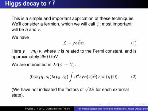
Higgs decay to f f

This is a simple and important application of these techniques.We’ll consider a fermion, which we will call ψ; most importantwill be b and τ .

We haveL = yφψψ. (1)

Here y = mf/v , where v is related to the Fermi constant, and isapproximately 250 GeV.

We are interested inM(φ→ f f ).

〈0|a(p1, s1)b(p2, s2)

∫d4zyφ(z)ψ(z)a†(q)|0〉. (2)

(We have not indicated the factors of√

2E for each externalstate).

Physics 217 2012, Quantum Field Theory Feynman Diagrams for Fermions and Bosons: Higgs Decay and QED

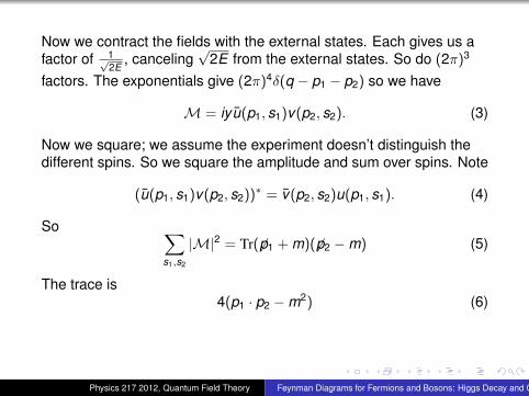
Now we contract the fields with the external states. Each gives us afactor of 1√

2E, canceling

√2E from the external states. So do (2π)3

factors. The exponentials give (2π)4δ(q − p1 − p2) so we have

M = iy u(p1, s1)v(p2, s2). (3)

Now we square; we assume the experiment doesn’t distinguish thedifferent spins. So we square the amplitude and sum over spins. Note

(u(p1, s1)v(p2, s2))∗ = v(p2, s2)u(p1, s1). (4)

So ∑s1,s2

|M|2 = Tr( 6p1 + m)(6p2 −m) (5)

The trace is4(p1 · p2 −m2) (6)

Physics 217 2012, Quantum Field Theory Feynman Diagrams for Fermions and Bosons: Higgs Decay and QED

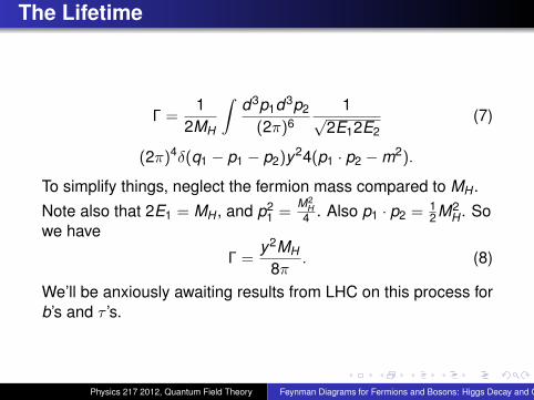
The Lifetime

Γ =1

2MH

∫d3p1d3p2

(2π)61√

2E12E2(7)

(2π)4δ(q1 − p1 − p2)y24(p1 · p2 −m2).

To simplify things, neglect the fermion mass compared to MH .Note also that 2E1 = MH , and p2

1 =M2

H4 . Also p1 · p2 = 1

2M2H . So

we have

Γ =y2MH

8π. (8)

We’ll be anxiously awaiting results from LHC on this process forb’s and τ ’s.

Physics 217 2012, Quantum Field Theory Feynman Diagrams for Fermions and Bosons: Higgs Decay and QED

Quantum Electrodynamics

Now the interaction lagrangian is:

L = −eψγµψAµ. (9)

Using the “contraction" idea, we can write the Feynman rulesfor the S-matrix in quantum electrodynamics.

Physics 217 2012, Quantum Field Theory Feynman Diagrams for Fermions and Bosons: Higgs Decay and QED

Applications: Coulomb Scattering

We consider Coulomb scattering of a particle (initial and finalmomenta p and p′ and positron (initial and final momenta k andk ′) The basic amplitude is

M = i2e2u(p′,a′)γµu(p, s)−igµν

q2 v(k , s)γνv(k ′, s′) (10)

plus an annihilation diagram (we will deal with annihilationshortly; at small impact parameters the term above dominates.Now consider the non-relativistic limit. Up to terms of orderv i = pi

m , the spinors are very simple, and only the γ0 termcontributes, giving

M = −e2

~q2 δs,s′δs,s′ . (11)

The Fourier transform of this amplitude is the Coulombpotential.

Physics 217 2012, Quantum Field Theory Feynman Diagrams for Fermions and Bosons: Higgs Decay and QED

Applications: e+e− → µ+µ−

This is an important process experimentally (with muonsreplaced by quarks it is an important part of our understandingof QCD). The amplitude is

M = −i3v(p′)γµu(p)u(k)γµv(k ′)1s

(12)

where we have suppressed the spins and s = (p + p′)2 is thetotal center of mass energy squared. Note that in the firstfactor, the spinors are those for the electron; in the second forthe muon. Now we average over initial spins (unpolarizedbeams) and sum over final spins (spin-independentmeasurement). Now when we square, we will encounter

(v(p′)γνu(p))∗ = u(p)γνv(p′) (13)

(follows from γν† = γ0γνγ0), and similarly for the second factor.

Physics 217 2012, Quantum Field Theory Feynman Diagrams for Fermions and Bosons: Higgs Decay and QED

This gives:

14

∑spins

M2 = Tr[(6p+me)γµ(6p′−me)γν ]Tr[(6k +mµ)γµ( 6k ′−mµ)γν ]

(14)

Physics 217 2012, Quantum Field Theory Feynman Diagrams for Fermions and Bosons: Higgs Decay and QED

Trace formulas

To evaluate these expressions, we can use:

Tr(1) = 4 Tr(γµγν) = 4gµν (15)

Tr(γµγνγργσ) = 4(gµνgρσ − gµρgνσ + gµσgνρ) (16)

Tr(γµγνγργσγ5) = 4iεµνρσ. (17)

The trace of an odd number of γ matrices vanishes.

Physics 217 2012, Quantum Field Theory Feynman Diagrams for Fermions and Bosons: Higgs Decay and QED

This yields (simplifying things by neglecting the masses):

14|M|2 = 8[k · p′k ′ · p + k · pk ′ · p′]e

4

s2 . (18)

We can easily compute the cross section in the center of massframe. If θ is the angle between ~k and ~p′,

p ·k = E2(1−cos θ) = p′ ·k ′ p′ ·k = E2(1+cos θ) = p′ ·k (19)

And:

dσ =12×16

∫d3kd3k ′

(2π)6(2E)4 (2π)4δ(p+p′−k−k ′)E4(1+cos2 θ)e4

s2

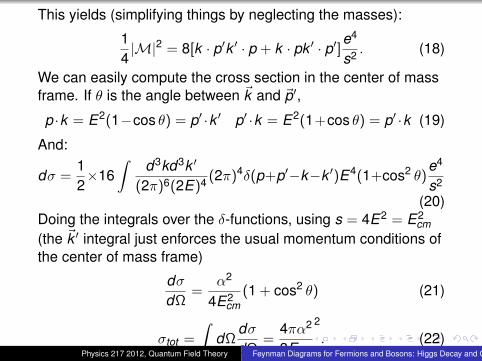
(20)Doing the integrals over the δ-functions, using s = 4E2 = E2

cm(the ~k ′ integral just enforces the usual momentum conditions ofthe center of mass frame)

dσdΩ

=α2

4E2cm

(1 + cos2 θ) (21)

σtot =

∫dΩ

dσdΩ

=4πα2

3Ecm

2

. (22)Physics 217 2012, Quantum Field Theory Feynman Diagrams for Fermions and Bosons: Higgs Decay and QED

e+e− → hadrons; Z 0 → hadrons; leptons

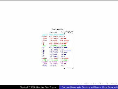
Two applications. Leading computation same as above.Measured rate, Z width.

Physics 217 2012, Quantum Field Theory Feynman Diagrams for Fermions and Bosons: Higgs Decay and QED

Physics 217 2012, Quantum Field Theory Feynman Diagrams for Fermions and Bosons: Higgs Decay and QED

Compton Scattering

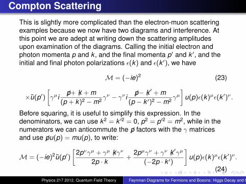
This is slightly more complicated than the electron-muon scatteringexamples because we now have two diagrams and interference. Atthis point we are adept at writing down the scattering amplitudesupon examination of the diagrams. Calling the initial electron andphoton momenta p and k , and the final momenta p′ and k ′, and theinitial and final photon polarizations ε(k) and ε(k ′), we have

M = (−ie)2 (23)

×u(p′)[γµi

6p+ 6k + m(p + k)2 −m2 γ

ν − γν i6p− 6k ′ + m

(p − k ′)2 −m2 γµ

]u(p)ε(k)µε(k ′)ν .

Before squaring, it is useful to simplify this expression. In thedenominators, we can use k2 = k ′2 = 0, p2 = p′2 = m2, while in thenumerators we can anticommute the 6p factors with the γ matricesand use 6pu(p) = mu(p), to write:

M = (−ie)2u(p′)[

2pνγµ + γµ 6kγν

2p · k+

2pµγν + γν 6k ′γµ

(−2p · k ′)

]u(p)ε(k)µε(k ′)ν .

(24)Physics 217 2012, Quantum Field Theory Feynman Diagrams for Fermions and Bosons: Higgs Decay and QED

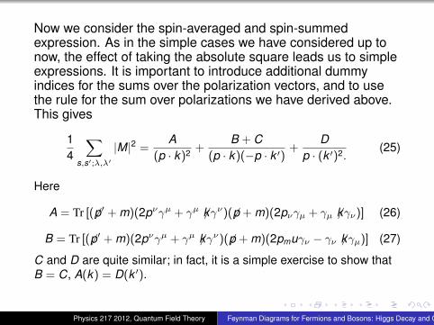
Now we consider the spin-averaged and spin-summedexpression. As in the simple cases we have considered up tonow, the effect of taking the absolute square leads us to simpleexpressions. It is important to introduce additional dummyindices for the sums over the polarization vectors, and to usethe rule for the sum over polarizations we have derived above.This gives

14

∑s,s′;λ,λ′

|M|2 =A

(p · k)2 +B + C

(p · k)(−p · k ′)+

Dp · (k ′)2.

(25)

Here

A = Tr [(6p′ + m)(2pνγµ + γµ 6kγν)( 6p + m)(2pνγµ + γµ 6kγν)] (26)

B = Tr [( 6p′ + m)(2pνγµ + γµ 6kγν)(6p + m)(2pmuγν − γν 6kγµ)] (27)

C and D are quite similar; in fact, it is a simple exercise to show thatB = C, A(k) = D(k ′).

Physics 217 2012, Quantum Field Theory Feynman Diagrams for Fermions and Bosons: Higgs Decay and QED

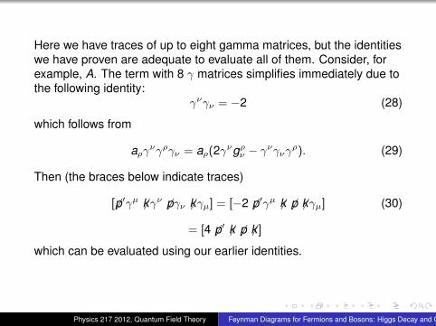
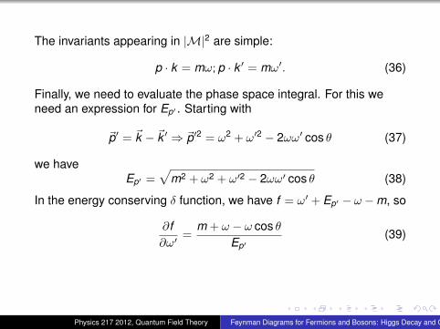
Here we have traces of up to eight gamma matrices, but the identitieswe have proven are adequate to evaluate all of them. Consider, forexample, A. The term with 8 γ matrices simplifies immediately due tothe following identity:

γνγν = −2 (28)

which follows from

aργνγργν = aρ(2γνgρν − γνγνγρ). (29)

Then (the braces below indicate traces)

[6p′γµ 6kγν 6pγν 6kγµ] = [−2 6p′γµ 6k 6p 6kγµ] (30)

= [4 6p′ 6k 6p 6k ]

which can be evaluated using our earlier identities.

Physics 217 2012, Quantum Field Theory Feynman Diagrams for Fermions and Bosons: Higgs Decay and QED

One finds

A = 16(4m4 − 2m2p · p′ + 4m2p · k − 2m2p′ · k + 2p · kp′ · k). (31)

and working through all four terms:

14

∑|M|2 (32)

= 2e4

[p · k ′

p · k+

p · kp · k ′

+ 2m2(

1p · k

− 1p · k ′

)+ m4

(1

p · k− 1

p · k ′

)2].

Now we can work out the cross section in various frames.

Physics 217 2012, Quantum Field Theory Feynman Diagrams for Fermions and Bosons: Higgs Decay and QED

Compton Scattering in the Lab Frame

It is helpful to be methodical and to write the four vectors in detail

k = (ω, ωz) p = (m, ~0) k ′ = (ω′, ω′ sin θ,0, ω′ cos θ).

(Note that this defines the z axis).Then four momentum conservation allows us to solve for ω′:

p′2 = m2 = (p + k − k ′)2 = p2 + 2p · (k − k ′)− 2k · k ′. (33)

Evaluating the invariants in terms of the lab frame ω, ω′, and θ, this is:

0 = 2m(ω − ω′)− 2ωω′(1− cos θ). (34)

Solving for ω′:ω′ =

ω

1 + ωm (1− cos θ)

. (35)

Physics 217 2012, Quantum Field Theory Feynman Diagrams for Fermions and Bosons: Higgs Decay and QED

The invariants appearing in |M|2 are simple:

p · k = mω; p · k ′ = mω′. (36)

Finally, we need to evaluate the phase space integral. For this weneed an expression for Ep′ . Starting with

~p′ = ~k − ~k ′ ⇒ ~p′2 = ω2 + ω′2 − 2ωω′ cos θ (37)

we haveEp′ =

√m2 + ω2 + ω′2 − 2ωω′ cos θ (38)

In the energy conserving δ function, we have f = ω′ + Ep′ − ω −m, so

∂f∂ω′

=m + ω − ω cos θ

Ep′(39)

Physics 217 2012, Quantum Field Theory Feynman Diagrams for Fermions and Bosons: Higgs Decay and QED

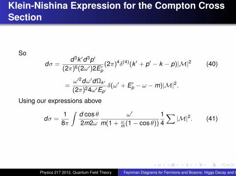
Klein-Nishina Expression for the Compton CrossSection

So

dσ =d3k ′d3p′

(2π)6(2ω′)2E ′p(2π)4δ(4)(k ′ + p′ − k − p)|M|2 (40)

=ω′2dω′dΩk ′

(2π)24ω′Ep′δ(ω′ + E ′p − ω −m)|M|2.

Using our expressions above

dσ =1

8π

∫d cos θ2m2ω

ω′

m(1 + ωm (1− cos θ))

14

∑|M|2. (41)

Physics 217 2012, Quantum Field Theory Feynman Diagrams for Fermions and Bosons: Higgs Decay and QED

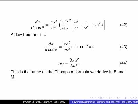
dσd cos θ

=πα2

m2

(ω′

ω

)2 [ω′ω

+ω

ω′− sin2 θ

]. (42)

At low frequencies:

dσd cos θ

=πα2

m2 (1 + cos2 θ). (43)

σtot =8πα2

3m2 . (44)

This is the same as the Thompson formula we derive in E andM.

Physics 217 2012, Quantum Field Theory Feynman Diagrams for Fermions and Bosons: Higgs Decay and QED

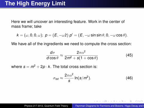
The High Energy Limit

Here we will uncover an interesting feature. Work in the center ofmass frame; take

k = (ω,0,0, ω); p = (E ,−ωz) p′ = (E ,−ω sin sin θ,0,−ω cos θ).

We have all of the ingredients we need to compute the cross section:

dσd cos θ

≈ 2πα2

2m2 + s(1 + cos θ)(45)

where s = m2 + 2p · k . The total cross section is:

σtot ≈2πα2

sln(s/m2). (46)

Physics 217 2012, Quantum Field Theory Feynman Diagrams for Fermions and Bosons: Higgs Decay and QED

Colinear Singularities

Why the singularity as m→ 0. Should be able to see a problemif set m = 0 from the start problem comes when 2p · k or2p · k ′ = 0. Corresponds to p along k or k ′. The precise form ofthe singularity requires understanding the behavior of thespinors u(p) (see Peskin and Schroder).

Physics 217 2012, Quantum Field Theory Feynman Diagrams for Fermions and Bosons: Higgs Decay and QED