60
Data Analysis in Systematic Reviews Madhukar Pai, MD, PhD Associate Professor McGill University Montreal Email: [email protected]

Data Analysis in Systematic
Reviews
Madhukar Pai, MD, PhD
Associate Professor
McGill University
Montreal
Email: [email protected]

Central questions of interest
Are the results of the
studies fairly similar
(consistent)?
Yes No
What is the common,
summary effect?
How precise is the
common, summary
effect?
What factors can
explain the
dissimilarities
(heterogeneity) in the
study results?

Steps in data analysis & presentation
1. Tabulate summary data
2. Graph data
3. Check for heterogeneity
4. Perform a meta-analysis if heterogeneity is not a major concern
5. If heterogeneity is found, identify factors that can explain it
6. Evaluate the impact of study quality on results
7. Explore the potential for publication bias
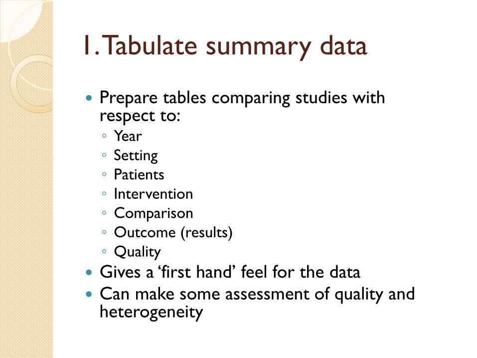
1. Tabulate summary data
Prepare tables comparing studies with respect to: ◦ Year
◦ Setting
◦ Patients
◦ Intervention
◦ Comparison
◦ Outcome (results)
◦ Quality
Gives a ‘first hand’ feel for the data
Can make some assessment of quality and heterogeneity

Tabulate summary data
Example: Cochrane albumin review
Study Year Patient
populati
on
Intervent
ion
Compari
son
Summary
measure
(RR)
Allocation
concealm
ent
Lucas et
al.
1978 Trauma Albumin No
albumin
13.9 Inadequat
e
Jelenko
et al.
1979 Burns Albumin Ringer’s
lactate
0.50 Unclear
Rubin et
al.
1997 Hypoalbu
minemia
Albumin No
albumin
1.9 Adequate
Cochrane Injuries Group Albumin Reviewers. Human albumin administration in critically ill
patients: systematic review of randomised controlled trials. BMJ 1998;317:235-40.

2. Graph summary data
Efficient way of presenting summary results
Forest plot: ◦ Presents the point estimate and CI of each trial
◦ Also presents the overall, summary estimate
◦ Allows visual appraisal of heterogeneity
Other graphs: ◦ Cumulative meta-analysis
◦ Sensitivity analysis
◦ Funnel plot for publication bias
◦ Galbraith, L’Abbe plots, etc [rarely used]

Forest Plot
Bates et al. Arch Intern Med 2007

Ried K. Aus Fam Phys 2006

Ried K. Aus Fam Phys 2006

Ried K. Aus Fam Phys 2006
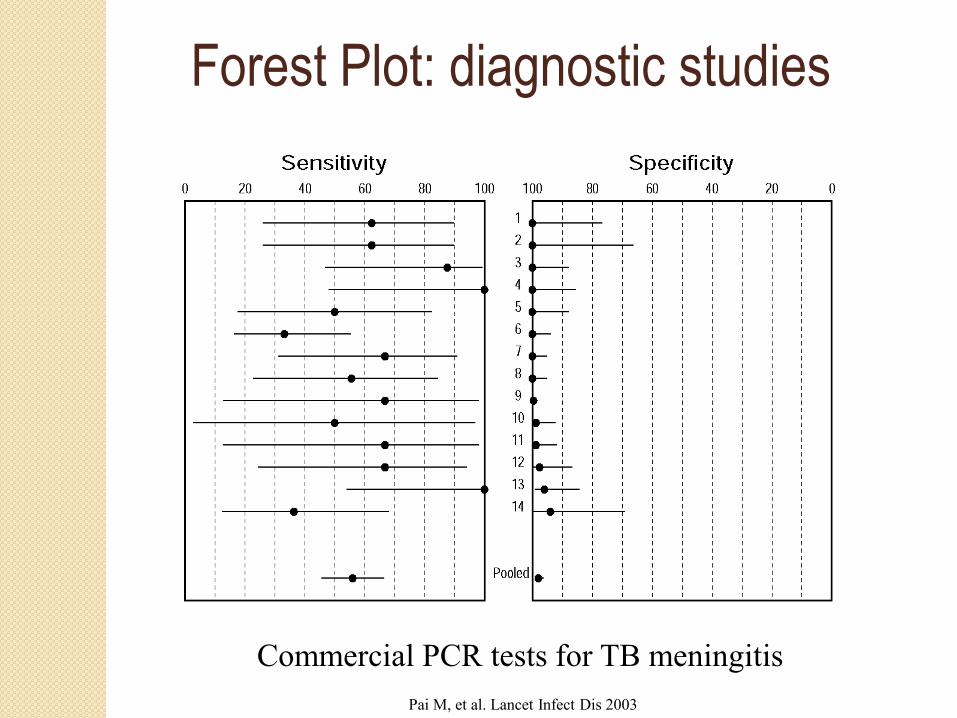
Commercial PCR tests for TB meningitis
Pai M, et al. Lancet Infect Dis 2003
Forest Plot: diagnostic studies
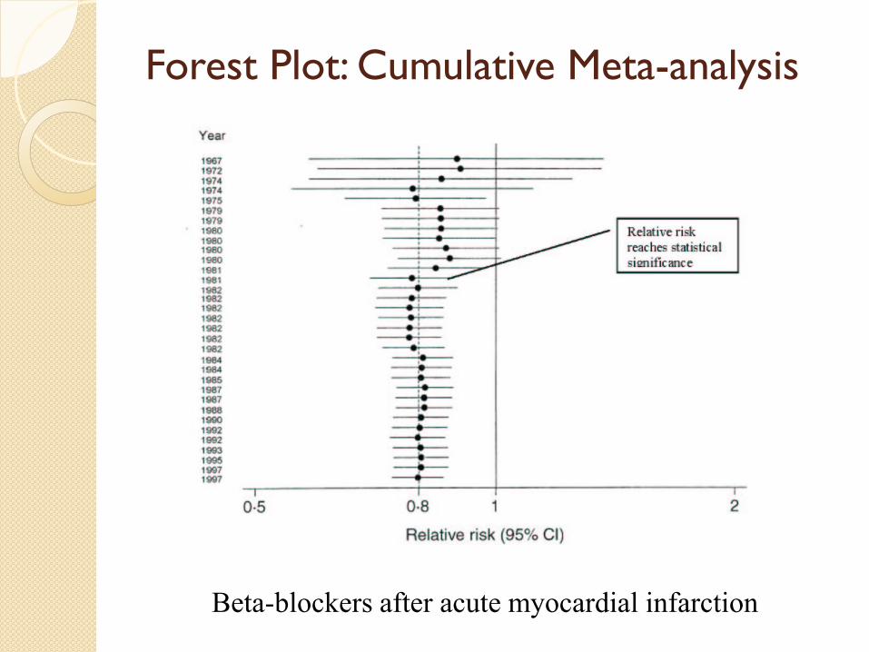
Forest Plot: Cumulative Meta-analysis
Beta-blockers after acute myocardial infarction

0.01 0.1 1 10 100
Odds Ratios with 95% Confidence Intervals
Favours Aprotinin Favours Control
Ref #
Year of
Publication # Pts
6 7 8 9
10 11 12 13 14 15 16 17 18 19 20 21 22 23 24 25 26a 26b 27 28 29 30 31 32 33 34 35 36 37 38 39 40 41 42 43 44 45 46 47 48 49 50 51 52 53 54 55 56 57a 57b 58 59 60 61 62 63 64 65 66
22 99
175 219 257 296 376 396 455 486 601
2385 2445 2495 2664 2754 2795 3005 3044 3146 3201 3342 3396 3475 3575 3668 3724 3822 3854 3882 4047 4147 4210 4240 4338 4382 4420 4450 4548 4578 4832 4882 4975 5023 5135 5326 5970 6008 6060 6227 6333 6376 6442 6507 7303 7360 7510 7593 7677 7697 7897 7952 8011 8040
Cumulative Meta-Analysis of all RCTs
Dec - 87 Mar - 89 Apr - 89
Sep - 90 Oct - 90 Dec - 90 Jun - 91 Sep - 91 Dec - 91 Apr - 92 Jun - 92 Jun - 92 Jun - 92 Nov - 92 Dec - 92 Jan - 93 Jul - 93
Aug - 93 Dec - 93 Jan - 94 Feb - 94 Feb - 94 Feb - 94 Apr - 94 Jul - 94
Aug - 94 Aug - 94 Oct - 94 Oct - 94
Dec - 94 Dec - 94 Feb - 95 Feb - 95 Feb - 95 Apr - 95 Jun - 95 Jun - 95 Sep - 95 Oct - 95 Oct - 95 Oct - 95
May - 96 Jul - 96
Aug - 96 Aug - 96 Oct - 96
Dec - 96 Jan - 97 Jan - 97 Aug - 97 Sep - 97 Dec - 97 Oct - 98 Oct - 98
Nov - 98 Aug - 99 Sep - 99 Mar - 00 Dec - 00 Dec - 00 Jan - 01 Sep - 01 Sep - 01 Jun - 02 0.34 (0.29, 0.41)
0.33 (0.26, 0.41)
0.30 (0.24, 0.38)
0.29 (0.23, 0.38)
0.28 (0.20, 0.38)
0.22 (0.09, 0.52)
0.11 (0.03, 0.38)
67
Fergusson D et al. Clinical Trials 2005; 2: 218–232
Aprotinin
for cardiac
surgery
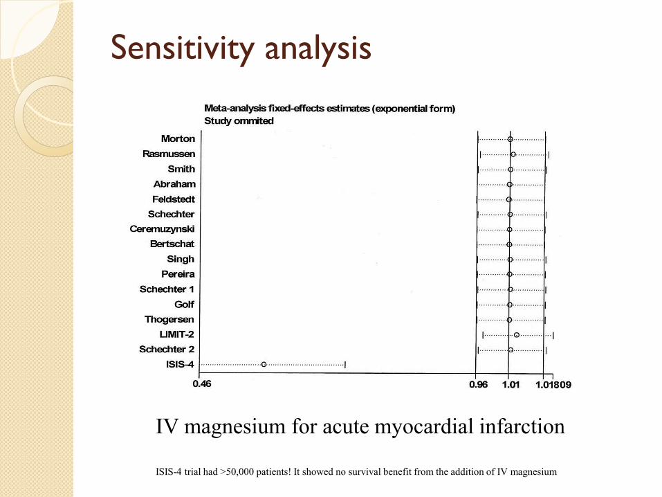
Sensitivity analysis
IV magnesium for acute myocardial infarction
ISIS-4 trial had >50,000 patients! It showed no survival benefit from the addition of IV magnesium

3. Check for heterogeneity
Indicates that effect varies a lot across studies
If heterogeneity is present, a common, summary measure is hard to interpret
Statistical vs clinical heterogeneity Can be due to due to differences in: ◦ Patient populations studied ◦ Interventions used ◦ Co-interventions ◦ Outcomes measured ◦ Study design features (eg. length of follow-up) ◦ Study quality ◦ Random error
“Average men having an average meal”
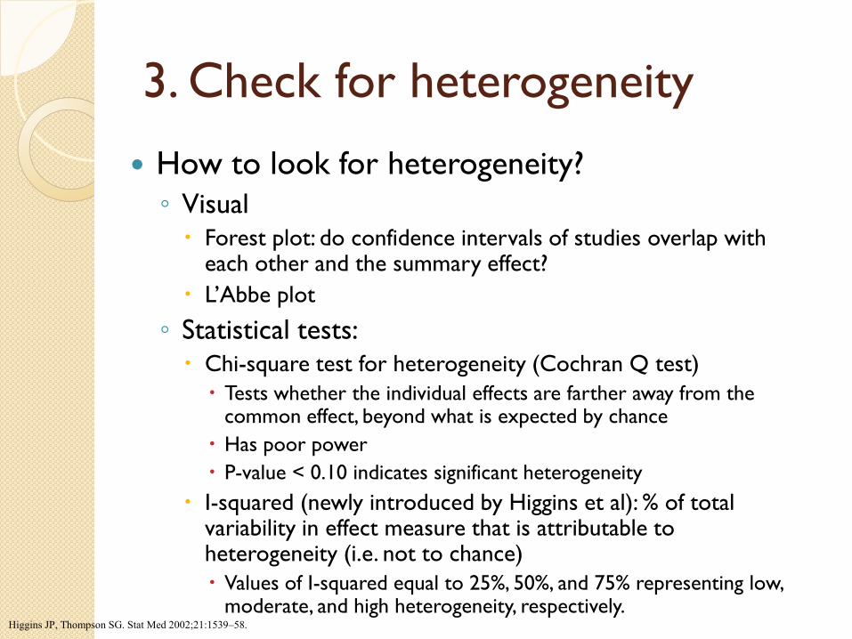
3. Check for heterogeneity
How to look for heterogeneity?
◦ Visual Forest plot: do confidence intervals of studies overlap with
each other and the summary effect?
L’Abbe plot
◦ Statistical tests: Chi-square test for heterogeneity (Cochran Q test)
Tests whether the individual effects are farther away from the common effect, beyond what is expected by chance
Has poor power
P-value < 0.10 indicates significant heterogeneity
I-squared (newly introduced by Higgins et al): % of total variability in effect measure that is attributable to heterogeneity (i.e. not to chance)
Values of I-squared equal to 25%, 50%, and 75% representing low, moderate, and high heterogeneity, respectively.
Higgins JP, Thompson SG. Stat Med 2002;21:1539–58.

Visual appraisal of heterogeneity
Bates et al. Arch Intern Med 2007
Association between smoking and TB mortality
P-value for heterogeneity <0.001

Chartrand C et al. Annals 2012

L’Abbe plot for heterogeneity Trials in which the
experimental treatment
proves better than the
control (EER > CER) will
be in the upper left of the
plot, between the y axis
and the line of equality
(Figure). If experimental is
no better than control
then the point will fall on
the line of equality (EER =
CER), and if control is
better than experimental
then the point will be in
the lower right of the
plot, between the x axis
and the line of equality
(EER < CER).
http://www.medicine.ox.ac.uk/bandolier/booth/glossary/labbe.html

3. Check for heterogeneity
If significant heterogeneity is found:
◦ Find out what factors might explain the
heterogeneity
◦ Can decide not to combine the data
If no heterogeneity:
◦ Can perform meta-analysis and generate a
common, summary effect measure

Heterogeneity makes it hard to interpret
pooled estimates
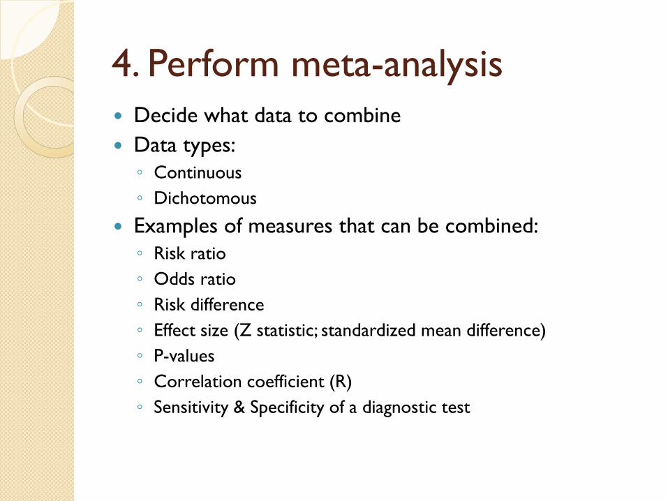
4. Perform meta-analysis
Decide what data to combine
Data types:
◦ Continuous
◦ Dichotomous
Examples of measures that can be combined:
◦ Risk ratio
◦ Odds ratio
◦ Risk difference
◦ Effect size (Z statistic; standardized mean difference)
◦ P-values
◦ Correlation coefficient (R)
◦ Sensitivity & Specificity of a diagnostic test

4. Perform meta-analysis
Statistical models for combining data:
◦ All methods are essentially compute weighted
averages
◦ Weighting factor is often the study size
◦ Models:
Fixed effects model
Inverse-variance, Peto method, M-H method
Random effects model
DerSimonian & Laird method


Courtesy: Leon Bax, http://www.mix-for-meta-analysis.info/index.html#

4. Perform meta-analysis
Fixed effects model
◦ based on the assumption that a single common (or 'fixed') effect underlies every study in the meta-analysis
◦ For example, if we were doing a meta-analysis of ORs, we would assume that every study is estimating the same OR.
◦ Under this assumption, if every study were infinitely large, every study would yield an identical result.
◦ Same as assuming there is no statistical heterogeneity among the studies


Example of a fixed effects method (M-H)
Disease
Treat
ment
+
-
+
a
b
-
c
d
Disease
Treat
ment
+
-
+
a
b
-
c
d
Study 1 Study 2

Example of a fixed effects method (M-H)
Disease
Treat
ment
+
-
+
10
90
-
20
80
Disease
Treat
ment
+
-
+
12
88
-
16
84
Study 1: n1 = 200 Study 2: n2 = 200
OR = 0.44 OR = 0.72
= (4+5.04) / (9+7.04) = ORMH = 0.56

4. Perform meta-analysis
Random effects model ◦ Makes the assumption that individual studies are estimating
different true effects
we assume they have a distribution with some central value and some
degree of variability
the idea of a random effects MA is to learn about this distribution of
effects across different studies
Random effects model: Allows for random error plus inter-study variability
Results in wider confidence intervals (conservative)
Studies tend to be weighted more equally (relatively more weight is
given to smaller studies)
Can be unpredictable (i.e. not stable)


R. DerSimonian and N. Laird, Meta-analysis in clinical trials, Controlled Clinical Trials 7 (1986), pp. 177–188
DerSimonian and Laird Model

4. Perform meta-analysis
Moher D et al. Arch Pediatr Adolesc Med 1998;152:915-20

5. Identify factors that can explain
heterogeneity
If heterogeneity is found, use these approaches to identify factors that can explain it:
◦ Graphical methods
◦ Subgroup analysis
◦ Sensitivity analysis
◦ Meta-regression
Of all these approaches, subgroup analysis is easily done and interpreted

Graphical exploration
Meta-analysis on efficacy of BCG vaccination for TB
I-squared = 92%

This photo is of a sign located on Interstate 89 in
Vermont just south of the border with Quebec
Province, Canada [source: Wikipedia]

Subgroup analysis: example
Egger et al. Systematic reviews in health care. London: BMJ books, 2001.

Subgroup analysis: example
Egger et al. Systematic reviews in health care. London: BMJ books, 2001.
Beta-carotene intake and cardiovascular mortality

Subgroup analysis: example
“Considerable heterogeneity was found in the pooled estimates, as expected. Despite our attempts
to explain it through the regression model, substantial heterogeneity remained unexplained.”

Exploring heterogeneity using meta-
regression
A meta-regression can be either a linear or logistic
regression model
◦ Can be weighted or unweighted
Unit of analysis is a study (similar to an ecological
study).
Outcome variable: effect (e.g. log odds ratio)
Covariates: study-level variables (e.g. Study quality, mean
age of participants, etc)
Model: log OR = a + b1X1 + b2X2 + b3X3
where, X1, X2, etc are study level covariates
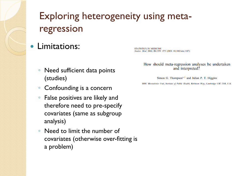
Exploring heterogeneity using meta-
regression
Limitations:
◦ Need sufficient data points
(studies)
◦ Confounding is a concern
◦ False positives are likely and
therefore need to pre-specify
covariates (same as subgroup
analysis)
◦ Need to limit the number of
covariates (otherwise over-fitting is
a problem)

6. Evaluate impact of study quality on
results
Narrative discussion of impact of quality on results
Display study quality and results in a tabular format
Weight the data by quality (not recommended)
Subgroup analysis by quality
Include quality as a covariate in meta-regression

New Yorker, 1966

7. Explore publication bias
Studies with significant results are more likely ◦ to be published
◦ to be published in English
◦ to be cited by others
◦ to produce multiple publications
Including only published studies can introduce publication bias
Most reviews do not look for publication bias
Methods for detecting publication bias: ◦ Graphical: funnel plot asymmetry
◦ Tests: Egger test, Rosenthal’s Fail-safe N [all have low power]

Montori et al. Mayo Clin Proc 2000

Montori et al. Mayo Clin Proc 2000
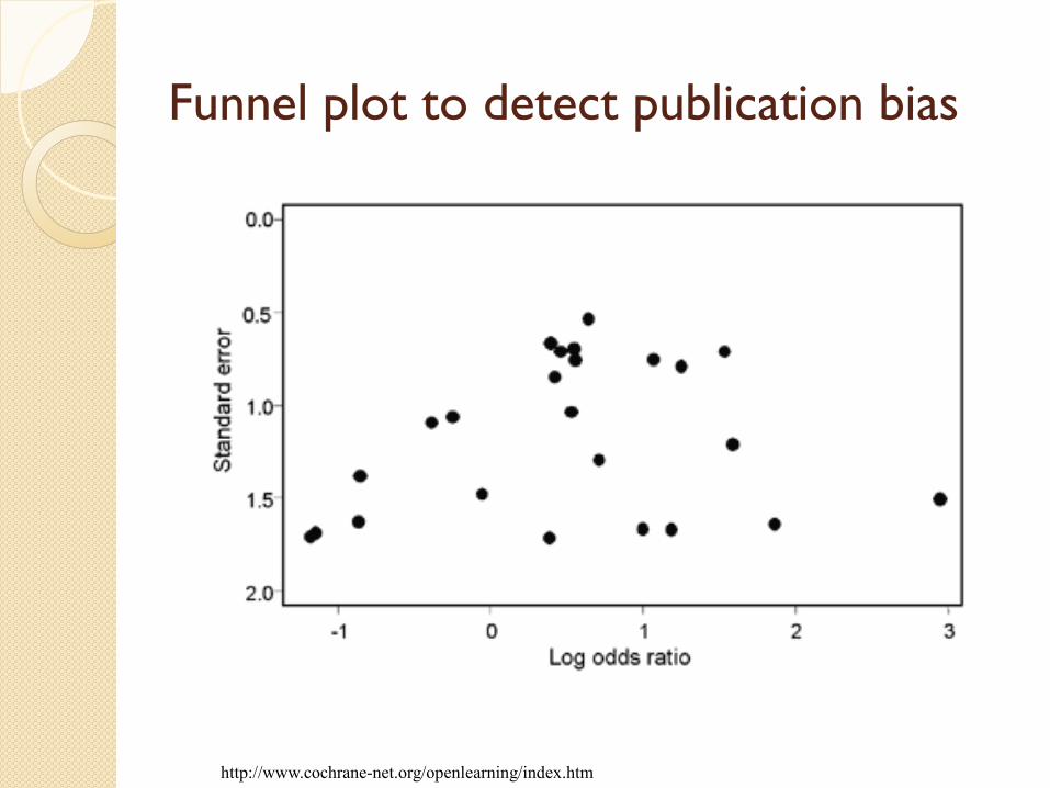
Funnel plot to detect publication bias
http://www.cochrane-net.org/openlearning/index.htm

Funnel plot to detect publication bias
http://www.cochrane-net.org/openlearning/index.htm

Testing for funnel plot asymmetry
Ntot is the total sample size, NE and NC are the sizes of the experimental and control intervention groups, S is the total
number of events across both groups and F = Ntot – S. Note that only the first three of these tests (Begg 1994, Egger 1997a,
Tang 2000) can be used for continuous outcomes.
http://handbook.cochrane.org/
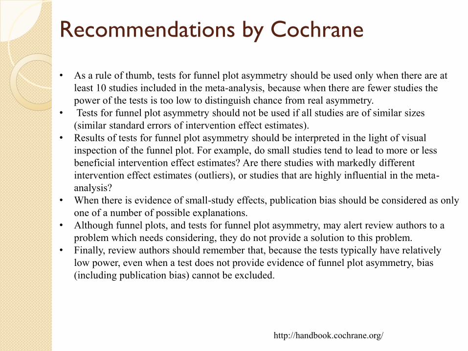
Recommendations by Cochrane
http://handbook.cochrane.org/
• As a rule of thumb, tests for funnel plot asymmetry should be used only when there are at
least 10 studies included in the meta-analysis, because when there are fewer studies the
power of the tests is too low to distinguish chance from real asymmetry.
• Tests for funnel plot asymmetry should not be used if all studies are of similar sizes
(similar standard errors of intervention effect estimates).
• Results of tests for funnel plot asymmetry should be interpreted in the light of visual
inspection of the funnel plot. For example, do small studies tend to lead to more or less
beneficial intervention effect estimates? Are there studies with markedly different
intervention effect estimates (outliers), or studies that are highly influential in the meta-
analysis?
• When there is evidence of small-study effects, publication bias should be considered as only
one of a number of possible explanations.
• Although funnel plots, and tests for funnel plot asymmetry, may alert review authors to a
problem which needs considering, they do not provide a solution to this problem.
• Finally, review authors should remember that, because the tests typically have relatively
low power, even when a test does not provide evidence of funnel plot asymmetry, bias
(including publication bias) cannot be excluded.

Meta-analysis Software
Free
◦ RevMan 5 [Review Manager]
◦ Meta-Analyst
◦ Epi Meta
◦ Easy MA
◦ Meta-DiSc
◦ Meta-Stat
Commercial
◦ Comprehensive Meta-analysis Version 2
◦ MIX 2.0 Pro
◦ Meta-Win
◦ WEasy MA
General stats packages (commercial)
◦ Stata
◦ SAS
◦ R
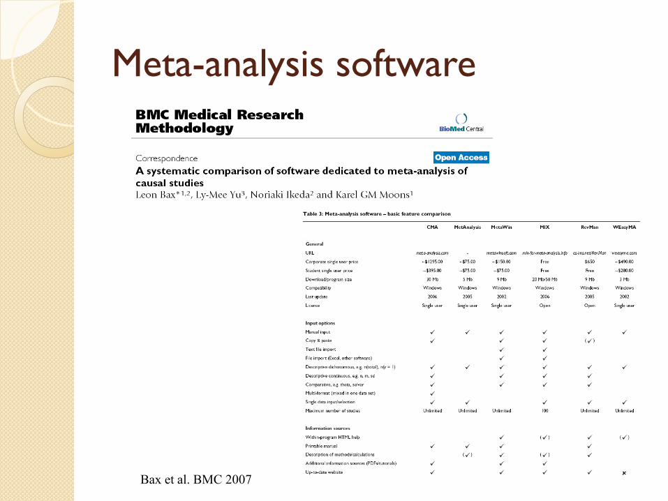
Meta-analysis software
Bax et al. BMC 2007

RevMan 5

http://www.meta-analysis-made-easy.com/
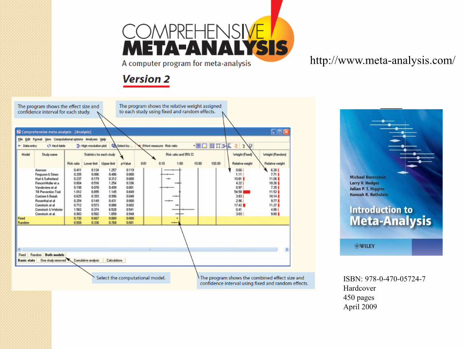
http://www.meta-analysis.com/
ISBN: 978-0-470-05724-7
Hardcover
450 pages
April 2009

60


