DATA-DRIVEN MODEL PREDICTIVE CONTROL OF LOW-LIFT CHILLERS PRE-COOLING THERMO-ACTIVE BUILDING SYSTEMS Nick Gayeski, PhD Building Technology, MIT IBPSA Model Predictive Control Workshop June 2011 Advisors: Dr. Leslie K. Norford, Dr. Peter R. Armstrong
Transcript
DATA-DRIVEN MODEL PREDICTIVE CONTROL OF LOW-LIFT CHILLERS PRE-COOLING THERMO-ACTIVE BUILDING SYSTEMS
Nick Gayeski, PhD Building Technology, MIT
IBPSA Model Predictive Control Workshop June 2011
Advisors: Dr. Leslie K. Norford, Dr. Peter R. Armstrong
Objective and Topics
Objective: To achieve significant cooling energy savings with data-driven model-predictive control of low-lift chillers pre-cooling thermo-active building systems (TABS)
1. Low-lift cooling systems (LLCS)
2. Modeling and optimization for LLCSa. Low-lift chiller performance
b. Data-driven thermal model identification
c. Model-predictive control to pre-cool thermo-active building systems
Low lift cooling systems leverage the following technologies to reduce cooling energy:
Variable speed compressor Hydronic distribution with variable flow Radiant cooling Thermal energy storage (TES) e.g. Thermo-active
building systems (TABS) Model-predictive control (MPC) to pre-cool TABS Dedicated outdoor air system (DOAS)
Nick Gayeski IBPSA MPC Workshop June, 2011
0
20
40
T
-
Tem
pera
ture
(°C
)
60
1 1.2 1.4S - Entropy (kJ/kg-K)
1.6 1.8
100
200
300
400500600700 psia
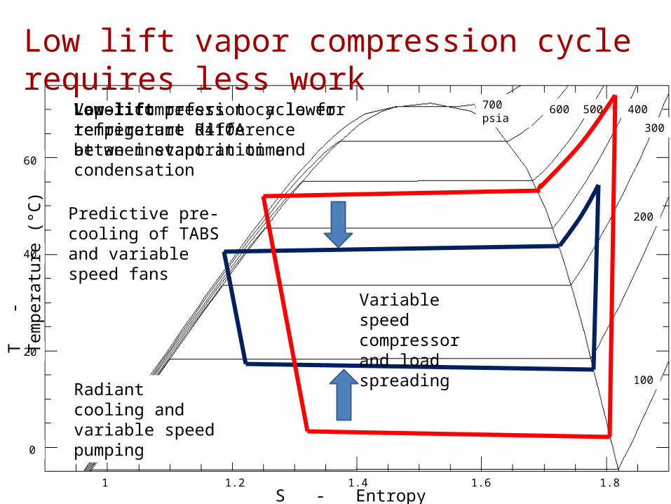
Radiant cooling and variable speed pumping
Predictive pre-cooling of TABS and variable speed fans
Low-lift refers to a lower temperature difference between evaporation and condensation
Variable speed compressor and load spreading
Low lift vapor compression cycle requires less work
Vapor compression cycle for refrigerant R410A at an instant in time
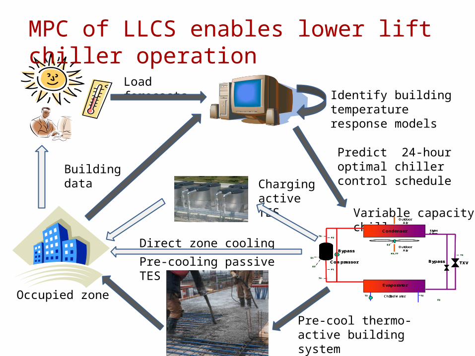
Predict 24-hour optimal chiller control schedule
Variable capacity chiller
Load forecasts
Building data
Identify building temperature response models
Charging active TES
Direct zone coolingCompressor
Condenser
Evaporator
TXV
Sight Glass
Outdoor Air
Outdoor Air
E1
E2
E3
T5
T6
T4
P1
P2
H3, T7
Chilled Water T2T3
F3
Bypass
BypassCompressor
Condenser
Evaporator
TXV
Sight Glass
Outdoor Air
Outdoor Air
E1
E2
E3
T5
T6
T4
P1
P2
H3, T7
Chilled Water T2T3
F3
Bypass
Bypass
Pre-cool thermo-active building system
Pre-cooling passive TES
MPC of LLCS enables lower lift chiller operation
Occupied zone
Simulation studies show significant LLCS cooling energy savings potentialSimulated energy savings: 12 building types in 16 cities relative to a DOE benchmark HVAC system
Total annual cooling energy savings 37 to 84% in standard buildings, on average 60-
70% -9 to 70% in high performance buildings, on
average 40-60%
Katipamula S, Armstrong PR, Wang W, Fernandez N, Cho H, Goetzler W,Burgos J, Radhakrishnan R, Ahlfeldt C. 2010. Cost-Effective Integration of Efficient Low-Lift Baseload Cooling Equipment FY08 Final Report. PNNL-19114. Pacific Northwest National Laboratory. Richland, WA.
Nick Gayeski IBPSA MPC Workshop June, 2011
Topics
Model-predictive control of low-lift cooling systems to achieve significant cooling energy savings1. Low-lift cooling systems (LLCS)
2. Modeling and optimization for LLCSa. Low-lift chiller performance
b. Data-driven thermal model identification
c. Model-predictive control to pre-cool thermo-active building systems
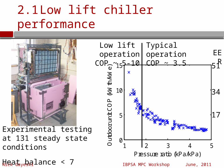
Empirical models accurately represent chiller cooling capacity and power
20 30 40 50 60 70 80 900
0.1
0.2
0.3
0.4
0.55/35
Compressor Speed (Hz)
1/C
OP
(W
e/Wth
)
1/COP vs Compressor Speed at Fan Speed = 750 RPM Te/T
o
20 30 40 50 60 70 80 900
0.1
0.2
0.3
0.4
0.5
5/25
5/35
Compressor Speed (Hz)
1/C
OP
(W
e/Wth
)
1/COP vs Compressor Speed at Fan Speed = 750 RPM Te/T
o
20 30 40 50 60 70 80 900
0.1
0.2
0.3
0.4
0.5
5/25
5/35
10/25
Compressor Speed (Hz)
1/C
OP
(W
e/Wth
)
1/COP vs Compressor Speed at Fan Speed = 750 RPM Te/T
o
Night time operation
Radiant cooling
Te = Evaporating temperature ºC, To = Outdoor air temperature ºC
Load spreading
MPC with TABS enables more low-lift operation, resulting in higher chiller COPs
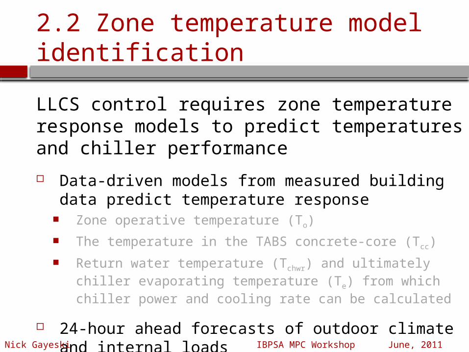
2.2 Zone temperature model identification
LLCS control requires zone temperature response models to predict temperatures and chiller performance
Data-driven models from measured building data predict temperature response
Zone operative temperature (To)
The temperature in the TABS concrete-core (Tcc)
Return water temperature (Tchwr) and ultimately chiller evaporating temperature (Te) from which chiller power and cooling rate can be calculated
24-hour ahead forecasts of outdoor climate and internal loads
Nick Gayeski IBPSA MPC Workshop June, 2011
To = operative temperatureTx = outdoor air temperatureTa = adjacent zone air temperatureQi = heat rate from internal loadsQc = cooling rate from mechanical
systema,b,c,d,e = weights for time series of
each variable
(Inverse) comprehensive room transfer function (CRTF) [Seem 1987]
Steady state heat transfer physics constrain CRTF coefficients
Nt
tk
ck
Nt
tk
ik
Nt
tk
ak
Nt
1tk
Nt
tk
xkoko )k(Qe)k(Qd)k(Tc)k(Tb)k(Ta)t(T
Existing data-driven modeling methods can be applied to predict zone temperature
Nick Gayeski IBPSA MPC Workshop June, 2011
Chiller power and cooling rate depend on TABS thermal state and cooling rate because they determines chilled water return temperature and evaporating temperature
Predict concrete-core temperature (Tcc) using a CRTF like transfer function model
Predict return water temperature (Tchwr) using a low-order transfer function model in Tcc and cooling rate Qc (or a heat exchanger model)
Superheat relates Tchwr to evaporating temperature (Te)
Evaporating temperature must be predicted from TABS temperature response
Nick Gayeski IBPSA MPC Workshop June, 2011
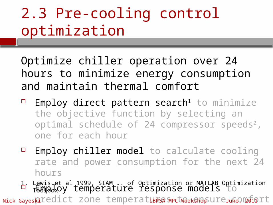
2.3 Pre-cooling control optimization
Optimize chiller operation over 24 hours to minimize energy consumption and maintain thermal comfort Employ direct pattern search1 to minimize the
objective function by selecting an optimal schedule of 24 compressor speeds2, one for each hour
Employ chiller model to calculate cooling rate and power consumption for the next 24 hours
Employ temperature response models to predict zone temperatures to ensure comfort is maintained over 24 hours
1. Lewis et al 1999, SIAM J. of Optimization or MATLAB Optimization Toolbox
Nick Gayeski IBPSA MPC Workshop June, 2011
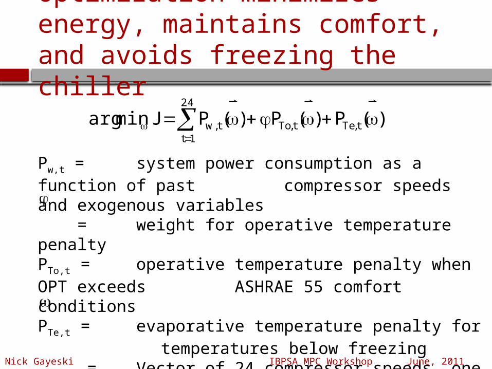
Pw,t = system power consumption as a function of past compressor speeds and exogenous variables = weight for operative temperature penaltyPTo,t = operative temperature penalty when OPT exceeds ASHRAE 55 comfort conditionsPTe,t = evaporative temperature penalty for
temperatures below freezing = Vector of 24 compressor speeds, one for each hour of the 24 hours ahead
24
1tt,Tet,Tot,w )(P)(P)(PJminarg
Optimization minimizes energy, maintains comfort, and avoids freezing the chiller
Nick Gayeski IBPSA MPC Workshop June, 2011
Pattern search initial guess at current hour
Pattern search algorithm determines optimal
compressor speed schedule for the next 24 hours
Operate chiller for one hour at optimal state
24-hour-ahead forecasts of outdoor air temperature, adjacent zone temperatures, and internal loads optimal241ioptimal
optimal,1
)T,T,(ff chwrxoptimal,1
0,optimal242iinitial
Optimize compressor speeds every hour with updated building data and forecasts
Nick Gayeski IBPSA MPC Workshop,June, 2011
Topics
Model-predictive control of low-lift cooling systems to achieve significant cooling energy savings1. Low-lift cooling systems (LLCS)
2. Implementing MPC for LLCSa. Low-lift chiller performance
b. Data-driven thermal model identification
c. Model-predictive control to pre-cool thermo-active building systems
Foundational research shows dramatic savings from LLCS, but
Assumes idealized thermal storage, not real TES or TABS
Chiller power and cooling rate are not coupled to thermal storage, as it can be for a TABS system
How real are these savings? What practical technical obstacles exist?
Experimentally implement and test LLCS with MPC pre-cooling TABS
Check relative savings of LLCS to a base case system similar to comparisons in the PNNL simulation research
Nick Gayeski IBPSA MPC Workshop June, 2011
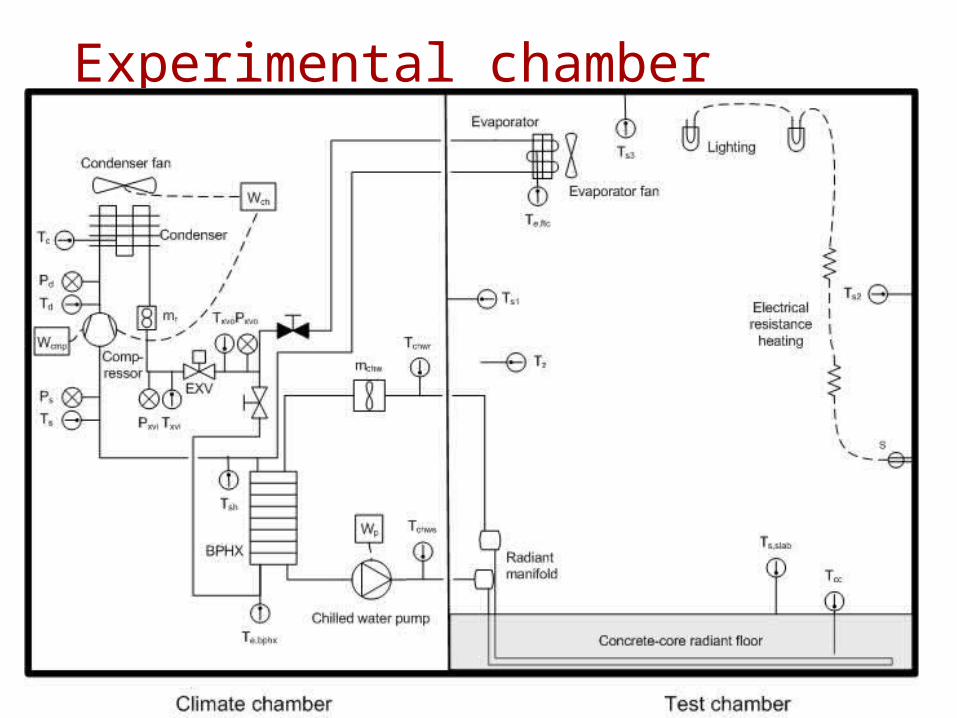
IDENTICAL FOR LLCS AND BASE CASE SSAC
Experimental chamber schematic
Climate chamber
Test chamber
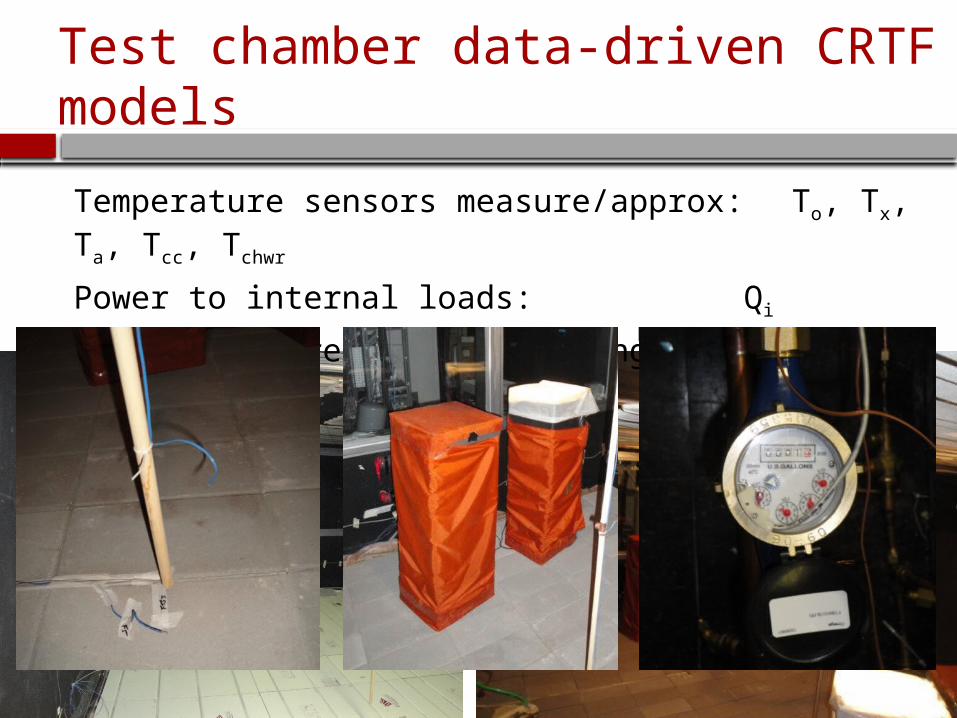
Temperature sensors measure/approx: To, Tx, Ta, Tcc, Tchwr
Power to internal loads: Qi
Radiant concrete floor cooling rate: Qc
Test chamber data-driven CRTF models
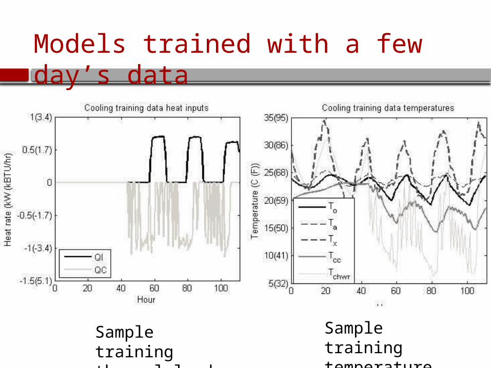
Sample training temperature data
Sample training thermal load data
Models trained with a few day’s data
Transfer function models accurately predict zone temperatures 24-hours-ahead
Nick Gayeski IBPSA MPC Workshop June, 2011
24-hour TABS and chilled water temperature prediction
24 hour operative temperature prediction
Atlanta typical summer week with standard efficiency loads
Phoenix typical summery week with high efficiency loads Based on typical meteorological year weather data Assuming two occupants and ASHRAE 90.1 2004
loads (standard) or 30% better (high)
Run LLCS for one week after steady-periodic response is achieved
Tested LLCS for a typical summer week in two climates, Atlanta and Phoenix
Nick Gayeski IBPSA MPC Workshop June, 2011
Model-predictive control optimizes chiller compressor speed at each hour
6 pm 12 am 6 am 12 pm 6 pm0
10
20
30
40
hour
Tem
pera
ture
(C
)
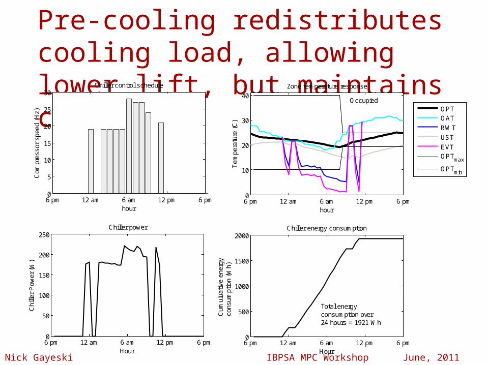
Zone temperature response
6 pm 12 am 6 am 12 pm 6 pm0
500
1000
1500
2000
Hour
Cum
ulua
tive
ener
gy
cons
umpt
ion
(Wh)
Chiller energy consumption
6 pm 12 am 6 am 12 pm 6 pm0
50
100
150
200
250
Hour
Chi
ller
Pow
er (
W)
Chiller power
6 pm 12 am 6 am 12 pm 6 pm0
5
10
15
20
25
30
hour
Com
pres
sor
spee
d (H
z)
Chiller control schedule
OPTOAT
RWT
UST
EVTOPT
max
OPTmin
Total energy consumption over 24 hours = 1921 Wh
Occupied
Nick Gayeski IBPSA MPC Workshop June, 2011
Pre-cooling redistributes cooling load, allowing lower lift, but maintains comfort
6 pm 12 am 6 am 12 pm 6 pm0
10
20
30
40
hour
Tem
pera
ture
(C
)
Zone temperature response
6 pm 12 am 6 am 12 pm 6 pm0
500
1000
1500
2000
Hour
Cum
ulua
tive
ener
gy
cons
umpt
ion
(Wh)
Chiller energy consumption
6 pm 12 am 6 am 12 pm 6 pm0
50
100
150
200
250
Hour
Chi
ller
Pow
er (
W)
Chiller power
6 pm 12 am 6 am 12 pm 6 pm0
5
10
15
20
25
30
hour
Com
pres
sor
spee
d (H
z)
Chiller control schedule
OPTOAT
RWT
UST
EVTOPT
max
OPTmin
Total energy consumption over 24 hours = 1921 Wh
Occupied
Nick Gayeski IBPSA MPC Workshop June, 2011
Comparing experimental results to PNNL simulation studies
Nick Gayeski IBPSA MPC Workshop June, 2011
Select a base-case system as a point of comparison to the PNNL simulation studies.
Low fan energy split-system air conditioner SEER 16 with conventional controls is representative of case with high efficiency distribution, conventional chiller operation
Test base-case subject to the same conditions as the LLCS but with thermostatic control achieving same mean temperature
Compare energy savings in the experimental tests with the PNNL simulations
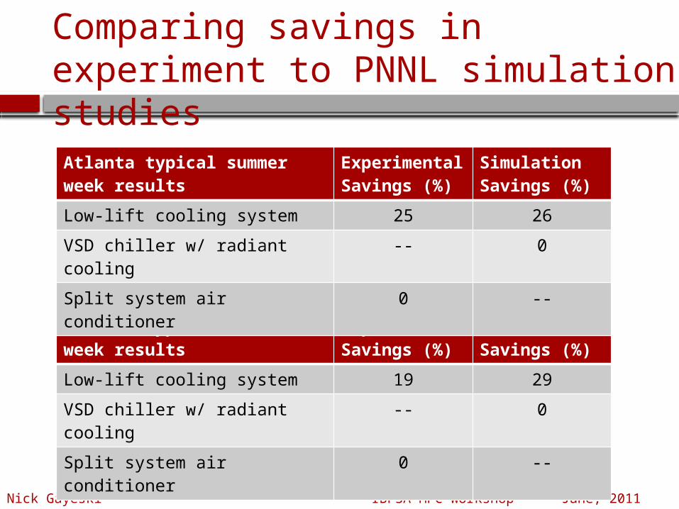
Comparing savings in experiment to PNNL simulation studies
Nick Gayeski IBPSA MPC Workshop June, 2011
Phoenix typical summer week results
Experimental Savings (%)
Simulation Savings (%)
Low-lift cooling system 19 29
VSD chiller w/ radiant cooling -- 0
Split system air conditioner 0 --
Atlanta typical summer week results
Experimental Savings (%)
Simulation Savings (%)
Low-lift cooling system 25 26
VSD chiller w/ radiant cooling -- 0
Split system air conditioner 0 --
Improve TABS design by decreasing chilled water pipe spacing permitting higher evaporating temperatures
Better matching of system capacity and loads using a smaller chiller or adding a false load
Improve chamber insulation to achieve closer to adiabatic boundary conditions
Comparison to more configurations of systems and control scenarios, comparisons to identical simulations
Improvements are likely to yield better LLCS performance
Critiquing the experimental LLCS tests
Nick Gayeski IBPSA MPC Workshop June, 2011
5. Ongoing research
Extend to multi-zone TABS systems where multiple zone temperature and TABS responses are predicted simultaneous
Allow TABS pre-cooling and direct cooling at the same time using radiant ceiling panels or efficient zone sensible cooling
Construct a full-scale demonstration project at Masdar City, Abu Dhabi and a location in the United States
Expand simulations using the Building Control Virtual Test Bed by coupling simulation environments required for TABS response and low-lift chiller simulation
Nick Gayeski IBPSA MPC Workshop June, 2011
Summary
Developed a method for data-driven MPC of low-lift chillers pre-cooling TABS leveraging curve-fit chiller modeling and CRTF zone temperature modeling
Implemented these methods in an experimental test chamber leveraging curve-fit chiller modeling and CRTF zone temperature modeling
Compared performance to a split-system air conditioner as a basis for comparison to predominant technology and to spot-check against PNNL simulations
Nick Gayeski IBPSA MPC Workshop June, 2011
Thank you! Questions welcome
Nicholas Gayeski, PhD
Research Affiliate Partner and Co-FounderMassachusetts Institute of Technology KGS Buildings,
Thank you to my advisors: Prof. Leslie K. Norford, Prof. Peter R. Armstrong, and Prof. Leon Glicksman
Thank you to: Srinivas Katipamula and PNNLMitsubishi Electric Research LaboratoryMartin Family Society of FellowsMassachusetts Institute of TechnologyMasdar Institute of Science and