DAYTIME WATER DETECTION BY FUSING MULTIPLE CUES FOR AUTONOMOUS OFF-ROAD NAVIGATION A. L. Rankin*, L. H. Matthies, and A. Huertas Jet Propulsion Laboratory 4800 Oak Grove Drive, Pasadena, CA, USA 91109 ABSTRACT Detecting water hazards is a significant challenge to unmanned ground vehicle autonomous off-road navigation. This paper focuses on detecting the presence of water during the daytime using color cameras. A multi-cue approach is taken. Evidence of the presence of water is generated from color, texture, and the detection of reflections in stereo range data. A rule base for fusing water cues was developed by evaluating detection results from an extensive archive of data collection imagery containing water. This software has been implemented into a run-time passive perception subsystem and tested thus far under Linux on a Pentium based processor. 1. INTRODUCTION Robust water detection is a critical requirement for autonomous off-road navigation. Traversing through water bodies sufficiently deep can cause damage to non- watertight unmanned ground vehicle (UGV) electronics. In addition, a UGV stuck in a water body during an in- theater autonomous mission may require human intervention in the form of towing, or sacrificing. The large number of possible scenarios and appearances of water makes water detection particularly challenging for visual sensors. Laser sensors, commonly used for UGV autonomous navigation, often get no return value on free- standing water (Hong, 1998) In (Matthies, 2003), we cataloged the environmental variables affecting the difficulty of this problem and discussed the sensors applicable to detecting water hazards under each condition. In this paper, we focus on techniques applicable to detecting water hazards during the daytime using passive sensors, and a strategy for fusing multiple water detection cues into a terrain map, from which a UGV can perform autonomous navigation (Lacaze, 2002). 2. APPROACH The scene in Figure 1 illustrates several appearances of standing water in color imagery: brighter intensities where the sky is reflected, darker intensities where the water is in shadow, and reflections of ground cover that are close and far away. In addition, no leading edge is visible for portions of the closer water body. It is difficult to create a single detector that locates all these features. Here, we take a multi-cue approach. Water cues from color, texture, and stereo range analysis are fused together using a rule base developed by processing 25 archived RGB color stereo image pairs from multiple sites (Ft. Indiantown Gap, PA, Ft. Knox, KY, Ft. Polk, LA, Ft. A. P. Hill, VA, Chatfield State Park, CO, and the Angeles National Forest, CA). This data set has natural scenes contains standing water, moving water, a lake, a large pond, small bodies of water, clear water, turbid water, water under a canopy, and water in the open. An advantage of a multi-cue approach is that each detector can be designed to target a specific water attribute. Perfect detection of an entire water body is thus, not expected by any single detector. The fusion of water cues enhances detection of water bodies with multiple attributes. The rules for fusing the water cues are designed to maximize water body detection while minimizing false detection. In the following section, we discuss water cues from color, texture, and stereo range data. Figure 1. Rectified RGB color image of two large puddles on a road at Ft. Indiantown Gap, PA. 2.1 Water Cue from Color In previous UGV programs (Bulletta, 2000), we have used an RGB color image classifier based on supervised classification with a mixture of Gaussians model to detect sky reflections in water bodies. But the training, which needs to be repeated at each new site of operation using 1
Transcript
DAYTIME WATER DETECTION BY FUSING MULTIPLE CUES FOR AUTONOMOUS OFF-ROAD NAVIGATION
A. L. Rankin*, L. H. Matthies, and A. Huertas Jet Propulsion Laboratory
4800 Oak Grove Drive, Pasadena, CA, USA 91109
ABSTRACT
Detecting water hazards is a significant challenge to unmanned ground vehicle autonomous off-road navigation. This paper focuses on detecting the presence of water during the daytime using color cameras. A multi-cue approach is taken. Evidence of the presence of water is generated from color, texture, and the detection of reflections in stereo range data. A rule base for fusing water cues was developed by evaluating detection results from an extensive archive of data collection imagery containing water. This software has been implemented into a run-time passive perception subsystem and tested thus far under Linux on a Pentium based processor.
1. INTRODUCTION
Robust water detection is a critical requirement for autonomous off-road navigation. Traversing through water bodies sufficiently deep can cause damage to non-watertight unmanned ground vehicle (UGV) electronics. In addition, a UGV stuck in a water body during an in-theater autonomous mission may require human intervention in the form of towing, or sacrificing. The large number of possible scenarios and appearances of water makes water detection particularly challenging for visual sensors. Laser sensors, commonly used for UGV autonomous navigation, often get no return value on free-standing water (Hong, 1998)
In (Matthies, 2003), we cataloged the environmental
variables affecting the difficulty of this problem and discussed the sensors applicable to detecting water hazards under each condition. In this paper, we focus on techniques applicable to detecting water hazards during the daytime using passive sensors, and a strategy for fusing multiple water detection cues into a terrain map, from which a UGV can perform autonomous navigation (Lacaze, 2002).
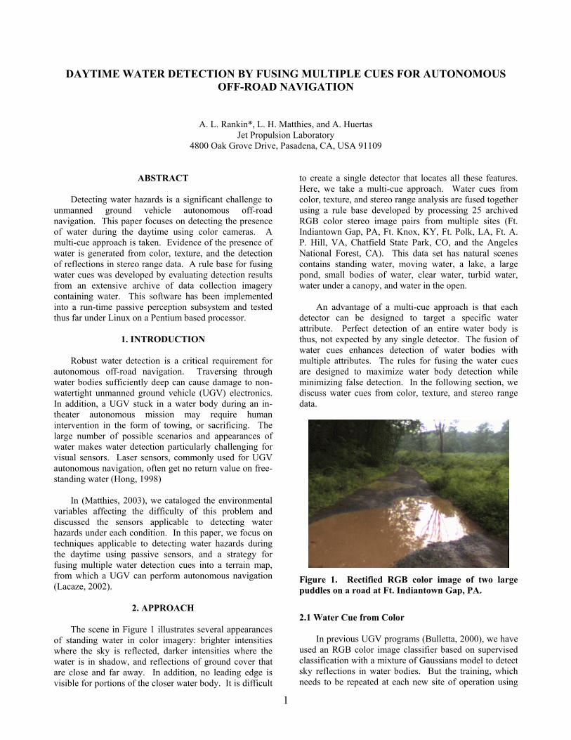
2. APPROACH The scene in Figure 1 illustrates several appearances of standing water in color imagery: brighter intensities where the sky is reflected, darker intensities where the water is in shadow, and reflections of ground cover that are close and far away. In addition, no leading edge is visible for portions of the closer water body. It is difficult
to create a single detector that locates all these features. Here, we take a multi-cue approach. Water cues from color, texture, and stereo range analysis are fused together using a rule base developed by processing 25 archived RGB color stereo image pairs from multiple sites (Ft. Indiantown Gap, PA, Ft. Knox, KY, Ft. Polk, LA, Ft. A. P. Hill, VA, Chatfield State Park, CO, and the Angeles National Forest, CA). This data set has natural scenes contains standing water, moving water, a lake, a large pond, small bodies of water, clear water, turbid water, water under a canopy, and water in the open.
An advantage of a multi-cue approach is that each detector can be designed to target a specific water attribute. Perfect detection of an entire water body is thus, not expected by any single detector. The fusion of water cues enhances detection of water bodies with multiple attributes. The rules for fusing the water cues are designed to maximize water body detection while minimizing false detection. In the following section, we discuss water cues from color, texture, and stereo range data.
Figure 1. Rectified RGB color image of two large puddles on a road at Ft. Indiantown Gap, PA.
2.1 Water Cue from Color In previous UGV programs (Bulletta, 2000), we have used an RGB color image classifier based on supervised classification with a mixture of Gaussians model to detect sky reflections in water bodies. But the training, which needs to be repeated at each new site of operation using
1
representative imagery, is cumbersome. Furthermore, there are times when it is not feasible to take a UGV into the theater of operation to acquire imagery of sample water bodies for training. Here, we attempt to generate thresholding criteria based on an evaluation of a set of images containing water having a variety of appearances.
00.20.40.60.81
0 45 90 135 180 225 270 315 360
Hue (degrees)
Satu
ratio
n
The RGB images selected from our archive for
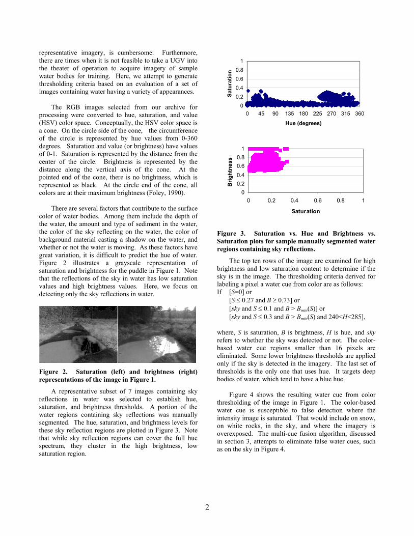
processing were converted to hue, saturation, and value (HSV) color space. Conceptually, the HSV color space is a cone. On the circle side of the cone, the circumference of the circle is represented by hue values from 0-360 degrees. Saturation and value (or brightness) have values of 0-1. Saturation is represented by the distance from the center of the circle. Brightness is represented by the distance along the vertical axis of the cone. At the pointed end of the cone, there is no brightness, which is represented as black. At the circle end of the cone, all colors are at their maximum brightness (Foley, 1990). 0
0.20.40.60.81
0 0.2 0.4 0.6 0.8 1
Saturation
Brig
htne
ss
There are several factors that contribute to the surface
color of water bodies. Among them include the depth of the water, the amount and type of sediment in the water, the color of the sky reflecting on the water, the color of background material casting a shadow on the water, and whether or not the water is moving. As these factors have great variation, it is difficult to predict the hue of water. Figure 2 illustrates a grayscale representation of saturation and brightness for the puddle in Figure 1. Note that the reflections of the sky in water has low saturation values and high brightness values. Here, we focus on detecting only the sky reflections in water.
Figure 3. Saturation vs. Hue and Brightness vs. Saturation plots for sample manually segmented water regions containing sky reflections.
The top ten rows of the image are examined for high brightness and low saturation content to determine if the sky is in the image. The thresholding criteria derived for labeling a pixel a water cue from color are as follows: If [S=0] or
[S ≤ 0.27 and B ≥ 0.73] or [sky and S ≤ 0.1 and B > Bmin(S)] or
[sky and S ≤ 0.3 and B > Bmin(S) and 240<H<285], where, S is saturation, B is brightness, H is hue, and sky refers to whether the sky was detected or not. The color-based water cue regions smaller than 16 pixels are eliminated. Some lower brightness thresholds are applied only if the sky is detected in the imagery. The last set of thresholds is the only one that uses hue. It targets deep bodies of water, which tend to have a blue hue.
Figure 2. Saturation (left) and brightness (right) representations of the image in Figure 1.
A representative subset of 7 images containing sky reflections in water was selected to establish hue, saturation, and brightness thresholds. A portion of the water regions containing sky reflections was manually segmented. The hue, saturation, and brightness levels for these sky reflection regions are plotted in Figure 3. Note that while sky reflection regions can cover the full hue spectrum, they cluster in the high brightness, low saturation region.
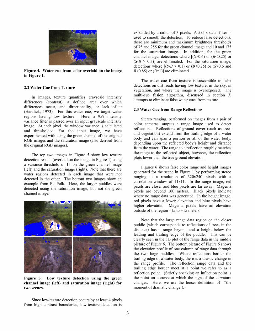
Figure 4 shows the resulting water cue from color thresholding of the image in Figure 1. The color-based water cue is susceptible to false detection where the intensity image is saturated. That would include on snow, on white rocks, in the sky, and where the imagery is overexposed. The multi-cue fusion algorithm, discussed in section 3, attempts to eliminate false water cues, such as on the sky in Figure 4.
2
Figure 4. Water cue from color overlaid on the image in Figure 1.
2.2 Water Cue from Texture In images, texture quantifies grayscale intensity differences (contrast), a defined area over which differences occur, and directionality, or lack of it (Haralick, 1973). For this water cue, we target water regions having low texture. Here, a 9x9 intensity variance filter is passed over an input grayscale intensity image. At each pixel, the window variance is calculated and thresholded. For the input image, we have experimented with using the green channel of the original RGB images and the saturation image (also derived from the original RGB images).
The top two images in Figure 5 show low texture detection results (overlaid on the image in Figure 1) using a variance threshold of 13 on the green channel image (left) and the saturation image (right). Note that there are water regions detected in each image that were not detected in the other. The bottom two images show an example from Ft. Polk. Here, the larger puddles were detected using the saturation image, but not the green channel image.
Figure 5. Low texture detection using the green channel image (left) and saturation image (right) for two scenes.
Since low-texture detection occurs by at least 4 pixels
from high contrast boundaries, low-texture detection is
expanded by a radius of 3 pixels. A 5x5 spacial filter is used to smooth the detection. To reduce false detections, there are minimum and maximum brightness thresholds of 75 and 255 for the green channel image and 10 and 175 for the saturation image. In addition, for the green channel image, detections where [(S>0.6) or (B<0.25) or (S-B > 0.3)] are eliminated. For the saturation image, detections where [(S-B > 0.1) or (B<0.25) or (S>0.6 and B<0.85) or (B=1)] are eliminated.
The water cue from texture is susceptible to false detections on dirt roads having low texture, in the sky, in vegetation, and where the image is overexposed. The multi-cue fusion algorithm, discussed in section 3, attempts to eliminate false water cues from texture. 2.3 Water Cue from Range Reflections
Stereo ranging, performed on images from a pair of color cameras, outputs a range image used to detect reflections. Reflections of ground cover (such as trees and vegetation) extend from the trailing edge of a water body and can span a portion or all of the water body, depending upon the reflected body’s height and distance from the water. The range to a reflection roughly matches the range to the reflected object, however, the reflection plots lower than the true ground elevation.
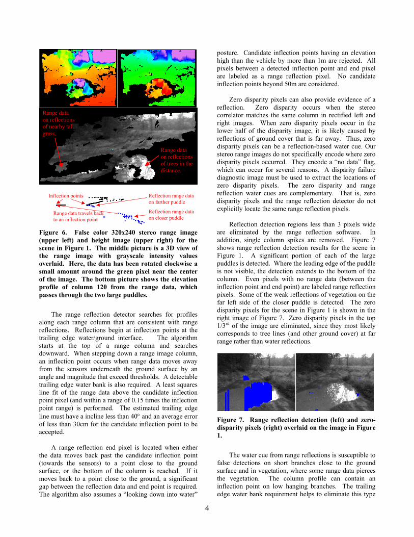
Figures 6 shows false color range and height images
generated for the scene in Figure 1 by performing stereo ranging at a resolution of 320x240 pixels with a correlation window of 11x11. In the range image, red pixels are closer and blue pixels are far away. Magenta pixels are beyond 100 meters. Black pixels indicate where no range data was generated. In the height image, red pixels have a lower elevation and blue pixels have higher elevation. Magenta pixels have an elevation outside of the region –15 to +15 meters.
Note that the large range data region on the closer
puddle (which corresponds to reflections of trees in the distance) has a range beyond and a height below the leading and trailing edge of the puddle. This can be clearly seen in the 3D plot of the range data in the middle picture of Figure 6. The bottom picture of Figure 6 shows the elevation profile of one column of range data through the two large puddles. Where reflections border the trailing edge of a water body, there is a drastic change in the range profile. The reflection range data and the trailing edge border meet at a point we refer to as a reflection point. (Strictly speaking an inflection point is the point on a curve at which the sign of the curvature changes. Here, we use the looser definition of “the moment of dramatic change’).
3
Range data on reflections of trees in the distance.
Range data on reflections of nearby tall grass.
Range data travels back to an inflection point
Reflection range data on closer puddle
Reflection range data on farther puddle
Inflection points
Figure 6. False color 320x240 stereo range image (upper left) and height image (upper right) for the scene in Figure 1. The middle picture is a 3D view of the range image with grayscale intensity values overlaid. Here, the data has been rotated clockwise a small amount around the green pixel near the center of the image. The bottom picture shows the elevation profile of column 120 from the range data, which passes through the two large puddles.
The range reflection detector searches for profiles
along each range column that are consistent with range reflections. Reflections begin at inflection points at the trailing edge water/ground interface. The algorithm starts at the top of a range column and searches downward. When stepping down a range image column, an inflection point occurs when range data moves away from the sensors underneath the ground surface by an angle and magnitude that exceed thresholds. A detectable trailing edge water bank is also required. A least squares line fit of the range data above the candidate inflection point pixel (and within a range of 0.15 times the inflection point range) is performed. The estimated trailing edge line must have a incline less than 40° and an average error of less than 30cm for the candidate inflection point to be accepted.
A range reflection end pixel is located when either
the data moves back past the candidate inflection point (towards the sensors) to a point close to the ground surface, or the bottom of the column is reached. If it moves back to a point close to the ground, a significant gap between the reflection data and end point is required. The algorithm also assumes a “looking down into water”
posture. Candidate inflection points having an elevation high than the vehicle by more than 1m are rejected. All pixels between a detected inflection point and end pixel are labeled as a range reflection pixel. No candidate inflection points beyond 50m are considered.
Zero disparity pixels can also provide evidence of a reflection. Zero disparity occurs when the stereo correlator matches the same column in rectified left and right images. When zero disparity pixels occur in the lower half of the disparity image, it is likely caused by reflections of ground cover that is far away. Thus, zero disparity pixels can be a reflection-based water cue. Our stereo range images do not specifically encode where zero disparity pixels occurred. They encode a “no data” flag, which can occur for several reasons. A disparity failure diagnostic image must be used to extract the locations of zero disparity pixels. The zero disparity and range reflection water cues are complementary. That is, zero disparity pixels and the range reflection detector do not explicitly locate the same range reflection pixels.
Reflection detection regions less than 3 pixels wide
are eliminated by the range reflection software. In addition, single column spikes are removed. Figure 7 shows range reflection detection results for the scene in Figure 1. A significant portion of each of the large puddles is detected. Where the leading edge of the puddle is not visible, the detection extends to the bottom of the column. Even pixels with no range data (between the inflection point and end point) are labeled range reflection pixels. Some of the weak reflections of vegetation on the far left side of the closer puddle is detected. The zero disparity pixels for the scene in Figure 1 is shown in the right image of Figure 7. Zero disparity pixels in the top 1/3rd of the image are eliminated, since they most likely corresponds to tree lines (and other ground cover) at far range rather than water reflections.
Figure 7. Range reflection detection (left) and zero-disparity pixels (right) overlaid on the image in Figure 1.
The water cue from range reflections is susceptible to
false detections on short branches close to the ground surface and in vegetation, where some range data pierces the vegetation. The column profile can contain an inflection point on low hanging branches. The trailing edge water bank requirement helps to eliminate this type
4
of false detection. The multi-cue fusion algorithm, discussed in section 3, attempts to eliminate false water cues from range reflections.
3. FUSING WATER CUES
The water fusion run-time software module currently
merges water cues from a range-reflection detector, an HSV color image sky-reflection detector based on simple thresholding criteria, a low-texture detector that thresholds intensity variance and brightness, and zero disparity pixels obtained from a disparity failure diagnostic image. In addition, any detection above the horizon line or 0.75m above the bottom of the vehicle control point (center of the rear axle at ground height) is eliminated. This eliminates false detections in the sky and tall ground cover.
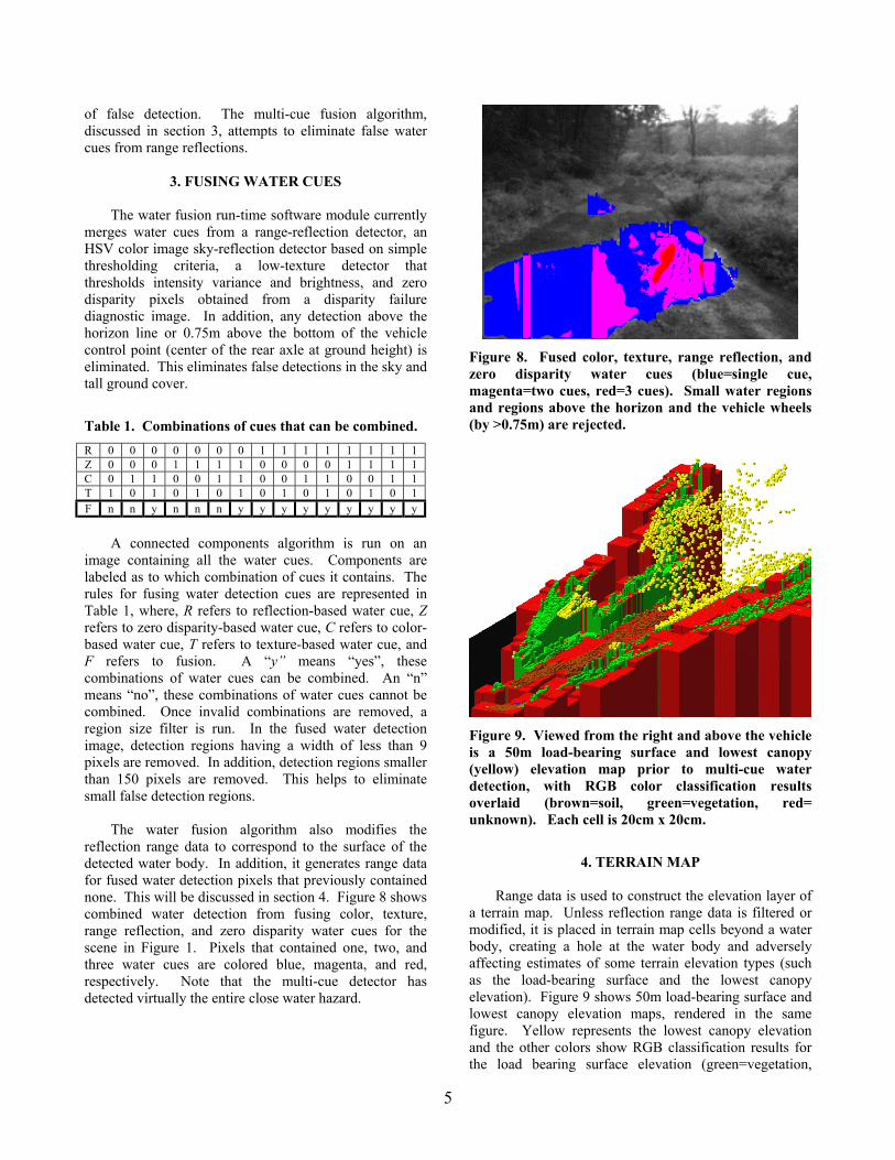
Figure 8. Fused color, texture, range reflection, and zero disparity water cues (blue=single cue, magenta=two cues, red=3 cues). Small water regions and regions above the horizon and the vehicle wheels (by >0.75m) are rejected.
Table 1. Combinations of cues that can be combined. R 0 0 0 0 0 0 0 1 1 1 1 1 1 1 1
Z 0 0 0 1 1 1 1 0 0 0 0 1 1 1 1 C 0 1 1 0 0 1 1 0 0 1 1 0 0 1 1 T 1 0 1 0 1 0 1 0 1 0 1 0 1 0 1 F n n y n n n y y y y y y y y y
A connected components algorithm is run on an
image containing all the water cues. Components are labeled as to which combination of cues it contains. The rules for fusing water detection cues are represented in Table 1, where, R refers to reflection-based water cue, Z refers to zero disparity-based water cue, C refers to color-based water cue, T refers to texture-based water cue, and F refers to fusion. A “y” means “yes”, these combinations of water cues can be combined. An “n” means “no”, these combinations of water cues cannot be combined. Once invalid combinations are removed, a region size filter is run. In the fused water detection image, detection regions having a width of less than 9 pixels are removed. In addition, detection regions smaller than 150 pixels are removed. This helps to eliminate small false detection regions.
Figure 9. Viewed from the right and above the vehicle is a 50m load-bearing surface and lowest canopy (yellow) elevation map prior to multi-cue water detection, with RGB color classification results overlaid (brown=soil, green=vegetation, red= unknown). Each cell is 20cm x 20cm.
The water fusion algorithm also modifies the reflection range data to correspond to the surface of the detected water body. In addition, it generates range data for fused water detection pixels that previously contained none. This will be discussed in section 4. Figure 8 shows combined water detection from fusing color, texture, range reflection, and zero disparity water cues for the scene in Figure 1. Pixels that contained one, two, and three water cues are colored blue, magenta, and red, respectively. Note that the multi-cue detector has detected virtually the entire close water hazard.
4. TERRAIN MAP
Range data is used to construct the elevation layer of
a terrain map. Unless reflection range data is filtered or modified, it is placed in terrain map cells beyond a water body, creating a hole at the water body and adversely affecting estimates of some terrain elevation types (such as the load-bearing surface and the lowest canopy elevation). Figure 9 shows 50m load-bearing surface and lowest canopy elevation maps, rendered in the same figure. Yellow represents the lowest canopy elevation and the other colors show RGB classification results for the load bearing surface elevation (green=vegetation,
5
brown=soil, red=unknown). At range, a portion of the road is corrupted by reflection range data (which has a lower elevation). The minimum canopy elevation is corrupted as well by range data that really belongs to the ground cover.
Inflection points
Puddles
75m 30m
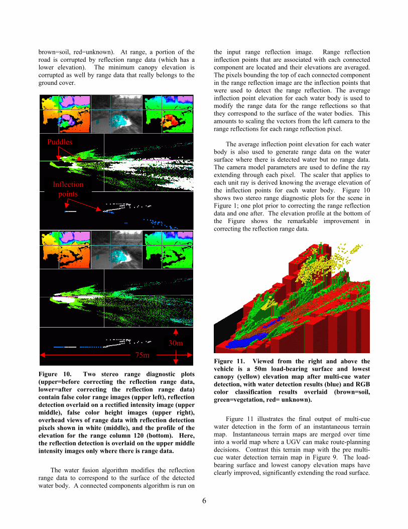
Figure 10. Two stereo range diagnostic plots (upper=before correcting the reflection range data, lower=after correcting the reflection range data) contain false color range images (upper left), reflection detection overlaid on a rectified intensity image (upper middle), false color height images (upper right), overhead views of range data with reflection detection pixels shown in white (middle), and the profile of the elevation for the range column 120 (bottom). Here, the reflection detection is overlaid on the upper middle intensity images only where there is range data.
The water fusion algorithm modifies the reflection
range data to correspond to the surface of the detected water body. A connected components algorithm is run on
the input range reflection image. Range reflection inflection points that are associated with each connected component are located and their elevations are averaged. The pixels bounding the top of each connected component in the range reflection image are the inflection points that were used to detect the range reflection. The average inflection point elevation for each water body is used to modify the range data for the range reflections so that they correspond to the surface of the water bodies. This amounts to scaling the vectors from the left camera to the range reflections for each range reflection pixel.
The average inflection point elevation for each water
body is also used to generate range data on the water surface where there is detected water but no range data. The camera model parameters are used to define the ray extending through each pixel. The scaler that applies to each unit ray is derived knowing the average elevation of the inflection points for each water body. Figure 10 shows two stereo range diagnostic plots for the scene in Figure 1; one plot prior to correcting the range reflection data and one after. The elevation profile at the bottom of the Figure shows the remarkable improvement in correcting the reflection range data.
Figure 11. Viewed from the right and above the vehicle is a 50m load-bearing surface and lowest canopy (yellow) elevation map after multi-cue water detection, with water detection results (blue) and RGB color classification results overlaid (brown=soil, green=vegetation, red= unknown).
Figure 11 illustrates the final output of multi-cue
water detection in the form of an instantaneous terrain map. Instantaneous terrain maps are merged over time into a world map where a UGV can make route-planning decisions. Contrast this terrain map with the pre multi-cue water detection terrain map in Figure 9. The load-bearing surface and lowest canopy elevation maps have clearly improved, significantly extending the road surface.
6
5. OTHER RESULTS
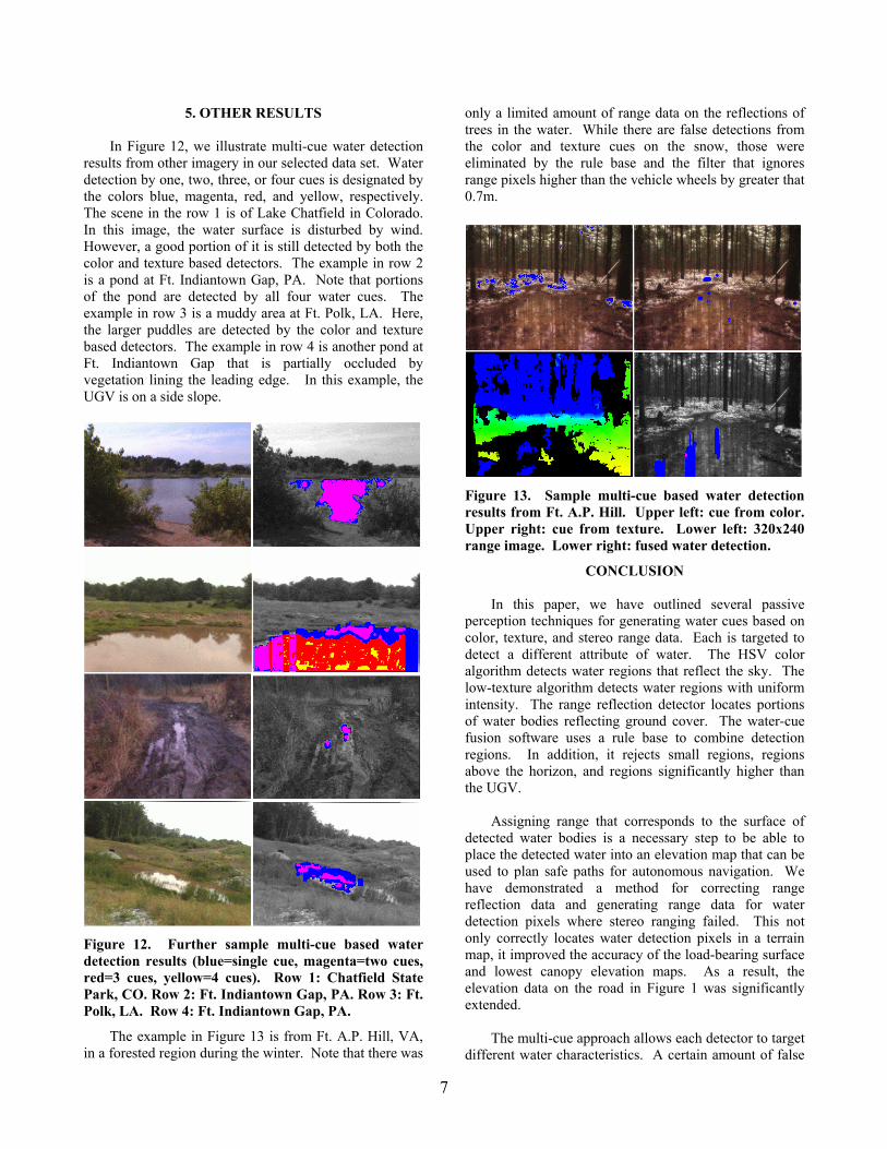
In Figure 12, we illustrate multi-cue water detection results from other imagery in our selected data set. Water detection by one, two, three, or four cues is designated by the colors blue, magenta, red, and yellow, respectively. The scene in the row 1 is of Lake Chatfield in Colorado. In this image, the water surface is disturbed by wind. However, a good portion of it is still detected by both the color and texture based detectors. The example in row 2 is a pond at Ft. Indiantown Gap, PA. Note that portions of the pond are detected by all four water cues. The example in row 3 is a muddy area at Ft. Polk, LA. Here, the larger puddles are detected by the color and texture based detectors. The example in row 4 is another pond at Ft. Indiantown Gap that is partially occluded by vegetation lining the leading edge. In this example, the UGV is on a side slope.
Figure 12. Further sample multi-cue based water detection results (blue=single cue, magenta=two cues, red=3 cues, yellow=4 cues). Row 1: Chatfield State Park, CO. Row 2: Ft. Indiantown Gap, PA. Row 3: Ft. Polk, LA. Row 4: Ft. Indiantown Gap, PA.
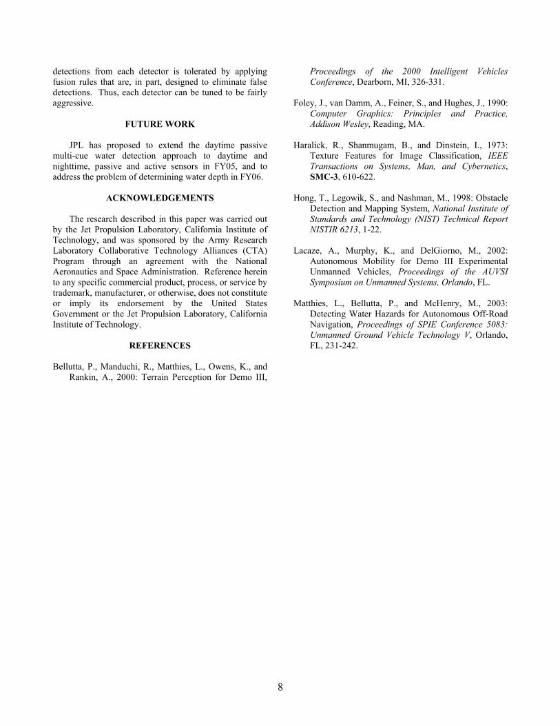
The example in Figure 13 is from Ft. A.P. Hill, VA, in a forested region during the winter. Note that there was
only a limited amount of range data on the reflections of trees in the water. While there are false detections from the color and texture cues on the snow, those were eliminated by the rule base and the filter that ignores range pixels higher than the vehicle wheels by greater that 0.7m.
Figure 13. Sample multi-cue based water detection results from Ft. A.P. Hill. Upper left: cue from color. Upper right: cue from texture. Lower left: 320x240 range image. Lower right: fused water detection.
CONCLUSION
In this paper, we have outlined several passive perception techniques for generating water cues based on color, texture, and stereo range data. Each is targeted to detect a different attribute of water. The HSV color algorithm detects water regions that reflect the sky. The low-texture algorithm detects water regions with uniform intensity. The range reflection detector locates portions of water bodies reflecting ground cover. The water-cue fusion software uses a rule base to combine detection regions. In addition, it rejects small regions, regions above the horizon, and regions significantly higher than the UGV.
Assigning range that corresponds to the surface of detected water bodies is a necessary step to be able to place the detected water into an elevation map that can be used to plan safe paths for autonomous navigation. We have demonstrated a method for correcting range reflection data and generating range data for water detection pixels where stereo ranging failed. This not only correctly locates water detection pixels in a terrain map, it improved the accuracy of the load-bearing surface and lowest canopy elevation maps. As a result, the elevation data on the road in Figure 1 was significantly extended.
The multi-cue approach allows each detector to target
different water characteristics. A certain amount of false
7
detections from each detector is tolerated by applying fusion rules that are, in part, designed to eliminate false detections. Thus, each detector can be tuned to be fairly aggressive.
FUTURE WORK JPL has proposed to extend the daytime passive multi-cue water detection approach to daytime and nighttime, passive and active sensors in FY05, and to address the problem of determining water depth in FY06.
ACKNOWLEDGEMENTS
The research described in this paper was carried out by the Jet Propulsion Laboratory, California Institute of Technology, and was sponsored by the Army Research Laboratory Collaborative Technology Alliances (CTA) Program through an agreement with the National Aeronautics and Space Administration. Reference herein to any specific commercial product, process, or service by trademark, manufacturer, or otherwise, does not constitute or imply its endorsement by the United States Government or the Jet Propulsion Laboratory, California Institute of Technology.
REFERENCES Bellutta, P., Manduchi, R., Matthies, L., Owens, K., and
Rankin, A., 2000: Terrain Perception for Demo III,
Proceedings of the 2000 Intelligent Vehicles Conference, Dearborn, MI, 326-331.
Foley, J., van Damm, A., Feiner, S., and Hughes, J., 1990:
Computer Graphics: Principles and Practice, Addison Wesley, Reading, MA.
Haralick, R., Shanmugam, B., and Dinstein, I., 1973:
Texture Features for Image Classification, IEEE Transactions on Systems, Man, and Cybernetics, SMC-3, 610-622.
Hong, T., Legowik, S., and Nashman, M., 1998: Obstacle
Detection and Mapping System, National Institute of Standards and Technology (NIST) Technical Report NISTIR 6213, 1-22.
Lacaze, A., Murphy, K., and DelGiorno, M., 2002:
Autonomous Mobility for Demo III Experimental Unmanned Vehicles, Proceedings of the AUVSI Symposium on Unmanned Systems, Orlando, FL.
Matthies, L., Bellutta, P., and McHenry, M., 2003:
Detecting Water Hazards for Autonomous Off-Road Navigation, Proceedings of SPIE Conference 5083: Unmanned Ground Vehicle Technology V, Orlando, FL, 231-242.