2010/47

■

A multilevel approach for nonnegative matrix factorization

Nicolas Gillis and François Glineur

Center for Operations Research and Econometrics

Voie du Roman Pays, 34

B-1348 Louvain-la-Neuve Belgium

http://www.uclouvain.be/core

D I S C U S S I O N P A P E R

CORE DISCUSSION PAPER 2010/47

A multilevel approach

for nonnegative matrix factorization

Nicolas GILLIS 1 and François GLINEUR2

July 2010

Abstract

Nonnegative Matrix Factorization (NMF) is the problem of approximating a nonnegative matrix with the product of two low-rank nonnegative matrices and has been shown to be particularly useful in many applications, e.g., in text mining, image processing, computational biology, etc. In this paper, we explain how algorithms for NMF can be embedded into the framework of multi-level methods in order to accelerate their convergence. This technique can be applied in situations where data admit a good approximate representation in a lower dimensional space through linear transformations preserving nonnegativity. A simple multilevel strategy is described and is experi-mentally shown to speed up significantly three popular NMF algorithms (alternating nonnegative least squares, multiplicative updates and hierarchical alternating least squares) on several standard image datasets. Keywords: nonnegative matrix factorization, algorithms, multigrid and multilevel methods, image processing.

1 Université catholique de Louvain, CORE, B-1348 Louvain-la-Neuve, Belgium. E-mail: Nicolas.gillis@uclouvain.be 2 Université catholique de Louvain, CORE, B-1348 Louvain-la-Neuve, Belgium. E-mail: francois.glineur@uclouvain.be. This author is also member of ECORE, the association between CORE and ECARES.

We thank Quentin Rentmeesters for his helpful comments.

The first author is a research fellow of the Fonds de la Recherche Scientifique (F.R.S.-FNRS).

This paper presents research results of the Belgian Program on Interuniversity Poles of Attraction initiated by the Belgian State, Prime Minister's Office, Science Policy Programming. The scientific responsibility is assumed by the authors.

1 Introduction

Nonnegative Matrix Factorization (NMF) consists in approximating a nonnegative matrix as theproduct of two low-rank nonnegative matrices [26, 22]. More precisely, given a nonnegative matrix Mof dimensions m×n and a factorization rank r, we would like to find two nonnegative matrices V andW with dimensions m× r and r × n such that

M ≈ V W.

This decomposition can be interpreted as follows: denoting by M:j the jth column of M , by V:k thekth column of V and by Wkj the entry of W located at position (k, j), we want

M:j ≈r

∑

k=1

Wkj V:k, Wkj ≥ 0, 1 ≤ j ≤ n,

so that each given (nonnegative) vector M:j is approximated by a nonnegative linear combination of rbasis elements V:k to be found. Nonnegatity of vectors V:k ensures that these basis elements belong tothe same space R

m+ as the columns of M and can then be interpreted in the same way. Moreover, the

additive reconstruction due to nonnegativity of coefficients Wkj leads to a part-based representation

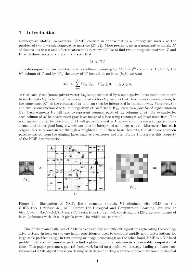
[22]: basis elements V:k will tend to represent common parts of the columns of M . For example, leteach column of M be a vectorized gray-level image of a face using (nonnegative) pixel intensities. Thenonnegative matrix factorization of M will generate a matrix V whose columns are nonnegative basiselements of the original images which can then be interpreted as images as well. Moreover, since eachoriginal face is reconstructed through a weighted sum of these basis elements, the latter are commonparts extracted from the original faces, such as eyes, noses and lips. Figure 1 illustrates this propertyof the NMF decomposition.

Figure 1: Illustration of NMF. Basis elements (matrix V ) obtained with NMF on theCBCL Face Database #1, MIT Center For Biological and Computation Learning, available athttp://cbcl.mit.edu/cbcl/software-datasets/FaceData2.html, consisting of 2429 gray-level images offaces (columns) with 19× 19 pixels (rows) for which we set r = 49.

One of the main challenges of NMF is to design fast and efficient algorithms generating the nonneg-ative factors. In fact, on the one hand, practitioners need to compute rapidly good factorizations forlarge-scale problems (e.g., in text mining or image processing); on the other hand, NMF is a NP-hardproblem [32] and we cannot expect to find a globally optimal solution in a reasonable computationaltime. This paper presents a general framework based on a multilevel strategy leading to faster con-vergence of NMF algorithms when dealing with data admitting a simple approximate low-dimensional

1

representation (using linear transformations preserving nonnegativity), such as images. In fact, inthese situations, a hierarchy of lower-dimensional problems can be constructed and used to computeefficiently approximate solutions of the original problem. Similar techniques have already been usedfor other dimensionality reduction tasks such as PCA [28].

The paper is organized as follows: NMF is first formulated as an optimization problem and threewell-known algorithms (ANLS, MU and HALS) are briefly presented. We then introduce the conceptof multigrid/multilevel methods and show how and why it can be used to speed up NMF algorithms.Finally, we experimentally demonstrate the usefulness of this approach on several standard imagedatabases.

2 Algorithms for NMF

NMF is typically formulated as a nonlinear optimization problem with an objective function measuringthe quality of the low-rank approximation. In this paper, we consider the sum of squared errors:

minV ∈ R

m×r

W ∈ Rr×n

||M − V W ||2F s.t. V ≥ 0, W ≥ 0, (NMF)

i.e., use the squared Frobenius norm ||A||2F =∑

i,j A2ij of the approximation error. Since (NMF)

is NP-hard [32], most NMF algorithms focus on finding locally optimal solutions. In general, onlyconvergence to stationary points of (NMF) (points satisfying the necessary first-order optimalityconditions) is guaranteed.

2.1 Alternating Nonnegative Least Squares (ANLS)

Although (NMF) is a nonconvex problem, it is convex separately in each of the two factors V andW , i.e., finding the optimal factor V corresponding to a fixed factor W reduces to a convex optimiza-tion problem, and vice-versa. More precisely, this convex problem corresponds to a nonnegative leastsquares (NNLS) problem, i.e., a least squares problem with nonnegativity constraints. The so-calledalternating nonnegative least squares (ANLS) algorithm for (NMF) minimizes (exactly) the cost func-tion alternatively over factors V and W so that a stationary point of (NMF) is obtained in the limit[20]. A frequent strategy to solve the NNLS subproblems is to use active set methods [21] (see

Algorithm 1 Alternating Nonnegative Least Squares

Require: Data matrix M ∈ Rm×n+ and initial iterate W ∈ R

r×n+ .

1: while stopping criterion not met do2: V ← argminV ≥0||M − V W ||2F ;3: W ← argminW≥0||M − V W ||2F .4: end while

Appendix A) for which an efficient implementation1 is described in [31, 20]. We refer the reader to [6]for a survey about NNLS methods.

2.2 Multiplicative Updates (MU)

In [23] Lee and Seung propose multiplicative updates (MU) for (NMF) which guarantee nonincreas-ingness of the objective function (cf. Algorithm 2). They also alternatively update V for W fixed andvice versa, using an technique which was originally proposed by Daube-Witherspoon and Muehllehner

2

Algorithm 2 Multiplicative Updates

Require: Data matrix M ∈ Rm×n+ and initial iterates (V,W ) ∈ R

m×r+ × R

r×n+ .

1: while stopping criterion not met do

2: V ← V ◦ [MW T ][V (WW T )]

;

3: W ←W ◦ [V T M ][(V T V )W ]

.

4: end while[.][.] denotes the Hadamard (component-wise) division.

to solve nonnegative least squares problems [13]. The popularity of this algorithm came along withthe popularity of NMF. Algorithm 2 does not guarantee convergence to a stationary point (althoughit can be slightly modified in order to get this property [24, 15]) and it has been observed to convergerelatively very slowly, see [18] and references therein.

2.3 Hierarchical Alternating Least Squares (HALS)

In ANLS, variables are partitioned at each iteration such that each subproblem is convex. However,the resolution of these convex NNLS subproblems is nontrivial and relatively expensive. If we optimizeinstead one single variable at a time, we get a simple univariate quadratic problem which admits aclosed-form solution. Moreover, since the optimal value of each entry of V (resp. W ) does not dependof the other entries of the same column (resp. row), one can optimize alternatively whole columns of Vand whole rows of W . This method was first proposed by Cichocki et al. [10, 8] and independently by[19, 16], and is herein referred to as Hierarchical Alternating Least Squares (HALS), see Algorithm 3.Under some mild assumptions, every limit point is a stationary point of (NMF) [19].

Algorithm 3 Hierarchical Alternating Least Squares

Require: Data M ∈ Rm×n+ and initial iterates (V,W ) ∈ R

m×r+ × R

r×n+ .

1: while stopping criterion not met do2: Compute A = MW T and B = WW T .3: for k = 1 : r do

4: V:k ← max(

0,A:k−

∑rl=1,l6=k V:lBlk

Bkk

)

;

5: end for6: Compute C = V T M and D = V T V .7: for k = 1 : r do

8: Wk: ← max(

0,Ck:−

∑rl=1,l6=k DklWl:

Dkk

)

;

9: end for10: end while

3 Multigrid Methods

In this section, we briefly introduce multigrid methods. The aim is to give the reader some insight onthese techniques in order to comprehend their applications for NMF. We refer the reader to [3, 4, 5, 30]and references therein for detailed discussions on the subject.

1Available at http://www.cc.gatech.edu/~hpark/.

3

Multigrid methods were initially used to develop fast numerical solvers for boundary value prob-lems. Given a differential equation on a continuous domain with boundary conditions, the aim is tofind an approximation of a smooth function f satisfying the constraints. In general, the first step isto discretize the continuous domain, i.e., choose a set of points (a grid) where the function values willbe approximated. Then, a numerical method (e.g., finite differences, finite elements) translates thecontinuous problem into a (square) system of linear equations:

find x ∈ Rn s.t. Ax = b, with A ∈ R

n×n, b ∈ Rn, (3.1)

where the vector x will contain the approximate values of f on the grid points. Linear system (3.1)can be solved either by direct methods (e.g., Gaussian elimination) or iterative methods (e.g., Jacobiand Gauss-Seidel iterations). Of course, the computational cost of these methods depends on thenumber of points in the grid, which leads to a trade-off between precision (number of points used forthe discretization) and computational cost.

Iterative methods update the solution at each step and hopefully converge to a solution of (3.1).Here comes the utility of multigrid: instead of working on a fine grid during all iterations, the solutionis initially restricted to a coarser grid on which the iterations are cheaper. Moreover, the smoothnessof function f allows to recover its low-frequency components faster on coarser grids. Solutions ofthe coarse grid are then prolongated to the finer grid and iterations can continue (higher frequencycomponents of the error are reduced faster). Because the initial guess generated on the coarser gridis (hopefully) a good approximation of the final solution, less iterations are needed on the fine (ex-pensive) grid to converge. Essentially, multigrid methods make iterative methods more efficient, i.e.,accurate solutions are obtained faster.

More recently, these same ideas have been applied to a broader class of problems, e.g., multiscaleoptimization with trust-region methods [17] and multiresolution techniques in image processing [29].

4 Multilevel Approach for NMF

The three algorithms presented in Section 2 (ANLS, MU and HALS) are iteratively trying to find astationary point of (NMF). Actually, most practical NMF algorithms are iterative methods, such asprojected gradient methods [25], Newton-like methods [9, 14], . . . (see also [1, 7, 11, 19] and referencestherein). In order to embed these algorithms in a multilevel strategy, one has to define the differentlevels and describe how the variables and the data are transfered between them. In this section, ageneral description of the multilevel approach for NMF algorithms is first presented and then appliedon image datasets.

4.1 Description

Let each column of the matrix M be a element of the dataset (e.g., a vectorized image) belonging toR

m+ . We define the restriction operator R as a linear operator

R : Rm+ → R

m′

+ : x→R(x) = Rx,

with R ∈ Rm′×m+ and m′ < m; and the prolongation P as a linear operator

P : Rm′

+ → Rm+ : y → P(y) = Py,

with P ∈ Rm×m′

+ . Nonnegativity of matrices R and P is a sufficient condition to preserve nonnegativityof the solutions when they are transfered from one level to another. In fact, in order to generate

4

nonnegative solutions, one requires

R(x) ≥ 0, ∀x ≥ 0 and P(y) ≥ 0, ∀y ≥ 0.

We also define the corresponding transfer operators on matrices, operating columnwise:

R([x1 x2 . . . xn]) = [R(x1)R(x2) . . .R(xn)], and

P([y1 y2 . . . yn]) = [P(y1)P(y2) . . .P(yn)],

for xi ∈ Rm+ , yi ∈ R

m′

+ , 1 ≤ i ≤ n.

In order for the multilevel strategy to work, the information lost when transferring from one levelto another must be limited, i.e., the data matrix M has to be well represented by R(M) in the lowerdimensional space, which means that the reconstruction P(R(M)) must be close to M . From now on,we say that M is smooth with respect to R and P if and only if

sM =||M − P(R(M))||F

||M ||Fis small .

sM gives a measure of how well M can be mapped by R into a lower-dimensional space and thenbrought back by P, and still be a fairly good approximation of itself.

Based on these definitions, elaborating a multilevel approach for NMF is straightforward:

1. We are given M ∈ Rm×n+ and (V0,W0) ∈ R

m×r+ × R

r×n+ ;

2. Compute M ′ = R(M) = RM ∈ Rm′×n+ and V ′

0 = R(V0) = RV0 ∈ Rm′×r+ , i.e., restrict the

elements of your dataset and the basis elements of the current solution to a lower dimensionalspace;

3. Compute a rank-r NMF (V ′,W ) of M ′ using (V ′0 ,W0) as initial matrices, i.e.,

V ′W ≈M ′ = R(M).

This can be done using any NMF iterative algorithm or, even better, using the multilevel strategyrecursively (cf. Section 4.3).

4. SinceM ≈ P(R(M)) = P(M ′) ≈ P(V ′W ) = PV ′W = P(V ′)W = V W,

where V is the prolongation of V ′, (V,W ) is a good initial estimate for a rank-r NMF of M ,provided that M is smooth with respect to R and P (i.e., sM is small) and that V ′W is a goodapproximation of M ′ = R(M) (i.e., ||M ′ − V ′W ||F is small); in fact,

||M − P(V ′)W ||F ≤ ||M − P(R(M))||F + ||P(R(M)) − P(V ′W )||F

≤ sM ||M ||F + ||P(R(M) − V ′W )||F

≤ sM ||M ||F + ||P ||F ||R(M)− V ′W ||F .

5. Further improve the solution (V,W ) using any NMF iterative algorithm.

5

Because computations needed at step 3 are cheap since m′ < m, and in addition the low-frequencycomponents of the error2 is reduced faster on coarse levels (cf. Section 4.4), this strategy will acceleratethe convergence of NMF algorithms.

We now illustrate this technique on image datasets, more precisely, on two-dimensional gray-levelimages. In general, images are composed of several smooth components, i.e., regions where pixelvalues are similar and change continuously with respect to their location (e.g., skin on a face or, thepupil or sclera3 of an eye), that is, a pixel value can often be approximated using the pixel values ofits neighbors. This observation can be used to define the transfer operators (Section 4.2). For thecomputation of a NMF solution needed at step 3, the multilevel approach can be used recursively;three strategies (called multigrid cycles) are described in Section 4.3. Finally, numerical results arereported in Section 5.

4.2 Coarse Grid and Transfer Operators

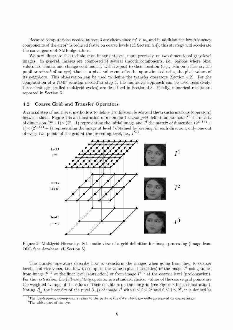
A crucial step of multilevel methods is to define the different levels and the transformations (operators)between them. Figure 2 is an illustration of a standard coarse grid definition: we note I1 the matrixof dimension (2a +1)× (2b +1) representing the initial image and I l the matrix of dimension (2a−l+1 +1)× (2b−l+1 + 1) representing the image at level l obtained by keeping, in each direction, only one outof every two points of the grid at the preceding level, i.e., I l−1.

Figure 2: Multigrid Hierarchy. Schematic view of a grid definition for image processing (image fromORL face database, cf. Section 5).

The transfer operators describe how to transform the images when going from finer to coarserlevels, and vice versa, i.e., how to compute the values (pixel intensities) of the image I l using valuesfrom image I l−1 at the finer level (restriction) or from image I l+1 at the coarser level (prolongation).For the restriction, the full-weighting operator is a standard choice: values of the coarse grid points arethe weighted average of the values of their neighbors on the fine grid (see Figure 3 for an illustration).Noting I l

i,j the intensity of the pixel (i, j) of image I l with 0 ≤ i ≤ 2a and 0 ≤ j ≤ 2b, it is defined as

2The low-frequency components refers to the parts of the data which are well-represented on coarse levels.3The white part of the eye.

6

Figure 3: Restriction and Prolongation.

follows:

I l+1i,j =

1

16

[

I l2i−1,2j−1 + I l

2i−1,2j+1 + I l2i+1,2j−1 + I l

2i+1,2j+1

+ 2(I l2i,2j−1 + I l

2i−1,2j + I l2i+1,2j + I l

2i,2j+1) (4.1)

+ 4I l2i,2j

]

,

except on the boundaries of the image (when i = 0, j = 0, i = 2a and/or j = 2b) where the weightsare adapted correspondingly. For example, to restrict a 3× 3 image to a 2× 2, R is defined with

R =1

9

4 2 0 2 1 0 0 0 00 2 4 0 1 2 0 0 00 0 0 2 1 0 4 2 00 0 0 0 1 2 0 2 4

,

(3 × 3 images needing first to be vectorized to vectors in R9, by concatenation of either columns or

rows).For the prolongation, we set the values on the fine grid points as the average of the values of their

neighbors on the coarse grid:

I li,j = meani′∈rd(i/2)

j′∈rd(j/2)

(

I l+1i′,j′

)

, (4.2)

where

rd(k/2) =

{

{k/2} k even,{(k − 1)/2, (k + 1)/2} k odd.

For example, to prolongate a 2× 2 image to a 3× 3, P is defined with

P T =1

4

4 2 0 2 1 0 0 0 00 2 4 0 1 2 0 0 00 0 0 2 1 0 4 2 00 0 0 0 1 2 0 2 4

.

Note that these transformations clearly preserve nonnegativity.

4.3 Multigrid Cycle

Now that grids and transfer operators are defined, we need to choose the procedure that is appliedat each grid level as it moves through the grid hierarchy. In this section, we propose three differentapproaches: nested iteration, V-cycle and full multigrid cycle.

In our settings, the transfer operators only change the number of rows m of the input matrix M ,i.e., the number of pixels in the images of the database: the size of the images are approximatively

7

four times smaller between each level: m′ ≈ 14m. Since the computational complexity per iteration

of the three algorithms (ANLS, MU and HALS) is almost proportional to m (cf. Appendix A), theiterations will be approximately four times cheaper. A possible way to allocate the time spent ateach level is to allow the same number of iterations at each level, which seems to give good results inpractice. Table 1 shows the time spent and the corresponding number of iterations performed at eachlevel.

Table 1: Number of iterations performed and time spent at each level when allocating among L levelsa total computational budget T corresponding to 4k iterations at the finest level.

Level 1 Level 2 . . . Level L− 1 Level L Total

(finer) . . . (coarser)

∼ # iterations 3k 3k . . . 3k 4k (3L + 1)k

time 34T 3

16T . . . 34L-1 T 1

4L-1 T T

Note that the transfer operators require O(mn) operations and since they are only performed oncebetween each level, their computational cost can be neglected (at least for r ≫ 1 and/or when asizeable amount of iterations are performed).

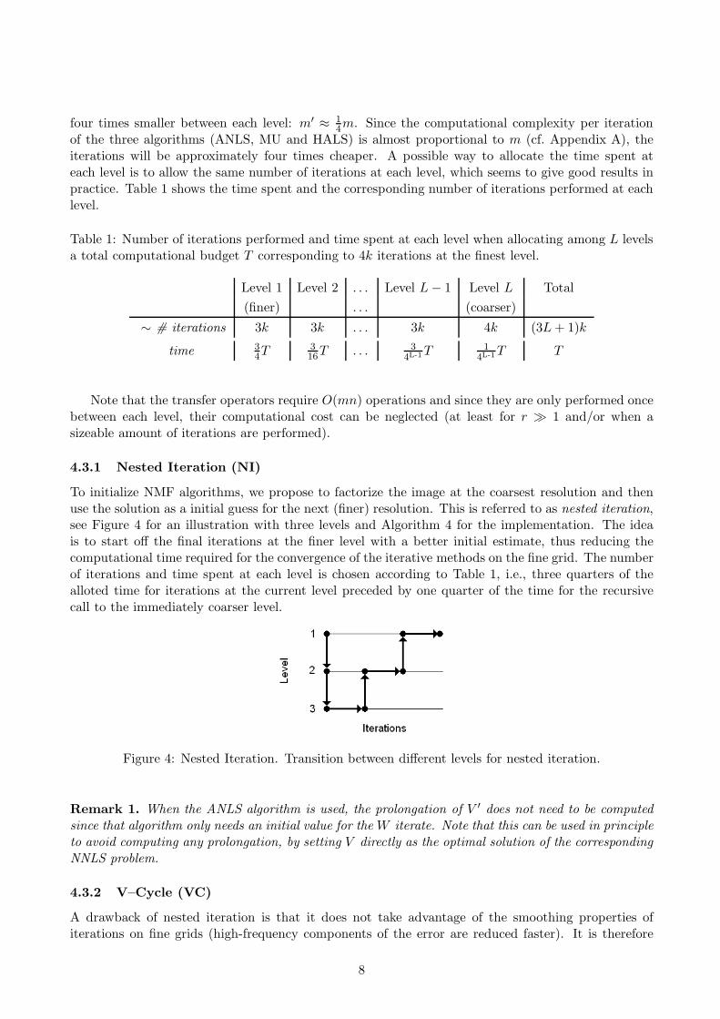
4.3.1 Nested Iteration (NI)

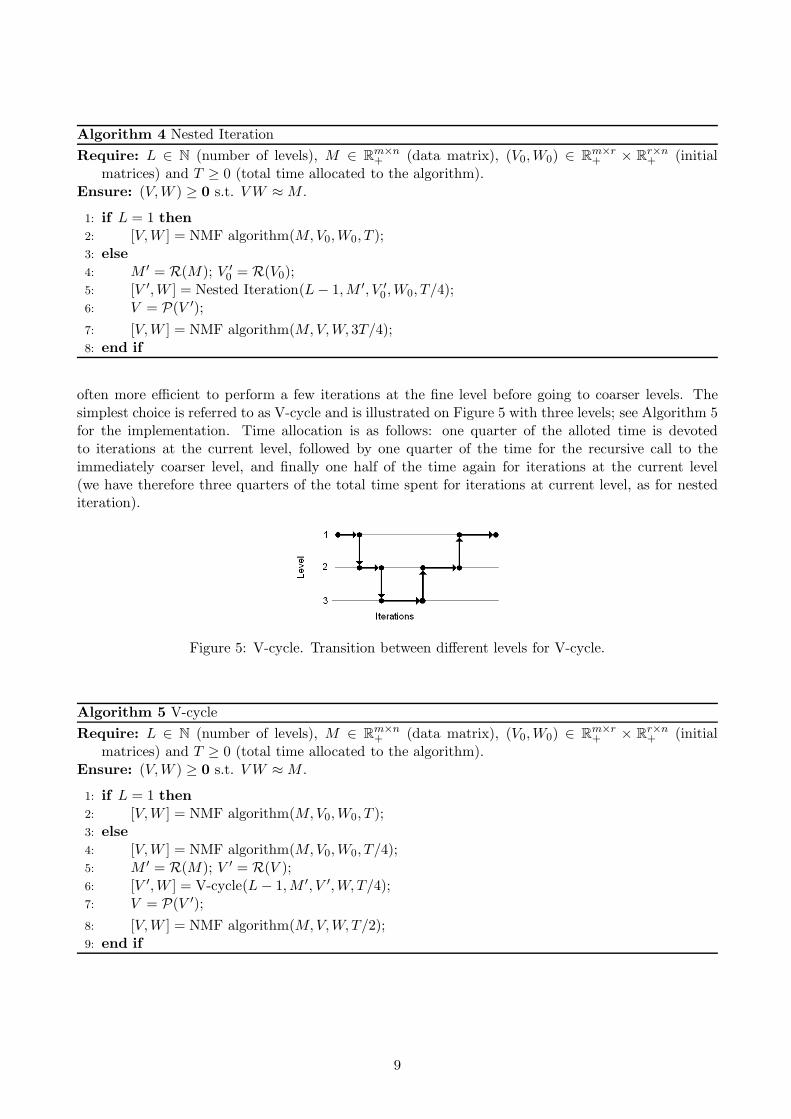
To initialize NMF algorithms, we propose to factorize the image at the coarsest resolution and thenuse the solution as a initial guess for the next (finer) resolution. This is referred to as nested iteration,see Figure 4 for an illustration with three levels and Algorithm 4 for the implementation. The ideais to start off the final iterations at the finer level with a better initial estimate, thus reducing thecomputational time required for the convergence of the iterative methods on the fine grid. The numberof iterations and time spent at each level is chosen according to Table 1, i.e., three quarters of thealloted time for iterations at the current level preceded by one quarter of the time for the recursivecall to the immediately coarser level.

Figure 4: Nested Iteration. Transition between different levels for nested iteration.

Remark 1. When the ANLS algorithm is used, the prolongation of V ′ does not need to be computed

since that algorithm only needs an initial value for the W iterate. Note that this can be used in principle

to avoid computing any prolongation, by setting V directly as the optimal solution of the corresponding

NNLS problem.

4.3.2 V–Cycle (VC)

A drawback of nested iteration is that it does not take advantage of the smoothing properties ofiterations on fine grids (high-frequency components of the error are reduced faster). It is therefore

8

Algorithm 4 Nested Iteration

Require: L ∈ N (number of levels), M ∈ Rm×n+ (data matrix), (V0,W0) ∈ R

m×r+ × R

r×n+ (initial

matrices) and T ≥ 0 (total time allocated to the algorithm).Ensure: (V,W ) ≥ 0 s.t. V W ≈M .

1: if L = 1 then2: [V,W ] = NMF algorithm(M,V0,W0, T );3: else4: M ′ = R(M); V ′

0 = R(V0);5: [V ′,W ] = Nested Iteration(L− 1,M ′, V ′

0 ,W0, T/4);6: V = P(V ′);

7: [V,W ] = NMF algorithm(M,V,W, 3T/4);8: end if

often more efficient to perform a few iterations at the fine level before going to coarser levels. Thesimplest choice is referred to as V-cycle and is illustrated on Figure 5 with three levels; see Algorithm 5for the implementation. Time allocation is as follows: one quarter of the alloted time is devotedto iterations at the current level, followed by one quarter of the time for the recursive call to theimmediately coarser level, and finally one half of the time again for iterations at the current level(we have therefore three quarters of the total time spent for iterations at current level, as for nestediteration).

Figure 5: V-cycle. Transition between different levels for V-cycle.

Algorithm 5 V-cycle

Require: L ∈ N (number of levels), M ∈ Rm×n+ (data matrix), (V0,W0) ∈ R

m×r+ × R

r×n+ (initial

matrices) and T ≥ 0 (total time allocated to the algorithm).Ensure: (V,W ) ≥ 0 s.t. V W ≈M .

1: if L = 1 then2: [V,W ] = NMF algorithm(M,V0,W0, T );3: else4: [V,W ] = NMF algorithm(M,V0,W0, T/4);5: M ′ = R(M); V ′ = R(V );6: [V ′,W ] = V-cycle(L− 1,M ′, V ′,W, T/4);7: V = P(V ′);

8: [V,W ] = NMF algorithm(M,V,W, T/2);9: end if

9

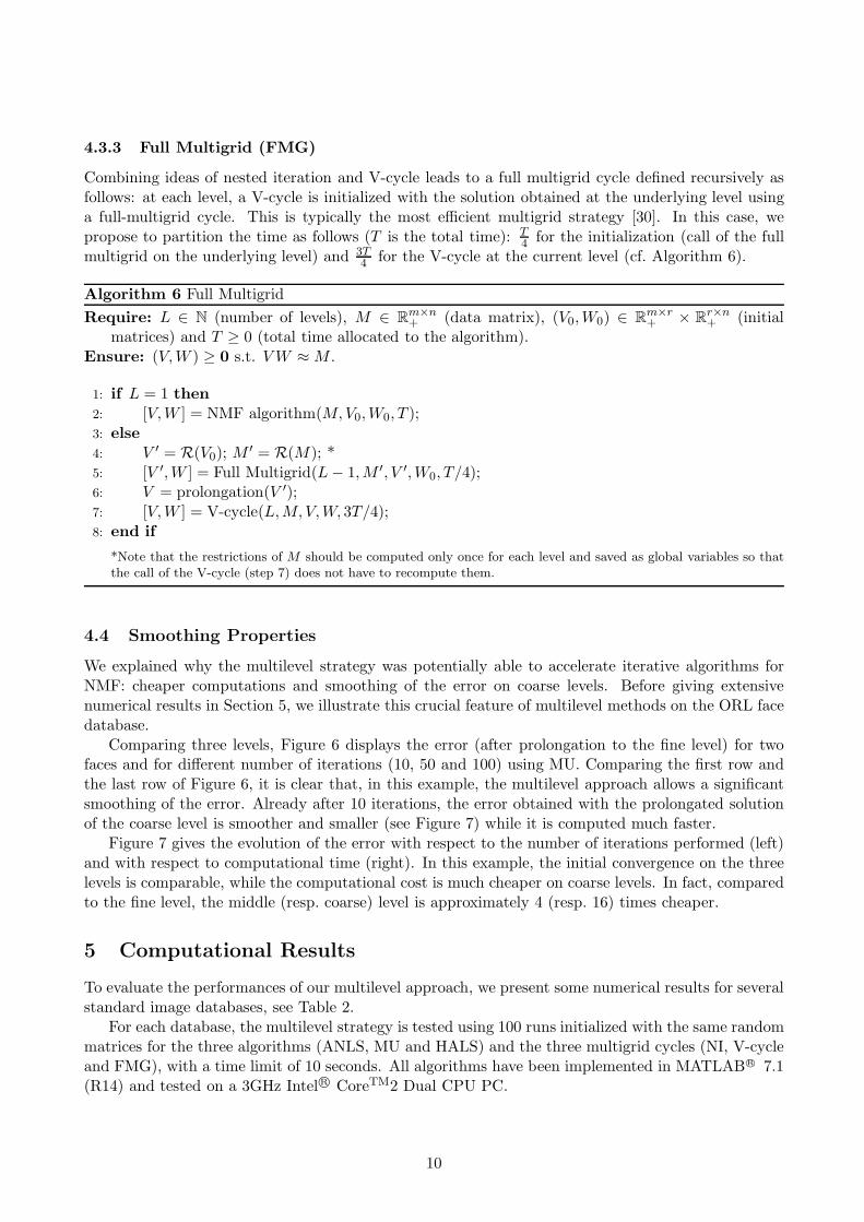
4.3.3 Full Multigrid (FMG)

Combining ideas of nested iteration and V-cycle leads to a full multigrid cycle defined recursively asfollows: at each level, a V-cycle is initialized with the solution obtained at the underlying level usinga full-multigrid cycle. This is typically the most efficient multigrid strategy [30]. In this case, wepropose to partition the time as follows (T is the total time): T

4 for the initialization (call of the fullmultigrid on the underlying level) and 3T

4 for the V-cycle at the current level (cf. Algorithm 6).

Algorithm 6 Full Multigrid

Require: L ∈ N (number of levels), M ∈ Rm×n+ (data matrix), (V0,W0) ∈ R

m×r+ × R

r×n+ (initial

matrices) and T ≥ 0 (total time allocated to the algorithm).Ensure: (V,W ) ≥ 0 s.t. V W ≈M .

1: if L = 1 then2: [V,W ] = NMF algorithm(M,V0,W0, T );3: else4: V ′ = R(V0); M ′ = R(M); *5: [V ′,W ] = Full Multigrid(L− 1,M ′, V ′,W0, T/4);6: V = prolongation(V ′);7: [V,W ] = V-cycle(L,M,V,W, 3T/4);8: end if

*Note that the restrictions of M should be computed only once for each level and saved as global variables so thatthe call of the V-cycle (step 7) does not have to recompute them.

4.4 Smoothing Properties

We explained why the multilevel strategy was potentially able to accelerate iterative algorithms forNMF: cheaper computations and smoothing of the error on coarse levels. Before giving extensivenumerical results in Section 5, we illustrate this crucial feature of multilevel methods on the ORL facedatabase.

Comparing three levels, Figure 6 displays the error (after prolongation to the fine level) for twofaces and for different number of iterations (10, 50 and 100) using MU. Comparing the first row andthe last row of Figure 6, it is clear that, in this example, the multilevel approach allows a significantsmoothing of the error. Already after 10 iterations, the error obtained with the prolongated solutionof the coarse level is smoother and smaller (see Figure 7) while it is computed much faster.

Figure 7 gives the evolution of the error with respect to the number of iterations performed (left)and with respect to computational time (right). In this example, the initial convergence on the threelevels is comparable, while the computational cost is much cheaper on coarse levels. In fact, comparedto the fine level, the middle (resp. coarse) level is approximately 4 (resp. 16) times cheaper.

5 Computational Results

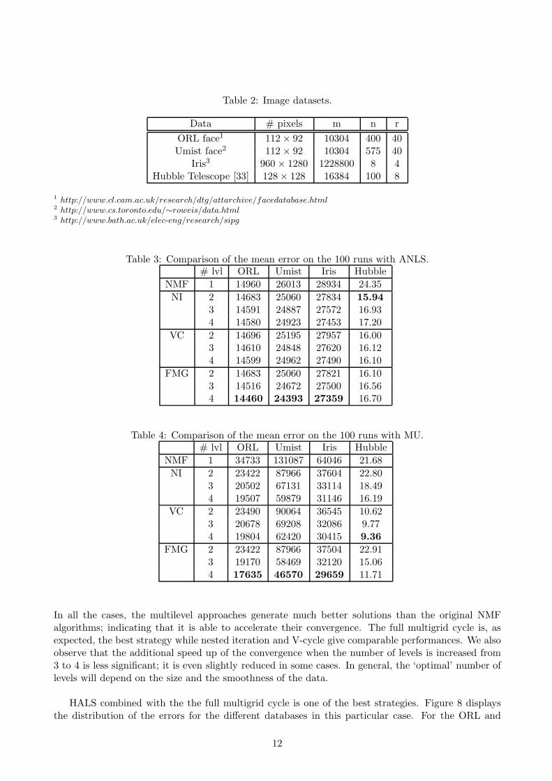
To evaluate the performances of our multilevel approach, we present some numerical results for severalstandard image databases, see Table 2.

For each database, the multilevel strategy is tested using 100 runs initialized with the same randommatrices for the three algorithms (ANLS, MU and HALS) and the three multigrid cycles (NI, V-cycleand FMG), with a time limit of 10 seconds. All algorithms have been implemented in MATLABR© 7.1(R14) and tested on a 3GHz IntelR© CoreTM2 Dual CPU PC.

10

Figure 6: Smoothing on Coarse Levels. Example of the smoothing properties of the multilevel approachon the ORL face database. Each image represents the absolute value of the approximation error (blacktones indicate a high error) of one of the two faces from the ORL face database. These approximationsare the prolongations (to the fine level) of the solutions obtained using the multiplicative updates ona single level, with r = 40 and the same initial matrices. From top to bottom: level 1 (fine), level 2(middle) and level 3 (coarse); from left to right: 10 iterations, 50 iterations and 100 iterations.

Figure 7: Evolution of the error on each level, after prolongation on the fine level, with respect to (left)the number of iterations performed and (right) the computational time. Same setting as in Figure 6.

5.1 Results

Tables 3, 4 and 5 give the mean error attained within 10 seconds using the different approaches.

11

Table 2: Image datasets.

Data # pixels m n r

ORL face1 112× 92 10304 400 40Umist face2 112× 92 10304 575 40

Iris3 960 × 1280 1228800 8 4Hubble Telescope [33] 128× 128 16384 100 8

1 http://www.cl.cam.ac.uk/research/dtg/attarchive/facedatabase.html2 http://www.cs.toronto.edu/∼roweis/data.html3 http://www.bath.ac.uk/elec-eng/research/sipg

Table 3: Comparison of the mean error on the 100 runs with ANLS.# lvl ORL Umist Iris Hubble

NMF 1 14960 26013 28934 24.35

NI 2 14683 25060 27834 15.943 14591 24887 27572 16.934 14580 24923 27453 17.20

VC 2 14696 25195 27957 16.003 14610 24848 27620 16.124 14599 24962 27490 16.10

FMG 2 14683 25060 27821 16.103 14516 24672 27500 16.564 14460 24393 27359 16.70

Table 4: Comparison of the mean error on the 100 runs with MU.# lvl ORL Umist Iris Hubble

NMF 1 34733 131087 64046 21.68

NI 2 23422 87966 37604 22.803 20502 67131 33114 18.494 19507 59879 31146 16.19

VC 2 23490 90064 36545 10.623 20678 69208 32086 9.774 19804 62420 30415 9.36

FMG 2 23422 87966 37504 22.913 19170 58469 32120 15.064 17635 46570 29659 11.71

In all the cases, the multilevel approaches generate much better solutions than the original NMFalgorithms; indicating that it is able to accelerate their convergence. The full multigrid cycle is, asexpected, the best strategy while nested iteration and V-cycle give comparable performances. We alsoobserve that the additional speed up of the convergence when the number of levels is increased from3 to 4 is less significant; it is even slightly reduced in some cases. In general, the ‘optimal’ number oflevels will depend on the size and the smoothness of the data.

HALS combined with the the full multigrid cycle is one of the best strategies. Figure 8 displaysthe distribution of the errors for the different databases in this particular case. For the ORL and

12

Table 5: Comparison of the mean error on the 100 runs with HALS.# lvl ORL Umist Iris Hubble

NMF 1 15096 27544 31571 17.97

NI 2 14517 25153 29032 17.373 14310 24427 28131 16.914 14280 24256 27744 16.92

VC 2 14523 25123 28732 17.373 14339 24459 28001 17.024 14327 24364 27670 17.04

FMG 2 14518 25153 29120 17.393 14204 23950 27933 16.694 14107 23533 27538 16.89

Figure 8: Distribution of the error among the 100 random initializations using the HALS algorithmwith a full multigrid cycle: (top left) ORL, (top right) Umist, (bottom left) Iris, and (bottom right)Hubble.

Umist databases, the multilevel strategy is extremely efficient: all the solutions generated with 2 and3 levels are better than the original NMF algorithm. For the Iris and Hubble databases, the difference

13

is not as clear. The reason is that the corresponding NMF problems are ‘easier’ because the rank ris smaller. Hence the algorithms converge faster to stationary points, and the distribution of the finalerrors is more concentrated.

In order to visualize the evolution of the error through the iterations, Figure 9 displays the evolu-tion of the objective function with respect to the number of iterations independently for each algorithmand each database using nested iteration as the multigrid cycle (which is the easiest to represent). Inall the cases, the prolongations of the solutions from the lower levels generate much better solutionsthat the one obtained on the fine level.

These test results are very encouraging: the multilevel approach for NMF seems very efficient andallows to speed up convergence of algorithms significantly.

6 Concluding Remarks

In this paper, a multilevel approach to speed up NMF algorithms has been proposed and its efficiencyhas been experimentally demonstrated. In order to use this technique, one needs to be able to designlinear operators preserving nonnegativity and transferring accurately the data between the differentlevels. To conclude, we give some directions for further research.

6.1 Extensions

We have only used our multilevel approach for a specific objective function (sum of squared errors) tospeed up three NMF algorithms (ANLS, MU and HALS) and to factorize 2D images. However, thiscan be easily generalized to any other objective function, any other iterative algorithm and appliedto other kind of smooth data. Moreover, other types of coarse grid definition, transfer operators andgrid cycle can be used and could potentially improve efficiency.

A limitation of the proposed approach is that the multigrid strategy is only applied to one di-mension of the matrix (because we did not assume that the different images are related to each otherin any way). However, in some applications, rows of matrix M might also be restricted to lowerdimensional spaces. For example, in hyperspectral data analysis, each column of matrix M representsan image at a given wavelength, while each row represents the spectral signature of a pixel [27]. Sincespectral signatures feature smooth components as well, the multilevel strategy can be used to reduceboth dimensions of the data matrix.

This idea can also be extended to Nonnegative Tensor Factorization (NTF) (see, e.g., [33] andreferences therein where it is used to analyze the hyperspectral Hubble telescope images) by usingmultilevel techniques for higher dimensional spaces.

6.2 Initialization

Several judicious initializations for NMF algorithms have been proposed in the literature and allowto speed up convergence and improve, in general, the final solution [12, 2]. The computational costof these good initial guesses depends on the matrix dimensions and will then be cheaper to computeon the coarsest grid. Therefore, it would be interesting to combine classical NMF initializationstechniques with our multilevel approach for further speed up.

6.3 Unstructured data

A priori, applying a multilevel method to data for which we do not have any information aboutthe matrix to factorize (and a fortiori about the solution) seems out of reach. In fact, in thesecircumstances, there is no sensible way to define the transfer operators.

14

Figure 9: Evolution of the objective function. From left to right : MU, ANLS and HALS. From topto bottom: ORL, Umist, Iris and Hubble databases. 1 level stands for the standard NMF algorithms.The initial points for the curves 2 levels and 3 levels are the prolongated solutions obtained on thecoarser levels using nested iteration, cf. Section 4.3. All algorithms were initialized with the samerandom matrices.

However, it is not hopeless to extend the multilevel idea to other type of data. For example, in textmining applications, the term-by-document matrix could be restricted by stacking synonyms or similartexts together (similarly as in [28]). Of course, this implies some a priori knowledge or preprocessingof the data (which should be cheap enough to be profitable).

15

References

[1] M. Berry, M. Browne, A. Langville, P. Pauca, and R. Plemmons, Algorithms and

Applications for Approximate Nonnegative Matrix Factorization, Computational Statistics andData Analysis, 52 (2007), pp. 155–173.

[2] C. Boutsidis and E. Gallopoulos, SVD based initialization: A head start for nonnegative

matrix factorization, Journal of Pattern Recognition, 41 (2008), pp. 1350–1362.

[3] J. H. Bramble, Multigrid methods, Number 294 Pitman Research Notes in Mathematic Series.Longman Scientific & Technical, UK, 1995.

[4] A. Brandt, Guide to multigrid development, W. Hackbusch and U. Trottenberg, eds., MultigridMethods, Lecture Notes in Mathematics, Springer, 960 (1982), pp. 220–312.

[5] W. L. Briggs, A Multigrid Tutorial, SIAM, Philadelphia, 1987.

[6] D. Chen and R. Plemmons, Nonnegativity Constraints in Numerical Analysis, in A. Bultheeland R. Cools (Eds.), Symposium on the Birth of Numerical Analysis, World Scientific Press.,2009.

[7] A. Cichocki, S. Amari, R. Zdunek, and A. Phan, Non-negative Matrix and Tensor Fac-

torizations: Applications to Exploratory Multi-way Data Analysis and Blind Source Separation,Wiley-Blackwell, 2009.

[8] C. Cichocki and A.-H. Phan, Fast local algorithms for large scale Nonnegative Matrix and

Tensor Factorizations, IEICE Transactions on Fundamentals of Electronics, Vol. E92-A No.3(2009), pp. 708–721.

[9] C. Cichocki, R. Zdunek, and S. Amari, Non-negative Matrix Factorization with Quasi-

Newton Optimization, in Lecture Notes in Artificial Intelligence, Springer, vol. 4029, 2006,pp. 870–879.

[10] , Hierarchical ALS Algorithms for Nonnegative Matrix and 3D Tensor Factorization, inLecture Notes in Computer Science, Vol. 4666, Springer, pp. 169-176, 2007.

[11] , Nonnegative Matrix and Tensor Factorization, IEEE Signal Processing Magazine, (2008),pp. 142–145.

[12] J. Curry, A. Dougherty, and S. Wild, Improving non-negative matrix factorizations through

structured initialization, Journal of Pattern Recognition, 37(11) (2004), pp. 2217–2232.

[13] M. E. Daube-Witherspoon and G. Muehllehner, An iterative image space reconstruction

algorithm suitable for volume ect, IEEE Trans. Med. Imaging, 5 (1986), pp. 61–66.

[14] I. Dhillon, D. Kim, and S. Sra, Fast Newton-type Methods for the Least Squares Nonnegative

Matrix Approximation problem, in Proc. of SIAM Conf. on Data Mining, 2007.

[15] N. Gillis and F. Glineur, Nonnegative Factorization and The Maximum Edge Biclique Prob-

lem. CORE Discussion paper 2008/64, 2008.

[16] , Nonnegative Matrix Factorization and Underapproximation. Communication at 9th Inter-national Symposium on Iterative Methods in Scientific Computing, Lille, France, 2008.

[17] S. Gratton, A. Sartenaer, and P. Toint, On Recursive Multiscale Trust-Region Algorithms

for Unconstrained Minimization, in Oberwolfach Reports: Optimization and Applications.

16

[18] J. Han, L. Han, M. Neumann, and U. Prasad, On the rate of convergence of the image space

reconstruction algorithm, Operators and Matrices, 3(1) (2009), pp. 41–58.

[19] N.-D. Ho, P. Van Dooren, and V. Blondel, Descent methods for nonnegative matrix factor-

ization, In: Numerical Linear Algebra in Signals, Systems and Control, Springer Verlag, (2008).

[20] H. Kim and H. Park, Non-negative Matrix Factorization Based on Alternating Non-negativity

Constrained Least Squares and Active Set Method, SIAM J. Matrix Anal. Appl., 30(2) (2008),pp. 713–730.

[21] C. Lawson and R. Hanson, Solving Least Squares Problems, Prentice-Hall, 1974.

[22] D. Lee and H. Seung, Learning the Parts of Objects by Nonnegative Matrix Factorization,Nature, 401 (1999), pp. 788–791.

[23] , Algorithms for Non-negative Matrix Factorization, In Advances in Neural Information Pro-cessing, 13 (2001).

[24] C.-J. Lin, On the Convergence of Multiplicative Update Algorithms for Nonnegative Matrix Fac-

torization, in IEEE Transactions on Neural Networks, 2007.

[25] , Projected Gradient Methods for Nonnegative Matrix Factorization, Neural Computation,19 (2007), pp. 2756–2779. MIT press.

[26] P. Paatero and U. Tapper, Positive matrix factorization: a non-negative factor model with

optimal utilization of error estimates of data values, Environmetrics, 5 (1994), pp. 111–126.

[27] P. Pauca, J. Piper, and R. Plemmons, Nonnegative matrix factorization for spectral data

analysis , Linear Algebra and its Applications, 406(1) (2006), pp. 29–47.

[28] S. Sakellaridi, H.-r. Fang, and Y. Saad, Graph-based Multilevel Dimensionality Reduction

with Applications to Eigenfaces and Latent Semantic Indexing. preprint, 2009.

[29] D. Terzopoulos, Image Analysis Using Multigrid Relaxation Methods, J. Math. Phys., PAMI-8(2) (1986), pp. 129–139.

[30] U. Trottenberg, C. Oosterlee, and A. Schuller, Multigrid, Elsevier Academic Press,London, 2001.

[31] M. Van Benthem and M. Keenan, Fast algorithm for the solution of large-scale non-negativity

constrained least squares problems, J. Chemometrics, 18 (2004), pp. 441–450.

[32] S. A. Vavasis, On the complexity of nonnegative matrix factorization, SIAM Journal on Opti-mization, 20 (2009), pp. 1364–1377.

[33] Q. Zhang, H. Wang, R. Plemmons, and P. Pauca, Tensor methods for hyperspectral data

analysis: a space object material identification study, J. Optical Soc. Amer. A, 25(12) (2008),pp. 3001–3012.

17

A Computational Cost of ANLS, MU and HALS

A.1 Active Set Methods for NNLS

In a nutshell, active set methods for nonnegative least squares work in the following iterative fash-ion [21]

1. get rid of the nonnegativity constraints and solve the unconstrained least squares problem cor-responding to the set of passive (nonzero) variables;

2. check the optimality conditions, if they are not satisfied:

3. update the sets of active (zero) and passive (nonzero) variables accordingly;

in such a way that that the objective function is decreased at each step.In (NMF), the problem of computing the optimal V (resp. W ) for a given fixed W (resp. V ) can

be decoupled into m (resp. n) independent NNLS subproblems in r variables:

minVi:∈R

r+

||Mi: − Vi:W ||2F , 1 ≤ i ≤ m (resp. min

W:j∈Rr+

||M:j − V W:j||2F , 1 ≤ j ≤ n).

Each of them amounts to solving a sequence of linear subsystems (with at most r variables, cf. step 1above) of

Vi:(WW T ) = Mi:WT , 1 ≤ i ≤ m (resp. (V T V )W:j = V T M:j, 1 ≤ j ≤ n).

In the worst case, one might have to solve every possible subsystem, which requires O(g(r)) operationswith4 g(r) =

∑ri=1

(ri

)

i3 = Θ(2rr3). Note that WW T and MW T (resp. V T V and V T M) can becomputed once for all to avoid redundant computations. Finally, one ANLS step requires at mostO(mnr + (m + n)s(r)r3) operations per iteration, where s(r) ≤ 2r. In the worst case, s(r) is inO(2r) while in practice it is in general much lower (as is the case for the simplex method for linearprogramming).

When m is reduced by a certain factor (e.g., 4 as in our experimental results), the computationalcost is not exactly reduced by the same factor because of the (m + n) factor above. However, in ourapplications, m (number of pixels) is much larger than n (number of images) and therefore one canapproximate the cost per iteration to be reduced by the same factor since m+n

4 ≈ m4 .

A.2 MU and HALS

The main computational cost of both MU and HALS resides in the computation of MW T , V T M ,WW T and V T V which requires 4mnr + 4(m + n)r2 = O(mnr) operations, cf. Algorithms 2 and 3.The computational cost is almost proportional to m (only the nr2 term is not, which negligible form≫ r).

4One can check that (2(r−3)− 1)(r − 2)3 ≤ g(r) ≤ 2rr3.

18

Recent titles CORE Discussion Papers

2010/6. Marc FLEURBAEY, Stéphane LUCHINI, Christophe MULLER and Erik SCHOKKAERT.

Equivalent income and the economic evaluation of health care. 2010/7. Elena IÑARRA, Conchi LARREA and Elena MOLIS. The stability of the roommate problem

revisited. 2010/8. Philippe CHEVALIER, Isabelle THOMAS and David GERAETS, Els GOETGHEBEUR,

Olivier JANSSENS, Dominique PEETERS and Frank PLASTRIA. Locating fire-stations: an integrated approach for Belgium.

2010/9. Jean-Charles LANGE and Pierre SEMAL. Design of a network of reusable logistic containers. 2010/10. Hiroshi UNO. Nested potentials and robust equilibria. 2010/11. Elena MOLIS and Róbert F. VESZTEG. Experimental results on the roommate problem. 2010/12. Koen DECANCQ. Copula-based orderings of multivariate dependence. 2010/13. Tom TRUYTS. Signaling and indirect taxation. 2010/14. Asel ISAKOVA. Currency substitution in the economies of Central Asia: How much does it

cost? 2010/15. Emanuele FORLANI. Irish firms' productivity and imported inputs. 2010/16. Thierry BRECHET, Carmen CAMACHO and Vladimir M. VELIOV. Model predictive control,

the economy, and the issue of global warming. 2010/17. Thierry BRECHET, Tsvetomir TSACHEV and Vladimir M. VELIOV. Markets for emission

permits with free endowment: a vintage capital analysis. 2010/18. Pierre M. PICARD and Patrice PIERETTI. Bank secrecy, illicit money and offshore financial

centers. 2010/19. Tanguy ISAAC. When frictions favour information revelation. 2010/20. Jeroen V.K. ROMBOUTS and Lars STENTOFT. Multivariate option pricing with time varying

volatility and correlations. 2010/21. Yassine LEFOUILI and Catherine ROUX. Leniency programs for multimarket firms: The

effect of Amnesty Plus on cartel formation. 2010/22. P. Jean-Jacques HERINGS, Ana MAULEON and Vincent VANNETELBOSCH. Coalition

formation among farsighted agents. 2010/23. Pierre PESTIEAU and Grégory PONTHIERE. Long term care insurance puzzle. 2010/24. Elena DEL REY and Miguel Angel LOPEZ-GARCIA. On welfare criteria and optimality in an

endogenous growth model. 2010/25. Sébastien LAURENT, Jeroen V.K. ROMBOUTS and Francesco VIOLANTE. On the

forecasting accuracy of multivariate GARCH models. 2010/26. Pierre DEHEZ. Cooperative provision of indivisible public goods. 2010/27. Olivier DURAND-LASSERVE, Axel PIERRU and Yves SMEERS. Uncertain long-run

emissions targets, CO2 price and global energy transition: a general equilibrium approach. 2010/28. Andreas EHRENMANN and Yves SMEERS. Stochastic equilibrium models for generation

capacity expansion. 2010/29. Olivier DEVOLDER, François GLINEUR and Yu. NESTEROV. Solving infinite-dimensional

optimization problems by polynomial approximation. 2010/30. Helmuth CREMER and Pierre PESTIEAU. The economics of wealth transfer tax. 2010/31. Thierry BRECHET and Sylvette LY. Technological greening, eco-efficiency, and no-regret

strategy. 2010/32. Axel GAUTIER and Dimitri PAOLINI. Universal service financing in competitive postal

markets: one size does not fit all. 2010/33. Daria ONORI. Competition and growth: reinterpreting their relationship. 2010/34. Olivier DEVOLDER, François GLINEUR and Yu. NESTEROV. Double smoothing technique

for infinite-dimensional optimization problems with applications to optimal control. 2010/35. Jean-Jacques DETHIER, Pierre PESTIEAU and Rabia ALI. The impact of a minimum pension

on old age poverty and its budgetary cost. Evidence from Latin America.

Recent titles CORE Discussion Papers - continued

2010/36. Stéphane ZUBER. Justifying social discounting: the rank-discounting utilitarian approach. 2010/37. Marc FLEURBAEY, Thibault GAJDOS and Stéphane ZUBER. Social rationality, separability,

and equity under uncertainty. 2010/38. Helmuth CREMER and Pierre PESTIEAU. Myopia, redistribution and pensions. 2010/39. Giacomo SBRANA and Andrea SILVESTRINI. Aggregation of exponential smoothing

processes with an application to portfolio risk evaluation. 2010/40. Jean-François CARPANTIER. Commodities inventory effect. 2010/41. Pierre PESTIEAU and Maria RACIONERO. Tagging with leisure needs. 2010/42. Knud J. MUNK. The optimal commodity tax system as a compromise between two objectives. 2010/43. Marie-Louise LEROUX and Gregory PONTHIERE. Utilitarianism and unequal longevities: A

remedy? 2010/44. Michel DENUIT, Louis EECKHOUDT, Ilia TSETLIN and Robert L. WINKLER. Multivariate

concave and convex stochastic dominance. 2010/45. Rüdiger STEPHAN. An extension of disjunctive programming and its impact for compact tree

formulations. 2010/46. Jorge MANZI, Ernesto SAN MARTIN and Sébastien VAN BELLEGEM. School system

evaluation by value-added analysis under endogeneity. 2010/47. Nicolas GILLIS and François GLINEUR. A multilevel approach for nonnegative matrix

factorization.

Books J. GABSZEWICZ (ed.) (2006), La différenciation des produits. Paris, La découverte. L. BAUWENS, W. POHLMEIER and D. VEREDAS (eds.) (2008), High frequency financial econometrics:

recent developments. Heidelberg, Physica-Verlag. P. VAN HENTENRYCKE and L. WOLSEY (eds.) (2007), Integration of AI and OR techniques in constraint

programming for combinatorial optimization problems. Berlin, Springer. P-P. COMBES, Th. MAYER and J-F. THISSE (eds.) (2008), Economic geography: the integration of

regions and nations. Princeton, Princeton University Press. J. HINDRIKS (ed.) (2008), Au-delà de Copernic: de la confusion au consensus ? Brussels, Academic and

Scientific Publishers. J-M. HURIOT and J-F. THISSE (eds) (2009), Economics of cities. Cambridge, Cambridge University Press. P. BELLEFLAMME and M. PEITZ (eds) (2010), Industrial organization: markets and strategies. Cambridge

University Press. M. JUNGER, Th. LIEBLING, D. NADDEF, G. NEMHAUSER, W. PULLEYBLANK, G. REINELT, G.

RINALDI and L. WOLSEY (eds) (2010), 50 years of integer programming, 1958-2008: from the early years to the state-of-the-art. Berlin Springer.

CORE Lecture Series

C. GOURIÉROUX and A. MONFORT (1995), Simulation Based Econometric Methods. A. RUBINSTEIN (1996), Lectures on Modeling Bounded Rationality. J. RENEGAR (1999), A Mathematical View of Interior-Point Methods in Convex Optimization. B.D. BERNHEIM and M.D. WHINSTON (1999), Anticompetitive Exclusion and Foreclosure Through

Vertical Agreements. D. BIENSTOCK (2001), Potential function methods for approximately solving linear programming

problems: theory and practice. R. AMIR (2002), Supermodularity and complementarity in economics. R. WEISMANTEL (2006), Lectures on mixed nonlinear programming.