Page 1
“Dead in the Short Run:
The Global Financial Crisis
and the Failure of Economic Policy”
by
Marcin Jerzy Michalski
BSc (Hons) Management specialising in International Business Economics
Student ID Number: 7657316
Supervised by Dr Terry Robinson
University of Manchester
Manchester Business School
2012/2013
Page 2
Declaration of Originality
This dissertation is my own original work and has not been submitted for any
assessment or award at University of Manchester or any other university.
Manchester, 3rd of May 2013
Marcin Jerzy Michalski
Page 3
3
Table of contents
Acknowledgements .................................................................................... 4
Abstract ...................................................................................................... 5
Preface ....................................................................................................... 6
The Crisis and the Recession ................................................................... 10
Pre-crisis Economic Policy ...................................................................... 26
Post-crisis Macroeconomic Environment ................................................ 37
The Unique Experience of Japan ............................................................. 51
Unconventional Monetary Policy ............................................................ 58
Quantitative Research .............................................................................. 65
Summary .................................................................................................. 85
Bibliography ............................................................................................ 88
Page 4
4
Acknowledgements
I would like to express my gratitude to all the people who provided me with their kind
help and thoughtful assistance during the long and challenging process of working on
this dissertation.
I would especially like to thank Dr Terry Robinson, my supervisor, for his expertise,
patience, and guidance that allowed me to stay on the right track from the start until
the very end of my work.
My gratitude is also extended to my parents and relatives, close friends, and my
academic advisor, Dr Paul Dewick, for their constant heartening and uplifting that
kept me motivated over the seven months I took to complete my work.
This dissertation would not have been possible without their extraordinary support
and encouragement.
Page 5
5
Abstract
More than six years after the beginning of the longest and the most painful period of
financial instability and economic turmoil since the Great Depression, economic
recovery still remains hesitant and uneven. This dissertation seeks to provide an
answer to two fundamental questions: “what caused the Global Financial Crisis?”, and
“are the policies adopted to foster economic recovery working?”.
The paper provides a theoretical discussion of the short-term and long-term causes of
the Financial Crisis, describes the post-crash macroeconomic environment and its
effects on the economic policies available to policy-makers, and provides
a comparative analysis of the Global Financial Crisis and the Japanese crisis of the
1990’s. It also presents the results of quantitative assessment of conventional
monetary policy, quantitative easing, and fiscal stimulation.
This dissertation identifies the originate-to-distribute lending model, leveraged
speculation on financial derivatives, the actions of the Government Sponsored
Entities, and the policy framework associated with the Great Moderation as the main
roots of the imbalanced economic environment, in which the Crisis could have
occurred. Furthermore, it recognises a number of similarities between the Global
Financial Crisis and the Japanese crisis of the 1990’s as far as both their causes and
the policy responses to them are concerned. Finally, it emphasises the need for fiscal
consolidation in advanced economies, while proving that quantitative easing has fairly
limited effects on recovery prospects.
Page 6
6
Preface
It has been more than six years since the beginning of the most painful and long-
lasting period of financial instability and economic downturn since the Great
Depression, and yet, despite tremendous efforts of the peoples and governments of the
countries most affected by the Global Financial Crisis, economic recovery still
remains very weak and fragile (Sullivan, 2009; Siegel, 2009). The Crisis and the
subsequent recession have been extremely costly thus far – it is impossible to provide
even an approximation of this cost, as apart from trillions of pounds lost due to the
decline of stock markets across the world, as well as due to the extensive bail-out and
stimulus programmes carried out in the most endangered economies, the turmoil in
the financial markets has cost millions of people their jobs, their homes, and their
future prospects (Financial Crisis Inquiry Commission, 2011). One thing, however, is
certain: this particular crisis and recession has already had an impact affecting not
only the current generation, but also the one that will follow.
Neither the financial markets, nor the policy makers were prepared for the possibility
that a crisis of such a magnitude and with such devastating effects could happen. The
sudden and unanticipated collapse of the global markets, and the sheer scale of the
crisis that it spurred, has also taken the vast majority of professional economists
aback. There were, however, voices of concern that predicted the collapse of the
housing market and a subsequent recession as early as in 2003, raised most notably by
Professors Robert J. Shiller and Karl E. Case, and by Dr Nouriel Roubini.
In their paper “Is There a Bubble in the Housing Market?” Case and Shiller (2003)
analysed the data on house prices in the biggest metropolitan areas in the United
States, and noticed that since 1995 they were rising much faster than incomes and
virtually all other prices. Their concluding remarks were rather worrying, stating that
property prices would probably stall at one point or even decline in some cities, which
would have tragic consequences for heavily indebted individuals, starting a wave of
personal bankruptcies. What happened between 2007 and 2009 exceeded their worst
expectations by far.
Page 7
7
Dr Roubini predicted the deflation of the housing bubble followed by a severe
recession in 2005, an issue he has discussed many times since. In 2006, he spoke at
the International Monetary Fund conference warning about the United States “facing
a once-in-a-life-time housing bust, an oil shock, sharply declining consumer
confidence and, ultimately, a deep recession” (Mihm, 2008). He anticipated an
increasing number of defaults on home mortgages, trillions of dollars of mortgage-
backed securities becoming worthless, and, finally, the global financial system
coming to a halt, which in effect would annihilate various hedge funds, investment
banks, and other financial institutions (Roubini, 2010). Although back in 2006 his
predictions were met with a healthy dose of scepticism, the harsh reality of the
financial crisis that began merely a year later has clearly matched his forecasts.
Unfortunately, only a very narrow group of economists, finance professionals, and
policy makers shared the seemingly unjustified apocalyptic view of the future of the
financial markets, and so the world was largely unprepared for the oncoming collapse
of the housing market and the devastating shockwaves it would send across the globe.
The issue described above, that is, whether the financial crisis could have been
avoided or at least predicted, was only one of the many themes of the academic and
political debate that followed immediately afterwards. Other important questions
raised in this debate range from that of what exactly caused the crisis and who is to
blame for it, through the steps that have to be taken in order to curb the recession and
foster economic growth, to the regulatory and policy changes that have to be adopted
in order to prevent a crisis of a similar nature from reoccurring. It is a confrontation
between various schools of economic thought, supporters of left-wing and right-wing
political policies, and even between the rich and the poor of the world. Bearing in
mind, however, that many economists and policy makers still disagree about the
causes of the Great Depression, and about the appropriate policy responses to it and
their effectiveness, even though it happened almost a century ago (see Friedman,
2002; Siegel, 2009; Stiglitz, 2010; Wapshott, 2011), this debate will surely carry on in
the foreseeable future.
The subject of this dissertation is of no small importance to the people and
governments of the developed Western nations. In 1923, in his “Tract on Monetary
Reform”, John Maynard Keynes famously stated that “in the long run we are all dead”
Page 8
8
(Keynes, 1924: p. 80). Although he was referring primarily to the fact that contrary to
the beliefs of classical economists, macroeconomics and its tools should principally
focus on short-term economic fluctuations, I believe that given the current very
difficult economic conditions that render many of the policy tools useless, it is fair to
paraphrase him by saying that right now we are dead in the short run. Providing an
explanation of how we arrived at this situation, together with answering at least some
of the questions mentioned above is the main aim of this dissertation.
With the Crisis still far from over, there is a clear need for further research into the
subject, as the more we know about it and the better we understand its nature, the
more effectively can it be tackled to promote further recovery and economic growth.
This dissertation has been written with the above statement in mind, and attempts to
provide answers to the following questions:
1. What were the immediate causes of the Global Financial Crisis?
2. How did the economic policy followed in the years leading up to the
meltdown of financial markets contribute to the escalation of the problem?
3. How did the post-crash economic environment influence the shape and design
of the policies implemented to counteract the Recession?
4. Are those policies effective? Have they had a significant impact on economic
recovery?
5. Was the Crisis truly unprecedented?
Put shortly, an analysis of the role that the economic policy followed by the Western
developed nations prior to 2007 played in the making and escalation of the Crisis,
together with the policy responses to it, and an assessment of their effectiveness
remains the ultimate objective of my work.
In order to set the stage for further discussion, the first chapter focuses on the Global
Financial Crisis itself, identifying its immediate causes and consequences, and
providing a brief overview of its evolution over time. The economic vulnerabilities
that sparked the crisis, however, were years in the making, as the policies adopted so
as to fuel and sustain the economic expansion almost indefinitely, primarily by
creating a virtually riskless society, simultaneously contributed to the formation of an
Page 9
9
asset bubble and the weakening of the soundness of the global financial system, which
is the subject of the second chapter.
The following chapter centres on the reaction of the policy makers to the crisis – in
2008 the world was forced to choose between two equally painful alternatives of
either allowing its financial system to collapse, or injecting trillions of pounds of
taxpayers’ money into the system to provide emergency funding to an increasing
group of companies. Some decisions were a necessary evil that provided short-term
stability but had undesirable long-term effects, turning one problem into another. For
example, the decision to bail out or nationalise the most endangered institutions might
have improved the short-term stability of the financial system, however, it has also
contributed to the rising levels of public debt in the United States, and in the United
Kingdom, forcing those countries to adopt severe austerity measures in order not to
default on their sovereign debt – a problem which thus far has cost them both their
highest AAA credit ratings.
The fourth chapter offers an insight into the Japanese housing bubble of the early
1990s and its “lost two decades” that followed. As George Santayana famously said,
“those who cannot remember the past are condemned to repeat it” (1905: p. 284). The
crisis and the economic stagnation that Japan has experienced are remarkably similar
to the Global Financial Crisis and the ongoing turmoil, both as far as their causes and
the policy responses are concerned. There are lessons to be learnt from the Japanese
experience of the last two decades, particularly regarding the subject of the
subsequent chapter, the unconventional monetary policy.
Finally, the sixth chapter outlines the methodology and the results of my empirical
work aimed at assessing the effectiveness of policies adopted post 2009 in order to
foster economic growth in the post-crisis period. It is followed by a brief review of the
discussion presented in this dissertation, which at this point can be summarised by a
quote from Reinhart and Rogoff’s book “This Time is Different”:
“Debt-fuelled booms all too often provide false affirmation of a government’s
policies, a financial institution’s ability to make profits, or a country’s standard of
living. Most of these booms end badly.” (Reinhart and Rogoff, 2009b: p. xxv).
Page 10
10
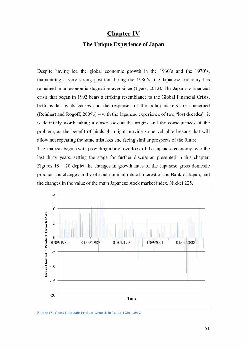
Chapter II The Crisis and the Recession
Figure 1: Major Indices Performance 2007 - 20121
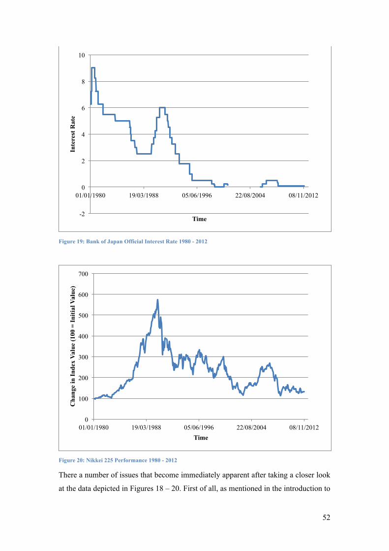
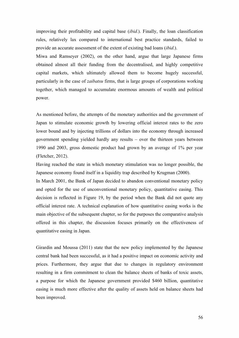
Figure 1 depicts the changes in the values of three market indices of a global
importance over the last five years – American Dow Jones Industrial Average, British
FTSE100, and Japanese Nikkei 225. The chart depicts the sheer scale of the losses
incurred as a direct result of the Global Financial Crisis – the aforementioned indices
lost between 50% and almost 70% in their values, as measured from the peak to the
trough, within only two years. Following the conclusion of the Second World War,
the Western world has experienced years of almost continuous rapid economic growth
– with the experience of the Great Depression almost forgotten, reflected primarily by
1 All charts depicting market data are the author’s own work based on data obtained through Bloomberg Database, unless indicated otherwise.
30
40
50
60
70
80
90
100
110
120
01/01/2007 15/05/2008 27/09/2009 09/02/2011 23/06/2012
Cha
nge
in In
dex
Valu
e (1
00 =
Initi
al V
alue
)
Time
FTSE100
Dow Jones
Nikkei 225
Page 11
11
the contents of history textbooks, a market decrease of this scale was absolutely
unprecedented and unanticipated.
The Global Financial Crisis is one of the rare cases when a financial crash triggers an
economic recession, rather than the other way around. Finance and economics,
however, are very closely related, almost intertwined, with one affecting the other,
and therefore an investigation of the economic policy followed in the years leading up
to a crisis frequently sheds some light on the causes of a financial crash. This issue is
analysed in this and the following chapter of this dissertation, with the former
focusing on the more immediate causes of the crisis, and the latter on the economic
factors that created an imbalanced environment in which it could have occurred.
Although the main focus of this chapter is placed on the American mortgage and
stock market, primarily because it was where the Global Financial Crisis originated,
the issues discussed below were much more widespread and took place in almost all
countries affected by the Crisis.
One of the most important factors affecting the behavioural patterns of market
participants is their attitude towards risk, which means that their actions will be
defined largely by their perception of the current systemic risk in the market. Before
the discussion presented in this chapter moves on to the analysis of the causes of the
Global Financial Crisis, it is worth looking into the attitude that dominated the
financial markets in the years leading up to their meltdown.
This of course leads to one important question: is it possible to express someone’s
attitude towards risk in a quantitative manner? After all, as any other personal
preference, it varies with every individual. In the early 1990s, however, using the data
on S&P100 Index option prices, R.E. Whaley developed the Chicago Board Options
Exchange Market Volatility Index, known as the VIX Index, or the investor fear
gauge.
As explained by Whaley (2009), the VIX is a forward looking measure of expected
stock market volatility over the next 30 days implied by the current price of options
on S&P500 Index. Although volatility is a measure of unexpected upward or
downward market movements, S&P500 index put options are commonly used by
hedgers, particularly when they believe that the value of their portfolio will decrease
in the future (Whaley, 2009). An increase in demand for put options increases their
Page 12
12
price and implied volatility, and hence it is reasonable to conclude that the higher
expected stock market volatility implicated by option prices corresponds to higher
levels of fear among investors.
Figure 2 depicts the values of the VIX Index between January 1990 and December
2012. Generally speaking, before the Global Financial Crisis occurred the index value
spiked to a level of about 40 – 45% a number of times, only to return to its ‘natural’
level of 15 – 25% (portrayed as blue area in Figure 2) shortly afterwards. The two
substantial increases in value that occurred in 1997 and 1998 were a result of
a substantial sell-off of stocks and the period of unrest that followed. The next peak
occurred in September 2001 and can be associated with the time of widespread
anxiety that followed the September 11 terrorist attacks. The increase in the value of
the index in that period can also be associated with the deflation of the Internet stocks
bubble, and the unravelling of various corporate governance scandals. After 2003,
however, the level of the index returned to the region of 10 – 15%, where it remained
until early 2007.
The beginning of 2007 marked the first defaults of homeowners’ on their mortgages.
What is interesting, however, is the fact that after the period of initial unrest, the index
decreased to about 18%, only to rocket to the value of more than 80% in September
2008 following the bankruptcy of Lehman Brothers. It took almost two years for the
index to temporarily return to the value of below 20%.
Figure 2: Investor Fear Index 1990 - 2012
0
10
20
30
40
50
60
70
80
90
01/01/1990 09/02/1994 20/03/1998 28/04/2002 06/06/2006 15/07/2010
Inde
x Va
lue
Time
Page 13
13
The interpretation of this data is fairly straightforward – it depicts a period of
prolonged euphoria and overconfidence of market participants (green area in Figure
2) fuelled by the actions of the Federal Reserve aimed at counteracting the negative
effects of the deflation of the dot.com bubble, explained in detail in the next chapter.
It was, however, a period of calm before a storm, as the behaviour of the index
between 2008 and late 2011 is typical of a widespread panic in the market (red area in
Figure 2).
In its report, the Financial Crisis Inquiry Commission (2011) concludes that the Crisis
occurred due to a number of factors, most notably:
− Declining mortgage-lending standards and mortgage securitisation;
− Failure to provide adequate credit worthiness assessment by credit rating
agencies;
− The impact of over-the-counter derivatives, particularly Mortgage Backed
Securities (MBS), Collateralised Debt Obligations (CDO), and Credit Default
Swaps (CDS);
− Destabilisation of financial markets due to failures in regulation and
supervision;
− Systematic lack of adequate corporate governance and risk management in
financial institutions;
− Combination of excessive borrowing, risky investments, and lack of financial
transparency;
− Inconsistent response of the governments, which fuelled the uncertainty and
panic in the financial markets.
A detailed discussion of all of the aforementioned issues would go far beyond the
objectives and the scope of this dissertation, therefore the analysis presented in this
chapter will focus only on the most important aspects, offering some basic insights
sufficient to gain a good understanding of the underlying problem.
Four of the factors identified above, that is declining lending standards, excessive
borrowing, mortgage securitisation, and the impact of financial derivatives, will be
discussed together, particularly as they represent elements of a cause and effect chain
that shook the foundations and the soundness of the financial system.
Page 14
14
Siegel (2009) points out that the decline in market values and the losses on
a mammoth scale incurred by the once-proud financial institutions, interconnected
through a series of complex financial instruments to the extent that the whole global
financial system was at the point of collapse, had a very unlikely cause – leveraged
speculation on home mortgages.
As explained by Buckley (2011), two decades ago, the lending models used by
various banks were based on the originate-to-hold principle, involving issuing
a mortgage against the security of a home with the bank receiving regular interest and
capital repayments until its maturity. Under this model the bank would hold the
mortgage for a very long time, and hence would be very careful about its customers’
ability to repay it by conducting all the necessary credit assessments and due diligence
procedures. In the late 1990s, however, this model has been replaced by the originate-
to-distribute model, in which the mortgage is no longer held by a bank but instead is
sold on to another institution, where a series of similar loans are repackaged and sold
further on as a mortgage backed security. The institution which purchased the
mortgage might also mix it up with a series of other loans, such as credit card debt,
student loan, and corporate loan, and then sell the package as a collateralised debt
obligation.
A mortgage backed security is a particular type of an asset backed secuity, that is an
instrument created from a portfolio of income-producing assets, which is then sold to
a special purpose vehicle, usually operated by an investment bank or a Government
Sponsored Entity allocating the cashflows generated by interest payments and capital
repayments to groups of investors, known as tranches (Hull, 2012). A collateralised
debt obligation works on a similar principle, however, as pointed out in the previous
paragraph, its portfolio of underlying assets includes different types of debt
obligations. The creators of MBSs and CDOs assumed that defaults on home
mortgages occur randomly and only a few homeowners default in any given time, so
a combination of a series of mortgages allows to separate the safe part of mortgages
from the risky one without knowing which mortgages would default in the future,
ultimately creating a safe tradable security (Temin, 2010). Figure 3 illustrates how
MBSs and CDOs work using an example of a portfolio of debt obligations worth £500
million, with an average yield of 10% of interest per year equivalent to £50 million
per annum.
Page 15
15
As explained by Kilbeam (2010), a typical asset backed security would represent
a pool of loans of different quality, including prime mortgages (highest quality of
borrower), Alt-A mortgages (risk profile between prime and subprime), and subprime
mortgages (issued to clients with the lowest credit rating). The originator of the
mortgage would attempt to offset the substantial risk associated with holding loans of
poor quality on its balance sheet by selling them to be repackaged as either a MBS or
a CDO. The newly created derivative would be divided into tranches corresponding to
the riskiness of the underlying assets included in the portfolio of debt obligations.
Figure 3: A simplified MBS/CDO2
The original pool of obligations has a principal of £500 millions divided between the
four tranches, with each tranche promised a return on its investment corresponding to
its credit rating (the better the rating, the lower the promised returns). Once interest
and principal payments on original debt obligations are made, the cashflows generated
in the process are distributed by the special purpose vehicle to the participating
investors in a process known as the waterfall – the senior tranche is the first one to
have its claims settled, then the payment is made to the mezzanine tranche from the
funds left over after the first payment, and the process continues until either all claims
have been settled or the whole cashflow has been distributed (Hull, 2012).
2 Pilbeam, K. (2010), p.414
Mortgage backed security or collateralised debt obligation
Special purpose vehicle
Original mortgages and
debt obligations
Package of £500m of debt
obligations, average yield
10% of interest p.a. (£50m)
SPV (Distribution of
cashflows)
5% Tranche 1 (£25m) 30% p.a. (£7.5m)
Equity tranche (Not rated)
20% Tranche 2 (£100m) 15% p.a. (£15m)
Junior tranche (BBB rating)
25% Tranche 3 (£125m) 10% p.a. (£12.5m)
Mezzanine tranche (A rating)
50% Tranche 4 (£250m) 6% p.a. (£15m)
Senior tranche (AAA rating)
Page 16
16
Hull (2012) points out, however, that even though the equity tranche promises the
highest annual returns, it is the most likely to suffer the losses on its investment. The
value of the cashflows distributed between the tranches depends on the value of the
underlying assets. Hence, any fall in their value will correspond to a loss of the equity
tranche, whereas a fall exceeding 5% (£25m in the example) will mean that the equity
tranche investors will not get any money at all. The same principle applies to other
tranches, for example a 10% (£50m) decrease in value of the underlying assets will
result in some loss incurred by the junior tranche, but a fall of 20% (£100m) or more
will mean that their claims will not be settled at all.
This possibility meant that while finding investors willing to purchase AAA-rated
senior tranches was not too difficult, finding clients interested in the lower hierarchy
tranches was more problematic. In order to overcome this issue, markets introduced
variations of collateralised debt obligations, such as CDO2, which is a derivative
instrument based upon a package of existing CDOs or tranches of differing CDOs
(Pilbeam, 2010). This procedure allowed splitting a BBB-rated junior tranche into
a number of other tranches with ratings ranging from AAA to no rating at all.
The fact that a newly originated mortgage would not be kept on the balance sheet of
a lending institution, as it was sold on for the purposes of securitisation as soon as
possible, meant that under the originate-to-distribute lending model, the assessment of
the borrowers’ creditworthiness would not be of a great importance to the originator
(Buckley, 2011). Pilbeam (2010) argues that since a mortgage broker was paid an
upfront fee for each arranged mortgage, with no possibility of a penalty if the
mortgagee went into default later on, the originate-to-distribute model emphasised
quantity over quality. Furthermore, he points out that since the vast majority of the
subprime mortgages were adjustable rate mortgages, that is mortgages offering low
initial interest rates which would increase significantly after one or two years, they
attracted a larger proportion of borrowers who would be more likely to default on
payments than what was typically expected for Alt-A or prime mortgagees.
Buckley (2011) mentions that even though the traditional mortgage lending criteria
had been on the basis of the lower of three times the borrower’s income or 90 to 95%
of the value of the property mortgaged, in the run up to the crisis Northern Rock, via
its ‘Together’ brand, was offering a deal of 125% based on 95% of the property value
Page 17
17
with additional 30% in an unsecured loan and a lending facility based on six times the
income.
Credit default swaps were another very important financial derivative instruments that
played a major role in the escalation of the Global Financial Crisis. A CDS is
a contract that provides insurance against the risk of a default or other credit event by
a particular reference entity – the buyer of the insurance obtains the right to sell
corporate bonds issued by the reference entity for their face value when a credit event
occurs, in exchange for making periodic payments to the seller of the contract until it
expires or until a credit event happens (Hull, 2012). Figure 4 provides a graphical
representation of a credit default swap.
Figure 4: Credit default swap3
Although compared to any asset-backed security it is a much less complex derivative
product, a credit default swap has certain features that make it at least equally
interesting.
First of all, as explained by Buckley (2011), a CDS is primarily used to hedge the risk
that the reference company will fail to provide capital repayments to the protection
buyer, however, it can also be used for speculation purposes – neither of the parties to
the contract is required to actually own the underlying asset issued by the reference
entity, nor does it have to suffer a loss due to an occurrence of a credit event in order
to be eligible to receive the insured amount.
Secondly, unlike in typical insurance contracts, there is no legal limit to the number of
CDSs that can be entered into in reference to a particular company – it is therefore
possible that despite the reference entity having only £1 million of debt the
outstanding CDS contracts on that debt could amount to £100 million or even more.
3 Hull, J.C. (2012), p. 549
Page 18
18
Finally, credit default swaps could be written on virtually any type of asset that
displayed any probability of a default – ranging from corporate or government issued
bonds to mortgage backed securities and collateralised debt obligations.
Similarly to the mortgage backed securities and collateralised debt obligations, the
issuers of credit default swaps assumed that defaults occur randomly and irregularly,
and therefore the fixed periodic payments should exceed the expected value of the
pay-out should a credit event ever occur. Unfortunately, as pointed out by Buckley
(2011), what was assumed to be the worst-case scenario happened in real life, and so
when a wave of en masse defaults on mortgages and other debt obligations finally
took place, what used to be an asset on a financial institution’s balance sheet suddenly
became a liability.
The popularity of the three types of derivative instruments described above had
profound effects for the whole financial system, particularly when the sheer sizes of
their markets have been taken into account. The subprime mortgage market had debt
outstanding of $1.3 trillion at its peak, whereas at its highest point the credit default
swaps market had $60 trillion outstanding. It can therefore be easily argued that it was
the credit default swaps market that served as a catalyst turning a painful but
containable crash of subprime mortgages market into a crisis that threatened the
existence of the whole global financial system (Buckley, 2011).
The analysis presented thus far in this chapter, identifying the various derivative
products as the main drivers of excessive credit growth, is, however, only one side of
the coin. In his paper, Wallison (2009) presents an alternative view in which he
considers the role played primarily by the government and the two American
Government Sponsored Entities, Fannie Mae and Freddie Mac.
Wallison (2009) points out the fact that since the beginning of the 20th century, the
United States government had a policy of promoting homeownership by regularly
introducing new laws aimed at increasing the volume of mortgages made by banks.
Traditionally, when assessing an application for a mortgage, a lending institution
would take into account the overall financial position of the applicant, offering lower
interest rates for the borrowers of the highest standing, and demanding higher interest
payments from those in a more precarious financial position (Cooper, 2010). Once the
financial position of an individual becomes so weak that a bank arrives at the
Page 19
19
conclusion that there is no viable rate of interest at which a loan could be originated
without pushing the borrower further into insolvency, the applicant finds himself in
what is known as the poverty trap. In order to address this discrepancy between
government policy and private lending policies, in 1977 the United States government
adopted the Community Reinvestment Act giving it the powers to deny a bank’s
application for expansion if the applicant had failed to lend sufficiently in minority
neighbourhoods. Through adaptation of the Community Reinvestment Act the
government was effectively forcing commercial banks to take the risks they had
previously steered clear of. In effect, the banks were required to suspend their typical
prudent lending practices in order to make mortgages more affordable for borrowers
who were previously unable to meet the standards in the prime mortgage market.
Wallison (2009) argues, however, that the loans initially originated because of the
Community Reinvestment Act were not of weak enough quality to produce a financial
crisis, although they had triggered off a process of gradual spreading of low quality
loans to the rest of the mortgage market – by 2006 almost half of all mortgages
originated in the United States were either subprime or Alt-A mortgages.
Fannie Mae and Freddie Mac are two Government Sponsored Entities (GSEs)
operating in the United States set up with the purpose of counteracting the issues
associated with a poverty trap by providing a consistent supply of mortgage funds. In
order to achieve this objective the GSEs would purchase the loans from their
originators, and then securitise them while providing a guarantee of timely interest
and capital repayments, ultimately selling the newly created mortgage backed security
to other investors. This business mechanism established and maintained a constant
flow of funds between investors and lending institutions, allowing the latter to issue
more loans with lower interest rates due to a guaranteed inflow of funds from the
GSEs.
Simkovic (2013) argues that until mortgage backed securities were allowed to be
issued by investment banks, the securities created by Government Sponsored Entities
were of the highest standard due to the very scrupulous procedures of selecting the
affiliated lending institutions, which gave them a degree of control and surveillance
over the mortgage market. Wallison (2009), however, presents a point of view
contrasting to the one described above, placing the blame for the exuberance of the
subprime mortgage market on Fannie Mae and Freddie Mac.
Page 20
20
The original objective of these two GSEs was to maintain a liquid secondary market
for mortgages, however, by 1992 it was expanded to include promotion of affordable
housing. This had profound effects for the whole market, as due to their nature GSEs
were able to gain access to virtually unlimited amounts of capital at a very low cost,
and because of the specifics of their statutory regulations they were also allowed to
maintain a gearing ratio of 60:1 – these advantages allowed them to dominate the
market. Wallison (2009) points out that by 2005 the regulations of the Department of
Housing and Urban Development required the purchases of Fannie Mae and Freddie
Mac to consist of 55% of loans given to low- and moderate income borrowers, and
another 25% of loans given to low- or very-low income borrowers, which means that
the real work of reducing the quality of lending was done by the GSEs operating to
meet the government’s affordable housing regulations.
The funding advantages of Government Sponsored Entities allowed them to dominate
investment banks in the housing financing market – until the early 2000s, when
Fannie Mae and Freddie Mac began purchasing subprime mortgages in substantial
amounts, investment banks were interested only in either jumbo mortgages, which
exceeded the size of a loan that the law allowed GSEs to buy, or in junk mortgages
(Wallison, 2009). Until 2004 GSEs used to purchase large amounts of AAA-rated
tranches of asset backed securities from investment banks, but following a substantial
refinancing process that took place in 2003, however, they began buying subprime
and Alt-A mortgages directly from their originators in order to avoid paying
intermediation fees to investment banks – when a government-backed institution with
unlimited funds requests a delivery of low quality loans, it is only natural that the
market for them is going to rapidly expand.
The argument presented in Wallison’s paper (2009) can be summarised by saying that
Government Sponsored Entities were indirectly responsible for turning a painful
housing bubble deflation into a worldwide financial crisis, as they drove the
expansion of subprime mortgage market and the inflation of housing prices, which
leads to a conclusion that perhaps contrary to the opinion preserving in the media and
certain groups within the society, the Global Financial Crisis was not a crisis of
capitalism but a crisis of government.
Page 21
21
Another issue worth looking into is the degree to which financial institutions
increased their gearing in the run up to the crisis. Gearing is one of the commonly
used techniques that allows a company to increase its profitability by changing the
composition of its balance sheet, most importantly, the proportion of assets to equity.
Pilbeam (2010) points out that there is one substantial problem with gearing – even
though it increases returns and profits in good times, it also increases the risk levels
and therefore the dangers faced by a firm in periods of negative returns. In 2007,
Lehman Brothers reported a gearing ratio of 30.7:1 – this value of gearing means that
a mere 3% decline in the value of the assets held by the firm would result in losses
that have the potential to drive the company into bankruptcy.
Figure 5 illustrates the values of gearing ratios of five major investment banks
reported in their annual 10-K forms submitted to the Securities and Exchange
Commission. Bearing in mind that finance researchers estimate the value of an
optimal gearing ratio for a large investment bank to be between 10:1 and 15:1, the
figures presented below show that the excessive borrowing expansion did not take
place only in the personal lending market.
Figure 5: Gearing levels of major investment banks4
4 Based on annual 10-K forms submitted by the analysed companies to the Securities and Exchange Commission between 2003 - 2007
0
5
10
15
20
25
30
35
2003 2004 2005 2006 2007
Gea
ring
rat
io
Time
Goldman Sachs
Merill Lynch
Lehman Brothers
Morgan Stanley
Bear Stearns
Page 22
22
As indicated before, a full analysis of all the issues contributing to creation of the
extreme fragility of the financial markets goes far beyond the scope of this
dissertation and would not facilitate the analysis of its main topic. For this reason,
a range of other important issues of a more legal nature have not been investigated or
mentioned – chief among them, the question of the deregulation of financial markets,
introduced as part of the Reagan-Thatcher economic model, the one of the
consequences of the repeal of Glass-Steagall act, both, as proved by Wallison (2009),
with an impact significantly exaggerated by the media (the market for credit default
swaps was never formally regulated, so the claims of its “deregulation” are not
supported by any legal evidence), and the one of corporate governance of high-profile
financial institutions. A careful explanation of the originate-to-distribute model of
lending and the impact of complex derivative instruments, as well as other factors
driving the growth of subprime mortgage markets, should however be sufficient to
provide a basic picture of the growing interconnectedness and fragility of financial
markets prior to their crash.
In 2003, Professors Robert J. Shiller and Karl E. Case predicted that the rapid growth
in property prices would have come to a stall in the foreseeable future, and with the
housing market peaking in the United States in the middle of 2006, it is fair to say
they were absolutely correct. Figure 6 depicts the changes in the average value of
properties in the twenty biggest metropolitan areas of the United States measured by
the Case-Shiller index, and contrasts it with the performance of the S&P500 index.
Figure 6: Changes in stock market and housing market values
0
50
100
150
200
31/01/2000 27/10/2002 23/07/2005 18/04/2008 13/01/2011
Cha
nge
in v
alue
(100
= in
itial
val
ue)
Time
Housing Market
S&P 500
Page 23
23
One rather obvious conclusion that can be drawn from the chart above is that an
investment in property would significantly outperform one in the stock market – the
value of an average property more than doubled between 2000 and 2006, when at the
same time the stock market struggled to regain the value it reached in early 2000s. All
market booms, however, end one day, and the housing-market boom was no different.
With the value of the underlying assets declining since 2006, the required repayments
of mortgages taken to finance the acquisitions of property were increasing beyond the
financial capabilities of many borrowers, particularly the NINJAs (No verified
Income, Job or Assets) mortgagees. Unsurprisingly then, the beginning of 2007 was
marked by a growing number of delinquencies and defaults on subprime and Alt-A
mortgages.
By the first week of March 2007, many financial institutions realised that the
portfolios of asset-backed securities they were holding on their balance sheets
displayed higher delinquencies rates than the ones built into the models used for
pricing them (Buckley, 2011). The apparently almost risk-free securities purchased en
masse by Government Sponsored Entities, investment banks, and other corporations
have suddenly become toxic assets rapidly losing their value.
Between April and August 2007, many of the biggest American subprime lending
institutions went bankrupt, or narrowly escaped bankruptcy by taking emergency
loans worth billions of dollars from other banking firms. The situation in Europe was
not any better, as many mortgage companies began to fail as well, or had to be
rescued by the government – following a first bank run that happened in Britain in
decades since 1866, on the 17th of September 2007 the Chancellor of the Exchequer
had to approve government’s guarantee for Northern Rock’s existing deposits. Few
weeks later the central banks in the United States, the United Kingdom, the Eurozone,
and other economies were forced to announce injections of funds aimed at
counteracting freezing up of the short-term lending markets (Buckley, 2011).
As mentioned before, one particular disadvantage of high levels of gearing is that it
exposes the firm to increased dangers in the periods of negative returns. Taking into
account that many investment banks had used the additional capital raised through
gearing to invest in a portfolio of mortgage backed securities, collateralised debt
obligations, and credit default swaps, their situation became quite desperate as the
Page 24
24
value of the assets held on their balance sheets almost disappeared in a matter of
months. One famous example is the forced acquisition of Bear Stearns, a corporation
sold to J.P. Morgan Chase for $240 million, an equivalent of less than 1% of what it
was worth less than a month before. The Federal Reserve was another party to the
settlement, agreeing to underwrite $30 billion of Bear Stearns toxic assets (Pilbeam,
2010).
The situation of other banks was equally hopeless – on the 1st of April 2008 UBS
announced a $10 billion write off, less than three weeks later Citigroup wrote down
$15.2 billion of assets, and on the 16th of June Lehman Brothers announced a net loss
of $2.8 billion for the second quarter alone.
By 2008 Fannie Mae and Freddie Mac had $5.5 trillion worth of asset backed
securities on their balance sheet – both GSEs suffered losses on such a scale that the
U.S. government had to step in on the 7th of September and take the two firms into
conservatorship.
A week later another investment bank, Merrill Lynch, was taken over by the Bank of
America, and the following day, on the 15th of September, Lehman Brothers filed for
bankruptcy. The situation became even more difficult when the American
International Group, the largest counterparty in the credit default swaps market, with
obligations to only its five biggest institutional clients worth almost $30 billion, had to
accept emergency financial aid from the government amounting to $85 billion in
exchange for 79.9% ownership stake on the 16th of September, just a day after the fall
of Lehman Brothers (Buckley, 2011).
The examples mentioned above were only the tip of the iceberg, as practically every
single important financial institution in the world witnessed the value of its ‘safe’
assets decreasing so rapidly that raising the necessary capital to offset their losses was
close to impossible. One of the Federal Reserve’s stress tests carried out on the
sample of the largest investment banks in the United States estimated that the losses
they would incur between 2009 and 2010 would amount to more than $600 billion,
with further $185 billion required to maintain their minimum capital ratios (Federal
Reserve, 2009).
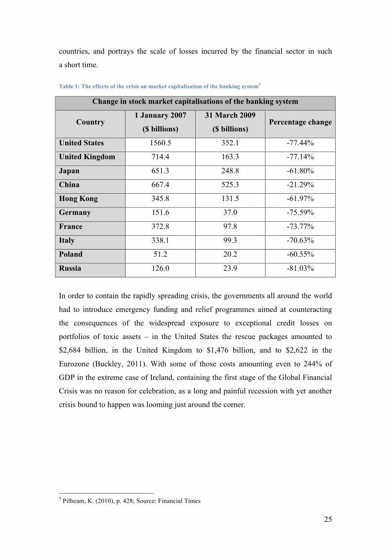
Table 1 presents the percentage change between the 1st of January 2007 and the 31st of
March 2009 of the stock market capitalisations of the banking systems in various
Page 25
25
countries, and portrays the scale of losses incurred by the financial sector in such
a short time.
Table 1: The effects of the crisis on market capitalisation of the banking system5
Change in stock market capitalisations of the banking system
Country 1 January 2007
($ billions)
31 March 2009
($ billions) Percentage change
United States 1560.5 352.1 -77.44%
United Kingdom 714.4 163.3 -77.14%
Japan 651.3 248.8 -61.80%
China 667.4 525.3 -21.29%
Hong Kong 345.8 131.5 -61.97%
Germany 151.6 37.0 -75.59%
France 372.8 97.8 -73.77%
Italy 338.1 99.3 -70.63%
Poland 51.2 20.2 -60.55%
Russia 126.0 23.9 -81.03%
In order to contain the rapidly spreading crisis, the governments all around the world
had to introduce emergency funding and relief programmes aimed at counteracting
the consequences of the widespread exposure to exceptional credit losses on
portfolios of toxic assets – in the United States the rescue packages amounted to
$2,684 billion, in the United Kingdom to $1,476 billion, and to $2,622 in the
Eurozone (Buckley, 2011). With some of those costs amounting even to 244% of
GDP in the extreme case of Ireland, containing the first stage of the Global Financial
Crisis was no reason for celebration, as a long and painful recession with yet another
crisis bound to happen was looming just around the corner.
5 Pilbeam, K. (2010), p. 428; Source: Financial Times
Page 26
26
Chapter II Pre-crisis Economic Policy
The previous Chapter focused primarily on the immediate causes of the Global
Financial Crisis and the recession that followed, identifying the originate-to-distribute
lending model and the actions of the Government Sponsored Entities as the main
drivers fuelling the excessive lending in the United States, and the wide-spread
leveraged speculation on asset-backed securities as the main issue leading to the
collapse of the financial markets in mid-2007. The analysis presented in this chapter
investigates the economic policy followed in the years leading up to the Crisis, in
order to establish the extent of the role it played in creating the imbalanced economic
environment in which a disaster of such a magnitude could have occurred.
In their paper, Barnett and Chauvet (2008) presented an argument that the Global
Financial Crisis brought an end to the Great Moderation – an episode in the history of
the economic development of the Western world characterised primarily by a very
low volatility of the business cycle, frequently viewed as a direct result of
developments and improvements in monetary policy.
The magnitude of the decline in the volatility of the business cycle was very
significant, as it decreased by a factor of three over the period of the Great
Moderation, due to smarter countercyclical economic policy, and to lower output and
inflation volatility that occurred around the same time, both associated with better
monetary policy (Blanchard and Simon, 2001). Another possible explanation for this
sharp decrease in volatility was presented by McConnell and Perez-Quiros (2000),
who argued that it was driven primarily by a reduction of volatility in the durables
production, which also corresponds to a drop in durables output in favour of inventory
investment, possibly suggesting a shift from goods production to services.
Figures 7 and 8 provide an overview of the post-Second World War real gross
domestic product growth rates in the United States, and in the United Kingdom
respectively, with the period of the Great Moderation reflected by the shaded areas of
the two charts. Indeed, as suggested above, some time around the early 1980s, the
Page 27
27
pattern of the behaviour of the data changed significantly, as the amplitude of the
business cycle fell dramatically.
Figure 7: The Great Moderation - Evidence from the United States
Figure 8: The Great Moderation - Evidence from the United Kingdom
-15
-10
-5
0
5
10
15
20
01/12/1947 01/12/1967 01/12/1987 01/12/2007
Gro
ss D
omes
tic P
rodu
ct G
row
th R
ate
Time
The Great Moderation
-3
-2
-1
0
1
2
3
4
5
6
01/12/1955 01/12/1970 01/12/1985 01/12/2000
Gro
ss D
omes
tic P
rodu
ct G
row
th R
ate
Time
The Great Moderation
Page 28
28
Interestingly enough, in her paper Romer (1986) provides evidence that suggests that
the Great Moderation never really occurred and that it can be associated with a data
error. Having identified the sources of the inconsistency between the historical and
the modern economic data collection methods, in particular data on industrial
production, unemployment, and gross national product, Romer analysed the post-war
data using the older methodology and found that there was no significant reduction in
the volatility of cyclical fluctuations of economic growth.
Although Romer’s (1986) findings provide a solid foundation for a greater dose of
scepticism, business press and the majority of economists called the Great Moderation
a triumph of modern macroeconomics. Blanchard and Simon (2001) concluded their
paper with a rather remarkable statement that one could be confident about the
steadiness and permanence of the increased periods of economic expansions,
implying a much lower likelihood of recessions. Furthermore, Lucas (2003) went as
far as to suggest that the central problem of macroeconomics, prevention of
depressions, had been solved for all practical purposes. The boom and the bust cycle
was supposed to be finally dead, with a new era of growing wealth and prosperity
awaiting ahead.
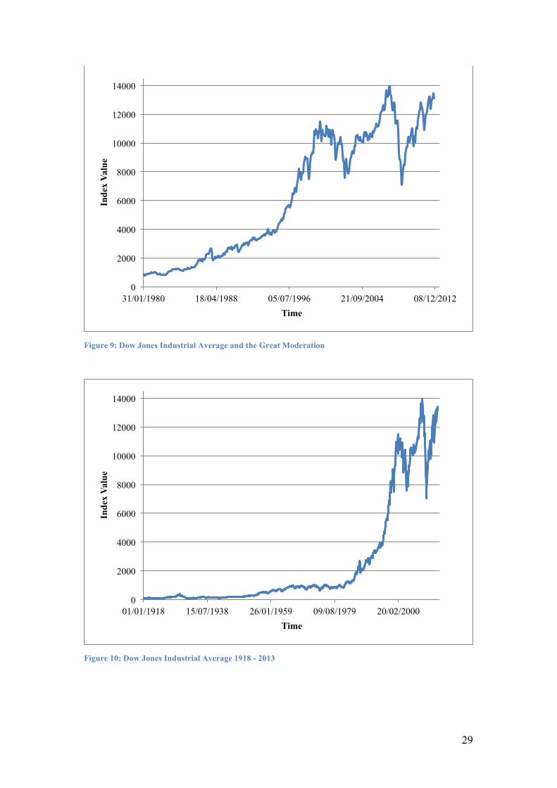
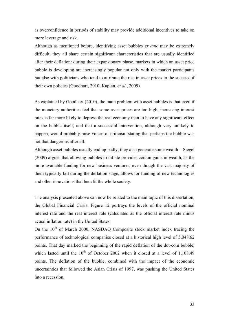
This spirit of optimism about the future was also present in the stock market. Figure 9
provides an overview of the changes in the values of Dow Jones Industrial Average
market index since the 31st of January 1980. In the three decades leading up to the
Financial Crisis, the index grew in value from 875.75 points on the 31st of January
1980 to 14,164.53 points on the 9th of October 2007, an increase by a factor of more
than sixteen. The following example makes it much easier to appreciate how
significant and rapid this change was: the growth of the value of the index that
occurred between January 1918 and May 1985 was an increase by a factor of the
same value too. Figure 10 provides graphical representation of the changes discussed
above.
The natural question to ask at this point of the analysis is what exactly were the
changes in economic policy that had such a tremendous impact on the macroeconomic
environment.
Page 29
29
Figure 9: Dow Jones Industrial Average and the Great Moderation
Figure 10: Dow Jones Industrial Average 1918 - 2013
0
2000
4000
6000
8000
10000
12000
14000
31/01/1980 18/04/1988 05/07/1996 21/09/2004 08/12/2012
Inde
x Va
lue
Time
0
2000
4000
6000
8000
10000
12000
14000
01/01/1918 15/07/1938 26/01/1959 09/08/1979 20/02/2000
Inde
x Va
lue
Time
Page 30
30
As pointed out earlier, academics generally accept the fact that it was the
improvement of monetary policy and its tools that ultimately created the environment
in which the volatility of business cycle could have been dampened.
Summers (2005) points out that the most significant development associated with
monetary policy was the decision to make controlling the inflation a central bank’s
top priority. Low and stable inflation generally contributes to a more stable economic
environment, as firms’ uncertainties about the future are reduced, and so are nominal
distortions associated with taxation, and finally low and stable expected inflation
provides policy makers with much more flexibility in responding to unforeseen events
such as banking crises (Summers, 2005).
Figure 11 portrays the levels of inflation rates in the United States and in the United
Kingdom, and shows that throughout the majority of the covered period they did in
fact remain low and fairly stable.
Figure 11: Inflation Rates in the United States and in the United Kingdom 2000 - 2012
The new monetary policy framework adopted in early 1980’s is broadly known as
conventional monetary policy. As Joyce, et al. (2012), explain, it was based on
inflation targeting, a policy aimed at achieving low and stable inflation by changing
the short-term interest rate at which central banks provide money to the interbank
money market in a manner that can be approximated by Taylor Rule.
-0.5
0
0.5
1
1.5
2
2.5
3
3.5
4
01/01/2000 09/02/2004 19/03/2008 27/04/2012
Infla
tion
Rat
e
Time
US Inflation
UK Inflation
Page 31
31
With the changes in the rate of inflation associated primarily with the extent of the
output gap, that is the difference between the current and the equilibrium level of
output, under this new monetary regime, a central bank would raise its official rate of
interest when inflation was predicted to increase above a fixed target level, and would
lower the interest rate if inflation rate fell below the target - all of the aforementioned
variables are incorporated into Taylor Rule, which in practical terms underpinned the
interest rate setting framework of monetary authorities (Goodhart, 2010).
Michael Woodford’s opus magnum, “Interest and Prices: Foundations of a Theory of
Monetary Policy” (2003), provides a very detailed theoretical framework upon which
conventional monetary policy was based, however, given the thoroughness of his
work, a detailed discussion of his contribution would go far beyond the scope of this
dissertation, and therefore it is only briefly summarised in this chapter.
Following the collapse of the Bretton Woods system of fixed exchange rates, the
value of money stopped being connected to any real commodity, creating a system of
fiat money, with its value depending only on the policies adopted by monetary
authorities (Woodford, 2003). To achieve greater macroeconomic stability, central
banks have committed themselves to explicit objectives concerning inflation, which
increased their ability to control it and brought increased price stability, providing
a strong foundation for economic growth (ibid.). Furthermore, by making their
policies more reliable and understandable for the private sector, abandoning the more
discretionary ad hoc system in favour of a more systematic and rule-based approach,
monetary authorities contribute to an increasing stability of the general economy
(ibid.).
Essentially, as explained above, Woodford (2003) presents a model in which the
monetary authorities can set their official nominal interest rate by standing ready to
lend and to borrow at their policy rate, allowing the quantity of money in the system
to be adjusted by arbitrage, rather than by using any specific quantity targets. His
work puts a particular emphasis on the fact that the policy adopted by a central bank
should be robust enough to prevail over a wide variety of random shocks to the
economy, rather than rely on models that consider only one type of shocks more
significant in importance than others (ibid.).
Page 32
32
The statement above, however, suffers from one fallacy, identified by Green (2005) –
Woodford’s theory considers credibility and commitment the two probably most
important features of conventional monetary policy but fails to offer a solution to the
problem of dealing with policies that may generate some desirable immediate effects,
yet may prove to be either unfeasible or harmful in the long-run.
Nonetheless, he still argues that Woodford’s work can be regarded “a bible for central
bank economists” (Green, 2005: p. 121), as it offers a theoretical framework that is
robust enough to derive an optimal policy matching a wide range of preferences and
opinions displayed by central bankers, such as in the case of differing views on
defining stability in terms of price level or in terms of inflation rate (Green, 2005).
The theory presented by Woodford (2003) overcomes a number of issues associated
with the previous system developed under neoclassical synthesis theoretical
framework, which assumes that the economy is Keynesian in the short-run and
classical in the long-run (Farmer, 2012), most importantly, it explains that
stabilisation policy, previously deemed ineffective due to the fact that shocks to
demand were assumed to be less significant in their importance than supply and
technology shocks, can be successful in suppressing the business cycle while also
providing additional welfare benefits (Green, 2005).
Despite its theoretical elegance and simplicity, and success in achieving low inflation,
as pointed out by Joyce, et al. (2012), conventional monetary policy suffers from one
significant setback – it does not prevent asset market bubbles from occurring, and
while it is true that it is difficult to identify and contain an asset bubble ex ante, the
soundness of the policy to allow a bubble to burst and then contain its negative effects
rather than to attempt suppressing its development remains highly questionable.
During a dinner speech on the 5th of December 1996 Alan Greenspan, then the
chairman of the Federal Reserve, famously said that, “We as central bankers need not
be concerned if a collapsing financial asset bubble does not threaten to impair the real
economy, its production, jobs, and price stability” (Shiller, 2005).
Goodhart (2010) points out to the fact that conventional monetary policy led to
a popular assumption that as long as central banks maintain macroeconomic stability,
the efficient financial markets will ensure financial stability, however, as pointed out
by Minsky (2008), more frequently the former may have inverse effects on the latter,
Page 33
33
as overconfidence in periods of stability may provide additional incentives to take on
more leverage and risk.
Although as mentioned before, identifying asset bubbles ex ante may be extremely
difficult, they all share certain significant characteristics that are usually identified
after their deflation: during their expansionary phase, markets in which an asset price
bubble is developing are increasingly popular not only with the market participants
but also with politicians who tend to attribute the rise in asset prices to the success of
their own policies (Goodhart, 2010; Kaplan, et al., 2009).
As explained by Goodhart (2010), the main problem with asset bubbles is that even if
the monetary authorities feel that some asset prices are too high, increasing interest
rates is far more likely to depress the real economy than to have any significant effect
on the bubble itself, and that a successful intervention, although very unlikely to
happen, would probably raise voices of criticism stating that perhaps the bubble was
not that dangerous after all.
Although asset bubbles usually end up badly, they also generate some wealth – Siegel
(2009) argues that allowing bubbles to inflate provides certain gains in wealth, as the
more available funding for new business ventures, even though the vast majority of
them typically fail during the deflation stage, allows for funding of new technologies
and other innovations that benefit the whole society.
The analysis presented above can now be related to the main topic of this dissertation,
the Global Financial Crisis. Figure 12 portrays the levels of the official nominal
interest rate and the real interest rate (calculated as the official interest rate minus
actual inflation rate) in the United States.
On the 10th of March 2000, NASDAQ Composite stock market index tracing the
performance of technological companies closed at a historical high level of 5,048.62
points. That day marked the beginning of the rapid deflation of the dot-com bubble,
which lasted until the 10th of October 2002 when it closed at a level of 1,108.49
points. The deflation of the bubble, combined with the impact of the economic
uncertainties that followed the Asian Crisis of 1997, was pushing the United States
into a recession.
Page 34
34
The reaction of the Federal Reserve to the worsening economic conditions was largely
consistent with the framework of conventional monetary policy – increasing the
interest rate when the economy is in a boom period and risks overheating, and
decreasing it, that is applying easy money policy, when there is a real possibility of
a recession (Siegel, 2009).
Figure 12: Official Nominal Interest Rate and Real Interest Rate in the United States
As presented in Figure 12, the Federal Reserve increased its official nominal interest
rate in the run up to the deflation of the dot-com bubble, trying to minimalize the
effects that its burst might have on the overall economy (preparing it for a soft
landing), and then, to stimulate recovery and growth, it switched from the tight to
easy money policy, lowering the interest rate from 6.5% to 1%.
The actions of the Federal Reserve had two profound effects: first of all, lowering
interest rates and flooding market with liquidity allowed to curb the ongoing
recession, which lasted only eight months, from March to November 2001; second,
and more importantly, by keeping the official interest rate at 1% until April 2004,
almost three years after the end of the 2001 recession, the Federal Reserve made
a significant contribution to the excessive growth of the mortgage market and to the
formation of another asset bubble, the housing market bubble.
-2
-1
0
1
2
3
4
5
6
7
01/01/2000 27/09/2002 23/06/2005 19/03/2008
Inte
rest
Rat
e
Time
FED Target Rate
US Real Interest Rate
Page 35
35
Goodhart (2010) states that central bankers tend to be very sensitive about the fact
that, at least in the past, their solution to a market crash was to cut interest rates
aggressively and persistently, thus encouraging a formation of a new asset bubble.
This strategy of adopting easy money policy as a response to a financial crash, in
order to prevent a recession or freezing up of a market, was also used in October 1987
in the wake of an unprecedented one-day 22% decline of the U.S. stock market with
no threat of a subsequent recession or further turmoil (Siegel, 2009).
In his paper, Siegel (2009) quotes the example of the infamous Gordon Gekko,
a rogue trader depicted in the 1987 film “Wall Street”, who used to say that greed is
good. He argues that out of all private vices, it is greed that makes the engine of the
economy hum, as people acting in their own interest, rather than pretending to act in
someone else’s, are encouraged more to channel their own vices to produce some
benefits, however, at the same time he points out that this process fails once its
participants begin to think that they are protected in one way or another from the
negative consequences that might arise while still being allowed to keep their reward
(Siegel, 2009).
The argument goes even further suggesting that the whole economic system
established after the conclusion of the Second World War provided a widespread
misperception about the responsibility and the ability of the government to foster
economic growth, occasionally intervening to counteract a recession. Siegel (2009)
explains this statement using four examples of government intervention policies, two
of which were already discussed in this chapter, i.e. the ability of the government to
foster the Great Moderation by skilful manipulation of the money supply, and its
ability to counteract the painful consequences of an asset market crash by flooding it
with liquidity.
The other two examples are those of the Great Depression, and the Great Inflation.
Friedman and Schwartz (1963) pointed out that the Federal Reserve bears
a significant proportion of the blame for turning the Black Tuesday Wall Street Crash
of October 1929 into the Great Depression by severely restricting the money supply
between 1929 and 1933, pursuing a policy of cripplingly tight money in the time of
collapsing real output. An extensive programme of Keynesian deficit spending
Page 36
36
policies, introduced by the Hoover and the Roosevelt administrations, as part of the
New Deal came to the rescue of the economy (even though economic historians agree
that the New Deal might have worsened the Depression, and it was the Second World
War that brought the United States out of it), and so, many people believe that if the
government managed to get the economy out of the Great Depression through fiscal
stimulation, it is capable of fixing any other significant economic problem (Siegel,
2009).
As far as the Great Inflation is concerned, it was caused primarily by an oil embargo
imposed on the United States by the Organisation of Arab Petroleum Exporting
Countries in 1973. With oil being an input to the U.S. economy of such a crucial
importance that a significant increase in its price would push it into a deep recession,
the Federal Reserve decided to rapidly expand the money supply to avoid it, which
resulted in inflation rates reaching 13.3% (Siegel, 2009). The Great Inflation came to
an end with the appointment of Paul Volcker as the chairman of the Federal Reserve –
although it pushed the economy into a recession in 1979 and another one in 1981 –
1982, his decision to sharply increase the interest rates brought the inflation down to
the manageable level of 3.9% (ibid.). Once again, modern macroeconomic policy
proved that it is capable of dealing with yet another threat to the stability of the whole
economy.
To summarise, the misguided lesson that seems to have been learnt from the four
aforementioned events is that the government has the ability and the means to solve
almost any economic problem through either fiscal or monetary intervention (Siegel,
2009).
Kaplan, et al. (2009) pointed out that greed and misaligned incentives, so typical of
human nature, lie at the heart of all asset bubbles. The erroneous perception of the
disappearance of fundamental macroeconomic risk factors associated with business
cycle fluctuations and inflationary threats, as well as the financial innovations
designed to reduce risk were, rather ironically, the means by which the risk of the
occurrence of an event as disastrous as the Global Financial Crisis was greatly
magnified (ibid.).
Page 37
37
Chapter III Post-crisis Macroeconomic Environment
So far, the analysis presented in this dissertation focused primarily on the causes of
the Global Financial Crisis, with the more immediate issues of a more financial nature
discussed in Chapter I, and its macroeconomic roots that contributed to the creation of
an imbalanced economic environment analysed in Chapter II. The discussion
presented in this chapter offers insights into the characteristics of the current post-
crash macroeconomic situation, which renders many of the conventional policy tools
ineffective, contributing to the ongoing weak and fragile recovery.
Before it discusses the aforementioned issue, however, the analysis will offer some
insights into the debate that immediately followed the Crisis, which questioned the
validity of the Efficient Market Hypothesis, and the rationale behind the economic
pretence of knowledge syndrome.
Throughout his book, Stiglitz (2010) actively criticises the view that the markets are
efficient and self-correcting, quoting many examples of their inefficiency that he
observed in the years leading up to and directly following the Global Financial Crisis.
Davies (2010) takes a similar position blaming the supposedly flawed Efficient
Market Hypothesis for the discrepancy between asset prices and economic
fundamentals, and even criticising business schools for their emphasis on short-term
returns and neglecting of ethical principles.
Zingales (2010), on the other hand, presents an argument which the author of this
dissertation finds much more well-balanced and easy to agree with. His paper argues
that the most recent market crash is much easier to explain in terms of the Efficient
Market Hypothesis than, for example, the October 1987 crash, when the market
dropped 22.6% in just one day with no major news or signs which could signal its
imminent collapse (Zingales, 2010).
The starting point of his argument is the one developed by Friedman, stating that
when there is a discrepancy between asset prices and their fundamental values,
a rational investor can profit by selling the overvalued one and buying the
undervalued one, with the very act of arbitrage trading pushing both prices towards
Page 38
38
equilibrium (Friedman, 1953). Zingales (2010) argues that the participants in the
housing market, however, are not smart investors trying to make the best use of the
discrepancy between prices and fundamentals described by Friedman, and that there is
a very high cost of arbitrage in this particular market. Nonetheless, despite the fact
that the asset-backed securities based on mortgages issued to the riskiest group of
borrowers were still considered safe, which with the benefit of hindsight seems rather
irrational, they were still priced correctly, which provides evidence that although they
were not perfect, markets remained efficient (ibid.).
Although it is fair to say that with irrational exuberance and lack of capital for smart
arbitrageurs, the Efficient Market Hypothesis is not strictly true, it still serves as
a sufficiently close approximation of the reality – what the Global Financial Crisis
really changed in terms of the Hypothesis, is the academic appreciation of how costly
the violations of the Hypothesis can be, particularly with significant leverage involved
(ibid.).
Stiglitz (2010) and Davies (2010) use one more argument against the theory of market
efficiency, pointing out the fallacy that the supporters of the market efficiency theory
exhibit by criticising the deflationary intervention of the Federal Reserve in the
markets, as, in their view, markets are currently unable to correct themselves.
Zingales (2010), however, provides a counterargument, in which he explains that the
supporters of Efficient Market Hypothesis do not in fact claim that the market always
gets it right and is able to correct itself, but that the cost of deviation from the efficient
state is incomparably lower than the cost imposed by a misguided interventionist
policy.
In essence then, the Global Financial Crisis cannot serve as an example of a fallacy of
the Efficient Market Hypothesis, but remains as a painful example of the potential
costs that deviations of asset prices from their fundamental values can have on the real
economy.
The phrase “pretence of knowledge” was coined by F.A. von Hayek, and was used as
the overarching idea in his Nobel-prize acceptance lecture:
“Of course, compared with the precise predictions we have learnt to expect in the
physical sciences, this sort of mere pattern predictions is a second best with which one
does not like to have to be content. Yet the danger of which I want to warn is
Page 39
39
precisely the belief that in order to have a claim be accepted as scientific it is
necessary to achieve more. This way lies charlatanism and worse. To act on the belief
that we possess the knowledge and the power which enable us to shape the process of
society entirely to our liking, knowledge which in fact we do not possess, is likely to
make us do much harm” (Hayek, 1989: p. 7).
This statement seems to be particularly applicable in the post-Crisis situation in which
we currently are. After all, as mentioned in Chapter II, many prominent
macroeconomist shared the seemingly justified belief that the long and stable growth
associated with the Great Moderation would carry on in the foreseeable future with
a minimal risk of recessions, which modern macroeconomic policy tools were
supposed to prevent so well.
Caballero (2010) argues that, taking into account that the ultimate goal of
macroeconomics is to explain and model the aggregate outcomes stemming from the
decisions of multiple economic agents interacting through a number of complex
markets, addressing this extremely ambitious goal in an adequate manner, preferably
displaying microeconomic-theory-like precision, is incredibly difficult. One approach
to the problem is to abandon the attempts to formalise economic theories in
mathematical terms incapable of capturing the complexity of the world they try to
explain, whereas the other, one that modern macroeconomics seem to prefer, is to
develop a number of methods allowing to portray a precise yet irrelevant world in
a highly quantitative manner (Caballero, 2010).
The problem with designing an effective macroeconomic policy tool, however, is that
by their very nature, crises are unpredictable, for otherwise they would not be capable
of causing such a high degree of instability and turmoil, and for this reason, the
probability of designing a policy capable of offering more than some common-sense
procedures is rather low (ibid.).
To conclude, it is probably fair to say that the pre-Crisis macroeconomics framework
displayed highly developed syndromes of Hayekian pretence of knowledge, however,
one should hope that the lessons we have learnt from the Crisis will help us realise
how little we really know, which in turn will stimulate our desire for better and more
accurate theories.
Page 40
40
In its latest “Economic Outlook” the Organisation for Economic Cooperation and
Development (2012) summarised the current macroeconomic situation emphasising
the following facts:
1. Recovery is projected to be hesitant and uneven over the next two years, with
the European Monetary Union remaining in close-to-recession conditions for
the foreseeable future;
2. Given the weak economic outlook, accommodative monetary policy is still
required, with further easing necessary in the European Monetary Union;
3. Fiscal consolidation is necessary in many countries but, given high fiscal
multipliers at the moment, excessive austerity might prove to be very costly;
4. Lower interest rates, further quantitative easing, and additional policy support
will be necessary should serious downside risk materialise;
5. The crisis in the European Monetary Union remains the greatest threat to the
global economic recovery, in spite of the recent policy adjustments that have
resolved its immediate problems – much more still remains to be done to
ensure long-term stability.
Because of the complexity and the breadth of the issues identified above, a very
detailed and insightful analysis would require far more attention and research than the
scope of this dissertation is capable of offering, even though it would provide an
overarching perspective on the whole cause and effect chain of the events set in
motion by the inflation of the asset bubble in the American housing market. For this
reason, the discussion presented in this chapter will focus primarily on providing an
overview of the changes in fiscal and monetary environment that forced the policy
makers to abandon their traditional macroeconomic tools.
Barrell and Holland (2010) provide a very concise, yet accurate explanation of the
main source of the current extremely difficult monetary and fiscal environment – as
the liquidity crisis in the banking sector grew in scale to the extent that it finally
transformed into a large-scale solvency crisis, it became increasingly clear that the
central banks would not be able to act as the lender of last resort, due to their inability
to lower their official interest rates any further. That meant that the government would
have to step in, increasing its budget deficit in order to provide emergency funding for
the banking system. Furthermore, as pointed out by Reinhart and Rogoff (2009a), the
Page 41
41
inevitable collapse of tax revenues that the governments suffer from in the wake of
deep and prolonged crises, and the ambitious countercyclical fiscal policies that they
have adopted, were the additional drivers of increasing national debts.
The first step in the analysis of the post-Crisis macroeconomic environment presented
in this chapter is the analysis of the monetary environment in which conventional
monetary policy, described in the previous chapter, is rendered ineffective.
A good starting point of the discussion is the IS – LM model developed as
a mathematical formulation of the ideas presented by John Maynard Keynes (1973) in
“General Theory of Employment, Interest, and Money”.
The IS (Investment and Saving) side of the model captures the effects of changes in
interest rates on aggregate demand, whereas the LM (Liquidity preference and Money
supply) depicts the equilibrium in the money market for a given level of money
supply (Begg, et al., 2008). The model was formulated primarily by John R. Hicks in
1936, and is based upon the following set of equations:
𝐼𝑆:𝑌 = 𝐶 𝑌 − 𝑇 + 𝐼 𝑟 + 𝐺; 𝐿𝑀:!!= 𝐿(𝑟,𝑌)
where: Y – income/output, C – consumption, T – taxes, I – investment,
G – government spending, M – money supply, P – price level, L – liquidity
preference, r – interest rate.
As lower interest rates increase both aggregate demand and output, the IS schedule
line has a negative slope – changes in the rate of interest cause movements along the
IS line, whereas any other changes in aggregate demand shift the line in one direction
or another (ibid.). Figure 13 provides a graphical representation of the IS schedule.
As far as the LM schedule is concerned, it has a positive slope, as, given that money
supply is assumed to be fixed, only an increase in interest rates can counteract the
effects of greater quantity of money demanded resulting from higher income, bringing
the money market back to equilibrium state (ibid.). Figure 14 below depicts the LM
schedule.
Page 42
42
Figure 13: The IS Schedule
Figure 14: The LM Schedule
With the two halves of the model combined, the IS-LM model becomes a general
equilibrium model depicting the equilibrium interest rate r* that brings both the goods
Income
Inte
rest
Rat
es
I-S
r(2)
Y(2)
r(1)
Y(1)
Income
Inte
rest
Rat
es
L-M
r(1)
(r(2)
Y(1) Y(2)
Page 43
43
market and the money market into equilibrium, resulting in the equilibrium level of
income Y* (ibid.). The complete IS – LM model is portrayed in Figure 15 below.
Figure 15: General Equilibrium in the IS - LM Model
As indicated in Chapter II, the neoclassical synthesis theoretical framework assumes
that the economy is Keynesian in short-term and classical in the long-term (Farmer,
2012), therefore applying the IS – LM model to analyse some of the ongoing
macroeconomic problems might prove particularly helpful.
One particular problem exhibited by the model was described by one of its authors,
merely a year after it was finally formulated – Hicks (1937) noticed that under severe
economic distress conditions, the LM schedule line will become flatter near its left-
hand end, which means that shifting it by increasing the quantity of money supplied
will have no effect on equilibrium interest rate and income, as shown in Figure 16.
Income
Inte
rest
Rat
es
I-S
L-M
r*
Y*
Page 44
44
Figure 16: The problem of the IS - LM Model6
This particular problem is known as the liquidity trap – the fact that, in words of
Hicks, turns the “‘General Theory of Employment’ into Economics of Depression”
(Hicks, 1937: p. 155), as monetary policy becomes completely ineffective. Krugman
(2000) explains the problem using a simple example – if we assume that bonds and
money are effectively assets that can be considered perfect substitutes, which they
become if interest rates are very close to zero, then conventional monetary policy, in
which bonds are swapped for money in open-market operations, does not change
anything.
Although monetary authorities can no longer employ the conventional policy tools in
liquidity trap conditions, they can still opt for a policy which has the potential to solve
the problem – a credible commitment to achieving inflation rates higher than the
target-rate under normal economic conditions, which will lower the real interest rate
and stimulate the economy out of liquidity trap despite the nominal interest rate
remaining at a near-zero level (Jeanne and Svenson, 2007). The problem, however, is
that making a credible commitment to higher future inflation rates may be difficult to
achieve, as investors may expect the central bank to change its policy target rate back
6 Figures 13 – 16 used to explain the IS – LM model are author’s own work.
Income
Inte
rest
Rat
es
r*
Y*
I-S
L-M (1) L-M (2)
Page 45
45
to the initial one once economic conditions improve (ibid.). To overcome this
problem, Jeanne and Svenson (2007) recommend a strategy of central bank’s capital
management, in which capital levels are reduced to the minimum that would be
consistent with a future exchange rate associated with the desired higher inflation rate,
thus providing a more credible commitment to increasing inflation. This approach,
however, has been criticised by Sims (2004) for minimising the central bank’s
potential to avoid a self-fulfilling hyperinflation threat.
In the midst of the Crisis, the lending in the interbank markets as well as lending to
consumers came to a sudden halt, as banks began accumulating cash on their balance
sheets having they lost their confidence about the future, pushing the economy into
a liquidity trap (Skidelsky, 2011).
The countercyclical monetary policy, described in more detail in the previous chapter,
relied heavily on its ability to flood the market with liquidity in times of financial
crises and recessions in order to first stabilise it and then stimulate economic recovery
and growth, however, having sharply lowered the official nominal interest rate from
5.25% in 2007 to 0.25% in late 2008 in the United States, and from 5.75% in 2007 to
0.5% in mid-2009 in the United Kingdom, to little or no real effect, the monetary
authorities found themselves in a situation, whereby they were simply unable to
stimulate the economy any more, due to the fact that the official interest rates could
not be decreased any further (Buckley, 2011). Conventional monetary policy had to
be abandoned – credit easing and quantitative easing, the unconventional monetary
policies that replaced it, are described in much more detail in Chapter V.
The Austrian School of Economics, on the other hand, provides an alternative
explanation of the lack of any significant impact on output that monetary policy
displays under near-depression conditions. Mises (1996) suggests that artificially
induced periods of economic boom encourage overconsumption and malinvestment,
which leads to a misallocation of the scarce factors of production with a simultaneous
reduction of available stocks. In his view, a recession, or in the worst-case scenario,
a depression always follows an economic boom, so consumption can return to its
natural state, and factors of production can be reallocated back to the industries which
use them the most efficiently (Mises, 1996). In essence, economic downturn brings
about forced saving and forced liquidations, which ultimately restore the initial
Page 46
46
economic balance (Garrison, 2004). Mises (1996) points out, however, that
a government intervention aimed at aiding the failing industries, which benefited from
the malinvestment the most, will only prolong the period of economic downturn, as it
protects them from liquidation, thus not enabling the market to return to its
equilibrium state while enforcing the cost of this prolonged agony on the taxpayers.
This line of thought suggests that lowering interest when economic growth slows
down results only in allowing the firms that are bound to fail, as the market attempts
to correct malinvestments, to avoid liquidation for much longer than necessary –
ultimately, by lowering its official interest rate as much as it can, a central bank
prevents the market forces from restoring the balance, creating liquidity-trap-like
conditions, in which it cannot conduct its conventional policy anymore, while the
economy still remains in recession.
Having established that the monetary authorities, facing a liquidity trap, had to
abandon their typical tools and policies in favour of unconventional policy, the
analysis will now focus on fiscal policy. As mentioned before, due to collapsing tax
revenues and substantial countercyclical programmes, governments of the countries
most affected by the Global Financial Crisis have been facing increasing levels of
debt. Skidelsky (2011) points out that as the Crisis deepened, governments intervened
in almost every single market with various forms of stimulus packages including
bailouts, tax rebates, printing money, subsidies for private businesses, and other forms
of debt-financed public spending, which most economists and policy-makers are
calling for withdrawal from, as they fear that carrying on with this policy may lead to
governments going bankrupt, high inflation, or both.
As a result of the Crisis the gross government debt levels have increased by 30
percentage points between 2007 and 2011 in advanced economies, reaching 103% of
GDP in the United States, 230% of GDP in Japan, 83% of GDP in the United
Kingdom, and 88% of GDP in the European Monetary Union (Bussiere, 2013).
Figure 17 portrays the rising levels of indebtedness of several European countries
between 2000 and 2011, and provides a graphical representation of the direness of
their fiscal situation.
Page 47
47
Figure 17: Public Debt as Percentage of the GDP 2000 - 2011
Ghosh, et al. (2013) point out that the currently observed public deficits and primary
balances of the advanced economies have reached their highest levels in the last 40
years, and furthermore, that the sharp increases of their borrowing costs, from
essentially risk-free rates to the levels considered prohibitively costly implying an
increasing risk of possible insolvency, should serve as a warning sign to other
countries at risk of exhausting their fiscal space.
Typically, a responsible government increases its primary surplus in response to rising
debt service in order to maintain a constant debt-to-GDP ratio at a reasonable level,
however, a large economic shock, for example a war or a financial crisis, may force it
to temporarily abandon the aforementioned policy, only to increase the primary
surplus again in the future to offset the higher interest bill (ibid.).
Increasing the primary balance enough to offset the interest bill, however, may not be
possible under certain circumstances, as at sufficiently large levels of debt, the
primary balance would have to exceed the gross domestic product – if the primary
balance displays fiscal fatigue, that is it fails to keep up with the increasing debt
service, there is the possibility that the government will have to default having
reached sufficiently high debt level (ibid.). The main problem is that the risk premium
0
20
40
60
80
100
120
140
160
180
Deb
t Per
cent
age
of th
e G
DP
Time
Greece
Ireland
Italy
Portugal
France
Germany
UK
Page 48
48
a government has to pay on its debt increases together with its indebtedness, so after
reaching a certain level of debt, the risk of government default becomes self-
propelling, as higher levels of debt imply higher risk premium, which in turn
increases the borrowing costs leading to even higher levels of debt, etc. (ibid.). Once
a government finds itself in this loop, as suggested by Arellano (2008) and Mendoza
and Yue (2012), it faces a decision of whether or not to default, which is ultimately
based upon the balance of gains resulting from avoiding at least a proportion of its
debt service obligations, against the costs of output losses and restricted access or
even exclusion from international credit markets.
With the increasing risk of exhausting their fiscal space, understood as the scope that
policy-makers have to calibrate fiscal policy without facing the risk of reaching
unsustainable debt levels (IMF, 2012), governments had to adopt austerity measures
and consolidation efforts aimed at bringing their debt-to-GDP ratios back to
manageable levels, particularly given the pressure from the financial markets reacting
particularly badly to even the slightest hint that yet another country might be facing
insolvency.
The most significant problem with fiscal consolidations centres around their duration,
composition, that is whether they are spending or tax based, and the public’s
expectations of their composition (Bi et al., (2013)). Research suggests that when
people anticipate tax increases used as one of the imminent austerity measures, they
will suffer from higher inflation and higher debt service costs, even if the
consolidation programme turns out to be spending based (ibid.). Moreover, the
perception of undesirable fiscal consolidation may have a negative impact on overall
economic activity, as distortionary taxation may increase marginal costs and fuel
inflation, whereas substantial spending cuts implemented too quickly and too
extensively may lead to increasing deflationary pressures (ibid.).
Interestingly enough, Bilbiie et al. (2013) report that debt financed tax cuts may have
a rather paradoxical consequence: due to redistribution effects shifting wealth from
savers to borrowers when a tax cut is implemented, followed by another redistribution
in the opposite direction when taxes are increased in the future in order to repay the
debt, borrowers have the incentive to work less, whereas savers, to work more, which
ultimately leads to an overall contraction in spending and output – essentially, a tax
Page 49
49
cut today may result in economic contraction, and a tax increase in the future may
lead to economic expansion, primarily because debt-financed tax cuts increase the
aggregate spending of borrowing-constrained agents who will be forced to consume
less once the economy reaches its steady-state and taxes are increased.
It is also worth mentioning the findings presented by Corsetti, et al. (2013), who
reported that pessimistic expectations about the future, regardless of whether they are
related to any fundamentals, cause upward revisions of deficits, increasing risk
premiums, which in turn increase private borrowing costs, ultimately contributing to
a deceleration of economic activity. This self-fulfilling expectation is particularly
apparent when the risk of sovereign default is very high and the monetary policy is
constrained, as monetary authorities cannot lower the official interest rate to
counteract the expected negative developments (ibid.).
As reported by the International Monetary Fund (2012), the deficits of advanced
economies decreased by one percentage point in 2012, although countries with more
fiscal space, like Germany and Canada, should consider slowing the pace of their
consolidation programmes to avoid excess fiscal contraction that has the potential to
further deteriorate the current economic conditions – this short-term caution, however,
should not serve as an excuse to limit the efforts to put the public finances in order,
which remains a key requirement for a more sustainable economic growth in the
future. The importance of fiscal tightening programmes becomes particularly apparent
when the fact that central banks currently hold large amounts of government debt and
other assets, which will have to be liquidated or rolled over to the private sector one
day in order to bring the monetary base back to its original state, is taken into account
(ibid.).
The debt levels are expected to stabilise by 2015, however, due to delayed effects that
fiscal policy has on the real economy the importance of communicating government
strategies to general public in order to fuel confidence and credibility of its actions
cannot be overemphasised (ibid.).
The discussion presented above indicates how difficult designing an effective fiscal
policy is under conditions rendered by the current macroeconomic environment.
Taking into account that monetary policy is significantly constrained by effectively
reaching the zero lower bound on interest rates, managing expectations of the public
Page 50
50
becomes really important. Implementing a fiscal consolidation programme that is too
severe or attempts to reduce the debt-to-GDP ratio too quickly may have adverse
effects on expected economic growth. A programme that is not extensive enough, on
the other hand, may result in increased borrowing and debt service costs that can
further hinder the already weak economic recovery. There is a fine balance between
the two approaches and the governments of the advanced economies affected by the
Crisis the most face a very difficult task of getting it right in the early stages of
implementing fiscal tightening measures.
Page 51
51
Chapter IV The Unique Experience of Japan
Despite having led the global economic growth in the 1960’s and the 1970’s,
maintaining a very strong position during the 1980’s, the Japanese economy has
remained in an economic stagnation ever since (Tyers, 2012). The Japanese financial
crisis that began in 1992 bears a striking resemblance to the Global Financial Crisis,
both as far as its causes and the responses of the policy-makers are concerned
(Reinhart and Rogoff, 2009b) – with the Japanese experience of two “lost decades”, it
is definitely worth taking a closer look at the origins and the consequences of the
problem, as the benefit of hindsight might provide some valuable lessons that will
allow not repeating the same mistakes and facing similar prospects of the future.
The analysis begins with providing a brief overlook of the Japanese economy over the
last thirty years, setting the stage for further discussion presented in this chapter.
Figures 18 – 20 depict the changes in growth rates of the Japanese gross domestic
product, the changes in the official nominal rate of interest of the Bank of Japan, and
the changes in the value of the main Japanese stock market index, Nikkei 225.
Figure 18: Gross Domestic Product Growth in Japan 1980 - 2012
-20
-15
-10
-5
0
5
10
15
01/09/1980 01/09/1987 01/09/1994 01/09/2001 01/09/2008
Gro
ss D
omes
tic P
rodu
ct G
row
h R
ate
Time
Page 52
52
Figure 19: Bank of Japan Official Interest Rate 1980 - 2012
Figure 20: Nikkei 225 Performance 1980 - 2012
There a number of issues that become immediately apparent after taking a closer look
at the data depicted in Figures 18 – 20. First of all, as mentioned in the introduction to
-2
0
2
4
6
8
10
01/01/1980 19/03/1988 05/06/1996 22/08/2004 08/11/2012
Inte
rest
Rat
e
Time
0
100
200
300
400
500
600
700
01/01/1980 19/03/1988 05/06/1996 22/08/2004 08/11/2012
Cha
nge
in In
dex
Valu
e (1
00 =
Initi
al V
alue
)
Time
Page 53
53
this chapter, the strong pattern of relatively economic growth rates changed in the
early 1990’s, deteriorating significantly. Second, the monetary policy pursued by the
Bank of Japan seems to closely resemble the pattern displayed by the interest rate
decisions of the Federal Reserve portrayed in Figure 12 in Chapter II, as the Japanese
interest rates were increased in the run up to the market crash, and then sharply
decreased, almost to zero in the aftermath. Interestingly enough, the apparent lack of
data for the period between early 2001 and early 2006 is not a result of a printing
error but a reflection of the fact that the Bank of Japan did not quote official interest
rate at all in that period. Finally, the Japanese stock market has never recovered from
the crisis, as the recent value of the Nikkei 225 Index is only 30% higher than the one
recorded in early 1980, which compared to the value it reached in the early 1990’s, an
increase by the factor of six in just ten years, is a fairly disappointing performance.
The academic debate that followed the meltdown of the Japanese economy,
reinvigorated by the more recent developments of the Global Financial Crisis,
identified a number of factors that pushed the economy into a recession followed by
stagnation. The most important ones include:
1. Japanese Yen appreciation enforced by the Plaza Accord;
2. Steady deterioration in the health of the banking system;
3. Deflation of the real-estate asset bubble.
Over the twenty two years between 1951 and 1973 the Japanese economy grew on
average by 9.2% per annum – with such an amazing record of economic growth,
while simultaneously running large current account surpluses, Japan was considered
by many a crisis-free economy (Itoh, 1994). The economic policy ran by the United
States at that time, on the other hand, involved combining significant budgetary
expansion, and high counter-inflationary interest rates, resulting in large trade deficit
and a higher value for dollar (Hamada and Okada, 2009).
The Plaza Accord was an agreement intended to restore the savings-investment
balance of the United States, signed in September 1985 in New York City by the
representatives of the Group of Five – France, Japan, the United Kingdom, the United
States, and West Germany – with an explicit aim of coordinating their policies in
order to cause a depreciation of the US dollar against other currencies, including the
Japanese yen (Fletcher, 2012). Prior to 1985 the fragile appreciation of the dollar
Page 54
54
against the yen was driven primarily by speculative monetary investment, which fell
sharply after the signing of the Plaza Accord (Itoh, 1994).
As a result, the yen appreciated dramatically while the Japanese economy was
simultaneously slowing down (Kusukawa, 1994). The Japanese industry took a full
advantage of the declining prices of raw materials and energy, resulting primarily
from decreasing energy prices combined with a cheaper price of imports, although the
positive effects of this stronger industrial performance were largely offset by the
increasing importance of services sector and rising costs of labour (ibid.). Medium
and small enterprises, however, less competitive internationally, were harmed by the
appreciation of the yen, and saw their profits decline rapidly with many forced into
liquidation (ibid.).
The increase in wealth associated with the appreciation of the yen, together with the
decision of the Bank of Japan to reduce its official interest rate from 5% in 1985 to
2.5% in 1987, resulted in faster growths in the Japanese stock exchange that began
accelerating in 1986 (Itoh, 1994). The private sector’s demand for traditional banking
services, loans and deposits, was decreasing, while the demand for more speculative
financing was on the rise (ibid.).
Although the Japanese stock market declined in response to the Black Monday on
Wall Street in October 1987, the monetary authorities remained reluctant to increase
interest rates for almost two more years (Kusukawa, 1994). The prices of real estate in
the meantime more than doubled between 1986 and 1988 (Itoh, 1994), and increased
by a factor of five by mid-1991 (Fletcher, 2012). The Bank of Japan’s easy money
policy also fuelled aggressive corporate speculative investments, while real
investments in capital remained small and stagnant (Itoh, 1994).
By early 1990, the Japanese monetary authorities realised that the economy is
overheating, and so, in order to prepare it for a soft landing, they began increasing the
official interest rate from 3.25% in May 1989 to 6% in August 1990 – the plan,
however, did not work, and the higher interest rate served as a catalyst only
accelerating the speed at which the asset bubble deflated (Fletcher, 2012).
Just like in case of any other asset bubble, the growth of prices in the Japanese real
estate market was expected to continue indefinitely, which encouraged the banks to
expand their mortgage facilities, offering loans based on 100% of the value of the
Page 55
55
property against which the mortgage was made (Kusukawa, 1994). Following the
collapse of the bubble, however, property prices declined, and with the quality of
mortgages deteriorating they became increasingly difficult to liquidate (Itoh, 1994).
With the total value of the bad loans held on banks’ balance sheets amounting to 7%
of the gross domestic product, Japan experienced its first bank failures in more than
40 years (Hoshi and Kashyap, 1999).
In an attempt to contain the situation, the Bank of Japan began lowering its official
interest rate in July 1991, reaching the level of 1.7% in September 1993 – the easy
money policy combined with a fiscal stimulus package of tax cuts and direct
government spending amounting to $430 billion, was supposed to provide emergency
liquidity and stabilise the market (Kusukawa, 1994). Furthermore, the government
established a number of institutions charged with the task of addressing the issue by
buying bad loans, nationalising the most endangered banks, reorganising the banking
supervision system, and providing ¥60 trillion for reorganisation and recapitalisation
of banks, with further ¥7.5 trillion for emergency bailouts (Hoshi and Kashyap, 1999).
Despite further attempts to provide fiscal and monetary stimulus to the economy,
including lowering the official interest rate to exactly 0%, between 1990 and 2003
gross domestic product grew on average by 1% per year (Fletcher, 2012).
A number of other factors, more specific to the Japanese banking system and its
corporate culture, played an equally important role in the escalation of the Japanese
crisis.
Kanaya and Woo (2000) point out that the crisis was facilitated by regulatory
weakness of the banking system, as the financial authorities, which had the power to
revoke a bank’s license, intervened only after the distressed institution had become
insolvent. Furthermore, the strict guidelines issued by the Tokyo Stock Exchange,
requiring delisting of a company which incurred losses for three consecutive years,
provided an incentive for the banks to manipulate their balance sheets in order to
provide proof of meeting that requirement (ibid.). Due to widespread practice of
paying low but consistent dividends to shareholders, regardless of financial
performance of a firm, banks were also allowed to continue paying dividends out,
even when it had become clear that the retained earnings would have helped
Page 56
56
improving their profitability and capital base (ibid.). Finally, the loan classification
rules, relatively lax compared to international best practice standards, failed to
provide an accurate assessment of the extent of existing bad loans (ibid.).
Miwa and Ramseyer (2002), on the other hand, argue that large Japanese firms
obtained almost all their funding from the decentralised, and highly competitive
capital markets, which ultimately allowed them to become hugely successful,
particularly in the case of zaibatsu firms, that is large groups of corporations working
together, which managed to accumulate enormous amounts of wealth and political
power.
As mentioned before, the attempts of the monetary authorities and the government of
Japan to stimulate economic growth by lowering official interest rates to the zero
lower bound and by injecting trillions of dollars into the economy through increased
government spending yielded hardly any results – over the thirteen years between
1990 and 2003, gross domestic product had grown by an average of 1% per year
(Fletcher, 2012).
Having reached the state in which monetary stimulation was no longer possible, the
Japanese economy found itself in a liquidity trap described by Krugman (2000).
In March 2001, the Bank of Japan decided to abandon conventional monetary policy
and opted for the use of unconventional monetary policy, quantitative easing. This
decision is reflected in Figure 19, by the period when the Bank did not quote any
official interest rate. A technical explanation of how quantitative easing works is the
main objective of the subsequent chapter, so for the purposes the comparative analysis
offered in this chapter, the discussion focuses primarily on the effectiveness of
quantitative easing in Japan.
Girardin and Moussa (2011) state that the new policy implemented by the Japanese
central bank had been successful, as it had a positive impact on economic activity and
prices. Furthermore, they argue that due to changes in regulatory environment
resulting in a firm commitment to clean the balance sheets of banks of toxic assets,
a purpose for which the Japanese government provided $460 billion, quantitative
easing is much more effective after the quality of assets held on balance sheets had
been improved.
Page 57
57
However, taking into account the decision of the Bank of Japan to launch the eighth
round of quantitative easing, announced on the 4th of April 2013, involving increasing
an injection of $1.4 trillion into the economy within the next two years (Kihara and
White, 2013), the arguments presented by Girardin and Moussa (2011) seem to be
fairly detached from the reality – after all, if quantitative easing had been successful
in stimulating economic growth in 2001, why would the Bank of Japan still use it as
its main policy tool, particularly providing monetary stimulus of an unprecedented
scale?
The comparative analysis between the Global Financial Crisis and the Japanese crisis
of the 1990’s seems to be quite justified and capable of shedding some light on the
effects that policies adopted as a response to the 2007 – 2009 Crisis might have on
economic recovery, given that both crises appear to have a fairly similar origin –
a real estate asset bubble, combined with excessive mortgage lending, and aggressive
financial speculation. Furthermore, the monetary authorities, both in the case of Japan
and in the case of the United States, can be blamed for fuelling the inflation of the
market asset bubble by keeping their official interest rates on a really low level for fat
too long, as well as for taking the steps resulting in a sharp burst of the bubble by
increasing the interest rates too aggressively.
The fiscal and monetary responses to both crises appear to be quite comparable as
well – both countries used a combination of fiscal and monetary stimulus, followed by
a switch to unconventional monetary policy, once the official interest rates reached
their zero lower bounds.
With so many matching elements of the Global Financial Crisis and the Japanese
crisis of the 1990’s, it is quite reasonable to ask the following question: are we too
facing a lost decade of weak recovery and fragile growth?
Page 58
58
Chapter V Unconventional Monetary Policy
Unconventional monetary policy, in particular quantitative easing, has already been
mentioned a number of times at various stages of the analysis presented in this
dissertation, however, it has not been explained and described in detail until this
Chapter. The relative uniqueness of this policy and the fairly limited body of existing
literature describing it in great detail, despite the difficulty it presents, make the
following analysis much more valuable in terms of academic research.
The term “unconventional monetary policy” is defined largely by what it is not, rather
than what it actually is – it might involve setting negative official nominal interest
rates, just like in case of Denmark, or expanding the central banks balance sheet
through a series of asset purchases (Joyce, et al., 2012). Although explicit quantitative
monetary targets were the main policy tool underpinning the monetary framework
until the early 1980’s, when it was abandoned in favour of conventional monetary
policy and its inflation targeting-based tools, as mentioned in Chapter IV, following
the failed attempts to stimulate the Japanese economy in the late 1990’s, the Bank of
Japan was forced to revert back to the regime of targeting quantitative monetary
aggregates, giving it a new name – quantitative easing (Lyonet and Werner, 2012).
The current macroeconomic situation in the developed Western countries closely
resembles the one characterising the Japanese lost two decades, and so the adaptation
of credit easing by the United States and quantitative easing by the United Kingdom
was only a matter of time.
The main problem for monetary policy in the period following the Global Financial
Crisis stems from the fact the official interest rates controlled by the monetary
authorities are constrained in their value by zero, as individual agents can always hold
on to non-interest bearing cash, even though the Taylor Rule approach might suggest
setting negative nominal interest rates (Joyce, et al., 2012). This particular problem
renders conventional monetary policy ineffective at the moment, as given the fact that
the nominal interest rate in the United Kingdom is already set at the level of 0.5%
Page 59
59
since March 2009, and the nominal interest rate in the United States is set at the level
of 0.25% since December 2008, the monetary authorities simply cannot lower their
official interest rates any further to provide more liquidity to the market and ease the
credit conditions in order to facilitate economic recovery. This situation represents
a classic, textbook-like example of liquidity trap, described in detail in Chapter III.
Conventional monetary policy theory described by Woodford (2003), emphasised the
importance of setting short-term nominal official rates of interest over the quantities
of money involved in open market operations used as the policy transmission
mechanism. As explained above, however, in the liquidity trap conditions, the
conventional monetary policy mechanisms cease to be effective and have to be
replaced by other tools and mechanisms.
Essentially, as explained by Joyce, et al. (2012), quantitative easing focuses primarily
on expansion of central bank’s balance sheet through asset purchases – with its ability
to create unlimited quantities of acceptable means of payment, the central bank is able
to buy a pre-specified amount of assets, be it government bonds or other types of
assets issued by the private sector. These purchases change the composition of the
portfolio of assets held by the private sector, with the final outcome resulting in
a smaller proportion of previously owned assets, now purchased by the central bank,
and a higher proportion of claims on the central bank, i.e. money (ibid.). Ultimately,
both assets and liabilities of the central bank, the latter most likely held in form of
reserves of the banking system, increase by the same amount.
Before the analysis moves further to discuss the transmission mechanism of
quantitative easing, it is necessary to explicitly state the assumptions under which the
policy might work. Eggertsson and Woodford (2003) established that under
conditions that are similar to Ricardian Equivalence, whereby the private sector is
indifferent between its own assets and the assets of the central bank or the
government, an exchange of the assets will have no real effect on the economy. This
fact was emphasised further in the paper by Joyce, et al. (2012), as they explicitly
expressed the fact that in order to generate any impact through quantitative easing,
portfolio switches have to make a difference for the investors.
Page 60
60
There are two main channels through which quantitative easing operates – the
portfolio substitution channel, and the bank funding channel. Figure 21 below
provides a graphical representation of those channels.
Figure 21: Quantitative Easing Operations Channels7
In the case of the Bank of England, as explained by Joyce, et al. (2012), the portfolio
substitution channel works in the following way:
1. The Bank purchases gilts, reducing their free float and increasing its reserves
held by commercial banks, as most of the proceeds from those sales show up
in bank deposits; since gilts and bank deposits are not perfect substitutes, the
exchange of assets affects the duration of portfolio held by investors, as the
swap of gilts for deposits is equivalent to trading a long-dated asset for a short-
dated one;
2. In order to rebalance the duration of their portfolios, some investors will use
the proceeds from the sale of their assets to buy another type of long-dated
assets;
3. By reducing the stock of privately owned long-dated assets, the Bank of
England lowers the duration risk which should result in lower premium
requirements, which combined with portfolio duration rebalancing result in
increases in prices of long-dated risky assets, most importantly, corporate
bonds and equities;
7 Joyce, et al. (2012), p. 278
Page 61
61
4. Higher prices of the assets mentioned above allow companies to raise funds
more easily, and also result in capital gains for households, increasing their
wealth, which in turn should lead to higher consumption or other form of
spending, ultimately increasing aggregate demand and output in the economy.
The other channel through which quantitative easing operates, bank funding channel,
is significantly less complicated and much easier to understand – as the central bank
purchases gilts owned by private investors, the amounts of money deposited at banks
increases, reflecting the proceeds from sales, as do the reserves held at the central
bank – once the level of reserves exceeds the demand for liquidity, banks will become
much more willing to expand their lending (Joyce, et al., 2012).
Having explained the design and transmission mechanisms of quantitative easing, the
analysis will now focus on assessing the impact that the policy had on the real
economy thus far, although taking into account the effects of quantitative easing on
stimulating growth in Japan, it is natural to be very sceptical about the potential for
stimulation the policy displays.
At this point, however, it is worth mentioning what the scale of the quantitative easing
in the United Kingdom and in the United States has been since the programmes were
initiated. In total, the Bank of England created additional £375 billion in three rounds
of quantitative easing (Bank of England, 2013). It is much more difficult to assess the
amount of new money created by the Federal Reserve, as its credit easing programme
has explicit monthly quantity targets, unlike the British one with target amount
specified for each round of stimulation. Nonetheless, during the first round of
quantitative easing, the Federal Reserve bought $2.054 trillion of assets, followed by
additional $600 billion during the second round, continuing to spend $40 billions
a month, increased to $85 billions a month in December 2012, over the period of
duration of the third round (Fawley and Neely, 2013).
The results of research carried out to estimate the effect of the large-scale asset
purchases programmes, such as quantitative easing, on macroeconomic conditions
suggests that the programme had rather modest but persistent effects on the real
economy. Chen, et al. (2012) estimate that the effects on gross domestic product
growth are unlikely to exceed a third of a percentage point, with little to none
Page 62
62
inflationary consequences. The more positive effect, however, is reflected by the fact
that the observed effect of asset purchases on gross domestic product growth puts
upward pressure on the interest rate, suggesting that the monetary authorities may be
able to return to the previous framework under which they operated in the foreseeable
future (ibid.). They also report that the commitment to of monetary authorities to keep
the official nominal interest rate at the zero lower bound for a prolonged period has
the potential to magnify the effects of a large-scale asset purchases programme (ibid.).
Kapetanios, et al. (2012) report that without the application of quantitative easing,
real gross domestic product would have fallen even more than it did in 2009, and
inflation would have reached low or even negative levels. They do, however,
emphasise the fact that due to the relative uniqueness of the policy, the use of
counterfactuals in modelling is largely uncertain, and thus the presented results are
subject to a significant degree of precariousness (ibid.).
Furthermore, the estimates provided by D’Amico, et al. (2012) suggest that the two
rounds of large-scale asset purchases carried out by the Federal Reserve amounted to
a substantial monetary easing, equivalent to the effect that reducing the interest rate
by 140 basis points as far as the first round is concerned, and by 180 basis points
during the second round, under the conventional monetary policy framework would
have had.
Interestingly enough, another study into the effects of quantitative easing on the gilt
market found that the programme might have had diminishing effects on the market,
as once market participants learnt more about the operations of the asset purchase
programme, both the importance and the effects of the gilt auctions carried out by the
Bank of England have decreased (Joyce and Tong, 2012).
The results of research carried out by Lyonnet and Werner (2012), on the other hand,
yielded conclusions that stand in the direct opposition to the ones presented above.
Their study found no empirical evidence that the changes in the Bank of England’s
balance sheet have had any impact on nominal gross domestic product or any of the
intermediary targets specified by the Bank, such as interest rates or maturity structures
of its outstanding operations (ibid.). Furthermore, the authors criticise other studies,
including some of the mentioned above, for defining the effectiveness of quantitative
easing not in terms of its final economic outcome, but in terms of the impact that the
Page 63
63
policy may have on some of the intermediary targets, which may display a rather
tenuous connection with the ultimate objectives of the policy (ibid.).
As far as the impact of large-scale asset purchases programmes on the financial
markets is concerned, Bean (2011) emphasises the importance of the £185 billion
Special Liquidity Scheme introduced by the Bank of England in April 2008 allowed
banks to swap the toxic mortgage-backed securities and other illiquid assets for
Treasury bills, whereas the Discount Window Facility provided financial institutions
requiring financial aid with access to short-term liquidity.
Similarly, D’Amico, et al. (2012) highlight the importance of the decision of the
Federal Reserve to purchase significant quantities of debt securities from the
Government Sponsored Entities, Fannie Mae and Freddie Mac, together with a large
proportion of mortgage-backed securities guaranteed by the two agencies, amounting
to $1.25 trillion, promoting greater stability in the hugely distressed markets.
As any other economic policy, quantitative easing exhibits certain risks. First of all,
there is a good chance that the central bank will make losses on its purchases, a cost
that will ultimately have to be borne by taxpayers either by paying a higher tax rate or
due to an increase in inflation rate (Giles, 2013). Second, too much quantitative easing
may result in higher future inflation, or even hyperinflation, destroying the value of
currency (ibid.). This issue is fairly similar to the one presented in Chapter III,
concerning fiscal consolidation – too much of quantitative easing may have adverse
effects on the economy, whereas not enough may not yield any results, which puts the
monetary authorities in a situation whereby a correct estimation of the scope of the
programme becomes hugely important. Finally, given that various unconventional
monetary policies are in a way the last resort of monetary authorities, applying
quantitative easing over a really long horizon can be counterproductive, as it may
destroy the confidence in the economy (ibid.).
Palley (2011) also mentions that one of the main problems associated with current
post-Crisis macroeconomic environment is the persistently high rate of structural
unemployment, an issue that cannot be fixed by easy money policy. Furthermore, on
the basis of accepting quantitative easing as the second-best theory defined by Lipsey
and Lancaster (1956), which discusses the possible policy outcomes when one or
Page 64
64
more optimal conditions cannot be satisfied, fixing one market imperfection in the
presence of many other may actually worsen the overall outcome.
To summarise, with the monetary authorities facing severe constraints of their ability
to use conventional monetary policy to stimulate economic growth, as they reached
the zero lower bound of interest rates in 2009, adopting unconventional monetary
policies became a necessity. Although it still remains fairly uncertain what the final
effects of the programmes adopted by the Federal Reserve and the Bank of England
are, it is fair to say that they have succeeded in enabling the financial markets to
stabilise following the recent Crisis, allowing banks to rebuilt their damaged balance
sheets and encouraging the return of growth in the stock market (De Vita and Abbott,
2011). By repeatedly communicating their firm commitment to the new policy, the
monetary authorities also made a valid contribution to the hampering of the escalation
of uncertainty about the future of the economy and the markets that was so apparent
during the Crisis itself, despite the fact that its application might have sent mixed
signals to the investors.
Bearing in mind, however, that the recovery in advanced economies still remains
weak and fragile, it remains to be seen how the effects of quantitative easing will be
assessed once the period of instability and low growth associated with the Global
Financial Crisis is over. With the benefit of hindsight, however, particularly taking
into account the Japanese experience with unconventional monetary policy, the author
of this dissertation is rather sceptical about the policy’s true potential and its ability to
foster economic growth.
Page 65
65
Chapter VI Quantitative Research
The analysis presented thus far focused primarily on providing a theoretical
discussion of the impact that the identified economic policies had on the pre- and the
post-Crisis economic environment. This chapter presents a more quantitative
approach to the aforementioned analysis, enhancing the theoretical discussion with
a numerical assessment of some policies.
The quantitative research presented in this chapter provides an assessment of three
policies in particular – conventional monetary policy, quantitative easing, and fiscal
stimulation. Each of the analyses begins with a brief technical explanation of the
principles underpinning the policy (an in-depth explanations were presented in
Chapters II, III, and V), followed by an outline of the methodology used to assess it,
with a discussion of results concluding each section.
Conventional monetary policy, explained in detail in Chapter II, aims at achieving
low and stable inflation by applying inflation targeting as the main policy rule, using
a framework that can be approximated by the Taylor Rule (Joyce, et al., 2012). The
Rule captures the relationship between nominal official interest rate, target level and
actual level of inflation, and output gap, that is the difference between the equilibrium
and the current level of output (Mankiw, 2008). Equation 1 provides a mathematical
formulation of the Rule: Equation 1: Taylor Rule Equation
𝑖 = 𝜋! + 𝜋! + 𝛼 𝜋! − 𝜋! + 1− 𝛼 × 𝑌 − 𝑌 ,
where: 𝑖 − nominal official interest rate; 𝜋! − target inflation level; 𝜋! − actual level
of inflation; 𝑌 − long-term level of output; 𝑌 − current level of output; 𝛼 − a positive
coefficient.
Following the approach based on Keynes’s (1973) “General Theory of Employment,
Interest, and Money” described by Dickens (2011), Equation 1 is transformed to
reflect the long-term equilibrium position as being characterised by the natural rate of
unemployment. The relationship between inflation and unemployment was developed
further by Friedman (1968), and was defined as the non-accelerating inflation rate of
Page 66
66
unemployment, that is the rate of unemployment required to stop the inflation rate
from increasing.
The final element required to complete the transformation of Equation 1 is the
relationship between changes in unemployment and changes in output. This
relationship, investigated thoroughly by Okun (1970), is based on an empirical
observation of a decrease in output associated with an increase in unemployment
(Prachowny, 1993).
Applying the theories described above allows transforming Equation 1 into Equation
2: Equation 2: Modified Taylor Rule Equation
𝑖 = 𝜋! + 𝜋! + 𝛼 𝜋! − 𝜋! + 1− 𝛼 × 𝑐 × 𝑁𝐴𝐼𝑅𝑈 − 𝑈
where: 𝑖 − nominal official interest rate; 𝜋! − target inflation level; 𝜋! − actual
level of inflation; 𝑐 − Okun factor; 𝑁𝐴𝐼𝑅𝑈 − non-accelerating inflation rate of
unemployment; 𝑈 − current level of unemployment.
Using Equation 2 allows modelling the optimal nominal official rate of interest for
a given economy, based on the current level of inflation and the current level of
unemployment. The presented analysis modelled the nominal official interest rate for
the United States, the United Kingdom, and the European Monetary Union for the
period between the 31st of January 2000 and the 31st of December 2012.
The model relies on a number of assumptions reflected in some of the input values.
First of all, the model assumes that all of the aforementioned economies have a target
level of inflation of 2%. Second, the value of Okun factor is assumed to be equal to 2,
implying that a 1% increase in unemployment is associated with a 2% decrease in
output. Third, as suggested by Taylor (1993), the value of the 𝛼 coefficient is assumed
to be equal to 0.5. Finally, the value of the non-accelerating inflation rate of
unemployment is assumed to be 6.2% for the United Kingdom, 5% for the United
States, and 8.75% for the European Monetary Union.
The aforementioned assumptions allow transforming Equation 2 into its final form,
Equation 3, used in the modelling process:
Equation 3: Taylor Rule Equation Used in Modelling
𝑖 = 2+ 𝜋! + 0.5 𝜋! − 2 + 0.5 × 2 × 𝑁𝐴𝐼𝑅𝑈 − 𝑈
Page 67
67
The remaining input variables, that is the current level of inflation and the current
level of unemployment, were obtained from Bloomberg Database using the following
indices:
UKBRBASE – Bank of England Base Rate;
UKHCA9IQ – UK CPI Excluding Energy, Food, Alcohol, and Tobacco;
UKUEILOR – UK International Labour Organisation Unemployment Rate;
FDTR – Federal Reserve Target Rate;
PCE CYOY – US Personal Consumption Expenditure Core Prices Index;
USURTOT – US Total Unemployment Rate in Labour Force;
EURR002W – European Central Bank Main Refinancing Rate;
CPEXEMUY – Eurostat Harmonised Index of Consumer Prices;
UMRTEMU – European Monetary Union Unemployment Rate.
The results are presented below in three charts (Figures 22 – 24) portraying the
official interest rate together with the modelled optimal interest rate, and indicating
the extent of discrepancy between the two during the studied period. Table 2 provides
a summary of the outputs generated by the models.
Figure 22: Official/Modelled Interest Rate in the United Kingdom
-6
-4
-2
0
2
4
6
8
Inte
rest
Rat
e
Time Intrest Rate Too High
Interest Rate Too Low
BoE Base Rate
Taylor Rute Rate
Page 68
68
Figure 23: Official/Modelled Interest Rate in the United States
Figure 24: Official/Modelled Interest Rate in the European Monetary Union
-4
-3
-2
-1
0
1
2
3
4
5
6
7
Inte
rest
Rat
e
Time Interest Rate Too High
Interest Rate Too Low
FED Rate
Taylor Rule Rate
-3.00
-2.00
-1.00
0.00
1.00
2.00
3.00
4.00
5.00
6.00
Inte
rest
Rat
e
Time Interest Rate Too High
Interest Rate Too Low
ECB Refinancing Rate
Taylor Rule Interest Rate
Page 69
69
Table 2: Model Output Summary
Model Output Summary
Year8 United Kingdom United States European Monetary Union
Official Model Difference
9 Official Model Difference Official Model Difference
2000 5.75 1.45 4.30 5.50 4.32 1.18 3.00 2.30 0.70
2001 6.00 2.75 3.25 5.50 4.59 0.91 4.75 3.35 1.40
2002 4.00 4.55 -0.55 1.75 2.45 -0.70 3.25 5.15 -1.90
2003 4.00 4.45 -0.45 1.25 2.83 -1.58 2.75 3.70 -0.95
2004 3.75 4.20 -0.45 1.00 2.93 -1.93 2.00 3.10 -1.10
2005 4.75 4.45 0.30 2.25 4.12 -1.87 2.00 2.85 -0.85
2006 4.50 4.05 0.45 4.50 4.53 -0.03 2.25 2.65 -0.40
2007 5.25 4.10 1.15 5.25 5.16 0.09 3.50 4.40 -0.90
2008 5.50 3.95 1.55 3.00 4.43 -1.43 4.00 5.00 -1.00
2009 1.50 2.55 -1.05 0.25 0.60 -0.35 2.00 3.45 -1.45
2010 0.50 4.05 -3.55 0.25 -1.24 1.49 1.00 0.85 0.15
2011 0.50 3.80 -3.30 0.25 -1.41 1.66 1.00 1.40 -0.40
2012 0.50 2.80 -2.30 0.25 0.60 -0.35 1.00 1.20 -0.20
Before the implications of the results presented above are discussed, it is worth asking
the question whether the output variables of the model are sensitive to changes in the
values of the fixed input variables, i.e. target level of inflation, value of the Okun
factor, and the value of the non-accelerating inflation rate of unemployment.
The target level of inflation rate is the least problematic variable, as the monetary
authorities of the three economies have an explicit target of 2%, which remained at
the same level throughout the studied period. As far as the value of the non-
accelerating inflation rate of unemployment is concerned, Dickens (2011) suggests
that it might have slightly increased since the first quarter of 2011, as he reports an
increase from 5% to 5.8% in the United States, however, it remains uncertain whether
this change is going to be a permanent one, therefore the rates used in the model are
8 The 31st of January of the given year; 9 Measured as the difference between the official nominal interest rate and the modelled nominal interest rate.
Page 70
70
appropriate to be used at their initial values, particularly as the observed change in the
non-accelerating inflation rate of unemployment level can be associated only with
a minor proportion of the investigated period. Finally, the value of the Okun factor is
estimated to be between 2% and 3% (Prachowny, 1993), however, increasing its value
in the model itself does not result in a significant change of the observed patterns,
although the magnitude of the discrepancy between the official nominal interest rate
and the modelled one is somewhat different.
The outputs generated by the model for the three investigated economies confirm the
line of argument presented in Chapter II, putting a significant proportion of the
responsibility for excessive credit growth on the monetary authorities. Particularly in
the case of the United States and the European Monetary Union the official nominal
interest rates were consistently set below the optimal rate since 2002, only to move
closer to their optimal values in the run-up to the Global Financial Crisis, when it was
already too late to contain the problem.
This leads to a situation whereby it is appropriate to question the extent to which
monetary authorities follow the policy rules they are supposed to operate under –
although formulated in the late 1930s, the argument that the government-regulated
monetary systems tend to perform rather poorly (Smith, 1990) seems to be still
relevant. This issue was raised many times by F. A. von Hayek, most notably in his
“Prices and Production” (2008), where he argued that central banks have a natural
tendency to suppress the nominal interest rate below its natural level contributing to
inflationary credit expansion, which this dissertation has identified as one of the most
important factors contributing to the creation of the economic imbalance that
ultimately gave birth to the Global Financial Crisis.
Unlike the other two, the results for the United Kingdom are somewhat surprising, as
taking into account that it was the country most affected by the Global Financial
Crisis in Europe, one would expect the pattern of behaviour of the official nominal
interest rate and the modelled one to be similar to the ones exhibited by the United
States and the European Monetary Union. This discrepancy leads to the conclusion
that the policy followed by the Bank of England was much more prudent than it was
in the case of the monetary authorities of the other economies mentioned earlier,
suggesting that the main driver of the Crisis in the United Kingdom was the global
Page 71
71
spreading of the leveraged speculation on derivative instruments discussed in detail in
Chapter I.
Having established that the monetary policy followed prior to 2007 made a significant
contribution to the escalation of the Global Financial Crisis, the analysis presented in
this chapter will now focus on the unconventional monetary policy that dominated the
post-Crisis economic environment, i.e. quantitative easing. The policy will be
assessed on the basis of the strength of the relationship between the variables
underpinning it, rather than by an application of a model like in the case of
conventional monetary policy assessed above.
The discussion presented in Chapter V identified two channels through which
quantitative easing impacts the general economy. A thorough assessment of both
channels would go far beyond the scope of this dissertation, therefore the analysis
presented in this chapter will focus primarily on the bank funding channel, that is the
channel designed to improve the availability of bank credit (Joyce, et al., 2012). In
principle, by rebalancing the portfolio of assets held on the central bank’s balance
sheet, the bank creates new money, used to increase the money reserves of
commercial banks, ultimately increasing the supply of consumer credit (ibid.). Higher
consumer credit supply, should, at least in theory, lead to higher consumption and
higher aggregate demand, which eventually should increase the final target variable,
gross domestic product.
The assessment of this process is carried out in two steps: first, the analysis
investigates the relationship between money supply and consumer credit supply; then,
the relationship between consumer credit supply and gross domestic product growth.
Differing from the approach to the assessment of conventional monetary policy, only
two economies will be investigated here, the United States and the United Kingdom,
as the credit easing and quantitative easing programmes carried out by the monetary
authorities of those two countries were the most extensive ones. However, as pointed
out by Kapetanios, et al. (2012), due to the uniqueness of quantitative easing, which
makes the use of counterfactuals fairly unpredictable, even the most technically
demanding and advanced estimates of the effectiveness of policy are subject to
a significant degree of uncertainty.
Page 72
72
The study provides an analysis of regressions carried out on two samples: the first
sample covers the period from the 30th of April 1993 until the 31st of January 2013 for
the United Kingdom, and from the 31st of January 1980 until the 31st of January 2013
for the United States, reflecting the extent of the available data, whereas the second
sample covers the post-September 2008 period. The first sample serves as
a benchmark for assessment of the policy employed in the post-Crisis economic
environment.
The data used in the following regressions were obtained from Bloomberg Database
using the following indices:
UKMSM41M – UK Money Supply Growth;
UKMSB3PS – UK Consumer Credit Supply Growth;
UKGRABIQ – UK Real GDP Growth;
M2%YOY – US Money Supply Growth;
CICRTOT – US Consumer Credit Supply Total Net Change;
GDPCQOQ – US Real GDP Growth.
It is also necessary to point out that for the purposes of the analysis of the relationship
between consumer credit supply and gross domestic product growth, given the fact
that the growth rates are quoted as quarterly rates, the monthly consumer credit supply
rates were converted into quarterly rates. The regressions results are presented below
in eight graphs (Figures 25 – 32), followed by Table 3 providing details of output
statistics for each regression.
Page 73
73
Figure 25: Consumer Credit Supply and Money Supply in the United Kingdom 1993 – 2013 (Regression 1)
Figure 26: Consumer Credit Supply and Money Supply in the United Kingdom 2008 – 2013 (Regression 2)
-1.5
-1
-0.5
0
0.5
1
1.5
2
2.5
-10 -5 0 5 10 15 20
Cha
nge
in C
onsu
mer
Cre
dit S
uppl
y
Change in Money Supply
-1.5
-1
-0.5
0
0.5
1
1.5
-10 -5 0 5 10 15 20
Cha
nge
in C
onsu
mer
Cre
dit S
uppl
y
Change in Money Supply
Page 74
74
Figure 27: Consumer Credit Supply and Money Supply in the United States 1980 – 2013 (Regression 3)
Figure 28: Consumer Credit Supply and Money Supply in the United States 2008 - 2013 (Regression 4)
-40
-20
0
20
40
60
80
100
120
140
160
0 2 4 6 8 10 12 14
Cha
nge
in C
onsu
mer
Cre
dit S
uppl
y
Change in Money Supply
-40
-20
0
20
40
60
80
100
120
140
160
0 2 4 6 8 10 12
Cha
nge
in C
onsu
mer
Cre
dit S
uppl
y
Change in Money Supply
Page 75
75
Figure 29: Gross Domestic Product Growth and Consumer Credit Supply in the United Kingdom 1993 -
2013 (Regression 5)
Figure 30: Gross Domestic Product Growth and Consumer Credit Supply in the United Kingdom 2008 -
2013 (Regression 6)
-2.5
-2
-1.5
-1
-0.5
0
0.5
1
1.5
2
-3 -2 -1 0 1 2 3 4 5 6 7
GD
P G
row
th
Change in Consumer Credit Supply
-2.5
-2
-1.5
-1
-0.5
0
0.5
1
1.5
-2 -1.5 -1 -0.5 0 0.5 1 1.5 2
GD
P G
row
th
Change in Consumer Credit Supply
Page 76
76
Figure 31: Gross Domestic Product Growth and Consumer Credit Supply in the United States 1980 - 2013
(Regression 7)
Figure 32: Gross Domestic Product Growth and Consumer Credit Supply in the United States 2008 - 2013
(Regression 8)
-10
-5
0
5
10
15
-15 -10 -5 0 5 10 15 20 25
GD
P G
row
th
Change in Consumer Credit Supply
-10
-8
-6
-4
-2
0
2
4
6
-15 -10 -5 0 5 10 15 20
GDP Grow
th
Change in Consumer Credit Supply
Page 77
77
Table 3: Output Statistics for Regressions 1 - 8
Regressions Output Statistics
Number of
Observations
Coefficient of
determination
Intercept
Coefficient
Slope
Coefficient
Intercept
Coefficient (p-
level)
Slope
Coefficient (p-
level)
Regression 1 238 0.09327 0.53222 0.04432 0 0
Regression 2 53 0.00813 -0.05323 -0.00493 0.38847 0.52073
Regression 3 397 0.00197 7.07299 -0.14876 0 0.37781
Regression 4 53 0.00027 4.91886 -0.11119 0.47908 0.90786
Regression 5 79 0.09693 0.28605 -0.22067 0.02025 0.00522
Regression 6 18 0.38255 0.10666 -0.66881 0.21496 0.00621
Regression 7 132 0.01128 2.28547 0.05448 0 0.22543
Regression 8 18 0.05068 0.915 -0.08051 0.30404 0.36908
The statistics presented above suggest that in the majority of the cases one cannot
reject the null-hypothesis, due to the values of p-levels associated with individual
coefficients. Regressions 2, 4 and 8 indicate that there is no statistical significance of
the relationships between the investigated variables, implying that changes in money
supply had no impact on consumer credit supply in the post-Crisis period both in the
United Kingdom and in the United States, and that there is no significant relationship
between consumer credit supply and gross domestic product growth in the United
States post-September 2008.
Furthermore, in case of regressions 3, 5, 6, and 7, the null-hypothesis is only partially
rejected, as the value of p-level associated with one of the coefficients is above the
0.01 cut-off level. This indicates that either the slope (Regression 3 and Regression 7)
or the intercept (Regression 4 and Regression 6) of the linear function depicting the
relationship between the two variables has to be assumed to be equal to zero.
The only relationship that is statistically significant is the one between money supply
and consumer credit supply in the United Kingdom between 1993 and 2013. Once the
value of the coefficient of determination (R2), indicating how well the model
replicates the actual results, is taken into account one can conclude that none of the
associations outlined above can be used as a proof that the theoretical relationships
Page 78
78
underpinning the bank funding transmission channel reflect any real-life cause and
effect links between the main variables.
It is also worth investigating one other aspect associated with the effects of
quantitative easing, frequently used as an example of the policy being a success, i.e.
its impact on the long-term interest rates.
The following regression models the relationship between change in long-term
interest rates between two consecutive periods in Japan, the United Kingdom, and the
United States, and the gross domestic product growth rates associated with the same
period.
The long-term interest rates data were obtained through Bloomberg Database using
the following indices:
EOUKR001 – UK long-term interest rate;
EOUSR001 – US long-term interest rate;
EQJPR001 – Japan long-term interest rate.
The data and the regression line are presented in Figure 33, with summary statistics
included in Table 4.
Figure 33: Gross Domestic Product Growth and Long-term Interest Rate Change (Regression 9)
-20
-15
-10
-5
0
5
10
15
-1 -0.8 -0.6 -0.4 -0.2 0 0.2 0.4 0.6 0.8
GD
P G
row
th
Interest Rate Change
Page 79
79
Table 4: Output Statistics for Regression 9
Regression Output Statistics
Number of
observations
Coefficient of
determination
Intercept
Coefficient
Slope
Coefficient
Intercept
Coefficient (p-
level)
Slope
Coefficient (p-
level)
Regression 9 156 0.00768 1.05688 0.96896 0.00006 0.27672
The information presented in Table 4 yet again suggests that there is no significant
relationship between investigated variables, despite the fact that the null-hypothesis
was rejected for the value of the intercept coefficient. With the value of the coefficient
of determination equal to 0.00768, implying that the model accurately reflects 0.768%
of real-life observations, it is rather natural to be sceptical about the ability of
quantitative easing to stimulate growth by supressing long-term interest rates.
Although the analysis presented above relies on a very simplistic view of the
transmission mechanisms of quantitative easing, while ignoring a number of other
factors, such as the importance of the fact that commercial banks are currently much
more likely to use the additional funds to increase their own cash reserves in case the
inter-bank lending market comes to a halt again and to insure themselves from further
defaults of derivative securities (Fitz-Gerald, 2012), rather than to issue new loans to
consumers, it provides a starting point for an argument similar to the one presented by
Lyonett and Werner (2012) stating that despite some success, quantitative easing fails
to achieve its main objective of stimulating economic growth.
It seems that the comparison between quantitative easing and the Apollo 13 lunar
mission used by De Vita and Abbott (2011) might be quite appropriate at this point –
application of quantitative easing represents an anti-crisis rescue mission that, just like
Apollo 13 failed to achieve its main objective of landing on the Moon, fails to
stimulate consumption and economic growth, however, the policy has certainly
allowed the banks to repair their balance sheets damaged so severely by the Global
Financial Crisis and encouraged growth in the stock market, becoming a ‘successful
failure’ (the term was used by Captain James A. Lovell, commander of Apollo 13,
with reference to the fact that despite failing to achieve their main objective due to
Page 80
80
a significant malfunction of their spacecraft, the astronauts managed to get back home
safely).
Finally, the last policy assessed in this Chapter is fiscal stimulation through higher
government spending. The analysis presented below is largely based on the ideas
presented in Keynes’s (1973) “General Theory of Employment, Interest, and Money”.
As explained by Begg, et al. (2008) the starting point of the discussion is the
following basic equation:
𝐼𝑛𝑐𝑜𝑚𝑒 = 𝐸𝑥𝑝𝑒𝑛𝑑𝑖𝑡𝑢𝑟𝑒
Income levels portrayed on the horizontal axis of Figure 26 are associated with
aggregate supply, whereas expenditure levels on vertical axis, with aggregate demand
(Begg, et al., 2008).
Figure 34, known as the Keynesian Cross diagram, provides a graphical
representation of the equation above – aggregate expenditure, represented by the 45º
line, which links the points where the relationship mentioned above holds.
The next component of the analysis is the value of planned expenditure, that is the
amount that equals to the sum of consumption, investment, net exports, and
government spending for a given period – economic output is therefore defined as the
point at which aggregate expenditure is equal to planned expenditure (Begg, et al.,
2008).
To assess the effects of higher government spending, one should compare two
planned expenditure schedules, E1 and E2 in Figure 26, with both representing the
same level of consumption, C, investment, I, and net exports, NX, but different levels
of government spending G (in case of Figure 26, G2 is greater than G1).
The Keynesian Cross highlights the apparent effects of higher government spending,
showing that an increase in planned expenditure schedule, associated with greater
spending, results in an even greater increase in economic output. Keynes (1973)
attributes this to the multiplier effect, that is the fact that a $1 increase in government
spending brings an at least $1 increase in income.
Page 81
81
Figure 34: Keynesian Cross - Effects of Higher Government Spending on Output
The relationship described above is tested using the United States as an example, as
the stimulus programme introduced by the Obama administration in January 2008 was
the most extensive one among the economies affected by the Global Financial Crisis,
amounting to $500 billion in 2009 and further $700 billion in 2010 (Hall, 2010a).
Given the fact that Hall estimates the current value of the multiplier to be equal to
more or less two, the expected results should indicate that a $1 increase in
government spending brings a $2 increase in output.
The aforementioned relationship is tested using Regressions 10 and 11, depicted by
Figures 35 and 36, which model the impact of change in government spending,
associated with the change in budget deficit measured as the percentage of gross
domestic product between two periods, on gross domestic product growth for the
respective period. The data on budget deficit and gross domestic product growth were
obtained through Bloomberg Database using the following indices:
Output, Income (Y)
Expe
nditu
re (E
)
Δ Y
Δ G
E(1) = C + G(1) + I + NXE(2) = C + G(2) + I + NX
45º
Aggregate E
xpenditure
E(1)
E(2)
Y(1) Y(2)
Page 82
82
EHBBUS – US Budget Deficit as Percentage of GDP;
GDPCQOQ – US Real GDP Growth.
Again, Regression 10 serves as a benchmark for Regression 11, as the former uses
data covering the period between the first quarter of 1980 and the last quarter of 2012,
and the latter the period between the third quarter of 2008 and the last quarter of 2012.
Table 5 that follows Figures 35 and 36 provides summary of regression statistics for
both regressions.
Figure 35: Gross Domestic Product Growth and Change in Budget Deficit in the United States 1980 – 2012
(Regression 10)
-10
-5
0
5
10
15
-1.5 -1 -0.5 0 0.5 1 1.5 2 2.5 3
GD
P G
row
th
Change in Budget Deficit
Page 83
83
Figure 36: Gross Domestic Product Growth and Change in Budget Deficit in the United States 2008 – 2012
(Regression 11)
Table 5: Output Statistics for Regressions 10 and 11
Regression Output Statistics
Number of
observations
Coefficient of
determination
Intercept
Coefficient
Slope
Coefficient
Intercept
Coefficient (p-
level)
Slope
Coefficient (p-
level)
Regression 10 131 0.11843 2.7198 -1.99883 0 0.00006
Regression 11 18 0.47692 1.19731 -2.35264 0.06874 0.00151
The results summarised in Table 5 are largely unexpected and very surprising, as they
suggest that the theoretical relationship described by Keynes is exactly the opposite of
what is empirically observed.
Although the relationship captured by Regression 10 is statistically significant, as the
values of p-levels for both coefficients recommend rejecting the null-hypothesis, its
coefficient of determination is rather low at 11.843%, implying that the model
accurately explains only less than 12% of real-life observations. Regressions 11, on
the other hand, displays a much higher coefficient of determination, 47.692%, so the
accuracy of the model is significantly better, however, with the p-level value of
0.06874 the null-hypothesis cannot be rejected for its intercept coefficient.
-10
-8
-6
-4
-2
0
2
4
6
-1.5 -1 -0.5 0 0.5 1 1.5 2 2.5 3
GD
P G
row
th
Change in Budget Deficit
Page 84
84
Nonetheless, both regressions imply that fiscal austerity has much more desirable
effects than fiscal stimulus in terms of gross domestic product growth.
Of course, the model used in Regression 10 and 11 is rather overly simplistic,
ignoring the impact that changes in the values of the remaining components of
planned expenditure schedule, which occurred during the investigated period, might
have had on the gross domestic product growth rates; however, it still yields some
interesting results worth mentioning in this chapter.
The results of quantitative research analysis presented in this chapter can be
summarised by saying that there was a significant discrepancy between the nominal
interest rate policy followed by monetary authorities prior to the Global Financial
Crisis and what the underpinning framework of tools identified as the optimal interest
rate policy.
Furthermore, despite the lack of any apparent relationship between variables upon
which the policy of quantitative easing is based, it can be dubbed a ‘successful
failure’, as it managed to aid the recovery of the financial sector and the stock market,
even though there is no empirical evidence that it contributes to achieving its main
objectives in any way.
Finally, perhaps instead of focusing on fiscal stimulation policy, governments should
channel their efforts towards decreasing the levels of their indebtedness, in order to
move closer to the economic environment identified by Claessens, et al. (2010) which
is characterised by sound economic conditions, including a current account surplus
and greater capability of running fiscal deficit when required, in which economic
shocks can be absorbed better and growing out of a recession can be achieved more
easily.
Page 85
85
Summary
The Crisis is far from over – over the seven months during which the research
presented in this dissertation was carried out and analysed, the United States adopted
severe measures enabling it to avoid falling of the fiscal cliff (Ferraro and Whitesides,
2013), the United Kingdom lost its AAA credit rating (Fincher and Bases, 2013), and
Cyprus faced a week-long bank run which eventually forced it to accept emergency
funding from the International Monetary Fund and the Eurozone. Although the Global
Financial Crisis has already evolved in its nature from a complex multi-market crisis
originating in the American housing market into a sovereign debt crisis, the issues
described in this dissertation are still developing further, which makes the issues
analysed throughout this paper highly relevant in the difficult macroeconomic
conditions faced by the Western advanced economies.
The research objectives outlined in the Preface clearly have been achieved – Chapter I
identified the originate-to-distribute lending model, the impact of complex derivative
products, and the actions of Fannie Mae and Freddie Mac, two U.S. Government
Sponsored Entities, as the main drivers contributing to the rapid inflation of the
housing market asset bubble, and to the global escalation of the Crisis; Chapter II
provided a thorough assessment of the policies associated with the period of the Great
Moderation, which unintentionally promoted a series of asset bubbles, while
simultaneously contributing to a decreased perception of macroeconomic risks;
Chapter III investigated the post-Crisis environment and identified the rising debt
levels and borrowing costs as the main justification for adopting fiscal consolidation
policies, together with the conditions similar to a liquidity trap as the rationale behind
the switch of various monetary authorities from conventional monetary policy in
favour of more unconventional policies, in particular quantitative easing; Chapter IV
provided a comparative analysis between the Japanese crisis of the 1990’s and the
Global Financial Crisis, highlighting the resemblance of their causes and policy
responses to them, suggesting that perhaps the Global Financial Crisis was not as
unprecedented as it is considered to be; Chapter V offered a detailed insight into
unconventional monetary policy, its transmission mechanisms, and its effectiveness,
Page 86
86
suggesting that although it encouraged the return of growth in the stock markets, its
impact on the recovery has been rather modest; and finally, Chapter VI presented the
results of quantitative assessment of various economic policies, with its most
important contribution being the identification of a significant discrepancy between
the policy actually followed by the monetary authorities and the optimal policy
recommended by the theoretical framework they were supposedly following.
It seems that the words of F.A. von Hayek (1989) said during his Nobel Memorial
Lecture in 1974 might be particularly relevant to the current economic situation: “The
economists are at this moment called upon to extricate the free world from the serious
threat of accelerating inflation which, it must be admitted, has been brought about by
policies which the majority of economists recommended and even urged governments
to pursue. We have indeed at the moment little cause for pride: as a profession we
have made a mess of things” (Hayek, 1989: p.3). Although he was talking primarily
about the problems the world faced during the period of the Great Inflation, it seems
to me that the exact same argument can be made with reference to the threat of the
excessive debt growth.
The contents of this dissertation make it quite apparent that the top – down approach
to economic recovery, despite some success that cannot be denied, is not enough to
foster economic growth. In spite of this, abandoning it completely would prove
infinitely costly and counterproductive, however, perhaps what the world economy is
in need of at this point is the introduction of more bottom – up initiatives – after all,
we, the people, are the economy.
The constantly growing body of literature on the Global Financial Crisis focuses on
various issues that were not analysed in this dissertation, ranging from comparative
analysis of the Great Depression and the Great Recession (see: Alcidi and Gros,
2011), through a more theory-based criticism of the New Financial Architecture (see:
Crotty, 2009), to the effects of the Crisis that are still really difficult to explain (see:
Hall, 2010b).
It was the author’s best intention to provide a balanced and objective view of the
issues discussed throughout this dissertation in order to present an analysis free from
bias and inconsistency, and thus create an academic work of some value.
Page 87
87
Unfortunately, as mentioned a number of times at various stages of the discussion and
analysis presented in this paper, the scope of this dissertation meant that providing
a more thorough insight into certain aspects of the factors contributing to the
escalation of the Global Financial Crisis or a far more technical analysis of
macroeconomic policies and tools available to policy-makers would be particularly
difficult.
It is the author’s hope, however, that the ideas examined in this dissertation have been
presented in an interesting and engaging manner, and will encourage further research
into this extremely fascinating and hugely important topic that had such a tremendous
impact on the world over the last six years and still continues to shape the present
times as well as the future.
Page 88
88
Bibliography
1. Alcidi, C. and Gros, D. (2011), “Great Recession Versus Great Depression:
Monetary, Fiscal, and Banking Policies”, Journal of Economic Studies, Vol.
38, Iss. 6, pp. 673 – 690;
2. Arellano, C. (2008), “Default Risk and Income Fluctuations in Emerging
Economies”, The American Economic Review, Vol. 98, Iss. 3, pp. 690 – 712;
3. Bank of England (2013), Quantitative Easing Explained, available online at:
http://www.bankofengland.co.uk/monetarypolicy/Pages/qe/default.aspx;
4. Barnett, W.A. and Chauvet, M. (2008), “The End of the Great Moderation?”,
Working Papers Series In Theoretical and Applied Economics, Working Paper
No. 200814, available online at:
http://www2.ku.edu/~kuwpaper/2008Papers/200814.pdf;
5. Barrell, R. and Holland, D. (2010), “Fiscal and Financial Responses to the
Economic Downturn”, National Institute Economic Review, Vol. 211, Iss. 115,
pp. 51 – 62;
6. Bean, C. (2011), Lessons on Unconventional Monetary Policy from the United
Kingdom, available online at:
http://www.bankofengland.co.uk/publications/Documents/speeches/2011/spee
ch478.pdf;
7. Begg, D., Fischer, S., Dornbusch, R. (2008), Economics, 9th edition,
Maidenhead: McGraw-Hill Education, pp. 397 – 431, and 468 – 480;
8. Bi, H., Leeper, E.M., Leith, C. (2013), “Uncertain Fiscal Consolidations”, The
Economic Journal, Vol. 123, Iss. 566, pp. 31 – 63;
9. Bilbiie, F.O., Monacelli, T., Perotti, R. (2013), “Public Debt and
Redistribution with Borrowing Constraints”, The Economic Journal, Vol. 123,
Iss. 566, pp. 64 – 98;
10. Blanchard, O. and Simon, J. (2001), “The Long and Large Decline in U.S.
Output Volatility”, Brookings Papers on Economic Activity, Vol. 2001, Iss. 1,
pp. 135 – 164;
11. Buckley, A. (2011), Financial Crisis: Causes, Context and Consequences,
Harlow: Pearson Education Limited;
Page 89
89
12. Bussiere, M. (2013), “Sovereign Debt and Fiscal Policy in the Aftermath of
the Financial Crisis: Introduction”, The Economic Journal, Vol. 123, Iss. 566,
pp. 1 – 3;
13. Caballero, R.J. (2010), “Macroeconomics After the Crisis: Time to Deal with
the Pretense-of-Knowledge Syndrome”, Journal of Economic Perspectives,
Vol. 24, Iss. 4, pp. 85 – 102;
14. Case, K.E. and Shiller, R.J. (2003), “Is There a Bubble in the Housing
Market?”, Brookings Papers on Economic Activity, Iss. 2, pp. 299 – 362;
15. Chen, H., Curdia, V., Ferrero, A. (2012), “The Macroeconomic Effects of
Large-Scale Asset Purchase Programmes”, The Economic Journal, Vol. 122,
Iss. 564, pp. 289 – 315;
16. Claessens, S., Dell’Aricia, G., Igan, D., Leaven, L. (2010) “Cross-country
Experiences and Policy Implications from the Global Financial Crisis”,
Economic Policy, Vol. 25, Iss. 62, pp. 267 – 293;
17. Cooper, G. (2010), The Origin of Financial Crises: Central banks, credit
bubbles and the efficient market fallacy, Petersfield: Harriman House Limited;
18. Corsetti, G., Kuester, K., Meier, A., Muller, G.J. (2013), “Sovereign Risk,
Fiscal Policy, and Macroeconomic Stability”, The Economic Journal, Vol.
123, Iss. 566, pp. 99 – 132;
19. Crotty, J. (2009), “Structural Causes of the Global Financial Crisis: A Critical
Assessment of the ‘New Financial Architecture’”, Cambridge Journal of
Economics, Vol. 33, Iss. 4, pp. 563 – 580;
20. D’Amico, S., English, W., Lopez-Salido, D., Nelson, E. (2012), “The Federal
Reserve’s Large-Scale Asset Purchases Programmes: Rationale and Effects”,
The Economic Journal, Vol. 122, Iss. 564, pp. 415 – 446;
21. Davies, H. (2011), The Financial Crisis: Who is to Blame?, Cambridge: Polity
Press;
22. De Vita, G. and Abbott, A. (2011), “The ‘Apollo 13’ of macroeconomic
policy: the ‘successful failure’ of UK quantitative easing anti-crisis monetary
mission”, Public Money and Management, Vol. 31, Iss. 6, pp. 387 – 394;
23. Dickens, E. (2011), “Keynes’s Theory of Monetary Policy: An Essay in
Historical Reconstruction”, Contributions to Political Economy, Vol. 30, Iss.
1, pp. 1 – 11;
Page 90
90
24. Dickens, W.T. (2011), “Has the Recession Increased the NAIRU?”, Brookings
Institution Research Papers, available online at:
http://www.brookings.edu/research/papers/2011/06/29-recession-nairu-
dickens;
25. Eggertsson, G. and Woodford, M. (2003), “The Zero Bound on Interest Rates
and Optimal Monetary Policy”, Brookings Papers on Economic Activity, Vol.
1, pp. 139 – 211;
26. Farmer, R.E.A. (2012), “Confidence, Crashes, and Animal Spirits”, The
Economic Journal, Vol. 122, Iss. 559, pp. 155 – 172;
27. Fawley, B.W. and Neely, C.J. (2013), “Four Stories of Quantitative Easing”,
Federal Bank of St. Louis Review, Vol. 95, Iss. 1, pp. 51 – 88;
28. Federal Reserve (2009), The Supervisory Capital Assessment Program:
Overview of Results, available online at:
http://www.federalreserve.gov/newsevents/press/bcreg/bcreg20090507a1.pdf;
29. Ferraro, T. and Whitesides, J. (2013), “Bigger Fights Loom after U.S. ‘Fiscal
Cliff’ Deal”, Reuters, available online at:
http://uk.reuters.com/article/2013/01/02/uk-usa-fiscal-obama-
idUKBRE8BT05320130102;
30. Financial Crisis Inquiry Commission (2011), The Financial Crisis Inquiry
Report: Final Report of the National Commission on the Causes of the
Financial and Economic Crisis in the United States, New York: Public
Affairs;
31. Fincher, C. and Bases, D. (2013), “Fitch Poised to Cut Britain’s AAA Rating
Soon”, Reuters, available online at:
http://www.reuters.com/article/2013/03/22/us-fitch-uk-outlook-
idUSBRE92L0VX20130322;
32. Fitz-Gerald, K. (2012), “Flawed Monetary Policy: “QE Infinity” Won’t Work,
What the Banks Are Really Afraid Of…”, Global Research, available online
at:
http://www.globalresearch.ca/flawed-monetary-policy-qe-infinity-wont-work-
what-the-banks-are-really-afraid-of/5308957;
33. Fletcher, W.M. (2012), “Dreams of Economic Transformation and the Reality
of Economic Crisis in Japan: Keidanren in the Era of the ‘Bubble’ and the
Page 91
91
Onset of the ‘Lost Decade’, from the mid-1980s to the mid-1990s”, Asia
Pacific Business Review, Vol. 18, Iss. 2, pp. 149 – 165;
34. Friedman, M. (1953), “The Case for Flexible Exchange Rates”, Essays in
Positive Economics, Chicago: University of Chicago Press, pp. 157 – 203;
35. Friedman, M. (1968), “The Role of Monetary Policy”, The American
Economic Review, Vol. 58, Iss. 1, pp. 1 – 17;
36. Friedman, M. (2002), Capitalism and Freedom, 40th anniversary edition,
London: The University of Chicago Press, Ltd.;
37. Friedman, M. and Schwartz, A.J. (1963), A Monetary History of the United
States, Princeton: Princeton University Press;
38. Garrison, R.W. (2004), “Overconsumption and Forced Savings in the Mises-
Hayek Theory of the Business Cycle”, History of Political Economy, Vol. 36,
Iss. 2, pp. 323 – 349;
39. Ghosh, A.R., Kim, J.I., Mendoza, E.G., Ostry, J.D., Mahvash, S.Q. (2013),
“Fiscal Fatigue, Fiscal Space and Debt Sustainability in Advanced
Economies”, The Economic Journal, Vol. 123, Iss. 566, pp. 4 – 30;
40. Giles, C. (2013), “Quantitative Easing”, Financial Times Lexicon, available
online at: http://lexicon.ft.com/Term?term=quantitative-easing;
41. Girardin, E. and Moussa, Z. (2011), “Quantitative Easing Works: Lessons
from the Unique Experience in Japan 2001 – 2006”, Journal of International
Financial Markets, Institutions and Money, Vol. 21, Iss. 4, pp. 461 – 495;
42. Goodhart, C.A.E. (2010), “Lessons from the Financial Crisis for Monetary
Policy”, Daedalus, Vol. 139, Iss. 4, pp. 74 – 82;
43. Green, E.J. (2005), “A Review of ‘Interest and Prices: Foundations of a
Theory of Monetary Policy’ by Michael Woodford”, Journal of Economic
Literature, Vol. 43, Iss. 1, pp. 121 – 134;
44. Hall, R.E. (2010a), “Fiscal Stimulus”, Daedalus, Vol. 139, Iss. 4, pp. 83 – 94;
45. Hall, R.E. (2010b), “Why Does the Economy Fall to Pieces after a Financial
Crisis?”, Journal of Economic Perspectives, Vol. 24, Iss. 4, pp. 3 – 20;
46. Hamada, K. and Okada, Y. (2009), “Monetary and International Factors
Behind Japan’s Lost Decade”, Journal of the Japanese and International
Economies, Vol. 23, Iss. 2, pp. 200 – 219;
47. Hayek, F.A. (1989), “The Pretence of Knowledge”, The American Economic
Review, Vol. 79, Iss. 6, pp. 3 – 7;
Page 92
92
48. Hayek, F.A. (2008), Prices and Production and Other Works: F.A. Hayek on
Money, the Business Cycle, and the Gold Standard, Auburn: Ludwig von
Mises Institute;
49. Hicks, J.R. (1937), “Mr. Keynes and the “Classics”: A Suggested
Interpretation”, Econometrica, Vol. 5, Iss. 2, pp. 147 – 159;
50. Hoshi, T. and Kashyap A. (1999), “The Japanese Banking Crisis: Where Did it
Come from and How Will It End?”, National Bureau of Economic Research
Macroeconomics Annual, Vol. 14, pp. 129 – 201;
51. Hull, J.C. (2012), “Securitisation and the Credit Crisis of 2007”, Options,
Futures, and Other Derivatives, 8th global edition, Harlow: Pearson Education
Limited, pp. 180 – 192, 548 - 555;
52. International Monetary Fund (2012), “Balancing Fiscal Policy Risks”, Fiscal
Monitor, April 2012;
53. Itoh, M. (1994), “Is the Japanese Economy in Crisis?”, Review of
International Political Economy, Vol. 1, Iss. 1, pp. 29 – 51;
54. Jeanne, O. and Svenson, L.E.O. (2007), “Credible Commitment to Optimal
Escape from a Liquidity Trap: The Role of the Balance Sheet of an
Independent Central Bank”, The American Economic Review, Vol. 97, Iss. 1,
pp. 474 – 490;
55. Joyce, M., Miles, D., Scott, A., Vayanos, D. (2012), “Quantitative Easing and
Unconventional Monetary Policy – an Introduction”, The Economic Journal,
Vol. 122, Iss. 564, pp. 271 – 288;
56. Joyce, M.A.S. and Tong, M. (2012), “QE and the Gilt Market: A
Disaggregated Analysis”, The Economic Journal, Vol. 122, Iss. 564, pp. 348 –
384;
57. Kanaya, A. and Woo, D. (2000), “The Japanese Banking Crisis of the 1990s:
Sources and Lessons”, International Monetary Fund Working Papers,
Working Paper No. WP/00/7;
58. Kapetanios, G., Mumtaz, H., Stevens, I., Theodoridis, K. (2012), “Assessing
the Economy-wide Effects of Quantitative Easing”, The Economic Journal,
Vol. 122, Iss. 564, pp. 316 – 347;
59. Kaplan, P.D., Idzorek, T., Gambera, M., Yamaguchi, K., Xiong, J., Blanchett,
D.M. (2009), “The History and Economics of Stock Market Crashes”, Insights
Page 93
93
into the Global Financial Crisis, The Research Foundation of CFA Institute,
pp. 132 – 169;
60. Keynes, J.M. (1924), A Tract on Monetary Reform, 1st edition, London:
MacMillan & Co. Ltd, pp. 74 – 139;
61. Keynes, J.M. (1973), “General Theory of Employment, Interest, and Money”,
The Collected Writings of John Maynard Keynes, Vol. 7, 3rd edition, London:
The Macmillan Press Ltd.;
62. Kihara, L. and White, S. (2013), “BoJ to Pump $1.4 Trillion into the Economy
in Unprecedented Stimulus”, Reuters, available online at:
http://www.reuters.com/article/2013/04/04/us-japan-economy-boj-
idUSBRE93216U20130404;
63. Krugman, P. (2000), “Thinking About the Liquidity Trap”, Journal of the
Japanese and International Economies, Vol. 14, Iss. 4, pp. 221 – 237;
64. Kusukawa, T. (1994), “The Japanese Economy: The bubble of the 80’s and
the Recession of the 90’s”, Japan and the World Economy, Vol. 6, Iss. 4, pp.
389 – 393;
65. Lipsey, R.G. and Lancaster, K. (1956), “The General Theory of the Second-
Best”, The Review of Economic Studies, Vol. 24, Iss. 1, pp. 11 – 32;
66. Lucas, R.E. (2003), “Macroeconomic Priorities”, The American Economic
Review, Vol. 93, Iss. 1, pp. 1 – 14;
67. Lyonnet, V. and Werner, R. (2012), “Lessons from Bank of England on
‘quantitative easing’ and other ‘unconventional’ monetary policies”,
International Review of Financial Policies, Vol. 25, pp. 94 – 105;
68. Mankiw, G. (2008), “Stabilization Policy”, Macroeconomics, European
Edition, Basingstoke: Palgrave Macmillan, pp. 418 – 443;
69. McConnell, M.M. and Perez-Quiros, G. (2000), “Output Fluctuations in the
United States: What Has Changed Since the Early 1980’s?”, The American
Economic Review, Vol. 90, Iss. 5, pp. 1464 – 1476;
70. Mendoza, E.G. and Yue, V.Z. (2012), “A General Equilibrium Model of
Sovereign Default and Business Cycles”, Economics, Vol. 27, Iss. 1, pp. 129 –
147;
71. Mihm, S. (2008), “Dr. Doom”, The New York Times, 15 August 2008,
available online at:
http://www.nytimes.com/2008/08/17/magazine/17pessimist-t.html;
Page 94
94
72. Minsky, H.P. (2008), Stabilizing an Unstable Economy, London: McGraw Hill
Professional;
73. Mises, L. (1996), Human Action: A Treatise on Economics, 4th edition, San
Francisco: Fox & Wilkes;
74. Miwa, Y. and Ramseyer, J.M. (2002), “Banks and Economic Growth:
Implications from Japanese History”, Journal of Law and Economics, Vol. 25,
Iss. 1, pp. 127 – 164;
75. Okun, M.A. (1970), “Potential GNP: Its Measurement and Significance”, The
Political Economy of Prosperity, Washington, D.C.: The Brookings
Institution, pp. 132 – 145;
76. Organisation for Economic Cooperation and Development (2012), “General
Assessment of the Macroeconomic Situation”, OECD Economic Outlook, Vol.
2012, Iss. 2, pp. 11 – 71;
77. Palley, T.I. (2011), “Quantitative Easing: A Keynesian Critique”, Political
Economy Research Institute Working Papers Series, Working Paper No. 252,
available online at:
http://www.peri.umass.edu/236/hash/eac305d923ccfec83d6346a3b0013dff/pu
blication/449/;
78. Pilbeam, K. (2010), “Financial Innovation and the Credit Crunch”, Finance
and Financial Markets, 3rd edition, New York: Palgrave Macmillan, pp. 411 –
454;
79. Prachowny, M.F.J. (1993), “Okun’s Law: Theoretical Foundations and
Revised Estimates”, The Review of Economics and Statistics, Vol. 75, Iss. 2,
pp. 331 – 336;
80. Reinhart, C.M. and Rogoff, K.S. (2009a), “The Aftermath of the Financial
Crisis”, National Bureau of Economic Research Working Papers Series,
Working Paper No. 14656, available online at:
http://www.nber.org/papers/w14656;
81. Reinhart, C.M. and Rogoff, K.S. (2009b), This Time is Different, Princeton
and Oxford: Princeton University Press;
82. Romer, C.D. (1986), “Is the Stabilization of the Postwar Economy a Figment
of the Data?”, The American Economic Review, Vol. 76, Iss. 3, pp. 314 – 334;
83. Roubini, N. (2010), “EconoMonitor Flashback: Roubini’s IMF Speech –
September 7, 2006”, EconoMonitor, available online at:
Page 95
95
http://www.economonitor.com/nouriel/2010/09/02/economonitor-flashback-
roubinis-imf-speech-september-7-2006/;
84. Santayana, G. (1905), The Life of Reason: Introduction and Reason in
Common Sense, London: Archibald Constable & Co. Ltd;
85. Shiller, R.J. (2005), “Definition of Irrational Exuberance”, Irrational
Exuberance, available online at:
http://www.irrationalexuberance.com/definition.htm;
86. Siegel, L.B. (2009), “A Riskless Society is “Unattainable and Infinitely
Expensive””, Insights into the Global Financial Crisis, The Research
Foundation of CFA Institute, pp. 1 – 19;
87. Simkovic, M. (2013), “Competition and Crisis in Mortgage Securitization”,
Indiana Law Journal, Vol. 88, Iss. 1, pp. 214 – 271;
88. Sims, C.A. (2004), “Fiscal Aspects of Central Bank Independence”, European
Monetary Integration, London: MIT Press, pp. 103 – 116;
89. Skidelsky, R. (2011), “The Relevance of Keynes”, Cambridge Journal of
Economics, Vol. 35, Iss. 1, pp. 1 – 13;
90. Smith, V.C. (1990), The Rationale of Central Banking and the Free Banking
Alternative, Indianapolis: Liberty Fund;
91. Stiglitz, J.E. (2010), Freefall, London: Penguin Books Limited;
92. Sullivan, R.N. (2009), “Foreword”, Insights into the Global Financial Crisis,
The Research Foundation of the CFA Institute, pp. v – vi;
93. Summers, P.M. (2005), “What Caused the Great Moderation? Some Cross-
Country Evidence”, Economic Review Federal Reserve Bank of Kansas City,
available online at:
http://www.kc.frb.org/Publicat/ECONREV/PDF/3q05summ.pdf;
94. Tagaris, K. and Kambas, M. (2013), “Cyprus Weighs Big Bank Levy; Bailout
Goes Down to Wire”, Reuters, available online at:
http://uk.reuters.com/article/2013/03/23/uk-eurozone-cyprus-
idUKBRE92F07R20130323;
95. Taylor, J.B. (1993), “Discretion Versus Policy Rules In Practice”, Carnegie-
Rochester Conference Series on Public Policy, Vol. 39, pp. 195 – 214;
96. Temin, P. (2010), “The Great Recession and the Great Depression”, Daedalus,
Vol. 139, Iss. 4, pp. 115 – 124;
Page 96
96
97. Tyres, R. (2012), “Japanese Economic Stagnation: Causes and Global
Implications”, The Economic Record, Vol. 88, Iss. 283, pp. 517 – 536;
98. Wallison, P.J. (2009), “Not a Failure of Capitalism – A Failure of
Government”, Insights into the Global Financial Crisis, The Research
Foundation of CFA Institute, pp. 189 – 204;
99. Wapshott, N. (2011), Keynes Hayek: The Clash That Defined Modern
Economics, 1st edition, New York: W. W. Norton & Company Inc.;
100. Whaley, R.E. (2009), “Understanding the VIX”, The Journal of
Portfolio Management, Vol. 35, Iss. 3, pp. 98 – 105;
101. Woodford, M. (2003), Interest and Prices: Foundations of a Theory of
Monetary Policy, Woodstock: Princeton University Press;
102. Zingales, L. (2010), “Learning to Live With Not-So-Efficient
Markets”, Daedalus, Vol. 139, Iss. 4, pp. 31 – 40;