Economic Quarterly Volume 98,Number 3 Third Quarter 2012 Pages 159183 Debit Card Interchange Fee Regulation: Some Assessments and Considerations Zhu Wang I n the summer of 2011, the Federal Reserve Board of Governors issued a nal rule governing debit card interchange fees. This reg- ulation, named Regulation II (Debit Card Interchange Fees and Routing), was required by the Durbin Amendment to the Dodd-Frank Act. The regulation, which went into e/ect on October 1, 2011, lim- its the maximum permissible interchange fee that a covered issuer can collect from merchants for a debit card transaction. The Durbin Amendment and the resulting regulation were created to resolve the long-time conicts between card issuers and merchants regarding payment card interchange fees. The interchange fee is the amount that a merchant has to pay the cardholders bank (the so-called issuer) through the merchant acquiring bank (the so-called acquirer) when a card payment is processed. Merchants have criticized that card networks (such as Visa and MasterCard) and their issuing banks have used market power to set excessively high interchange fees, which drive up merchantscosts of accepting card payments. Card networks and issuers disagree, countering that interchange fees have been properly set to serve the needs of all parties in the card system, including funding better consumer reward programs that could also benet merchants. By capping debit card interchange fees, the regulation has gener- ated signicant impact on the U.S. payments industry since its imple- mentation. The most visible impact is the drop of multibillion-dollar I thank Kartik Athreya, Borys Grochulski, Sam Marshall, and Ned Prescott for helpful comments, and John Muth for excellent research assistance. The views ex- pressed herein are solely those of the author and do not necessarily reect the views of the Federal Reserve Bank of Richmond or the Federal Reserve System. E-mail: [email protected].
Transcript
Economic Quarterly� Volume 98, Number 3� Third Quarter 2012� Pages 159�183
In the summer of 2011, the Federal Reserve Board of Governorsissued a �nal rule governing debit card interchange fees. This reg-ulation, named Regulation II (Debit Card Interchange Fees and
Routing), was required by the Durbin Amendment to the Dodd-FrankAct. The regulation, which went into e¤ect on October 1, 2011, lim-its the maximum permissible interchange fee that a covered issuer cancollect from merchants for a debit card transaction.
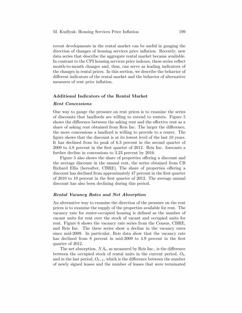
The Durbin Amendment and the resulting regulation were createdto resolve the long-time con�icts between card issuers and merchantsregarding payment card interchange fees. The interchange fee is theamount that a merchant has to pay the cardholder�s bank (the so-calledissuer) through the merchant acquiring bank (the so-called acquirer)when a card payment is processed. Merchants have criticized that cardnetworks (such as Visa and MasterCard) and their issuing banks haveused market power to set excessively high interchange fees, which driveup merchants�costs of accepting card payments. Card networks andissuers disagree, countering that interchange fees have been properly setto serve the needs of all parties in the card system, including fundingbetter consumer reward programs that could also bene�t merchants.
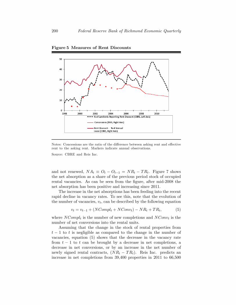
By capping debit card interchange fees, the regulation has gener-ated signi�cant impact on the U.S. payments industry since its imple-mentation. The most visible impact is the drop of multibillion-dollar
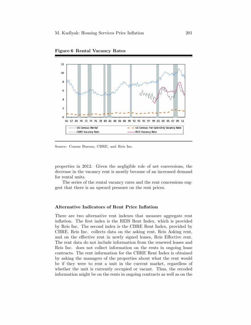
I thank Kartik Athreya, Borys Grochulski, Sam Marshall, and Ned Prescott forhelpful comments, and John Muth for excellent research assistance. The views ex-pressed herein are solely those of the author and do not necessarily re�ect the viewsof the Federal Reserve Bank of Richmond or the Federal Reserve System. E-mail:[email protected].
160 Federal Reserve Bank of Richmond Economic Quarterly
annual revenues for card issuers in terms of the interchange fees thatthey collect from merchants. Meanwhile, the regulation has yieldedother intended and unintended consequences. In this article, we reviewthe regulation�s impact from both positive and normative perspectives.We �rst look into the empirical evidence of the regulation�s �rst-yeare¤ects on di¤erent players in the debit card market, namely issuers,merchants, and consumers. We then provide a simple two-sided mar-ket model, based on the work of Rochet and Tirole (2011), to assessthe regulation�s implications on payments e¢ ciency. The model shedslight on important policy questions, for example, whether the debitcard market performs ine¢ ciently without regulation and whether theDurbin regulation can improve market outcome. Finally, we extendthe model to explain the regulation�s unintended consequence on small-ticket merchants and discuss an alternative regulatory approach.
The article is organized as follows. Section 1 provides the back-ground of payment card markets and the interchange fee regulation.Section 2 reviews the empirical evidence on the regulation�s impact ondi¤erent players in the debit card market. Section 3 lays out a simplemodel of the payment card market and discusses the regulation�s im-plication on payments e¢ ciency. We then extend the model to addressthe regulation�s unintended consequence on small-ticket merchants. Fi-nally, Section 4 provides concluding remarks.
1. INDUSTRY BACKGROUND
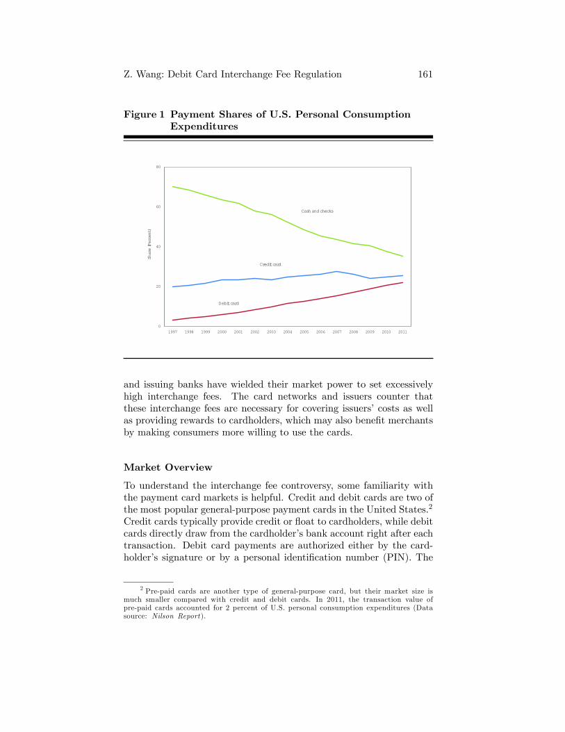
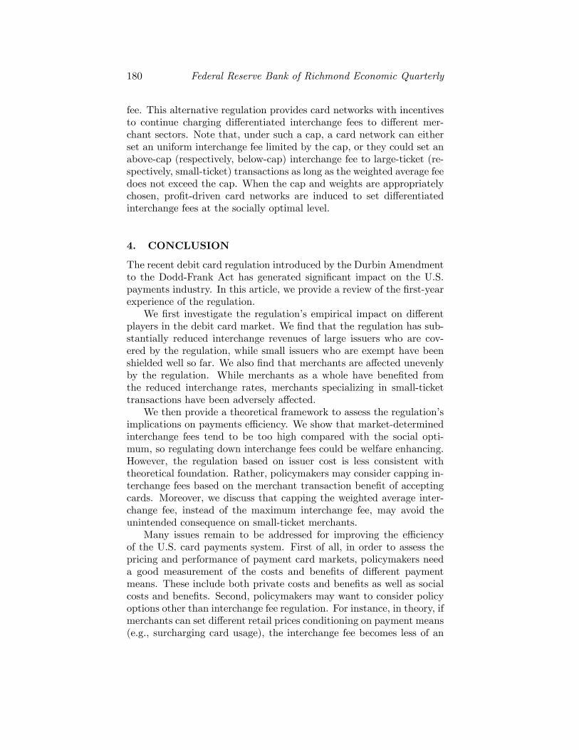
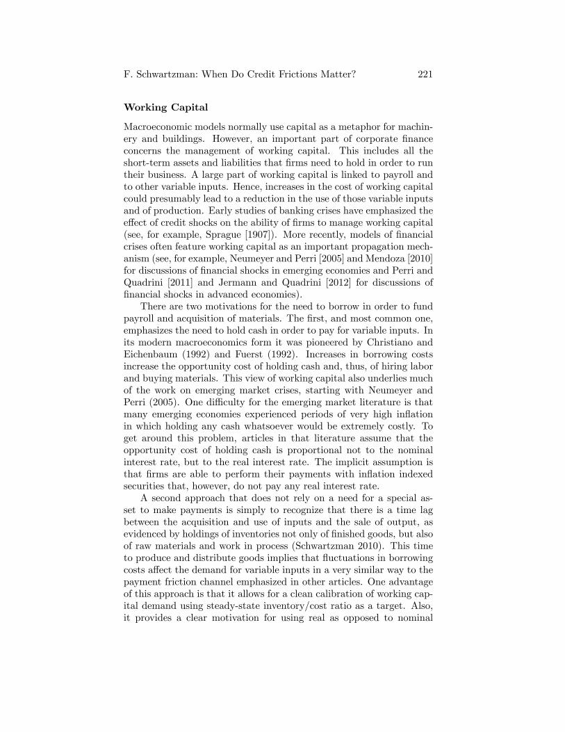
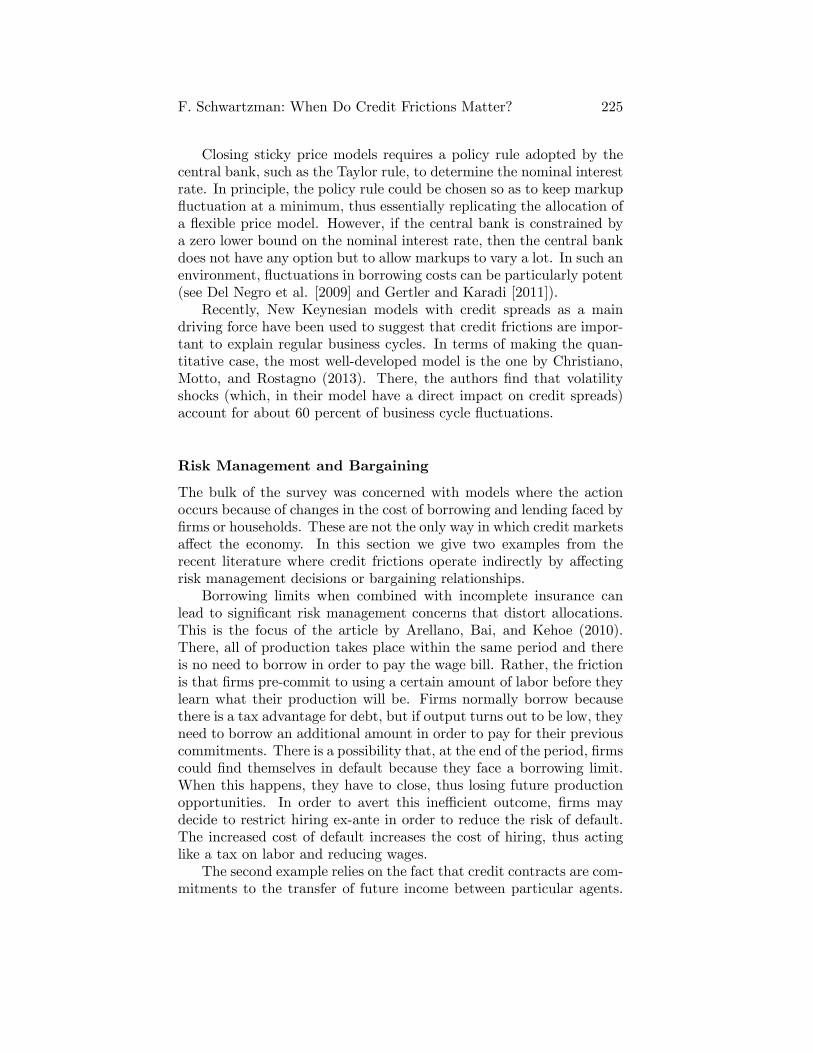
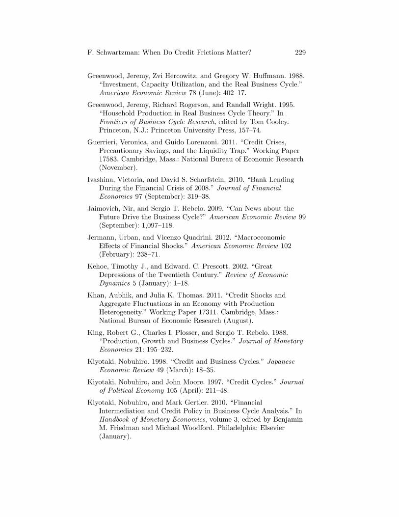
As payments migrate from paper to electronic forms, credit and debitcards have become an increasingly important part of the U.S. paymentssystem. Recent data show that the payment share of credit and debitcards in personal consumption expenditures rose from 23 percent in1997 to 48 percent in 2011, while the share of cash and checks droppedfrom 70 percent to 35 percent (Figure 1).1 In 2011, debit cards wereused in 49 billion transactions for a total value of $1.8 trillion, andcredit cards were used in 26 billion transactions for a total value of$2.1 trillion.
Along with this development has come controversy. Merchants arecritical of the fees that they pay to accept cards. These fees are oftenreferred to as the �merchant discounts,�which are composed mainlyof interchange fees paid by merchants to card issuing banks throughmerchant acquiring banks. Merchants believe that the card networks
1 The data are drawn from various issues of the Nilson Report. Payment shares notshown in Figure 1 include the automated clearing house and some other miscellaneoustypes.
Z. Wang: Debit Card Interchange Fee Regulation 161
Figure 1 Payment Shares of U.S. Personal ConsumptionExpenditures
and issuing banks have wielded their market power to set excessivelyhigh interchange fees. The card networks and issuers counter thatthese interchange fees are necessary for covering issuers�costs as wellas providing rewards to cardholders, which may also bene�t merchantsby making consumers more willing to use the cards.
Market Overview
To understand the interchange fee controversy, some familiarity withthe payment card markets is helpful. Credit and debit cards are two ofthe most popular general-purpose payment cards in the United States.2
Credit cards typically provide credit or �oat to cardholders, while debitcards directly draw from the cardholder�s bank account right after eachtransaction. Debit card payments are authorized either by the card-holder�s signature or by a personal identi�cation number (PIN). The
2 Pre-paid cards are another type of general-purpose card, but their market size ismuch smaller compared with credit and debit cards. In 2011, the transaction value ofpre-paid cards accounted for 2 percent of U.S. personal consumption expenditures (Datasource: Nilson Report ).
162 Federal Reserve Bank of Richmond Economic Quarterly
former is called signature debit and the latter is called PIN debit. Interms of transaction volume, signature debit accounts for 60 percent ofdebit transactions, while PIN debit accounts for 40 percent.
Visa and MasterCard are the two major credit card networks in theUnited States. They provide card services through member �nancialinstitutions and account for 85 percent of the U.S. consumer credit cardmarket.3 Visa and MasterCard are also the primary providers of debitcard services. The two networks split the signature debit market, withVisa holding 75 percent of the market share and MasterCard holding25 percent.4 In contrast, PIN debit transactions are routed over thePIN debit networks. Currently, there are 14 PIN debit networks inthe United States. Interlink, Star, Pulse, and NYCE are the top fournetworks, together holding 90 percent of the PIN debit market. Thelargest PIN network, Interlink, is operated by Visa.
Visa, MasterCard, and PIN debit networks are commonly referredto as four-party schemes because four parties are involved in each trans-action in addition to the network whose brand appears on the card.These parties include: (1) the cardholder who makes the purchase; (2)the merchant who makes the sale and accepts the card payment; (3)the �nancial institution that issues the card and makes the paymenton behalf of the cardholder (the so-called issuer); and (4) the �nancialinstitution that collects the payment on behalf of the merchant (theso-called acquirer).
In a four-party card scheme, interchange fees are collectively set bythe card network on behalf of their member issuers. For a simple ex-ample of how interchange functions, imagine a consumer making a $50purchase with a payment card. For that $50 item, the merchant wouldget approximately $49. The remaining $1, known as the merchant dis-count, gets divided up. About $0.80 would go to the card issuing bankas the interchange fee, and $0.20 would go to the merchant acquir-ing bank (the retailer�s account provider). Interchange fees serve asa key element of the four-party scheme business model and generatesigni�cant revenues for card issuers. In 2009, U.S. card issuers madeapproximately $48 billion revenue in interchange fees, with debit in-terchange revenues being $17 billion and credit interchange revenuesbeing $31 billion.5
3 American Express and Discover are the other two credit card networks holdingthe remaining market shares. They handle most card issuing and merchant acquiringby themselves, and are called �three-party� systems. For a �three-party� system, inter-change fees are internal transfers.
4 Discover has recently entered the signature debit market, but its market share issmall.
5 See Levitin (2010).
Z. Wang: Debit Card Interchange Fee Regulation 163
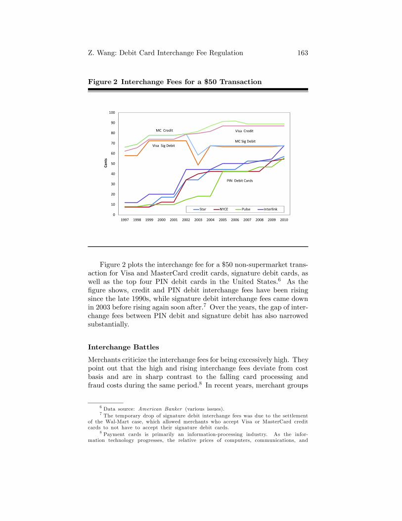
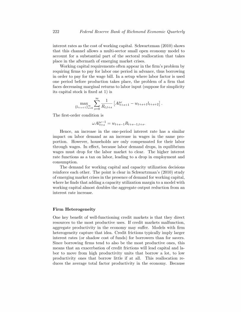
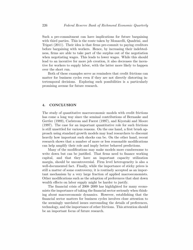
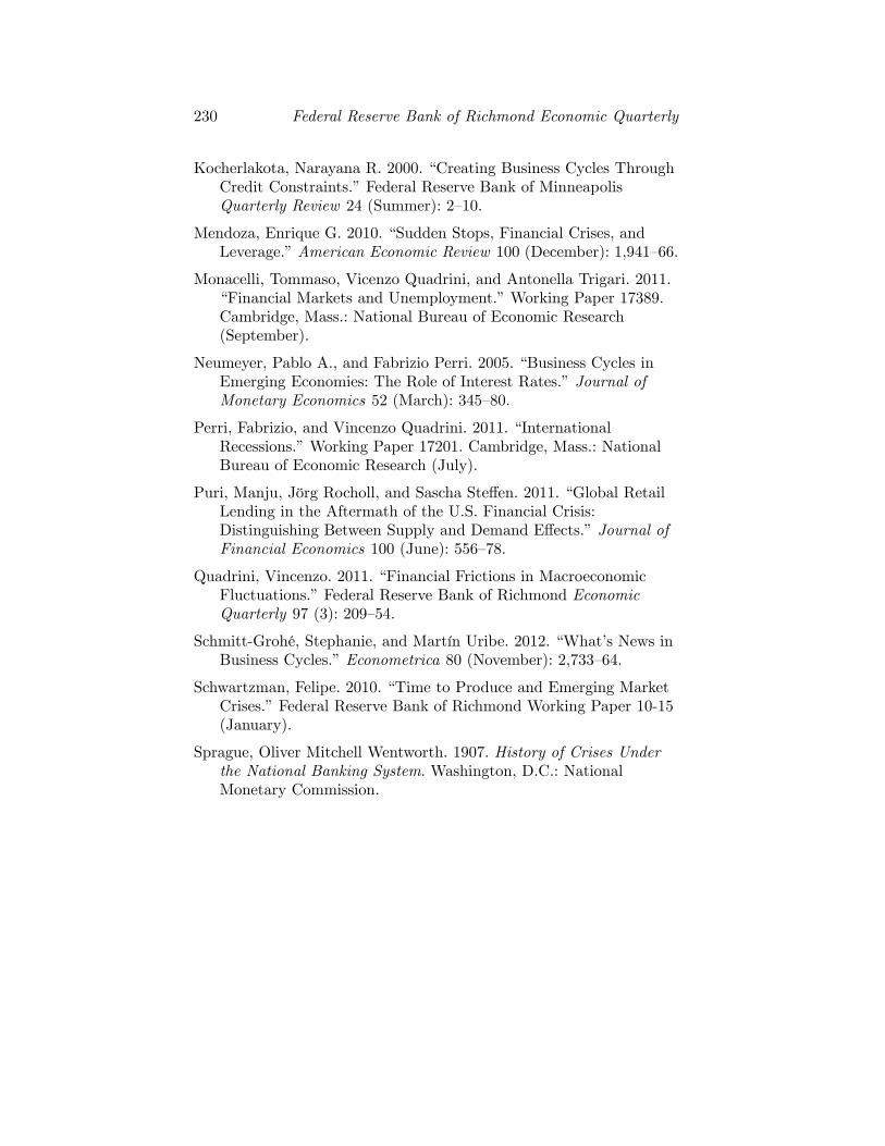
Figure 2 Interchange Fees for a $50 Transaction
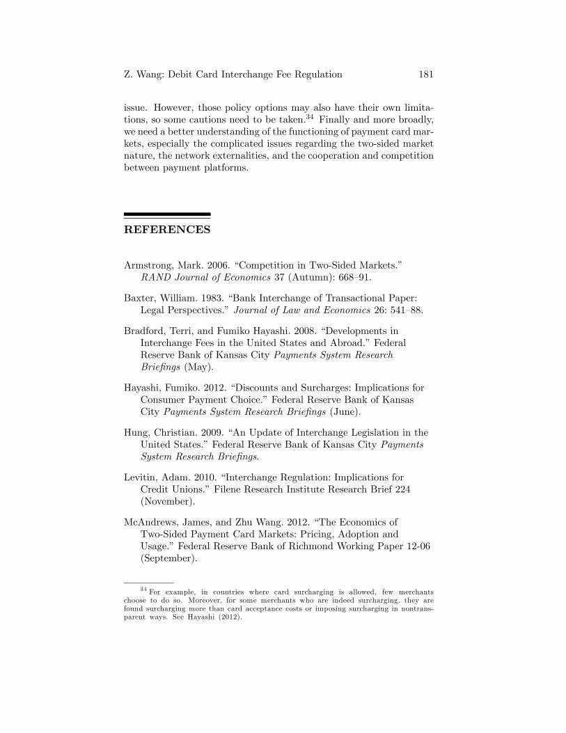
Figure 2 plots the interchange fee for a $50 non-supermarket trans-action for Visa and MasterCard credit cards, signature debit cards, aswell as the top four PIN debit cards in the United States.6 As the�gure shows, credit and PIN debit interchange fees have been risingsince the late 1990s, while signature debit interchange fees came downin 2003 before rising again soon after.7 Over the years, the gap of inter-change fees between PIN debit and signature debit has also narrowedsubstantially.
Interchange Battles
Merchants criticize the interchange fees for being excessively high. Theypoint out that the high and rising interchange fees deviate from costbasis and are in sharp contrast to the falling card processing andfraud costs during the same period.8 In recent years, merchant groups
6 Data source: American Banker (various issues).7 The temporary drop of signature debit interchange fees was due to the settlement
of the Wal-Mart case, which allowed merchants who accept Visa or MasterCard creditcards to not have to accept their signature debit cards.
8 Payment cards is primarily an information-processing industry. As the infor-mation technology progresses, the relative prices of computers, communications, and
164 Federal Reserve Bank of Richmond Economic Quarterly
launched a series of litigation against what they claim is anticompet-itive behavior by the card networks and their issuers. Some of thelawsuits have been aimed directly at interchange fees, including bothcredit and debit cards. For example, a group of class-action suits �ledby merchants against Visa and MasterCard in 2005 alleged that thenetworks violated antitrust laws by engaging in price �xing. As a re-sult, Visa and MasterCard recently agreed to a $7.25 billion settlementwith U.S. retailers, which could be the largest antitrust settlement inU.S. history.9 Other merchant lawsuits have focused not on interchangefees per se, but on alleged anticompetitive practices. A prime exampleis the lawsuit �led by Wal-Mart and other merchants in 1997 againstthe networks�honor-all-cards rule, which required a merchant accept-ing a network�s credit cards to also accept its signature debit cards.The Wal-Mart case was settled in 2003. As a result, Visa and Master-Card agreed to unbundle credit cards and signature debit cards, andalso temporarily lowered their interchange fees on signature debit cards(Figure 2).
The interchange fee controversy has also attracted great attentionfrom policymakers, who are concerned that interchange fees in�ate thecost of card acceptance without leading to proven e¢ ciency.10 In thetwo years leading up to the passage of the Durbin Amendment, threeseparate bills restricting interchange fees were introduced in Congress:a House version of the Credit Card Fair Fee Act of 2009, a Senateversion of the same act, and the Credit Card Interchange Fees Act of2009.11 Before any of these bills could be brought to a vote, the Dodd-Frank Act was passed and signed into law in July 2010. A provisionof the Dodd-Frank Act, known as the Durbin Amendment, mandatesa regulation aimed at debit card interchange fees and increasing com-petition in the payment processing industry.
software have been declining rapidly, which should have driven down the card processingcosts. Meanwhile, industry statistics show that card fraud rates also have been decliningsteadily. For the U.S. credit card industry as a whole, the net fraud losses as a percentof total transaction volume has dropped from roughly 16 basis points in 1992 to about7 basis points in 2009. Data source: Nilson Report (various issues).
9 Visa, MasterCard, and their major issuers reached the settlement agreement withmerchants in July 2012. The settlement is currently pending �nal court approval.
10 Worldwide, more than 20 countries and areas have started regulating or inves-tigating interchange fees. Primary examples include Australia, Canada, the EuropeanUnion, France, Spain, and the United Kingdom (Bradford and Hayashi 2008).
11 None of the bills called for direct regulation of interchange fees, and all threeapplied to interchange fees for both credit and debit cards (Hung 2009).
Z. Wang: Debit Card Interchange Fee Regulation 165
Durbin Amendment and Regulation
The Durbin Amendment of the Dodd-Frank Act directs the FederalReserve Board to regulate debit card interchange fees �reasonable andproportional to the cost incurred by the issuer with respect to thetransaction.�The Federal Reserve Board subsequently issued the �nalrule on debit cards in July 2011, e¤ective on October 1, 2011.
The Federal Reserve Board ruling establishes a cap on the debit in-terchange fees that �nancial institutions with more than $10 billion inassets can charge to merchants through merchant acquirers. The per-missible fees were set based on the Federal Reserve Board�s evaluationof issuers�costs associated with debit card processing, clearance, andsettlement. The resulting interchange cap is composed of the following:a base fee of 21 cents per transaction to cover the issuer�s processingcosts, a �ve basis point adjustment to cover potential fraud losses, andan additional 1 cent per transaction to cover fraud prevention costs ifthe issuer is eligible. This cap applies to both signature and PIN debittransactions.
In addition, the regulation sets rules that prohibit certain restraintsimposed by card networks on merchants. First, networks can no longerprohibit merchants from o¤ering customers discounts for using debitcards versus credit cards. This gives merchants a way to steer con-sumers toward using less expensive payment means.12 Second, issuersmust put at least two una¢ liated networks on each debit card and areprohibited from inhibiting a merchant�s ability to direct the routing ofdebit card transactions. This gives merchants more freedom for rout-ing debit transactions through less costly networks. Third, networkscan no longer forbid merchants from setting minimum values for creditcard payments. Going forward, merchants are allowed to establish suchminimum values as long as the minimum does not exceed $10.
2. EMPIRICAL IMPACT
A direct impact of the debit card regulation is the redistribution of in-terchange revenues from issuers to merchants. According to a FederalReserve study, the average debit card transaction in 2009 was approx-imately $40. Post regulation, the maximum interchange fee applicableto a typical debit card transaction is capped at 24 cents (21 cents+ ($40 � .05%) + 1 cent), which is about half of its pre-regulation
12 Since the passage of the Cash Discount Act in 1981, merchants have been allowedto o¤er their customers discounts for paying with cash or checks. However, the cardnetworks have continued to prohibit merchants from o¤ering customers discounts forusing one type of card rather than another.
166 Federal Reserve Bank of Richmond Economic Quarterly
industry average level. As a result, issuers were expected to lose multi-billion dollar annual revenues in terms of the interchange fees that theycollect from merchants. In this section, we look into the empirical ev-idence of the regulation�s �rst-year e¤ects on di¤erent players in thedebit card market.
Impact on Issuers
The regulation reduces debit card interchange fees by about half andalso introduces more competition by abolishing certain network restric-tions. As a result, issuers face a big drop in their interchange revenues.Meanwhile, the regulation allows small issuers to be exempt from theinterchange fee cap� those with less than $10 billion in assets.13
To assess the regulation�s impact on covered and exempt issuers,we conduct a study on a subsample of card issuers, which includesall the commercial banks that report their interchange revenues in thequarterly Call Report. Our sample includes 7,049 commercial banksbetween the �rst quarter of 2009 and the third quarter of 2012. Amongthose, we identify 102 covered issuers and 6,969 exempt issuers. Thestatus of exemption is based on whether the bank asset value exceedsthe $10 billion threshold as of prior year end.14
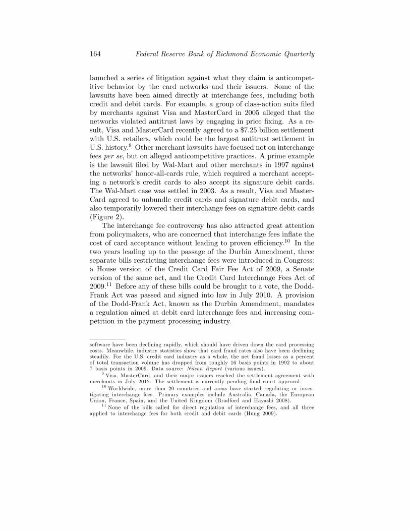
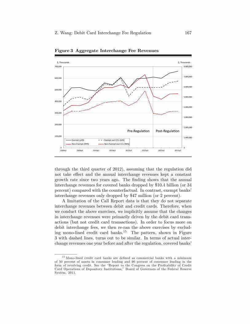
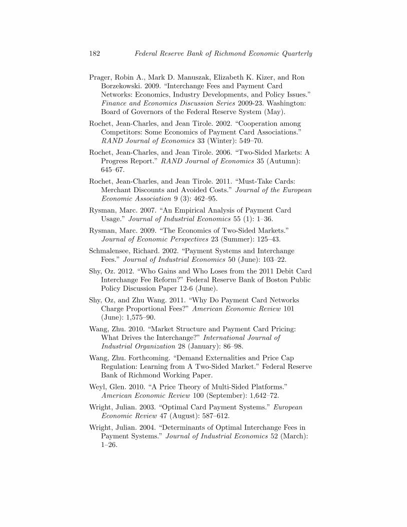
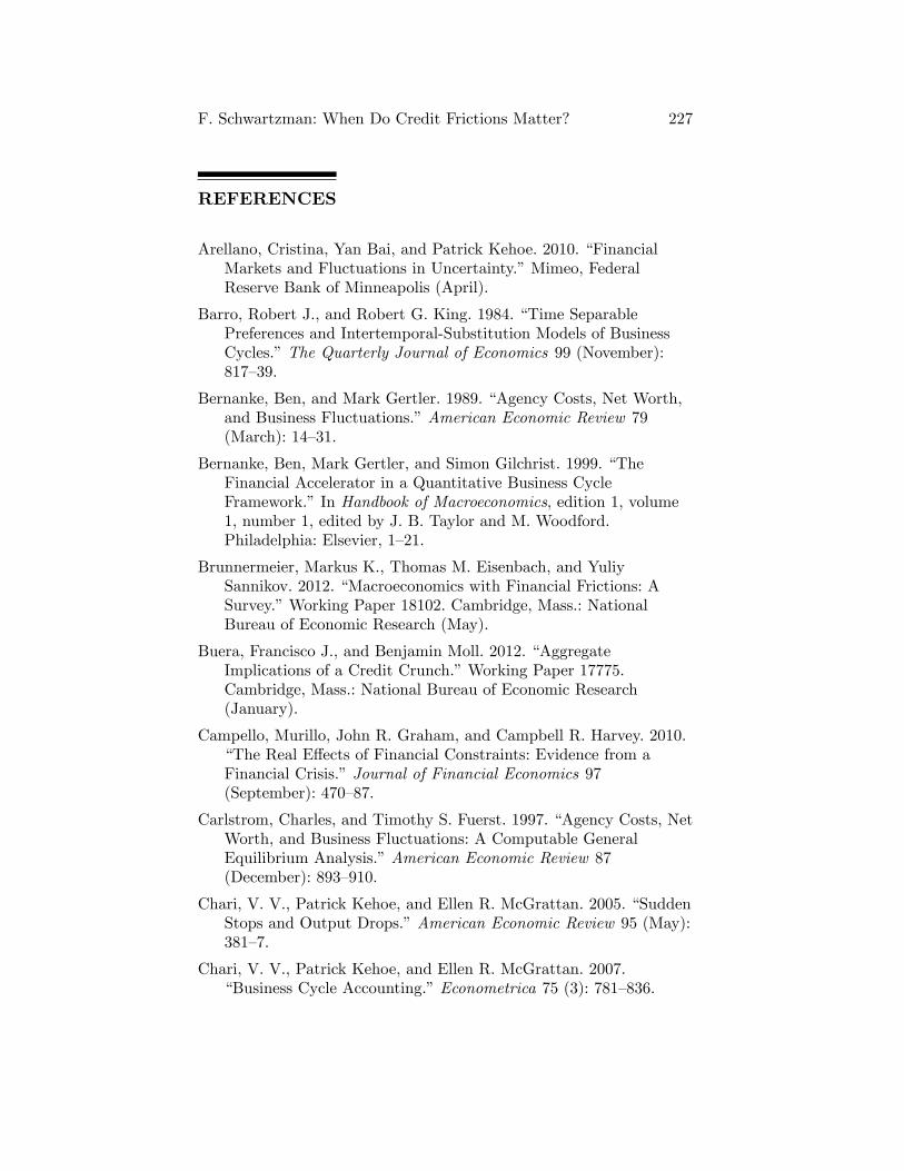
We �rst compare the interchange revenues of all covered and ex-empt banks right before and right after the regulation, as shown inFigure 3 with solid lines. Covered banks had a substantial loss of in-terchange revenues during the period. Between the third quarter andfourth quarter of 2011 (i.e., the immediate quarter before and after theregulation took e¤ect), covered banks� interchange revenues droppedby $2.1 billion (or 29 percent), equivalent to an $8.5 billion drop an-nually. In contrast, exempt banks�quarterly interchange revenues didnot fall during the same period, instead rising by $11.8 million (or 2percent).
We also compare the interchange revenues one year before and oneyear after the regulation to control for potential seasonality. The resultis similar: Covered banks� annual interchange revenues dropped by$5.4 billion (or 21 percent), while exempt banks�annual interchangerevenues increased by $198 million (or 9 percent).
For an alternative check, we construct counterfactual interchangerevenues for one year after the regulation (the fourth quarter of 2011
13 This exemption is applied at the holding company level, to ensure that largeissuers cannot evade the regulations by establishing subsidiaries under the size limit.
14 Note that a bank�s exemption status may change as its asset size changes, sothe sum of non-exempt banks and exempt banks may exceed the total number of banksin the sample.
Z. Wang: Debit Card Interchange Fee Regulation 167
Figure 3 Aggregate Interchange Fee Revenues
through the third quarter of 2012), assuming that the regulation didnot take e¤ect and the annual interchange revenues kept a constantgrowth rate since two years ago. The �nding shows that the annualinterchange revenues for covered banks dropped by $10.4 billion (or 34percent) compared with the counterfactual. In contrast, exempt banks�interchange revenues only dropped by $47 million (or 2 percent).
A limitation of the Call Report data is that they do not separateinterchange revenues between debit and credit cards. Therefore, whenwe conduct the above exercises, we implicitly assume that the changesin interchange revenues were primarily driven by the debit card trans-actions (but not credit card transactions). In order to focus more ondebit interchange fees, we then re-ran the above exercises by exclud-ing mono-lined credit card banks.15 The pattern, shown in Figure3 with dashed lines, turns out to be similar. In terms of actual inter-change revenues one year before and after the regulation, covered banks�
15 Mono-lined credit card banks are de�ned as commercial banks with a minimumof 50 percent of assets in consumer lending and 90 percent of consumer lending in theform of revolving credit. See the �Report to the Congress on the Pro�tability of CreditCard Operations of Depository Institutions,� Board of Governors of the Federal ReserveSystem, 2011.
168 Federal Reserve Bank of Richmond Economic Quarterly
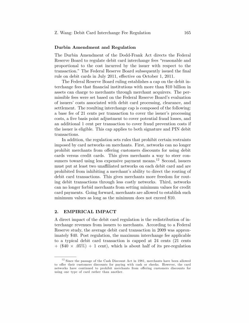
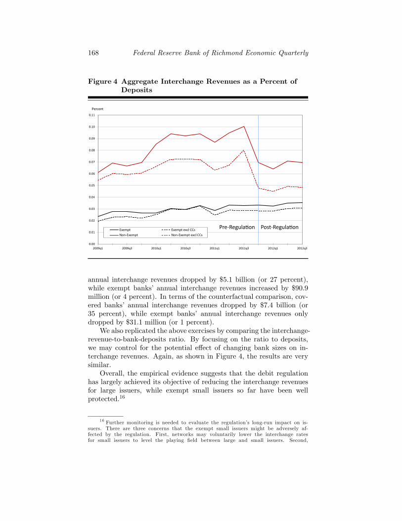
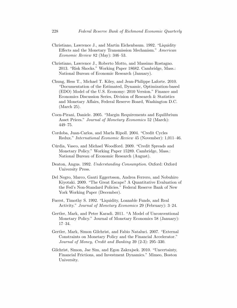
Figure 4 Aggregate Interchange Revenues as a Percent ofDeposits
annual interchange revenues dropped by $5.1 billion (or 27 percent),while exempt banks� annual interchange revenues increased by $90.9million (or 4 percent). In terms of the counterfactual comparison, cov-ered banks� annual interchange revenues dropped by $7.4 billion (or35 percent), while exempt banks� annual interchange revenues onlydropped by $31.1 million (or 1 percent).
We also replicated the above exercises by comparing the interchange-revenue-to-bank-deposits ratio. By focusing on the ratio to deposits,we may control for the potential e¤ect of changing bank sizes on in-terchange revenues. Again, as shown in Figure 4, the results are verysimilar.
Overall, the empirical evidence suggests that the debit regulationhas largely achieved its objective of reducing the interchange revenuesfor large issuers, while exempt small issuers so far have been wellprotected.16
16 Further monitoring is needed to evaluate the regulation�s long-run impact on is-suers. There are three concerns that the exempt small issuers might be adversely af-fected by the regulation. First, networks may voluntarily lower the interchange ratesfor small issuers to level the playing �eld between large and small issuers. Second,
Z. Wang: Debit Card Interchange Fee Regulation 169
Impact on Merchants
Merchants as a whole have greatly bene�ted from the reduced inter-change fees under the regulation. Presumably, the loss of issuers� in-terchange revenues would be the gain of the merchants. However, thedistribution of the gain appears uneven among merchants. In fact, theregulation has yielded an unintended consequence: Interchange feesrose for small-ticket merchants.
Prior to the regulation, Visa, MasterCard, and most PIN networkso¤ered discounted debit interchange fees to small-ticket transactions asa way to encourage card acceptance by merchants specializing in thosetransactions. For example, Visa and MasterCard used to set the small-ticket signature debit interchange rate at 1.55 percent of the transactionvalue plus 4 cents for sales of $15 and below. As a result, a debit cardwould only charge a 7 cents interchange fee for a $2 sale or 11 cents fora $5 sale. However, in response to the regulation, card networks elimi-nated the small-ticket discounts, and all transactions (except those oncards issued by exempt issuers) have to pay the maximum cap amountset by the regulation (i.e., 21 cents plus 0.05 percent of the transactionvalue).17 For merchants selling small-ticket items, this means that thecost of accepting the same debit card doubled or even tripled after theregulation.
The rising interchange fee on small-ticket sales could a¤ect a largenumber of transactions. According to the 2010 Federal Reserve Pay-ments Study, in 2009 debit cards were used for 4.9 billion transactionsbelow $5, and 10.8 billion transactions between $5�$15. The formeraccounts for 8.3 percent of all payment card transactions (includingcredit, debit, and prepaid cards), and the latter accounts for 18.3 per-cent. Since merchants may have di¤erent compositions of transactionsizes, they could be a¤ected di¤erently by the changes of interchangefees.18 However, merchants who specialize in small-ticket transactionswould be most adversely a¤ected.19
merchants may o¤er preferential treatment to cards issued by large issuers that carrylower interchange rates. Third, the regulation requires each debit card be connectedto at least two una¢ liated networks and merchants have the freedom to choose thelower-cost routing. This provision took e¤ect after April 2012 and small issuers are notexempt from it.
17 E.g., in the case of signature debit, any sales below $11 now face a higher in-terchange rate.
18 Shy (2012) used the data from the Boston Fed�s 2010 and 2011 Diary of Con-sumer Payment Choice to identify the types of merchants who are likely to pay higherand lower interchange fees under the debit regulation.
19 E.g., Visa classi�es merchant sectors specializing in small-ticket sales, which in-clude local commuter transport, taxicabs and limousine, fast food restaurants, co¤eeshops, parking lots and garages, motion picture theaters, video rental stores, cashless
170 Federal Reserve Bank of Richmond Economic Quarterly
In response, many small-ticket merchants have tried to o¤set theirhigher rates by raising prices, encouraging customers to pay with al-ternative payment means, or dropping card payments altogether.20 Inthe meantime, a lawsuit was �led in November 2011 in federal court bythree of the retail industry�s largest trade associations and two retailcompanies against the Federal Reserve�s debit interchange regulation.The lawsuit alleges that the Fed has set the interchange cap too highby including costs that were barred by the law, and �forcing small busi-nesses to pay three times as much to the big banks on small purchaseswas clearly not the intent of the law and is further evidence that theFed got it wrong.�21
The unintended consequence on small-ticket merchants calls fora further examination on the regulation, which we will provide inSection 3.
Impact on Consumers
The regulation�s impact on consumers is less clear. On the one hand,merchants argue that with a lower interchange fee, they would be ableto o¤er lower retail prices to consumers. On the other hand, issuersargue that they will have to reduce card rewards and raise bankingservice fees to consumers in order to make up for the lost interchangerevenues.
At this point, little empirical evidence has been reported on thechange of merchant prices due to the debit interchange regulation. Af-ter all, even if the reduced interchange fees have resulted in lower retailprices, the magnitude would be quite small so it is not easy to mea-sure. Meanwhile, several studies report that consumers now face higherbanking and card service fees. A recent Pulse debit issuer study showsthat 50 percent of regulated debit card issuers with a reward programended their programs in 2011, and another 18 percent planned to doso in 2012.22 The Bankrate�s 2012 Checking Survey shows that the av-erage monthly fee of noninterest checking accounts rose by 25 percent
vending machines and kiosks, bus lines, tolls and bridge fees, news dealers, laundries,dry cleaners, quick copy, car wash and service stations, etc.
20 See �Debit-Fee Cap Has Nasty Side E¤ect,� Wall Street Journal, December 8,2011.
21 Source: �Merchants� Lawsuit Says Fed Failed to Follow Law on Swipe FeeReform,� Business Wire, November 22, 2011.
22 The 2012 Debit Issuer Study, commissioned by Pulse, is based on research with57 banks and credit unions that collectively represent approximately 87 million debitcards and 47,000 ATMs. Research was conducted in April and May of 2012, and thedata provided by issuers is for 2011. The sample is nationally representative, with issuerssegmented into �regulated� (� $10 billion in assets) and �exempt� (< $10 billion inassets) to report on the impact of the interchange provision of Regulation II.
Z. Wang: Debit Card Interchange Fee Regulation 171
compared with last year, and the minimum balance for free-checkingservices rose by 23 percent.23 According to the report, the rising bankfees are largely due to banks�response to recent regulations includingthe debit interchange cap. In addition, several major banks includ-ing Bank of America, Wells Fargo, and Chase attempted to chargea monthly debit card fee to their customers in response to the inter-change regulation, but they eventually backed down due to customeroutrage.24
3. THEORETICAL CONSIDERATIONS
The debit card regulation was created to reduce the interchange fee bycapping the fee at the card issuers�marginal cost. To understand thewelfare implications of the regulation, we turn to a theoretical analysisin this section.
First, we lay out a simple model based on the work of Rochet andTirole (2011). The model conceptualizes payment cards as a two-sidedmarket, that is, two end-user groups (i.e., merchants and consumers)who jointly use the card services.25 The interchange fee serves as atransfer between merchants and consumers to balance their joint de-mand for using cards. Under the assumption of homogenous merchants,the model shows that (1) market-determined interchange fees tend toexceed the socially optimal level, so reducing interchange fees mayimprove the payments e¢ ciency; (2) however, capping interchange feesbased on issuers�marginal cost does not necessarily restore the socialoptimum; and (3) the theory suggests an interchange fee regulationbased on the merchant transaction bene�t of accepting cards.
While the simple two-sided market model sheds light on key policyissues related to the interchange fee regulation, it does not address theregulation�s unintended consequence on small-ticket merchants. To �llthe gap, we then introduce an extension of the model by consideringcard demand externalities across heterogenous merchant sectors, basedon the work of Wang (forthcoming). The �ndings suggest that an
23 Bankrate surveyed banks in the top 25 U.S. cities to �nd the average fees as-sociated with checking accounts in their annual Checking Account Survey, which wasconducted in July and August 2012.
24 Source: �Banks Adding Debit Card Fees,� The New York Times, September 29,2011.
25 In recent years, a sizeable body of literature, called �two-sided market the-ory,� has been developed to evaluate payment card market competition and pricing is-sues. For instance, Baxter (1983), Rochet and Tirole (2002, 2006, 2011), Schmalensee(2002), Wright (2003, 2004, 2012), Armstrong (2006), Rysman (2007, 2009), Prageret al. (2009), Wang (2010, forthcoming), Weyl (2010), Shy and Wang (2011), andMcAndrews and Wang (2012).
172 Federal Reserve Bank of Richmond Economic Quarterly
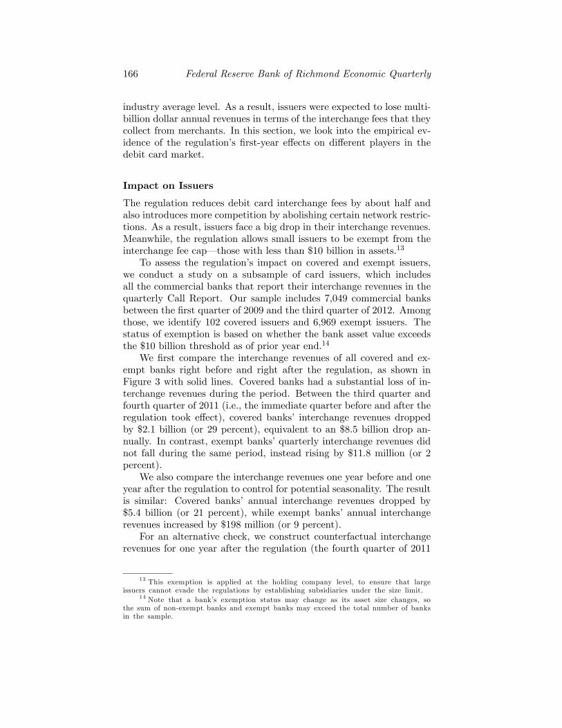
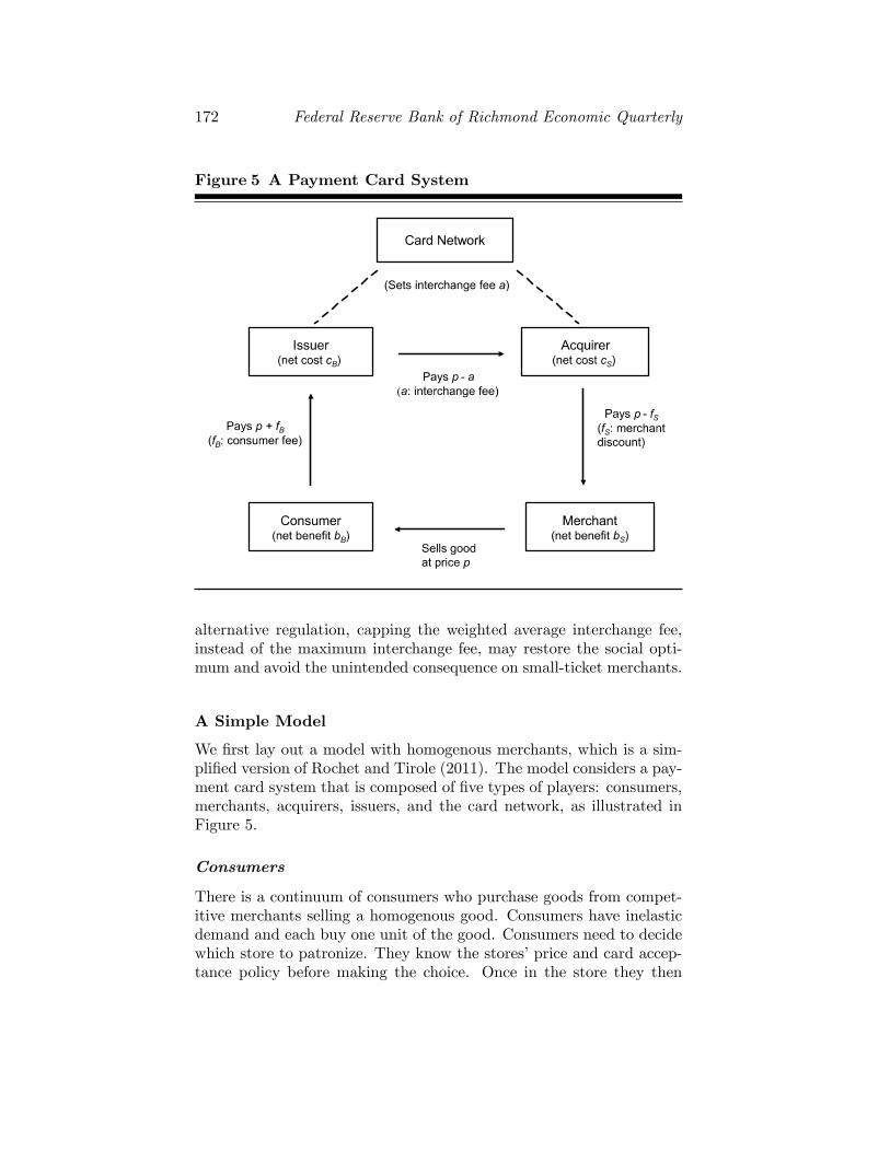
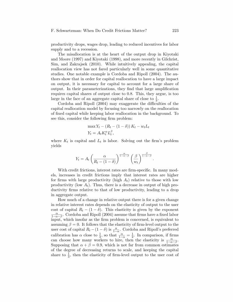
Figure 5 A Payment Card System
alternative regulation, capping the weighted average interchange fee,instead of the maximum interchange fee, may restore the social opti-mum and avoid the unintended consequence on small-ticket merchants.
A Simple Model
We �rst lay out a model with homogenous merchants, which is a sim-pli�ed version of Rochet and Tirole (2011). The model considers a pay-ment card system that is composed of �ve types of players: consumers,merchants, acquirers, issuers, and the card network, as illustrated inFigure 5.
Consumers
There is a continuum of consumers who purchase goods from compet-itive merchants selling a homogenous good. Consumers have inelasticdemand and each buy one unit of the good. Consumers need to decidewhich store to patronize. They know the stores�price and card accep-tance policy before making the choice. Once in the store they then
Z. Wang: Debit Card Interchange Fee Regulation 173
select a payment method (a card or an alternative payment methodsuch as cash), provided that the retailer indeed o¤ers a choice amongpayment means. We assume price coherence such that retailers �ndit too costly to charge di¤erent prices for purchases made by di¤er-ent payment means.26 Whenever a transaction between a consumer(buyer) and a retailer (seller) is settled by card, the buyer pays a feefB to her card issuing bank (issuer) and the seller pays a merchantdiscount fS to her merchant acquiring bank (acquirer). We allow fBto be negative, in which case the cardholder receives a card reward.There are no annual fees and all consumers have a card.
The consumer�s convenience bene�t of paying by card relative to us-ing cash is a random variable bB drawn from a cumulative distributionfunction H on the support [bB; bB], which has a monotonic increasinghazard rate.27 Cardholders are assumed to only observe the realizationof bB once in the store.28 Because the net bene�t of paying by cardis equal to the di¤erence bB � fB, a card payment is optimal for theconsumer whenever bB � fB. The proportion of card payments at astore that accepts cards is denoted D(fB):
D(fB) = Pr(bB � fB) = 1�H(fB): (1)
Let v(fB) denote the average net cardholder bene�t per card pay-ment:
v(fB) = E[bB � fBjbB � fB]
=
R bBfB(bB � fB)dH(bB)1�H(fB)
> 0: (2)
The monotonic hazard rate of H implies that v(fB) decreases in fB.
26 Price coherence is the key feature that de�nes a two-sided market. Rochet andTirole (2006) show that the two-sided market pricing structure (e.g., interchange fees)would become irrelevant without the price coherence condition. In reality, price coher-ence may result either from network rules or state regulation, or from high transactioncosts for merchants to price discriminate based on payment means. In the United States,while merchants are allowed to o¤er their customers discounts for paying with cash orchecks, few merchants choose to do so. On the other hand, card network rules and somestate laws explicitly prohibit surcharging on payment cards.
27 The hazard rate is assumed increasing to guarantee concavity of the optimizationproblem.
28 This is a standard assumption introduced by Wright (2004) and used in the sub-sequent literature, which simpli�es the analysis of retailers� acceptance of cards withoutchanging the equilibrium outcome. Alternatively, Rochet and Tirole (2002) assume card-holders di¤er systematically in the bene�t that they derive from card payments. How-ever, as shown in Rochet and Tirole (2011), these two alternative assumptions deliverbroadly convergent results.
174 Federal Reserve Bank of Richmond Economic Quarterly
Merchants
Merchants derive the convenience bene�t bS of accepting payment cards(relative to handling cash). By accepting cards under the price coher-ence assumption, a merchant is able to o¤er each of its card-holdingcustomers an additional expected surplus of D(fB)v(fB), but faces anadditional expected net cost of D(fB)(fS� bS) per cardholder. Denotec as the cost of the good. Competitive merchants then set a retail priceequal to marginal cost, namely
p = c+D(fB)(fS � bS) (3)
if they accept cards, or p = c if they reject cards. Consumers choose thestores that accept cards if and only if their increased surplusD(fB)v(fB)exceeds the price increase D(fB)(fS�bS). Therefore, all merchants ac-cept cards if and only if
fS � bS + v(fB): (4)
Rochet and Tirole (2011) show that (4) also holds for a variety ofother merchant competition setups, including monopoly and Hotelling-Lerner-Salop di¤erentiated products competition with any number ofretailers. Wright (2010) shows the same condition holds for Cournotcompetition.
Acquirers
We assume acquirers incur per-transaction cost cS and are perfectlycompetitive. Thus, given an interchange fee a, they charge a merchantdiscount fS such that
fS = a+ cS : (5)
Because acquirers are competitive, they play no role in our analysisexcept passing through the interchange charge to merchants.
Issuers
Issuers are assumed to have market power.29 We consider a sym-metric oligopolistic equilibrium at which all issuers charge the same
29 This is a standard assumption in the literature. As pointed out in Rochet andTirole (2002), the issuer market power may be due to marketing strategies, search costs,reputation, or the nature of the card. Note that were the issuing side perfectly com-petitive, issuers and card networks would have no preference over the interchange fee,and so the latter would be indeterminate.
Z. Wang: Debit Card Interchange Fee Regulation 175
consumer fee fB, which can be negative if the cardholder receives areward. Issuers incur a per-transaction cost cB and receive an inter-change payment of a for a card transaction. At equilibrium, the netper-transaction cost for issuers is cB � a. For simplicity, we considerthat issuers set a constant markup '.30 Hence, the consumer fee fB isdetermined as
fB = '+ cB � a: (6)
Network
We consider a monopoly network, which sets the interchange fee a tomaximize the total pro�t of issuers from card transactions, namely,
� = 'D(fB) = '[1�H(fB)] :Alternatively, we could consider a regulator who instead sets the inter-change fee to maximize social welfare or user surplus.
Timing
The timing of events is as follows.
1. The card network (or the regulator) sets the interchange fee a.
2. Issuers and acquirers set fees fB and fS . Merchants then decidewhether to accept cards and set retail prices.
3. Consumers observe the retail prices and whether cards are ac-cepted, and choose a store. Once in the store, the consumerreceives her draw of bB and decides which payment method touse.
Model Characterization
We �rst consider the market equilibrium under a monopoly network.Given the model setup, the network solves the following problem:
maxa
'[1�H(fB)] (7)
s:t: fB = '+ cB � a; (8)
30 This is a simplifying assumption, and the �ndings of the model hold if we insteadconsider an endogenous issuer markup. See Wang (forthcoming).
176 Federal Reserve Bank of Richmond Economic Quarterly
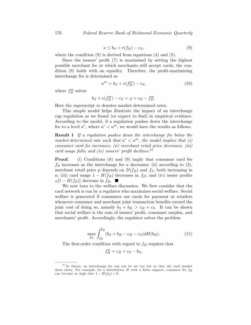
a � bS + v(fB)� cS ; (9)
where the condition (9) is derived from equations (4) and (5).Since the issuers� pro�t (7) is maximized by setting the highest
possible merchant fee at which merchants still accept cards, the con-dition (9) holds with an equality. Therefore, the pro�t-maximizinginterchange fee is determined as
am = bS + v(fmB )� cS ; (10)
where fmB solves
bS + v(fmB )� cS = '+ cB � fmB :
Here the superscript m denotes market-determined rates.This simple model helps illustrate the impact of an interchange
cap regulation as we found (or expect to �nd) in empirical evidence.According to the model, if a regulation pushes down the interchangefee to a level ar, where ar < am, we would have the results as follows.
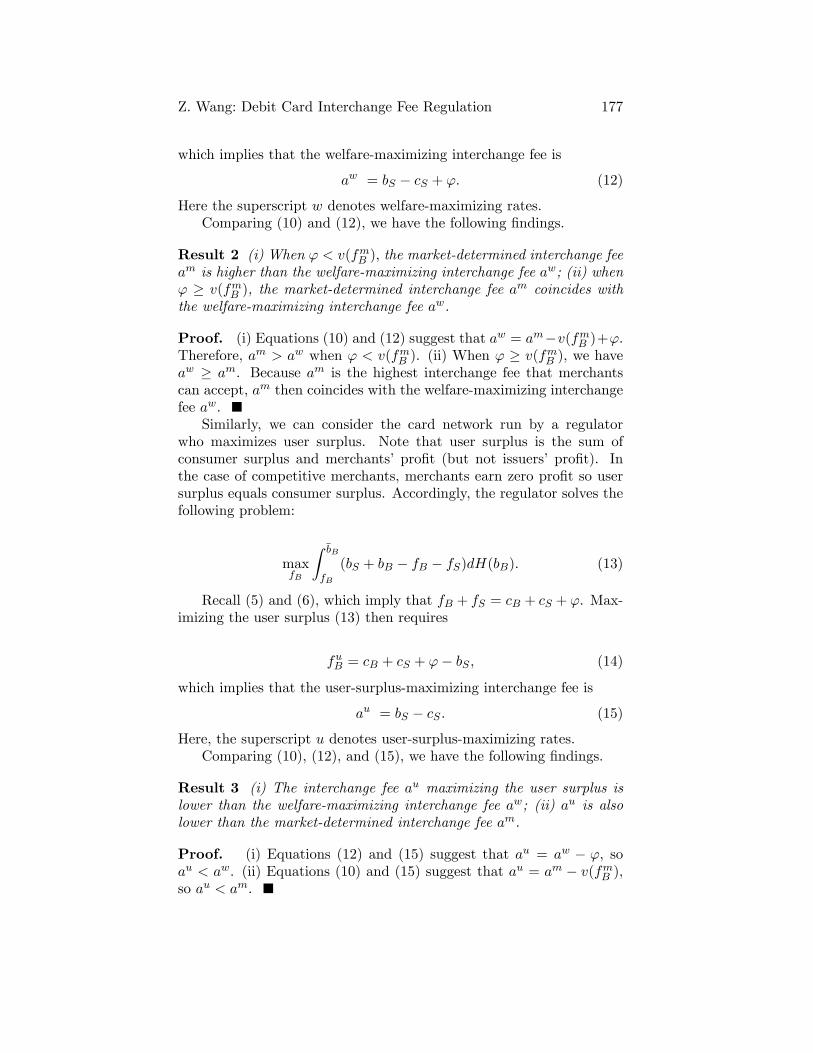
Result 1 If a regulation pushes down the interchange fee below themarket-determined rate such that ar < am, the model implies that (i)consumer card fee increases; (ii) merchant retail price decreases; (iii)card usage falls; and (iv) issuers�pro�t declines.31
Proof. (i) Conditions (8) and (9) imply that consumer card feefB increases as the interchange fee a decreases; (ii) according to (3),merchant retail price p depends on D(fB) and fS , both increasing ina; (iii) card usage 1 � H(fB) decreases in fB; and (iv) issuer pro�ts'[1�H(fB)] decrease in fB.
We now turn to the welfare discussion. We �rst consider that thecard network is run by a regulator who maximizes social welfare. Socialwelfare is generated if consumers use cards for payment at retailerswhenever consumer and merchant joint transaction bene�ts exceed thejoint cost of doing so, namely bS + bB > cB + cS . It can be shownthat social welfare is the sum of issuers�pro�t, consumer surplus, andmerchants�pro�t. Accordingly, the regulator solves the problem
maxfB
Z bB
fB
(bS + bB � cB � cS)dH(bB): (11)
The �rst-order condition with regard to fB requires that
fwB = cB + cS � bS ;
31 In theory, an interchange fee cap can be set too low so that the card marketshuts down. For example, for a distribution H with a �nite support, consumer fee fBcan become so high that 1�H(fB) = 0:
Z. Wang: Debit Card Interchange Fee Regulation 177
which implies that the welfare-maximizing interchange fee is
aw = bS � cS + ': (12)
Here the superscript w denotes welfare-maximizing rates.Comparing (10) and (12), we have the following �ndings.
Result 2 (i) When ' < v(fmB ); the market-determined interchange feeam is higher than the welfare-maximizing interchange fee aw; (ii) when' � v(fmB ), the market-determined interchange fee a
m coincides withthe welfare-maximizing interchange fee aw.
Proof. (i) Equations (10) and (12) suggest that aw = am�v(fmB )+'.Therefore, am > aw when ' < v(fmB ). (ii) When ' � v(fmB ), we haveaw � am. Because am is the highest interchange fee that merchantscan accept, am then coincides with the welfare-maximizing interchangefee aw.
Similarly, we can consider the card network run by a regulatorwho maximizes user surplus. Note that user surplus is the sum ofconsumer surplus and merchants� pro�t (but not issuers� pro�t). Inthe case of competitive merchants, merchants earn zero pro�t so usersurplus equals consumer surplus. Accordingly, the regulator solves thefollowing problem:
maxfB
Z bB
fB
(bS + bB � fB � fS)dH(bB): (13)
Recall (5) and (6), which imply that fB + fS = cB + cS + '. Max-imizing the user surplus (13) then requires
fuB = cB + cS + '� bS ; (14)
which implies that the user-surplus-maximizing interchange fee is
au = bS � cS : (15)
Here, the superscript u denotes user-surplus-maximizing rates.Comparing (10), (12), and (15), we have the following �ndings.
Result 3 (i) The interchange fee au maximizing the user surplus islower than the welfare-maximizing interchange fee aw; (ii) au is alsolower than the market-determined interchange fee am.
Proof. (i) Equations (12) and (15) suggest that au = aw � ', soau < aw. (ii) Equations (10) and (15) suggest that au = am � v(fmB ),so au < am.
178 Federal Reserve Bank of Richmond Economic Quarterly
Results 2 and 3 show that the market-determined interchange feetends to be too high, based on the criterion of either social welfaremaximization or user surplus maximization. The reason is that underprice coherence, merchants internalize consumers�expected card usagebene�ts when they decide whether to accept cards and set retail prices.This allows the card network to charge too high an interchange fee andtoo low a consumer fee. As a result, cards get used even when consumerand merchant joint card usage costs exceed their joint transaction ben-e�ts. Therefore, regulating down the interchange fee may potentiallyimprove payments e¢ ciency.
However, (12) and (15) also clarify that the socially optimal inter-change fee is not determined by the issuer cost, cB, but rather by themerchant transaction bene�t of accepting cards, bS . Particularly, (15)suggests that a regulator may consider setting the merchant discountfS = bS , at which the resulting interchange fee maximizes the usersurplus. This is the criterion proposed by Rochet and Tirole (2011),which they call the �merchant avoided-cost test.�32
Small-Ticket E�ect
Our analysis so far does not explain the regulation�s unintended conse-quence on small-ticket merchants. This is largely because we have onlyassumed homogenous merchants in the model. However, even if in amodel with multiple (heterogenous) merchant sectors, as long as thosemerchant sectors are independent from one another in terms of card ac-ceptance and usage, it is still a puzzle to think why card networks wouldabandon the interchange di¤erentiation in response to a cap regulation.In other words, if it was pro�table for a card network to charge a lowerfee to small-ticket merchants in the absence of regulation, why wouldthe card network want to change the practice because of a non-bindingcap? To address this issue, Wang (forthcoming) extends the modelof Rochet and Tirole (2011) by considering card demand externalitiesacross merchant sectors.
In the setup of Wang (forthcoming), there are multiple merchantsectors (e.g., large-ticket merchants and small-ticket merchants). Dif-ferent merchant sectors are charged di¤erent interchange fees due totheir (observable) heterogenous bene�ts of card acceptance and usage.In addition, consumers�bene�ts of using cards in a merchant sector are
32 Focusing on user surplus is legitimate if card issuer pro�ts are not consideredor weighed much less by competition authorities. The criterion proposed by Rochetand Tirole (2011) is adopted by the European Commission and renamed the �merchantindi¤erence test,� while some other countries, including the United States and Australia,adopt the issuer cost-based cap regulation.
Z. Wang: Debit Card Interchange Fee Regulation 179
positively a¤ected by their card usage in other sectors, which is calledthe �ubiquity externalities.�33 Based on this setup, Wang (forthcoming)again �nds that market-determined interchange fees tend to exceed thesocially optimal level. The reason is similar to before: Under price co-herence, consumers are provided with excessive incentives to use cards.In addition, Wang (forthcoming) o¤ers the following new �ndings.
Result 4 (i) Card demand externalities across merchant sectors ex-plain why card networks eliminate the interchange fee discount to small-ticket merchants in response to the interchange cap regulation; (ii) thesocial planner who maximizes social welfare would set a discounted in-terchange fee for small-ticket merchants; (iii) capping the weighted av-erage interchange fee, instead of the maximum interchange fee, mayrestore the social optimum and avoid the unintended consequence onsmall-ticket merchants.
Wang (forthcoming) o¤ers a formal derivation of the above results.Here we provide an intuitive discussion. First, the �ubiquity�external-ities may explain card networks�pricing response to the cap regulation:Before the regulation, card networks o¤er a discounted interchange fee(i.e., a subsidy) to small-ticket merchants because their card acceptanceboosts consumers�card usage for large-ticket purchases from which cardissuers can collect higher interchange fees. After the regulation, how-ever, the interchange fees on large-ticket purchases are capped. Asa result, card issuers pro�t less from this kind of externality so cardnetworks discontinued the discount.
Second, despite privately determined interchange fees tending to ex-ceed the socially optimal level, the social planner who maximizes socialwelfare would behave similar to the private network by setting di¤er-entiated interchange fees, i.e., charging a high interchange fee to large-ticket merchants but a low interchange fee to small-ticket merchants.Essentially, both the social planner and the private network treat thesmall-ticket transactions as a loss leader. By subsidizing small-tickettransactions, they internalize the positive externalities of card usagebetween the small-ticket and large-ticket sectors.
Third, it is possible to design a cap regulation that may restore thesocial optimum and avoid the unintended consequence on small-ticketmerchants. Conceptually, this can be done by imposing a cap on theweighted average interchange fee instead of the maximum interchange
33 Ubiquity has always been a top selling point for brand cards. This is clearlyshown in card networks� advertising campaigns, such as Visa�s �It is everywhere youwant to be,� and MasterCard�s �There are some things money can�t buy. For everythingelse, there�s MasterCard.�
180 Federal Reserve Bank of Richmond Economic Quarterly
fee. This alternative regulation provides card networks with incentivesto continue charging di¤erentiated interchange fees to di¤erent mer-chant sectors. Note that, under such a cap, a card network can eitherset an uniform interchange fee limited by the cap, or they could set anabove-cap (respectively, below-cap) interchange fee to large-ticket (re-spectively, small-ticket) transactions as long as the weighted average feedoes not exceed the cap. When the cap and weights are appropriatelychosen, pro�t-driven card networks are induced to set di¤erentiatedinterchange fees at the socially optimal level.
4. CONCLUSION
The recent debit card regulation introduced by the Durbin Amendmentto the Dodd-Frank Act has generated signi�cant impact on the U.S.payments industry. In this article, we provide a review of the �rst-yearexperience of the regulation.
We �rst investigate the regulation�s empirical impact on di¤erentplayers in the debit card market. We �nd that the regulation has sub-stantially reduced interchange revenues of large issuers who are cov-ered by the regulation, while small issuers who are exempt have beenshielded well so far. We also �nd that merchants are a¤ected unevenlyby the regulation. While merchants as a whole have bene�ted fromthe reduced interchange rates, merchants specializing in small-tickettransactions have been adversely a¤ected.
We then provide a theoretical framework to assess the regulation�simplications on payments e¢ ciency. We show that market-determinedinterchange fees tend to be too high compared with the social opti-mum, so regulating down interchange fees could be welfare enhancing.However, the regulation based on issuer cost is less consistent withtheoretical foundation. Rather, policymakers may consider capping in-terchange fees based on the merchant transaction bene�t of acceptingcards. Moreover, we discuss that capping the weighted average inter-change fee, instead of the maximum interchange fee, may avoid theunintended consequence on small-ticket merchants.
Many issues remain to be addressed for improving the e¢ ciencyof the U.S. card payments system. First of all, in order to assess thepricing and performance of payment card markets, policymakers needa good measurement of the costs and bene�ts of di¤erent paymentmeans. These include both private costs and bene�ts as well as socialcosts and bene�ts. Second, policymakers may want to consider policyoptions other than interchange fee regulation. For instance, in theory, ifmerchants can set di¤erent retail prices conditioning on payment means(e.g., surcharging card usage), the interchange fee becomes less of an
Z. Wang: Debit Card Interchange Fee Regulation 181
issue. However, those policy options may also have their own limita-tions, so some cautions need to be taken.34 Finally and more broadly,we need a better understanding of the functioning of payment card mar-kets, especially the complicated issues regarding the two-sided marketnature, the network externalities, and the cooperation and competitionbetween payment platforms.
REFERENCES
Armstrong, Mark. 2006. �Competition in Two-Sided Markets.�RAND Journal of Economics 37 (Autumn): 668�91.
Baxter, William. 1983. �Bank Interchange of Transactional Paper:Legal Perspectives.�Journal of Law and Economics 26: 541�88.
Bradford, Terri, and Fumiko Hayashi. 2008. �Developments inInterchange Fees in the United States and Abroad.�FederalReserve Bank of Kansas City Payments System ResearchBrie�ngs (May).
Hayashi, Fumiko. 2012. �Discounts and Surcharges: Implications forConsumer Payment Choice.�Federal Reserve Bank of KansasCity Payments System Research Brie�ngs (June).
Hung, Christian. 2009. �An Update of Interchange Legislation in theUnited States.�Federal Reserve Bank of Kansas City PaymentsSystem Research Brie�ngs.
Levitin, Adam. 2010. �Interchange Regulation: Implications forCredit Unions.�Filene Research Institute Research Brief 224(November).
McAndrews, James, and Zhu Wang. 2012. �The Economics ofTwo-Sided Payment Card Markets: Pricing, Adoption andUsage.�Federal Reserve Bank of Richmond Working Paper 12-06(September).
34 For example, in countries where card surcharging is allowed, few merchantschoose to do so. Moreover, for some merchants who are indeed surcharging, they arefound surcharging more than card acceptance costs or imposing surcharging in nontrans-parent ways. See Hayashi (2012).
182 Federal Reserve Bank of Richmond Economic Quarterly
Prager, Robin A., Mark D. Manuszak, Elizabeth K. Kizer, and RonBorzekowski. 2009. �Interchange Fees and Payment CardNetworks: Economics, Industry Developments, and Policy Issues.�Finance and Economics Discussion Series 2009-23. Washington:Board of Governors of the Federal Reserve System (May).
Rochet, Jean-Charles, and Jean Tirole. 2002. �Cooperation amongCompetitors: Some Economics of Payment Card Associations.�RAND Journal of Economics 33 (Winter): 549�70.
Rochet, Jean-Charles, and Jean Tirole. 2006. �Two-Sided Markets: AProgress Report.�RAND Journal of Economics 35 (Autumn):645�67.
Rochet, Jean-Charles, and Jean Tirole. 2011. �Must-Take Cards:Merchant Discounts and Avoided Costs.�Journal of the EuropeanEconomic Association 9 (3): 462�95.
Rysman, Marc. 2007. �An Empirical Analysis of Payment CardUsage.�Journal of Industrial Economics 55 (1): 1�36.
Rysman, Marc. 2009. �The Economics of Two-Sided Markets.�Journal of Economic Perspectives 23 (Summer): 125�43.
Schmalensee, Richard. 2002. �Payment Systems and InterchangeFees.�Journal of Industrial Economics 50 (June): 103�22.
Shy, Oz. 2012. �Who Gains and Who Loses from the 2011 Debit CardInterchange Fee Reform?�Federal Reserve Bank of Boston PublicPolicy Discussion Paper 12-6 (June).
Shy, Oz, and Zhu Wang. 2011. �Why Do Payment Card NetworksCharge Proportional Fees?�American Economic Review 101(June): 1,575�90.
Wang, Zhu. 2010. �Market Structure and Payment Card Pricing:What Drives the Interchange?�International Journal ofIndustrial Organization 28 (January): 86�98.
Wang, Zhu. Forthcoming. �Demand Externalities and Price CapRegulation: Learning from A Two-Sided Market.�Federal ReserveBank of Richmond Working Paper.
Weyl, Glen. 2010. �A Price Theory of Multi-Sided Platforms.�American Economic Review 100 (September): 1,642�72.
Wright, Julian. 2004. �Determinants of Optimal Interchange Fees inPayment Systems.�Journal of Industrial Economics 52 (March):1�26.
Economic Quarterly� Volume 98, Number 3� Third Quarter 2012� Pages 185�207
Housing Services PriceIn ation
Marianna Kudlyak
The cost of housing services constitutes more than 30 percent ofthe cost of the consumer basket used to measure the consumerprice index (hereafter, CPI), a major indicator of in�ation in
the consumer prices produced by the Bureau of Labor Statistics (BLS).Thus, understanding housing services price in�ation is important forunderstanding the aggregate �uctuations of prices in the economy.
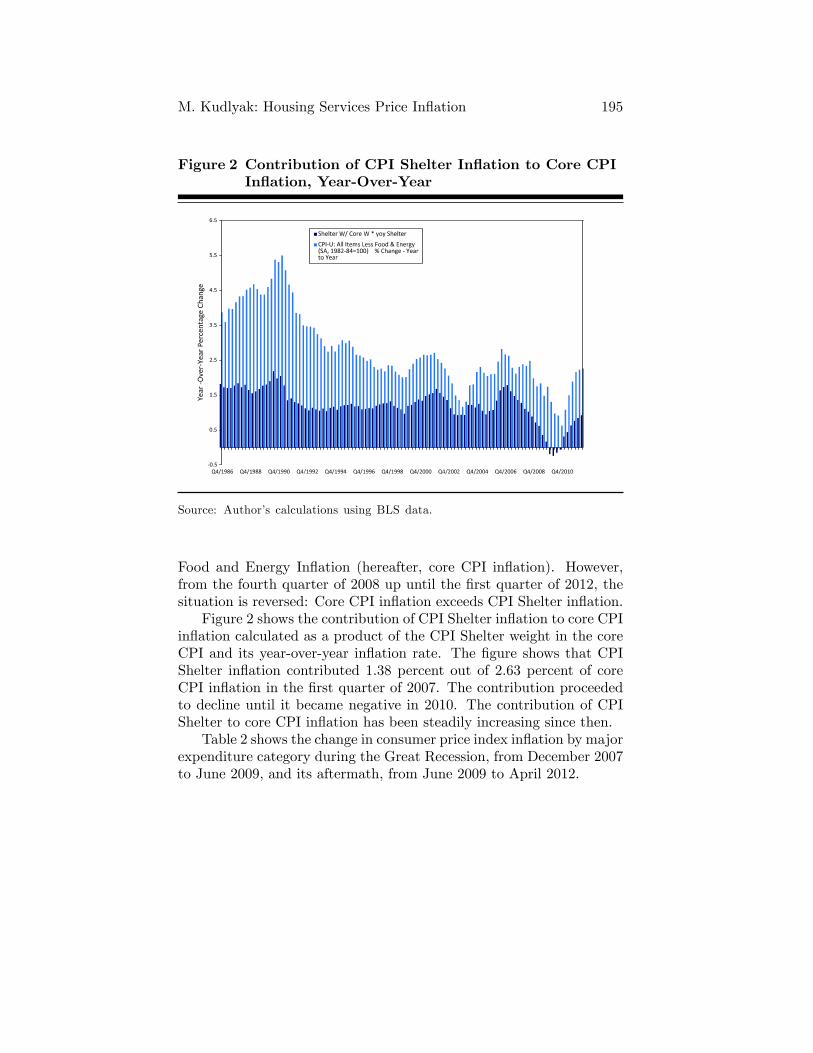
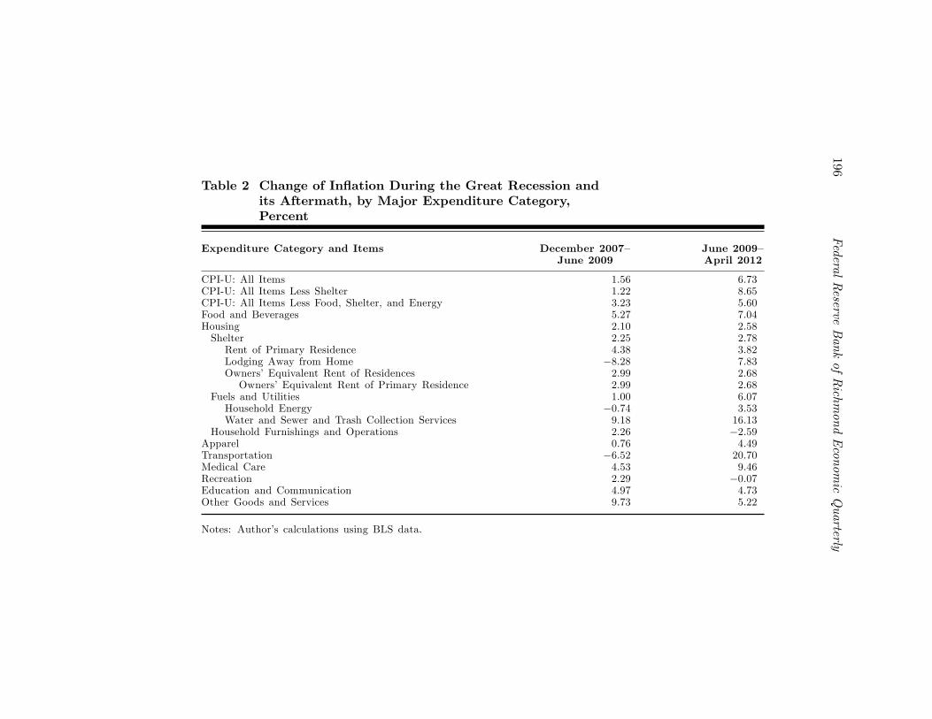
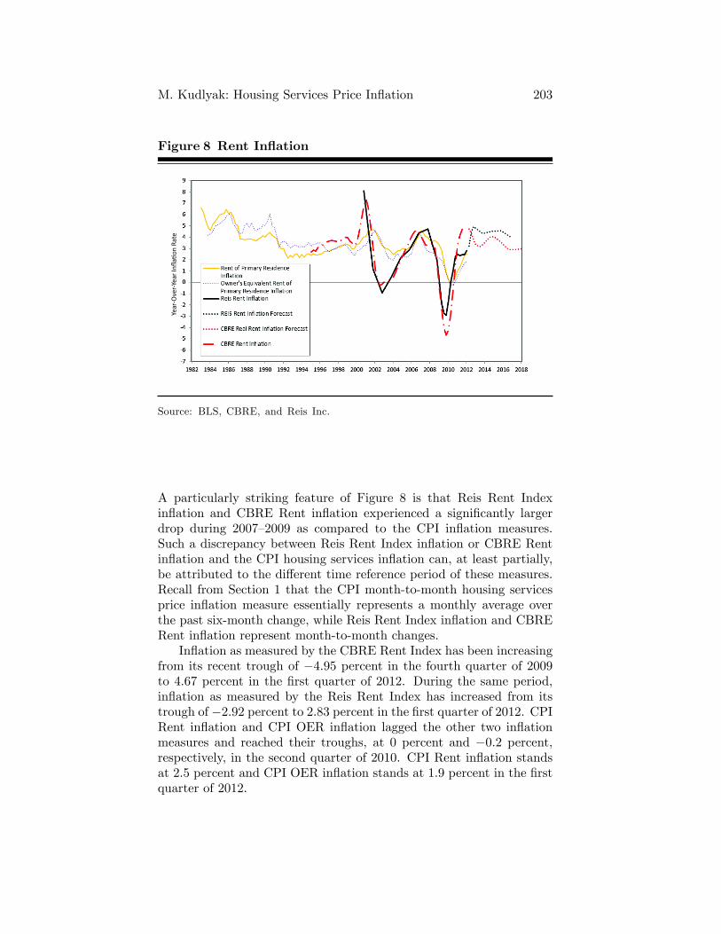
In this article, we provide an explanation of how in�ation of theprice of housing services is measured by the BLS and describe alter-native approaches. We then describe the contribution of in�ation ofthe price of housing services to in�ation in the CPI during the GreatRecession and its aftermath.1 Finally, we examine new data seriesthat provide additional information about the rental market for hous-ing services and use this information to evaluate the direction of thepressure on housing services price in�ation (hereafter, housing servicesin�ation).
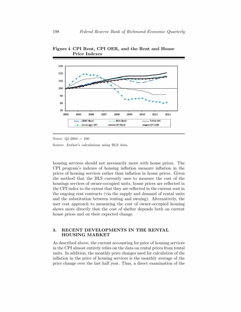
Between 2005 and 2007, housing services in�ation, as measured bythe CPI, was rising, while house price in�ation exhibited a steep decline.Such periods, i.e., when the CPI measure of housing services in�ationdiverges particularly far from house price in�ation, often reignite thedebate about whether the CPI adequately re�ects the cost of housingservices.
This debate fails to recognize that the CPI program measures theprice of the services provided by housing and not the price of the as-set (i.e., house) itself. If the household buys the housing services in
The author is grateful to Andreas Hornstein, Robert Hetzel, Zhu Wang, andJonathan Tompkins for their generous comments and suggestions. Steven Sabol pro-vided excellent research assistance. The views expressed here are those of the authorand do not necessarily re�ect those of the Federal Reserve Bank of Richmond orthe Federal Reserve System. E-mail: [email protected].
1 In the analysis, we use data up through the second quarter of 2012.
186 Federal Reserve Bank of Richmond Economic Quarterly
the market, i.e., rents an apartment, then the rental price is the priceof the services. If the household owns the housing unit that provideshousing services, then the price of the �ow of housing services that thehousehold receives must be imputed because the price is not observed.Given that a majority of U.S. households own their housing, the impu-tation procedure is one of the main issues associated with calculatingthe CPI. The measure of the hypothetical rent paid by homeowners isthe major component of the CPI and is called the owner�s equivalentrent (OER).
This article argues that the changes in the price of housing servicesshould not necessarily move with the changes of house prices. In par-ticular, currently, the BLS calculates the owner�s equivalent rent usinga rental-equivalence approach, in which only data on rental prices arecollected. Under this approach, the house prices are re�ected in theCPI to the extent that they are re�ected in the current rent in theongoing rent contracts. An alternative imputation mechanism for theowner�s equivalent rent is the user cost approach. The user cost ap-proach is arguably more attractive conceptually because it explicitlytreats a house as an asset. The user cost approach shows directly thatthe cost of housing services depends not only on the contemporaneoushouse prices but also on their expected change. Despite being con-ceptually more attractive, the user cost approach has proven hard toimplement in practice.
Currently, the monthly CPI housing services in�ation is measuredby a repeat-rent index, which represents the monthly average of thechange in the rental price of rental units over the last six months.Recently, new data on the rental housing market, which re�ect month-to-month changes, have become available. Examining the series thatdescribe month-to-month changes can help gauge the direction of changesof the CPI housing services in�ation index in upcoming months. Weexamine the behavior of the new series on residential rents, rental va-cancies, and rent concessions. The developments in the rental housingmarket suggest that since 2010 there has been increasing upward pres-sure on housing services in�ation.
The remainder of the article is organized as follows. The nextsection describes the measurement of housing services price in�ation.Section 2 summarizes the recent behavior of housing services price in-�ation as measured by the BLS. Section 3 examines new additionalseries that describe the rental housing market. Section 4 concludes.
M. Kudlyak: Housing Services Price In ation 187
1. ACCOUNTING FOR HOUSING SERVICESPRICE INFLATION
Current Accounting for Housing in the CPI
The CPI is a cost of living index, that is, the cost of generating a certainlevel of consumption for a certain time period, usually a month. Theconstruction of the CPI views housing units as capital goods ratherthan as consumption items. The relevant consumption item for theCPI is shelter� the service that the housing unit provides. The CPIShelter constitutes the major part of the CPI.
The CPI Shelter represents a weighted average of the four com-ponent indexes: (1) rent of primary residence (CPI Rent), (2) owners�equivalent rent of primary residence (CPI OER), (3) lodging away fromhome, and (4) tenants�and household insurance. Residential rents andOER data are collected from the CPI Housing Survey. The other twocomponents, lodging away from home and tenants�and household in-surance, are obtained from the CPI Commodities and Services Survey.
The CPI program calculates the price of the housing services of theowner-occupied housing using the rental equivalence approach. Un-der this approach, the cost of the shelter services provided by owner-occupied housing is the implicit rent (i.e., the amount the owner wouldpay for rent or would earn from renting his home in a competitive mar-ket) that is imputed from the actual rental prices collected from renters.The BLS employs the re-weighting method to the rental equivalenceapproach of calculating the hypothetical rents paid by homeowners.Under this method, the owners�equivalent of rent is calculated by re-weighting the rent sample to represent owner-occupied units.
Essentially, the CPI Rent and the CPI OER are the repeat-rentindexes, the information for which is collected from rental units. Theidea behind the index is to obtain the price change between period tand period t + 1 for the same rental unit, and then aggregate theseprice changes. The rent information in period t and in t+1 is collectedfrom the same unit to ensure that recoded change in rent is because ofin�ation rather than the quality di¤erence between t and t + 1. Thequality di¤erence is an issue because it is conceivable that in the casewith housing, rental or owner-occupied, there are large unmeasureddi¤erences in the quality. Each rental unit is surveyed every six months.Thus, the CPI Rent and the CPI OER de�ne the month-to-monthchange in the price of housing services as the average monthly pricechange over the last half year. The Appendix contains details on (1)
188 Federal Reserve Bank of Richmond Economic Quarterly
how the data on rental prices are collected, and (2) how the data areused to construct the CPI Rent and the CPI OER.2
For cost e¢ ciency, each rental unit is surveyed every six months.The CPI Rent is a weighted average of the change in the same-unitrents where the weights re�ect the quality distribution of rental units.The CPI OER is a weighted average of the same rent changes (minusthe cost of utilities if they are included in the rent) where the weightsre�ect the OER characteristics in the sample. The CPI Rent and theCPI OER de�ne the month-to-month change in the price of housingservices as the average monthly price change over the last half year.
A few additional notes are in order. First, for segments that containlargely owner-occupied housing, the CPI program selects rental unitsfrom the nearby segments. Second, for the vacant rental units, the es-timated current rent is its previous rent times the average rent changeof newly occupied units. Third, some rental units represent only rentalunits (for example, rental units under rent control), while other rentalunits represent only owner-occupied units. The CPI program�s han-dling of the rental units under rent control and the di¤erences betweeneconomic and pure rent contribute to the di¤erences between OER andRent indexes.
As described above, the existing CPI approach to accounting forowner-occupied housing services simply re-weights the rent sample torepresent owner-occupied units. Prior to 1999, the BLS employed thematching method to the rental equivalence approach (Diewert andNakamura 2009). Under this method, information is collected fromboth renter and owner samples. Then, the owner�s unit is matchedwith a renter�s unit with similar characteristics (i.e., location, struc-ture type, age, number of rooms, type of air conditioning, and otherattributes). The change in implicit rent is derived from the change inthe pure rents of its matched set of renters. However, this method re-quires large cost associated with collecting data from both renters andowners and is no longer used.
We can identify two main problems associated with the currentaccounting for housing in the CPI. First, most rental contracts arelong-term, and rents are sticky in the ongoing contracts. There is alsoconsiderable evidence that the rents are sticky not only within the con-tracts but also within the entire tenure of a renter with a particular
2 In this section we largely follow the BLS description of the measurement of CPIin�ation (see Bureau of Labor Statistics [2007, 2009)]). See Diewert and Nakamura(2009); Diewert, Nakamura, and Nakamura (2009); and Crone, Nakamura, and Voith(2010) for a description of the current measurement approach. Wolman (2011) providesan alternative in�ation measure that uses a di¤erent aggregation procedure for the ex-isting CPI components.
M. Kudlyak: Housing Services Price In ation 189
landlord (for example, Genesove [2003]). Thus, houses cannot likely berented at the same price as the rental units in ongoing rent contracts.Consequently, the rents in newly signed leases, which re�ect the con-temporaneous house prices and rental vacancies, might better re�ectthe implicit rent of owner-occupied housing. Second, rental housingmight not be that close a substitute for owner-occupied housing.3 Analternative approach to calculating the rental price of owner-occupiedhousing, the user cost approach, explicitly recognizes that a house isa capital good and addresses some of these concerns. We discuss theuser cost approach next.
User Cost Approach
The user cost approach to owner-occupied housing treats the servicesprovided by owner-occupied dwellings di¤erently from the services pro-vided by rental dwellings. The user cost of housing services can bethought of as a cost to a household of purchasing a house at the begin-ning of the period, living in it during the period, and then selling it atthe end of the period at the prevailing market price.
Kudlyak (2009) uses a similar approach to measure the �rm�s laborcost. Since employment relationships often last for more than one pe-riod, wage usually does not represent the period�s labor cost but ratherit is an installment payment on an employment contract. Kudlyakempirically constructs the user cost of labor, which is the di¤erencebetween the present discounted value of wages to be paid to a workerhired in the current period and the expected present discounted valueof wages to be paid to a worker hired the next period. Importantly,she �nds that the user cost of labor is much more procyclical than theaverage wage or the wage of newly hired workers in the economy be-cause of the e¤ect the economic conditions at the time of hiring haveon future wages within the employment relationship.
To introduce the user cost, let V vt denote the purchase price of av-year durable in year t, uvt denote the end-of-period value of the periodt services provided by this durable, Ovt denote the operating expenses,and rt denote the nominal interest rate. Assuming, in equilibrium,the purchase price of a durable equals the expected present discountedvalue of its net bene�ts yields the following expression for the expecteduser cost of housing services in period t, Etuvt ,
Etuvt = rtV
vt + EtO
vt � (EtV v+1t+1 � V vt ): (1)
3 Prescott (1997) provides a good description of the problems associated with de�n-ing real consumption from owner-occupied housing and medical insurance.
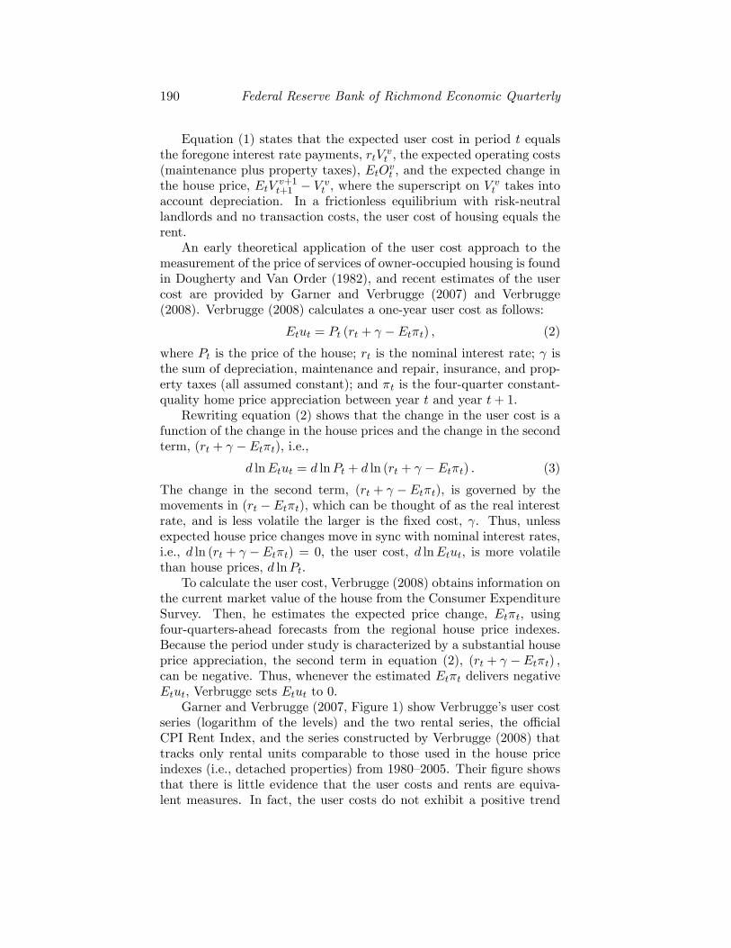
190 Federal Reserve Bank of Richmond Economic Quarterly
Equation (1) states that the expected user cost in period t equalsthe foregone interest rate payments, rtV vt , the expected operating costs(maintenance plus property taxes), EtOvt , and the expected change inthe house price, EtV v+1t+1 � V vt , where the superscript on V
vt takes into
account depreciation. In a frictionless equilibrium with risk-neutrallandlords and no transaction costs, the user cost of housing equals therent.
An early theoretical application of the user cost approach to themeasurement of the price of services of owner-occupied housing is foundin Dougherty and Van Order (1982), and recent estimates of the usercost are provided by Garner and Verbrugge (2007) and Verbrugge(2008). Verbrugge (2008) calculates a one-year user cost as follows:
Etut = Pt (rt + � Et�t) ; (2)
where Pt is the price of the house; rt is the nominal interest rate; isthe sum of depreciation, maintenance and repair, insurance, and prop-erty taxes (all assumed constant); and �t is the four-quarter constant-quality home price appreciation between year t and year t+ 1.
Rewriting equation (2) shows that the change in the user cost is afunction of the change in the house prices and the change in the secondterm, (rt + � Et�t), i.e.,
d lnEtut = d lnPt + d ln (rt + � Et�t) : (3)
The change in the second term, (rt + � Et�t), is governed by themovements in (rt � Et�t), which can be thought of as the real interestrate, and is less volatile the larger is the �xed cost, . Thus, unlessexpected house price changes move in sync with nominal interest rates,i.e., d ln (rt + � Et�t) = 0, the user cost, d lnEtut, is more volatilethan house prices, d lnPt.
To calculate the user cost, Verbrugge (2008) obtains information onthe current market value of the house from the Consumer ExpenditureSurvey. Then, he estimates the expected price change, Et�t, usingfour-quarters-ahead forecasts from the regional house price indexes.Because the period under study is characterized by a substantial houseprice appreciation, the second term in equation (2), (rt + � Et�t) ;can be negative. Thus, whenever the estimated Et�t delivers negativeEtut, Verbrugge sets Etut to 0.
Garner and Verbrugge (2007, Figure 1) show Verbrugge�s user costseries (logarithm of the levels) and the two rental series, the o¢ cialCPI Rent Index, and the series constructed by Verbrugge (2008) thattracks only rental units comparable to those used in the house priceindexes (i.e., detached properties) from 1980�2005. Their �gure showsthat there is little evidence that the user costs and rents are equiva-lent measures. In fact, the user costs do not exhibit a positive trend
M. Kudlyak: Housing Services Price In ation 191
observed in rents. After 1997, the rent series are higher than the usercost series; this suggests that owning is cheaper than renting and canexplain the increase in the homeownership rates during that period.However, it also suggests the presence of non-exploited arbitrage orlarge transaction costs of converting owner units into rentals.
The fact that house prices were rising steadily over the period up to2005 while the user cost shows no such trend suggests that the move-ments in the user cost were dominated by the movements in the secondterm in equation (2). As Garner and Verbrugge (2007) note, expectedhouse price appreciation is responsible for user cost not tracking therise in house prices. Importantly, Verbrugge (2008) notes that if insteadof the forecast house price changes, dEt�t, the expected CPI in�ationis used, then the user cost measure is much closer to the rent indexmeasure. Poole, Ptacek, and Verbrugge (2005) revisit the user cost ap-proach to examine whether the user cost can re�ect the rapidly risinghouse prices in 2005. They conclude that the user cost approach wouldnot mirror the increase in house prices.
The literature lists the following factors that can explain possi-ble divergence of the user costs and rents: (i) rent stickiness duringthe tenant�s tenure with the landlord, even beyond one-year rent con-tracts; (ii) the thinnest of the rental market for luxury homes; and (iii)the di¤erential tax treatments. For example, Diaz and Luengo-Prado(2008) show that a rental equivalence approach, as compared to a usercost approach, overestimates the cost of shelter services provided byowner-occupied housing because owner-occupied housing services arenot taxed and mortgage interest payments are deductible.
The Bureau of Economic Analysis and the BLS attempted to de-velop the user cost approach in the 1980s. However, these attemptswere abandoned because the researchers concluded that it was impos-sible to estimate the user cost without directly or indirectly using therent information (Gillingham [1980]; see a discussion in Diewert andNakamura [2009]). Summarizing, despite the fact that the user costapproach is (arguably) conceptually more attractive for the measure-ment of the price of the �ow of services provided by an asset, theapproach has proved hard to implement in practice.
One way to modify the expression for the user cost is to recognizethat the owners usually have a mortgage on the house and distinguishbetween the return on equity and the mortgage interest rate in equation(1). Early implementations of the mortgage payments in the price ofthe housing services provided by owner-occupied housing are studiedby Kearl (1979) and Gillingham (1980).
Diewert and Nakamura (2009) incorporate debt into an alternativeapproach that explicitly takes into account the �nancing of the house
192 Federal Reserve Bank of Richmond Economic Quarterly
purchase, which they refer to as the opportunity cost approach. Theyseek to compare the implications for homeowner wealth of selling theproperty at the beginning of a period with an alternative of planning tokeep the house for m more years and then either renting or occupyingfor the coming year. The opportunity cost is de�ned as the greater ofthe rental opportunity cost (which is an implicit rent) and the ��nan-cial opportunity cost.�Thus, there is never an issue of running into anegative �nancial opportunity cost.
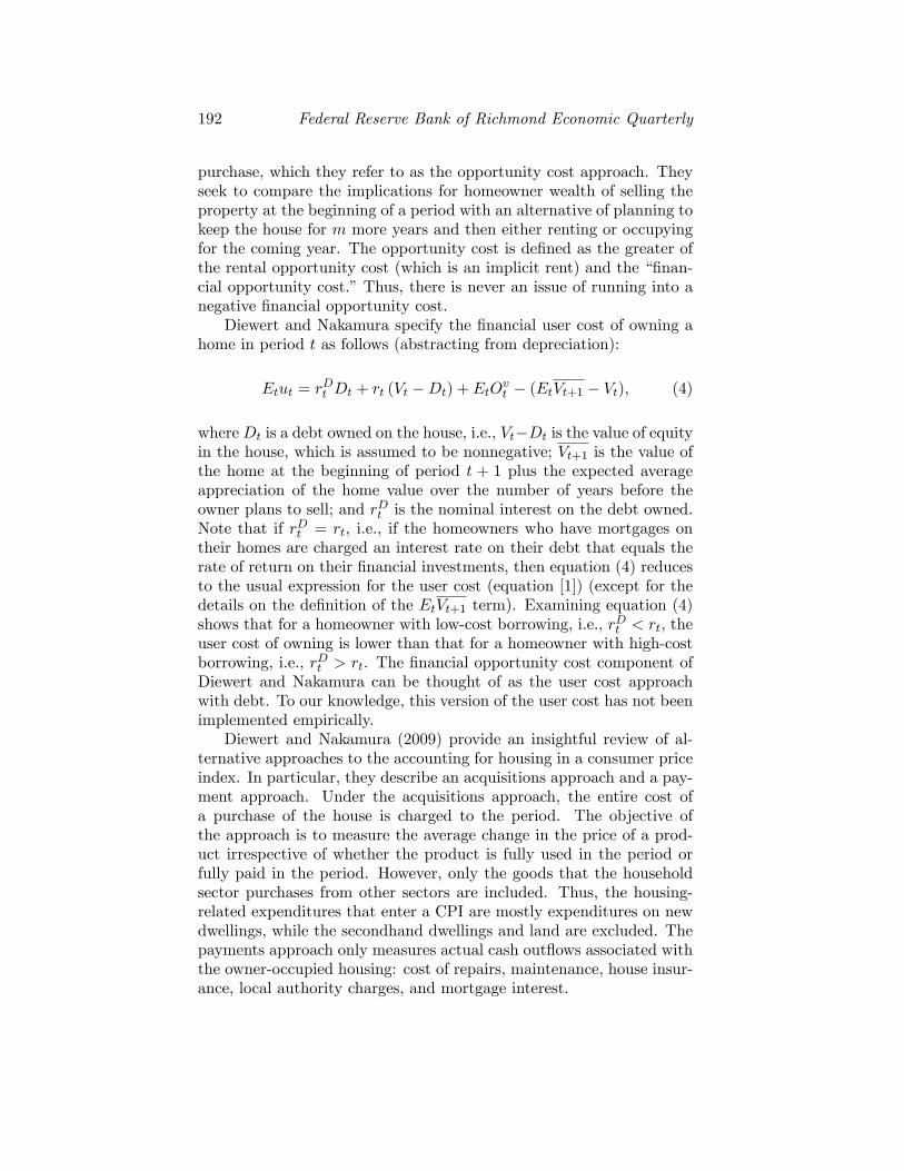
Diewert and Nakamura specify the �nancial user cost of owning ahome in period t as follows (abstracting from depreciation):
whereDt is a debt owned on the house, i.e., Vt�Dt is the value of equityin the house, which is assumed to be nonnegative; Vt+1 is the value ofthe home at the beginning of period t + 1 plus the expected averageappreciation of the home value over the number of years before theowner plans to sell; and rDt is the nominal interest on the debt owned.Note that if rDt = rt, i.e., if the homeowners who have mortgages ontheir homes are charged an interest rate on their debt that equals therate of return on their �nancial investments, then equation (4) reducesto the usual expression for the user cost (equation [1]) (except for thedetails on the de�nition of the EtVt+1 term). Examining equation (4)shows that for a homeowner with low-cost borrowing, i.e., rDt < rt, theuser cost of owning is lower than that for a homeowner with high-costborrowing, i.e., rDt > rt. The �nancial opportunity cost component ofDiewert and Nakamura can be thought of as the user cost approachwith debt. To our knowledge, this version of the user cost has not beenimplemented empirically.
Diewert and Nakamura (2009) provide an insightful review of al-ternative approaches to the accounting for housing in a consumer priceindex. In particular, they describe an acquisitions approach and a pay-ment approach. Under the acquisitions approach, the entire cost ofa purchase of the house is charged to the period. The objective ofthe approach is to measure the average change in the price of a prod-uct irrespective of whether the product is fully used in the period orfully paid in the period. However, only the goods that the householdsector purchases from other sectors are included. Thus, the housing-related expenditures that enter a CPI are mostly expenditures on newdwellings, while the secondhand dwellings and land are excluded. Thepayments approach only measures actual cash out�ows associated withthe owner-occupied housing: cost of repairs, maintenance, house insur-ance, local authority charges, and mortgage interest.
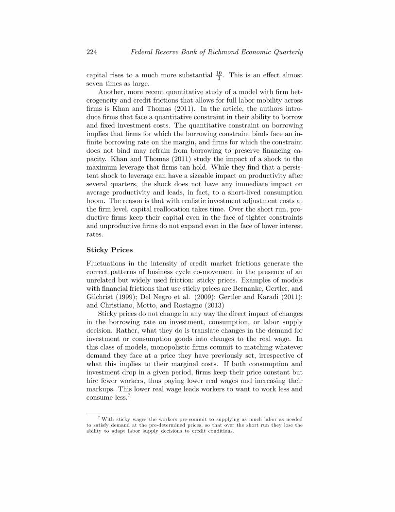
Expenditure Category and Items Expenditure Share,March 2012
Food and Beverages 15.11Housing 40.59Shelter 31.26Rent of Primary Residence 6.49Lodging Away from Home 0.81Owners�Equivalent Rent of Residences 23.66Owners�Equivalent Rent of Primary Residence 22.29
Tenants� and Household Insurance 0.34Fuels and Utilities 5.26Household Energy 4.10Water and Sewer and Trash Collection Services 1.16
Household Furnishings and Operations 4.07Apparel 3.61Transportation 17.58Medical Care 7.05Recreation 6.01Education and Communication 6.71Other Goods and Services 3.34
Notes: Category �Other Goods and Services� includes tobacco, smoking products,and personal care.
Source: BLS
2. HOUSING SERVICES PRICE INFLATION
CPI Measures of Housing Services PriceIn ation and CPI In ation
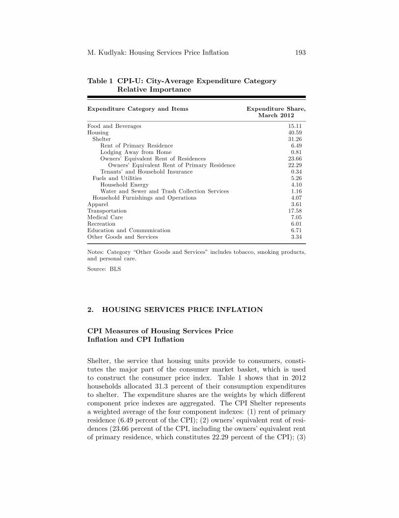
Shelter, the service that housing units provide to consumers, consti-tutes the major part of the consumer market basket, which is usedto construct the consumer price index. Table 1 shows that in 2012households allocated 31.3 percent of their consumption expendituresto shelter. The expenditure shares are the weights by which di¤erentcomponent price indexes are aggregated. The CPI Shelter representsa weighted average of the four component indexes: (1) rent of primaryresidence (6.49 percent of the CPI); (2) owners�equivalent rent of resi-dences (23.66 percent of the CPI, including the owners�equivalent rentof primary residence, which constitutes 22.29 percent of the CPI); (3)
194 Federal Reserve Bank of Richmond Economic Quarterly
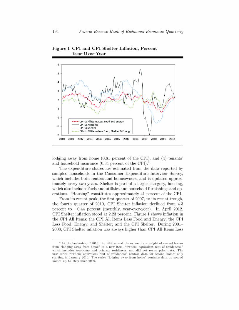
Figure 1 CPI and CPI Shelter In ation, PercentYear-Over-Year
lodging away from home (0.81 percent of the CPI); and (4) tenants�and household insurance (0.34 percent of the CPI).4
The expenditure shares are estimated from the data reported bysampled households in the Consumer Expenditure Interview Survey,which includes both renters and homeowners, and is updated approx-imately every two years. Shelter is part of a larger category, housing,which also includes fuels and utilities and household furnishings and op-erations. �Housing�constitutes approximately 41 percent of the CPI.
From its recent peak, the �rst quarter of 2007, to its recent trough,the fourth quarter of 2010, CPI Shelter in�ation declined from 4.3percent to �0.44 percent (monthly, year-over-year). In April 2012,CPI Shelter in�ation stood at 2.23 percent. Figure 1 shows in�ation inthe CPI All Items; the CPI All Items Less Food and Energy; the CPILess Food, Energy, and Shelter; and the CPI Shelter. During 2001�2008, CPI Shelter in�ation was always higher than CPI All Items Less
4 At the beginning of 2010, the BLS moved the expenditure weight of second homesfrom �lodging away from home� to a new item, �owners� equivalent rent of residences,�which includes secondary and primary residences, and did not revise prior data. Thenew series �owners� equivalent rent of residences� contain data for second homes onlystarting in January 2010. The series �lodging away from home� contains data on secondhomes up to December 2009.
M. Kudlyak: Housing Services Price In ation 195
Figure 2 Contribution of CPI Shelter In ation to Core CPIIn ation, Year-Over-Year
Source: Author�s calculations using BLS data.
Food and Energy In�ation (hereafter, core CPI in�ation). However,from the fourth quarter of 2008 up until the �rst quarter of 2012, thesituation is reversed: Core CPI in�ation exceeds CPI Shelter in�ation.
Figure 2 shows the contribution of CPI Shelter in�ation to core CPIin�ation calculated as a product of the CPI Shelter weight in the coreCPI and its year-over-year in�ation rate. The �gure shows that CPIShelter in�ation contributed 1.38 percent out of 2.63 percent of coreCPI in�ation in the �rst quarter of 2007. The contribution proceededto decline until it became negative in 2010. The contribution of CPIShelter to core CPI in�ation has been steadily increasing since then.
Table 2 shows the change in consumer price index in�ation by majorexpenditure category during the Great Recession, from December 2007to June 2009, and its aftermath, from June 2009 to April 2012.
196Federal
Reserve
Bank
ofRichm
ondEconom
icQuarterly
Table 2 Change of In ation During the Great Recession andits Aftermath, by Major Expenditure Category,Percent
Expenditure Category and Items December 2007� June 2009�June 2009 April 2012
CPI-U: All Items 1.56 6.73CPI-U: All Items Less Shelter 1.22 8.65CPI-U: All Items Less Food, Shelter, and Energy 3.23 5.60Food and Beverages 5.27 7.04Housing 2.10 2.58Shelter 2.25 2.78Rent of Primary Residence 4.38 3.82Lodging Away from Home �8.28 7.83Owners�Equivalent Rent of Residences 2.99 2.68Owners�Equivalent Rent of Primary Residence 2.99 2.68
Fuels and Utilities 1.00 6.07Household Energy �0.74 3.53Water and Sewer and Trash Collection Services 9.18 16.13
Household Furnishings and Operations 2.26 �2.59Apparel 0.76 4.49Transportation �6.52 20.70Medical Care 4.53 9.46Recreation 2.29 �0.07Education and Communication 4.97 4.73Other Goods and Services 9.73 5.22
Notes: Author�s calculations using BLS data.
M. Kudlyak: Housing Services Price In ation 197
Figure 3 CPI Rent In ation, CPI OER In ation, and HousePrice In ation, Year-Over-Year
CPI Measures of Housing Services PriceIn ation and House Prices
As can be seen from Table 1, the main components of the CPI Shel-ter are the CPI Rent of Primary Residence (CPI Rent) and the CPIOwners� Equivalent Rent of Primary Residence (CPI OER). Figure3 shows CPI Rent in�ation and CPI OER in�ation along with in�a-tion in house prices as measured by the Core Logic house price indexand the Federal Housing Finance Agency Purchase Only Index (seeFigure 4).
Figure 3 shows that house price in�ation �uctuates signi�cantlymore than CPI Rent or CPI OER in�ation. It is especially evidentduring 2004�2010. The �gure also shows that house price in�ationand in�ation in the CPI measures of housing often do not move in thesame direction. Between 2002 and 2004, house price in�ation was risingwhile in�ation in the CPI housing indexes was falling. During 2005�2009, when house price in�ation rapidly fell from 15�20 percent in 2005to �15 to �20 percent in 2009, CPI housing in�ation was �uctuatingaround 4 percent and started decreasing only after 2008.
The periods when the CPI measure of in�ation diverges particularlyfar from house price in�ation often reignite a debate about whetherthe CPI Rent and CPI OER adequately re�ect the cost of shelter. Asemphasized in Section 1, it is important to recognize that the cost of
198 Federal Reserve Bank of Richmond Economic Quarterly
Figure 4 CPI Rent, CPI OER, and the Rent and HousePrice Indexes
Notes: Q1:2004 = 100.
Source: Author�s calculations using BLS data.
housing services should not necessarily move with house prices. TheCPI program�s indexes of housing in�ation measure in�ation in theprices of housing services rather than in�ation in house prices. Giventhe method that the BLS currently uses to measure the cost of thehousings services of owner-occupied units, house prices are re�ected inthe CPI index to the extent that they are re�ected in the current rent inthe ongoing rent contracts (via the supply and demand of rental unitsand the substitution between renting and owning). Alternatively, theuser cost approach to measuring the cost of owner-occupied housingshows more directly that the cost of shelter depends both on currenthouse prices and on their expected change.
3. RECENT DEVELOPMENTS IN THE RENTALHOUSING MARKET
As described above, the current accounting for price of housing servicesin the CPI almost entirely relies on the data on rental prices from rentalunits. In addition, the monthly price changes used for calculation of thein�ation in the price of housing services is the monthly average of theprice change over the last half year. Thus, a direct examination of the
M. Kudlyak: Housing Services Price In ation 199
recent developments in the rental market can be useful in gauging thedirection of changes of housing services price in�ation. Recently, newdata series that describe the aggregate rental market became available.In contrast to the CPI housing services price indexes, these series re�ectmonth-to-month changes and, thus, can serve as leading indicators ofthe changes in rental prices. In this section, we describe the behavior ofdi¤erent indicators of the rental market and the behavior of alternativemeasures of rent price in�ation.
Additional Indicators of the Rental Market
Rent Concessions
One way to gauge the pressure on rent prices is to examine the seriesof discounts that landlords are willing to extend to renters. Figure 5shows the di¤erence between the asking rent and the e¤ective rent as ashare of asking rent obtained from Reis Inc. The larger the di¤erence,the more concessions a landlord is willing to provide to a renter. The�gure shows that the discount is at its lowest level of the last 10 years.It has declined from its peak of 6.3 percent in the second quarter of2009 to 4.8 percent in the �rst quarter of 2012. Reis Inc. forecasts afurther decline in concessions to 3.23 percent by 2016.
Figure 5 also shows the share of properties o¤ering a discount andthe average discount in the annual rent, the series obtained from CBRichard Ellis (hereafter, CBRE). The share of properties o¤ering adiscount has declined from approximately 47 percent in the �rst quarterof 2010 to 19 percent in the �rst quarter of 2012. The average annualdiscount has also been declining during this period.
Rental Vacancy Rates and Net Absorption
An alternative way to examine the direction of the pressure on the rentprices is to examine the supply of the properties available for rent. Thevacancy rate for renter-occupied housing is de�ned as the number ofvacant units for rent over the stock of vacant and occupied units forrent. Figure 6 shows the vacancy rate series from the Census, CBRE,and Reis Inc. The three series show a decline in the vacancy ratessince mid-2009. In particular, Reis data show that the vacancy ratehas declined from 8 percent in mid-2009 to 4.9 percent in the �rstquarter of 2012.
The net absorption, NAt, as measured by Reis Inc., is the di¤erencebetween the occupied stock of rental units in the current period, Ot,and in the last period, Ot�1; which is the di¤erence between the numberof newly signed leases and the number of leases that were terminated
200 Federal Reserve Bank of Richmond Economic Quarterly
Figure 5 Measures of Rent Discounts
Notes: Concessions are the ratio of the di¤erence between asking rent and e¤ectiverent to the asking rent. Markers indicate annual observations.
Source: CBRE and Reis Inc.
and not renewed, NAt � Ot � Ot�1 = NRt � TRt. Figure 7 showsthe net absorption as a share of the previous period stock of occupiedrental vacancies. As can be seen from the �gure, after mid-2008 thenet absorption has been positive and increasing since 2011.
The increase in the net absorptions has been feeding into the recentrapid decline in vacancy rates. To see this, note that the evolution ofthe number of vacancies, vt, can be described by the following equation
vt = vt�1 + (NComplt +NConvt)�NRt + TRt; (5)
where NComplt is the number of new completions and NConvt is thenumber of net conversions into the rental units.
Assuming that the change in the stock of rental properties fromt � 1 to t is negligible as compared to the change in the number ofvacancies, equation (5) shows that the decrease in the vacancy ratefrom t � 1 to t can be brought by a decrease in net completions, adecrease in net conversions, or by an increase in the net number ofnewly signed rental contracts, (NRt � TRt). Reis Inc. predicts anincrease in net completions from 39,400 properties in 2011 to 66,500
M. Kudlyak: Housing Services Price In ation 201
Figure 6 Rental Vacancy Rates
Source: Census Bureau, CBRE, and Reis Inc.
properties in 2012. Given the negligible role of net conversions, thedecrease in the vacancy rent is mostly because of an increased demandfor rental units.
The series of the rental vacancy rates and the rent concessions sug-gest that there is an upward pressure on the rent prices.
Alternative Indicators of Rent Price In ation
There are two alternative rent indexes that measure aggregate rentin�ation. The �rst index is the REIS Rent Index, which is providedby Reis Inc. The second index is the CBRE Rent Index, provided byCBRE. Reis Inc. collects data on the asking rent, Reis Asking rent,and on the e¤ective rent in newly signed leases, Reis E¤ective rent.The rent data do not include information from the renewed leases andReis Inc. does not collect information on the rents in ongoing leasecontracts. The rent information for the CBRE Rent Index is obtainedby asking the managers of the properties about what the rent wouldbe if they were to rent a unit in the current market, regardless ofwhether the unit is currently occupied or vacant. Thus, the recodedinformation might be on the rents in ongoing contracts as well as on the
202 Federal Reserve Bank of Richmond Economic Quarterly
Figure 7 Net Absorptions of Rental Properties
Notes: The �gure shows net absorptions as the share of the previous period stockof occupied rental units. Net absorption is the di¤erence between the occupiedstock of rental units in the current period and the occupied stock in the previousperiod. The �gure shows annual observations prior to 2007 and quarterly obser-vations thereafter. The dotted line indicates forecast.
Source: Reis Inc.
perceived e¤ective new rents. Thus, both indexes contain informationabout month-to-month changes in rental prices.
The Reis Asking rent and the CBRE Rent Index both provide infor-mation on the apartment rents in the multi-housing market, with somedi¤erences in the coverage. Data from Reis Inc. cover rental complexesconsisting of 40 or more units (except for California metropolitan ar-eas, where complexes of 15 or more units are included). Data for theCBRE Rent Index cover multi-housing properties with �ve or moreunits.5 Housing data from the U.S. Census Bureau has a much widerscope. The Census uses residential properties regardless of rent restric-tions and does not have a restriction on the number of rental units.The CPI Rent also includes data on rent-controlled properties.
Figure 8 shows quarterly year-over-year in�ation in the CPI Rent,the CPI OER, the Reis E¤ective rent, and the CBRE Rent. All fourin�ation series show a decline during the 2001 and 2007�2009 recessions.The �gure suggests that Reis Rent Index in�ation and CBRE Rentin�ation appear to lead the CPI Rent and CPI OER in�ation measures.
5 This information was obtained from CBRE and Reis Inc. representatives inJune 2011.
M. Kudlyak: Housing Services Price In ation 203
Figure 8 Rent In ation
Source: BLS, CBRE, and Reis Inc.
A particularly striking feature of Figure 8 is that Reis Rent Indexin�ation and CBRE Rent in�ation experienced a signi�cantly largerdrop during 2007�2009 as compared to the CPI in�ation measures.Such a discrepancy between Reis Rent Index in�ation or CBRE Rentin�ation and the CPI housing services in�ation can, at least partially,be attributed to the di¤erent time reference period of these measures.Recall from Section 1 that the CPI month-to-month housing servicesprice in�ation measure essentially represents a monthly average overthe past six-month change, while Reis Rent Index in�ation and CBRERent in�ation represent month-to-month changes.
In�ation as measured by the CBRE Rent Index has been increasingfrom its recent trough of �4.95 percent in the fourth quarter of 2009to 4.67 percent in the �rst quarter of 2012. During the same period,in�ation as measured by the Reis Rent Index has increased from itstrough of �2.92 percent to 2.83 percent in the �rst quarter of 2012. CPIRent in�ation and CPI OER in�ation lagged the other two in�ationmeasures and reached their troughs, at 0 percent and �0.2 percent,respectively, in the second quarter of 2010. CPI Rent in�ation standsat 2.5 percent and CPI OER in�ation stands at 1.9 percent in the �rstquarter of 2012.
204 Federal Reserve Bank of Richmond Economic Quarterly
4. CONCLUSIONS
The CPI is a cost of living index that measures the price of a constant�ow of consumption during a period. One of the challenges of account-ing for the price of consumption is accounting for the price of housingservices. The issue is that a large fraction of the U.S. population ownstheir housing. The price of housing services for owner-occupied hous-ing is not observed directly and, thus, the price for the hypotheticalmarket transaction involving the housing services of owner-occupiedhousing must be imputed.
The Bureau of Labor Statistics employs a particular imputationmechanism, the rental equivalence approach, which implies a close sub-stitutability between rental and owner-occupied housing. An alterna-tive, conceptually more attractive approach to accounting for the priceof the �ow of services provided by an asset (i.e., by a house) is the usercost approach. Despite its conceptual attractiveness, the approach hasproven hard to implement in practice.
Currently, the monthly CPI measures of housing services price in-�ation represent a repeat-rent index, which is calculated as the monthlyaverage of the past six-month change of the rental price of rental units.The newly available data from the rental housing market, which usuallyre�ects month-to-month changes, can be informative about the direc-tion of changes in the CPI measure of housing services in�ation. Thedata on residential rents, rental vacancies, and rent concessions suggestthat since 2010 there has been an increasing upward pressure on rentprice in�ation.
APPENDIX
Below, we describe (1) how the data on rental prices are collected, and(2) how the data are used to construct the CPI Rent and the CPI OER.
The collection of rent information for construction of the CPI Rentand CPI OER is conducted as follows. The CPI program collects priceinformation from 87 urban areas (i.e., index areas). Each of the indexareas is divided into six strata, each representative of the area. Withineach stratum, the program de�nes small segments. For each segment,the CPI program collects information on the number of renter- andowner-occupied units, and the average rent of renter units. Based onthis information, the program calculates the total spending on shel-ter for each segment. The total spending on shelter is the sum of (1)
M. Kudlyak: Housing Services Price In ation 205
the product of the number of rental units and the average rent in thesegment, and (2) the product of the number of owned units and theaverage owner�s equivalent of rent in the segment. The segments in thestratum are selected with the probability proportional to the segment�ssize, where the size of the segment corresponds to the segment�s esti-mated total spending on shelter. Finally, the CPI program selects arepresentative sample of renters in each segment.
The rental units in each of the six strata are interviewed every sixmonths on a panel basis. One of the six panels is priced each monthand each panel is priced twice per year. Thus, the month-to-monthprice changes in housing services are calculated using the six-monthchanges in rents.
From each rental unit in the sample, information on the economicrent and on the pure rent is collected. The economic rent is the contractrent (including the value of certain rent reductions) adjusted by thevalue of any changes in the services the landlord provides. A change inwhat renters obtain for their rents is considered to be a quality change,and the value of any quality change is applied to the current economicrent to make it consistent with the previous data. The pure rent is usedin calculations of the owners�equivalent of rent. It is the economic rentminus any utilities included in the contract rent. The utilities paid byhomeowners are counted outside the CPI Shelter.
To construct the CPI Rent and CPI OER, the CPI program usesthe so-called price relatives. The price relative is the ratio of (weighted)prices from the current month to the (weighted) prices in the previousmonth. Since each housing unit is interviewed every six months, themonthly price relative is the sixth root of the six-month price change.For example, the six-month change in rent for all renter-occupied unitsin a segment is the ratio of (1) the sum of the current economic rentsfor each sampled unit within the segment, weighted by the total renterweight for that segment, and (2) the sum of the economic rents chargedsix months ago for each sampled unit within the segment, weighted bythe total renter weight for that segment. The total renter weight in asegment is the product of the segment�s weight, the renters�share in thetotal renter- and owner-occupied spending on shelter in the segment,and the inverse of the probability of a housing unit in the segment to beselected to the sample. The latter corrects for the sampling design. Thesegment�s weight is the inverse of the probability of its being included inthe stratum, where the probability is the ratio of the total spending onshelter in the segment to the total spending on shelter in the stratum.
Consider rental unit i in segment s, which is located in pricing areaa. Let Ws denote the segment�s s weight. Let Ss denote the renters�share in the total renter- and owner-occupied spending on shelter in
206 Federal Reserve Bank of Richmond Economic Quarterly
segment s. Let ps denote the probability of a unit in segment s to beselected to the sample. Then, the monthly relative price change for theCPI Rent for area a, �t�1;ta;rent, is
�t�1;ta;rent =6
vuuut Pi2a
h�Ws
Ssps
�econ renti;t
iPi2a
h�Ws
Ssps
�econ renti;t�6
i :The monthly relative price change for the OER index for area a,�t�1;ta;OER,is
�t�1;ta;OER =6
vuuut Pi2a
h�Ws
1�Ssps
�pure renti;t
iPi2a
h�Ws
1�Ssps
�pure renti;t�6
i :Then, the CPI Rent and the CPI OER for area a are calculated as
follows:
Ita;rent = It�1a;rent�t�1;ta;rent
Ita;OER = It�1a;OER�t�1;ta;OER:
These measures are then used to aggregate the indexes across all CPIindex areas.
REFERENCES
Bureau of Labor Statistics. 2007. �The Consumer Price Index.�Available at www.bls.gov/opub/hom/pdf/homch17.pdf.
Bureau of Labor Statistics. 2009. �How the CPI Measures PriceChanges of Owners�Equivalent Rent of Primary Residence (OER)and Rent of Primary Residence (Rent).�Available atwww.bls.gov/cpi/cpifacnewrent.pdf (April).
Crone, Theodore M., Leonard I. Nakamura, and Richard Voith. 2010.�Rents Have Been Rising, Not Falling, in the Postwar Period.�The Review of Economics and Statistics 92 (August): 628�42.
Diaz, Antonia, and Maria Jose Luengo-Prado. 2008. �On the UserCost and Homeownership.�Review of Economic Dynamics 11(July): 584�613.
Diewert, W. Ervin, and Alice O. Nakamura. 2009. �Accounting forHousing in a CPI.�The Federal Reserve Bank of PhiladelphiaWorking Paper No. 09-4 (March).
M. Kudlyak: Housing Services Price In ation 207
Diewert, W. Ervin, and Alice O. Nakamura, and Leonard I.Nakamura. 2009. �The Housing Bubble and a New Approach toAccounting for Housing in a CPI.�Journal of Housing Economics18 (September): 156�71.
Dougherty, Ann, and Robert Van Order. 1982. �In�ation, HousingCosts, and the Consumer Price Index.�American EconomicReview 72 (March): 154�64.
Garner, Thesia I., and Randal Verbrugge. 2007. �The PuzzlingDivergence of U.S. Rents and User Costs, 1980�2004: Summaryand Extensions.�Bureau of Labor Statistics Working Paper No.409 (October).
Genesove, David. 2003. �The Nominal Rigidity of Apartment Rents.�Review of Economics and Statistics 85 (November): 844�53.
Gillingham, Robert. 1980. �Estimating the User Cost ofOwner-Occupied Housing.�Monthly Labor Review 103 (2): 31�5.
Kearl, J. R. 1979. �In�ation, Mortgage, and Housing.�Journal ofPolitical Economy 87 (October): 1,115�38.
Kudlyak, Marianna. 2009. �The Cyclicality of the User Cost of Laborwith Search and Matching.�Federal Reserve Bank of RichmondWorking Paper No. 09-12.
Poole, Robert, Frank Ptacek, and Randal Verbrugge. 2005.�Treatment of Owner-Occupied Housing in the CPI.�Bureau ofLabor Statistics Working Paper, presented to the FederalEconomic Statistics Advisory Committee (December).
Prescott, Edward C. 1997. �On De�ning Real Consumption.�TheFederal Reserve Bank of St. Louis Review May: 47�53.
Verbrugge, Randall. 2008. �The Puzzling Divergence of Rents andUser Costs, 1980�2004.�Review of Income and Wealth 54(December): 671�99.
Wolman, Alexander L. 2011. �K-Core In�ation.�Federal ReserveBank of Richmond Economic Quarterly 97 (4): 415�30.
Economic Quarterly� Volume 98, Number 3� Third Quarter 2012� Pages 209�230
When Do Credit FrictionsMatter for Business Cycles?
Felipe Schwartzman
The Great Recession took a turn for the worse in October 2008,at the same time as the collapse of Lehman Brothers. Manyresearchers viewed this con�uence of events as evidence that
credit frictions� disfunction in credit markets that distort the cost ofintertemporal trade� were, if not the ultimate cause, at least a keymechanism that made the recession much deeper and more prolongedthan it would otherwise have been.1 As a consequence, there has beenrenewed interest in constructing macroeconomic models that are ableto capture this idea (see Kiyotaki and Gertler [2011], Quadrini [2011],and Brunnermeier, Eisenbach, and Sannikov [2012] for recent reviewsof that literature).
One di¢ culty that stems from that view is that adding credit fric-tions to an otherwise standard frictionless general equilibrium businesscycle model is not necessarily su¢ cient to generate dynamics that arequantitatively or even qualitatively compatible with actual businesscycles. The reasons behind this di¢ culty are fairly general, and stemfrom the fact that most models of credit frictions normally work bydistorting the terms of inter-temporal tradeo¤ faced by �rms or house-holds. However, as we will see, realistic business cycle dynamics requireshocks to a¤ect intra-temporal labor supply decisions.
In order for models with credit frictions to generate compellingresults, it is necessary to depart from more conventional ways of mod-elling preferences and technology, for example by adding a capacity
The views expressed here do not necessarily re�ect those of the Fed-eral Reserve Bank of Richmond or the Federal Reserve System. E-mail:[email protected].
1 See Campello, Graham, and Harvey (2010); Ivashina and Scharfstein (2010); andPuri, Rocholl, and Ste¤en (2011) for empirical articles that establish the link betweenchanges in credit conditions over that period and production decisions.
210 Federal Reserve Bank of Richmond Economic Quarterly
utilization margin, by introducing working capital requirements, or byallowing for �rm-level heterogeneity. Furthermore, credit frictions canplay a more realistic role in the presence of additional frictions, such assticky prices and incomplete contracts. This article is a guide to thesemodi�cations, explaining how they work, why they are necessary, andhow they can be motivated
The identi�cation of credit frictions with distortions to the in-tertemporal tradeo¤s faced by particular agents allows us to cover alarge part of the literature, but not all of it. The last section of thisarticle discusses a couple of recent examples in the literature wherecredit frictions act instead by a¤ecting agents� risk management op-portunities and bargaining position. This line of research is promisingexactly because it sidesteps a lot of the di¢ culties associated with aheavy reliance on intertemporal distortions.
As with any literature review, this is by necessity limited in scope.The focus is on articles that strive to make a quantitative point, ratherthan only exposing a qualitative mechanism. Furthermore, we do notdiscuss the vast literature about what exactly gives rise to these fric-tions, rather, taking as given that they might become more importantin certain instances and tracking down what this implies.
We proceed as follows: First, we motivate interpreting credit fric-tions as a tax on intertemporal trade. This is a simpli�cation that willbe useful for the rest of the text, since it will allow us to focus sharplyon the impact of credit frictions on the decisions of households and ofnon-�nancial �rms while abstracting from the precise mechanism thatgives rise to those frictions. We then review two ways in which gen-eral equilibrium considerations can limit the impact of credit frictions.The �rst is that changes in the demand for physical capital inducedby changes in the intensity of credit frictions only translates into asigni�cantly lower capital stock over a long period of time. Second,changes in intertemporal tradeo¤s faced by households often lead themto increase consumption as they reduce labor supply and vice versa.We then discuss extensions and modi�cations to the baseline modelthat help mitigate or reverse some of these e¤ects. The last sectionconcludes.
1. CREDIT FRICTIONS AS A TAX ONINTERTEMPORAL TRADE
Credit frictions appear in many forms. They can originate from asym-metric information (as in Bernanke and Gertler [1989]) or from lim-ited commitment problems (as in Kiyotaki and Moore [1997]), andmay show up in the data as quantitative limits on borrowing, down
F. Schwartzman: When Do Credit Frictions Matter? 211
payment or margin requirements, non-linear pricing for debt, and out-right exclusion of particular agents from credit markets. All of theseforms have one feature in common: The agents directly a¤ected behaveas if they were subject to a tax on borrowing, e¤ectively applying totheir decisions interest rates that are higher than if they were not sub-ject to the friction. Furthermore, in the same way as a tax on credit,credit frictions impact equilibrium interest rates, which also impactagents who are not subject to the underlying commitment or informa-tional problems.
In that spirit, much of this article will take a reduced form approachto credit frictions, equating variations in the intensity of the frictionwith variations in the �after tax� interest rate faced by borrowers orthe �before tax�rate faced by lenders. The reduced form approach isappropriate given that the purpose of the article is to describe modeldynamics rather than to discuss policy. It has the added advantageof putting the focus sharply on the reaction of individual agents tochanges in the credit frictions as opposed to the details about howthey are determined.
In many instances it will be useful to take a partial equilibrium ap-proach, to take other prices as given when discussing the impact of thechange in the after tax interest rate on an agent�s decision. This shouldcapture the primary impact of credit frictions in most of the modelsunder review. In some important instances a full comprehension of themechanism will also require referring to general equilibrium e¤ects. Wewill address these as needed.
The interpretation of credit frictions as a tax on borrowing is in linewith the interpretation given by Chari, Kehoe, and McGrattan (2005)and, in policy circles, is used by the Estimated, Dynamic, Optimization-based Model of the U.S. Economy used by the Federal Reserve Board(see Chung, Kiley, and Laforte [2010]). Chari, Kehoe, andMcGrattan (2005) discuss how the canonical models with credit fric-tions by Bernanke and Gertler (1989), Carlstrom and Fuerst (1997),and Kiyotaki and Moore (1997) can be reinterpreted as models of thedetermination of a tax on borrowing. In these models, the tax wedgeappears as one operating between households, who save, and �rms, whoborrow. In richer environments with �rm or household heterogeneity,the tax wedge can also appear as di¤erences in the interest rate facedby di¤erent �rms or di¤erent households (see Buera and Moll [2012]for a discussion).
When bringing the models to the data, it is important to rememberthat from the perspective of individual agents, changes in this tax wedgecan appear either as a change in the risk premium paid by an agenton her loans, or, given a quantitative limit on debt, as an increase in
212 Federal Reserve Bank of Richmond Economic Quarterly
the shadow cost of funds. Therefore, the intensity of credit frictionsare not well-measured by the riskless interest rate paid by the U.S.Treasury or the overnight interest rate paid in interbank markets, bothof which often drop in recessions. Rather, they are best measured by awide spectrum of credit indicators that are strongly pro-cyclical such ascredit �ows, the fraction of senior bank managers who report tighteningof credit standards, and spreads between bonds with di¤erent ratings(see Quadrini [2011] for a discussion of these indicators).
Not all the e¤ects of credit frictions can be easily summarized witha tax on credit relationships. In the last section we examine two cases ofrecent articles where the most interesting e¤ects of the credit frictionsare unrelated to that particular aspect.
2. PROBLEMS FOR MODELS WITHCREDIT FRICTIONS
Take a basic real business cycle model such as King, Plosser, andRebelo (1988) and add credit frictions to it. Most likely, these fric-tions are going to either imply counterfactual dynamics or will mattervery little for aggregate �uctuations. There are two main problems:The �rst is that while investment might react strongly to increases incredit frictions, the capital stock is a slow-moving variable. Thus, forcredit frictions to matter, they need to have an impact on employment.The second problem is that the typical impact of credit frictions on em-ployment is such that employment and consumption have the wrongco-movement, with consumption booming when employment drops andvice versa. We discuss each of these problems in turn.
Problem 1: Capital Stock is Inelastic in theShort Run
Firms that face higher borrowing costs are likely to reduce their in-vestment. If nothing else, this should be one channel through whichtighter credit would lead to lower output. However, given conventionalcalibration of technology and preferences, tightening credit will onlyhave a modest impact on output through this channel.2
Over the short run, the capital stock is inelastic because buildingsand equipment in place do not become unproductive overnight for lackof replacement or maintenance. For example, suppose yearly deprecia-tion is 10 percent of capital and steady-state investment is 12 percent of
2 This is a problem originally pointed out by Kocherlakota (2000).
F. Schwartzman: When Do Credit Frictions Matter? 213
capital stock (so that capital grows by 2 percent a year). Furthermore,suppose that over the course of a year, investment drops by 18 percent,which is approximately the drop in �xed capital formation over thefour quarters starting in Q4:2008 when compared to the previous fourquarters. Then, the capital stock drops by about 0.16 percent. Witha capital elasticity of output of about 13 , this would account for a dropin output of 0.05 percent. While this is a signi�cant deviation for aneconomy that grows at 2 percent in a normal year, it cannot accountfor the almost 4 percent drop in gross domestic product that took placein the year after the collapse of Lehman Brothers.
One may wonder whether the almost 20 percent drop in investmentis an understatement, given imperfect measurement of intangible capi-tal and the violence of the crisis. As it turns out, this drop in investmentis in line with recent quantitative work by Khan and Thomas (2011),who model the impact of a credit shock on investment decisions madeby �rms. Their model includes two mechanisms that keep investmentfrom falling more substantially. First, there are adjustment costs tocapital at the �rm level. Second, consistent with empirical work thathas found little e¤ect of interest rates on household savings decisions(see Deaton [1992] for a review of that work), in equilibrium, interestrates have to drop substantially to convince households to reduce theirsavings. The drop in the interest rate, in turn, relaxes the constraintsfaced by �rms, undoing much of their e¤ect on investment. (This e¤ectis emphasized and discussed in detail by Coen-Pirani [2005].)
Problem 2: Co-Movement between LaborSupply and Consumption
Business cycle models with credit frictions will usually change thehouseholds�incentives to save. This may occur directly if householdsare subject to time varying credit frictions, as in Cúrdia and Woodford(2009), Mendoza (2010), and Guerrieri and Lorenzoni (2011), or indi-rectly if, as in Carlstrom and Fuerst (1997), changes in the intensityof credit frictions applying to �rms a¤ect the equilibrium interest ratereceived by households who lend to these �rms. Such an equilibriumadjustment is necessary since credit frictions imply that, for a giveninterest rate received by lenders, borrowers do not borrow as much asthey would otherwise. Fluctuations in the interest rate can assure thatequilibrium is maintained.
As discussed above, the empirical evidence suggests that house-hold savings are unlikely to be very elastic to interest rates or, moregenerically, to incentives for intertemporal substitution. However, tothe extent that they are, under conventional assumptions households
214 Federal Reserve Bank of Richmond Economic Quarterly
will choose to reduce labor supply at the same time that they chooseto increase consumption and vice versa. If a household faces a higherborrowing interest rate, it will choose to reduce borrowing both byconsuming less and by working longer hours to increase income.
This point is made transparently by Barro and King (1984) in aslightly di¤erent context. They investigate the impact of intertemporalprices on household behavior. Their result relies on two assumptions:1) leisure is a normal good, its demand increasing in household wealth,and 2) utility is time separable, with consumption or leisure in a giventime period having no e¤ect on the enjoyment of consumption or leisurein subsequent periods. The �rst assumption conforms to the long-run evidence that, in spite of substantial increases in wages over time,labor supply does not exhibit a strong secular trend (King, Plosser,and Rebelo 1988). The second assumption is more controversial sincemodels with habits are very common, but should be less controversialthe longer it is under consideration.
Suppose we write the intertemporal optimization problem of a house-hold as:
maxCt;Lt
1Xt=0
�tu (Ct; 1� Lt)
s:t: :1Xt=0
1
R0;t[Ct � wtLt] � B0;
with u increasing and concave in both arguments. Ct is consumption,Lt is labor supply, 1�Lt is leisure, B0 is initial wealth, wt is the rate atwhich the household can transform labor hours into consumption goods(the wage rate), and 1
R0;tis the price of time t consumption relative to
time 0 consumption. The one-period interest rate between t and t+ 1is Rt;t+1 =
R0;t+1R0;t
.We are interested in knowing how consumption and leisure change
in response to changes in the interest rate. This can be interpretedeither as the equilibrium rate faced by households or, more generallyin the case where households are directly a¤ected by credit frictions,as the �after tax� interest rate that captures the incentive impact ofthose frictions.
We can solve the problem in two steps. First, for a given savingdecision fStg1t=0 � fwtLt � Ctg1t=0, we �nd how the household opti-mally chooses consumption and labor supply. This is the solution tothe static optimization problem:
fC (St; wt) ; L (St; wt)g = arg maxCt;Lt
u (Ct; 1� Lt)
Ct + St � wtL:
F. Schwartzman: When Do Credit Frictions Matter? 215
Given the solution to the static problem, we then choose a sequenceof fStgs to solve the dynamic problem:
maxet
X�tu (C (wt; St) ; 1� L (wt; St))
s:t: :1Xt=0
1
R0;tSt � �B0;
where the constraint states that the discounted present value of savingscannot be less than the negative initial assets of the household.
It is easy to see that consumption and leisure choices only dependon the interest rate through its e¤ect on savings, St. Thus, in order tounderstand the impact of changes in credit frictions on consumptionand labor supply, we need to understand the impact of a change inSt in the static problem. We can rewrite the budget constraint of thestatic problem as:
Ct + wt (1� Lt) � wt � St:
Given the saving decision, St, and the wage rate, wt, the staticproblem has the same form as an intermediate microeconomics text-book consumer maximization problem over two goods, Ct and 1� Lt,with relative price wt and wealth given by wt � St. Since both goodsare normal, the optimal response of the household to an increase inSt is to reduce both consumption and leisure. Thus, if a householddecides to increase saving, it will both reduce consumption and increaseemployment. Negative co-movement of consumption and employmentis of course at odds with business cycle data.
How big are wealth e¤ects on labor supply likely to be? Baselinecalibrations of preferences imply that they ought to be substantial.Over a span of several decades, hours worked have moved relativelylittle when compared to the manifold increase in wages over that sameperiod. A commonly used functional that captures this fact is3
u (C;L) =
�C1�� (1� L)�
�1��1� � :
3 More generally, King, Plosser, and Rebelo (1988) show that, in order for hoursworked to remain constant over time, even as wages increase, the period utility functionof households has to be:
u (C;L) =1
1� �C1��v (1� L) or
u (C;L) = log (C) + v (1� L) :
216 Federal Reserve Bank of Richmond Economic Quarterly
The solution to the period-by-period static problem implies
�
1� �C
1� L = w;
so that L remains constant if wages and consumption grow at the samerate. A typical calibration chooses � so that L = 1
3 since this impliesthat people work approximately one-third of their available time (eighthours in a day). Applying the implicit function theorem,
dC
C= � L
1� LdL
L
= �12
dL
L:
Thus, a change in the interest rate that leads to a 1 percent dropin consumption will also generate a 2 percent rise in employment.
An instructive example of how this mechanism operates in an equi-librium environment is Chari, Kehoe, and McGrattan (2005). Thearticle studies the e¤ect of a �sudden stop� in foreign capital �owsto a small open economy. The shock takes the form of a temporaryquantitative limit in net imports from abroad. The economy accom-modates to the tightened limit with a reduction in consumption andinvestment, but an increase in employment. The sudden stop in foreigncapital �ows leads to an output boom.
Another example is Carlstrom and Fuerst (1997). They study thee¤ect of a shock to entrepreneurial wealth in a closed economy. Giventhe credit friction, the shock reduces the borrowing capacity of en-trepreneurs, forcing them to reduce investment. However, in generalequilibrium this can only be accomplished through an increase in house-hold consumption. The price change that supports this consumptionboom is a reduction in the interest rate faced by households. In re-sponse, households increase leisure and reduce employment. In sum,in response to an entrepreneurial wealth shock, the model generates arecession with a consumption boom.
One important lesson from Barro and King (1984) is that, giventheir assumptions, for shocks to generate realistic co-movement be-tween consumption and labor supply, they need to have an impact onthe wage rate, wt. In the rest of the article, we will review some of thestrategies that the literature has devised to have the wage rate movein response to credit frictions.
Summary
The analysis above also gives some hints as to which mechanismsare likely to generate realistic business cycle �uctuations. These are
F. Schwartzman: When Do Credit Frictions Matter? 217
typically mechanisms that 1) have an impact on employment and 2)a¤ect real wages. Wages can drop if a shock generates a reductionin labor productivity or if the shock acts as a tax on wages (a �laborwedge�). Such shocks will lead �rms to want to hire fewer workers and,in equilibrium, there will be a drop in wages that will induce householdsto reduce both their consumption and their leisure time.
Numerical studies of general equilibrium stochastic growth mod-els bear out this intuition, implying that productivity shocks and laborwedge shocks account for the bulk of business cycle �uctuations, includ-ing the Great Depression (see Chari, Kehoe, and McGrattan [2005] andthe various articles collected in Kehoe and Prescott [2002]), but an �in-terest rate wedge�(i.e., a tax on saving or investment) measured in asimilar way cannot account for much.
3. MODIFICATIONS OF THE STANDARD MODEL
We now turn to modi�cations to the baseline model that help increasethe potential impact of credit on the real economy.
Labor Supply
The literature on credit frictions has adopted particular functionalforms for the utility function that eliminate or greatly mitigate thewealth e¤ect on labor supply. One popular solution is to postulate autility function as in Greenwood, Hercowitz, and Hu¤mann (1988):
u (Ct; Lt) = u (Ct � (Lt)) ;
where is increasing and convex. A static optimization problem usingthis utility function yields the following �rst-order condition:
wt = 0 (Lt) ;
where wt is the wage rate. Now, labor supply depends only on currentwages, regardless of consumption. Thus, with this utility function,a change in credit conditions can lead to a decrease in consumptionwithout an increase in labor supply.
One motivation for using this utility function is that it captureshome production (Greenwood, Rogerson, and Wright 1995). In thisinterpretation, (Lt) is the loss in goods produced at home that oc-curs when a household decides to o¤er its labor in the market. Anobjection to the Greenwood, Hercowitz, and Hu¤mann (1988) utilityfunction is that it implies a long-run trend in working hours as wagesincrease over time. This need not be the case if labor productivity inhome production increases at the same rate as labor productivity in
218 Federal Reserve Bank of Richmond Economic Quarterly
market production. In modelling terms, all this assumption requires issubstituting (Lt) for (1 + g)
t (Lt), where g is the per-period growthrate in the economy.
An alternative proposed in a di¤erent context, but that preservesthe long-run properties of the utility function advanced by King, Plosser,and Rebelo (1988) while generating short-term properties more in linewith Greenwood, Hercowitz, and Hu¤mann (1988), is Jaimovich andRebelo (2009), who put forward a utility function of the form
u (Ct; Xt; Lt) = u�Ct � L�tXt
�;
Xt = C t X1� t�1 ;
where Xt can be interpreted as a habit in consumption. With = 1,the preference is in the class discussed by King, Plosser, and Rebelo(1988), whereas with = 0 it is as proposed by Greenwood, Hercowitz,and Hu¤mann (1988). In a model with news shock, Schmitt-Grohéand Uribe (2012) estimate to be close to zero, implying a utilityfunction very close to the one proposed by Greenwood, Hercowitz, andHu¤mann (1988).
Capacity Utilization
While the stock of buildings and machinery cannot change quickly,the utilization of that stock can. However, in a conventional model ofcapacity utilization, the same credit frictions that lead �rms to reduce�xed investment will also lead them to increase capacity utilization.The intuition is similar to the incentive for households to increase laborsupply when facing a higher cost of borrowing: If borrowing is morecostly, this raises the value of current income relative to future income.
Suppose capital depreciation is an increasing and convex functionof capacity utilization u as in Greenwood, Hercowitz, and Hu¤mann(1988). That is, �rms refrain from using their capital at full capac-ity because higher capital utilization subjects them to more frequentbreakdowns in their machinery, thus requiring them to replace dam-aged capital. Suppose also that �rms face convex installation costs tonew capital, which imply that they would optimally choose to avoidwide swings in investment. Firms face a marginal one-period interestrate Rt;t+1 on borrowing and lending so that they use its inverse asits discount rate when evaluating production decisions. As before, weinterpret this interest rate as being the �after tax�cost of capital facedby �rms, including the various credit frictions that they might be sub-ject to. At t = 0, the problem of a �rm with convex capital installation
F. Schwartzman: When Do Credit Frictions Matter? 219
costs is
maxfut;Kt+1;Ltg1t=0
1Xt=0
1
R0;t[AtF (utKt; Lt)� wtLt � It � g (It)]
s:t: : Kt+1 = It + (1� � (ut))Kt;
where, as in the household problem, R0;t is the discount rate applied bythe �rm between 0 and t, It is investment, Lt is labor, Kt is capital, Atis total factor productivity, wt is the wage rate, g (I) is the installationcost,4 with g increasing and convex, � is increasing and convex, and Fhas the usual properties (increasing, concave, di¤erentiable, constantreturns to scale). We can solve out Lt and write the problem as5
maxfut;It;Kt+1g1t=0
1Xt=0
1
R0;t[� (wt; At)utKt � It � g (It)]
s:t: : Kt+1 = It + (1� � (ut))Kt;
where � (wt; At)utKt is �rm revenue net of the wage bill and�w (wt; At) < 0, �A (wt; At) > 0 since higher wages relative to laborproductivity lead the �rm to use less labor, thus decreasing the mar-ginal product of capital.
The �rst-order condition with respect to ut is (after cancellingout Kt)
� (wt; At) = �0 (ut)�t:
Since � (ut) is convex (�00 (ut) > 0), we have that capacity utilizationut increases with productivity, decreases with wages, and decreases withthe shadow value of capital at period t, �t.
The �rst-order condition with respect to It is
1 + g0 (It) = �t:
Since g is convex, g0 is increasing in It, and investment increaseswith the shadow value of capital �t. Take the �rst-order condition withrespect to Kt+1:
�t =� (wt+1)ut+1 + (1� � (ut+1))�t+1
Rt;t+1:
4 The functional form for capacity utilization costs is slightly unusual and is adopted
for didactic purposes. More common forms are g�ItKt
�and g
�ItIt�1
�, with g increasing
and concave. These forms ensure that IKremains cosntant over a balanced growth path.
We adopt the simpler g (It) because this conveys the main intuition without burdeningthe notation.
5 For example, if F (utKt; Lt) = (utKt)� L1��t , then � (wt) =
� (utKt)��1��wt
� 1��� .
220 Federal Reserve Bank of Richmond Economic Quarterly
Iterating forward and imposing the transversality conditionlimT!1
�TRt;T
= 0, we get that
�t =T�1Xv=1
�t;t+v� (wt+v)ut+v
Rt;t+v= 0:
A higher interest rate Rt;t+v decreases �t, the shadow value of cap-ital in place. This implies that the �rm has a lower incentive to invest,but also a higher incentive to utilize capacity more intensively. Thereason is that a �rm that faces high borrowing costs is less concernedabout preserving its production capacity in the future relative to gen-erating current cash �ows. Thus, an increase in borrowing costs leadsto a production boom.
In their study of the Korean crisis, Gertler, Gilchrist, and Nataluci(2007) propose a modi�cation to the cost of capacity utilization thatis able to sidestep this di¢ culty. Their proposed setup is equivalentto assuming that capacity utilization does not require replacing thecapital stock, thus forcing the �rm to incur new convex installationcosts, but instead leads to an increase in maintenance expenses, whichcan be paid for without paying installation costs again. Under thatassumption, the problem of the �rm becomes6
maxfut;Kt+1g1t=0
1Xt=0
1
R0;t[� (wt)utKt � It � � (ut)Kt � g (It)] ;
s:t: : Kt+1 = It + (1� �)Kt;
where, as before, g is increasing and convex and � is increasing andconvex; � is a scalar capturing the depreciation rate. The �rst-ordercondition for capacity utilization becomes
� (wt)ut = �0 (ut) :
Utilization does not depend on the price of capital, since mainte-nance does not have any bearing on future capital stock and, therefore,the �rm does not face any intertemporal tradeo¤ when setting its ca-pacity utilization.
6 Gertler, Gilchrist, and Nataluci (2007) de�ne variables slightly di¤erently, withinvestment given by the sum of new capital and maintenance costs. Under this rede�-nition, the problem becomes
maxfut;Kt+1g1t=0
1Xt=0
1
R0;t
�� (wt)utKt � �It � g
��It � � (ut)Kt
��;
s:t: : Kt+1 = �It + (1� �� � (ut))Kt;
where �It � It + � (ut).
F. Schwartzman: When Do Credit Frictions Matter? 221
Working Capital
Macroeconomic models normally use capital as a metaphor for machin-ery and buildings. However, an important part of corporate �nanceconcerns the management of working capital. This includes all theshort-term assets and liabilities that �rms need to hold in order to runtheir business. A large part of working capital is linked to payroll andto other variable inputs. Hence, increases in the cost of working capitalcould presumably lead to a reduction in the use of those variable inputsand of production. Early studies of banking crises have emphasized thee¤ect of credit shocks on the ability of �rms to manage working capital(see, for example, Sprague [1907]). More recently, models of �nancialcrises often feature working capital as an important propagation mech-anism (see, for example, Neumeyer and Perri [2005] and Mendoza [2010]for discussions of �nancial shocks in emerging economies and Perri andQuadrini [2011] and Jermann and Quadrini [2012] for discussions of�nancial shocks in advanced economies).
There are two motivations for the need to borrow in order to fundpayroll and acquisition of materials. The �rst, and most common one,emphasizes the need to hold cash in order to pay for variable inputs. Inits modern macroeconomics form it was pioneered by Christiano andEichenbaum (1992) and Fuerst (1992). Increases in borrowing costsincrease the opportunity cost of holding cash and, thus, of hiring laborand buying materials. This view of working capital also underlies muchof the work on emerging market crises, starting with Neumeyer andPerri (2005). One di¢ culty for the emerging market literature is thatmany emerging economies experienced periods of very high in�ationin which holding any cash whatsoever would be extremely costly. Toget around this problem, articles in that literature assume that theopportunity cost of holding cash is proportional not to the nominalinterest rate, but to the real interest rate. The implicit assumption isthat �rms are able to perform their payments with in�ation indexedsecurities that, however, do not pay any real interest rate.
A second approach that does not rely on a need for a special as-set to make payments is simply to recognize that there is a time lagbetween the acquisition and use of inputs and the sale of output, asevidenced by holdings of inventories not only of �nished goods, but alsoof raw materials and work in process (Schwartzman 2010). This timeto produce and distribute goods implies that �uctuations in borrowingcosts a¤ect the demand for variable inputs in a very similar way to thepayment friction channel emphasized in other articles. One advantageof this approach is that it allows for a clean calibration of working cap-ital demand using steady-state inventory/cost ratio as a target. Also,it provides a clear motivation for using real as opposed to nominal
222 Federal Reserve Bank of Richmond Economic Quarterly
interest rates as the cost of working capital. Schwartzman (2010) showsthat this channel allows a multi-sector small open economy model toaccount for a substantial part of the sectoral reallocation that takesplace in the aftermath of emerging market crises.
Working capital requirements often appear in the �rm�s problem byrequiring �rms to pay for labor one period in advance, thus borrowingin order to pay for the wage bill. In a setup where labor factor is usedone period before production takes place, the problem of a �rm thatfaces decreasing marginal returns to labor input (suppose for simplicityits capital stock is �xed at 1) is
maxflt+s+1g1s=0
1Xs=0
1
Rt;t+s
�Al!t+s+1 � wt+s+1lt+s+2
�:
The �rst-order condition is
!Al!�1t+s = wt+s�1Rt+s�1;t+s:
Hence, an increase in the one-period interest rate has a similarimpact on labor demand as an increase in wages in the same pro-portion. However, households are only compensated for their laborthrough wages. In e¤ect, because labor demand drops, in equilibriumwages must drop for the labor market to clear. The higher interestrate functions as a tax on labor, leading to a drop in employment andconsumption.
The demand for working capital and capacity utilization decisionsreinforce each other. The point is clear in Schwartzman�s (2010) studyof emerging market crises in the presence of demand for working capital,where he �nds that adding a capacity utilization margin to a model withworking capital almost doubles the aggregate output reduction from aninterest rate increase.
Firm Heterogeneity
One key bene�t of well-functioning credit markets is that they directresources to the most productive uses. If credit markets malfunction,aggregate productivity in the economy may su¤er. Models with �rmheterogeneity capture that idea. Credit frictions typically imply largerinterest rates (or shadow cost of funds) for borrowers than for savers.Since borrowing �rms tend to also be the most productive ones, thismeans that an exacerbation of credit frictions will lead capital and la-bor to move from high productivity units that borrow a lot, to lowproductivity ones that borrow little if at all. This reallocation re-duces the average total factor productivity in the economy. Because
F. Schwartzman: When Do Credit Frictions Matter? 223
productivity drops, wages drop, leading to reduced incentives for laborsupply and to a recession.
The misallocation is at the heart of the output drop in Kiyotakiand Moore (1997) and Kiyotaki (1998), and more recently in Gilchrist,Sim, and Zakrajsek (2010). While intuitively appealing, the capitalreallocation view has not fared particularly well in some quantitativestudies. One notable example is Cordoba and Ripoll (2004). The au-thors show that in order for capital reallocation to have a large impacton output, it is necessary for capital to account for a large share ofoutput. In their parameterizations, they �nd that large ampli�cationrequires capital shares of output close to 0.8. This, they argue, is toolarge in the face of an aggregate capital share of close to 1
3 .Cordoba and Ripoll (2004) may exaggerate the di¢ culties of the
capital reallocation model by focusing too narrowly on the reallocationof �xed capital while keeping labor reallocation in the background. Tosee this, consider the following �rm problem:
maxYt � (Rt � (1� �))Kt � wtLtYt = AtK
�t L
�t ;
where Kt is capital and Lt is labor. Solving out the �rm�s problemyields
Yt = At
��
Rt � (1� �)
� �1����
��
wt
� �1����
:
With credit frictions, interest rates are �rm-speci�c. In many mod-els, increases in credit frictions imply that interest rates are higherfor �rms with large productivity (high At) relative to those with lowproductivity (low At). Thus, there is a decrease in output of high pro-ductivity �rms relative to that of low productivity, leading to a dropin aggregate output.
How much of a change in relative output there is for a given changein relative interest rates depends on the elasticity of output to the usercost of capital Rt � (1� �). This elasticity is given by the exponent
�1���� . Cordoba and Ripoll (2004) assume that �rms have a �xed laborinput, which insofar as the �rm problem is concerned, is equivalent toassuming � = 0. It follows that the elasticity of �rm-level output to theuser cost of capital Rt� (1� �) is �
1�� . Cordoba and Ripoll�s preferredcalibration has � close to 1
3 , so that�1�� =
12 . In comparison, if �rms
can choose how many workers to hire, then the elasticity is �1���� .
Supposing that � + � = 0:9, which is not far from common estimatesof the degree of decreasing returns to scale, and keeping the capitalshare to 1
3 , then the elasticity of �rm-level output to the user cost of
224 Federal Reserve Bank of Richmond Economic Quarterly
capital rises to a much more substantial 103 . This is an e¤ect almostseven times as large.
Another, more recent quantitative study of a model with �rm het-erogeneity and credit frictions that allows for full labor mobility across�rms is Khan and Thomas (2011). In the article, the authors intro-duce �rms that face a quantitative constraint in their ability to borrowand �xed investment costs. The quantitative constraint on borrowingimplies that �rms for which the borrowing constraint binds face an in-�nite borrowing rate on the margin, and �rms for which the constraintdoes not bind may refrain from borrowing to preserve �nancing ca-pacity. Khan and Thomas (2011) study the impact of a shock to themaximum leverage that �rms can hold. While they �nd that a persis-tent shock to leverage can have a sizeable impact on productivity afterseveral quarters, the shock does not have any immediate impact onaverage productivity and leads, in fact, to a short-lived consumptionboom. The reason is that with realistic investment adjustment costs atthe �rm level, capital reallocation takes time. Over the short run, pro-ductive �rms keep their capital even in the face of tighter constraintsand unproductive �rms do not expand even in the face of lower interestrates.
Sticky Prices
Fluctuations in the intensity of credit market frictions generate thecorrect patterns of business cycle co-movement in the presence of anunrelated but widely used friction: sticky prices. Examples of modelswith �nancial frictions that use sticky prices are Bernanke, Gertler, andGilchrist (1999); Del Negro et al. (2009); Gertler and Karadi (2011);and Christiano, Motto, and Rostagno (2013)
Sticky prices do not change in any way the direct impact of changesin the borrowing rate on investment, consumption, or labor supplydecision. Rather, what they do is translate changes in the demand forinvestment or consumption goods into changes to the real wage. Inthis class of models, monopolistic �rms commit to matching whateverdemand they face at a price they have previously set, irrespective ofwhat this implies to their marginal costs. If both consumption andinvestment drop in a given period, �rms keep their price constant buthire fewer workers, thus paying lower real wages and increasing theirmarkups. This lower real wage leads workers to want to work less andconsume less.7
7 With sticky wages the workers pre-commit to supplying as much labor as neededto satisfy demand at the pre-determined prices, so that over the short run they lose theability to adapt labor supply decisions to credit conditions.
F. Schwartzman: When Do Credit Frictions Matter? 225
Closing sticky price models requires a policy rule adopted by thecentral bank, such as the Taylor rule, to determine the nominal interestrate. In principle, the policy rule could be chosen so as to keep markup�uctuation at a minimum, thus essentially replicating the allocation ofa �exible price model. However, if the central bank is constrained bya zero lower bound on the nominal interest rate, then the central bankdoes not have any option but to allow markups to vary a lot. In such anenvironment, �uctuations in borrowing costs can be particularly potent(see Del Negro et al. [2009] and Gertler and Karadi [2011]).
Recently, New Keynesian models with credit spreads as a maindriving force have been used to suggest that credit frictions are impor-tant to explain regular business cycles. In terms of making the quan-titative case, the most well-developed model is the one by Christiano,Motto, and Rostagno (2013). There, the authors �nd that volatilityshocks (which, in their model have a direct impact on credit spreads)account for about 60 percent of business cycle �uctuations.
Risk Management and Bargaining
The bulk of the survey was concerned with models where the actionoccurs because of changes in the cost of borrowing and lending faced by�rms or households. These are not the only way in which credit marketsa¤ect the economy. In this section we give two examples from therecent literature where credit frictions operate indirectly by a¤ectingrisk management decisions or bargaining relationships.
Borrowing limits when combined with incomplete insurance canlead to signi�cant risk management concerns that distort allocations.This is the focus of the article by Arellano, Bai, and Kehoe (2010).There, all of production takes place within the same period and thereis no need to borrow in order to pay the wage bill. Rather, the frictionis that �rms pre-commit to using a certain amount of labor before theylearn what their production will be. Firms normally borrow becausethere is a tax advantage for debt, but if output turns out to be low, theyneed to borrow an additional amount in order to pay for their previouscommitments. There is a possibility that, at the end of the period, �rmscould �nd themselves in default because they face a borrowing limit.When this happens, they have to close, thus losing future productionopportunities. In order to avert this ine¢ cient outcome, �rms maydecide to restrict hiring ex-ante in order to reduce the risk of default.The increased cost of default increases the cost of hiring, thus actinglike a tax on labor and reducing wages.
The second example relies on the fact that credit contracts are com-mitments to the transfer of future income between particular agents.
226 Federal Reserve Bank of Richmond Economic Quarterly
Such a pre-commitment can have implications for future bargainingwith third parties. This is the route taken by Monacelli, Quadrini, andTrigari (2011). Their idea is that �rms pre-commit to paying creditorsbefore bargaining with workers. Hence, by increasing their indebted-ness, �rms are able to take part of the surplus out of the negotiationwhen negotiating wages. This leads to lower wages. While this shouldlead to an incentive for more job creation, it also decreases the incen-tive for workers to supply labor, with the latter more likely to happenover the short run.
Both of these examples serve as reminders that credit frictions canmatter for business cycles even if they are not directly distorting in-tertemporal decisions. Exploring such possibilities is a particularlypromising avenue for future research.
4. CONCLUSION
The study of quantitative macroeconomic models with credit frictionshas come a long way since the seminal contributions of Bernanke andGertler (1989), Carlstrom and Fuerst (1997), and Kiyotaki and Moore(1997). The case for an important quantitative role for such frictionsis still unsettled for various reasons. On the one hand, a �rst brush ap-proach using standard growth models may lead researchers to discountheavily how important such shocks can be. On the other hand, recentresearch shows that a number of more or less reasonable modi�cationscan help amplify their role and imply better behaved predictions.
Many of the modi�cations may make models more cumbersome towrite down but can be justi�ed. That �rms need to �nance workingcapital, and that they have an important capacity utilizationmargin, should be uncontroversial. Firm level heterogeneity is also awell-documented fact. Finally, while the importance of sticky prices isstill a matter of some controversy, it is routinely accepted as an impor-tant mechanism by a very large fraction of applied macroeconomists.Other modi�cations such as the adoption of preferences that shut downwealth e¤ects on labor supply might be harder to justify.
The �nancial crisis of 2008�2009 has highlighted for many econo-mists the importance of taking the �nancial sector seriously when think-ing about macroeconomic dynamics. However, establishing that the�nancial sector matters for business cycles involves close attention tothe seemingly unrelated issues surrounding the details of preferences,technology, and the importance of other frictions. This attention shouldbe an important focus of future research.
F. Schwartzman: When Do Credit Frictions Matter? 227
REFERENCES
Arellano, Cristina, Yan Bai, and Patrick Kehoe. 2010. �FinancialMarkets and Fluctuations in Uncertainty.�Mimeo, FederalReserve Bank of Minneapolis (April).
Barro, Robert J., and Robert G. King. 1984. �Time SeparablePreferences and Intertemporal-Substitution Models of BusinessCycles.�The Quarterly Journal of Economics 99 (November):817�39.
Bernanke, Ben, and Mark Gertler. 1989. �Agency Costs, Net Worth,and Business Fluctuations.�American Economic Review 79(March): 14�31.
Bernanke, Ben, Mark Gertler, and Simon Gilchrist. 1999. �TheFinancial Accelerator in a Quantitative Business CycleFramework.�In Handbook of Macroeconomics, edition 1, volume1, number 1, edited by J. B. Taylor and M. Woodford.Philadelphia: Elsevier, 1�21.
Brunnermeier, Markus K., Thomas M. Eisenbach, and YuliySannikov. 2012. �Macroeconomics with Financial Frictions: ASurvey.�Working Paper 18102. Cambridge, Mass.: NationalBureau of Economic Research (May).
Buera, Francisco J., and Benjamin Moll. 2012. �AggregateImplications of a Credit Crunch.�Working Paper 17775.Cambridge, Mass.: National Bureau of Economic Research(January).
Campello, Murillo, John R. Graham, and Campbell R. Harvey. 2010.�The Real E¤ects of Financial Constraints: Evidence from aFinancial Crisis.�Journal of Financial Economics 97(September): 470�87.
Carlstrom, Charles, and Timothy S. Fuerst. 1997. �Agency Costs, NetWorth, and Business Fluctuations: A Computable GeneralEquilibrium Analysis.�American Economic Review 87(December): 893�910.
Chari, V. V., Patrick Kehoe, and Ellen R. McGrattan. 2005. �SuddenStops and Output Drops.�American Economic Review 95 (May):381�7.
Chari, V. V., Patrick Kehoe, and Ellen R. McGrattan. 2007.�Business Cycle Accounting.�Econometrica 75 (3): 781�836.
228 Federal Reserve Bank of Richmond Economic Quarterly
Christiano, Lawrence J., and Martin Eichenbaum. 1992. �LiquidityE¤ects and the Monetary Transmission Mechanism.�AmericanEconomic Review 82 (May): 346�53.
Christiano, Lawrence J., Roberto Motto, and Massimo Rostagno.2013. �Risk Shocks.�Working Paper 18682. Cambridge, Mass.:National Bureau of Economic Research (January).
Chung, Hess T., Michael T. Kiley, and Jean-Philippe Laforte. 2010.�Documentation of the Estimated, Dynamic, Optimization-based(EDO) Model of the U.S. Economy: 2010 Version.�Finance andEconomics Discussion Series, Division of Research & Statisticsand Monetary A¤airs, Federal Reserve Board, Washington D.C.(March 25).
Coen-Pirani, Daniele. 2005. �Margin Requirements and EquilibriumAsset Prices.�Journal of Monetary Economics 52 (March):449�75.
Cúrdia, Vasco, and Michael Woodford. 2009. �Credit Spreads andMonetary Policy.�Working Paper 15289. Cambridge, Mass.:National Bureau of Economic Research (August).
Del Negro, Marco, Gauti Eggertsson, Andrea Ferrero, and NobuhiroKiyotaki. 2009. �The Great Escape? A Quantitative Evaluation ofthe Fed�s Non-Standard Policies.�Federal Reserve Bank of NewYork Working Paper (December).
Fuerst, Timothy S. 1992. �Liquidity, Loanable Funds, and RealActivity.�Journal of Monetary Economics 29 (February): 3�24.
Gertler, Mark, and Peter Karadi. 2011. �A Model of UnconventionalMonetary Policy.�Journal of Monetary Economics 58 (January):17�34.
Gertler, Mark, Simon Gilchrist, and Fabio Nataluci. 2007. �ExternalConstraints on Monetary Policy and the Financial Accelerator.�Journal of Money, Credit and Banking 39 (2-3): 295�330.
Gilchrist, Simon, Jae Sim, and Egon Zakrajsek. 2010. �Uncertainty,Financial Frictions, and Investment Dynamics.�Mimeo, BostonUniversity.
F. Schwartzman: When Do Credit Frictions Matter? 229
Greenwood, Jeremy, Zvi Hercowitz, and Gregory W. Hu¤mann. 1988.�Investment, Capacity Utilization, and the Real Business Cycle.�American Economic Review 78 (June): 402�17.
Greenwood, Jeremy, Richard Rogerson, and Randall Wright. 1995.�Household Production in Real Business Cycle Theory.�InFrontiers of Business Cycle Research, edited by Tom Cooley.Princeton, N.J.: Princeton University Press, 157�74.
Guerrieri, Veronica, and Guido Lorenzoni. 2011. �Credit Crises,Precautionary Savings, and the Liquidity Trap.�Working Paper17583. Cambridge, Mass.: National Bureau of Economic Research(November).
Ivashina, Victoria, and David S. Scharfstein. 2010. �Bank LendingDuring the Financial Crisis of 2008.�Journal of FinancialEconomics 97 (September): 319�38.
Jaimovich, Nir, and Sergio T. Rebelo. 2009. �Can News about theFuture Drive the Business Cycle?�American Economic Review 99(September): 1,097�118.
Jermann, Urban, and Vicenzo Quadrini. 2012. �MacroeconomicE¤ects of Financial Shocks.�American Economic Review 102(February): 238�71.
Kehoe, Timothy J., and Edward. C. Prescott. 2002. �GreatDepressions of the Twentieth Century.�Review of EconomicDynamics 5 (January): 1�18.
Khan, Aubhik, and Julia K. Thomas. 2011. �Credit Shocks andAggregate Fluctuations in an Economy with ProductionHeterogeneity.�Working Paper 17311. Cambridge, Mass.:National Bureau of Economic Research (August).
King, Robert G., Charles I. Plosser, and Sergio T. Rebelo. 1988.�Production, Growth and Business Cycles.�Journal of MonetaryEconomics 21: 195�232.
Kiyotaki, Nobuhiro. 1998. �Credit and Business Cycles.�JapaneseEconomic Review 49 (March): 18�35.
Kiyotaki, Nobuhiro, and John Moore. 1997. �Credit Cycles.�Journalof Political Economy 105 (April): 211�48.
Kiyotaki, Nobuhiro, and Mark Gertler. 2010. �FinancialIntermediation and Credit Policy in Business Cycle Analysis.�InHandbook of Monetary Economics, volume 3, edited by BenjaminM. Friedman and Michael Woodford. Philadelphia: Elsevier(January).
230 Federal Reserve Bank of Richmond Economic Quarterly
Kocherlakota, Narayana R. 2000. �Creating Business Cycles ThroughCredit Constraints.�Federal Reserve Bank of MinneapolisQuarterly Review 24 (Summer): 2�10.
Monacelli, Tommaso, Vicenzo Quadrini, and Antonella Trigari. 2011.�Financial Markets and Unemployment.�Working Paper 17389.Cambridge, Mass.: National Bureau of Economic Research(September).
Neumeyer, Pablo A., and Fabrizio Perri. 2005. �Business Cycles inEmerging Economies: The Role of Interest Rates.�Journal ofMonetary Economics 52 (March): 345�80.
Perri, Fabrizio, and Vincenzo Quadrini. 2011. �InternationalRecessions.�Working Paper 17201. Cambridge, Mass.: NationalBureau of Economic Research (July).
Puri, Manju, Jörg Rocholl, and Sascha Ste¤en. 2011. �Global RetailLending in the Aftermath of the U.S. Financial Crisis:Distinguishing Between Supply and Demand E¤ects.�Journal ofFinancial Economics 100 (June): 556�78.
Quadrini, Vincenzo. 2011. �Financial Frictions in MacroeconomicFluctuations.�Federal Reserve Bank of Richmond EconomicQuarterly 97 (3): 209�54.