Decision Support for treatment of critically ill patients in intensive...

Institut for Sundhedsteknologi 10. semester 2008 – Gruppe 08gr1088e

Brian Juliussen

Decision Support for treatment of critically ill

patients in intensive care.

Aalborg UniversitetInstitut for Sundhedsvidenskab og Teknologi c

Title:’Decision Support for treatment of criti-cally ill patients in intensive care.

Theme:Health Technology (Biomedical Engineer-ing and Informatics)

Project group:Group 08gr1088e

Group member:Brian Nygaard Juliussen

Supervisors:Steen AndreassenUlrike PielmeierJ. Geoffrey Chase

Published in 5 numbers.

Pages: 83+18

Synopsis:

Background: Hyperglycaemia is prevalent in crit-ically ill patients and can increase mortality. Thisreport presents and validates a glycaemic controlsystem using a physiologically based metaboliccontrol model (Glucosafe) and an associated inte-gral based parameter identification method. Theintended application for this glycaemic controlsystem, and the associated model and parame-ter identification method is glycaemic control ofcritically ill patients. Methods: The glycaemiccontrol system uses the Glucosafe glucose-insulinmetabolic model. Time varying insulin sensivity,SI , is determined between measurements usingan integral-based method. The glycaemic controlsystem is validated by its ability to keep patientsin a normoglycaemic range (4.4-7.75 mmol/L).Clinical control interventions are determined byoptimization over a series of penalty functions.The system is validated against 20 virtual pa-tients by using patient specific insulin sensivityprofiles based on clinical data from 20 critical carepatients at Christchurch Hospital (New Zealand).Results: The overall median blood glucose con-centration for all 20 patients is 6.05 mmol/L, andthe IQR is 5.54-6.62 mmol/L. The overall numberof hypoglycaemic measurements per patient is 0(blood glucose measurements below 2.2 mmol/L).The overall mean percent of measurements insidethe normoglycaemic range (4.4-7.75 mmol/L) is87.7 %. Conclusions: The results for the gly-caemic control validation presented are compara-ble to other similar studies by Chase et al. (2008)and are acceptable for later use in clinical pilottrials.

Chapter 1

Preface

This report represents my collection of worksheets, and together with my two articles namedParameter Estimation and Prediction Validation for the Glucosafe Glycaemic Control Model(Article 1) and Development and Validation of a Decision Support System for Critically Ill Pa-tients utilizing the Glucosafe Glycaemic Control Model (Article 2), is this my (Group 08gr1088e)written result of the 9. and 10. semester of my study of Health Science and Technology atAalborg University in the period from 1. September 2007 to 2. June 2008.The study is written under the area of specialisation of Medical Signals and Systems (MSS,AAU) and Model-based Medical Decision Support (MMDS, AAU). The study is accomplishedon the basis of the research of Steen Andreassen, Ulrike Pielmeier (MMDS, AAU) and GeoffreyJ. Chase (University of Canterbury, Dept. of Mechanical Engineering - New Zealand.). Thestudy is intended to solve a specific health technological problem thesis regarding medical deci-sion support for glycaemic control.The report contains introduction for the problem background, followed by concept description,implementation and test. To fully understand the extend of this study, this report has to beread together with the two articles.

Brian Juliussen

3

Contents

1 Preface 3

2 Introduction 52.1 Hyperglycaemia is prevalent for critical care patients . . . . . . . . . . . . . . . . 52.2 Modelling involving given nutrition and insulin . . . . . . . . . . . . . . . . . . . 62.3 Limitations and the aim of this study . . . . . . . . . . . . . . . . . . . . . . . . . 6

3 Method 83.1 Reading guidance . . . . . . . . . . . . . . . . . . . . . . . . . . . . . . . . . . . . 83.2 Overview over the full concept . . . . . . . . . . . . . . . . . . . . . . . . . . . . . 10

4 Model Development and Implementation 124.1 General description of system . . . . . . . . . . . . . . . . . . . . . . . . . . . . . 124.2 Glucosafe . . . . . . . . . . . . . . . . . . . . . . . . . . . . . . . . . . . . . . . . 154.3 Model overview . . . . . . . . . . . . . . . . . . . . . . . . . . . . . . . . . . . . . 154.4 Model code architecture . . . . . . . . . . . . . . . . . . . . . . . . . . . . . . . . 314.5 Integral based ID. . . . . . . . . . . . . . . . . . . . . . . . . . . . . . . . . . . . . 354.6 Validation 2-4 . . . . . . . . . . . . . . . . . . . . . . . . . . . . . . . . . . . . . . 39

5 Advice Module Development and Implementation 535.1 Advice module . . . . . . . . . . . . . . . . . . . . . . . . . . . . . . . . . . . . . 535.2 Validation 5 . . . . . . . . . . . . . . . . . . . . . . . . . . . . . . . . . . . . . . . 62

6 Evaluation 696.1 Discussion . . . . . . . . . . . . . . . . . . . . . . . . . . . . . . . . . . . . . . . . 696.2 Conclusion . . . . . . . . . . . . . . . . . . . . . . . . . . . . . . . . . . . . . . . . 716.3 Future work . . . . . . . . . . . . . . . . . . . . . . . . . . . . . . . . . . . . . . . 72

Bibliography 74

I Appendix 77

A Blood glucose 78A.1 Hyperglycaemia in the ICU patient . . . . . . . . . . . . . . . . . . . . . . . . . . 79A.2 Documentation of SPRINT dataset . . . . . . . . . . . . . . . . . . . . . . . . . . 80A.3 DVD guide . . . . . . . . . . . . . . . . . . . . . . . . . . . . . . . . . . . . . . . 82A.4 Article 1, old version . . . . . . . . . . . . . . . . . . . . . . . . . . . . . . . . . . 83

4

Chapter 2

Introduction

2.1 Hyperglycaemia is prevalent for critical care patients

Written in the period from 1. September - 1. November 2007. - updated in theperiod from 1. April - 1. may 2008

This introduction documents the problem background of the full concept of my study of designinga glycaemic control system. More dedicated introductions to each half of my study can be seen inArticle 1 and 2.

Patients who are critically ill due to surgery, trauma or life-threatening illness often requirevital organ function support and often prolonged intensive care [Van den Berghe, 2002]. Many ofthese patients present, even with no prior diabetes, with stress induced hyperglycaemia (above7.75 mmol/L), suggesting overall insulin resistance, due to the treatment and/or their condition[Langouche et al., 2007] [Chase et al., 2006].These conditions are characterized by reduced inhibition of hepatic gluconeogenesis and impairedglucose uptake in insulin-sensitive tissues such as skeletal muscles [Langouche et al., 2007].

Insulin resistance and the resulting hyperglycaemia, for patients in critical care, may with time,contribute to micro- and macro-angiopathy, neuropathy and organ failure [Langouche et al.,2007].

A number of clinical studies, beginning with a milestone study by Van Den Berghe in 2001,showed a significant relationship between the mortality of patients and high blood glucose con-centrations [Van den Berghe et al., 2001].Tight glucose control has been shown to reduce mortality by up to 43 % [Chase et al., 2006][Van den Berghe et al., 2001] [Krinsley, 2004].In addition to increased levels of insulin resistance, only limited reductions of the blood glucoseconcentration can be made using insulin alone [Lonergan et al., 2006a].As a result, exogenous nutritional inputs must be reduced under certain conditions, due to ex-cessive nutrition feeding can cause or exacerbating hyperglycaemia [Patino et al., 1999].

In critical care, with lower glucose nutrition alone has seen significant reductions in averageblood glucose concentrations. [Van den Berghe et al., 2001], [Patino et al., 1999].Hence, reduced glucose nutrition combined with insulin administration can act to control bothsides (input and removal) of the glucose balance [Wong et al., 2006].

5

2.2. MODELLING INVOLVING GIVEN NUTRITION AND INSULIN 2. Introduction

2.2 Modelling involving given nutrition and insulin

Only a few studies have been performed to control the blood glucose concentration in criticalcare using models, most use only exogenous insulin including: [Chee et al., 2003], [Plank et al.,2006], [Wong et al., 2006], [Vogelzang and Nijsten, 2005].The regulation of blood glucose concentration, which is based on the mathematical models ofglucose metabolism has given promising results, indicating that it is possible to achieve normo-glycaemia under model-based control.

Glucosafe is a new composite model that makes use of previous work in metabolic modellingand insulin modelling [Pielmeier et al., 2008].Mathematical models that are designed to achieve normoglycaemia have been put into the Glu-cosafe model, which uses information about the insulin sensitivity (SI) and the production ofthe endogenous insulin (EP) [Cauter et al., 1992]. Moreover, the system also utilizes a glucosetransporter model, which calculates the glucose balance for a given set of inputs and the gutabsorption rate [Arleth et al., 2000].The main use of Glucosafe is prediction of the blood glucose concentration [mmol/L].Model-based methods, as the Glucosafe model, can be very accurate, but require the ability toidentify patient specific parameters in clinical realtime to update the model dynamics. A fast,accurate patient specific parameter identification method is therefore also important in the pro-cess of refining and testing this type of model. More importantly, a fast, accurate method alsoenables real-time application of model-based control and medical decision support applications.The identification method uses an integral based approach, which together with Glucosafe canmodel a patients blood glucose concentration accurately by utilizing the time varying patientparameter insulin sensivity (SI).

2.3 Limitations and the aim of this study

The aim of this study is to use the Glucosafe model, and develop it to also incorporate an integralparameter identification method, and the use of penalty functions into an advice module. Thesepenalty functions are used in glycaemic control process, where the advice module predicts theoutcome of a insulin [U/h] and nutrition [ml/h] intervention. Thus, every blood glucose predic-tions that are made, has to be examined in terms of the quantities of exogenous insulin usage,nutrition given to the patient, and the current concentration of the patients blood glucose. Thegoal is then to find the prediction with the lowest sum of penalties, via optimization calculation.The final validation aims to be virtual trials, where the glycaemic control system is validatedagainst virtual patients.

Even though this project, because of the limited time frame, stops at virtual trials, this area ofresearch, using Glucosafe and the advice module is an ongoing process which will lead to alsoinclude a user friendly user interface to work as a decision support system for medical staff. Thefuture decision support system is intended to work together with the medical staff, and helpthem controlling a patients blood glucose concentration, in terms of presentations what the nearfuture feeding- and exogenous insulin rate should be.Therefore the result documented in this report is to develop a proof of concept system, whichin the future when added a user friendly interface, can give the medical staff a computerized

6

2. Introduction 2.3. LIMITATIONS AND THE AIM OF THIS STUDY

decision support system to improve patient management and provide tight glycaemic control.

Out of the prior introduction, the thesis statement can be formulated:

How is it possible to design and implement a glycaemic control system to workas decision support for treatment of virtual patients created upon critically ill pa-tients in intensive care? How is it possible when the glycaemic control system has tobe build upon the Glucosafe model, an integral based parameter estimation methodand penalty functions?

7

Chapter 3

Method

3.1 Reading guidance

Written in the period from 1. Marts - 15. May 2008.

This report is my full collection of work sheets, and documents in a chronological manner the fullwork flow done during the project period. This chapter will therefore give the reader an overviewof the extend of the study.

Figure 3.1 illustrates the flow of development, and does not show the full picture of the workprocess with the different obstacles the development of the system has been exposed for. Onthe other hand does this report include these development and implementations obstacles, whichwill be to find in section 4.2 on page 15, to document all aspects of the project together with mytwo articles:

• ’Parameter Estimation and Prediction Validation for the Glucosafe Glycaemic ControlModel ’ (Article 1).

• ’Development and Validation of a Decision Support System for Critically Ill Patients uti-lizing the Glucosafe Glycaemic Control Model ’ (Article 2)

These two articles are not included in this report.However, an early (and UNEDITED) edition of the article ’Parameter Estimation and Predic-tion Validation for the Glucosafe Glycaemic Control Model ’ (Article 1 old) can be found in theAppendix of this report to illustrate the total work progress.

To see all patientdata used in this report and the figures in full size use the DVD located inAppendix A.3 on page 82.

8

3. Method 3.1. READING GUIDANCE

Figure 3.1: This illustrates the different main steps and tests during the development of the system.

9

3.2. OVERVIEW OVER THE FULL CONCEPT 3. Method

3.2 Overview over the full concept

The purpose of the section is to give the reader an overall overview of the concept of the fullsystem.

Figure 3.2 illustrates the dynamics of the full glycaemic control system concept which is val-

Figure 3.2: This illustrates the general flow of the glycaemic control system. Also how known inputs from virtualpatients are used to implement and fine tuning of the system model (SM.) and the penalty functions (P.F.)

idated in the final test in ’Validation 5’ in Figure 3.1 on the previous page. To develop thesystem model (and the belonging penalty functions) patient data are needed.Figure 3.2 shows that the patient data can come from real patients, or virtual patients, in theshape of sampled data from real patients, also known as the virtual trial data, see Appendix A.2on page 80 for documentation of the SPRINT dataset.Data from the patients includes data about the blood glucose (G(t) [mmol/L]) and the controlprocess, in terms of given nutrition (U(t) [ml/h]) and given insulin (P(t) [U/h]).The sampled blood glucose measurement includes sampling noise from the blood glucose sam-pling device, therefore the blood glucose used as input is Gnoise(t).After having found an advice solution in terms of a new P(t) and U(t) these are used in thephysiological model to get a new blood glucose prediction, which keeps the patients blood glucoseconcentration normoglycaemic (4.4-7.75 mmol/L).This complete process happens once every hour, so the first change in the blood glycose con-centration is expected to show after one hour. Next hour the penalty functions produces a newresult as U(t+1) and P(t +1), and so on. Furthermore, the system model also uses an estimateof the insulin sensitivity (SI). This parameter is estimated and updated once every hour duringthe procedure, to give the a optimum glycaemic control for each specific patient with differentSI profile.

10

3. Method 3.2. OVERVIEW OVER THE FULL CONCEPT

Figure 3.3: This figure points out the essential steps in the advice process - also given as an overview in Figure 3.2on the preceding page. P is given insulin [U/h] and U is given nutrition [ml/h]

Figure 3.3 illustrates the advice module optimizer utilizing the system model, integral basedparameter estimator and penalty functions.The advice process illustrated in Figure 3.3 is created as the following:

1: Create system model to simulate a patients blood glucose.

2: Add a parameter estimator to the system model, which then will have the ability to estimatepatient specific parameters in terms of the time varying insulin sensivity (SI).

3: Create penalty function shapes templates.

4: Created advice module optimizer.

5: Fit the shapes of the penalty functions by using the advice module optimizer in tests.

6: Optimum and fitted penalty function shapes are found, hence the best possible glycaemiccontrol for virtual patient cohort.

11

Chapter 4

Model Development andImplementation

4.1 General description of system

Written in the periode from Thursday the 27. Marts - 15. May 2008

In this section the intended later development of glycaemic control system into a decision sup-port system is being defined and general described. Furthermore, the area of application and thesystem environment is described.The purpose of this section is to identify the clinical context, of which the future system of thisstudy has to be used in, and to make a basis for the further development of the glycaemic controlsystem implemented and tested in this report.

Figure 4.1 illustrates the hardware which are needed to use the decision support System. Thisproject only focus on the software on the PC of the glycaemic control system, and does thereforenot involve all the necessary hardware to be seen in Figure 4.1. However, in a future clinicalsituation, the glycaemic control system needs a blood glucose measurement device, a insulin in-fusion pump, a nutrition pump, and medical staff for blood glucose measurements, adjustmentsof the pumps and control of the decision support system (the glycaemic control system and userinterface).

Area of application

The glycaemic decision support system documented in this chapter aims to help critical ill pa-tients, placed in the ICU in a longer period. The goal of the system is to reduce the episodesof which the critical ill patients suffer from hypoglycaemia and hyperglycaemia, and increasethe normoglycaemic periods of which the blood glucose concentration ranges between 4.4-7.75mmol/L, see Appendix A on page 78.It is intended that the decision support system has to be implemented as an addition to the ex-isting hardware in the ICU, in terms of insulin-, nutrition pumps and blood glucose measurementequipment. The decision support system has to be implemented on a stand alone independentPC.

As mentioned in the introduction the consequents for critical ill patients suffering from hy-poglycaemia or hyperglycaemia can be severe. Therefore the goal of the system is to reduce

12

4. Model Development and Implementation 4.1. GENERAL DESCRIPTION OF SYSTEM

Figure 4.1: This figure shows an overview of the involved hardware in the system and the actors that theglycaemic control system has to work with when it is developed to work as a decision support system. As thefigure illustrates, the glycaemic control of a patient is a repeating process, repeated every time a new blood glucosemeasurement is available, which depends of the medical staff.

these outcomes, but if the medical staff wants to ignore the intervention advices which the sys-tem produces, this is accepted, and the system will calculate the next intervention advice asnormal. Therefore this system has to be seen as a supplement to the medical staffs own clinicalknowledge and expertise.The decision support system needs to be fed with data from the medical staff, in terms of giveninsulin [U/h], given nutrition [ml/h] and measured blood glucose [mmol/L]. Furthermore, beforemonitoring starts for a specific patient, the system needs to know this specific patients age, gen-der, weight, height, and if the patients suffer from diabetes type 1 or 2.

Moreover, will the decision support system which except a user interface is developed duringthis project and presented in this report, also be a valuable research tool, due to the abilityto save all modelling data from a patient in terms of measured blood glucose, calculated bloodglucose concentration, continues plasma insulin concentration, continues peripheral insulin level,interventions, gut content, gut absorption and the patients insulin sensivity (SI).

System environment and involved hardware

The decision support systems environment involves 4 elements: The medical staff, the bloodglucose measurement device, the insulin infusion pump and the nutrition pump.

Medical staff: In the future edition of the system, fully implemented in the ICU, the only userwill be the medical staff for feeding the system with latest measured blood glucose, andthe latest set of interventions, in terms of given insulin and given nutrition.

13

4.1. GENERAL DESCRIPTION OF SYSTEM 4. Model Development and Implementation

Blood glucose measurement device: This device measures the patients blood glucose, anddisplays the result on a screen, of which the medical staff has to type into the user interfacein the glycaemic decision support system. How often the patients blood glucose is measured,depends of the medical staff.

Insulin infusion pump: The insulin infusion pump injects insulin into the critical ill patientsvein. The dosis at which this happens depends of the medical staff. The insulin infusionpump can be configured to inject the insulin in a continues insulin infusion, or as a insulinbolus, depending of the medical staff.

Nutrition pump: The nutrition pump feeds the critical ill patient with various types of nutri-tion. The type of nutrition and the feed rate depends of the medical staff.

14

4. Model Development and Implementation 4.2. GLUCOSAFE

4.2 Glucosafe

Written in the periode from Monday the 29. October to 4. November 2007 - up-dated in the period from 1. May to 1. June 2008

This section describes the concept and my implementation of the insulin, gut and glucose mod-elling of the Glucosafe model.

The modelling part of the glycaemic control system, without the advice module is the phys-iological model-based glycaemic model, Glucosafe, from Aalborg University [Pielmeier et al.,2007]. The main function of this model is to predict the development in a patients bloodglucoseconcentration during the stay on the ICU. The model needs information about given insulin[U/h] and nutrition [ml/h].As described in the Introduction Glucosafe is a new composite metabolic system model, which

Figure 4.2: This illustrates the Glucosafe model as a box with known inputs and the calculated output.

makes use of previous research and models in insulin and metabolic modelling [Pielmeier et al.,2007] [Chase et al., 2008c] [Lotz, 2007] [Lotz et al., 2008] [Cauter et al., 1992] [Arleth et al.,2000].The work progress has therefore been influenced by multiple a priori factors [Arleth et al., 2000][Cauter et al., 1992] [Pielmeier et al., 2007]. Later, in section 4.3 the implementation of Glucosafewill be documented in a more thorough manner by using diagrams for illustrating the process.

4.3 Model overview

Except the modelling of the insulin kinetics [Cauter et al., 1992], Glucosafe represents the Trans-porter model [Arleth et al., 2000]. The kinetics of the underlying physiology in the Transportermodel is illustrated in Figur 4.3 on the next page, where it illustrates the dynamics and behaviorin the glucose transporter model.

After having identified the behavior in the Transporter model and the insulin kinetics model, allphysiological sub-parts can be defined, which all are subparts of the overall model illustrated in

15

4.3. MODEL OVERVIEW 4. Model Development and Implementation

Figure 4.3: Glucosafe physiological overview, where exogenous insulin is assumed to be intravenous. In thisfigure CNS = central nerve system, which together with the muscle cells, fat cells, liver and kidney results in anegative change in blood glucose (and a positive change in the blood glucose if the concentration is very low). Theenteral nutrition and glucose infusions result in a positive change in blood glucose.

Figure 4.3.In the following paragraphs these are listed as functionalities in the Matlab implementation ofthe Glucosafe model:

Calculation of change in insulin concentration (Insulinchange): A part of the model hasto calculate the change in plasma and peripheral insulin concentration [mU/L], by usingknowledge about the given insulin (P (t) [U/h]) and the endogenous insulin production(EP (t) [mU/min]).

Calculation of the amount of available active insulin (Insulinsensivity): When know-ing the insulin concentration [mU/L], it is also necessary to know how big a part of theavailable insulin is actually used in the muscle and fat cells (active insulin). To do thiscalculation the patient specific parameter insulin sensivity SI is needed.

Calculation of change in blood glucose concentration (Bloodglucosechange): Calculationof the change of the current blood glucose concentration, is done by knowing the glucoseinput from the gut and glucose infusions, and by calculating the usage of blood glucose inkidney, muscle cells, fat cells, the central nerve system and liver.

Calculation of sum of absorption (Glucoseinput): The input in glucose (Z) [mmol/(kg×

16

4. Model Development and Implementation 4.3. MODEL OVERVIEW

min)] is found by adding the nutrition input from intravenous nutrition and enteral nutri-tion. Enteral nutrition passes through the gut, and therefore the rate of absorption in thegut has to be calculated before the sum of absorption (Z) is known.

Model controller: The Glucosafe is a mathematical model simulation of the concentration ofblood glucose for a patient during a certain time periode. Each of the previous subpartswork as input-output functions. Therefore there need to be a model-controller that usesall subparts to calculate a patients blood glucose..

To complete the documentation of the code architecture of the Matlab implemented Glucosafemodel, there also need to be sub parts to handle the data input in terms of given insulin andnutrition. These parts are identified to be the following:

Setup: Before the model can simulate the development of blood glucose concentration for aspecific patient, there has to be a setup function to load all necessary data about thispatient to be given to the model.

Getdata: During the simulation, the function Getdata handles the preloaded patient data fromthe Setup function to continually feed the model with data.

Next, each of the listed part of the model are explained, in terms of description and implemen-tation.

17


Insulinchange

Figure 4.4: This figure illustrates the scope of the insulin modelling in Glucosafe.

The implementation of the insulin part of Glucosafe is performed by using previous workin insulin modelling [Arleth et al., 2000]. Furthermore, the endogenous insulin production, EP[mU/min], is set as a constant at 27.77 mU/min.As seen on Figure 4.4 the insulin stimulates the glucose uptake for muscle and fat cells, and alsostimulates the hepatic balance (between blood plasma and the liver).The purpose of modelling the insulin part is to calculate both the insulin concentration in theplasma compartment (I [mU/L]) and the insulin concentration in the peripheral compartment(Q [mU/L]).The two main equations in the insulin modelling is equation 4.1 and 4.2 [Arleth et al., 2000],which calculates the insulin concentration in the plasma and peripheral compartment, also shownin figure 4.5 on the facing page.

dI

dt= (−nK − nL) ∗ I(t)− nI

VP∗ (I(t)−Q(t)) +

P (t) + EP (t)VP

(4.1)

dQ

dt= −nC ∗Q(t) +

nI

VQ∗ (I(t)−Q(t)) (4.2)

18


Figure 4.5: This figure illustrates the kinetics of insulin in the model. Where muscle cells, fat cells and thehepatic balance are insulin dependent.

The calculation of and the change in plasma insulin concentration I(t) [mU/L] and the change inperipheral insulin concentration Q(t) [mU/L] depends on the parameters nL, nC and VQ definedin [Pielmeier et al., 2008], and nK , nI and VP , which are functions of basic patient parameters,defined in [Cauter et al., 1992].The parameter nK is the kidney clearance [min−1], nI is the transport rate between the plasmaand peripheral compartments [L/min], nL is the liver clearance [min−1] and nC is the irre-versible loss of insulin in the periphery [min−1]. Finally, VP is the plasma volume [L] and VQ

is the peripheral interstitial volume [L]. The patient specific parameters are calculated in theGlucosafe model by using the patients gender, age, height, weight and diabetic state, and are setas static for the patient during the glycaemic control procedure [Pielmeier et al., 2008] [Cauteret al., 1992].

Implementation of ’Insulinchange’

As mentioned before, the calculation of I(t) and Q(t) happens in two fases, represented in twoequations. When implemented in Matlab this is done using two m-files, respectively namedplasmainsulinchangefunction.m and periphinsulinchangefunction.m, for calculation of change inconcentration of plasma insulin I(t) [mU/L] and the change in concentration of peripheral insulinQ(t) [mU/L].Furthermore, periphinsulinchangefunction.m uses the m-file constants.m, to the calculation ofnC , presented in Equation 4.3, which is needed to the calculation of change in the peripheralinsulin concentration:

nC =nI × (I/Q− 1)

VQ(4.3)

The following table illustrates the input-output relations in these functions:

19


function name plasmainsulinchangefunction.mInput I(t), P (t), Q(t), nI , nL, nK , VP , VQ

Output I(t + 1), Q(t + 1)function name periphinsulinchangefunction.m

Input I(t), Q(t), nI , VQ

Output Q(t + 1)function name constants.m

Input (none)Output GAMMA

Figure 4.6 illustrates the code architecture of the calculation of insulin.

Figure 4.6: This figure illustrates that plasmainsulinchangefunction.m uses periphinsulinchangefunction.m tocalculate change in I(t) and Q(t). Furthermore, periphinsulinchangefunction.m uses constants.m to calculate nC

- the irreversible loss of insulin because of binding to cells

20


Insulinsensivity

The implementation of the insulin sensivity has been done by using a modification [Pielmeieret al., 2008] of a previously published nonlinear transformation method [Arleth et al., 2000]. Asseen on figure 4.7 the insulin sensivity, SI , decides the fraction of the total amount of insulinthat is active insulin, A(t), that stimulates the uptake of glucose in muscle and fat cells, and thehepatic balance.The method to calculate the fraction of existing insulin that is active insulin, A(t), is shown in

Figure 4.7: Simplified model of which processes the insulin sensivity controls, which is the hepatic balance, andthe glucose uptake from muscle and fat cells

the following equations (modification from Arleth et al. [Pielmeier et al., 2008]):

Insabsorption =Q(t) ∗GAMMA

C(4.4)

where Insabsorption is the insulin absorption rate [mU/kg/min]. The constant GAMMA (value= 5/3) is the steady state gradient between plasma and interstitium, that is used to calculatethe maximum amount of active insulin in the interstitium. C (value = 98.1 [kg×min/L]) is thedefault conversion factor to convert the Insabsorption, from absorption to plasma value.

f(Q(t)) =Insabsorption − I0

d√

(Insabsorption − I0)d + kd(4.5)

f(Q(t)) is the nonlinear result from Insabsorption, by meaning that f(Q(t)) is the nonlinear effect(fraction of maximum endogenous balance) from the insulin infusion [U/h] and insulin presence[mU/L] [Katz et al., 1993], [Rizza et al., 1981].k (value = 0.539) and d (value = 1.773), both [mU/(kg×min)], are fitting constants for f(Q(t))in equation 4.5, and I0 is the fasting steady state specific insulin absorption [mU/(kg × min)](value = 0.083).

21


It is convenient to have values of f(Q(t)) in the range 0-1, therefore f(Q(t)) is subjected toa linear transformation into the range:

f(Q(t))′ =f(Q(t))− f(0)

1− f(0)(4.6)

where f(Q(t))′ is the range-transformed nonlinear fractional insulin effect.The final result is given in equation 4.7:

A(t) = f(Q(t))′ × SI (4.7)

After using Equation 4.7, A(t) represents the actual fraction of the insulin in the peripheralcompartment that is active. In other words A(t) can be defined to be the physiological limit ofthe potential amount of insulin used in the peripheral compartment, meanwhile SI is a multipli-cation factor for A(t) and thus to decide how big a part of the available insulin in the peripheralcompartment that is active. Hence, SI have influence on the change of blood glucose concentra-tion.

Model-based methods can be very accurate, but require the ability to identify patient specificparameters, such as the SI in clinical realtime to update the model dynamics. A fast, accurateidentification method is therefore important in the process of refining this type of model. Anintegral based parameter estimation method to calculate and update the SI value used in themodel is explained in section 4.5 on page 35.

Implementation of ’Insulinsensivity’

’Insulinsensivity’ is implemented in Matlab this is done using two functions, respectively namedactiveinsulinglucosafefunction.m and nonlineartransformation.m, for calculation of active insulin,A(t).The following table illustrates the input-output relations in these functions:

function name activeinsulinglucosafefunction.mInput Q(t), SI

Output A(t)function name nonlineartransformation.m

Input Insabsorption

Output f(Q(t))′

Figure 4.8 on the next page illustrates the code architecture of the calculation of A.

22


Figure 4.8: This figure illustrates that activeinsulinglucosafefunction.m uses nonlineartransformation.m to cal-culate ’Active insulin’

23


Bloodglucosechange

The implementation of calculation of the blood glucose is done by using previous research con-cepts [Arleth et al., 2000].As seen on Figure 4.9 The calculation of change in blood glucose concentration [mmol/L] isa result of the sum of glucose input and the sum of glucose usage in liver, central nerve sys-tem, muscle cells, fat cells and the kidney [Arleth et al., 2000]. Pharmacodynamic changes in

Figure 4.9: Simplified model of the change in blood glucose due to the sum of glucose input from the gut andglucose infusion, and the total glucose usage in muscle cells, fat cells, CNS, kidneys and the liver.

blood glucose concentration, due to endogenous and exogenous inputs of insulin and nutritionare illustrated in Figure 4.9 and are defined [Pielmeier et al., 2007] [Arleth et al., 2000]:

dG

dt= (Z(t)+EHepatic(G, A)−EKidney(G, BSA)−ECNS(G)−EMuscle/Fat(G, A))× (BM/GV )

(4.8)where Z(t) is the sum of absorption from the nutrition input [mmol/(kg×min)], EHepatic(G, A),EKidney(G, BSA), ECNS(G) and EMuscle/Fat(G, A) (all [mmol/(kg×min)]) are the turnover ofblood glucose to the liver, kidneys, fat cells and muscle cells, respectively (EHepatic is bidirectionaltransport of glucose to and from the liver). BSA is the patients body surface area [m2] and isused to calculate the renal glucose clearance, described in Equation 4.10 on the facing page. Themass-volumen quotient BM/GV [kg/L], which is the bodymass (BM) [kg] divided by the glucosedistribution volume (GV) [L], can be calculated by knowing the patients weight [Pielmeier et al.,2008]. The glucose distribution volume is defined to be 0.19 [(L/kg)·BM] [Pielmeier et al., 2008].The constants in Equations 4.9 on the next page, 4.11 on the facing page and 4.12 on the nextpage are explained in Table 4.1, where A(t) is the active insulin.

24


Name of constant ValueHepatic1 0.46 L/(kg·min)Hepatic2 1.475 mmol/(kg·min)Hepatic3 1.34 mmol/(kg·min)CNS1 0.56 mmol/(kg·min)CNS2 1.5 mmol/l

Muscle/Fat1 5.09 mmol/(kg·min)Muscle/Fat2 5 mmol/l

Table 4.1: List of constants used to calculate the sum of glucose usage in the kidneys, liver, CNSand fat/muscle cells

The parameters EMuscle/Fat(G, A) and EHepatic(G, A) represent the peripheral uptake of GLUT4transporters (SI dependent), and the parameter ECNS(G) and EKidney(G, BSA) represents theperipheral uptake of GLUT1 and GLUT3 transporters (SI independent) [Arleth et al., 2000].EHepatic(G, A), EKidney(G, BSA), ECNS(G) and EMuscle/Fat(G, A) are defined [Arleth et al.,2000]:

EHepatic(G, A) = −Hepatic1 ×G(t)−Hepatic2 ×A(t) + Hepatic3 (4.9)

EKidney(G, BSA) = SMOOTH(max(0, GFR(BSA)×G(t)− Tmax)) (4.10)

The renal reabsorption saturates when a blood glucose concentration exceeds 10-15 mmol/L. Themaximal reabsorption rate Tmax is 120 mmol/h [Rave et al., 2006]. The glomerular filtrationrate GFR is 7.2 L/h per 1.73 m2 body surface area. The function SMOOTH() is a functionthat calculates a 7 mmol/L wide moving average.

ECNS(G) = CNS1 ×G(t)

G(t) + CNS2(4.11)

EMuscle/Fat(G, A) = Muscle/Fat1 ×A(t)× G(t)G(t) + Muscle/Fat2

(4.12)

The functions ECNS(G) and EMuscle/Fat(G, A) are both Michaelis-Menten functions, thus theyboth have a saturating effect, depending on the blood glucose concentration [mmol/L].The resulting new blood glucose concentration [mmol/L] is presented:

Newbloodglucose =dG

dt+ oldbloodglucose (4.13)

Implementation of ’Bloodglucosechange’

When implementing ’Bloodglucosechange’ in Matlab this is done using 6 Matlab functions.The functions have the names bloodglucosechangefunctionendobal.m, glucoseturnover.m, glucose-turnoverrenalclearence.m, glucoseturnoverperi4.m, glucoseturnoverextendhepbal.m and glucose-turnoverextend.m.As seen in Figure 4.10 on page 27 the function bloodglucosechangefunctionendobal.m is the mainfunction in ’Bloodglucosechange’, and therefore uses the other functions to calculate Newbloodglucosefrom Equation 4.13.The function glucoseturnover.m calculates Eturnover(G, A) by using the four functions glucose-turnoverrenalclearence.m, glucoseturnoverperi4.m, glucoseturnoverextendhepbal.m and glucose-turnoverextend.m.

25


Equation 4.8 on page 24 describes that the change in blood glucose is a result from the turnoverof blood glucose to the liver, kidneys, fat cells and muscle cells and Z, which is the sum ofabsorption.The following table illustrates the input-output relations in the functions for ’Bloodglucosechange’(the turnover of blood glucose to the liver, kidneys, fat cells and muscle cells).Z is described in section 4.3 on page 28, thus are the parameters only relevant to the calculationof Z in brackets ():

function name bloodglucosechangefunctionendobal.mInput BM G(t), BSA, A(t) (gutcontent(t)), (Enteral nutrition)

(glucoseinfusion), (patienttype)Output G(t + 1), changeinbloodglucose, (gutcontent(t+1))

function name glucoseturnover.mInput G(t), A(t), BSA

Output Eturnover

function name glucoseturnoverrenalclearence.mInput G(t), BSA

Output EKidney

function name glucoseturnoverperi4.mInput G(t), A(t)

Output EMuscle/Fat

function name glucoseturnoverextendhepbal.mInput G(t)

Output EHepatic

function name glucoseturnoverextend.mInput G(t), A(t)

Output ECNS

Eturnover in glucoseturnover.m is the sum of glucose turnover from EHepatic(G, A), EKidney(G, BSA),ECNS(G) and EMuscle/Fat(G, A), defined by [Arleth et al., 2000].Figure 4.10 on the facing page illustrates the code architecture of the calculation of change inblood glucose.

26


Figure 4.10: This figure illustrates the code architecture in the calculation of change in blood glucose.

27


Glucoseinput

The implementation of calculation of the glucose input, Z(t) [mmol/(kg × min)], is done byusing previous work [Arleth et al., 2000], .As seen on figure 4.11 the total amount of glucose input (absorption rate, Z(t)) is the sum of

Figure 4.11: Simplified model of the total amount of glucose input (absorption rate, Z(t)) depends on the sumof enteral nutrition and glucose infusions

the gut absorption [mmol/kg/min] from enteral nutrition [mmol/min] and glucose infusion givenintravenous [mmol/min]. The calculation of the total absorption rate, Z(t), is done in the fol-lowing equations:

dgutcontent

dt=

enteralnutrition

BM− gutabsorption (4.14)

gutabsorption = ((−0.026 ∗ gutcontent2 + 0.45 ∗ gutcontent) ∗ (1/60)) ∗Kdelay (4.15)

Equation 4.14 calculates the change in gut content [mmol/kg], by using the parameters enteralnu-trition [mmol/min], gutabsorption [mmol/kg/min] and the patients bodymass BM. Equation 4.15calculates the gut absorption rate [mmol/kg/min]. The constants used in 4.15 are fitting con-stants, defined by using previous work [Arleth et al., 2000].Finally, the constant Kdelay (value = 0.5), is a result of critical ill patients slow digestion (delayedgut absorption).

Z(t) =glucoseinfusion

bodymass+ gutabsorption (4.16)

Finally, Equation 4.16 calculates the total absorption rate, Z(t), which can be seen in Fig-ure 4.11. Z(t) is calculated by the intravenous nutrition infusion rate [mmol/kg/min] divided bythe patients bodymass, subtracted with the gut absorption rate [mmol/kg/min].

Implementation of ’Glucoseinput’

The implementation of the calculation of the glucose input in Matlab is done by using the twofunctions gutcontentfunction.m and mealabsorbtiondiasfunction.m.The calculation of the gut absorption rate is done in mealabsorbtiondiasfunction.m, and thecalculation of the change in gut content is done in gutcontentfunction.m. Finally, the total ab-sorption rate, Z(t), is calculated in gutcontentfunction.m.The following table illustrates the input-output relations in the functions for ’Glucoseinput’.

28


function name gutcontentfunction.mInput gutcontent(t), enteralnutrition, BM , glucoseinfusion

Output gutcontent(t + 1), gutabsorption, Z(t)function name mealabsorbtiondiasfunction.m

Input gutcontent(t)Output gutabsorption

Figure 4.12 illustrates the code architecture of the calculation of total glucose input.

Figure 4.12: This figure illustrates that the calculation of the glucose input is done by the functions gutcontent-function.m and mealabsorbtiondiasfunction.m

29


controlmodel

The physiological model-based Glucosafe is implemented using a Matlab solver function (ODE45),which is used to calculate the dynamics in the physiologic of the human body. The ODE45 solverfunction is a predefined Matlab tool, which calculates and continuous updates all the parametersin the included differential equations. The time line for these calculations has to be predefined,due to be an imitation of the physiological dynamics in a human body. Hence, the maximumtime between the parameters are being calculated and updated, are 1 minute (fx. change inblood glucose concentration is calculated every minute).The differential equations included in the sub parts, explained in the list in section 4.3 on page 16,have to be controlled inside and outside the ODE solver function.The following describes the different functions in the part ’Controlmodel’ in Glucosafe:

model.m: When implemented in Matlab the main m-file that runs the model is called model.m.The main function of model.m is to initiate the ODE45 solver function, which controls themodel. Furthermore, model.m sets up the ODE45 controller, in terms of how long time themodel should run, which patient data it should use and finally, saving the modelled data,after it has been through the ODE45 solver function. Finally, model.m include the part’Setup’ for setting up the system and organizing data, which defines the initial conditionsalso needed in the ODE45 solver function, such as starting points for blood glucose, insulinplasma and peripheral concentration, insulin sensivity and gut content.

glucosafehandler.m: The m-file glucosafehandler.m is a necessary sub-function file to havefor the ODE45 solver function, due to its ability to control and calculate the involvedm-files and differential equations parameters. Finally, glucosafehandler.m include the part’Getdata’, whose function is to use the data chosen in the part ’Setup’, and feed this tothe model at the correct current time point.

Setup

The ’Setup’ part of Glucosafe has the purpose to organize and choose a set of patient data.Furthermore, it defines and calculates physiological constants for the specific patient, which isused in the rest of Glucosafe’s functions. The part ’Setup’ is located in the m-file model.m.The following list describes the different functions in the part ’Setup’ in Glucosafe:

Patientsetup.m Here the model defines the specific patients weight, height, age, gender, bodysurface area (BSA) and the state of diabetes. The output of this function is used by therest of the model.

Sprintdatafunction.m The Glucosafe model simulates and models the patient data from theSPRINT cohort, achieved at Christchurch Hospital, see Appendix A.2 on page 80. Bychoosing a specific patient in the SPRINT cohort, the relevant data can be used in themodel. The function of Sprintdatafunction.m is to find and organize the SPRINT data fora specific patient, regarding given insulin, given nutritional glucose, given glucose infusionand measured blood glucose. These data sets also include the necessary time stamp, usedin the part ’Getdata’.

setpatientcharacteristics.m This function uses the output from Patientsetup.m to calculatethe 5 static parameters nI , nL, nK , VP and VQ for each specific patient, used in the part’Insulinchange’, see section 4.3 on page 18.

30

4. Model Development and Implementation 4.4. MODEL CODE ARCHITECTURE

constants.m: The function constants.m is a m-file with several predefined fitting constantsand physiological constants defined using previous research [Arleth et al., 2000]. Thepurpose of constants.m is to feed setpatientcharacteristics.m with these constant, due tothe calculations of the 5 static patient parameters nI , nL, nK , VP and VQ, which are allneeded to calculate the change in plasma insulin concentration.Furthermore, constants.m is used in the m-file periphinsulinchangefunction.m, due to thecalculation of the patient specific constant nC , which is needed to calculate the change inperipheral insulin concentration.

Getdata

The part ’Getdata’ of Glucosafe is located inside the m-file glucosafehandler.m, and has thepurpose to feed data to the model at the correct current time point.’Getdata’ includes the function givepatientmonitordata.m, that will be described in the following:

givepatientmonitordata.m: The function givepatientmonitordata.m uses the relevant SPRINTdata from ’Setup’ (Sprintdatafunction.m), and has the output parameters ’injected insulin’,’glucose infusion’, ’nutritional glucose’ and ’measured blood glucose’ to give to the modeleach minute.

4.4 Model code architecture

The simulation part of Glucosafe is implemented in Matlab including 19 m-files. Figure 4.13 onthe next page illustrates where and when the different functions are being called to calculate thenext step in the model. As seen in figure 4.13 on the following page the parts ’Insulinchange’,’Insulinsensivity’, ’Bloodglucosechange’, ’Glucoseinput’ are being called several times, dependingon the ODE45 solver function, from the main part ’Controlmodel’.

31

4.4. MODEL CODE ARCHITECTURE 4. Model Development and Implementation

Figure 4.13: This figure illustrates the architecture for all the functions inside Glucosafe implemented in Matlab

32

4. Model Development and Implementation 4.4. MODEL CODE ARCHITECTURE

Validation 1

Written in the periode from Thursday the 1. December - 15. December 2008

The purpose of this test is to validate if the Glucosafe model implemented in Matlab can producethe same graphical result as the original Glucosafe [Pielmeier et al., 2007], when using the samepatientdata and interventions.The patientdata used in this test is from a woman with a weight of 70 kg, 1.6 meter tall, 60 yearsold, who does not suffer from any type of diabetes. Furthermore, the test has been performedusing a fixed insulin sensivity at 0.1625 throughout the entire test period.Figure 4.14 shows the graphical result from the Glucosafe implemented in Matlab, while Fig-ure 4.15 on the following page shows the graphical result, achieved from the Java implementedGlucosafe [Pielmeier et al., 2007] from the same patient.

Figure 4.14: The graphical result from Glucosafe in Matlab

33

4.4. MODEL CODE ARCHITECTURE 4. Model Development and Implementation

Figure 4.15: The graphical result from Glucosafe in Java, ref. Ulrike Pielmeier AAU

Conclusion of validation 1

Glucosafe implemented in Matlab works like the original Glucosafe [Pielmeier et al., 2007].

Next, the integral based parameter estimation method is being documented. By implementingthis function into the system. This will give the system the ability to predict with real-time fittedpatient parameter.

34

4. Model Development and Implementation 4.5. INTEGRAL BASED ID.

4.5 Integral based ID.

Written in the periode from the 1. February - 15. May 2008

This section describes the design of concept and isolated test of the integral based parameterestimation method.

The Glucosafe glucose-insulin metabolic model is used to calculate the time-varying responseof blood glucose for given insulin and nutrition. The Glucosafe model itself uses fixed patientparameters for the patient in any given time period. However, with help from a parameter esti-mator it can update these values as required.

To be able to calculate a more accurate blood glucose prediction for the patient, it is neces-sary to implement a function that updates a patient specific parameter. The purpose is to adjustthe model to be more accurate for the specific patient. This study uses the integral based pa-rameter estimation method.

The patient specific parameter used in this study is the time varying insulin sensivity, SI .To estimate SI at any given period, an integral based parameter estimation method is used. Theintegral based parameter estimation implemented, is the same method as Hann et al. [2005]. Inthis case, it is used to identify SI and all other values are held as constants (Arleth et al. [2000]Lotz [2007]).

By substituting Equations 4.17- 4.25 on the following page and separating the SI dependentparts, it is possible to isolate and calculate SI every hour. The value of SI is assumed piecewiseconstant over the identification interval. In this case, the time interval is set to one hour, to fitthe available blood glucose measurements once every hour in the SPRINT cohort.

The change in plasma insulin concentration, I(t), is defined in Equation 4.17:

dI


VP∗ (I(t)−Q(t)) +

P (t) + EP (t)VP

(4.17)

The change in peripheral insulin concentration, Q(t), is defined in Equation 4.18:

dQ

dt= −nC ∗Q(t) +

nI

VQ∗ (I(t)−Q(t)) (4.18)

The sum of glucose turnover (E(G, A,BSA)) to the central nerve system, muscle cells, fat cells,kidneys and the liver, where G is the current blood glucose concentration, A is the active insulin,is defined in Equation 4.19 and BSA is the patients body surface area [m2]. The constants inEquations 4.20, 4.21 and 4.23 on the following page are explained in Table 4.2.

E(G, A,BSA) = EHepatic(G, A)− EKidney(G, BSA)− ECNS(G)− EMuscle/Fat(G, A) (4.19)

Where EHepatic(G, A), EKidney(G, BSA), ECNS(G) and EMuscle/Fat(G, A) are defined in Arlethet al. [2000] as:

EHepatic(G, A) = −Hepatic1 ×G(t)−Hepatic2 ×A(t) + Hepatic3 (4.20)

EKidney(G, BSA) = SMOOTH(max(0, GFR(BSA)×G(t)− Tmax)) (4.21)

35

4.5. INTEGRAL BASED ID. 4. Model Development and Implementation



Table 4.2: List of constants used to calculate the sum of glucose turnover in the liver, CNS andfat/muscle cells


G(t) + CNS2(4.22)

EMuscle/Fat(G, A) = Muscle/Fat1 ×A(t)× G(t)G(t) + Muscle/Fat2

(4.23)

The relationship between the active insulin A(t) and SI is defined in Equation 4.24:

A(t) = SI ∗ f(Q(t))′ (4.24)

where f(Q(t))′ is the range-transformed (in the range 0-1) nonlinear fractional insulin effect.Finally, the total result for the change in blood glucose concentration is defined in Equation 4.25:

dG

dt= (Z(t) + E(G, A,BSA))× constant (4.25)

where constant is equal to BM/GV , which is the patients bodymass [kg] divided by the glucosedistribution volume (GV) [L], also described in section 4.3 on page 24. Combining Equations4.17-4.25, the SI non-dependent parameters are presented in Equation 4.26 and the SI dependentparameters are presented in Equation 4.27.

′a′ = Z(t) + (1/60)× (−Hepatic1 ×G + Hepatic3)− (1/60)× (ECNS + EKidney) (4.26)

Where G comes from the calculation of EHepatic(G, A) in Equation 4.20, where a blood glucoseroof concentration is set at 11.98 mmol/L if the current calculated blood glucose is larger.By noticing Equation 4.26, it can be seen that ECNS and EKidney are not separated in subpartslike EHepatic and EMuscle/Fat. The reason for this is that none of the parameters inside thefunctions ECNS and EKidney are depending to A(t). Z(t), the sum of absorption explained insection 4.3 on page 28 is calculated each minute by using the nutrition interventions (enteral andparenteral).

′b′ =−Hepatic2

60×A− Muscle/Fat1

60×A× G

G + Muscle/Fat2⇒ (4.27)

Where A(t) is the active insulin (fractional effect on glucose turnover).

′b′ =−Hepatic2

60× SI × f(Q(t))′ − Muscle/Fat1

60× SI × f(Q(t))′ × G

G + Muscle/Fat2(4.28)

The number 1/60 often occurs in both part ′a′ and part ′b′. This is due to the length of theestimation interval of SI is 1 hour (60 minutes).

36

4. Model Development and Implementation 4.5. INTEGRAL BASED ID.

Equation 4.29 uses Equations 4.26 on the facing page and 4.28 on the preceding page to integrateover the prior hour. Using the blood glucose measurements G(60) and G(0) and the nutritioninformation from the previous hour, SI can be calculated for the previous hour. This identifiedSI value is then used for the next hour to Model Prediction, by using Equation 4.30.

G(60)−G(0)constant

=∫ 60

0(′a′)dt + SI ×

∫ 60

0(′b′)dt ⇐⇒ (4.29)

SI =1∫ 60

0 (′b′)dt× G(60)−G(0)

constant−

∫ 60

0(′a′)dt (4.30)

Every hour a new blood glucose measurement is available from the SPRINT data set, and anew SI value can therefore be identified for that time interval, which Equation 4.30 illustrates.Figure 4.16 shows an example of an identified SI profile. Using that hour to hour SI and theknown interventions, the new blood glucose measurement can be predicted and compared to theclinical data to test the models prediction capability. Alternatively, new interventions can betested to predict and determine the best set of given nutrition and injected insulin.

Figure 4.16: This figure illustrates how the patient specific parameter SI changes every hour. Integral basedparameter estimation methods are used to determine these values.

Isolated validation and conclusion of the integral parameter esti-mation method

Having estimated the SI values for the entire length of the patient data, it is possible to validateif these calculated SI values are correct. Figure 4.17 on the following page shows the isolatedvalidation of the integral parameter estimation method for Patient 2 used in the study (seeTable 4.3 and 4.4). Here the SI profile for Patient 2 is calculated, and then used in a model re-simulation to see how good the calculated blood glucose fits the measured blood glucose values.As seen on Figure 4.17 the calculated blood glucose fits the measured blood glucose values andthe validation of the integral based ID method is therefore accepted.These results also show that the model of Equation 4.17 - 4.25 has all the necessary dynamics tocapture the behavior seen in the clinical SPRINT data. This validation and examination haveused retrospective data from SPRINT patients.

37

4.5. INTEGRAL BASED ID. 4. Model Development and Implementation

Figure 4.17: The Figure illustrates the validation of the integral based parameter estimation method. The lineis the calculated blood glucose and the blue dots are the measured blood glucose values, available every hour.

The result is considered acceptable for later use in Model Simulation Validation and ModelPrediction Validation, which are presented in section 4.6 on the next page.

38

4. Model Development and Implementation 4.6. VALIDATION 2-4

4.6 Validation 2-4

Written in the periode from the 1. February - 15. May 2008

This section describes the tests performed on the Glucosafe model and integral based parame-ter estimation method without the advice module. These results are also to find in Article 1:’Parameter Estimation and Prediction Validation for the Glucosafe Glycaemic Control Model’

The tests performed on the model and integral parameter estimation method are listed in thefollowing:

Validation 2: This test deals with the Model Simulation validation.

Validation 3a: This test validates the Model Prediction first version.

Validation 3b: This test validates the Model Prediction second/final version.

Validation 4: This test validates the chosen Model Prediction method’s ability to predict from1-10 hour, and validation using different EP [mU/min].

The results are presented in term of the absolute percent error, APE, of blood glucose calculatedas:

APEi =|BGGS

i −BGi|BGi

(4.31)

Where BGGSi is the calculated blood glucose concentration at time i, and BGi is the measured

blood glucose concentration at time i.

Patient cohort used for validation 2 - 4

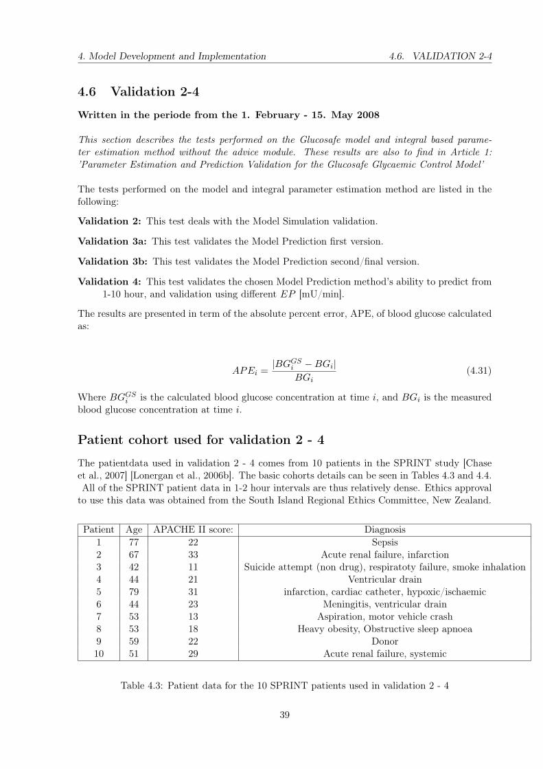
The patientdata used in validation 2 - 4 comes from 10 patients in the SPRINT study [Chaseet al., 2007] [Lonergan et al., 2006b]. The basic cohorts details can be seen in Tables 4.3 and 4.4.All of the SPRINT patient data in 1-2 hour intervals are thus relatively dense. Ethics approval

to use this data was obtained from the South Island Regional Ethics Committee, New Zealand.

Patient Age APACHE II score: Diagnosis1 77 22 Sepsis2 67 33 Acute renal failure, infarction3 42 11 Suicide attempt (non drug), respiratoty failure, smoke inhalation4 44 21 Ventricular drain5 79 31 infarction, cardiac catheter, hypoxic/ischaemic6 44 23 Meningitis, ventricular drain7 53 13 Aspiration, motor vehicle crash8 53 18 Heavy obesity, Obstructive sleep apnoea9 59 22 Donor10 51 29 Acute renal failure, systemic

Table 4.3: Patient data for the 10 SPRINT patients used in validation 2 - 4

39

4.6. VALIDATION 2-4 4. Model Development and Implementation

Patient Length of stay in hospital (hours) Length of stay on SPRINT (hours) Gender Diabetes1 580.8 312 M No2 458.4 162 M No3 408 253 M No4 223.2 207 F No5 55.2 39 F No6 280.8 161 F No7 861.6 17 M No8 477.6 182 M No9 99.6 93 F No10 520.8 360 M No

Table 4.4: Length of stay and further patient data for the 10 SPRINT patients used in Validation2 - 4.

40


Validation 2

This test documents the Model Simulation validation, which also is presented in the article ’Pa-rameter Estimation and Prediction Validation for the Glucosafe Glycaemic Control Model’.The Model Simulation process finds a patient specific SI (= SI1,...,SIi,...,SIN ) profile over time

Figure 4.18: Flowchart over the work process for the Model Simulation Validation. First the model simulatesand finds the entire SI profile for a patient at once. Thereafter the model repeats the same simulation using thefounded SI profile from the first simulation.

for a given set of patient data (glucose measurements BGi and insulin and nutrition interven-tions, IV).When a new blood glucose measurement BGi becomes available at time ti a new value SIi canbe identified from the measurements BGi−1 and BGi.In the Model Simulation mode, Glucosafe can use SIi to simulate BGi, using BGi−1 as the initialvalue for the simulation:

BGGSi = GS(BGi−1, SIi; IV )

where BGGSi is the simulated blood glucose at time ti using SIi and the interventions IV starting

from time ti−1 with the measured blood glucose value BGi−1.A close match between BGGS

i and BGi will confirm that the identified patient profile SI actuallydescribes the dynamics of the patients metabolic state (APEi).Figure 4.19 illustrates the results for Patient 4 in the Model Simulation validation. In Ap-pendix A.4 on page 83, Article 1 first edition, more of these Model Simulation validation can

41


be seen. Dots with error bars show measured clinical data and the line is the identified model.The overall fits are qualitatively very good. The second panel shows the SI profile. The fitteddata error results for the Model Simulation validation for all 10 SPRINT patients are presentedin Table 4.5. Table 4.5 shows mean and median APE’s per patient over the cohort are 0.45 and0.24 % and 100 % of measurements per patient being less than 10 % APE.

Figure 4.19: Model Simulation validation of Patient 4. Panel 1 shows the simulated blood glucose, meanwhilethe dots are the measured blood glucose. Panel 2 is the calculated plasma and peripheral plasma concentration.Panel 3 is the given nutrition, and Panel 4 is the given insulin. Finally, panel 5 is the SI identified in simulationmode (identified in Model Simulation, see Figure 4.18 on the preceding page). The entire data set is fit as a whole.

42


SPRINT Number of Mean Median IQR 5-95% Percent APEi

patient simulations Range < 10%1 234 0.50 0.18 [0.07 0.45] [0.01 1.32] 1002 154 0.34 0.23 [0.08 0.46] [0.01 1.07] 1003 170 0.56 0.38 [0.18 0.69] [0.02 1.62] 1004 192 0.49 0.29 [0.14 0.57] [0.02 1.59] 1005 32 0.72 0.51 [0.18 0.98] [0.05 2.72] 1006 112 0.53 0.30 [0.12 0.64] [0.03 2.17] 1007 12 0.84 0.29 [0.12 0.63] [0.02 2.61] 1008 114 0.60 0.23 [0.12 0.55] [0.03 1.65] 1009 83 0.51 0.35 [0.16 0.55] [0.05 1.71] 10010 252 0.34 0.20 [0.07 0.42] [0.02 1.05] 100

Overall 1355 0.45 0.24 [0.10 0.51] [0.01 1.33] 100

Table 4.5: Results for the Model Simulation validation of Glucosafe of all SPRINT patients invalidation 2. The Overall result is weighted by the amount of data for each patient. IQR =interquartile range.

Conclusion of Validation 2

The results of the validation presents a mean APE at 0.45 %. This result proves that the modeldynamic of Glucosafe during Model Simulation fits the measured blood glucose data within anacceptable error range, and ready for being used in Model Prediction..

43


Validation 3

The development of the Glucosafe model and the integral based parameter estimation methodhas been through several states of improvements.Due to fully document my work process, it is necessary to illustrate the two ways of ModelPredictions I have used during the development of the project.Figure 4.20 illustrates the two different Model Prediction methods, and therefore also two states

Figure 4.20: This figure illustrates the two Model Prediction methods, which have been used. The first predictionmethod is shown in the left column, meanwhile the second, and final Model Prediction method is presented in theright column

44


of development, to initiate Model Prediction.Both Model Prediction methods have the ability to identify the patient parameter SI to minimizethe APEi between BGGS

i which is the calculated blood glucose concentration at time i, and BGi

which is the measured blood glucose concentration at time i.The first Model Prediction method shown in the left column in Figure 4.20, presents the firstedition of the Model Prediction.The prove of need of always using a combined system utilizing both a model and a parameterestimator, can be seen by observing Figure 4.14 on page 33, where the result is presented of usingthe Glucosafe model alone, without the ability to estimate SI , but instead a fixed SI during thetotal simulation period. Figure 4.19 presents the combined system utilizing both the model andthe parameter estimator.Simply by observing these two figures, it is possible to see that the need of parameter estimatoris important.

The first Model Prediction method had a big disadvantage, due to the missing ability to predictSI in realtime.Model Prediction method working in realtime became necessary, when the system had to beused against a patient, whose data also becomes accessible en realtime depending on a real bloodglucose measurement device, or virtual patients with unknown interventions - In other word itbecame necessary if the current system should work as a part of a glycaemic control system.

After developing the second, and final edition of the Model Prediction method, presented inthe right column in Figure 4.20, the ability to predict in realtime was achieved.To fully document both Model Prediction methods, these are both validated:

Validation 3a: Validation of the first Model Prediction method. The full result of this methodis presented in Appendix A.4 on page 83, which includes the first edition of the article Pa-rameter Estimation and Prediction Validation for the Glucosafe Glycaemic Control Model.

Validation 3b: Validation of the second, and final Model Prediction method. This method islater used in the development of the Decision Support System, using the Advice Module.

The results of this validation is presented in Article 2.

45


Validation 3a

This test validates the first Model Prediction method, which is shown in the left column inFigure 4.20 on page 44.Visuel results for Validation 3a can be seen in Appendix A.4 on page 83, where Article1oldpresents this. The results for the first Model Prediction method is done as illustrated in the leftcolumn in Figure 4.20 on page 44.The results for the Model Prediction validation for all 10 SPRINT patients included in this testis presented in Table 4.6.

46


SPRINT Number of Mean Median IQR 5-95% APE Percent of measurementspatient Predictions (APE) (APE) Range < 10% APE

1 234 11.58 9.51 [4.83 15.08] [0.58 29.50] 53.022 154 11.32 8.12 [3.46 17.69] [0.50 29.50] 54.613 170 18.12 14.31 [6.89 27.36] [0.56 41.93] 36.904 192 10.73 7.46 [3.37 13.93] [0.58 34.60] 60.005 32 15.35 13.02 [7.19 22.57] [0.71 38.73] 36.676 112 9.26 5.89 [2.56 11.97] [0.34 29.07] 71.817 12 14.65 13.73 [11.90 17.72] [6.76 18.20] 18.188 114 16.28 11.50 [5.83 19.78] [1.35 47.49] 40.189 83 15.81 12.50 [5.95 18.65] [1.25 44.41] 41.9810 252 12.58 9.93 [4.43 17.58] [0.79 31.95] 50.4

Overall 1355 13.02 9.91 [4.74 17.78] [0.75 34.75] 50.78

Table 4.6: Results for Model Prediction validation (3a) with integral parameter estimation ofall SPRINT patients in this test. The Overall result is weighted by the amount of data for eachpatient. IQR = interquartile range

47


Validation 3b

The results for the Model Prediction validation for all 10 SPRINT patients included in this testis presented in Table 4.7.Figure 4.6 illustrates the results for Patient 8 in the Model Prediction validation 3b. Dots witherror bars show measured clinical data and the line is the identified model. The overall fits arequalitatively very good.

Figure 4.21: Model Prediction validation of Patient 8. Panel 1 shows the predicted blood glucose, meanwhile thedots are the measured blood glucose. Panel 2 is the calculated plasma and peripheral plasma concentration. Panel3 is the given nutrition, and Panel 4 is the given insulin. Finally, panel 5 is the SI identified during prediction.The data seen are fitted hour to hour as seen in the right column in Figure 4.20

48


SPRINT Number of Mean Median IQR 5-95% APE Percent of predictionpatient Predictions (APE) (APE) Range measurements < 10% APE

1 234 9.7 7.1 [3.6 13.0] [1.6 25.7] 66.52 154 9.9 7.5 [3.9 13.4] [1.5 25.3] 61.83 170 12.3 10.6 [3.9 18.6] [1.5 30.6] 48.14 192 11.2 7.9 [3.7 12.1] [1.7 32.2] 62.85 32 14.8 14.3 [6.5 20.4] [2.3 35.8] 33.36 112 9.1 6.1 [3.2 12.5] [0.8 32.6] 69.77 12 13.4 8.5 [3.8 15.1] [2.4 30.9] 54.58 114 11.2 7.1 [4.5 12.6] [0.6 37.3] 63.69 83 16.4 12.3 [7.0 19.6] [1.6 36.8] 41.010 252 9.3 6.3 [3.4 11.8] [0.8 24.5] 67.3

Overall 1355 10.8 8.0 [4.0 13.9] [1.2 29.5] 60.9

Table 4.7: Results for Model Prediction validation (3b) with integral parameter estimation of allSPRINT patients in this study. All results are shown in percent. The Overall result is weightedby the amount of data for each patient. IQR = interquartile range

Conclusion of Validation 3a + 3b

The test results for validation 3a presents a mean APE at 13.02 and a median APE at 9.91. Thetest results for validation 3a presents a mean APE at 10.8 and a median APE at 8.0.Only Validation 3b present a acceptable low Model Prediction error, as compared to the Glu-cometers used at Christchurch Hospitals with 7-12 % measurement error [Hann et al., 2005].The results for validation 3a have a bigger APE than the results presented in validation 3b, thepreferred method is therefore the Model Prediction tested in validation 3b.The reason for the difference in predictions errors (APE) between Validations 3b and 3a, is thatthe Model Prediction method validated in 3b handles sudden big changes in a patients bloodglucose [mmol/L] better than 3a.Besides the better prediction error, the Model Prediction tested in validation 3b is the onlymethod estimating SI in realtime, see the right column in Figure 4.20 on page 44, and thereforethe only method that can be used in a glycaemic control system with unknown future interven-tions.Hence, in the chosen Model Prediction mode (3b), SIi is used to simulate the next measurement,BGi+1, using BGi as the initial value for the simulation:

BGBGi+1 = GS(BGi, SIi; IV )

A close match between BGBGi+1 and BGi+1 shows that the identification of SI can provide an

accurate prediction of the response to clinical intervention.

A more comprehensive documentation of the results achieved in validation 3b can be seen inArticle 1.

49


Validation 4

This test validates the chosen Model Prediction methods ability (3b) to predict from 1-10 hour,see Figure 4.22, and testing the prediction errors (1 hour predictions only) using different EPvalues, see Figure 4.23 on the facing page.

The Model Prediction validated in validation 3 has used a fixed EP at 27.77 mU/min. Due

Figure 4.22: This figure illustrates the systems ability to predict over a period up to ten hours for the close-to-average Patient 6 in the study, using different EP values. The result for this capability is presented using the unitRoot Mean Square of the Relative Logarithmic Error.

to minimize the model Prediction error APE, different values of EP has been tested.Figure 4.23 on the next page illustrates that the parameters EP and SI are interdependent inthe model as it is defined. A change in EP therefore changes the patients SI profile over thepatient.It also shows how EP and SI are dependent and trade off for Patient 6. As EP increases SI

falls and vice versa, with similar dynamics in the SI profiles.

50


Figure 4.24 on the following page illustrates the relationship between choice of EP and resultingoverall median APE for all 10 patients. The overall median APE for model Prediction has beentestet for choices of EP at 20, 27.77, 30, 35, 40 and 45 mU/min. The dots in Figure 4.24 theModel Prediction result (overall median) for all 10 patients, and the best overall choice for EPto have, is a EP value at 27.77 mU/min. However, using a EP value at 27.77 mU/min maynot be the optimum solution in other situations, with another/lesser critically ill patient cohort(higher SI).

Figure 4.23: This figure illustrates how the predicted blood glucose for Patient 6 is effectively the same by usingdifferent dependent set of EP and SI profiles. The top picture shows 3 predictions produced by using 3 differentEP and SI profiles. The lower picture shows 3 different SI profiles. The upper SI profile is produced by using aEP = 27.77 mU/min and the lower SI profile is produced by using a EP = 45 mU/min. The prediction lines inthe top panel are close to be the same. This figure is produced by 1 hour prediction only.

51


Figure 4.24: This figure illustrates the overall median error (APE) for all 10 patients used in this study, usinga different value of EP.

Conclusion of Validation 4

The tested Model Prediction method has shown to be acceptable for later use in a control scenariowith unknown interventions. Furthermore, the Model Prediction are considered acceptable forlater use in control applications in a clinical setting out to approximately 3 hour predictionslevels, as see in Figure 4.22. These results validate using these models in proof of concept pilotclinical trials and the later development of a advice module to complete the study. The fixed EPvalue at 27.77 mU/min are found to be the optimum value for the tested cohort, and are usedin the later development of the system.

52

Chapter 5

Advice Module Development andImplementation

5.1 Advice module

Written in the periode from Thursday the 7. May - 2. June 2008

In this section the advice module of the glycaemic control system is being defined and described.This part of my work is also presented in Article 2: ’Development and Validation of a DecisionSupport System for Critically Ill Patients utilizing the Glucosafe Glycaemic Control Model’.

The development of the advice module, in the glycaemic control system, depends on the pres-ence of the earlier implemented Glucosafe model, see section 4.2 on page 15, and integral basedparameter estimation method, described in section 4.5 on page 35. The development and imple-mentation of the Glucosafe model and the integral based parameter estimation method, mainlyrepresents my work done in the first half of this study.

Figure 5.1 on the next page illustrates the build up of the full glycaemic control system, whichincludes the model, integral based parameter estimation method, advice module (all in the rightcolumn in the figure) and a patient - which in this study is a virtual patient (left column in thefigure). This chapter will focus on the development of the advice module, and the virtual patientneeded for validation of the glycaemic control system.

The included parts of the advice module are presented in the following:

Blood glucose penalty function: The purpose of the glycaemic control system is to keep thepatient normoglycaemic, and therefore is the blood glucose penalty function designed togive a high penalty when a set of intervention can cause that the patients blood glucosegets outside the normoglycaemic range.

Nutrition penalty function: Even though the main purpose of the glycaemic control systemis to maintain a state of normoglycaemia, the patient also has to have a certain amountof calories during the glycaemic control. The glycaemic control is because of the nutritionpenalty function, a compromise between always being normoglycaemic and getting optimalfeeding.

Insulin penalty function: The purpose of this penalty function is to give a high penalty when

53

5.1. ADVICE MODULE 5. Advice Module Development and Implementation

Figure 5.1: This figure illustrates the full glycaemic control system, which includes the model, integral basedparameter estimation method, advice module and a virtual patient. Further explanation of the nutrition andinsulin advices can be seen in the sections of penalty functions and the advice module optimizer

a high amount of insulin is given, due to stay in control of the patients blood glucoseconcentration.

Advice module optimizer: The given sets of interventions are a result of the advice moduleoptimizer, which uses the three mentioned penalty functions to find the lowest possiblesum of penalty to chose the optimum sets of nutrition and insulin to give to the patient.

Next, each of the listed parts of the advice module, followed by the virtual patients are explainedin terms of concept and implementation.

Blood glucose penalty function

In addition to the Glucosafe glucose-insulin system model and integral based parameter estima-tion method, the glycaemic control system utilizes three penalty functions and an optimizer, dueto the control of the blood glucose concentration of patients.

54

5. Advice Module Development and Implementation 5.1. ADVICE MODULE

All three shapes have influence on glycaemic control, and the size or values of each penaltyfunction are weighted against the desired criteria of 1: keeping the patients blood glucose con-centration inside the normoglycaemia range between 4.4-7.75 mmol/L [Van den Berghe et al.,2001] [Krinsley, 2004]. 2: giving the patient an adequate amount of calories, and 3: keepingthe control of the patients blood glucose concentration while minimizing the amounts of insulingiven to the patient.

The approach of design of the penalty functions, has in this study been the blood glucose penaltyshape, see Figure 5.2, with basis in previous work [Andreassen et al., 1994]:

BGpenalty = (ln(BG

BG0))2 ×KBG−Penalty (5.1)

where BG is the current blood glucose values, and BG0 (= 5.5 mmol/L) is the point at whichthe penalty function value is 0. KBG−Penalty is a fitting constant (value = 4). The blood glucosepenalty function results in a penalty range between: [0 0.47] in the targeted blood glucose rangeof 4.4-7.75 mmol/L.

Figure 5.2: This figure illustrates the shape of the blood glucose penalty function

55


Nutrition penalty function

The nutrition penalty function, illustrated in Figure 5.3 on the next page, is designed on thebasis of keeping the patient normoglycaemic while continually giving the patient as close to 100% of daily intake (DI) as possible. The penalty range for the nutrition penalty function is [0.000.05] in the feeding range between 40-140 % of DI. Equation 5.2 represents the nutrition penaltyfunction:

Penalty(NUT ) = (NUT − 100%)2 ×KNUT−Penalty (5.2)

where NUT is given nutrition in the range 40-140 % of DI and KNUT−Penalty is a fitting con-stant (value = 0.15) to weight the nutrition penalty range against the two other penalty functions.

The nutrition advice range illustrated in Figure 5.3 is presented in % of DI, and has to beconverted into caloric intake for the specific patient. The Harris Benedict metabolism equation[Harris and Benedict, 1918] is used to calculate 100 % of daily calorie intake DI from the patientsgender, weight, age and height, from which calories per day (CD) can be calculated as: CD =NUT × DI [kcal/day]. The Harris Benedict metabolism equation is presented in the following,where CD in Equation 5.3 is full daily calorie need for men [kcal/day], and CD in Equation 5.4is full daily calorie need for women [kcal/day]:

CD = 66.5 + 13.8× weigth + 5× height− 6.8× age (5.3)

CD = 655.1 + 9.6× weigth + 1.8× height− 4.7× age (5.4)

where weight is in [kg], height in [cm] and age in [years] [Harris and Benedict, 1918].Finally, the advised feeding rate (FR) [ml/h] can be calculated as FR = CD/CV from the calorievalue CV [kcal/ml] of the enteral or parenteral solution. Additionally, see Appendix A.2 onpage 80 for documentation of CV and nutrition type given to the SPRINT cohort.The nutrition used in this study is an enteral formula named Diabetic Resource (Novartis MedicalNutrition, Minneapolis, MN, USA), which was also used in earlier studies from which the under-lying SPRINT patient data for the virtual patients in this study originates [Chase et al., 2008b][Chase et al., 2007] [Lonergan et al., 2006a] [Chase et al., 2008a] [Lonergan et al., 2006b]. Impor-tantly it is also a low carbohydrate formula, where 34 % of the calories come from carbohydrates.

The design criteria for limiting the nutrition to 40-140 % of DI, is that there is no need forexcessive nutrition feeding, due to the cause of or exacerbating hyperglycaemia [Patino et al.,1999]. The lower limit of 40 % of DI is set as the minimum possible calorie intake for patientswithout increasing mortality [Krishnan et al., 2003].

56


Figure 5.3: This figure illustrates the shape of the nutrition penalty function

Insulin penalty function

The insulin penalty shape is based on the saturation effect of insulin action on glucose uptake[Rizza et al., 1981] [Katz et al., 1993]. The shape for the insulin penalty function is illustratedin Figure 5.4 on the next page.Saturation has effect when calculating the nonlinear fraction of maximal endogenous balance asa function of the insulin infusion/absorption rate.The calculation of the insulin penalty functions is presented in Equation 5.5 and 5.6:

Penalty(INS) = ((I + Km)2

(Km)2− 1)×KINS−Penalty (5.5)

where Km is the insulin saturation constant (value = 28 mU/L) [Andreassen et al., 2008] andKINS−Penalty is a insulin penalty function fitting constant (value = 1/280).Finally, I [mU/L] depends on the insulin bolus given [U/h] defined in Equation 5.6:

I = INS × C ×BM70 (5.6)

where INS is the insulin bolus from 0-6 U/h (presented as P (t) in Figure 4.3 on page 16), andC is the default conversion factor (value = 98.1 [kg × min/L]) [Pielmeier et al., 2008] to convertabsorbed insulin to plasma insulin, and BM70 is a bodymass constant (value = 1/70 kg−1).The system limits the insulin bolus range to 0-6 U/h, and to minimize saturation effects theinsulin penalty range is [0 0.13]. The constant KINS−Penalty in Equation 5.5 is thus a fitting

57


constant, whose purpose is to weight the insulin penalty range against the two other penaltyfunctions.

Figure 5.4: This figure illustrates the shape of the insulin penalty function

Advice module optimizer

As seen on Figure 5.5 on page 60 the advice module optimizer uses all three penalty func-tions (Penalty(INS), Penalty(NUT ) and Penalty(BG)), and forward simulates the model(simulation(INS,NUT )) every intervention interval to choose the advice choice with the lowestsum of penalty error (Advice = min(Total Penalty(INS,NUT))).

In the top of the figure an array of different combinations of given insulin (INS) and givennutrition (NUT ) can be seen. The optimizer searches this grid of choices before every new in-tervention advice is given to the virtual patient. The optimizer calculates the penalty for eachof 7 possible insulin combinations (0-6 U/h). Meanwhile, the nutrition to be given is calculatedfor each possible combination over the range: 40, 60, 80, 100, 120, 140 % of DI. This search thusresults in 7 × 6 = 42 sets of possible interventions, and therefore 42 times where the optimizerforward simulates how the blood glucose concentration will respond to each different set of in-terventions.

58


As seen on Figure 5.5 each field of the grid involves a simulation for 3 hours, using the same setof interventions and SI for the three hour period. The result from this simulation is the set ofblood glucose concentrations: bg60, bg120 and bg180, which are the blood glucose concentrationsafter 1,2 and 3 hours, respectively. As seen in Figure 5.5 each set of possible interventions includethe blood glucose penalty sum over 3 hours (Equation 5.7), achieved from the simulation:

BGsum = Penalty(bg60) + Penalty(bg120) + Penalty(bg180) (5.7)

At each field in the grid, having a set of insulin and nutrition, and the resulting development inthe calculated blood glucose concentration (bg60, bg120 and bg180), these values are used as inputsto the penalty functions to find a penalty sum. The resulting advice is given after repeating thismethod for each field in the grid (42 times), and yields the combination with the lowest sum ofpenalties.

The functionality and success of the advice module controller depends on that there alwaysonly is given one advice (Advice = min(Total Penalty(INS,NUT))), by meaning that the advicemodule controller chooses only one minimum of sum of penalty.The chance of the advice module optimizer chooses more than one advice is very little, especiallybecause of the amount of digits involved in each penalty functions calculations. Also, is the finalglycaemic validation involving all 20 virtual patients, described in Article 2, done successfullywith the risk of having two advices.Conclusively, the risk of a advice module controller breakdown due to the calculation of an adviceresults in more than one advice, is theoretical.Even though, to ensure the glycaemic control systems stability on larger cohorts, a solution isnecessary, which is implemented into the advice module controller in form of two catches anddescribed in the following:

• Catch 1: In case of two or more global minimums in the calculation: (Advice = min(TotalPenalty(INS,NUT))), then choose the result which will give the smallest blood glucosepenalty BGsum for the blood glucose concentrations (bg60, bg120 and bg180).

• Catch 2: In case Catch 1 results in more than one solution, then choose the advice, whichwill result in the lowest nutrition penalty.

59


Figure 5.5: This figure illustrates how the advice module optimizer calculates all relevant combinations of nutri-tion and insulin in a grid to choose the advice choice with the lowest sum of penalty. During each 3 hours penaltysimulation, the same SI estimated for that hour is used.

Design of virtual patient

All retrospective data and measurements are available in 1-2 hour intervals, and are thus rel-atively dense. Ethics approval to use this data was obtained from the South Island RegionalEthics Committee, New Zealand.

As seen in the left column in Figure 5.1 on page 54 this study’s concept of a virtual patient,is the blood glucose response using the Glucosafe model for a model simulation. This virtualpatient simulation utilizes a previously generated SI profile, which original comes from 20 criticalcare patients also used in an earlier study with a specific SPRINT cohort [Chase et al., 2007][Lonergan et al., 2006a] [Lonergan et al., 2006b], also see Appendix A.2 on page 80. The generalcriteria for the Benchmark dataset is that the entry blood glucose concentration is higher than8 mmol/L, and all 20 patients have been on SPRINT for at least 5 days [Chase et al., 2008a].To imitate a blood glucose measurement on a real patient, noise is added to the virtual patients

60


Patient Age APACHE Diagnosis Hospital Duration of stay Gendernumber II stay (hours) on

score: SPRINT (hours)1 75 17 Hypoxemic 1416 828 M2 68 18 On pump 439 178 M3 73 22 Perforation 391 310 M4 68 19 Laparotomy 185 145 M5 60 13 Chronic obstructive airways disease 254 205 F6 70 31 Community acquired pneumonia 648 512 M7 70 42 Obstruction 770 159 F8 65 25 Septic shock 298 287 F9 76 20 Acute abdominal aortic aneurysm 511 458 F10 58 15 Hip replacement 142 139 F11 49 30 Hypoglycaemia 302 297 M12 73 16 Pancreatitis 156 150 M13 20 15 Trauma 1178 971 M14 74 23 Infarction/ischaemia 230 192 M15 63 29 Ventilatory 770 323 F16 49 14 Pancreatitis 929 923 M17 45 16 Pancreatitis 653 524 M18 72 16 Post op. 295 265 M19 73 22 Orthopaedic 257 253 M20 65 7 Community acquired pneumonia 149 140 F

Table 5.1: Patient data for the 20 SPRINT patients used to validate the advice module. Noneof the involved patients have any type of diabetes

blood glucose response. The noise added is done as in Equation 5.8:

BGvirtual = BGsimulation + BGsimulation ×Normalµ,STD (5.8)

Where the BGsimulation is the virtual patients blood glucose response, in terms of a model sim-ulation with a duration of 1 hour. BGsimulation is added normal distributed noise with a meanvalue (µ) at 0 and a standard deviation (STD) at 0.10×BGsimulation.

The patient cohorts details used to the advice validation can be seen in Table 5.1.

61

5.2. VALIDATION 5 5. Advice Module Development and Implementation

5.2 Validation 5


In this section the advice module of the glycaemic control system is being validated. This sectiononly contains the preliminary validation of the system, meanwhile the final tests and statistics arepresented in Article 2: ’Development and Validation of a Decision Support System for CriticallyIll Patients utilizing the Glucosafe Glycaemic Control Model’.This validations main focus is to test the advice module, hence, is this also a test of the entireglycaemic glucose system, due to the results from this validation also reflects the Glucosafe model(see dedicated test for this part starting in section 4.6 on page 39) and integral based parameterestimation method (see section 4.5 on page 35 for dedicated test of this part).

The advice module preliminary validations included in Validation 5 covers the following:

• Validation of the glycaemic control systems ability to lower a patients blood glucose con-centration [mmol/L], when the patients blood glucose concentration is hyperglycaemic (inthis test a starting blood glucose concentration at 26 mmol/L). Furthermore, this is also atest of how long time it takes to achieve normoglycaemia (4.4-7.75 mmol/L).

• Validation of the glycaemic control systems ability to rise a patients blood glucose concen-tration [mmol/L], when the patients blood glucose concentration is hypoglycaemic (below2.2 mmol/L). Furthermore, this is also a test of how long time it takes to achieve normo-glycaemia (4.4-7.75 mmol/L).

• Validation of the glycaemic control systems ability to keep at patients blood glucose con-centration normoglycaemic (4.4-7.75 mmol/L) when the patients state of health is normalwith a insulin sensivity, SI equal to 1.

In Figure 5.6 the implementation of virtual patients can be seen. During a glycaemic control ofa given virtual patient, a predefined SI value is given to the virtual patient each hour, and noiseis added (like Equation 5.8 on the previous page) to the virtual patients blood glucose response,to the current intervention, to imitate a clinical situation with measurement noise. In this study,a normal distributed noise with a standard deviation of 10 % of the measured blood glucoseis used matching the glucometers used in the SPRINT study Chase et al. [2008b]. All listedvalidation of the glycaemic control system are done using the same starting criteria: plasmainsulin concentration at 20 mU/L and a peripheral insulin concentration at 12 mU/L. In thefirst two validations the virtual patient utilizes the underlying SI profile from Patient 1, listedin Table 5.1.For the two first preliminary validations included in this section Patient 1’s SI profile are loadedinto the virtual patient every hour to give the virtual patient a hour to hour changeable insulinsensivity profile (SI,i). After having calculated SIestimated(i+1), the advice module, comes upwith the new set of intervention to the virtual patient in the following hour (Nutritioni+1 andInsulini+1), see Figure 5.6.

62

5. Advice Module Development and Implementation 5.2. VALIDATION 5

Figure 5.6: This figure illustrates the dynamics of the glycaemic control system working on a virtual patientimitating a clinical scenario with blood glucose measurement noise

63


Advice Module Validation for patient coming from hyperglycaemia

Figure 5.7 illustrates the result for a hyperglycaemic patient (in this case a starting blood glucoseconcentration on 26 mmol/L) coming under glycaemic control. At hour 1 the first advice iscalculated to be used for the time interval between hour 1 and hour 2: 4 U/h insulin and 60 % ofDI nutrition is given to lower the blood glucose concentration [mmol/L]. At hour 4 the glycaemiccontrol system has achieved normoglycaemia for the patient (4.4-7.75 mmol/L).

Figure 5.7: This figure illustrates a hyperglycaemic patient coming on glycaemic control. The starting gut content2 mmol/kg, which result in a decreasing absorption rate [mmol/kg/min] in the start because of the low nutritionfeeding rate. The given SI profile originates from Patient 1 described in Table 5.1

64


Advice Module Validation for patient coming from hypoglycaemia

Figure 5.8 illustrates the result for a hypoglycaemic patient (the starting point for the bloodglucose concentration is 2.2 mmol/L) coming under glycaemic control. At hour 1 the first adviceis calculated to be used for the time interval between hour 1 and hour 2: 0 U/h insulin and 120% of DI nutrition is given to rise the blood glucose concentration mmol/L. After two hours ofcontrol, at hour 3, the glycaemic control system has achieved normoglycaemia for the patient(4.4-7.75 mmol/L).

At hour 1 the glycaemic control system chooses to give the patient 120 % of DI instead of140 % of DI, even though the patients is hypoglycaemic. The reason for this is that the absorp-tion rate [mmol/kg/min] responds slowly, representing in that the difference in nutrition penaltybetween 120 and 140 % of DI is bigger than the penalty difference of the two resulting bloodglucose concentrations (BGsum).

65


Figure 5.8: This figure illustrates a hypoglycaemic patient coming on glycaemic control. The starting gut content0.5 [mmol/kg], which result in a increasing absorption rate [mmol/kg/min] because of the high nutrition feedingrate. The given SI profile originates from Patient 1 described in Table 5.1

66


Advice Module Validation for healthy patient

Figure 5.9 illustrates the result for a healthy patient coming on glycaemic control. The aim ofthis validation is to shown that the glycaemic control system can keep a patients blood glucoseconcentration normoglycaemic (4.4-7.75 mmol/L) even though the patients insulin sensivity is1, and therefore differs a lot from the cohort used in this study, see Table 5.1.Like in the two previous validation the advice calculation begins at hour 1. The starting bloodglucose value in this validation is hyperglycaemic at 26 mmol/L, the goal is to keep and get thepatient inside the 4.4-7.75 mmol/L range.Overall during this validation, the nutrition feeding rate was close to 100 % of DI.

Figure 5.9: This figure illustrates a healthy patient coming on glycaemic control. The starting gut content is 2[mmol/kg]. The given SI profile is made up and set as a constant to imitate a healthy patient.

67


Conclusion to advice module preliminary validations

Through all 3 validations the Glycaemic control system succeeded in getting the patient into thenormoglycaemic range (4.4-7.75 mmol/L), and keeping the patient there.For the hyperglycaemic patient it took 4 hours, or 3 advice calculated interventions to achievenormoglycaemia. For the hypoglycaemic patient it took 3 hours, or 2 advice calculated interven-tions to achieve normoglycaemia. The validation with the healthy patient also proved that theglycaemic control system can keep the patient normoglycaemic.

From these preliminary validations of the advice module, the glycaemic control system is readyto be tested on a bigger scaled patient cohort, described in Table 5.1. The Validation of these20 critical care patients are presented in Article 2: ’Development and Validation of a DecisionSupport System for Critically Ill Patients utilizing the Glucosafe Glycaemic Control Model’.

68

Chapter 6

Evaluation

6.1 Discussion


In this section the full discussion of the project is presented by meaning that this discussion in-cludes both the topics of the Model Prediction design and result and the final design and results ofthe glycaemic control system. This discussion is consistent to both discussions in Article 1 and 2.

The Glucosafe model presented is physiologically defined and utilizes the concept of a remotecompartment for insulin transport to account for the delay between insulin secretion, or infusion,and utilization.The integral based fitting method proves effective in reducing a typically non-linear optimiza-tion problem to a linear, rapidly solved convex optimization problem. Overall, the fitted modelmatches all observed clinical dynamics, as seen in Table 4.7 in validation 3b and does so haveminimal error. These fitting results indicate that the model possesses all necessary mathematicaldynamics.The low Model Prediction error of Table 4.7 (and presented in Article 1), as compared to theGlucometers used at Christchurch Hospitals with 7-12 % measurement error [Hann et al., 2005],helps to further justify this choice of approach.

The system prediction model estimates only one parameter SI . As a result, the endogenousinsulin production (EP ) is kept constant. However, this assumption only shifts the identified SI

value if examined in a parametric study. Fitting both parameters in this model is problematic,as they are not uniquely identifiable without measured insulin data, which is rarely available incritical care. An added argument for only using SI as a variable parameter is that little is knownabout the kinetics of EP secretion, both in magnitude or variation over time, in the critically ill.

The parameters EP and SI are thus dependent and a change in EP therefore mostly scalesthe SI profile by a given value over the patient. Figure 4.23 on page 51 shows how 2 differentvalues for EP and the same SI profile scales the predicted blood glucose values for Patient 6 (inModel Prediction validation). The shifted dynamics for the three different cases are otherwiseclose to the same. It also shows how EP and SI are dependent and trade off for Patient 6. AsEP increases, SI falls and vice versa, with similar dynamics in the SI profiles.The Glucosafe model validated in this study has used a fixed EP at 27.77 mU/min. Due tominimize the model Prediction error APE, different values of EP has been tested.

69

6.1. DISCUSSION 6. Evaluation

Figure 4.24 on page 52 illustrates the relationship between choice of EP and resulting overallmedian APE for all 10 patients.The overall median APE for model Prediction has been tested for choices of EP at 20, 27.77,30, 35, 40 and 45 mU/min. The dots in Figure 4.24 on page 52 represents the Model Predictionresult for all 10 patients, and the best overall choice for EP to have, is a EP value at 27.77mU/min. However, using a EP value at 27.77 mU/min may not be the optimum solution inother situations, with a less critically ill patient cohort (higher SI).In general, the 1-hour prediction validation errors are relatively low and consistent. The cumu-lative distribution figure presented in Article 1 shows that 90 percent of the Model Predictionresults are below 25 % APE, and 60 percent are below 10 % APE. The same figure also shows anerror distribution that is clearly not normal. Hence, this study reports median and IQR valuesto better represent the data than normal statistics.

The Glucosafe model used in this glycaemic control system presented, is physiologically de-fined and utilizes the concept of a remote compartment for insulin transport to account for thedelay between insulin secretion, or infusion, and its utilization. A prior validation shows thatthe fitted model matches all observed clinical dynamics [Lotz, 2007] [Pielmeier et al., 2008]. Thisverifies the use of blood glucose response of virtual patients, who are constructed using the samemodel added noise, to be the single scale of which the validation of the glycaemic control systemis tested against.

In terms of the design of the advice module in the glycaemic control system where the resultsshowed in section 5.2 on page 62 that there is a need to adjust the nutrition and insulin given,to keep the patient inside the normoglycaemia range (4.4-7.75 mmol/L).The results of glycaemic control validation (presented in Article 2), regarding the average nu-trition rate, and the ability to keep the patients inside the range of normoglycaemia, are goodexamined in isolation. However, more importantly, in combination the compromise betweennutrition given (87.17 % of DI), and the ability to keep patients normoglycaemic (87.73 % ofmeasurements), can be hard to achieve with this general ICU cohort.The overall normal average calorie intake per day was 1250 kcal/day, and the overall averagegiven insulin was 2.2 U/h, which makes the results from this study comparable to other similarstudies - for example the SPRINT clinical implementation and evaluation study by Chase etal. [Chase et al., 2008b], where the overall lognormal average calorie intake per day were 1283kcal/day and overall average given insulin per hour were 2.8 U/hour.

In a later clinical scenarios, there are potential limitations in the advices of the glycaemic control.Some hospitals use fixed nutrition feeding rates (fx. 100 % of DI), so that insulin [U/h] is the onlyadjustable parameter ensure patients are kept normoglycaemic. Observing Table II in Article 2it can be seen that most of the average feeding rates for all 20 patients are in the 80-100 range[% of DI], depending on the patients average SI . Hence, without modulating nutritional inputsmany similar general ICU patients will have periods of hyperglycaemia where insulin alone maynot be fully effective.

70

6. Evaluation 6.2. CONCLUSION

6.2 Conclusion


In this section the conclusion of the full project is presented regarding the topics of the ModelPrediction design, results and the final design and results of the glycaemic control system. Thisconclusion is consistent to both conclusions in Article 1 and 2.

This study examines and validates the Glucosafe glycaemic control model for critical care pa-tients in simulation using retrospective clinical data. The model is also validated for its predictiveability (also presented in Article 1). The Model Prediction utilizes an integral based parameterestimation method for fitting the patient specific insulin sensivity SI . The goal is to ensureprediction with minimal absolute percent error, and to assess the models potential clinical util-ity. The Model Prediction validation and examination (Validation 3b) used retrospective clinicaldata from glycaemically controlled critical care patients. The basic patient data for this cohortare presented in Tables 4.3 and 4.4.

The overall mean and median absolute percent error for both Model Simulation and ModelPrediction are within measurement error.Both results for Model Simulation validation (Validation 2) and Model Prediction validation(Validation 3b) are considered acceptable for later use in control applications in a clinical settingout to approximately 3 hour predictions levels, as seen in Validation 4. These results validateusing these models in proof of concept pilot clinical trials.Furthermore, this study presents and validates a glycaemic control system, utilizing the Glucosafemodel Pielmeier et al. [2008] and an integral based parameter estimation method for fitting thepatient specific insulin sensivity SI [Hann et al., 2005] (also presented in Article 2). The goalof the glycaemic control validation is to prove the glycaemic control systems ability to keep 20virtual patients (produced by patientdata using retrospective clinical data (SPRINT)) inside therange of normoglycaemia (4.4 - 7.75 mmol/L).

The overall median blood glucose concentration for all 20 patients in the glycaemic controlvalidation is 6.05 mmol/L, and the IQR is 5.54-6.62 mmol/L. The basic patient data for this co-hort are presented in Table 5.1. The overall number of hypoglycaemic measurements per patientis 0 (blood glucose measurements below 2.2 mmol/L). The overall mean percent of measurementsinside the normoglycaemic range (4.4-7.75 mmol/L) is 87.7 %.

Because of the low variation of average feeding given to the virtual patients, and that theoverall average feeding is very close to reach full calorie need, the glycaemic control system isconsidered comparable to other similar studies [Chase et al., 2008b], and acceptable for later usein control applications in a clinical setting using real patients.The results presented in this study validates using the current version of the glycaemic controlsystem in proof of concept pilot clinical trials.

71

6.3. FUTURE WORK 6. Evaluation

6.3 Future work


This section contains the aspects for future work of the results achieved during the period ofdeveloping the glycaemic control system. This section can be read together with the full overviewof the decision support system described in section 4.1 on page 12.

The current state of the glycaemic control system is its ability to keep virtual patients bloodglucose concentration normoglycaemic (4.4-7.75 mmol/L). These virtual patients are build uponreal patient data (SPRINT) [Chase et al., 2008b] [Chase et al., 2008a]. The next step of devel-oping of the glycaemic control system is to add a user friendly interface to medical staff at theICU, and by that make it a stand alone decision support system to help medical staff and realcritical ill patients, in terms of the nutrition feeding rate [ml/h] and given insulin [U/h] to thesepatients.The primary task of the decision support systems user interface should be to give insulin [U/h]and nutrition [ml/h] advices to the medical staff, and to be the systems input user interface, fromwhere the decision support system can receive the latest measured blood glucose measurement[mmol/L], of the patient under control, to update the model for continuing the glycaemic control.It is intended for the decision support system to work together with the local medical staff, andit should be possible for the staff to bypass the advice given from the system, and instead giveindependent nutrition and insulin advices. when that happens, the medical staff should informthe decision support system with the new intervention, so that the glycaemic control system canbe updated to continue as normal.Furthermore, different intensive care units can have different treatment politics, in terms of theinterventions given to the critical ill patients under glycaemic control. Therefore, the advicemodule optimizer shall have a build in functionality to work after the local rules of intervention:fx. always feed at a 100 % of DI, different insulin and nutrition limitations ([% of DI] and [U/h]).Finally, the decision support system’s imbedded physiological model, has to be upgraded to havean adaptive patient specific post-hepatic endogenous insulin production (EP ) functionality, dueto improve the advice given for each patient under glycaemic control.

72

6. Evaluation 6.3. FUTURE WORK

Figure 6.1: This figure shows the step from going from a glycaemic control system working on virtual patients,to be a decision support system working together with medical staff to optimize the treatment of real critical illpatients. The top part illustrates the dynamics of the glycaemic control system working on a virtual patientimitating a clinical scenario with blood glucose measurement noise, meanwhile the lower part gives an overview ofthe involved hardware in the system and the actors that the system has to work with when the glycaemic controlsystem is developed to work as a decision support system.

73

Bibliography

Andreassen, S., Benn, J. J., Hovorka, R., Olsen, K. G., and Carson, R. E. (1994). A probalisticapproach to glucose prediction and insulin dose adjustment: description of metabolic modeland pilot evaluation study. Computer Methods and Programs in Biomedicine, 41:153–165.

Andreassen, S., Pielmeier, U., and Chase, G. J. (2008). Receptorbased models of insulin satura-tion dynamics. Sixth IASTED International Conference on Biomedical Engineering. Innsbruck,Austria.

Arleth, T., Andreassen, S., Federici, M. O., and Benedetti, M. M. (2000). A model of theendogenous glucose balance incorporating the characteristics of glucose transporters. ComputerMethods and Programs in Biomedicine, 62(3):219–234.

Barsheshet, A., Garty, M., Grossman, E., Sandach, A., Lewis, B., and Gottlieb, S. (2006).Admission blood glucose level and mortality among hospitalised nondiabetic patients withheart failure. Archives of Internal Medicine, 166(15):1613–1619.

Capes, S., Hunt, D., Malmberg, K., and Gerstein, H. (2000). Stress hyperglycaemia and increasedrisk of death after myocardial infarction with and without diabetes: A systematic overview.Lancet, 355(9206):773–778.

Capes, S., Hunt, D., Malmberg, K., Pathak, P., and Gerstein, H. (2001). Stress hyperglycaemiaand prognosis of stroke in nondiabetic and diabetic patients: a systematic overview. Stroke,32(10):2426–2432.

Cauter, E. V., Mestrez, F., Sturis, J., and Polonsky, K. S. (1992). Estimation of insulin secretionrates from c-peptide levels. comparison of individual and standard kinetic parameters for c-peptide clearance. Diabetes, 41(3):368–377.

Chase, G. J., LeCompte, A., Shaw, G. M., Blakemore, A., Wong, J., Lin, J., and Hann, Christo-pher, E. (2008a). A benchmark data set for model-based glycemic control in critical care.Submitted (DST).

Chase, G. J., Shaw, G. M., LeCompte, A., Lonergan, T., Willacy, M., Wong, X., Lin, J., Lotz,T., Lee, D., and Hann, C. (2008b). Implementation and evaluation of the sprint protocolfor tight glycaemic control in critically ill patients: a clinical practice change. Critical Care,12:R49.

Chase, G. J., Shaw, G. M., Wong, X., Lotz, T., Lin, J., and Hann, C. E. (2006). Model-basedglycaemic control in critical care: A review of the state of the possible. Biomedical SignalProcessing & Control, 1:3–21.

Chase, J. G., Andreassen, S., Pielmeier, U., and Hann, C. E. (2008c). Glucose-insulin pharma-codynamic surface modeling comparison. IFAC World Congress - Biomedical Engineering.

74

BIBLIOGRAPHY BIBLIOGRAPHY

Chase, J. G., Shaw, G. M., Lotz, T., LeCompte, A., Wong, J., Lin, J., Lonergan, T., Willacy, M.,and Hann, C. E. (2007). Model-based insulin and nutrition administration for tight glycaemiccontrol in critical care. Current Drug Delivery, 4(4):283–296.

Chee, F., Fernando, T., and van Heerden, P. (2003). Closed-loop glucose control in critically illpatients using continuous glucose monitoring system (cgms) in real time. IEEE Trans. Inf.Technol. Biomed., 7(1):43–53.

Despopoulos, A. and Silbernagl, S. (1991). Color Atlas of Physiology. Thieme, 4 edition.

Hann, C. E., Chase, G. J., Lin, J., Lotz, T., Doran, C. V., and Shaw, G. M. (2005). Integral-based parameter identification for long-term dynamic verification of a glucoseŮinsulin systemmodel. Computer Methods and Programs in Biomedicine, 77(3):259–270.

Harris, J. and Benedict, F. (1918). A biometric study of human metabolism. Proceedings of theNational Academy of Sciences of the United States of America, 4(12):370–373.

Jeremitsky, E., Olmert, L., Dunham, C., Wilberger, J., and Rodriguez, A. (2005). The impactof hyperglycaemia on patients with severe brain injury. Journal of Trauma, 58(1):47–50.

Katz, H., Butler, P., Homan, M., Zerman, A., Caumo, A., Cobelli, C., and Rizza, R. (1993). Hep-atic and extrahepatic insulin action in humans: measurement in the absence of non-steadystateerror. Am. J. Physiol, 264(4 Pt 1):E561–566.

Knaus, W., Draper, E., Wagner, D., and Zimmerman, J. (1985). Apache ii: a severity of diseaseclassification system. Critical Care Medicine, 13(10):818–829.

Krinsley, J. (2004). Effect of an intensive glucose management protocol on the mortality ofcritically ill adult patients. Mayo Clin Proc, 79(8):992–1000.

Krishnan, J., Parce, P., Martinez, A., Diette, G., and Brower, R. (2003). Caloric intake inmedical icu patients: consistency of care with guidelines and relationship to clinical outcomes.Chest, 124(1):297–305.

Langouche, L., Vander, P. S., Wouters, P., D’Hoore, A., Hansen, T., and Van den Berghe, G.(2007). Effect of intensive insulin therapy on insulin sensitivity in the critically ill. The Journalof clinical endocrinology and metabolism, 92(10):3890–3897.

Lonergan, T., LeCompte, A., Willacy, M., J., C. G., M., S. G., Hann, C. E., Lotz, T., Lin, J., andWong, X. (2006a). A pilot study of the sprint protocol for tight glycemic control in criticallyill patients. Diabetes Technology & Therapeutics, 8(4):449–462.

Lonergan, T., LeCompte, A., Willacy, M., J., C. G., M., S. G., XW., W., Lotz, T., Lin, J.,and Hann, C. E. (2006b). A simple insulin-nutrition protocol for tight glycemic control incritical illness: Development and protocol comparison. Diabetes Technology & Therapeutics,8(2):191–206.

Lotz, T. (2007). Phd. thesis: High resolution clinical model-based assesment of insulin sensivity.

Lotz, T., Chase, J., McAuley, K., Shaw, G., Wong, X., Lin, J., Lecompte, A., Hann, C., andMann, J. (2008). Monte carlo analysis of a new model-based method for insulin sensitivitytesting. Comput Methods Programs Biomed, 89(3):215–225.

Martini, F. H. (2004). Fundamentals of anatomyphysiology. Benjamin Cummings.

75

BIBLIOGRAPHY BIBLIOGRAPHY

Patino, J., Pimiento, S., Vergara, A., Savino, P., Rodriguez, M., and Escallon, J. (1999).Hypocaloric support in the critically ill. World Journal of Surgery, 23(6):553–559.

Pielmeier, U., Andreasen, S., Nielsen, B. S., and Haure, P. (2008). Specification and validationof a four compartment glucose-insulin model for glycaemic control in critical care. AalborgUniversity - In press.

Pielmeier, U., Chase, G. J., Andreasen, S., nielsen, S., Birgitte, H., and Pernille, Shaw, G. M.(2007). Prediction validation of two glycaemic control models in critical care. Submitted.

Plank, J., Blaha, J., Cordingley, J., Wilinska, M., Chassin, L., Morgan, C., Squire, S., Haluzik,M., Kremen, J., Svacina, S., Toller, W., Plasnik, A., Ellmerer, M., Hovorka, R., and Pieber,T. (2006). Multicentric, randomized, controlled trial to evaluate blood glucose control by themodel predictive control algorithm versus routine glucose management protocols in intensivecare unit patients. Diabetes Care, 29(2):271–276.

Rave, K., Nosek, K., Posner, J., Heise, T., Roggen, K., and Hoogdalem, E. (2006). Renal glucoseexcretion as a function of blood glucose concentration in subjects with type 2 diabetes - resultsof a hyperglycaemic glucose clamp study. Nephrol Dial Transplant, 21:2166–2171.

Rizza, R., Mandarino, L., and Gerich, J. (1981). DoseŰresponse characteristics for effect ofinsulin on production and utilization of glucose in man. Am. J. Physiol., 240:E630–E639.

Turina, M., Christ-Crain, M., and Polk, H. (2006). Diabetes and hyperglycaemia: Strict gly-caemic control. Critical Care Medicine, 34(9):291–300.

Van den Berghe, G. (2002). Beyond diabetes: saving lives with insulin in the icu. InternationalJournal of Obesity, 26(3):3–8.

Van den Berghe, G., Wouters, P., Weekers, F., Verwaest, C., Bruyninckx, F., Schetz, M., Vlas-selaers, D., Ferdinande, P., Lauwers, P., and Bouillon, R. (2001). Intensive insulin therapy incritically ill patients. The New England Journal of Medicine, 345(19):1359–1367.

Vogelzang, M. AND, Z. F. and Nijsten, M. (2005). Design and implementation of grip: acomputerized glucose control system at a surgical intensive care unit. BMC Med. Inform.Decis. Mak., 5(38).

Wong, X., Chase, G. J., Shaw, G. M., Hanna, C., Lotz, T., Lina, J., Singh-Levett, I.,Hollingsworth, L., Wong, O., and Andreassen, S. (2006). Model predictive glycaemic reg-ulation in critical illness using insulin and nutrition input: A pilot study. Medical Engineering& Physics, 28(7):665–681.

76

Appendix A

Blood glucose

Blood glucose concentration [mmol/L], is tightly regulated in the healthy non-diabetic humanbody.Normally, the blood glucose concentration is maintained between about 4.4 and 7.75 mmol/L(70 to 150 mg/dL). The total amount of glucose in the circulating blood is therefore about 3.3to 7 g, assuming an ordinary adult blood volume of 5 litres (glucose = 180 mol/g).Glucose concentrations rise after meals and are usually lowest in the morning, before the firstmeal of the day.Failure to maintain blood glucose in the normal range leads to conditions of persistently high (hy-perglycaemia) or low (hypoglycaemia) blood glucose concentration [Despopoulos and Silbernagl,1991], [Martini, 2004].

Carbohydrate metabolism and Pancreatic hormones

To understand the kinetics of the regulation of the blood glucose concentration, it is necessaryto understand the origin of the different types of cells used for glucose regulation.This is done by describing the pancreas. More specifically the pancreatic islets, where theproduction of these hormones they excrete occurs.The Pancreatic Islets produce four types of cells that excrete hormones [Martini, 2004]:

Alpha cells Produce the hormone glucagon, which raises the blood glucose concentration whenreleased, by increasing the rates of glucose released by the liver.

Beta cells Produce the hormone Insulin, which lowers the blood glucose concentration, byactivation the insulin dependent GLUT4 glucose transporter to rise the glucose absorptionin the peripheral uptake of glucose into sceletal and cardiac muscle, and adipose tissues.The hepatic balance also is insulin dependent (GLUT2 - glucose bidirectional transport)and more insulin therefore results in a increasing rate of glucose uptake in liver.The production of C-peptide also takes place in the Beta cells. C-peptide is produced whenthe present proinsulin is split into insulin and C-peptide. The split is done when proinsulinis released from the pancreas into the blood in response to a rise in glucose - one C-peptidefor each insulin.

Delta cells Produces a peptide hormone, GHIH. When released, this hormone suppresses theproduction of glycagon.

F cells Pancreatic polypeptide. It suppresses the pancreatic secretion and stimulates gastricsecretion

78

A. Blood glucose A.1. HYPERGLYCAEMIA IN THE ICU PATIENT

The regulation of concentration of blood glucose primarily depends on insulin and glucagon.Insulin is released in the pancreas when glucose concentrations exceed normal and is thus stim-ulated during digestion, as carbohydrate reaches the bloodstream as glucose.The glucose can also be removed by the kidney and liver, which also play a role in removinginsulin.

A.1 Hyperglycaemia in the ICU patient

Hyperglycaemia is typically defined as a blood glucose concentration above 7.75 mmol/L.The early study from Van Den Berghe et al. suggest that hyperglycaemia is an overall factor formortality risk [Van den Berghe et al., 2001].

In contrast later studies from other researchers and Van Den Berghe et al. show a more variedoutcome as a consequence of having hyperglycaemia in the ICU. These studies point out thatthe result also is cohort depended.

Age-adjusted mortality is twice that of patients without diabetes [Turina et al., 2006].

Patients who are not diabetic, but who present during acute illness with high blood glucoseconcentration have a poorer prognosis than patients who are normoglycaemic. This outcome hasbeen observed in patients with myocardial infarction [Capes et al., 2000], heart failure [Barsheshetet al., 2006], trauma [Capes et al., 2001], and patients with severe traumatic head injury [Jeremit-sky et al., 2005]. Krinsley et al. (2003) retrospectively reviewed 1826 patients in the intensivecare unit, finding that mortality increases progressively as glucose increases, even when matchedfor APACHE 2 severity of illness scoring [Knaus et al., 1985].

79

A.2. DOCUMENTATION OF SPRINT DATASET A. Blood glucose

A.2 Documentation of SPRINT dataset


This appendix shortly describes the patient data used in the study. The patient data used tothe Model Prediction validation (3a and 3b) is different than the patient cohort used to validatethe full glycaemic control system (validation 5).

The patientdata used in this study originates from Christchurch Hospital, New Zealand, fromwhere the SPRINT studies have been performed Chase et al. [2007] Lonergan et al. [2006a] Lon-ergan et al. [2006b]. All data and measurements are available in 1-2 hour intervals, and are thusrelatively dense. Ethics approval to use this data was obtained from the South Island RegionalEthics Committee, New Zealand.The full SPRINT patient dataset contains of 394 patients with various length of stay, but withthe same informations for each patient.The information each SPRINT patient contains are presented in the following:

Age: The age of the patient in full years.

Gender: Man or woman.

Length of stay: presented in days. This is the length of stay at the hospital included the timeon SPRINT.

Outcome ICU: The state of health for the patient when leaving the ICU.

Outcome hospital: The state of health when leaving the hospital.

Apache II: The patients risk of mortality proportional to the Apache II score: the higherApache II score the lower risk to survive.

Principal diagnosis: The most important diagnosis given to the patient.

Associated diagnosis: Parallel diagnosis’ less important than the principal diagnosis, and/orother diagnosis caused by the principal diagnosis.

Underlying diagnosis: The cause of the current state of health or diagnosis for the patient.It could be an old diagnosis resulting in an other later developed diagnosis.

T.real: The time stamps for the real patients measured blood glucose.

G.real: The value of blood glucose measurements [mmol/L] at the time stamps of T.real.

T.insulin: The time stamps for the given insulin [U/h] to real patient during SPRINT.

Insulin: The bolus size of the given insulin [U/h] at time T.insulin to the real patient duringSPRINT.

T.Feed.rate: The time stamps for the given nutrition to the real patients during SPRINT.

Feed.rate: The feeding rate to the time stamps of which the nutrition [ml/h] is given to thereal SPRINT patients.

Feed.type: The nutrition type given to the real SPRINT patients at time TFeed.rate. Thedifferent types of nutrition are presented in Table A.1.

80

A. Blood glucose A.2. DOCUMENTATION OF SPRINT DATASET

Nutrition type [kcal/ml] (CV ) glucose [g/ml] input methodDiabetic Resource 1.06 0.0872 Enteral

Glucerna 1 0.0812 EnteralJevity 1.5 0.202 Enteral

Osmolyte 1.2 0.158 EnteralPeptinex 1 0.16 EnteralIsosource 1.2 0.17 Enteral

Renal 2 0.2 EnteralNovasource 2 0.2 Intravenous

Vivonex 1 0.21 Intravenous

Table A.1: This table presents the types of nutrition given to the real patients during SPRINT.For approximately 90 % of all time stamps for all SPRINT patients the nutrition type given isthe enteral nutrition ’Diabetic Resource’, which also is the nutrition type used to give the virtualpatients in the virtual trials of the glycaemic control system presented in this report.

In the article Parameter Estimation and Prediction Validation for the Glucosafe Glycaemic Con-trol Model ’ (Article 1), and in validation 1-4, the patient cohort used count the SPRINT patient1-10. The basic patient details for these patients are presented in Table 4.3 and Table 4.4.In the article’Development and Validation of a Decision Support System for Critical Ill Patientsutilizing the Glucosafe Glycaemic Control Model ’ (Article 2), and in validation 5, the patient co-hort used counts the 20 SPRINT patient: 17,21,22,23,28,30,43,44,55,56,58,67,69,83,92,99,105,133,137and 153. The basic patient details for these patients are presented in Table 5.1 as patient 1-20.The same patient cohort are used in similar studies by Chase et al. [Chase et al., 2008a].

The SPRINT dataset does not include information about the patients height and weight. Becauseof the need of these to patient constants in the study the following rule has been made:

If gender is male: Weight is set to 75 kg, and height is 175 cm.

If gender is female: Weight is set to 65 kg, and height is 165 cm.

The result for the Model Simulation validation presents with an overall mean APE at 0.45 %,which justifies this choice of approach.

81

A.3. DVD GUIDE A. Blood glucose

A.3 DVD guide

Written in the 29. May 2008

This appendix shortly describers the material on the attached DVD in the bottom of this page.When opening the DVD five folders can be seen with the names 1, 2, 3, 4 and 5.

1: This folder contains: rapport.pdf, pictures included as ’.jpg’ versions (I have given the filesthe same name as in the report).

2: This folder contains: Article 1 old in pdf, pictures included as ’.jpg’ versions (I have giventhe files the same name as in the Article 1 old).

3: Article 1 in pdf, pictures included as ’.jpg’ versions (I have given the files the same name asin the Article 1)

4: Article 2 in pdf, pictures included as ’.jpg’ versions (I have given the files the same name asin the Article 2)

5: The patient data of the two patient cohorts in two folders: Article 1 (10 patients fromSPRINT) and Article 2 (20 patients from SPRINT, Benchmark cohort). Patient data areexplained in Appendix A.2 on page 80

82

HEALTH SCIENCE AND TECHNOLOGY, AALBORG UNIVERSITY 1

Parameter Estimation and Prediction Validation for

the Glucosafe Glycemic Control Model

Brian Nygaard Juliussen**, J. Geoffrey Chase*, Steen Andreasen**, Ulrike Pielmeier**,

Christopher E. Hann*, Geoffrey M. Shaw***

(**)Department of Health Science and Technology, Aalborg University

(*)University of Canterbury, New Zealand

(***)Department of Intensive Care Medicine, Christchurch Hospital, New Zealand

Written in the period 27. November - 6. January 2007.

Abstract

Background: Hyperglycaemia in critically ill patients increases the risk of complications and mortality. This

paper presents and validates a model for clinical glycemic control. The main application for this model and integral

based identification method presented is the real-time automated control of glucose levels in ICU patients and

similar medical decision support systems.

Methods: The Glucosafe glucose-insulin metabolic model is used to calculate the time-varying response of

blood glucose to interventions in terms of insulin and nutrition given to the patient. The model dynamics are

validated in their ability to fit retrospective data, as well as by prediction accuracy for a given intervention. Data

from 10 patients at Christchurch hospital on 1786 hours of data are utilized.

Results: The overall mean absolute procent error for the simulation validation fitting data is 4.35 %.

In 1 hour prediction mode, the mean absolute procent error is 10.31 %.

Conclusions: Both results for model dynamic validation and prediction validation are acceptable for later use

in control applications in a clinical setting.

Index Terms

Glucosafe, SPRINT, Glycemic control, Physiologic modelling, Blood glucose, Insulin Sensivity, Integral

Parameter Estimation, Intensive Care, Virtual Trials


I. INTRODUCTION

Patients who are critically ill due to surgery, trauma or life-threatening illness can require vital organ

function support and prolonged intensive care [1]. Many of these patients present, even with no prior

diabetes, with stress induced hyperglycemia, suggesting overall insulin resistance due to the treatment

and/or their condition [1] [2] [3]. Insulin resistance and the resulting hyperglycemia may contribute to

micro- and macro-angiopathy, neuropathy and organ failure [3] [4]. A number of clinical studies have

shown a significant relationship between the mortality of patients and high blood sugar levels [5].

Tight glucose control has been shown to reduce mortality by 15-43 % [3] [6] [7] [8] [].

In critical care, lower glucose nutrition alone has seen significant reductions in average blood glucose

levels. [3], [9]. In some cases insulin alone may not be enough to reduce blood glucose to normal level.

As a result, exogenous nutritional inputs must be reduced under certain conditions, due to excessive

nutrition exacerbating hyperglycemia [9] [10]. More specifically, reduced glucose nutrition combined

with insulin administration can act to control both sides (input and removal) of the glucose balance [11]

[3]. Only a few studies have been made to control blood glucose in critical care using models. Most of

these efforts use only exogenous insulin for control [12] [13] [11] [14]. Later studies have combined the

insulin and nutrition paths to control [3] [11] [15] [16]. Overall tight regulation of blood glucose based

on the mentioned mathematical models of glucose metabolism has given promising results, indicating that

it is possible to achieve normoglycaemia.

Glucosafe is a new composite model that makes use of previous work in insulin and metabolic modelling

[17] [18] [19]. The system also utilizes a glucose transporter model, which calculates the glucose balance

for a given set of inputs and the gut absorption rate [20]. Hence it contains clinically validated insulin

kinetics and glucose insulin dynamics.

Model-based methods can be very accurate, but require the ability to identify patient specific parameters

in clinical realtime to update the model dynamics. A fast, accurate identification method is therefore also

important in the process of refining and testing a model. More importantly, a fast, accurate method also

enables application in real-time model-based control and medical decision support applications.

This paper presents a blood glucose prediction and control system using Glucosafe and an integral based


parameter estimation method. The integral based approach turns a computotionally intense, non-linear and

non-convex optimization, into a fast, convex parameter identification.

The result enables faster, and potentially more accurate, predictions of patient specific parameters and

thus of a patient’s glycaemic response to intervention.

II. METHODS

A. Glucosafe glucose-insulin system model

The Glucosafe glucose-insulin metabolic model is used to calculate the time-varying response of blood

glucose for given insulin and nutrition inputs. The Glucosafe model itself uses fixed patient parameters

for the patient in any given time period, or interval. However, its parameters can be updated between sets

of measurements.

The blood glucose and insulin kinetics of the Glucosafe model are illustrated in Figure 1, and are defined

[19]:

dI


VP

∗ (I(t)−Q(t)) +P (t) + U(t)

VP

(1)

dQ

dt= −nC ∗Q(t) +

nI

VQ

∗ (I(t)−Q(t)) (2)

Equations 1 and 2 describe the change in plasma and peripheral insulin concentration, where nK is the

kidney clearance [1/min], nL the liver clearence [1/min], nC the irreversible loss of insulin in the periphery

[1/min] and nI is the transport rate between the plasma and peripheral compartments [L/min].

In this case, Ut is the endogenous insulin secretion rate, the insulin infusion rate, Pt, and the plasma blood

volume is VP . Finally, VQ, is the peripheral interstitial volume.

Changes in blood glucose level for any set of inputs are defined:

dG

dt= Z(t)− E(G, A) (3)

where Z(t) is the sum of absorption from the nutrition input, and E(G,A) is the positive or negative

turnover of blood glucose to the liver, kidneys, fat cells and muscle cells, which are described in Equation


Fig. 1. Glucosafe physiological overview, where exogenous insulin is assumed to be intravenous. In this figure CNS = central nerve system,which together with the muscle cells, fat cells, liver and kidney results in a negative change in blood glucose (and a positive change in theblood glucose if the level is very low). The enteral nutrition and glucose infusions result in a positive change in blood glucose.

4 respectively, as EL(G, A), EN(G), EH(G) and EM(G, A).

E(G, A) = EL(G, A)− EN(G)− EH(G)− EM(G, A) (4)

EL(G, A), EN(G), EH(G) and EM(G, A) are then defined [20]:

EL(G, A) = −0.46×G(t)− 1.475× A(t) + 1.34 (5)

EN(G) = 0.00367485714×G(t)2 − 0.06392476190×G(t) + 0.27765942857 (6)

EH(G) = 0.56× G(t)

G(t) + 1.5(7)

EM(G, A) = 5.0868× A(t)× G(t)

G(t) + 5(8)


The size of EL(G, A) and EM(G, A) depends on the current level of blood glucose and active or available

insulin, A.

The active insulin, A, is calculated:

A(t) = SI ∗ f(Q(t)) (9)

where f(Q(t)) is the fractional effect of peripheral insulin, which together with the insulin sensivity

SI determines the active insulin level [20]. The brief system model definition in Equations 1-9 are all

clinically validated individually [20] [19].

The integral parameter estimation is implemented used the same method as Hann et al. [21]. In this case,

it is used to identify SI and all other values are held at population constants [20] [19]. By substituting

Equations 1-9 and separating the SI dependent parts from the rest, it is possible to isolate and calculate

SI every hour. The value of SI is assumed piecewise constant over the identification interval.

Figure 2 shows the flowchart for the identification process to find a patient specific SI profile over time

for a given set of patient data. The prediction mode uses this patient specific SI profile to test the models

predeiction ability. In prediction mode, the identified SI profile is used to simulate the patient, as a ’virtual

patient’ [15] [11] [22]. Every hour a new blood glucose measurement is available, a new SI value can

be identified for that preciding (hour) time interval. Using that hour to hour SI value and the known

interventions, the next blood glucose measurement can be predicted. Comparison of the clinical response

in the data to the model prediction can be used to validate the model’s predictive capability in a realistic

control scenario.

Hence, Figure 2 shows how the model of Equation 1-9 and the integral based parameter identification

can be used to provide two forms of model validation. First, is a fitting validation showing the model

can match the clinically observed dynamics (simulation mode). Second, and more difficult, is predictive

validation, showing it captures those dynamics in its patient-specific parameters well enough to enable

consistent, accurate prediction of the response to clinical intervention.

Finally, all other parameters except SI are held constant at population values based on the validation and

sensivity analyses presented previosly [19] [20] [21] [17] [18]. Hence, the value of SI found is relative to

these assumed values, many of which could not be identified in a clinical control situation without many


extra glucose measurements per hour, as well as unavailable measurements of plasma and/or interstitial

insulin. The identification and validation presented is therefore directly relevant to the clinical control

scenario that Glucosafe will face [3].

Fig. 2. Flowchart over the workprocess for the different stages of validation of the system

B. SPRINT patient cohort

The patientdata used in this study comes from 10 patients in the SPRINT study [15] [22]. The basic

cohorts details can be seen in Tables I and II. All of the SPRINT patient data in 1-2 hour intervals are

thus relativly dense. Ethics approval to use this data was obtained from the South Island Regional Ethics

Committee, New Zealand.


Patient Age APACHE II score: Diagnosis1 77 22 Sepsis2 67 33 Acute renal failure, infarction3 42 11 Suicide attempt (non drug), respiratoty failure, smoke inhalation4 44 21 Ventricular drain5 79 31 infarction, cardiac catheter, hypoxic/ischaemic6 44 23 Meningitis, ventricular drain7 53 13 Aspiration, motor vehicle crash8 53 18 Heavy obesity, Obstructive sleep apnoea9 59 22 Donor

10 51 29 Acute renal failure, systemic

TABLE IPATIENT DATA FOR THE 10 SPRINT PATIENTS USED IN THIS STUDY

Patient Length of stay in hospital (hours) Length of stay on SPRINT (hours) Gender Diabetes1 580.8 312 Male No2 458.4 162 Male No3 408 253 Male No4 223.2 207 Female No5 55.2 39 Female No6 280.8 161 Female No7 861.6 17 Male No8 477.6 182 Male No9 99.6 93 Female No

10 520.8 360 Male No

TABLE IILENGTH OF STAY AND FURTHER PATIENT DATA FOR THE 10 SPRINT PATIENTS USED IN THIS STUDY.

III. RESULTS

A. Model dynamic validation

Figures 3 and 4 illustrate the results for 2 close-to-average patient results from the study. Figure 5

illustrates the result for the poorest patient results in this part of the study. In all three figures, the integral

parameter estimation is used to identify and re-simulate a patient’s glucose data. Dots with error bars show

measured clinical data and the line is the identified model. The overall fits are qualitatively very good.

The second panel shows the SI profile. The fitted data error results for the model dynamic validation for

all 10 SPRINT patients are presented in Table III. Table III shows mean and median absolute percent

errors (APE’s) per patient over the cohort are 3.7-4.3 % and at least 90 % of measurements per patient

being less than 10 % APE.


Fig. 3. Model dynamic validation of Patient 2. Error bars are the measured blood glucose. Panel two is the "true" SI identified in simulationmode. The entire data set is fit as a whole.

Fig. 4. Model dynamic validation of Patient 3. Error bars are the measured blood glucose. Panel two is the "true" SI identified in simulationmode. The entire data set is fit as a whole.


Fig. 5. Model dynamic validation of Patient 9. Error bars are the measured blood glucose. Panel two is the "true" SI identified in simulationmode. The entire data set is fit as a whole. The result for Patient 9 is the worst achieved result in the study.


1 234 11.58 9.51 [4.83 15.08] [0.58 29.50] 53.022 154 11.32 8.12 [3.46 17.69] [0.50 29.50] 54.613 170 18.12 14.31 [6.89 27.36] [0.56 41.93] 36.904 192 10.73 7.46 [3.37 13.93] [0.58 34.60] 60.005 32 15.35 13.02 [7.19 22.57] [0.71 38.73] 36.676 112 9.26 5.89 [2.56 11.97] [0.34 29.07] 71.817 12 14.65 13.73 [11.90 17.72] [6.76 18.20] 18.188 114 16.28 11.50 [5.83 19.78] [1.35 47.49] 40.189 83 15.81 12.50 [5.95 18.65] [1.25 44.41] 41.98

10 252 12.58 9.93 [4.43 17.58] [0.79 31.95] 50.4Overall 1355 13.02 0.91 [4.74 17.78] [0.75 34.75] 50.78

TABLE IIIRESULTS FOR THE MODEL DYNAMIC VALIDATION OF GLUCOSAFE OF ALL SPRINT PATIENTS IN THIS STUDY. ALL RESULT ARE SHOWNIN PERCENT. THE OVERALL RESULT IS WEIGHTED BY THE AMOUNT OF DATA FOR EACH PATIENT. ABSOLUTE PERCENT ERROR (APE).

IQR = INTERQUARTILE RANGE.

B. Model prediction validation

Figures 6 and 7 illustrates the same 2 patients from Figures 3 and 4. In this case, SI is identified every

hour. Figure 8 illustrates the same patient in Figure 5. Figures 6, 7 and 8 therefore illustrate the realtime

prediction validation result where the identified SI value of every hour "j" is used to predict the blood


glucose level at hour "j+1" for the known insulin and nutrition intervention at hour "j" that were given

under SPRINT.

The results for the model with prediction validation for all 10 SPRINT patients included in the study

is presented in Table IV. Figure 9 illustrates the distribution of the prediction results shown in Table

Fig. 6. Model with prediction validation for Patient 2. The Error range is set to 7 % of measured data, which is the lower end ofmeasurement error [15]

IV that clearly shows low median and higher mean resulting from a smaller numbers of relatively large

errors. Figure 10 illustrates the cumulative distribution of the absolute percent errors for each individual

SPRINT patient in this study. Figure 11 illustrates the total cumulative distribution of all prediction errors

over all for all SPRINT patients in this study.

IV. DISCUSSION

The Glucosafe model presented is physiologically defined and utilises the concept of a remote compart-

ment for insulin transport to account for the delay between insulin secretion, or infusion, and utilization.

The integral based fitting method proves effective in reducing a typically non-linear optimization problem

to a linear, rapidly solved convex optimization problem. Overall, the fitted model matches all observed

clinical dynamics, as seen in Figure 3-5 and Table III and does so have minimal error. These fitting results


Fig. 7. Model with prediction validation for Patient 3. The Error range is set to 7 % of measured data.

Fig. 8. Model with prediction validation for Patient 9. The Error range is set to 7 % of measured data. The result for Patient 9 is theworst achieved result in the study.



1 234 11.58 9.51 [4.83 15.08] [0.58 29.50] 53.022 154 11.32 8.12 [3.46 17.69] [0.50 29.50] 54.613 170 18.12 14.31 [6.89 27.36] [0.56 41.93] 36.904 192 10.73 7.46 [3.37 13.93] [0.58 34.60] 60.005 32 15.35 13.02 [7.19 22.57] [0.71 38.73] 36.676 112 9.26 5.89 [2.56 11.97] [0.34 29.07] 71.817 12 14.65 13.73 [11.90 17.72] [6.76 18.20] 18.188 114 16.28 11.50 [5.83 19.78] [1.35 47.49] 40.189 83 15.81 12.50 [5.95 18.65] [1.25 44.41] 41.98

10 252 12.58 9.93 [4.43 17.58] [0.79 31.95] 50.4Overall 1355 13.02 9.91 [4.74 17.78] [0.75 34.75] 50.78

TABLE IVRESULTS FOR PREDICTION VALIDATION WITH INTEGRAL PARAMETER ESTIMATION OF ALL SPRINT PATIENTS IN THIS STUDY. ALLRESULT ARE SHOWN IN PERCENT. THE OVERALL RESULT IS WEIGHTED BY THE AMOUNT OF DATA FOR EACH PATIENT. ABSOLUTE

PERCENT ERROR (APE). IQR = INTERQUARTILE RANGE

Fig. 9. Box and whiskers plot of the mean and median APE prediction error achieved over all patients

indicate that the model possesses all necessary mathematical dynamics.

More specifically, all fitted values for SI are within physiologically valid ranges reported in the literature

[21]. The system prediction model estimates only one parameter SI . As a result, the endogenous insulin

production (’EP’) is kept constant. However, this assumption only shifts the identified SI value if examined

in a parametric study. Fitting both parameters in this model is problematic, as they are not uniquely


Fig. 10. This figure illustrates the empirical Cumulative Distribution prediction error for each individual SPRINT patient in the study. Theheavy/thick (red) line is the median Cumulative Distribution for all ten patients

Fig. 11. This figure illustrates the total empirical Cumulative Distribution prediction errors for all SPRINT patients included in the study


identifiable without measured insulin data, which is rarely available in critical care. An added argument

for only using SI as a variable parameter is that little is known about the kinetics of EP secretion, both

in magnitude or variation over time, in the critically ill.

The parameters EP and SI are thus dependent and a change in EP therefore only scales the SI profile by

a given value over the patient. Figure 12 shows how 3 different values for EP and the same SI profile

scales the predicted blood glucose values for Patient 2. The shifted dynamics for the three different cases

are otherwise the same. Figure 13 shows more clearly how EP and SI are dependent and trade off. As

Fig. 12. This figure illustrates how 3 different EP values scales the blood glucose prediction result for Patient 2 by using the same SI

profile. The dots are blood glucose measurements. The top picture is when using an EP = 27.77/4 [mU/min], number two picture when usingan EP = 27.77/2 [mU/min] and number three picture when using an EP = 27.77 [mU/min]. The last picture shows the used SI profile forproducing the top three pictures

EP increases SI falls and vice versa, with very similar profiles. Note that the lower profiles in the button

picture in Figure 13 are slightly different than the top one (less variable) as they are nearer the lower

physiological limit of SI in the parameter identification. Therefore, holding EP constant at a physiological

value, as was done in this study, while identifying the potentially more dynamic and less known SI

variable has little effect on the outcome given their inter-dependence. The relatively low error prediction

results of Table IV, as compared to 8-10 % measurement errors, further validates this choice of approach.


Fig. 13. This figure illustrates how the predicted blood glucose for Patient 2 is the same by using different dependent set of EP and SI

profiles. The top picture shows 3 predictions produced by using 3 different EP and SI profiles. The lower picture shows 3 different SI

profiles. The upper SI profile is produced by using a EP = 27.77/4 [mU/min], the middle SI profile is produced by using a EP = 27.77/2[mU/min] and finally the lower SI profile is produced by using a EP = 27.77 [mU/min].

In general, the prediction errors are relatively low and consistent. Figure 10 shows that 90 percent are

below 25 percent APE, and 70 percent are below 10 percent APE. these values should be considered

relative to blood glucose measurement errors of 5-10 %. Figures 10 and 11 both show a clearly lognormal

error distribution result skewed to a lower mode. Hence, this study reports median and IQR values to

better represent the data than normal statistics. Large errors (more than 20 percent APE) all occur where

sudden patient changes occur. These sudden changes are typically unpredictable, and therefore these errors

are typically unavoidable.

If the system should be implemented in a hospital, it is also necessary to know if it could work in

less acute settings with less staff than a typical critical care unit. To this end, Figure 14 shows the RMS

of the relative logarithmic error for the entire cohort for predictions out to 10 hours forward. By 2 hours

predictions the APE exceeds 15 % and >25 % for 5 hours. These larger errors indicate the difficulty of

long term prediciton in a dynamic cohort.


Fig. 14. This figure illustrates the systems ability to predict over a period up to ten hours for the close-to-average Patient 2 in the study.The result for this ability is validated using the unit Root Mean Square of the Relative Logarithmic Error.

V. CONCLUSION

This study examines and validates the dynamics of the Glucosafe glycemic control model in simulation

using retrospective clinical data. The model is also validated for its predictive ability. The prediction mode

utilizes an integral based parameter estimation method for fitting the patient specific insulin sensivity SI .

The goal is to ensure prediction with minimal absolute percent error, and to assess the models potential

clinical utility.

This validation and examination has used retrospective data from SPRINT patients.

The overall mean and median absolute percent error for both fitting and prediction are at or within

measurement error. The log-normal distributions ensure most predictions are relatively low. Both results

for model dynamic validation and prediction validation are considered acceptable for later use in control

applications in a clinical setting.

REFERENCES

[1] Greet Van den Berghe. Beyond diabetes: saving lives with insulin in the icu. International Journal of Obesity, 26(3):3–8, 2002.


[2] Troels Krarup Hansen and Greet Van den Berghe. Effect of intensive insulin therapy on insulin sensitivity in the critically ill. The

Endocrine Society, July 2007.

[3] G.M. Shaw, X.W. Wong, T. Lotz, J. Lin, C.E. Hann, and J.G. Chase. Model-based glycaemic control in critical care: A review of the

state of the possible. Biomedical Signal Processing & Control, 1(1):3–21, 2006.

[4] G. Van den Berghe, P. Wouters, F. Weekers, C. Verwaest, F. Bruyninckx, M. Schetz, D. Vlasselaers, P. Ferdinande, P. Lauwers, and

R. Bouillon.

[5] JS. Krinsley. Association between hyperglycemia and increased hospital mortality in a heterogeneous population of critically ill patients.

Mayo Clinic Proceedings, 78(12), 2003.

[6] G. Van den Berghe, P. Wouters, F. Weekers, D. Schetz, P. Ferdinande, P. Lauwers, and R. Bouillon. Intensive insulin therapy in critically

ill patients. The New England Journal of Medicine, 345(19), 2001.

[7] JS. Krinsley. Effect of an intensive glucose management protocol on the mortality of critically ill adult patients. Mayo Clin Proc, 79

(8), 2004.

[8] Sofie Meijering, Anouk M. Corstjens, Jaap E. Tulleken, John HJM. Meertens, Jan G. Zijlstra, and Jack JM. Ligtenberg. Towards a

feasible algorithm for tight glycaemic control in critically ill patients: a systematic review of the literature. Critical care, 10(1), 2006.

[9] J.F. Patino, S.E. Pimiento, A. Vergara, P. Savino, M. Rodriguez, and J. Escallon. Hypocaloric support in the critically ill. World Journal

of Surgery, 23(6), 1999.

[10] Christine L. Ahrens, Jeffrey F. Barletta, James G. Kanji, Salmaan Tyburski, Robert F. Wilson, James J. Janisse, and John W. AND

Devlin. Effect of low-calorie parenteral nutrition on the incidence and severity of hyperglycemia in surgical patients: A randomized,

controlled trial. Crit Care Med., 33(11):2507–12, 2005.

[11] X.W. Wong, J.G. Chase, G.M. Shaw, C.E. Hanna, T. Lotz, J. Lina, I. Singh-Levett, L.J. Hollingsworth, O.S.W. Wong, and S. Andreassen.

Model predictive glycaemic regulation in critical illness using insulin and nutrition input: A pilot study. Medical Engineering & Physics,

28, 2006.

[12] F. Chee, T. Fernando, and P.V. van Heerden. Closed-loop glucose control in critically ill patients using continuous glucose monitoring

system (cgms) in real time. IEEE Trans. Inf. Technol. Biomed., 7(1), 2003.

[13] J. Plank, J. Blaha, J. Cordingley, M.E. Wilinska, L.J. Chassin, C. Morgan, S. Squire, M. Haluzik, J. Kremen, S. Svacina, W. Toller,

A. Plasnik, M. Ellmerer, R. Hovorka, and T.R. Pieber. Multicentric, randomized, controlled trial to evaluate blood glucose control by

the model predictive control algorithm versus routine glucose management protocols in intensive care unit patients. Diabetes Care, 29

(2), 2006.

[14] Zijlstra F. Vogelzang, M. AND and M.W. Nijsten. Design and implementation of grip: a computerized glucose control system at a

surgical intensive care unit. BMC Med. Inform. Decis. Mak., 5(38), 2005.

[15] Geoffrey J. Chase, Geoffrey M. Shaw, Thomas Lotz, Aaron LeCompte, Jason Wong, Jessica Lin, Timothy Lonergan, Michael Willacy,

and Christopher E. Hann. Model-based insulin and nutrition administration for tight glycaemic control in critical care. Current Drug

Delivery, 4, 2007.

[16] Timothy Lonergan, Aaron L. Compte, Mike Willacy, Geoffrey J. Chase, Geoffrey M. Shaw, F.J.F.I.C.M, Xing-Wei Wong, Thomas

Lotz, Jessica Lin, and Christopher E. Hann. A pilot study of the sprint protocol for tight glycemic control in critically ill patients.

DIABETES TECHNOLOGY & THERAPEUTICS, 8(4), 2006.

[17] U. Pielmeier, Geoffrey J. Chase, Steen Andreasen, Birgitte Steenfeldt nielsen, Pernille Haure, and Geoffrey M. Shaw. Prediction

validation of two glycaemic control models in critical care. IFAC World Congress, 2008.

[18] Geoffrey J. Chase, Steen Andreassen, Ulrike Pielmeier, and Christopher E. Hann. Glucose-insulin pharmacodynamic surface modeling

comparison. IFAC, 2008.


[19] Thomas Lotz. Phd thesis: High resolution clinical model-based assesment of insulin sensivity. University of Canterbury, Department

of Mechanical Engineering., 2007.

[20] Tom Arleth, Steen Andreassen, Marco O. Federici, and Massimo M. Benedetti. A model of the endogenous glucose balance incorporating

the characteristics of glucose transporters. Computer Methods and Programs in Biomedicine, 62, 2000.

[21] Christopher E. Hann, Geoffrey J. Chase, Jessica Lin, Thomas Lotz, Carmen V. Doran, and Geoffrey M. Shaw. Integral-based parameter

identification for long-term dynamic verification of a glucoseUinsulin system model. Computer Methods and Programs in Biomedicine,

77, 2005.

[22] Timothy Lonergan, Aaron L. Compte, Mike Willacy, Geoffrey J. Chase, Geoffrey M. Shaw, F.J.F.I.C.M, Xing-Wei Wong, Thomas Lotz,

Jessica Lin, and Christopher E. Hann. A simple insulin-nutrition protocol for tight glycemic control in critical illness: Development

and protocol comparison. DIABETES TECHNOLOGY & THERAPEUTICS, 8(2), 2006.


Parameter Estimation and Prediction Validation for

the Glucosafe Glycaemic Control Model

Brian Nygaard Juliussen**, Ulrike Pielmeier**, J. Geoffrey Chase*, Steen Andreassen**,

Christopher E. Hann*, Geoffrey M. Shaw***


(*)University of Canterbury, New Zealand

(***)Department of Intensive Care Medicine, Christchurch Hospital, New Zealand

Written in the period 27. November 2007 - 6. January 2008.

Abstract

Background: Hyperglycaemia is prevalent in critically ill patients, and increases the mortality. This paper

validates a physiologically based model for clinical glycaemic control (Glycosafe), and an associated integral

based parameter identification, using a dataset of a critical care patient cohort. The intended application for this

model and the associated parameter identification method is the real-time automated control of glucose levels in

critically ill patients.

Methods: The Glucosafe glucose-insulin metabolic model is used to calculate a patient’s time-varying response

of blood glucose to insulin and nutrition interventions. Time varying insulin sensivity, SI , is determined between

measurements using an integral-based method. The model dynamics are validated by their ability to fit retrospective

clinical data and their ability to predict blood glucose one hour ahead for the given intervention. Clinical data from

10 critical care patients at Christchurch Hospital (New Zealand), covering 1786 hours of data are utilized (SPRINT).

Results: The overall mean absolute percent error, APE, of simulated versus measured blood glucose when

fitting the model is 0.5 % (IQR: [0.10 0.51] and the percent of measurements < 10% APE: 100 %). For 1 hour

prediction validation, the mean APE is 11 % (IQR: [4.0 13.9] and the percent of measurements < 10% APE: 60.9

%).

Conclusions: The results for both model dynamic validation and the clinically important prediction validation

are acceptable for later use in clinical pilot trials.

Index Terms



Parameter Estimation, Intensive Care, Virtual Trials

I. INTRODUCTION

Patients who are critically ill due to surgery, trauma or life-threatening illness may require vital organ

function support and prolonged intensive care [1]. Many of these patients present with stress induced

hyperglycaemia, suggesting overall insulin resistance due to the treatment and/or their condition [2] [3]

[4] [5] [6]. Insulin resistance and the resulting hyperglycaemia may contribute to micro- and macro-

angiopathy, neuropathy and organ failure [3] [7]. A number of clinical studies have shown a significant

relationship between the mortality of patients and high blood sugar levels [8], and tight glucose control

has been shown to reduce mortality by 34 % [3] and by 29 % [9], as reviewed in [7] [10] [11].

In critical care, reduced glucose nutrition alone can significantly reduce average blood glucose [12].

Additionally, in some cases, insulin alone may not be enough to reduce blood glucose to normal levels

[7].

As a result, exogenous nutritional inputs may need to be reduced under certain conditions, due to ex-

cessive nutrition exacerbating hyperglycaemia [12] [13] [14]. More specifically, reduced glucose nutrition

combined with insulin administration can act to control both sides (input and removal) of the glucose

balance [7] [15]. To achieve tight model-based control, on critically ill patients, some studies have used

insulin alone [16] [17]. Later studies combined the insulin and nutrition paths to control [15] [18] [19].

Overall, tight regulation of blood glucose based on mathematical models of glucose metabolism has given

promising results, indicating that it is possible to safely achieve a level of normoglycaemia in many, if

not all, critical care patients.

Glucosafe is a composite model, consisting of the metabolic and insulin models presented by Pielmeier et

al. [20]. It makes use of previous research and models in insulin and metabolic modelling [21] [22] [23]

[24]. The system utilizes a glucose transporter model, which calculates the glucose balance for a given

set of inputs and the gut absorption rate [24]. Hence, it combines clinically validated insulin kinetics and

glucose-insulin dynamics into a new composite model [25].

Model-based methods can be very accurate, but require the ability to identify patient specific parameters


in clinical realtime to update the model dynamics. A fast, accurate identification method is therefore also

important in the process of refining and testing this type of model. More importantly, using a fast, accurate

method, enables real-time application of model-based control and medical decision support applications.

A nonlinear least squares parameter identification method was used previously for model validation [25].

That method has the disadvantage of being computationally demanding.

This paper presents a blood glucose prediction and control system using a combination of the Glu-

cosafe model [20], and an integral based parameter estimation method [26]. The integral based approach

turns a computationally demanding, non-linear and non-convex optimization problem, into a fast, convex

parameter identification. The result enables faster, and potentially more accurate, predictions of patient

specific parameters and thus of a patient’s glycaemic response to intervention.

II. METHODS

A. Glucosafe glucose-insulin system model

The Glucosafe glucose-insulin metabolic model is used to calculate the time-varying response of blood

glucose for given insulin and nutrition inputs [25]. The insulin kinetics of the Glucosafe model are

illustrated in Figure 1, and are defined [22] [23] [25]:

dI

dt= (−nK − nL) ∗ I(t) − nI

VP

∗ (I(t) − Q(t)) +P (t) + EP (t)

VP

(1)

dQ

dt= −nC ∗ Q(t) +

nI

VQ

∗ (I(t) − Q(t)) (2)

Equations 1 and 2 describe the change in plasma and peripheral insulin concentration. The parameter nK

is the kidney clearance [min−1], nI is the transport rate between the plasma and peripheral compartments

[L/min], VP is the plasma volume [L] and VQ is the peripheral interstitial volume [L], which all are

functions of basic patient parameters used to determine population values for distribution volumes. nL

the liver clearance [min−1] and nC is the irreversible loss of insulin in the periphery [min−1] [20]. The

Glucosafe model itself uses the patient’s gender, age, height, weight and diabetic state to determine patient

specific parameters nK , nL, nC , nI , VP and VQ [20] [27], which are set as static for the patient in any

specific given time period, or interval. EP (t) is the post-hepatic endogenous insulin secretion rate (which

in Glucosafe is set as a constant at 27.77 mU/min) and P (t) is the insulin infusion rate [mU/min].


Fig. 1. Glucosafe physiological overview, where exogenous insulin is assumed to be intravenous. The change in blood glucose, BG is aresult of the sum of absorption, Z (positive change in BG). EHepatic causes er positive change in BG if the current BG concentration isunder 12 mmol/L. EKidney , EMuscle/Fat and ECNS all causes a negative change in the BG concentration. In this figure CNS = centralnervous system. The change in BG is calculated in Equations 3

Pharmacodynamic changes in blood glucose concentration, due to endogenous and exogenous inputs

of insulin and nutrition are illustrated in Figure 1 and are defined [24] [25]:

dG

dt= (Z(t) + EHepatic(G, A) − EKidney(G, BSA) − ECNS(G) − EMuscle/Fat(G, A)) × (BM/GV ) (3)

where Z(t) is the sum of absorption from the nutrition input [mmol/(kg × min)], EHepatic(G, A),

EKidney(G, BSA), ECNS(G) and EMuscle/Fat(G, A) (all [mmol/(kg × min)]) are the turnover of blood

glucose to the liver, kidneys, fat cells and muscle cells, respectively. BSA is the patient’s body surface

area [m2] and is used to calculate the renal glucose clearance, described in Equation 5. The mass-volumen

quotient BM/GV [kg/L], which is the bodymass (BM) divided by the glucose distribution volume (GV),

can be calculated by knowing the patient’s weight [20]. The glucose distribution volume is defined to be

0.19 [(L/kg)·BM] [20]. The constants in Equations 4, 6 and 7 are explained in Table I, where A is the




TABLE ILIST OF THE FITTING CONSTANTS USED IN EQUATIONS 4, 6 AND 7.

active insulin.

EHepatic(G, A), EKidney(G, BSA), ECNS(G) and EMuscle/Fat(G, A) are defined [24]:

EHepatic(G, A) = −Hepatic1 × G(t) − Hepatic2 × A(t) + Hepatic3 (4)

EKidney(G, BSA) = SMOOTH(max(0, GFR(BSA) × G(t) − Tmax)) (5)

The renal reabsorption saturates at a blood glucose concentration exceeds 10-15 mmol/L. The maximal

reabsorption rate Tmax is 120 mmol/h [28]. The glomerular filtration rate GFR is 7.2 L/h per 1.73 m2

body surface area. The function SMOOTH() is a function that calculates a 7 mmol/L wide moving

average.


G(t) + CNS2

(6)

EMuscle/Fat(G, A) = Muscle/Fat1 × A(t) × G(t)

G(t) + Muscle/Fat2(7)

The magnitude of EHepatic(G, A) and EMuscle/Fat(G, A) depends on the current concentration of blood

glucose and active or available insulin, A. The active insulin, A, is calculated [25]:

A(t) = SI ∗ f(Q(t)) (8)

where f(Q(t)) is the fractional pharmacodynamic effect of peripheral insulin (Q(t) [mU/L]). In this model,

insulin sensitivity scales the pharmacodynamic insulin effect and determines the active insulin level [25]

(modification from Arleth et. al. [24]). The model definitions in Equations 1-8 are all clinically validated

individually [22] [23] [24].


Integral based parameter estimation is implemented using the same method as Hann et al. [26]. In this

case, it is used to identify SI and all other values are held at population constants [22] [23] [24] [25].

While details are presented elsewhere, in short, integrating and substituting Equations 1-8, and separating

SI dependent parts makes it possible to determine a time-varying SI profile in one solution. The value

of SI is assumed piecewise constant over the identification interval [26]. The length of the identification

interval in this study is 1 hour.

Figure 2 shows the flowchart for the identification process to find a patient specific SI (= SI1,...,SIi,...,SIN )

profile over time for a given set of patient data (glucose measurements BGi and insulin and nutrition

interventions, IV).

When a new blood glucose measurement BGi becomes available at time ti a new value SIi can be

identified from the measurements BGi−1 and BGi.

In the Model Simulation mode, Glucosafe can use SIi to simulate BGi, using BGi−1 as the initial value

for the simulation:

BGGSi = GS(BGi−1, SIi; IV )

A close match between BGGSi and BGi will confirm that the identified patient profile SI actually describes

the dynamics of the patient’s metabolic state.

In the Model Prediction mode, SIi is used to simulate the next measurement, BGi+1, using BGi as the

initial value for the simulation:

BGBGi+1 = GS(BGi, SIi; IV )

A close match between BGBGi+1 and BGi+1 shows that the identification of SI can provide an accurate

prediction of the response to clinical intervention.

All other parameters except SI are held constant at population values. Hence, the value of SI found at any

point in time is dependent to these assumed values, many of which could not be identified in a realistic

clinical control situation without excessively frequent glucose measurements, as well as unavailable real-

time measurements of plasma and/or interstitial insulin. The identification and validation approaches and


methods presented are therefore directly relevant to the clinical control scenario that Glucosafe eventually

will face [7].

Fig. 2. Flowchart over the work process for the different stages of validation of the system. Model simulation validation (left path) andmodel prediction validation (right path). GS is short for Glycosafe, and IV is short for intervention (given nutrition and insulin). Glycosafecalculates the blood glucose BGGS

i starting from the measured BGmi−1. IVi−2 is the intervention given from i− 2 to i− 1. There is 1 hour

between i− 2 and i− 1.

The results are presented in term of the absolute percent error, APE, of blood glucose calculated as:

APEi =|BGGS

i − BGi|BGi

(9)


Patient Age APACHE II score: Diagnosis1 77 22 Sepsis2 67 33 Acute renal failure, infarction3 42 11 Respiratory failure, smoke inhalation4 44 21 Ventricular drain5 79 31 infarction, cardiac catheter, hypoxic/ischaemic6 44 23 Meningitis, ventricular drain7 53 13 Aspiration, motor vehicle crash8 53 18 Heavy obesity, Obstructive sleep apnoea9 59 22 Donor10 51 29 Acute renal failure, systemic

Patient Length of stay Length of stay Genderin hospital (hours) on SPRINT (hours)

1 580.8 312 M2 458.4 162 M3 408 253 M4 223.2 207 F5 55.2 39 F6 280.8 161 F7 861.6 17 M8 477.6 182 M9 99.6 93 F10 520.8 360 M

TABLE IIPATIENT DATA FOR THE 10 SPRINT PATIENTS USED IN THIS STUDY. NONE OF THE INVOLVED PATIENTS HAVE TYPE I OR TYPE II

DIABETES

Where BGGSi is the calculated blood glucose concentration at time i, and BGi is the measured blood

glucose concentration at time i.

B. SPRINT patient cohort

The patient data used in this study comes from 10 critical care patients in the SPRINT study [18] [19]

[29]. The SPRINT patient cohorts details can be seen in Table II. All data and measurements are available

in 1-2 hour intervals, and are thus relatively dense. Ethics approval to use this data was obtained from

the South Island Regional Ethics Committee, New Zealand.

III. RESULTS

A. Model Simulation validation

Figure 3 illustrate the result for Model Simulation validation of the close-to-average Patient 6. The

known nutrition and injected insulin interventions are shown over 10 hours to illustrate the dynamics


SPRINT Number of Mean Median IQR 5-95% Percent APEi

patient simulations Range < 10%1 234 0.50 0.18 [0.07 0.45] [0.01 1.32] 1002 154 0.34 0.23 [0.08 0.46] [0.01 1.07] 1003 170 0.56 0.38 [0.18 0.69] [0.02 1.62] 1004 192 0.49 0.29 [0.14 0.57] [0.02 1.59] 1005 32 0.72 0.51 [0.18 0.98] [0.05 2.72] 1006 112 0.53 0.30 [0.12 0.64] [0.03 2.17] 1007 12 0.84 0.29 [0.12 0.63] [0.02 2.61] 1008 114 0.60 0.23 [0.12 0.55] [0.03 1.65] 1009 83 0.51 0.35 [0.16 0.55] [0.05 1.71] 100

10 252 0.34 0.20 [0.07 0.42] [0.02 1.05] 100Overall 1355 0.45 0.24 [0.10 0.51] [0.01 1.33] 100

TABLE IIIABSOLUTE PERCENT ERROR (APE) FOR THE MODEL SIMULATION VALIDATION OF GLUCOSAFE OF ALL SPRINT PATIENTS IN THIS

STUDY. ALL RESULT ARE SHOWN IN PERCENT. THE OVERALL RESULT IS WEIGHTED BY THE AMOUNT OF DATA FOR EACH PATIENT. IQR= INTERQUARTILE RANGE.

between interventions and changes in the patients glucose level and plasma/peripheral insulin concentra-

tion. In the figure, the integral parameter estimation method is used to identify SI from two consecutively

blood glucose measurements as described in Figure 2. For example, the value of SI = 0.17 plotted in the

interval from hour 21 to hour 22 is determined from the measurements taken at 21 and 22 hours. The

blood glucose measured at 21 hours is used as the starting value, and then the simulation is performed

using the value of SI = 0.17 for the interval between 21 and 22 hours. The APE, for that interval is

calculated from comparing the simulated and the measured blood glucose at hour 22 (see Figure 3).

The APE result for the Model Simulation validation for all 10 SPRINT patients are presented in Table

III. Table III shows mean and median APE’s per patient over the cohort are 0.45 and 0.24 % and 100 %

of measurements per patient have less than 10 % APE.

B. Model Prediction validation

Figure 4 shows (panel 1) the Model Prediction validation of the total data set for Patient 6. Figure 4

therefore illustrates the realtime Model Prediction validation result, where the SI,i identified from BGi−1

and BGi is used to predict the blood glucose level at time i + 1 (BGGSi+1), using the known insulin and

nutrition interventions IV .

Quantitatively, the results for the Model Prediction validation for all 10 SPRINT patients included in


Fig. 3. Model Simulation validation for Patient 6. The figure illustrates 10 hours, in the period 20-30 hours, from the total simulationperiod of 161 hours.

the study is presented in Table IV. Figure 5 illustrates the distribution of the Model Prediction validation

results shown in Table IV. Median errors (8.0 %) are lower than mean errors (10.8 %) due to a small

number of relatively large errors. Figure 6 illustrates the cumulative distribution of the APE results for

each individual SPRINT patient in this study, covering all 1355 1-hour predictions made.

C. The endogenous insulin production

The Glucosafe model validated in this study has used a fixed EP at 27.77 mU/min. Due to minimize

the model Prediction error APE, different values of EP has been tested.


Fig. 4. Model Prediction validation for Patient 6. Panel 1 shows Patient 6 blood glucose, where the dots are the measured blood glucoseand the line is the blood glucose predicted by the model. Panel 2 shows the plasma and peripheral insulin concentration, panel 3 and 4 thenutrition and insulin and panel 5 shows Patient’s 6 insulin sensivity profile SI .

Figure 7 illustrates that the parameters EP and SI are interdependent in the model as it is defined. A

change in EP therefore changes the patient’s SI profile over the patient.

It also shows how EP and SI are dependent and trade off for Patient 6. As EP increases SI falls and vice

versa, with similar dynamics in the SI profiles.

Figure 8 illustrates the relationship between choice of EP and resulting overall median APE for all 10


SPRINT Number of Mean Median IQR 5-95% APE Percent of predictionspatient Predictions (APE) (APE) Range with < 10% APE

1 234 9.7 7.1 [3.6 13.0] [1.6 25.7] 66.52 154 9.9 7.5 [3.9 13.4] [1.5 25.3] 61.83 170 12.3 10.6 [3.9 18.6] [1.5 30.6] 48.14 192 11.2 7.9 [3.7 12.1] [1.7 32.2] 62.85 32 14.8 14.3 [6.5 20.4] [2.3 35.8] 33.36 112 9.1 6.1 [3.2 12.5] [0.8 32.6] 69.77 12 13.4 8.5 [3.8 15.1] [2.4 30.9] 54.58 114 11.2 7.1 [4.5 12.6] [0.6 37.3] 63.69 83 16.4 12.3 [7.0 19.6] [1.6 36.8] 41.0

10 252 9.3 6.3 [3.4 11.8] [0.8 24.5] 67.3Overall 1355 10.8 8.0 [4.0 13.9] [1.2 29.5] 60.9

TABLE IVRESULTS FOR MODEL PREDICTION VALIDATION WITH INTEGRAL PARAMETER ESTIMATION OF ALL SPRINT PATIENTS IN THIS STUDY.ALL RESULT ARE SHOWN IN PERCENT. THE OVERALL RESULT IS WEIGHTED BY THE AMOUNT OF DATA FOR EACH PATIENT. ABSOLUTE

PERCENT ERROR (APE). IQR = INTERQUARTILE RANGE

Fig. 5. Box and whiskers plot (the smallest observation, lower quartile„ median, upper quartile, and largest observation). The figure isproduced from the Model Prediction validation of the two observations: mean and median APE prediction errors for each 10 patients. Thedifference is due to a few large errors.

patients. The overall median APE for model Prediction has been testet for choices of EP at 20, 27.77, 30,


Fig. 6. This figure illustrates the cumulative distribution prediction APE of the Model Prediction Validation for each individual SPRINTpatient in the study. The thick line is the cumulative distribution APE for all ten patients

35, 40 and 45 mU/min. The dots in Figure 8 represents the Model Prediction result for all 10 patients,

and the best overall choice for EP to have, is a EP value at 27.77 mU/min. However, using a EP value

at 27.77 mU/min may not be the optimum solution in other situations, with a lesser critically ill patient

cohort (higher SI).

IV. DISCUSSION

The Glucosafe model presented is physiologically defined and utilizes the concept of a remote com-

partment for insulin transport to account for the delay between insulin secretion, or infusion, and its

utilization.

Overall, the fitted model matches all observed clinical dynamics, as seen in Figure 4 and Table IV. These

fitting results indicate that the model possesses all necessary mathematical dynamics seen in clinical data.

More specifically, all fitted values for SI are within physiologically valid ranges reported in the literature

[26]. Only one parameter, SI , is estimated, meanwhile the endogenous insulin production (EP), which is


Fig. 7. This figure illustrates how the predicted blood glucose for Patient 6 is effectively the same by using different dependent set of EPand SI profiles. The top picture shows 2 predictions produced by using 2 different EP and SI profiles. The lower picture shows 2 differentSI profiles. The upper SI profile is produced by using a EP = 27.77 mU/min and the lower SI profile is produced by using a EP = 45mU/min. The prediction lines in the top panel are close to be the same that they are not labelled. This figure is produced by 1 hour predictiononly.

likely patient specific and potentially variable, is kept constant. Fitting both parameters in this model is

problematic, as they are not uniquely identifiable from two blood glucose measurements without measured

insulin data, which is rarely available in critical care.

The low Model Prediction error of Table IV, as compared to the Glucometers used at Christchurch

Hospitals with 7-12 % measurement error [26], helps to further justify this choice of approach.


Fig. 8. This figure illustrates the overall median error (APE) for all 10 patients used in this study using a different value of EP.

In general, the 1-hour prediction validation errors are relatively low and consistent. Figure 6 shows that

90 percent are below 25 % APE, and 60 percent are below 10 % APE. Figure 6 also shows an error

distribution that is clearly not normal. Hence, this study reports median and IQR values to better represent

the data than normal statistics.

V. CONCLUSION

This study examines and validates the Glucosafe glycaemic control model for critical care patients in

simulation using retrospective clinical data. The model is also validated for its predictive ability. The

prediction mode utilizes an integral based parameter estimation method for fitting the patient specific

insulin sensivity SI . The goal is to ensure prediction with minimal absolute percent error, and to assess


the models potential clinical utility. This validation and examination used retrospective clinical data from

glycaemically controlled critical care patients.

The overall mean and median absolute percent error for both fitting and prediction are at or within

measurement error. The log-normal distributions ensure most predictions are relatively low. Both results

for model dynamic validation and prediction validation are considered acceptable for later use in control

applications in a clinical setting out to approximately 3 hour predictions levels. These results validate

using these models in proof of concept pilot clinical trials.

REFERENCES

[1] G. Van den Berghe. Beyond diabetes: saving lives with insulin in the ICU. International Journal of Obesity, 26(3):3–8, Sep 2002.

[2] S.E. Capes, D. Hunt, K. Malmberg, P. Pathak, and H.C. Gerstein. Stress hyperglycaemia and increased risk of death after myocardinal

infarction in patients with and without diabetes: a systematic overview. Lancet, 355(9296):773–778, 2000.


R. Bouillon. Intensive insulin therapy in critically ill patients. The New England Journal of Medicine, 345(19):1359–1367, Nov 2001.

[4] B.A. Mizock. Alternations in fuel metabolism in critical illness: hyperglycaemia. Best. Pract. Res. Clin. Endocrinol. Metab., 15(4):

533–551, 2001.

[5] K.C. McCowen, A. Malhotra, and B.R. Bistrian. Stress-induced hyperglycemia. Crit. Care. Clin., 17(1):107–124, 2001.

[6] A. Thorell, P. Rooyackers, M. Myrenfors, J. Soop, J. Nygren, and O.H. Ljungqvist. Intensive insulin treatment in critically ill trauma

patients normalizes glucose by reducing endogenous glucose production. J. Clin. Endocrinol. Metab., 89(11):5382–5386, 2004.

[7] J.G. Chase, G.M. Shaw, X.W. Wong, T. Lotz, J. Lin, and C.E. Hann. Model-based glycaemic control in critical care: A review of the


[8] J.S. Krinsley. Association between hyperglycemia and increased hospital mortality in a heterogeneous population of critically ill

patients. Mayo Clinic Proceedings, 78(12):1471–1478, 2003.


(8):992–1000, 2004.

[10] Geoffrey J. Chase, Geoffrey M. Shaw, Aaron LeCompte, Timothy Lonergan, Michael Willacy, XW. Wong, Jessica Lin, Thomas Lotz,

Dominic Lee, and Christopher Hann. Implementation and evaluation of the sprint protocol for tight glycaemic control in critically ill

patients: a clinical practice change. Critical Care, 12:R49, 2008.


feasible algorithm for tight glycaemic control in critically ill patients: a systematic review of the literature. Crit. Care Med., 10(1):

R19, 2006.


of Surgery, 23(6):553–559, 1999.


[13] Christine L. Ahrens, Jeffrey F. Barletta, James G. Kanji, Salmaan Tyburski, Robert F. Wilson, James J. Janisse, and John W. AND

Devlin. Effect of low-calorie parenteral nutrition on the incidence and severity of hyperglycemia in surgical patients: A randomized,

controlled trial. Crit Care Med., 33(11):2507–12, 2005.

[14] J.A. Krishnan, P.B. Parce, A. Martinez, G.B. Diette, and R.G. Brower. Caloric intake in medical icu patients: consistency of care with

guidelines and relationship to clinical outcomes. Chest, 124(1):297–305, 2003.



28(7):665–681, 2006.




(2):271–276, 2006.


surgical intensive care unit. BMC Med. Inform. Decis. Mak., 5(38), 2005.

[18] J. Geoffrey Chase, Geoffrey M. Shaw, Thomas Lotz, Aaron LeCompte, Jason Wong, Jessica Lin, Timothy Lonergan, Michael Willacy,


Delivery, 4(4):283–296, Oct. 2007.

[19] Timothy Lonergan, Aaron L. Compte, Mike Willacy, J. Geoffrey Chase, Geoffrey M. Shaw, Xing-Wei Wong, Thomas Lotz, Jessica Lin,

and Christopher E. Hann. A pilot study of the sprint protocol for tight glycemic control in critically ill patients. Diabetes Technology

& Therapeutics, 8(4):449–462, Aug. 2006.

[20] Ulrike Pielmeier, Steen Andreasen, Birgitte S. Nielsen, and Pernille Haure. Specification and validation of a four compartment glucose-

insulin model for glycaemic control in critical care. Aalborg University - In press, 2008.

[21] J. Geoffrey Chase, Steen Andreassen, Ulrike Pielmeier, and Christopher E. Hann. Glucose-insulin pharmacodynamic surface modeling

comparison. IFAC World Congress - Biomedical Engineering., 2008.



[23] T.F. Lotz, J.G. Chase, K.A. McAuley, G.M. Shaw, X.W. Wong, J. Lin, A. Lecompte, C.E. Hann, and J.I. Mann. Monte carlo analysis

of a new model-based method for insulin sensitivity testing. Comput Methods Programs Biomed, 89(3):215–225, 2008.


the characteristics of glucose transporters. Computer Methods and Programs in Biomedicine, 62(3):219–234, July 2000.

[25] U. Pielmeier, J. Geoffrey Chase, Steen Andreasen, Birgitte Steenfeldt Nielsen, Pernille Haure, and Geoffrey M. Shaw. Prediction

validation of two glycaemic control models in critical care. 17th IFAC World Congress - Biomedical Engineering, To be published in

July 2008.

[26] Christopher E. Hann, J. Geoffrey Chase, Jessica Lin, Thomas Lotz, Carmen V. Doran, and Geoffrey M. Shaw. Integral-based parameter


77(3):259–270, Mar 2005.

[27] E. Van Cauter, Fabienne Mestrez, Jeppe Sturis, and Kenneth S. Polonsky. Comparison of individual and standard kinetic-parameters

for c-peptide clearence. Diabetes, 41:368–377, March 1992.

[28] K. Rave, K. Nosek, J. Posner, T. Heise, K. Roggen, and EJ: Hoogdalem. Renal glucose excretion as a function of blood glucose


concentration in subjects with type 2 diabetes - results of a hyperglycaemic glucose clamp study. Nephrol Dial Transplant, 21:

2166–2171, 2006.


and Christopher E. Hann. A simple insulin-nutrition protocol for tight glycemic control in critical illness: Development and protocol

comparison. Diabetes Technology & Therapeutics, 8(2):191–206, April 2006.


Development and Validation of a Decision Support

System for Critically Ill Patients utilizing the

Glucosafe Glycaemic Control Model

Brian Nygaard Juliussen**, Steen Andreassen**, Ulrike Pielmeier**, J. Geoffrey Chase*,

Christopher E. Hann*, Geoffrey M. Shaw***.


(*)University of Canterbury, New Zealand (***)Department of Intensive Care,

Christchurch Hospital, New Zealand. Written in the period 5. May - 2. June 2008.

Abstract

Background: Hyperglycaemia is prevalent in critically ill patients and can increase mortality. This paper presents

and validates a glycaemic control system using a physiologically based metabolic control model (Glucosafe) and

an associated integral based parameter identification method. The intended application for this glycaemic control

system, and the associated model and parameter identification method is glycaemic control of critically ill patients.

Methods: The glycaemic control system uses the Glucosafe glucose-insulin metabolic model. Time varying

insulin sensivity, SI , is determined between measurements using an integral-based method. The glycaemic control

system is validated by its ability to keep patients in a normoglycaemic range (4.4-7.75 mmol/L). Clinical control

interventions are determined by optimization over a series of penalty functions. The system is validated against

20 virtual patients by using patient specific insulin sensivity profiles based on clinical data from 20 critical care

patients at Christchurch Hospital (New Zealand).

Results: The overall median blood glucose concentration for all 20 patients is 6.05 mmol/L, and the IQR is 5.54-

6.62 mmol/L. The overall number of hypoglycaemic measurements per patient is 0 (blood glucose measurements

below 2.2 mmol/L). The overall mean percent of measurements inside the normoglycaemic range (4.4-7.75 mmol/L)

is 87.7 %.

Conclusions: The results for the glycaemic control validation presented are comparable to other similar studies

by Chase et al. (2008) and are acceptable for later use in clinical pilot trials.

Index Terms



Parameter Estimation, Intensive Care, Virtual Trials, Virtual patients, Decision Support system

I. INTRODUCTION

Critically ill patients can, over long-term intensive care, often require significant help to maintain and

support vital body functions [1].

Many critically ill patients have hyperglycaemia, due to stress of their condition, which results from

significant stress induced insulin resistance [2] [3] [4] [5] [6]. Insulin resistance and the resulting hyper-

glycaemia may contribute to a higher mortality rate because of multiple-organ failure with sepsis [3] [7].

Several clinical studies have investigated and demonstrated that there is a significant correlation between

the mortality of critically ill patients and high blood glucose concentrations [8]. Tight control of blood

glucose values between 6.1-7.75 mmol/L, has been shown to reduce mortality by 15-43 % [3] [9] [10],

as reviewed in [7] [11].

Most studies have only used insulin to reduce blood glucose [3] [9] [11]. Another, recent study modulated

both insulin and nutrition to maintain a tight control of blood glucose, and thus reduced mortality [10].

In fact, lower nutrition alone has shown to result in significant reductions in average blood glucose

concentrations [12], [13]. Thus, avoiding excessive nutrition, can help to avoid or reduce hyperglycaemia

[13].

Two important results can therefore be drawn from these studies. First, tighter control with lower glycaemic

limits appears to offer increased benefit in terms of reduced mortality and reductions in other measurable

negative clinical outcomes. Second, the degree of critical illness is generally correlated to observed

hyperglycaemia and lowered insulin sensivity [8] [14], which will result in a decreased ability to reduce

blood glucose with insulin alone for more critically ill cohorts. Hence, reduced glucose nutrition combined

with insulin administration can act to control both sides (input and removal) of the glucose balance [10]

[15] [16] [17].

Only a few studies have controlled blood glucose in critical care patients using models [18], [19], [20],

[21]. This area was reviewed in [7].


Glucosafe is a composite metabolic and insulin system model presented by Pielmeier et al. [22]. It makes

use of previous models of insulin and metabolism [23] [24] [25] [26]. The glycaemic model presented

utilizes a glucose transporter model, which calculates the glucose balance for a given set of inputs and

the gut absorption rate [26]. Hence, it combines clinically validated insulin kinetics and glucose-insulin

dynamics into a new overall system model.

This paper presents and validates a glycaemic control system using a combination of Glucosafe [27]

and an integral based parameter estimation method [28]. Finally, the glycaemic control system uses an

optimizer utilizing penalty functions for nutrition and insulin, presented in this study, and a penalty function

for blood glucose, whose shape was defined in earlier studies [29]. The validation of the glycaemic control

system is performed using virtual patients, created from identified patient specific parameters during model

simulation using Glucosafe [27], and the integral based parameter estimation method [28]. This method

is described in detail in [16].

II. METHODS

A. Glucosafe glucose-insulin system model and integral based parameter estimation method

The Glucosafe model is used to calculate the time-varying response of blood glucose for given insulin

and nutrition inputs [22] [27]. The insulin kinetics of the Glucosafe model are illustrated in Figure 1, and

are defined in detail elsewhere [24] [25] [27].

The calculation of and the change in plasma insulin concentration I(t) [mU/L] and the change in peripheral

insulin concentration Q(t) [mU/L] depends on the parameters nL, nC and VQ defined in [27], and nK ,

nI and VP , which are functions of basic patient parameters [30].

The parameter nK is the kidney clearance [min−1], nI is the transport rate between the plasma and

peripheral compartments [L/min], nL is the liver clearance [min−1] and nC is the irreversible loss of

insulin in the periphery [min−1]. Finally, VP is the plasma volume [L] and VQ is the peripheral interstitial

volume [L]. The patient specific parameters are calculated in the Glucosafe model by using the patients

gender, age, height, weight and diabetic state, and are set as static for the patient during the glycaemic

control procedure [27] [30]. Finally, EP (t) is the post-hepatic endogenous insulin secretion rate, which

in Glucosafe is set as a constant at 27.77 mU/min [27], and P (t) is the given insulin infusion rate [U/h].


Fig. 1. Glucosafe physiological overview, where exogenous insulin is assumed to be intravenous. The change in blood glucose, BG is aresult of the sum of absorption, Z (positive change in BG). EHepatic is the hepatic balance between the liver and the plasma compartment.EKidney , EMuscle/Fat and ECNS all causes a negative change in the BG concentration. In this figure CNS = central nervous system.

The pharmacodynamic changes in blood glucose concentration [mmol/L], due to endogenous and ex-

ogenous inputs of insulin and nutrition are illustrated in Figure 1, and are defined in detail in [22]

[26]. Z is the sum of glucose absorption from the nutrition inputs [mmol/(kg × min)], EHepatic is

the bidirectional glucose transport to and from the liver [mmol/(kg × min)], and EKidney, ECNS and

EMuscle/Fat, all [mmol/(kg ×min)], are the turnover of blood glucose to the kidneys, central nervous

system, fat cells and muscle cells, respectively. [27]. The blood glucose turnover to liver, fat and muscle

cells [mmol/(kg×min)] is stimulated by the active insulin, which is proportional to the patients insulin

sensitivity, SI [22] (modification from Arleth et. al. [26]).

Integral based parameter estimation is implemented using the same method as Hann et al. [28]. In this


case, it is used to identify SI and all other values are held at population constants [22] [24] [25] [26].

The value of SI is assumed piecewise constant over any given identification interval [28]. The length of

the identification interval is 1 hour for the SPRINT [10] patient cohort used in this study.

B. The decision support systems advice module

In addition to the Glucosafe glucose-insulin model and the integral based parameter estimation method,

the glycaemic control system utilizes three penalty functions and an optimizer, to control the blood glucose

concentration of patients. Figure 2 illustrates the penalty shapes for all of the penalty functions used in

this study. These functions are related to patient state and intervention limitations in: insulin bolus [U/h],

nutrition feeding rate [% of DI] and blood glucose concentration [mmol/L].

All three shapes have influence on glycaemic control, and the size or values of each penalty function

are weighted against the desired criteria of 1: keeping the patients blood glucose concentration inside

the normoglycaemia range between 4.4-7.75 mmol/L [3] [9]. 2: giving the patient an adequate amount

of calories, and 3: keeping the control of the patients blood glucose concentration while minimizing the

amounts of insulin given to the patient.

The design approach for the penalty functions are based on the blood glucose penalty shape, which

was defined in [29]:

Penalty(BG) = (ln(BG

BG0

))2 ×KBG−Penalty (1)

Where BG is the current blood glucose values, and BG0 (= 5.5 mmol/L) is the point at which the penalty

function value is 0. KBG−Penalty is a fitting constant (value = 4). The blood glucose penalty function

results in a penalty range of: [0 0.47] in the targeted blood glucose range of 4.4-7.75 mmol/L.

The insulin penalty shape is based on the saturation effect of insulin action on glucose uptake [31]

[32]. Saturation has effect when calculating the nonlinear fraction of maximal endogenous balance as a

function of the insulin infusion/absorption rate. The calculation of the insulin penalty functions is presented

in Equation 2 and 3:

Penalty(INS) = ((I + Km)2

(Km)2− 1)×KINS−Penalty (2)


Fig. 2. This figure illustrates the three penalty functions for insulin bolus [U/h], nutrition feeding rate [% of DI] and blood glucoseconcentration [mmol/L] used in the advice module

where Km is the insulin saturation constant (value = 28 mU/L) [33] and KINS−Penalty is a insulin penalty

function fitting constant (value = 1/280).

Finally, I [mU/L] depends on the insulin bolus given [U/h] defined in Equation 3:

I = INS × C ×BM70 (3)


where INS is the insulin bolus from 0-6 U/h (presented as P (t) in Figure 1), and C is the default

conversion factor (value = 98.1 kg × min/L ) [27] to convert absorbed insulin to plasma insulin, and

BM70 is a bodymass constant (value = 1/70 kg−1 ). The system limits the insulin bolus range to 0-6

U/h, and to minimize saturation effects the insulin penalty range is [0 0.13]. The constant KINS−Penalty

in Equation 2 is thus a fitting constant, whose purpose is to weight the insulin penalty range against the

two other penalty functions.

Finally, the nutrition penalty function is designed on the basis of keeping the patient inside normoglycaemia

while continually giving the patient as close to 100 % of daily intake (DI) of calories as possible. The

penalty range for the nutrition penalty function is [0.00 0.05] in the feeding range of 40-140 % of DI.

Equation 4 represents the nutrition penalty function:

Penalty(NUT ) = (NUT − 100%)2 ×KNUT−Penalty (4)

where NUT is given nutrition in the range 40-140 % of DI and KNUT−Penalty is a fitting constant (value

= 0.15) to weight the nutrition penalty range against the two other penalty functions.

The nutrition advice range illustrated in Figure 2 is presented in % of DI, and has to be converted into

caloric intake for the specific patient. The Harris Benedict metabolism equation [34] is used to calculate

100 % of daily calorie intake DI from the patients gender, weight, age and height, from which calories

per day (CD) can be calculated as: CD = NUT × DI [kcal/day]. Finally, the advised feeding rate (FR)

[ml/h] can be calculated as FR = CD/CV from the calorie value CV [kcal/ml] of the enteral or parenteral

solution.

The nutrition used in this study is an enteral formula named Diabetic Resource (Novartis Medical Nutrition,

Minneapolis, MN, USA), which was also used in earlier studies from which the underlying SPRINT patient

data for the virtual patients in this study originates [10] [16] [17] [35] [36]. Importantly it is also a low

carbohydrate formula, where 34 % of the calories come from carbohydrates.

As seen on Figure 3 the advice module optimizer uses all three penalty functions (Penalty(INS),

Penalty(NUT ) and Penalty(BG)), and forward simulates the model (simulation(INS, NUT )) every

intervention interval to choose the advice with the lowest sum of penalty error (Advice = min(Total


Fig. 3. This figure illustrates how the advice module optimizer calculates all relevant combinations of nutrition and insulin in a grid tochoose the advice choice with the lowest sum of penalty. During each 3 hours penalty simulation, the same SI estimated for that hour isused.

Penalty(INS,NUT))).

In the top of the figure an array of different combinations of given insulin (INS) and given nutrition

(NUT ) can be seen. The optimizer searches this grid of choices before every new intervention advice

is given. The optimizer calculates the penalty for each of 7 possible insulin combinations (0-6 U/h).

Meanwhile, the nutrition to be given is calculated for each possible combination over the range: 40,

60, 80, 100, 120, 140 % of DI. This search thus results in 7 × 6 = 42 sets of possible interventions,

and therefore 42 times where the optimizer forward simulates how the blood glucose concentration will

respond to each different set of interventions.

As seen on Figure 3 each field of the grid involves a simulation for 3 hours, using the same set of

interventions and SI for the three hour period. The result from this simulation is the set of blood glucose

concentrations: bg60, bg120 and bg180, which are the blood glucose concentrations after 1,2 and 3 hours,

respectively. As seen in Figure 3 each set of possible interventions include the blood glucose penalty sum


over 3 hours (Equation 5), achieved from the simulation:

BGsum = Penalty(bg60) + Penalty(bg120) + Penalty(bg180) (5)

At each field in the grid, having a set of insulin and nutrition, and the resulting development in the

calculated blood glucose concentration (bg60, bg120 and bg180), these values are used as inputs to the

penalty functions to find a penalty sum. The resulting advice is given after repeating this method for each

field in the grid (42 times), and yields the combination with the lowest sum of penalties.

An example of the glycaemic control system in action can be seen in Figure 4, which illustrates the

first 20 hours of glycaemic control for Patient 2 in this study. Here, the chosen advice is presented in

panels 6 and 7 for a given nutrition [% of DI] and given insulin [U/h], respectively. On panel 3 the advice

resulting penalty of each penalty functions are shown.

C. SPRINT Benchmark patient cohort

The patient data used in this study comes from 20 critical care patients in the SPRINT study [10]

(Benchmark patient cohort, [35]) some of which also have been used in other previous studies [16] [17]

[36]. The patient cohorts details can be seen in Table I. All retrospective data and measurements are

available in 1-2 hour intervals, and are thus relatively dense. Ethics approval to use this data was obtained

from the South Island Regional Ethics Committee, New Zealand.

In Figure 5 the implementation of virtual patients can be seen. During a glycaemic control of a given

virtual patient, a predefined SI value is given to the virtual patient each hour, and noise is added to the

virtual patients blood glucose response, to the current intervention, to imitate a clinical situation with

measurement noise. In this study, a normal distributed noise with a standard deviation of 10 % of the

measured blood glucose is used matching the glucometers used in the SPRINT study [10].

III. RESULTS

Table I shows that the length of stay for the 20 SPRINT patients included in this study varies in the

range of [139 971] hours. In this study the glycaemic control system is validated over a 1 week long

period (168 hours), where it was possible, for each of the virtual patients.


Fig. 4. This figure illustrates the glycaemic control for the first 20 hours for Patient 2 included in this study. The second panel illustrates theresults of the glycaemic control, where the first blood glucose measurements (at hour 0) are real measurement from the underlying SPRINTpatient, meanwhile the subsequent measurements are the virtual patients response to the advice interventions supplied by the glycaemiccontrol system.

All virtual patients included in this study start at a blood glucose concentration that originates from the

clinical SPRINT patient data. Furthermore, the gut content is set as a starting guess at 1.8 mmol/kg, plasma

insulin concentration at 20 mU/L, and a peripheral insulin concentration at 12 mU/L. The normoglycaemia

range is in this study defined to be 4.4-7.75 mmol/L. Hypoglycaemia is defined as a measurement less

than or equal 2.2 mmol/L.

A. Glycemic control validation

The results for the advice validation for all 20 patients included in this study are presented in Table II,

where it can be seen that the overall median blood glucose concentration is 6.05 mmol/L with IQR = [5.54


Patient Age APACHE Diagnosis Hospital Duration of stay Gendernumber II stay (hours) on

score: SPRINT (hours)1 75 17 Hypoxemic 1416 828 M2 68 18 On pump 439 178 M3 73 22 Perforation 391 310 M4 68 19 Laparotomy 185 145 M5 60 13 Chronic obstructive airways disease 254 205 F6 70 31 Community acquired pneumonia 648 512 M7 70 42 Obstruction 770 159 F8 65 25 Septic shock 298 287 F9 76 20 Acute abdominal aortic aneurysm 511 458 F

10 58 15 Hip replacement 142 139 F11 49 30 Hypoglycaemia 302 297 M12 73 16 Pancreatitis 156 150 M13 20 15 Trauma 1178 971 M14 74 23 Infarction/ischaemia 230 192 M15 63 29 Ventilatory 770 323 F16 49 14 Pancreatitis 929 923 M17 45 16 Pancreatitis 653 524 M18 72 16 Post op. 295 265 M19 73 22 Orthopaedic 257 253 M20 65 7 Community acquired pneumonia 149 140 F

TABLE IPATIENT DATA FOR THE 20 SPRINT PATIENTS USED IN THIS STUDY. NONE OF THE INVOLVED PATIENTS HAVE ANY TYPE OF DIABETES

Fig. 5. This figure illustrates the glycaemic control process as a whole. SIestimatedi+1 is used in the period i+1, but are estimated usingdata from the period i. The same applies to Nutritioni+1 and Insulini+1. Due to the virtual patients used in this study originates fromof SPRINT data, the length of this repeating process is 1 hour


6.62] mmol/L. Table II also shows that the 20 patients are inside the normoglycaemic range (4.4-7.75

mmol/L) in 87.7 % of measurements. The length of the glycaemic control varies from 144 to 167 advices

for each patient (145-168 hours of glycaemic control), which results in a total of 3233 advices and 3253

hours of measured blood glucose concentrations done in this study.

During glycaemic control the overall average feed was 87.2 % of DI, meanwhile the overall average

calorie intake per day was 1250 kcal/day, of which 425 kcal/day were carbohydrates for all 20 patients.

The overall average given insulin was 2.2 U/h for all 20 patients. The average number of blood glucose

measurements below 4.4 mmol/L were 6 for each patient (approximately 3 % of measurements), the

average number of blood glucose measurements below 3.4 mmol/L were 1 for each patient (below 1 %

of measurements) and the number of hypoglycaemic measurements below 2.2 mmol/L were 0 for all 20

patients.

Finally, Table II shows that the estimated overall average SI for all 20 patients was 0.23, and varied from

0.18 to 0.27.

Figure 6 illustrates the cumulative distribution of the blood glucose measurements recorded for each

individual virtual patient in this study, covering all 20 blood glucose measurements for all 20 patients.

The thick line in Figure 6 shows the overall cumulative distribution of the blood glucose values for all

20 virtual patients (3253 hours of blood glucose concentration measurements [mmol/L]). Finally, Figure

7 illustrates the box-and-whisker plot of hourly measured blood glucose concentrations [mmol/L] for all

20 virtual patients, covering the first 24 hours of glycaemic control adaptation period.

IV. DISCUSSION

The Glucosafe model used in this glycaemic control system presented, is physiologically defined and

utilizes the concept of a remote compartment for insulin transport to account for the delay between insulin

secretion, or infusion, and its utilization. A prior validation shows that the fitted model matches all the

observed and predicted clinical dynamics [22] [24] [27]. These studies validates the use of blood glucose

response from virtual patients, who are constructed using the same model with added noise.

Figure 4 confirms that there is a need to adjust the nutrition and insulin given, to keep the patient inside

the normoglycaemic range (4.4-7.75 mmol/L). The results of glycaemic control validation, regarding the


Patient Median 5-95th IQR No. < No. < No. Average Mean Mean Mean % innumber BG range 3.4 4.4 of feed % Kcal/ insulin SI band

mmol/ mmol/ advices day [U/h]L L

1 5.96 [4.60 7.14] [5.44 6.48] 0 3 167 89.5 1306 2.3 0.24 97.02 5.27 [4.30 6.30] [4.79 5.78] 1 12 167 90.4 1362 1.6 0.27 92.83 6.59 [4.65 9.73] [5.78 8.04] 0 6 167 80.1 1180 3.0 0.21 66.54 5.11 [4.38 5.67] [4.74 5.67] 0 8 144 87.8 1323 1.4 0.27 92.45 5.98 [4.27 7.74] [5.50 6.61] 0 11 167 97.7 1264 1.9 0.24 88.66 5.10 [4.05 6.08] [4.74 5.42] 2 16 167 83.3 1244 1.4 0.27 90.47 6.03 [4.70 7.14] [5.63 6.40] 0 0 158 103.1 1286 1.6 0.25 96.98 5.89 [4.30 7.60] [5.30 6.64] 1 8 167 103.9 1320 1.7 0.25 92.29 6.78 [5.29 8.41] [6.26 7.20] 0 1 167 89.6 1092 3.0 0.21 84.4

10 5.99 [4.17 7.73] [5.29 6.53] 2 9 138 102.6 1337 1.8 0.25 88.411 6.51 [4.12 9.40] [5.55 7.60] 2 15 167 82.0 1342 3.3 0.23 67.712 6.04 [4.39 7.34] [5.57 6.59] 2 8 149 81.6 1201 2.1 0.24 93.313 6.45 [5.36 7.43] [5.92 6.83] 0 1 167 59.3 1087 2.3 0.22 98.214 6.94 [5.31 9.71] [6.32 7.94] 0 0 167 74.1 1086 3.3 0.20 70.115 5.70 [5.02 6.91] [5.46 5.87] 0 1 167 96.7 1238 1.2 0.18 98.216 5.15 [4.31 6.13] [4.86 5.47] 0 10 167 88.1 1441 2.0 0.20 94.017 5.12 [4.27 6.02] [4.74 5.45] 0 13 167 80.6 1340 1.7 0.20 92.218 6.57 [5.03 9.39] [6.08 7.03] 1 4 167 81.1 1199 3.0 0.22 85.019 6.92 [5.36 8.43] [6.38 7.64] 0 1 167 77.2 1136 3.4 0.21 77.820 6.95 [5.92 8.14] [6.52 7.25] 0 0 140 94.9 1206 2.6 0,22 88.5

Overall 6.05 [4.69 7.69] [5.54 6.62] 1 6 3233 87.2 1250 2.2 0.23 87.7

TABLE IIRESULTS FOR ALL PATIENTS INCLUDED IN THE ADVICE VALIDATION WITH CLINICAL LIMITS IN CHRISTCHURCH HOSPITAL. IQR =

INTERQUARTILE RANGE. THE NORMOGLYCAEMIA BAND IS DEFINED AS BLOOD GLUCOSE CONCENTRATION BETWEEN 4.4-7.75MMOL/L. THERE WERE 0 HYPOGLYCAEMIC MEASUREMENTS (HYPOS) FOR ALL 20 PATIENTS. HYPOGLYCAEMIC IS WHEN BLOODGLUCOSE CONCENTRATION IS BELOW 2.2 MMOL/L. THE OVERALL NUMBER OF ADVICES (3233) COUNTS THE TOTAL NUMBER OF

ADVICE PERFORMED IN THIS STUDY

average nutrition rate, and the ability to keep the patients inside the range of normoglycaemia, are good

examined in isolation. However, more importantly, in combination the compromise between nutrition given

(87.17 % of DI), and the ability to keep patients normoglycaemic (87.7 % of measurements), can be hard

to achieve with this general ICU cohort. The overall average calorie intake per day was 1250 kcal/day,

and the overall average given insulin was 2.2 U/h, which makes the results from this study comparable

to other similar studies. For example the SPRINT clinical implementation and evaluation study by Chase

et al. [10], where the overall lognormal average calorie intake per day was 1283 kcal/day and overall

average given insulin per hour was 2.8 U/h. This correlation to the SPRINT clinical results adds a further

level of confidence in the virtual trials.


Fig. 6. This figure illustrates the cumulative distribution of each virtual patients blood glucose values during glycaemic control. The thickline is the overall cumulative distribution of the blood glucose values for all 20 virtual patients. This figure represents all data including theoriginal patientdata starting points.

In later clinical scenarios, there maybe potential advice limitations in the glycaemic control. Some hospitals

use fixed nutrition feeding rates (fx. 100 % of DI), so that insulin [U/h] is the only adjustable parameter

to ensure patients are kept normoglycaemic. Observing Table II it can be seen that most of the average

feeding rates for all 20 patients are in the 80-100 % of DI range. Hence, without modulating nutritional

inputs many similar general ICU patients will have periods of hyperglycaemia (> 7.75 mmol/L) where

insulin alone may not be fully effective.

V. CONCLUSION

This study presents and validates a glycaemic control system, utilizing the Glucosafe model [27] and

an integral based parameter estimation method for fitting the patient specific insulin sensivity SI [28]. The

goal of validation is to prove the glycaemic control systems ability to keep 20 virtual patients (produced

by patientdata using retrospective clinical data (SPRINT)) inside the range of normoglycaemia (4.4 - 7.75


Fig. 7. This figure shows the Box and whiskers plot (the smallest observation. lower quartile, median, upper quartile and largest observationfor each hour) for all 20 patients blood glucose during the first 24 hours under glycaemic control. Points (outliers) beyond the whiskersare displayed using +. The dotted Box and whiskers plot at hour 1 represents original SPRINT blood glucose measurements, and are usedas starting points for all virtual patients before going on the glycaemic control, these values are because of this not a result of the advicegiven.

mmol/L).

The overall median and IQR blood glucose concentrations are, for all 20 virtual patients, within the

range of normoglycaemia. This result is also achieved without any hypoglycaemic measurements below

2.2 mmol/L. Because of the low variation of average feeding given to the virtual patients, and that the

overall average feeding is very close to estimated full calorie needs, the glycaemic control system is

considered comparable to other similar studies [10], and acceptable for later use in control applications

in a clinical setting.

REFERENCES

[1] G. Van den Berghe. Beyond diabetes: saving lives with insulin in the ICU. International Journal of Obesity, 26(3):3–8, Sep 2002.


[2] S.E. Capes, D. Hunt, K. Malmberg, P. Pathak, and H.C. Gerstein. Stress hyperglycaemia and increased risk of death after myocardinal

infarction in patients with and without diabetes: a systematic overview. Lancet, 355(9296):773–778, 2000.


R. Bouillon. Intensive insulin therapy in critically ill patients. The New England Journal of Medicine, 345(19):1359–1367, Nov 2001.

[4] B.A. Mizock. Alternations in fuel metabolism in critical illness: hyperglycaemia. Best. Pract. Res. Clin. Endocrinol. Metab., 15(4):

533–551, 2001.

[5] K.C. McCowen, A. Malhotra, and B.R. Bistrian. Stress-induced hyperglycemia. Crit. Care. Clin., 17(1):107–124, 2001.

[6] A. Thorell, P. Rooyackers, M. Myrenfors, J. Soop, J. Nygren, and O.H. Ljungqvist. Intensive insulin treatment in critically ill trauma

patients normalizes glucose by reducing endogenous glucose production. J. Clin. Endocrinol. Metab., 89(11):5382–5386, 2004.

[7] J.G. Chase, G.M. Shaw, X.W. Wong, T. Lotz, J. Lin, and C.E. Hann. Model-based glycaemic control in critical care: A review of the


[8] J.S. Krinsley. Association between hyperglycemia and increased hospital mortality in a heterogeneous population of critically ill

patients. Mayo Clinic Proceedings, 78(12):1471–1478, 2003.


(8):992–1000, 2004.

[10] J. Geoffrey Chase, Geoffrey M. Shaw, Aaron LeCompte, Timothy Lonergan, Michael Willacy, XW. Wong, Jessica Lin, Thomas Lotz,

Dominic Lee, and Christopher Hann. Implementation and evaluation of the sprint protocol for tight glycaemic control in critically ill

patients: a clinical practice change. Critical Care, 12:R49, 2008.


feasible algorithm for tight glycaemic control in critically ill patients: a systematic review of the literature. Crit. Care Med., 10(1):

R19, 2006.

[12] J.A. Krishnan, P.B. Parce, A. Martinez, G.B. Diette, and R.G. Brower. Caloric intake in medical icu patients: consistency of care with

guidelines and relationship to clinical outcomes. Chest, 124(1):297–305, 2003.


of Surgery, 23(6):553–559, 1999.

[14] G. Van den Berghe, P.J. Wouters, R. Bouillon, F. Weekers, C. Verwaest, M. Schetz, D. Vlasselaers, P. Ferdinande, and P. Lauwers.

Outcome benefit of intensive insulin therapy in the critically ill: insulin dose versus glycemic control. Crit. Care Med., 31(2):359–366,

2003.



28(7):665–681, 2006.

[16] J. Geoffrey Chase, Geoffrey M. Shaw, Thomas Lotz, Aaron LeCompte, Jason Wong, Jessica Lin, Timothy Lonergan, Michael Willacy,


Delivery, 4(4):283–296, Oct. 2007.


and Christopher E. Hann. A pilot study of the sprint protocol for tight glycemic control in critically ill patients. Diabetes Technology

& Therapeutics, 8(4):449–462, Aug. 2006.

[18] F. Chee, T. Fernando, and P.V. van Heerden. Closed-loop glucose control in critically ill patients using continuous glucose monitoring

system (cgms) in real time. IEEE Trans. Inf. Technol. Biomed., 7(1):43–53, Mar 2003.





(2):271–276, 2006.

[20] Geoffrey J. Chase, Geoffrey M. Shaw, Jessica Lin, CV. Doran, E. Hann, Christopher, Thomas Lotz, GC. Wake, and B. Broughton.

Targeted glycemic reduction in critical care using closed-loop control. Diabetes technology & therapeutics, 7(2):274–282, April 2005.


surgical intensive care unit. BMC Med. Inform. Decis. Mak., 5(38), Dec 2005.

[22] U. Pielmeier, J. Geoffrey Chase, Steen Andreasen, Birgitte Steenfeldt Nielsen, Pernille Haure, and Geoffrey M. Shaw. Prediction

validation of two glycaemic control models in critical care. 17th IFAC World Congress - Biomedical Engineering, To be published in

July 2008.

[23] J. Geoffrey Chase, Steen Andreassen, Ulrike Pielmeier, and Christopher E. Hann. Glucose-insulin pharmacodynamic surface modeling

comparison. 17th IFAC World Congress - Biomedical Engineering., July 6-11 2008. Seoul, Korea.



[25] T.F. Lotz, J.G. Chase, K.A. McAuley, G.M. Shaw, X.W. Wong, J. Lin, A. Lecompte, C.E. Hann, and J.I. Mann. Monte carlo analysis

of a new model-based method for insulin sensitivity testing. Comput Methods Programs Biomed, 89(3):215–225, 2008.


the characteristics of glucose transporters. Computer Methods and Programs in Biomedicine, 62(3):219–234, July 2000.

[27] Ulrike Pielmeier, Steen Andreasen, Birgitte S. Nielsen, and Pernille Haure. Specification and validation of a four compartment glucose-

insulin model for glycaemic control in critical care. Aalborg University - In press, 2008.

[28] Christopher E. Hann, J. Geoffrey Chase, Jessica Lin, Thomas Lotz, Carmen V. Doran, and Geoffrey M. Shaw. Integral-based parameter


77(3):259–270, Mar 2005.

[29] Steen Andreassen, Jonathan J. Benn, Roman Hovorka, Kristian G. Olsen, and R. Ewart Carson. A probalistic approach to glucose

prediction and insulin dose adjustment: description of metabolic model and pilot evaluation study. Computer Methods and Programs

in Biomedicine, 41:153–165, 1994.

[30] E. Van Cauter, Fabienne Mestrez, Jeppe Sturis, and Kenneth S. Polonsky. Comparison of individual and standard kinetic-parameters

for c-peptide clearence. Diabetes, 41:368–377, March 1992.

[31] R.A. Rizza, L.J. Mandarino, and J.E. Gerich. Dose-response characteristics for effect of insulin on production and utilization of glucose

in man. Am. J. Physiol., 240:E630–E639, 1981.

[32] H. Katz, P. Butler, M. Homan, A. Zerman, A. Caumo, C. Cobelli, and R. Rizza. Hepatic and extrahepatic insulin action in humans:

measurement in the absence of non-steadystate error. Am. J. Physiol, 264(4 Pt 1):E561–566, Apr 1993.

[33] Sten Andreassen, Ulrike Pielmeier, and Geoffrey J. Chase. Receptorbased models of insulin saturation dynamics. Sixth IASTED

International Conference on Biomedical Engineering, February 2008. Innsbruck, Austria.

[34] J.A. Harris and F.G Benedict. A biometric study of human metabolism. Proceedings of the National Academy of Sciences of the United

States of America, 4(12):370–373, Dec 1918.

[35] Geoffrey J. Chase, Aaron LeCompte, Geoffrey M. Shaw, Amy Blakemore, Jason Wong, Jessica Lin, and E. Hann, Christopher. A

benchmark data set for model-based glycemic control in critical care. In press (DST), 2(5), July 2008.



and Christopher E. Hann. A simple insulin-nutrition protocol for tight glycemic control in critical illness: Development and protocol

comparison. Diabetes Technology & Therapeutics, 8(2):191–206, April 2006.

Date post:	28-Jun-2020
Category:	Documents
Upload:	others
View:	3 times
Download:	0 times

Decision Support for treatment of critically ill patients in intensive...

Documents