Tech. Rep. 00-13, Engineering Research Center, Mississippi State University, 2000.

Decoding of Large Terrains Using a Hardware Rendering Pipeline †

James E. Fowler1,3, John van der Zwaag3, Shivaraj Tenginakai2,3,

Raghu Machiraju2,3, Robert J. Moorhead1,3

1Department of Electrical and Computer Engineering2Department of Computer Science

3NSF Engineering Research Center for Computational Field SimulationMississippi State University, Mississippi State, MS

Abstract

In this paper, we present a simple approach to the quantization of vertex-coordinate values of a very large terraindataset, allowing both efficient representation and timely rendering of the data. We focus on uniform scalar quan-tization, which, although theoretically suboptimal in general, is shown to produce the same level of accuracy as aLloyd-Max optimal quantizer for the terrain data under consideration. We find that a rate of quantization on the orderof 6 bits per vertex results in visually lossless rendering of a very large terrain, allowing fly-throughs of high quality atinteractive frame rates. Our novel approach to uniform scalar quantizer represents the inverse-quantization operationas a homogeneous matrix, allowing the rendering of the terrain data directly from the encoded representation withinverse quantization taking place automatically in the hardware rendering pipeline without the assumption of any spe-cial decompression engine. Additionally, our formulation is general and therefore amenable to incorporation in moresophisticated geometric-compression systems.

1. IntroductionModern applications of computer graphics call for the processing of geometric models of a complexity thatis increasing faster than graphics systems are evolving. The challenges posed by these complex datasetsinclude not only the timely rendering of highly detailed geometric models, but also the transmission andstorage of enormous quantities of data [1]. For example, the application of interest considered in this paperis the rendering of very large terrains such as those arising in many geographic information systems (GIS).The data input to such a terrain-rendering system usually takes the form of a digital elevation map (DEM)providing a 3D terrain surface; coupled to this 3D surface is an image mosaic providing terrain texture.Typically, the DEM data is delivered as a floating-point array of size on the order of 1, 200× 1, 200 verticesand may give rise to 1.4 million or more polygons when triangulations between grid points of the DEMare generated. With larger DEMs, the sheer number of polygons can overwhelm many terrain-renderingsystems. Consequently, the DEM data is often broken into tiles, and some form of level-of-detail (LOD)hierarchy is employed (e.g., a quad-tree [2, 3] or progressive mesh [1]). Although the use of tiling andLOD techniques certainly help make the data more manageable, the sheer size of the terrain datasets canstill tax the memory subsystems of even the most well-endowed machines. Often one resorts to cachingof tiles to make more efficient use of available memory; however, this recourse usually results in sluggishperformance. In order to achieve desired rendering speeds with limited memory resources, modern graphicssystems are increasingly employing geometric compression.

In general terms, geometric compression involves the reduction of the size of geometric datasets throughthe simplification and efficient representation of geometry. Clearly geometric compression yields reduced†This work was funded in part by the Commercial Remote Sensing Center, NASA Stennis Space Center (SSC), under Contract

No. NAS13-564, DO 171; the National Science Foundation under Grant No. ACI-9734483 (CAREER); and the National ScienceFoundation under Grant No. EEC-9730381 (ERC-CREST Partnership).

Tech. Rep. 00-13, Engineering Research Center, Mississippi State University, 2000.

storage space for general computer-graphics applications as well as more efficient use of transmission band-width for remote visualization systems; in addition, if one can render directly from the compressed dataset,significant speedup of rendering operations is possible. Although the simplification of geometric data struc-tures has been considered in various literature for some time, the concept of geometric compression, whichcouples simplification with efficient encoding mechanisms, is generally considered to have originated inthe landmark work by Deering [4]. Among others, Taubin and Rossignac [5] suggested that a geometric-compression system be divided conceptually into three types of processes: polyhedral simplification, con-nectivity encoding, and geometry encoding.

The process of polyhedral simplification is aimed at reducing the number of vertices, and, consequently,the number of polygons, in a geometric dataset [5]. Polyhedral-simplification techniques necessarily alterthe connectivity of the dataset; additionally, the positions of the vertices that survive simplification maypossibly be different from those in the original dataset. Heckbert and Garland present a survey of a numberof proposed methods in [6]. Connectivity encoding refers to the process of removing redundancy in the con-nectivity of the dataset [5]. One of the most common examples of connectivity encoding is that of trianglestrips, a method of representing a triangle mesh involving the implicit reuse of two previous vertices withthe current vertex to define the current triangle. Other, more sophisticated approaches to connectivity en-coding have been proposed by Deering [4] and Taubin and Rossignac [5]. The final component of geometriccompression is the most fundamental: geometry encoding consists of producing an efficient representationfor the geometric information stored at each vertex. Such information may include the 3D position coordi-nates of the vertex, the normal vector at the vertex, and the texture coordinates of the vertex [5]. Althougha geometric-compression algorithm may or may not incorporate polyhedral simplification and connectivityencoding, any geometric model amenable to computer-based processing must at least involve some degreeof geometry encoding.

Specifically, vertex information, such as xyz coordinates and normal vectors, models continuous-valuequantities from the real world which must be discretized through some form of quantization to be used ina computer. Often this quantization is implicit in that finite-precision floating-point number representationsare used; however, explicit quantization strategies permit more compact data representations and greatercontrol of the accuracy with which the data is represented. Optionally, additional data-compression methodsof greater sophistication may be employed following quantization to further shrink the size of the encoding.For example, predictive techniques have been proposed [4, 5] to exploit the smaller variance and dynamicrange of residual values for greater coding efficiency, while lossless data-compression techniques such asentropy coding (e.g., Huffman coding [7] or arithmetic coding [8]) may be employed to remove statisticalredundancy.

A main requirement in our application is that the terrain renderer be able to handle extremely large terraindatasets. Although some kind of paging algorithm could be used to access large datasets, it is more desirablethat the rendering system occupy only a small footprint in memory despite the amount of data it might berendering. Such restricted memory use would facilitate rendering at interactive frame rates; additionally,files required by the system would be smaller and more easily transportable, reducing system overhead fordata input and enabling remote visualization applications. To achieve these goals, geometric compression isproposed for use not only in the files stored on the file system, but also in the data stored in memory duringrendering. However, in order to ensure consistent and interactive frame rates, the system can not require alarge amount of overhead to decompress the data into a usable form for rendering. Consequently, the focusof this paper is the development of a very simple approach to geometric compression that is easily invertedand allows rendering directly from the encoded data.

Specifically, we consider the application of quantization to the vertex coordinate values to produce acompact representation of a terrain model. We restrict our attention to quantization since it is fundamentaland necessary to any representation of geometry and because, as we show in what follows, it is easilyincorporated into modern graphics-rendering systems without the addition of any computational overhead.

2

Tech. Rep. 00-13, Engineering Research Center, Mississippi State University, 2000.

The advantages of our approach lie in that 1) the compressed dataset is resident in memory and is passeddirectly in compressed form to the rendering subsystem, 2) decompression is performed automatically inthe graphics-rendering pipeline in hardware without requiring any specialized geometric-decompressionengine, 3) the performance of our approach is very close to that of the optimal quantizer for the dataset,and 4) the formulation is general and therefore amenable to incorporation in more sophisticated geometric-compression systems. We note that the approach to quantization we present here may be used easily inconjunction with any of the number of polyhedral-simplification algorithms discussed in [6]; on the otherhand, connectivity-encoding techniques (e.g., [4, 5]) can also be used, but will likely require additionalcomputational overhead or specialized hardware to decode the connectivity.

In the following, we outline our approach to quantization for geometric compression and illustrate howwe have incorporated this approach into a terrain-rendering system. In the next section, we review thetheory behind scalar quantization. We follow with Section 3 wherein we overview past use of quantizationin geometric models and then present our approach to the same. In Section 4, we describe our terrain-rendering application and the details behind the incorporation of our proposed approach to quantizationwithin the terrain-rendering system. Results from our terrain-rendering activities are presented in Section 5,which we follow with some concluding remarks.

2. Scalar QuantizationSince real-world quantities are continuous value (analog) while modern computers deal exclusively withdiscrete values (digital numbers), the processes of analog-to-digital and digital-to-analog conversion arefundamental to any digital system. The general process of converting continuous-valued quantities to dis-crete values is known as quantization [9], while the operators that perform such quantization are knownas quantizers. Quantizers may be scalar (one-dimensional) or vector (multidimensional) depending on thedimensionality of the input. Although vector quantizers are theoretically more efficient, scalar quantizersare often preferred in practice due to their simplicity.

Mathematically, a scalar quantizer is a mapping from the real numbers < to a set I ⊆ Z of integerindices,

Q : < → I.

The quantization of real number x ∈ < is integer index i,

Q(x) = i ∈ I.The corresponding inverse quantizer produces an approximation x ∈ < to original value x given the indexi,

x = Q−1(i) = Q−1(Q(x)).

In general, x will not be equal to x, so the quantizer introduces some distortion; this distortion is measuredwith metric dQ,

dQ : <× < → <.The most commonly used metric is the squared error,

dQ(x, x) = (x− x)2.

Assuming that the dynamic range of x is limited to the interval [xmin, xmax] on the real-number line, the usualimplementation of a general scalar quantizer takes the form of a lookup table relating disjoint subintervalsin [xmin, xmax] to integer indices. In this case, set I is finite subset of Z , and N ,

N = |I|,3

Tech. Rep. 00-13, Engineering Research Center, Mississippi State University, 2000.

gives the number of quantizer intervals; Q is often referred to as an N -level quantizer. The correspondinginverse quantizer consists of another lookup table that relates each integer index to a certain reproductionvalue x. We note that scalar quantization is an operation that is both lossy and nonlinear. Below we overviewtwo important classes of scalar quantizers: optimal and uniform.

2.1 Optimal Scalar QuantizationThe field of information theory (see, for example, [9]) defines an optimal scalar quantizer as a quantizer

that produces the minimum distortion for x for a fixed number of levels N . These optimal quantizers mustbe tailored to the probability density function of the input quantity x, and the distortion measured as aprobabilistic expectation over this density function. Specifically, if the probability density of x is p(x), thenan optimal quantizer Q∗ is

Q∗ = arg minQ

E [dQ(x,Q(x))] (1)

where the minimization is over all possible quantizers Q, and the average distortion is

E [dQ(x,Q(x))] =

∫p(x) dQ(x,Q(x)) dx. (2)

In practice, the well known Lloyd-Max algorithm (see [9]) is capable of designing optimal quantizers forx using a training set of data. The Lloyd-Max algorithm iteratively improves upon a given initial quantizer,adjusting the size of quantizer intervals and the positions of reproduction values until convergence to theoptimal quantizer. In general, this optimal quantizer has reproduction levels clustered in regions of relativelyhigh probability, while in regions of low probability, reproduction levels are less densely located. As a resultof this probability-based clustering, highly probable values of x are quantized with less distortion, resultingin an overall minimal expected distortion.

2.2 Uniform Scalar QuantizationBecause of its iterative nature, the design of optimal quantizers using the Lloyd-Max algorithm can be

computationally expensive. Additionally, implementations of the quantizer as well as the inverse quantizerboth require a search through lookup tables. However, there exists a special class of scalar quantizers, calleduniform quantizers, that can be designed and implemented much more simply and are thus often preferredin practice to optimal scalar quantization.

In a uniform scalar quantizer, the subintervals of the quantizer are all of the same size, quantizer stepsizeq, where q is given by the range of the input x and the number of quantizer levels:

q =xmax − xmin

N. (3)

Thus, the range of the input data is partitioned into uniform intervals of the same size. Uniform quantizer Qis implemented as

Q(x) =

⌊x− xmin

q

⌋,

where b·c denotes the floor operation. The index set is then

I = {0, 1, 2, . . . , N − 1} .The corresponding inverse quantizer outputs the midpoint of each interval:

Q−1(i) = i · q +q

2+ xmin

= i · q + c,(4)

4

Tech. Rep. 00-13, Engineering Research Center, Mississippi State University, 2000.

where c = q2 +xmin is a constant. Note that while uniform quantizerQ is nonlinear as in the case of a general

scalar quantizer, inverse quantizer Q−1 is an affine operation in the uniform case. Below, we exploit thisaffine property to perform uniform inverse quantization within the graphics pipeline of a graphics renderingsystem without additional computation. As a final observation, we note that uniform scalar quantizers areoptimal (in the sense of Eq. 1) only when the input x is uniformly distributed between xmin and xmax; i.e.,when p(x) = (xmax − xmin)−1. Next, we review previous use of quantization in geometric models as it hasappeared in prior literature.

3. Quantization in Geometric ModelsThe data contained in a geometric model, e.g., the vertex coordinates, vertex normals, etc., are ideallyinfinite-precision real numbers. However, in order to use this data in a digital computer, these real valuesmust be quantized to a finite precision. As argued above, this truncation of precision is always necessarywhen dealing with real-world quantities in the discrete domain of computers, since even a single infinite-precision number would theoretically require, in general, an infinite amount of storage space. In orderto restrict storage space to reasonable sizes, real numbers are usually represented in computers as single-or double-precision floating point numbers; these floating-point representations are implicit scalar quanti-zations of the corresponding infinite-precision real numbers (note that the “scalar quantizers” implicit instandard floating-point representations are not uniform). Of course, the specific form of the 32- or 64-bitfloating-point representations used by modern computers has more to do with the hardware aspects of com-puter architecture than the nature of the data being represented. Indeed, from the viewpoint of informationtheory, the choice of 32- or 64-bit scalar quantization is arbitrary. As discussed below, previous authorshave made essentially this same observation and have proposed techniques for quantization in geometriccompression, suggesting that geometric models can be adequately represented using significantly fewer bitsper floating-point number.

3.1 Previously Proposed Geometric-Compression QuantizersDeering [4], and subsequently Taubin and Rossignac [5], proposed the following ad hoc approach to

quantizing the x-, y-, and z-coordinate values of vertices in a geometric model. First, the coordinate valuesare normalized to a unit cube, and then the normalized coordinates are “rounded” to fixed-length integervalues. Clearly this operation is equivalent to quantizing each coordinate with a separate scalar quantizerwhich technically may or may not be uniform, depending on how the rounding operation is performed.Due to the final representation of the coordinates as integers, the number of quantizer levels used in thisapproach is restricted to be a power of 2. For example, suppose that the coordinates are rounded to k bits;the equivalent scalar quantizer has N = 2k levels. Deering [4] has suggested that quantization to 16 orfewer bits (k ≤ 16) is sufficient for the xyz coordinate positions of most geometric objects.

Deering’s suggestion of 16 bits as an upper bound on tolerable vertex-position quantization was moti-vated by visual observations and circuit-implementation considerations and has come to represent somewhatof a “rule of thumb” for the use of quantization in geometric compression. However, only the quasi-uniform,rounding approach to quantization was considered in Deering’s work. Indeed, analysis of other more gen-eral forms of quantization, notably Lloyd-Max optimal quantization, is absent from prior literature. Themain contribution of this paper is a more rigorous approach to scalar quantization that is both general andamenable to hardware-based decoding. In particular, our quantizer is not restricted to having the numberof quantizer levels be a power of 2—more general values of N may aid the later incorporation of variable-length coding techniques (e.g., Huffman or arithmetic coding) into the geometric-compression framework,although we do not explicitly consider such approaches here. Finally, the results presented later give evi-dence that our approach to uniform scalar quantization works just as well as the optimal scalar quantizerwithout requiring the additional computational overhead associated with optimal-quantizer design and im-plementation. Below, we outline our proposed quantization technique and describe its implementation in a

5

Tech. Rep. 00-13, Engineering Research Center, Mississippi State University, 2000.

terrain-rendering system.

3.2 Proposed Approach to Quantization for Geometric CompressionThe key to reducing memory use through geometric compression while not incurring overhead due

to decompression is to place the decompression operation in the hardware rendering pipeline. WhereasDeering [4] proposes the addition of a specialized hardware decompression engine to the traditional graphicsrendering pipeline, our approach to quantization capitalizes on the hardware capabilities common to graphicssubsystems in modern workstations.

It was observed above that the inverse quantizer for uniform scalar quantization as implemented in Eq. 4is an affine transformation. As such, it can be implemented in a 4×4 matrix using homogeneous coordinates.Specifically, suppose we have quantizersQx,Qy, andQz for the x, y, and z vertex coordinates, respectively,of a vertex. The inverse quantizers from Eq. 4 are

x = Q−1x (ix) = ix · qx + cx

y = Q−1y (iy) = iy · qx + cy

z = Q−1z (iz) = iz · qx + cz.

In turn, these inverse quantization operations can be performed simultaneously by the following homoge-neous matrix equation

xyz1

=

qx 0 0 cx0 qy 0 cy0 0 qz cz0 0 0 1

ixiyiz1

. (5)

Most desktop graphics-accelerated computers include hardware to handle the geometric transforms oftranslation, scale, and rotation common to interactive 3D applications through the use of homogeneousmatrices. Because inverse uniform scalar quantization can be expressed in a homogeneous matrix, thishardware can be exploited to eliminate computational overhead that would ordinarily have been required todecode the data to their original values. A separate decoding operation is not necessary; the object-space-to-world-space homogeneous transformation matrix can simply be multiplied by the 4× 4 matrix in Eq. 5 andthe resulting matrix can be passed to the rendering pipeline. Because of this fact, not only can the data bestored in its quantized form in memory but the quantized values can be passed directly through the renderingpipeline without alteration. Moreover, the rendering pipeline does not need any specialized hardware as thedecoding is performed automatically as part of the object-space-to-world-space transformation. Below,we explore the use of this proposed approach to quantization within our application of interest, terrainrendering.

4. Terrain-Rendering System Details4.1 Iris Performer

Iris Performer is a graphics library provided by Silicon Graphics, Inc., designed for high-performance,interactive, multi-processor applications. It also provides two methods for interactive viewing of terraindatasets, one of which is a simple algorithm based on subdivision of the terrain dataset into small manageabletiles. For each tile, several levels of detail are generated, requiring that each tile not only be square but alsohave dimensions that are a power of 2. In order to prevent seams along the edges of the tiles, the edgesremain at full resolution for each LOD, guaranteeing that tile edges match exactly the edges of adjacenttiles. During rendering, the bounding box of each tile is tested against the view volume for that frame. Ifthe bounding box is determined to be within the view volume, an appropriate LOD is chosen based on the

6

Tech. Rep. 00-13, Engineering Research Center, Mississippi State University, 2000.

distance from the view point, and the tile is rendered at that LOD. View culling, LOD computation, and datastorage are each handled by existing mechanisms within the Performer scene-graph hierarchy.

Because of its simplicity, tiled rendering does not require much precomputation. Therefore, the terraindatasets can remain in their original file format and be converted into the necessary structures at run time.This approach is contrary to that taken by some terrain-rendering methods which require a large amountof precomputation and possibly the creation of large files on the system. The only requirement of the tile-based approach is that a rectilinear grid of height points (i.e., a DEM) be provided; unfortunately, the datais extremely sizeable once it has been loaded into memory and converted into the tile-based structure. Thisproblem is exacerbated by the fact that Performer does not exploit its requirement for the data to lie on arectilinear grid. Although the x and y coordinates could be easily computed or stored in a look-up table,the algorithm instead stores not only the x, y, and z coordinates for each point in the dataset for each LODwithin each tile, but also the connectivity for the points of each triangle. This method of data storage resultsin a large amount of redundancy and memory waste.

4.2 Tiling and QuantizationIn order to reduce the storage space required by Performer, we code terrain datasets using the scalar-

quantization approach discussed above on the terrain height field (z coordinates), designing a different scalarquantizer for the height values of each tile of data. Thus, the Qz quantizer for a particular tile is adapted tothe dynamic range of the height data in that tile. In general, the number of quantizer levels may also varyfrom tile to tile; however, for simplicity we use the same number of levels for each tile.

In addition to quantization of height values, for even greater compaction, we also apply scalar quanti-zation on the x- and y-coordinate values. As mentioned above, the tile-based rendering mode of Performerrequires that the x and y coordinates of each vertex lie on a rectilinear grid, although Performer essentiallyignores this structure at data input, expecting all three coordinate values to be provided to the graphicspipeline. Clearly a significant reduction in the size of the dataset can be easily obtained by storing only thez value (terrain height) of each vertex and not the x and y coordinates, which lie on the rectilinear grid. Thex and y coordinates, because of their rectilinear structure, can be easily reconstructed for each frame duringrendering. This approach would require that the tiles be built for each frame; however, as opposed to per-forming large computations for the x and y coordinates through software, the hardware rendering pipelinecan again be employed through the use of a homogeneous matrix.

Specifically, suppose that the data for the current tile is arranged on an M ×M rectilinear grid. Then,x- and y-coordinate quantizers can be defined as

qx =xmax − xmin

M − 1

qy =ymax − ymin

M − 1

cx = xmin

cy = ymin

Qx(x) =

⌊x− xmin

qx

⌋

Qy(y) =

⌊y − ymin

qy

⌋

Using the above values of qx, qy, cx, and cy, inverse quantization for the x and y coordinates can becomputed via the 4 × 4 homogeneous matrix of Eq. 5. Now, instead of storing any values for x and y

7

Tech. Rep. 00-13, Engineering Research Center, Mississippi State University, 2000.

coordinates, the algorithm can, on the fly, pass integers 0 to M − 1 into the rendering pipeline, automati-cally producing the proper x and y coordinates for the tile with minimal overhead in building the tiles ofeach frame. Clearly the reconstruction of the x and y coordinates occurs simultaneously with the inversequantization of the z height values within the graphics pipeline. The storage space required for each tilethen consists merely of a two-dimensional array of quantized height indices, iz(x, y), and information toconstruct the inverse-quantization matrix, namely, qx, qy, qz , cx, cy, and cz .

Determining which tiles need to be rendered is a simple process given knowledge that the terrain ismerely a two-dimensional array of height values. Using the x and y location of the view point, the tileimmediately below the view point can be quickly determined. Tiles adjacent to the current tile can be testedto determine if they should be built by a simple test for intersection between the bounding box of the tileand the view volume.

LOD methods can be used to reduce the number of triangles to be rendered during each frame. A simpleapproach is to require that tiles have a dimension of M = 2` + 1 for some integer ` and to choose anLOD determined by the distance of the tile from the view point. Tiles for a specified LOD are constructedby generating a triangular mesh with the dimensions of 2L where L ranges from 1 (the lowest LOD) tolog2(M − 1) (the highest LOD).

4.3 StitchingThe proposed approach to quantization outlined above must be modified slightly along the edges be-

tween tiles; otherwise, the vertices lying on the edge of a tile would not usually match corresponding ver-tices on the edges of adjacent tiles, since each of tile is quantized independently of the other tiles. That is,suppose two neighboring tiles contain a vertex lying on the edge of both tiles. Because these tiles may usedifferent quantizers Qz , it would be likely that the quantized heights z of the vertex would be different fromone tile to the other. This difference could result in visible seams or gaps in the midst of the terrain. Inorder to prevent this loss in visual quality, a small strip of a unit width between each of the tiles is renderedapart from the process we have outlined above (see Fig. 1). Unfortunately, we can no longer rely on therendering-pipeline to invert quantization during this stitching operation. Since the strip between two tilesshares vertices with both of the neighboring tiles, and these tiles may have different inverse-quantizationmatrices (due to having different height quantizers Qz), one transformation matrix is no longer sufficientfor all the vertices of the triangles of the stitching strip. However, as most hardware systems that acceleratematrix transformations do not allow the loading of a new transformation matrix while a geometric primitiveis being defined, inverse-quantization calculations must be done in software for each of the vertices in thestrip.

In light of the discussion above, the stitching operation of our system operates as follows. The quan-tization of the x, y, and z coordinates of each vertex in the stitching strip is inverted in software and theresulting points are then used to generate triangles creating a seamless transition from tile to tile. In additionto compensating for differing quantizers from tile to tile, this triangulation also takes into account differinglevels of detail between adjacent tiles. Because the stitching-strip geometry is already organized in the formof a strip, we pass triangle strips to the rendering hardware to reduce the number of redundant vertices thatare sent down the rendering pipeline.

5. ResultsIn this section, we present some results that illustrate the tradeoff involved in using techniques proposedabove. Our approach to quantization as applied to a terrain dataset offers significant reduction in the memoryrequired to store the dataset during rendering. In our terrain rendering application, the original datasetrepresentation used 3 × 64 = 192 bits per vertex to represent the x, y, and z coordinates of a vertex asfloating-point values. Our quantized representation stores merely the quantization index for the z coordinate(terrain height) plus a negligible amount of overhead to specify x, y, and z quantizers for each tile. We

8

Tech. Rep. 00-13, Engineering Research Center, Mississippi State University, 2000.

Figure 1: Stitching between adjacent tiles. Stitching compensates for differing height quantization anddiffering levels of detail between adjacent tiles.

restrict our attention here to the case that a fixed-length binary code is used to represent each quantizationindex; as a consequence, the number of quantization levels of Qz is N = 2k where k is the number of bitsper vertex used in the quantized dataset. Therefore, the rate of the dataset is approximately R ≈ k bits pervertex. Although our approach to quantization allows the Qz quantizer to vary from tile to tile, to simplifythe discussion here, we use the same number of quantizer levels N for all tiles of the dataset.

The rate as defined above describes the compression efficiency of the quantized representation. In orderto measure the quality of the representation with respect to the original dataset, we treat the field of terrainheights as a digital image and employ a traditional distortion measure commonly used in image-processingapplications. Specifically, we approximate the average distortion of Eq. 2 with the mean square error (MSE)between the quantized and original height fields:

DMSE =1

K2

∑

∀i(zi −Q(zi))

2 ,

where zi is the height of a vertex in the dataset, and the dataset containsK×K vertices. We then express the

9

Tech. Rep. 00-13, Engineering Research Center, Mississippi State University, 2000.

distortion in terms of peak-signal-to-noise ratio (PSNR) in decibels (dB), as is common in image processing:

DPSNR = 10 log10

(maxi

(zi)−mini

(zi)

)2

DMSE.

In Fig. 2, we plot the distortion performance vs. quantizer rate of our proposed approach to quantizationas obtained for a terrain dataset of the western United States. For comparison purposes, we give results forthe case in which the quantization used for the height values (i.e., Qz) is optimally designed for the dataset,in addition to results for our proposed approach, which considers only uniform scalar quantization. In thislatter case, the graphics pipeline automatically reconstructs the height field via the inverse quantization ofEq. 5 while rendering the quantized dataset, and the design of the quantizer involves merely an applicationof Eq. 3 to the original z height values as a preprocessing step. On the other hand, for the optimal quantizer,the design process is quite computationally complex, requiring up to 30 minutes to find the optimal quan-tizer stepsizes q using the iterative Lloyd-Max algorithm. In addition, due to the nonuniform nature of theoptimal quantizer, the inverse quantization must be performed by a software-based search through a tableof quantizer intervals and their corresponding intervals rather than by exploiting the hardware renderingpipeline.

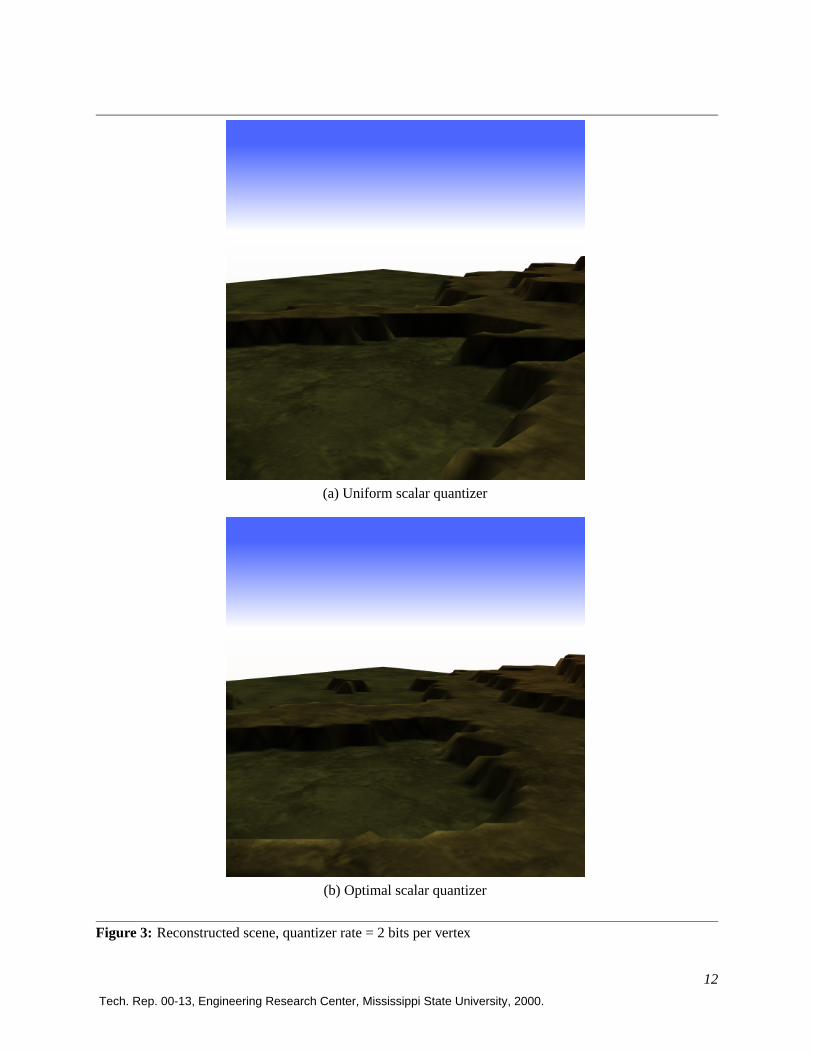
From Fig. 2, we observe that the optimal quantizer offers a modest improvement in PSNR over theuniform quantizer at most of the rates considered. The question at hand then is whether this amount ofgain is significant, given that the ultimate gauge of the quality of the reconstructed terrain dataset is notPSNR measurements between the reconstructed and original height fields, but rather the visual quality ofthe rendered output. In Figs. 3 through 6, we show a scene rendered from the reconstructed terrain for avariety of quantizer rates for both uniform and optimal quantization strategies. This scene has a mixture ofboth flat-land and ridge terrain features. For quantization under 6 bits per vertex, distortion of the terrain isquite visible—ridge and mountain features exhibit sharp variations in slope while small undulations in theterrain are lost. This distortion occurs for both quantization strategies, with the optimal quantizer perhapsproducing slightly better looking results at very low rates (2 and 4 bits per vertex). However, very littledifference is evident between the images for quantizer rates of 6 bits and over. In addition, the images forboth strategies are essentially visually lossless for these higher rates when compared to the original (non-quantized) terrain. Similar results were observed for other regions in the terrain, suggesting that perceptuallynear-lossless terrain rendering is possible at around 6 to 8 bits per vertex, corresponding to a compressionratio of 24:1 to 32:1 in comparison to the size of the original dataset representation (192 bits per vertex).Additionally, we observe that, although the optimal quantizer produces slightly better PSNR, for usefulrates (for which distortion is not visually significant, 6 to 8 bits per vertex and above), no better visualperformance is obtained, despite the extra computation involved in designing the optimal quantizer anddecoding the optimally quantized representation.

Finally, we observe that Deering’s “rule of thumb” of 16 bits per vertex [4] as an upper bound on tolera-ble quantization rate is perhaps rather loose. Our observations indicate that much greater compression, on theorder of 6 to 8 bits per vertex, is visually lossless in situations we have considered. This is particularly truefor common rendering applications involving terrains, such as fly-throughs and browsing. In our application,fly-throughs using 6-bit quantization yielded animations of high quality; sample animations in MPEG formatare available at http://www.erc.msstate.edu/labs/vail/projects/terrain_render.html

6. ConclusionsIn this paper, we presented encoding techniques for representing vertex coordinates of a terrain model.In particular, we examined the suitability of uniform and optimal quantization. Uniform quantization hasthe advantage of being amenable to incorporation in the hardware graphics-rendering pipeline as inverse

10

Tech. Rep. 00-13, Engineering Research Center, Mississippi State University, 2000.

0 1 2 3 4 5 6 7 80

5

10

15

20

25

30

35

40

45

50

Quantizer Rate (bits per vertex)

PS

NR

(dB

)

UniformOptimal

Figure 2: Rate-distortion performance of the proposed approach to quantization.

quantization can be achieved there via a simple matrix operation. Thus, our simple technique bridges thegap between efficient data representation and timely rendering of very large terrain data. In our case, therendering of a very large terrain which could not otherwise be ingested into the memory subsystems of manycommercial graphics hardware was made possible. In addition, our results argue that uniform quantizationprovides the same level of accuracy as the optimal-quantization scheme for terrain datasets. Surprisingly,we found that a 6-bit quantizer suffices for datasets we considered, much fewer bits than the 16 bits ofquantization that Deering [4] observed as being sufficient for viable geometric encoding. Although wefocused on terrain models here, our technique can form the trailing end of any polygonal simplificationtechnique, as quantization plays a fundamental role in the larger paradigm geometric compression. Finally,the work presented here can be viewed as providing a rigorous link between the precision requirements ofmodeling and those of rendering.

In the future, we intend to explore the addition of other compression and coding techniques to theapproach outlined here to allow very succinct storage on hardware disks or expedient transmission throughlow-bandwidth networks. We are particularly interested in the design of encoding techniques that bothpreserve geometrical properties of the terrain and exploit the underlying hardware rendering pipeline. Weintend to seek answers by resorting to appropriate rate-distortion techniques that are in vogue in the image-processing community.

11

Tech. Rep. 00-13, Engineering Research Center, Mississippi State University, 2000.

(a) Uniform scalar quantizer

(b) Optimal scalar quantizer

Figure 3: Reconstructed scene, quantizer rate = 2 bits per vertex

12

Tech. Rep. 00-13, Engineering Research Center, Mississippi State University, 2000.

(a) Uniform scalar quantizer

(b) Optimal scalar quantizer

Figure 4: Reconstructed scene, quantizer rate = 4 bits per vertex

13

Tech. Rep. 00-13, Engineering Research Center, Mississippi State University, 2000.

(a) Uniform scalar quantizer

(b) Optimal scalar quantizer

Figure 5: Reconstructed scene, quantizer rate = 6 bits per vertex

14

Tech. Rep. 00-13, Engineering Research Center, Mississippi State University, 2000.

(a) Uniform scalar quantizer

(b) Optimal scalar quantizer

Figure 6: Reconstructed scene, quantizer rate = 8 bits per vertex

15

Tech. Rep. 00-13, Engineering Research Center, Mississippi State University, 2000.

References

[1] H. Hoppe, “Progressive Meshes,” in SIGGRAPH ’96 Proc., August 1996, pp. 99–108.

[2] M. Reddy, Y. Leclerc, L. Iverson, and N. Bletter, “TerraVision II: Visualizing Massive Terrain Databasesin VRML,” IEEE Computer Graphics and Applications, vol. 19, no. 2, pp. 30–38, March/April 1999.

[3] R. Pajarola, “Large Scale Terrain Visualization Using The Restricted Quadtree Triangulation,” inProceedings of the IEEE Visualization Conference, October 1998, pp. 19–26.

[4] M. Deering, “Geometry Compression,” in SIGGRAPH ’95 Proc., August 1995, pp. 13–20.

[5] G. Taubin and J. Rossignac, “Geometric Compression through Topological Surgery,” ACM Transactionson Graphics, vol. 17, no. 2, pp. 84–115, April 1998.

[6] P. S. Heckbert and M. Garland, “Survey of Polygonal Surface Simplification Algorithms,” CarnegieMellon University Technical Report, Pittsburgh, PA, May 1997, also presented as part of the Mutireso-lution Surface Modeling Course, SIGGRAPH ’97.

[7] D. A. Huffman, “A Method for the Construction of Minimum-Redundancy Codes,” Proceedings of theIRE, vol. 40, no. 9, pp. 1098–1101, September 1952.

[8] I. H. Witten, R. M. Neal, and J. G. Cleary, “Arithmetic Coding for Data Compression,” Communicationsof the ACM, vol. 30, no. 6, pp. 520–540, June 1987.

[9] A. Gersho and R. M. Gray, Vector Quantization and Signal Compression, Kluwer international seriesin engineering and computer science. Kluwer Academic Publishers, Norwell, MA, 1992.

16