206
Decomposing and Regenerating Syntactic Trees Federico Sangati
Decomposing and RegeneratingSyntactic Trees
Federico Sangati


Decomposing and RegeneratingSyntactic Trees
ILLC Dissertation Series DS-2012-01
For further information about ILLC-publications, please contact
Institute for Logic, Language and ComputationUniversiteit van Amsterdam
Science Park 9041098 XH Amsterdam
phone: +31-20-525 6051fax: +31-20-525 5206e-mail: [email protected]
homepage: http://www.illc.uva.nl/

Decomposing and RegeneratingSyntactic Trees
Academisch Proefschrift
ter verkrijging van de graad van doctor aan deUniversiteit van Amsterdam
op gezag van de Rector Magnificusprof. dr. D. C. van den Boom
ten overstaan van een door het college voorpromoties ingestelde commissie, in het openbaar
te verdedigen in de Agnietenkapelop donderdag 12 januari 2012, te 10.00 uur
door
Federico Sangati
geboren te Abano Terme, Italie.

Promotiecommissie:
Promotor:prof. dr. L.W.M. BodCo-promotor:dr. W.H. Zuidema
Overige leden:prof. dr. P.W. Adriaansdr. T. Cohnprof. dr. S. Kahaneprof. dr. R.J.H. Schadr. K. Sima’an
Faculteit der GeesteswetenschappenUniversiteit van Amsterdam
The research reported in this thesis was supported through a Vici-grant “Integrat-ing Cognition” (nr. 277.70.006) to Rens Bod by the Netherlands Organizationfor Scientific Research (NWO).
Copyright © 2012 by Federico Sangati
Printed and bound by Ipskamp Drukkers
ISBN: 978–90–5776–234–5

all’Italia del dopo Berlusconiperche si possa finalmente risvegliare dal lungo sonno
v

Contents
Acknowledgments xi
1 Introduction 11.1 Learning Language Structures . . . . . . . . . . . . . . . . . . . . . . 2
1.1.1 The hidden structure of language . . . . . . . . . . . . . . . . 21.1.2 Different perspectives on language . . . . . . . . . . . . . . . 3
1.2 Syntactic structures of language . . . . . . . . . . . . . . . . . . . . . 41.2.1 Syntactic representation and generative processes . . . . . . 41.2.2 Different representations . . . . . . . . . . . . . . . . . . . . . 51.2.3 Phrase-Structure . . . . . . . . . . . . . . . . . . . . . . . . . . 51.2.4 Dependency-Structure . . . . . . . . . . . . . . . . . . . . . . 61.2.5 Relations between PS and DS . . . . . . . . . . . . . . . . . . 7
1.3 Generative models of syntactic structures . . . . . . . . . . . . . . . 71.3.1 Context-Free Grammars . . . . . . . . . . . . . . . . . . . . . 81.3.2 Generalized models . . . . . . . . . . . . . . . . . . . . . . . . 81.3.3 Probabilistic generative models . . . . . . . . . . . . . . . . . 10
1.4 Computational models of syntax . . . . . . . . . . . . . . . . . . . . 111.5 Thesis overview . . . . . . . . . . . . . . . . . . . . . . . . . . . . . . . 14
2 Generalized Tree-Generating Grammars 172.1 Introduction . . . . . . . . . . . . . . . . . . . . . . . . . . . . . . . . . 18
2.1.1 Symbolic and Probabilistic models . . . . . . . . . . . . . . . 182.1.2 Tree structures . . . . . . . . . . . . . . . . . . . . . . . . . . . 20
2.2 Symbolic Generative Models for Trees . . . . . . . . . . . . . . . . . 222.2.1 The event space . . . . . . . . . . . . . . . . . . . . . . . . . . 222.2.2 The conditioning context . . . . . . . . . . . . . . . . . . . . . 232.2.3 Context-Free Grammar . . . . . . . . . . . . . . . . . . . . . . 242.2.4 The generative process . . . . . . . . . . . . . . . . . . . . . . 252.2.5 Extracting a symbolic grammar from a treebank . . . . . . 30
vii

2.2.6 Examples of generative tree grammars . . . . . . . . . . . . . 302.3 Probabilistic Generative Models for Trees . . . . . . . . . . . . . . . 38
2.3.1 Resolving the syntactic ambiguity . . . . . . . . . . . . . . . 382.3.2 The probability of a tree . . . . . . . . . . . . . . . . . . . . . 392.3.3 Estimating Probability Distributions . . . . . . . . . . . . . . 39
2.4 Parsing through Reranking . . . . . . . . . . . . . . . . . . . . . . . . 432.5 Discriminative and Generative models . . . . . . . . . . . . . . . . . 442.6 Conclusions . . . . . . . . . . . . . . . . . . . . . . . . . . . . . . . . . 47
3 Recycling Phrase-Structure Constructions 493.1 Introduction to Phrase-Structure . . . . . . . . . . . . . . . . . . . . 503.2 Review of existing PS models . . . . . . . . . . . . . . . . . . . . . . 51
3.2.1 Head-driven models . . . . . . . . . . . . . . . . . . . . . . . . 513.2.2 State-Splitting Models . . . . . . . . . . . . . . . . . . . . . . 53
3.3 Data-Oriented Parsing . . . . . . . . . . . . . . . . . . . . . . . . . . . 543.3.1 Introduction . . . . . . . . . . . . . . . . . . . . . . . . . . . . 55
3.4 The symbolic backbone . . . . . . . . . . . . . . . . . . . . . . . . . . 563.4.1 Explicit vs. Implicit Grammars . . . . . . . . . . . . . . . . . 56
3.5 Finding Recurring Fragments . . . . . . . . . . . . . . . . . . . . . . 583.5.1 The search algorithm . . . . . . . . . . . . . . . . . . . . . . . 593.5.2 A case study on the Penn WSJ . . . . . . . . . . . . . . . . . 60
3.6 The probability model . . . . . . . . . . . . . . . . . . . . . . . . . . . 663.6.1 Parsing . . . . . . . . . . . . . . . . . . . . . . . . . . . . . . . 673.6.2 Inducing probability distributions . . . . . . . . . . . . . . . 693.6.3 Maximizing Objectives . . . . . . . . . . . . . . . . . . . . . . 70
3.7 Implementation . . . . . . . . . . . . . . . . . . . . . . . . . . . . . . . 733.8 Annotated Resources . . . . . . . . . . . . . . . . . . . . . . . . . . . 753.9 Evaluation Metrics . . . . . . . . . . . . . . . . . . . . . . . . . . . . . 763.10 Results . . . . . . . . . . . . . . . . . . . . . . . . . . . . . . . . . . . . 763.11 Conclusions . . . . . . . . . . . . . . . . . . . . . . . . . . . . . . . . . 83
3.11.1 Future Directions . . . . . . . . . . . . . . . . . . . . . . . . . 833.11.2 Next steps . . . . . . . . . . . . . . . . . . . . . . . . . . . . . 84
4 Learning Dependency-Structures 854.1 Introduction . . . . . . . . . . . . . . . . . . . . . . . . . . . . . . . . . 864.2 Dependency-Structure . . . . . . . . . . . . . . . . . . . . . . . . . . . 874.3 Comparing PS with DS . . . . . . . . . . . . . . . . . . . . . . . . . . 88
4.3.1 Structural relations between PS and DS . . . . . . . . . . . . 884.3.2 Relations between PS and DS grammars . . . . . . . . . . . 90
4.4 Other related syntactic theories . . . . . . . . . . . . . . . . . . . . . 924.5 Models for parsing DS . . . . . . . . . . . . . . . . . . . . . . . . . . . 95
4.5.1 Probabilistic Generative models . . . . . . . . . . . . . . . . 954.5.2 Discriminative models . . . . . . . . . . . . . . . . . . . . . . 99
viii
4.6 Reranking generative models . . . . . . . . . . . . . . . . . . . . . . . 1004.6.1 Experiment Setup . . . . . . . . . . . . . . . . . . . . . . . . . 1024.6.2 Comparing the Eisner models . . . . . . . . . . . . . . . . . . 1024.6.3 A new generative model . . . . . . . . . . . . . . . . . . . . . 1034.6.4 Results . . . . . . . . . . . . . . . . . . . . . . . . . . . . . . . 105
4.7 Conclusions . . . . . . . . . . . . . . . . . . . . . . . . . . . . . . . . . 1074.8 Future Directions . . . . . . . . . . . . . . . . . . . . . . . . . . . . . . 108
5 Tesniere Dependency-Structure 1095.1 Introduction . . . . . . . . . . . . . . . . . . . . . . . . . . . . . . . . . 1105.2 Dependency-Structures a la Tesniere . . . . . . . . . . . . . . . . . . 111
5.2.1 The dependency relation . . . . . . . . . . . . . . . . . . . . . 1115.2.2 Words, blocks and categories . . . . . . . . . . . . . . . . . . 1115.2.3 Junction . . . . . . . . . . . . . . . . . . . . . . . . . . . . . . . 1125.2.4 Transference . . . . . . . . . . . . . . . . . . . . . . . . . . . . 113
5.3 Comparing TDS with DS . . . . . . . . . . . . . . . . . . . . . . . . . 1145.3.1 Choosing the correct heads . . . . . . . . . . . . . . . . . . . 1165.3.2 Categories and Blocks . . . . . . . . . . . . . . . . . . . . . . 1165.3.3 Coordination . . . . . . . . . . . . . . . . . . . . . . . . . . . . 117
5.4 Converting the Penn WSJ in TDS notation . . . . . . . . . . . . . . 1185.4.1 Elements of a TDS . . . . . . . . . . . . . . . . . . . . . . . . 1185.4.2 The conversion procedure . . . . . . . . . . . . . . . . . . . . 119
5.5 A probabilistic Model for TDS . . . . . . . . . . . . . . . . . . . . . . 1215.5.1 Model description . . . . . . . . . . . . . . . . . . . . . . . . . 1215.5.2 Experimental Setup . . . . . . . . . . . . . . . . . . . . . . . . 1235.5.3 Evaluation Metrics for TDS . . . . . . . . . . . . . . . . . . . 1245.5.4 Results . . . . . . . . . . . . . . . . . . . . . . . . . . . . . . . 125
5.6 Other representations of the WSJ Treebank . . . . . . . . . . . . . . 1265.6.1 Prague English dependency treebank . . . . . . . . . . . . . 1285.6.2 Stanford Typed Dependency Representation . . . . . . . . . 1285.6.3 Bubble Trees . . . . . . . . . . . . . . . . . . . . . . . . . . . . 1315.6.4 The CCG-bank . . . . . . . . . . . . . . . . . . . . . . . . . . 131
5.7 Assessment of the converted treebank . . . . . . . . . . . . . . . . . 1335.8 Conclusion . . . . . . . . . . . . . . . . . . . . . . . . . . . . . . . . . . 1345.9 Future directions . . . . . . . . . . . . . . . . . . . . . . . . . . . . . . 134
6 Conclusions 137
A Phrase-Structure Models 141A.1 Models parameters . . . . . . . . . . . . . . . . . . . . . . . . . . . . . 141A.2 Evaluation procedure . . . . . . . . . . . . . . . . . . . . . . . . . . . 142A.3 Comparing Double-DOP and Berkeley parser . . . . . . . . . . . . . 144
ix

B Dependency-Structure Models 145B.1 DS to PS . . . . . . . . . . . . . . . . . . . . . . . . . . . . . . . . . . . 145B.2 Smoothing details . . . . . . . . . . . . . . . . . . . . . . . . . . . . . 147
C TDS model 149C.1 Head annotation . . . . . . . . . . . . . . . . . . . . . . . . . . . . . . 149C.2 Coordination . . . . . . . . . . . . . . . . . . . . . . . . . . . . . . . . 151C.3 Smoothing in the TDS model . . . . . . . . . . . . . . . . . . . . . . 155C.4 Examples of TDS trees . . . . . . . . . . . . . . . . . . . . . . . . . . 155
Bibliography 160
Index 183
Samenvatting 185
Abstract 187
x

Acknowledgments
I am very grateful to Rens Bod and Jelle Zuidema for their supervision. Theircomplementary roles were fundamental for the development of my research. Sincethe beginning of my PhD, Rens has shown lot of trust and confidence in my ca-pabilities and has let me total freedom in exploring various research paths, yetproviding me solid guidance in moments of need. This has allowed me to learnhow to work independently and understand my real research interests. Jelle’spresence was also indispensable throughout the whole project: he has great pa-tience as a listener, and a remarkable ability to quickly understand a problemand formulate brilliant solutions. But above all his intellectual honesty, and hisability to relativize things within and outside academia made him one of the mostrelevant guiding figures in all these years.
I am thankful to a number of people who have accompanied me during thelast four years. In particular the PhD members of the LaCo group: GideonBorensztajn with whom I’ve shared the whole PhD adventure, including manymoments of intense discussions, big struggles, exciting ping-pong challenges, andother fun activities; Markos Mylonakis great hiking companion as well as irre-placeable machine learning advisor; Gideon Maillette de Buy Wenniger for thenice discussions and his big courage in taking over and extending my GUI code;and Barend Beekhuizen for his great passion and for his invaluable help in anno-tating hundreds of sentences.
I am in debt with Yoav Seginer one of the most significant teachers who haveinspired me during the beginning of my PhD, and accepted to go through thepre-final draft of my thesis (long after having left academia) providing extremelyvaluable feedbacks. Many thanks to Chiara Mazza for the fruitful collaborationstarted during the summer 2009 which has lead to the joint work on TesniereDependency Structures; and to Andreas van Cranenburgh, for the intense inter-action towards the end of my project, and for the effort of proof-reading the thesisand translating the abstract into Dutch.
Special thanks to Pieter Adriaans, Remko Scha, Khalil Sima’an, and Henk
xi

Zeevat from whom I’ve learned a lot since I came to Amsterdam for the MSc.In the last few years they have continued supporting my work and frequentlyprovided me with valuable feedbacks in dedicated meetings and dry runs. Manythanks also to the external members of the PhD committee Trevor Cohn andSylvain Kahane for their numerous comments and suggestions on the thesis.
I am grateful to other colleagues with whom I had the pleasure to build fruitfuldiscussions in Amsterdam and abroad: Tejaswini Deoskar, Yoav Goldberg, GeroldSchneider, Djame Seddah, and Reut Tsarfaty.
Next, I would like to express profound gratitude to my paranymphs InesCrespo and Umberto Grandi for their assistance in completing all the proceduressurrounding the end of my PhD, but above all for having represented solid figuresof support in times of struggle, and great companions in several activities we havegone through the last few years.
A collective thank you to all the other colleagues at the ILLC, with whomI have shared interesting conversations, coffees, and many laughs: StephaneAiriau, Sophie Arnoult, Cedric Degremont, Ulle Endriss, Marıa Esteban Garcia,Vanessa Ferdinand, Stefan Frank, Pietro Galliani, Nina Gierasimczuk, DavideGrossi, Aline Honingh, Tikitu de Jager, Yurii Khomskii, Lena Kurzen, DanielePorello, Michael Repplinger, Raul Leal Rodriguez, Raquel Fernandez Rovira, San-chit Saraf, Mehrnoosh Sadrzadeh, Maria Spychalska, Jakub Szymanik, Joel andSara Uckelman, Fernando Raymundo Velazquez-Quesada, and Jacob Vosmaer.
I would like to also thank the ILLC administrators for their indispensable sup-port: Karin Gigengack, Tanja Kassenaar, Ingrid van Loon, Peter van Ormondt,and Marco Vervoort.
A big thank you to the Nuts Ultimate Frisbee teammates, for having sharedlot of fun practices and games throughout the last two years.
Finally I intend to express my affection and gratitude to all those peoplewho have continuously supported me during all these years and contributed toenrich my life: my parents, Andrea and Marco Sangati, Irene Bertazzo, PaipinCheng, Winnie & Renee, Chiara Brachini, Daniil Umanski, Lisa Kollwelter, Mar-got Colinet, Pablo Seban, Giulia Soravia, Martina Deana, Ermanno Miotto, SaraSambin, Tino Ginestri, and the Pablo Neruda group.
It is extremely difficult to give full acknowledgments to all the people who havedirectly or indirectly contributed to the completion of my PhD, so I apologize ifsomeone has been accidentally omitted or hasn’t been given the appropriate rel-evance.
Edinburgh Federico SangatiNovember, 2011.
xii

The word of man is the most durable of all material.
Arthur Schopenhauer
Chapter 1Introduction
1

2 Chapter 1. Introduction
1.1 Learning Language StructuresDuring the last decades, research in Natural Language Processing (NLP) seemsto have increasingly lost contact with linguistic theory, as Mark Steedman hasstated:
“[...] while from the 1950s to the 1980s, the information theoreticians andstatistical modelers among us used to make common cause with the linguists, wehave subsequently drifted apart.” (Steedman, 2008, p. 139)
The current thesis can be seen as a reaction to this observation: it aims atbuilding computational models of syntax based on a number of basic linguistictheories showing that, contrary to common wisdom, their notions and conceptscan be highly beneficial to NLP. This work is not meant to provide any finalassessment for the validity of the theories under consideration, but should ratherbe seen as an attempt to formalize and understand them better. A second goalof this thesis is to contribute to the development of computer systems which aimat solving linguistic tasks, for which syntax plays an important role.
In this introductory chapter we will provide some background to the ongoingquest of discovering the hidden structures of language, and the role that compu-tational models can play in accomplishing this goal.
1.1.1 The hidden structure of languageLanguage is one of the most acknowledged traits of human beings: it pervades ineveryday life, and it has existed across all cultures for thousands of generations.Nevertheless, language remains one of the most controversial subjects of inquiry.Language is in fact a vague concept, hard to map to a precise entity which canbe scientifically investigated. It is dynamic, as it changes in time and acrosslinguistic communities, and there is no way to isolate it as a whole: even if wecould sample all human utterances for the next 100 years we would only cover avery small fraction of all possible language productions.
Moreover, language exists in different modalities, i.e., oral, gestural, and writ-ten. Within each of these modalities, an external observer has access only to thesurface manifestation of language, i.e., sound, gestures, and text. But surfaceinformation cannot fully account for what we describe as language: as in othercognitive abilities, external manifestations are only the tip of the iceberg. Thestructures1 underlying language productions remain well hidden,2 and although
1A language structure, in general, describes how the parts of a language production arerelated and built into a whole.
2Although there is also some dispute about the actual existence of underlying structures inlanguage, we decided not to enter into this debate. It should suffice to say that language asother complex dynamical systems is constantly shaped by many forces, and the regularity it
1.1. Learning Language Structures 3
regular patterns in the surface layer may provide useful clues for building hy-potheses on the hidden ones, there is no precise way to verify if the linguisticanalysis matches the representation used by the speaker. This observation wasalready made by Ferdinand de Saussure, who wrote about word categories (nouns,adjectives, etc.):
“All these things exist in language, but as abstract entities; their study isdifficult because we never know exactly whether or not the awareness of speakersgoes as far as the analyses of the grammarian.” (de Saussure, 1915, p. 190)
1.1.2 Different perspectives on languageLanguage can be studied using a wide variety of methodologies. In theoreticallinguistics one of the most dominant modus operandi is the introspective approach(Tesniere 1959, p. 37; Chomsky 1984, p. 44). Under this perspective, any personwho attempts to investigate language is not only seen as an external observer, butalso as an active language user. He/she is therefore able to construct hypotheseson language structures based on internal intuitions, and assess how well theygeneralize, relying on internal judgements.
In contrast to this approach, the investigation of language has included muchexperimental research, whose objective is to validate hypotheses about the struc-ture of language, based on experimental data obtained from language users per-formance in specific tasks, such as sentence processing (Hale, 2006; Levy, 2007;Frank and Bod, 2011), or acquisition of phonology and morphology (Boersmaand Hayes, 2001; Goldwater et al., 2007), as well as from brain activations onlinguistic stimuli (Bachrach, 2008).
But ultimately, both introspective and experimental approaches could provideonly a partial description of the investigated phenomenon. Language, in fact, isa means of communication, and as such it is not confined to any specific organor individual. It is a dynamic system whose behavior can be explained onlywhen considering the system as a whole, including the speaking community, thecommunicative interactions established between its members, and the externalenvironment they share. Fortunately, there are other approaches to languagewhich try to give accounts for its dynamic aspects. These include fields such aslanguage evolution (Lieberman, 1975; Zuidema, 2005), sociolinguistics (Labov,1972; Wardhaugh, 2006), historical linguistics, and language change (Lass, 1997).
The abundance of perspectives on the study of language reflects the enormouscomplexity of this phenomenon. As all of these theories are small pieces of thesame puzzle, it is important to develop methodologies which attempt to integratethem in order to build a basis for a unified theory. Unfortunately, in the current
exhibits is a strong evidence for the existence of underlying structures.

4 Chapter 1. Introduction
state of affairs, there is a tendency for each perspective to develop independentlyfrom the others.
The current work is not entirely excluded from this critique, as the modelswhich will be presented are all based on static perspectives on language andthey only focus on syntax. However, one of the primary goals of this work is toprovide a bridge between computational models and traditional syntactic theoriesof language, two approaches which are increasingly diverging from each other.We are strongly in favor of a more shared agenda between syntacticians andcomputational linguists and in §1.4 we illustrate a possible way to achieve this.
1.2 Syntactic structures of languageIn this thesis we will focus on a number of syntactic models of language. Syntaxis the study of the rules governing the construction of phrases and sentencesin natural languages. Most existing syntactic theories analyze language at anintermediate level: they assume words as the elementary units of production, andsentences as the largest elements under investigation. This is a strong simplifyingassumption, as there are processes both below word level and above sentence level,which cannot be considered entirely independent from syntax. This separationis justified as the first step for isolating the phenomenon under study, i.e., therules for describing how words are put together to form sentences. Ultimately,any syntactic theory should still define bridges to other levels of analysis, such asphonetics, phonology and morphology (below word level), as well as pragmatics,prosody and discourse-processing (above word and sentence level).
Semantics is another linguistic field which studies the meaning of languageproductions. Similarly to syntax, semantics typically analyzes language at theintermediate level between word and sentence boundaries. As there is a greatamount of overlapping concepts between the two fields, their separation is some-how artificial, and varies upon the definition of the linguistic theories within thetwo domains.
1.2.1 Syntactic representation and generative processesAlthough the tradition of investigating language syntax can be dated back toPanini’s work (circa 5th century BC), the discussion about which theory we shoulduse is still open. Any syntactic theory presupposes a certain type of structurebeyond the directly observable utterances, and attempts to explain how to mapthe surface form, i.e., the sequence of words in the sentence, into the hiddenrepresentation. It is therefore important to distinguish between the syntacticrepresentation of a theory, i.e., the type of syntactic structures it presupposes, andits generative model, i.e., the description of the way to construct them. Certaintheories may remain incomplete in this respect, typically focusing only on the
1.2. Syntactic structures of language 5
representation (e.g., Tesniere, 1959). A complete syntactic theory should aimat describing both aspects as formally as possible, in order to be unambiguous.We will start by introducing the representational part of syntax, and further on(in §1.3) proceed to describe its generative account.
1.2.2 Different representationsIn this thesis we will adopt two main classes of syntactic theories, characterized bytwo different representations: phrase-structure (PS, also known as constituencystructures), and dependency-structure (DS). Historically, these two theories haveemerged around the same time during the 1950s: PS in the U.S. with NoamChomsky (1957), and DS in continental Europe with the somewhat lesser knownLucien Tesniere (1959). Neither Chomsky nor Tesniere formulated their respec-tive theories from scratch, but owed a lot to previous work: Chomsky inheritedthe notion of (Immediate) Constituency from Wundt (1900), Bloomfield (1933),Wells (1947), and Harris (1951), while Tesniere borrowed several concepts andmethods from de Saussure (1915).
In parallel and after the foundational work of Chomsky and Tesniere, a vastnumber of other syntactic theories have been developed, considered more deepthan either PS or DS, such as Categorial Grammars (Ajdukiewicz, 1935; Bar-Hillel, 1953), LFG (Bresnan, 2000; Dalrymple, 2001), HPSG (Pollard et al., 1994),TAG (Joshi, 1985), Word Grammars (Sugayama and Hudson, 2005), MeaningText Theory (Mel’cuk, 1988) and many others (we will review some of themin §4.4 and §5.6). Our choice to focus on DS and PS is justified by the needto compromise between the possibility of defining data-driven parsing algorithmson the one hand, and using linguistically adequate representations on the other.Although there is continuous effort to parse with deep linguistic analyses (e.g.,Riezler et al., 2002; Bod and Kaplan, 2003), it is not easy to translate theseformalisms into data-driven parsing models, both for their complexity, and forthe shortage of corpora directly annotated with these representations.
However, in our approach, rather than committing to a single syntactic analy-sis, we are interested in taking several approaches in parallel. We are in fact quiteagnostic about what is the “correct representation”, and we therefore advocatefor the integration of different perspectives as a way to obtain a more completesyntactic description. In the remaining part of this section we will introduce andcompare the PS and DS representations.
1.2.3 Phrase-StructureIn a phrase-structure (PS) representation, the words of a sentence are groupedin hierarchical constituents (or phrases): a sequence of words, functioning as asingle unit, is grouped into a basic constituent; adjacent constituents are groupedinto higher phrases forming a hierarchical structure, whose highest level spans
6 Chapter 1. Introduction
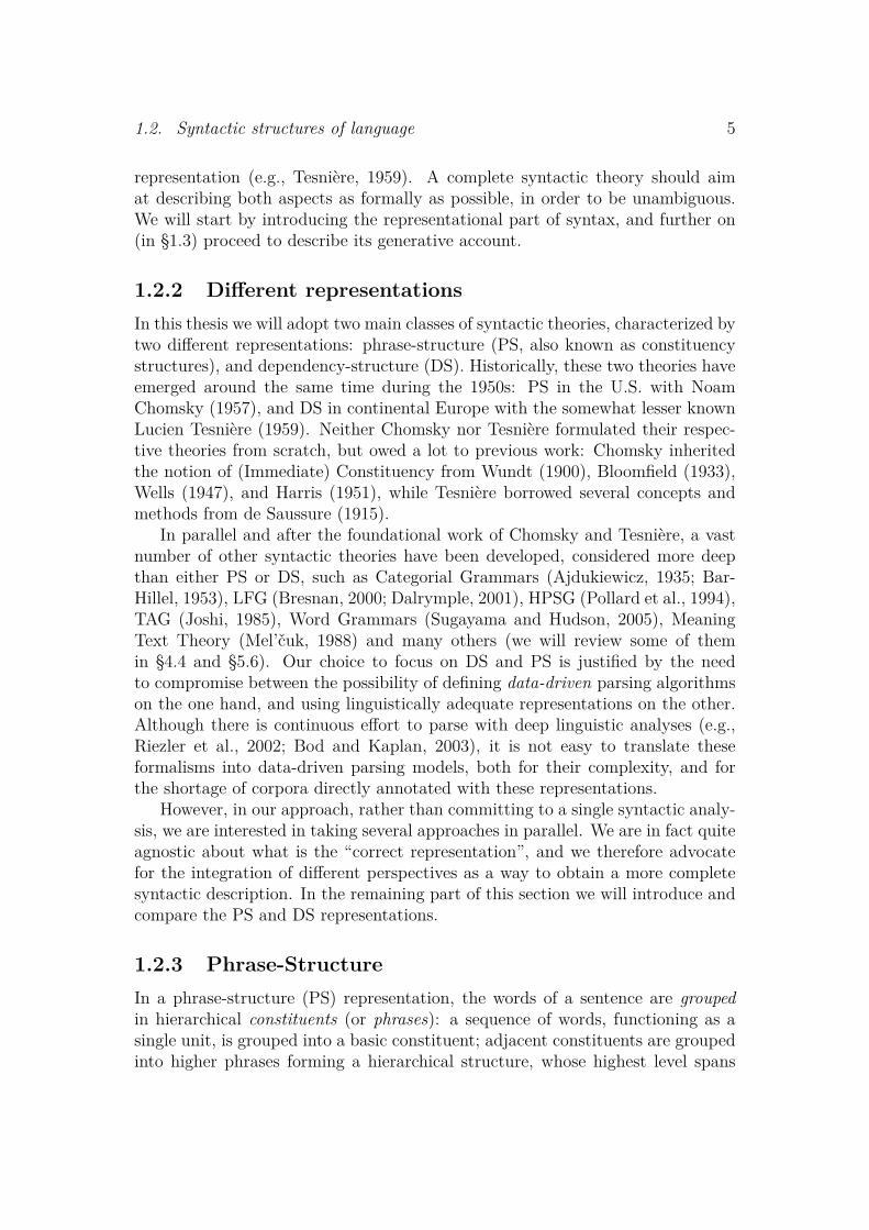
all the words in the sentence. For instance, the sentence “My old friend sangthis nice song” can be mapped into the PS reported in figure 1.1. A more typical(yet isomorphic) tree representation for this structure is shown in figure 1.2, whereevery non-terminal node uniquely maps to a box in the representation of figure 1.1.The non-terminal nodes in a PS tree are usually assigned categorial labels, suchas NP (noun phrase), and VP (verb phrase). A version of the same tree withsuch labels is illustrated in figure 1.4 (left), and will become more relevant whenwe will introduce a generative account for PS.
My old friend sang this nice song
Figure 1.1: Structure of the sentence “My old friend sang this nice song”, accord-ing to a phrase-structure (PS) representation.
My old friend sang
this nice song
Figure 1.2: Example of the PS in figure 1.1 in an equivalent tree representation:each box in the former representation corresponds to a non-terminal node of thistree.
1.2.4 Dependency-StructureIn a dependency-structure (DS) representation, words of a sentence are related toone another (instead of being grouped together as in PS). For every two wordsA and B in the sentence, there can be a dependency relation. If this relationexists, we say that one of the two words, say B, is a dependent or modifier of A,while A is the governor or head of B. Roughly speaking, B is a dependent of Aif its presence is only justified by the presence of A, and only if B modifies themeaning of A. All words in a sentence should be connected directly or indirectlyby dependency relations forming a dependency tree, having a single word as theroot of the structure (usually the main verb of the sentence), which governsdirectly or indirectly all other words.
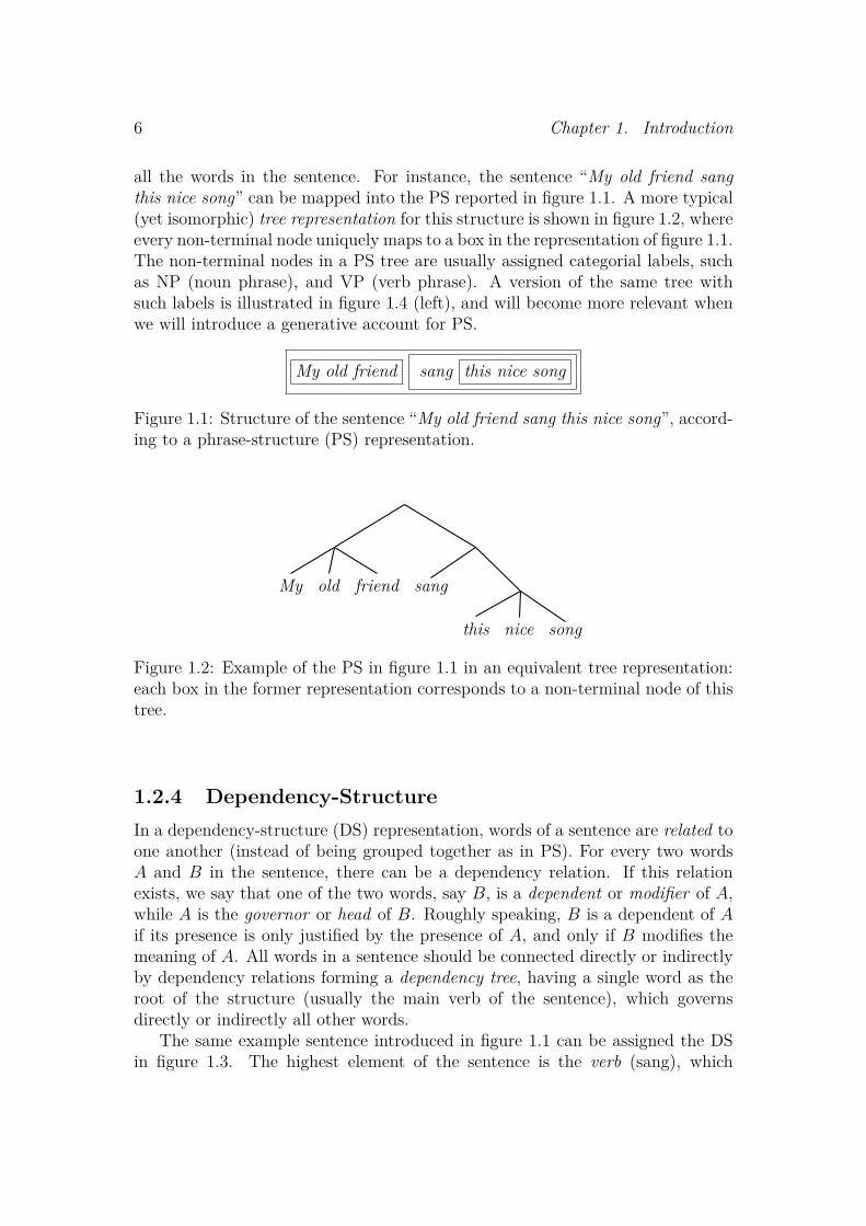
The same example sentence introduced in figure 1.1 can be assigned the DSin figure 1.3. The highest element of the sentence is the verb (sang), which

1.3. Generative models of syntactic structures 7
has two direct dependents: the actor of the singing (friend) and what has beensung (song). Moreover, the noun ‘friend’ is modified by two dependents (my, old),which specify further qualities of the noun. Analogously ‘song’ is modified by twoother dependents (this, nice). It is important to remark that in this simplifiedDS representation the order of the words is not preserved, but in the DS trees wewill employ, word order will be specified (see §2.1.2 and chapter 4).
sang
friend
my old
song
this nice
Figure 1.3: Dependency-Structure of the sentence “My old friend sang this nicesong”, according to Tesniere notation (Tesniere, 1959, p. 14).
1.2.5 Relations between PS and DSPS and DS are based on different types of structure. PS assumes the notion ofhierarchical phrases as abstract entities at intermediate levels of the tree structure.No such grouping is postulated in DS, as words are placed in all the nodes of thetree, and relations between words are the only assumed abstract entities. But weargue that there is no reason to claim the exclusive validity of PS or DS, sinceeach notation focuses on a specific aspect of syntax, viz. grouping vs. relations.
There are, however, more similarities between PS and DS than apparent froma first look. In fact, as will become more clear in later chapters, the two sys-tems are not incompatible with one another, as it is possible to define specifictransformations for converting one representation into the other (see §4.3.1), andeven define syntactic structures which include both notions of constituents anddependencies (see chapter 5).
1.3 Generative models of syntactic structuresAfter defining the structural representation of sentences, a syntactic theory shouldprovide a rigorous account for how sentence structures are constructed. Theseminal work of Chomsky (1956, 1957) has represented a major turning point inmodern linguistics in this sense, as it was the first successful attempt of deriving aformal theory of syntax, characterized by the introduction of generative models,3which can be described as algebraic machineries for deriving sentence structures.
3The work of Harris (1951) includes the first description of generative grammars for syntax,but Chomsky’s formulation is more complete and formal.

8 Chapter 1. Introduction
1.3.1 Context-Free GrammarsChomsky (1957, ch.4) assumes labeled phrase-structures as the underlying repre-sentation of language syntax, such as the one illustrated in the tree of figure 1.4(left), and describes a system for generating them, also known as Context-FreeGrammar (CFG). A CFG is defined4 as a finite set of rewriting rules, such as theones illustrated in figure 1.4 (right), each characterized by a single non-terminalon the left-hand side of the arrow, which rewrites to any number of non-terminalsand words on the right-hand side of the arrow. Each CFG has a unique startingnon-terminal symbol (typically S) which constitutes the root category of all PStrees the grammar can generate.
A generative model based on a CFG gives an account for how to generateall sentence structures which are compatible with the grammar. The generativeprocess starts with the starting symbol S in the grammar, and chooses a rulerS with S as the left-hand side. This rule will constitute the starting branchingat the root (top) of the tree. Afterwards, for any non-terminal symbol X atthe frontier of the partially constructed tree, the model chooses a rule rX forextending it. This last step is iterated until all the nodes at the bottom of thetree are words (also called terminals, as they cannot rewrite to anything else).
S
NP
My old friend
V P
sang NP
this nice song
S Ð→ NP V PNP Ð→ My old friendV P Ð→ sang NPNP Ð→ this nice song
Figure 1.4: Left: the labeled version of the PS tree in figure 1.2. Right: theContext-Free Grammar for generating the PS tree.
1.3.2 Generalized modelsSo far, we have described generative models only as unidirectional processes:given a grammar, the model can produce all structures compatible with it. Butthe process can be easily reversed: given a set of sentence structures (i.e., atreebank), it is possible to extract a grammar which can generate all observedtrees, and, if general enough, other unobserved ones.
4For a more formal definition of CFGs see §2.2.2.

1.3. Generative models of syntactic structures 9
In the central chapters of this thesis (3, 4, 5), we will take this reverse perspec-tive and make use of hand-annotated treebanks for extracting several generativegrammars.
Models for PS Besides Context-Free Grammars, there is an infinity of othergenerative models for PS that we could take into account. In particular, thereare several limitations implicit in a CFG we would like to solve. A CFG is infact subject to an under-generation problem: the nodes in the right-hand side ofa rule are inseparable from each other, as they are all attached to the derivedtree at the same time, once the rule is applied; a grammar can therefore notgeneralize over its rules. But the CFG rules needed to describe natural sentencescan get arbitrarily long,5 and it is impossible to define them all as the number ofpossible combinations is infinite. At the same time, the derivation process makesa strong independence assumption when combining the rules, as every choice isonly determined by a single node, i.e., the left-hand side of the rule.6 This leads toan over-generation problem: a CFG usually produces, for a given sentence, manysyntactic structures which are not acceptable according to human judgement.
In chapter 2 we will explore a range of different generative models which try tosolve such limitations: for instance we will consider models which generate a PStree one node at a time (instead of attaching all symbols in the right-hand side ofa CFG rule at once) and conditioning every decision on more than a single nodepresent in the partially derived tree, as initially proposed by Magerman (1995),Collins (1997), and Charniak (1997). For each different model, we will need todefine specific elementary units (fragments), and specific operations to combinethem into trees. According to the reversed perspective, for each combinatoryoperation there must be a corresponding deconstruction operation. Given a tree-bank we can therefore decompose all the trees into a set of fragments in order toderive our grammar.
In particular, in chapter 3 we will focus on one specific generative grammarbased on the Data-Oriented Parsing framework (Bod et al., 2003), in which theelementary units are subtrees of unrestricted size extracted from a treebank.
Models for DS More generally, we can also come up with generative modelsfor dependency-structures introduced in §1.2.4. The work of Tesniere (1959), isneither formal nor generative, since it does not provide any algebraic machineryfor describing how to combine words into a sentence structure. This does notmean that it is not possible to derive a formal-generative model based on thistheory. Like PS, in fact, DS can be described as well-formed trees, and this
5There is in principle no upper-bound on the number of nodes in the right-hand side. Forinstance a coordination structure can have an unlimited number of elements which are coordi-nated.
6The severity of this independence assumption can be reduced by including contextual in-formation into the non-terminal labels of the grammar, as discussed in §3.2.2.

10 Chapter 1. Introduction
can allow us to define specific generative models for this representation. In thelast two decades, as the DS representation has become more widely studied incomputational linguistics, several generative models have been proposed (e.g.,Eisner, 1996a,b). In chapter 4 we will review some of these and describe a novelmodel for parsing DS.
However, in order to build a supervised model for dependency-structure, weneed to have access to a collection of consistently annotated DS trees. As thereis no significant manually annotated treebank for the DS representation, we willmake use of standard methodology for automatically converting PS treebanksinto DS notation (see §4.3.1).
However, the resulting DS representation misses several of the fundamentalfeatures which were proposed in the original work of Tesniere (1959), for instance,it does not have a proper way to represent coordination constructions (e.g., “Johnand Mary”). The main contribution of chapter 5 is to propose a more elaboratedversion of dependency-structure which we believe to be more complete with re-spect to Tesniere’s work, and therefore named Tesniere Dependency-Structure(TDS). In particular we will define a conversion procedure for transforming a PStree into a TDS, and propose a generative model for this representation.
1.3.3 Probabilistic generative modelsSo far we have described generative processes which are purely symbolic. A sym-bolic grammar assigns equal degree of grammaticality7 to a set of sentences, i.e.,the ones it can generate. This is in line with Chomsky’s competence paradigm(Chomsky, 1965), according to which native speakers have the internal ability todecide whether a sentence is grammatical or not. This binary perspective hasraised much debate in the last few decades, leading to a performance approachwhich targets the external nature of language communication (Levelt, 1974; Scha,1990; Abney, 1996): language users produce all sort of utterances including thosewhich are not judged entirely sound, but nonetheless constitute real language pro-ductions. According to this perspective the grammaticality of a sentence shouldrange on a continuum rather than discretely.8
There are several possible ways to provide a generative model with a notion ofgrammatical continuity over the generated sentences (and sentence structures).The most commonly adopted strategy, which is followed in this thesis, is to aug-ment the model with a probabilistic component: at each step of the derivationprocess, all available alternative decisions admitted by the grammar are placed
7The notion of grammaticality of a sentence is here tightly related to the notion of accept-ability.
8This graded notion of grammaticality should account for all the factors which make certainsentences more plausible than others. It is in fact common that between two equally soundsentences differing in length, the shorter one is regarded as more acceptable (grammatical)than the other.

1.4. Computational models of syntax 11
in a probabilistic distribution. This gives the means to favor certain choices overothers (if the distribution is not uniform). Constructing and validating a prob-abilistic generative model is nevertheless a difficult task which requires a carefulanalysis for the delicate decisions belonging to both symbolic and statistical do-mains as Klavans and Resnik have stated:
“[...] combining symbolic and statistical approaches to language is a kind ofbalancing act in which the symbolic and the statistical are properly thought ofas parts, both essential, of a unified whole.” (Klavans and Resnik, 1996, p. x)
One of the major benefits of adopting probabilistic models on top of sym-bolic ones is that they allow for solving grammatical ambiguities. In fact, thegrammars which will be extracted from large treebanks easily become extremelyproductive: they generate many novel trees, and many different structures yield-ing the same sentence (see §2.1.1). A probabilistic model implicitly defines aprobability distribution over sentence structures it can generate (obtained fromthe probability of each single decision in the derivation process), and hence itcan place the various alternative structures for a certain sentence in a continuousscale of grammaticality. This can enable us to select the most plausible structureaccording to the model as the most grammatical one.
The process of disambiguating between possible valid structures of the samesentence is essential for two main reasons. First of all we want to be able toevaluate the syntactic theory under investigation, and we can do this only if wehave a single correct analysis (or a restricted set of analyses) for a given sentence.Second, syntactic disambiguation is considered one of the most important tasksfor developing natural language processing applications.
1.4 Computational models of syntaxAs this thesis aims at building computational models of syntax, it is worth reflect-ing what we mean by them and what is their relevance in the study of languagestructures.
Given any formal theory about a real-world phenomenon, we can build acomputational model (CM) for implementing and testing it. The theory needsto be formally defined in order to be integrated into the CM, viz. it needs todescribe precisely how the CM should map any set of partial information to someinformative counterpart. For each experiment, we provide the CM with partialinformation of the observed system, and ask the CM to return novel informationabout the system. Finally, we can quantify in how far the predicted outcomediffers from the observation.
During the last few decades computer models have been adopted in all sci-entific fields: from physics, to astronomy, chemistry and biology, computational

12 Chapter 1. Introduction
approaches are currently used to validate a full range of scientific theories. Oneof the historical examples of computational models in chemistry is DENDRAL(Lindsay et al., 1980), a computer system which aims at determining the molec-ular structure of an organic chemical sample, given its spectroscopic data. Thesystem has strong background knowledge about chemistry laws, i.e., how atomscombine with each other. For instance, it knows that carbon atoms have valencefour, nitrogen valence three or five, oxygen valence two, and so on. According tothese chemistry laws, the system could combine, for example, six carbon atoms,thirteen hydrogen, one nitrogen, and two oxygen atoms into over 10,000 different(C6H13NO2) structural descriptions (Buchanan, 1982, p.135). All the CM has todo is to acquire the surface information of the chemical sample (i.e., the spectro-scopic data), and derive what is the most likely chemical structure according tothe theory.
In our case a computational models needs to implement some syntactic the-ory, both in its representational and generative aspect, and be able to derive themost likely structure of an input sentence given its surface form. There is, how-ever, a striking analogy with the DENDRAL project illustrated before: where inchemistry a model attempts to predict how atoms connect with one another, asyntactic model does the same with words as elementary blocks. It is no coin-cidence that terms like valence have been adopted in linguistic theories, as thecombinatorial nature of words strongly resembles that of chemical elements.9 Butthere is also a major difference between the two approaches: while in chemistrythere is a wide consensus about the molecular description of organic material andthe methodology to determine it, in syntax there is no agreement on underlyingstructures, and no ultimate way to verify them.
What is then the role of computational models of syntax? We believe that aCM of syntax (and more generally of language) can provide a major contributionto linguistic theories. The possibility of implementing a number of syntactictheories into a CM gives us the means to effectively predict the “behavior” of thosetheories, and although it will not provide any final judgement for their validity, itwould enable us to create a common ground for comparing and evaluating them.
Building a computational model of syntax involves interdependent efforts be-tween syntacticians and computational linguists. The role of the syntacticians is,as we see it, to define the linguistic theory under enquiry. This includes i) theformulation of the guidelines for annotating a big set of sentences into the as-sumed representation (the treebank), ii) the description of the generative processfor constructing such structures according to the theory (implicitly defining a wayto extract a grammar from the treebank) and iii) the definition of the evaluation
9The analogy between language syntax and chemistry is not new: it has been mentioned byseveral linguists including Jespersen (1937, p. 3), Tesniere (1959, p. 238), who imported thenotion of valence (see p. 109 and §5.2.2), and Chomsky (1957, p. 44).

1.4. Computational models of syntax 13
criteria.The role of a computational linguist is to implement the linguistic theory into a
computational model. This includes i) the definition of a consistent data structurefor representing syntactic constructions, ii) the implementation of an algorithmfor extracting the fragments underlying the grammar from the training treebank,iii) the implementation of a statistical parser (or any alternative disambiguationmachinery) for obtaining the most likely structure of novel sentences according tothe (probabilistic) model, and iv) the automatization of the evaluation procedure.
In practice, such division of tasks does not need to be sharply defined, andit is even desirable that all points from either side are discussed from both per-spectives (and, of course, an individual researcher can be both a linguist anda computational linguist). It is unfortunately the case, however, that there isrelatively little collaboration between people working in the two fields (see Kla-vans and Resnik, 1996), as linguists do not typically rely on quantitative methodsfor evaluating their hypotheses, and computational linguists are usually more at-tracted by the performance of a model rather than by its linguistic implications.This description is of course rather simplistic and in many respects imprecise, asthere are several exceptions to this view (see for instance Baldwin and Kordoni,2009), but it is nonetheless a widely recognized tendency.
We believe that CL is currently facing the challenge to bridge the gap betweentheoretical and computational research on language. Regarding parsing, the needto integrate the two perspectives is well illustrated by Mark Johnson:
“[...]statistical parsers define the probability of a parse in terms of its (statis-tical) features or properties, and a parser designer needs to choose which featurestheir parser will use, and many of these features reflect at least an intuitive un-derstanding of linguistic dependencies.” (Johnson, 2009)
We hope that the current thesis could help at least in small part to meet thosechallenges: in particular we hope that our effort to formulate theory-independent(probabilistic) generative models (chapter 2) and our attempt to explore differ-ent syntactic representations would encourage more discussion, especially withsyntacticians. They could in fact greatly contribute to improving computationalmodels by becoming principal actors in the definition of the syntactic models andformulating more sound evaluation criteria.
14 Chapter 1. Introduction
1.5 Thesis overviewIn the following, we present a short overview of the remaining chapters of thisthesis.
Chapter 2 In this chapter we illustrate a general paradigm for the formaldefinition of generative models based on generic tree structure representations.This chapter is rather technical but is intended to present the general methodologywhich is adopted in the specific models proposed in the rest of the thesis. Allthe specific models which are presented in later chapters (3, 4, 5), can be in factseen as instantiations of this general methodology. It is however possible for thereader to skip this chapter, as its content is not indispensable for understandingthe rest of the thesis. The chapter is divided in two parts: the first part focuses onthe definition of symbolic tree-generating models, and presents several grammarexamples, including some which will be used in the rest of the thesis. The secondpart explains how to extend a symbolic model with a probabilistic component,and it introduces a general reranking technique for simulating the behavior of aparser based on a given probabilistic tree-generating grammar.
Chapter 3 In the third chapter we focus on the PS representation and presenta probabilistic generative model based on the Data-Oriented Parsing framework(Bod et al., 2003). We first define a novel way for extracting a large set of repre-sentative fragments from the training corpus, which will constitute the symbolicgrammatical backbone of the model. We then show how to define several proba-bilistic instantiations of such a symbolic grammar. We test the system on differ-ent treebanks (for several languages) using a standard CYK parser, via a specificgrammar transformation. The content of this chapter is partially extracted fromthe following publications:
Sangati et al. (2010) : Federico Sangati, Willem Zuidema, and Rens Bod. Ef-ficiently extract recurring tree fragments from large treebanks. In Proceed-ings of the Seventh conference on International Language Resources andEvaluation (LREC), Valletta, Malta, May 2010.
Sangati and Zuidema (2011) : Federico Sangati and Willem Zuidema. Ac-curate Parsing with Compact Tree-Substitution Grammars: Double-DOP.In Proceedings of the 2011 Conference on Empirical Methods in NaturalLanguage Processing (EMNLP), pages 84–95, Edinburgh, July 2011.
Chapter 4 In this chapter we focus on the DS representation. In the intro-ductory part we present the main differences and commonalities between PS andDS. In the rest of the chapter we explain in depth how to use a reranking tech-nique for testing a number of probabilistic models of DSs, based on bi-lexical

1.5. Thesis overview 15
grammars (Eisner, 1996a,b). We finally test how the proposed models performon the standard dependency parsing task for the English WSJ treebank (Marcuset al., 1999). The content of this chapter is partially extracted from the followingpublication:
Sangati et al. (2009) : Federico Sangati, Willem Zuidema, and Rens Bod. Agenerative reranking model for dependency parsing. In Proceedings of the11th International Conference on Parsing Technologies (IWPT), pages 238–241, Paris, France, October 2009.
Chapter 5 In this chapter, we introduce a novel syntactic representation, i.e.,the Tesniere Dependency-Structure (TDS). This representation is the result ofa formalization effort of the dependency-structure scheme proposed by Tesniere(1959). In order to obtain a large corpus of TDS trees, we define an automaticprocedure for converting the English Penn WSJ treebank into this novel represen-tation. We introduce a generative model for parsing TDS trees, and evaluate itusing a reranking methodology on three new proposed metrics. Finally we discussthe main advantages of the TDS scheme with respect to the original PS format, tothe standardly adopted DS representation, and other proposed treebanks whichhave resulted from manual or automatic conversion of the same treebank. Thecontent of this chapter is partially extracted from the following publications:
Sangati and Mazza (2009) : Federico Sangati and Chiara Mazza. An EnglishDependency Treebank a la Tesniere. In The 8th International Workshop onTreebanks and Linguistic Theories (TLT), pages 173–184, Milan, Italy, 2009.
Sangati (2010) : Federico Sangati. A probabilistic generative model for anintermediate constituency-dependency representation. In Proceedings of theACL Student Research Workshop, pages 19–24, Uppsala, Sweden, July 2010.
Chapter 6 The concluding chapter is dedicated to the final remarks about thisthesis, and summarizes its main contributions.

Velvet imperative – “Name the sentenceParts in ‘He did give us fish to eat.’ ”Echoes, seeking in syntax of synapse, sense.They sit before me in the present, tense,Except for those who, vaulting to the feat,Sit convicted (subject, “He” – and complete;“Us” the object, indirectly; recompenseOf fish, the direct object; “fish to eat”Shows the infinitive can modify.)Despair for him who cannot comprehend?Who cannot in the pattern codifyFor wonder that objective case can bendTo subject? We who know our truth react,And never see the substance of the fact.
Bernard Tanner, 1963
Chapter 2Generalized Tree-Generating Grammars
17

18 Chapter 2. Generalized Tree-Generating Grammars
2.1 IntroductionThis chapter is intended to provide the reader with a general description of prob-abilistic models for learning syntactic tree structures. The learning methodsadopted in this thesis are purely supervised, meaning that each system underconsideration is initially presented with a large number of syntactically anno-tated natural language sentences (the training treebank), and the task is to learnhow to produce novel syntactic tree structures for unobserved sentences. Thismethodology is complementary to unsupervised approaches which aim at deriv-ing syntactic structures from unannotated sentences (e.g., Klein, 2005; Bod, 2006;Seginer, 2007; Blunsom and Cohn, 2010).
As in this thesis we will be dealing with a number of different syntactic treestructures, and each representation can be instantiated in several generative mod-els,1 we are interested in presenting a general methodology which is applicableto them all. The possibility of working with a general paradigm introduces anumber of advantages: i) it allows for comparing more easily the various modelsas they can be presented with a unified notation; ii) it facilitates the processof implementing novel generative models by reducing the effort required for theactual definition of the model, as the representation of the event space is uniquewithin the whole framework; iii) together with the introduction of a rerankingmethodology, all the models can share a single evaluation procedure.
The main contributions of this chapter are: the introduction of symbolic tree-generating grammars (§2.2), their probabilistic extension (§2.3), and the descrip-tion of a reranking methodology for parsing (§2.4). This general perspective onparsing tree structures is reminiscent of other formalisms such as the SimulateAnnealing framework (Sampson et al., 1989), the Probabilistic Feature Gram-mars (Goodman, 1998, p.185), and the Polarized Unification Grammars (Kahane,2006).
2.1.1 Symbolic and Probabilistic modelsThe process of defining a computational model of syntax can be divided into twosteps which can be treated in large measure separately. In the first phase we havethe extraction of a symbolic grammar (§2.2) from the treebank, and in the secondone its stochastic instantiation (§2.3).
A symbolic grammar refers to the algebraic machinery used to derive a sen-tence tree structure by combining elementary syntactic units. It is generally
1The terms generative model and generative grammar will be often used in this chapter.The two terms are often interchangeable, although there is a subtle difference: while a modelrefers to an abstract machinery to generate syntactic structures, a grammar is a more specificinstantiation. For instance we could have two separate grammars extracted from differenttreebanks, instantiating the same model.
2.1. Introduction 19
composed of two primitives: a set of atomic fragments2 (the lexico-syntacticunits defined over a set of symbols), and a set of recombining operations overthe fragments. The system uses these two primitives to generate the observedtree structures, and, if general enough, novel tree structures for unobserved sen-tences.
It is often the case that, when a grammar succeeds in covering a big set ofsentences, it also increases in ambiguity, so that it generates many different struc-tures for a given sentence. A certain degree of ambiguity is in general necessary,since there are plenty of cases where the same sentence allows for different in-terpretations which map to separate syntactic analyses. Frazier (1979) gives thefollowing example (2.1) with two interpretations (2.2, 2.3).
(2.1) They told the girl that Bill liked the story.
(2.2) They told the girl [that Bill liked the story].
(2.3) They told [the girl that Bill liked] the story.
A more problematic type of ambiguity is encountered when the chosen sym-bolic grammar tends to over-generalize, and allows for a variety of analyses whichare rejected with high confidence by human judgment. A typical example is pre-sented in example 2.4 (Martin et al., 1987). In this example, even when imposinghow to group the words in the sentence into the correct chunks3 and assigningthe exact categories to these chunks (as in example 2.5), there is a combinatorialexplosion of (very unlikely) syntactic analyses that are licensed by commonly usedsymbolic grammars. Figure 2.1 shows some of the ambiguous relations typicallylicensed by such grammars.
(2.4) List the sales of products produced in 1973 with the products produced in1972.
(2.5) [List]V [the sales]NP [of products]PP [produced]V [in 1973]PP [with theproducts]PP [produced]V [in 1972]PP.4
In order to resolve this type of ambiguity, a stochastic component is introducedin the second phase of the definition of our models. A stochastic model, in fact,defines a probability distribution over the possible structures yielding a specificsentence, and allows us to select the most probable one as the one that has highestchance to be correct according to the model. In §2.3 we will illustrate possible
2We will use the general term ‘fragment’ to indicate a lexico-syntactic unit of a grammar.Depending on the specific model, a fragment can refer to an abstract grammatical rule or aproduction including lexical items.
3A chunk includes a content word and any number of functional words. See also §5.2.2.4V stands for verb, NP for noun phrase, and PP for prepositional phrase.

20 Chapter 2. Generalized Tree-Generating Grammars
V
List
NP
thesales
PP
ofproducts
V
produced
PP
in1973
PP
withthe
products
V
produced
PP
in1972
Figure 2.1: Example of an ambiguous sentence. Each edge indicates a possiblesyntactic relation between two chunks. For instance ‘in 1973’ could refer to ‘pro-duced’ (as in something produced in 1973 ) or to ‘List’ (as in List something in1973 ). Dashed lines indicate unambiguous relations. The combinatorial explo-sion of syntactic analysis derives from the presence of four prepositional phrases(PP), each being a possible argument of any preceding verb.
ways of estimating the probability distribution of sentence structures given anunderlying symbolic grammar.
A probabilistic model can be implemented by a parser which can be usedto obtain the most likely syntactic structure of a given sentence according to themodel. However, a parser is usually tied to a specific model and a specific syntacticrepresentation. As the aim of this chapter is to describe a general methodology,we will propose a reranking framework (cf. §2.4) which can allow us to evaluatedifferent probabilistic models across various syntactic tree representations.
This generalization will become extremely useful in the later chapters wherewe will study how to model different syntactic schemes (DS in chapter 4, and TDSin chapter 5). Although each representation imposes its idiosyncratic constraintson the implementation of a specific learning model, we will show how it willbe possible to instantiate the general reranking paradigm to each of these caseswith relatively little effort. Regarding PS, in chapter 3 we will describe how toimplement a full parser model to implement the specific probabilistic grammarunder investigation.
2.1.2 Tree structuresIn the current chapter, in line with the goal of having a general treatment of mod-els of syntax, we will choose to generalize from any syntactic tree representation.A tree structure is defined as a connected acyclic graph, with a single vertex as aroot, and a defined ordering among the children of each node.
Using a general notion of tree structure allows us to abstract over the details of
2.1. Introduction 21
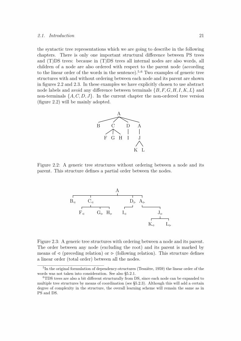
the syntactic tree representations which we are going to describe in the followingchapters. There is only one important structural difference between PS treesand (T)DS trees: because in (T)DS trees all internal nodes are also words, allchildren of a node are also ordered with respect to the parent node (accordingto the linear order of the words in the sentence).5,6 Two examples of generic treestructures with and without ordering between each node and its parent are shownin figures 2.2 and 2.3. In these examples we have explicitly chosen to use abstractnode labels and avoid any difference between terminals {B,F,G,H, I,K,L} andnon-terminals {A,C,D,J}. In the current chapter the non-ordered tree version(figure 2.2) will be mainly adopted.
A
B C
F G H
D
I
A
J
K L
Figure 2.2: A generic tree structures without ordering between a node and itsparent. This structure defines a partial order between the nodes.
A
B⪦ C⪦ D⪧ A⪧
F⪦ G⪧ H⪧ I⪦ J⪧
K⪦ L⪧
Figure 2.3: A generic tree structures with ordering between a node and its parent.The order between any node (excluding the root) and its parent is marked bymeans of ⪦ (preceding relation) or ⪧ (following relation). This structure definesa linear order (total order) between all the nodes.
5In the original formulation of dependency-structures (Tesniere, 1959) the linear order of thewords was not taken into consideration. See also §5.2.1.
6TDS trees are also a bit different structurally from DS, since each node can be expanded tomultiple tree structures by means of coordination (see §5.2.3). Although this will add a certaindegree of complexity in the structure, the overall learning scheme will remain the same as inPS and DS.

22 Chapter 2. Generalized Tree-Generating Grammars
2.2 Symbolic Generative Models for TreesA symbolic tree-generating grammar can be defined as follows:
2.2.1. Definition. A symbolic tree-generating grammar G is a tuple:
G = ⟨N ,A,⊙,⊕,⊘,⍟,m,F1, . . . , Fm,C1, . . . ,Cm,O1, . . . ,Om⟩
where N is a finite set of symbols (or nodes), A ⊂ N a set of artificial symbols,⊙ ∈ A the start symbol, ⊕ ∈ A the stop symbol, ⊘ ∈ A the null symbol, ⍟ ∈ Athe wild-card symbol, m ∈ N≥1 the number of operations allowed in the grammar,Fi (i ∈ {1, . . .m}) a finite list (or class7) of elementary fragments, Ci a finite list(or class) of conditioning contexts such that ∣Fi∣ = ∣Ci∣, and Oi a compositionaloperation that can apply only to fragments in Fi and conditioning contexts in Ci.
A generative model implementing a symbolic grammar is able to derive atree structure through a series of generative events. Each generative event mod-ifies a partially derived structure by means of a specific compositional operationintroducing a new elementary fragment. In order for the operation to apply,some specific part of the generated structure, i.e., the conditioning context, mustuniquely specify the site where the fragment is introduced. Given a model, eachfragment fi,j ∈ Fi is uniquely mapped to a specific conditioning context ci,j ∈ Ci.
2.2.1 The event spaceAn elementary fragment represents a new piece of the tree introduced by a gener-ative event. It is defined in the general case as a multiset of nodes; if empty, thecorresponding operation is a transformation8 of the current tree: no novel nodesare introduced in the structure. Figure 2.4 presents 5 examples of generally validfragments.
Every class of fragments Fi must characterize the topology of each of its mem-bers fi,j, i.e., the pairwise relations between the nodes in fi,j. When the nodesform a tree structure, the edges implicitly define these relations. In other casesthe relations need to be clearly specified. For instance the fragment (b) in figure2.4 represents a sequence of nodes which do not form a tree structure.9 Sucha list of nodes is often used (without dotted edges) in later examples to definea sequence of adjacent siblings, which will share the same parent node alreadypresent in the partially derived tree. It is important to specify that such relations
7We will generally use the term list to refer to an enumeration of elements (duplicatesallowed), while class will be used to refer to the set of the elements in the list. We have chosenthis convention to allow a unique mapping between each fi,j ∈ Fi and ci,j ∈ Ci specified by theindex j.
8For an example of a transformation see example 2.2.8 at page 36.9In order to be a tree structure the four daughters would need a parent node.

2.2. Symbolic Generative Models for Trees 23
should hold right after the operation is applied, but not necessarily after the treestructure is completed. In fact other generative events might break these rela-tions by introducing novel nodes in the structure. The class Fi can characterizeits members imposing a set of properties. For instance a fragment class mightspecify that no more than 2 nodes are allowed, or that all its fragments are trees.
⊕ B C D A
⊙
A
B
⊕
A
B C
F G H
(a) (b) (c) (d) (e)
Figure 2.4: Examples of 5 elementary fragments.
2.2.2 The conditioning contextA conditioning context (in short context) describes a part of the structure whichhas been previously generated (therefore also sometimes referred to as a history).
Differently from fragments, each context is defined as a multiset containingone or more nodes (no empty contexts are allowed) connected in a tree structure.As for Fi, a model may define for a class Ci of contexts possible constraints on thestructure, while the topology (relations between the nodes) is always implicitlydefined by the tree structure.
Figure 2.5 shows 6 possible conditioning contexts. When defining a context, amodel can introduce an arbitrary number of check conditions, which are shown inthe contexts by means of two artificial nodes: the null symbol ⊘ which representthe absence of a node, and the wild-card node ⍟ with represent the presence ofan unspecified node. For instance one could enforce that in a certain context, acertain node A does not have any daughters (figure 2.5-b); that nodes B and D aredaughters of an unspecified parent node10 (figure 2.5-c); that A is A’s rightmostdaughter (figure 2.5-d); that C and D are adjacent daughters of A, without anynode in between (figure 2.5-e); and finally that F and H are daughters of A withone unspecified daughter in between (figure 2.5-f).
10It is important to understand that in this example the context specifies that B and D aresiblings, with B preceding D, but not necessarily immediately (see difference with figure 2.5-e).

24 Chapter 2. Generalized Tree-Generating Grammars
In a model it is possible that two context tokens are equivalent, i.e., ci,j =ci,q with j ≠ q. In this case ci,j and ci,q are the same context type since theyrepresent the same structure, but different context tokens as they map to differentfragments. It is in fact assumed that grammars are not redundant, so that ci,j =ci,q → fi,j ≠ fi,q with j ≠ q.
⊙
A
⊘
⍟
B D
A
A ⊘
A
C ⊘ D
C
F ⊘ ⍟ ⊘ H
(a) (b) (c) (d) (e) (f)
Figure 2.5: Examples of 6 conditioning contexts (or histories).
2.2.3 Context-Free GrammarIn order to clarify the notation introduced so far we will now describe an exampleof Context-Free Grammar (Chomsky, 1956).
2.2.2. Example. [Context Free Grammar] According to definition 2.2.1, wehave m = 1 (one single fragment and context class and a single operation), eachf1,j ∈ F1 is a list of adjacent daughters (the right hand side of each productionrule), each c1,j ∈ C1 a single node (the corresponding left hand side of the sameproduction) such that c1,j is the parent node of the nodes in f1,j, and O1 theoperation of attaching the daughters in f1,j, to c1,j (substitution operation). Asa check condition the node in c1,j should have no daughter nodes, i.e., it must bea frontier node in the tree structure before the operation is applied. Figure 2.6(right) shows the contexts and the elementary fragments for the CFG extractedfrom the tree in figure 2.2, also reported in the left-side of the same figure forconvenience.
When using this grammar to generate a structure T , we begin with the startsymbol⊙ identifying T0 in all the models. At this point only the first conditioningcontext in the grammar (⊙ Ð ⊘) can apply, and therefore T1 is obtained byattaching A as the unique daughter node of the initial symbol. At this pointthere are 2 identical conditioning contexts which are applicable (AÐ⊘, at indicesj = 2,3), and there are therefore two possible ways of continuing the generationof a structure.11
11See also the section on multiple derivations in §2.2.4

2.2. Symbolic Generative Models for Trees 25
A
B C
F G H
D
I
A
J
K L
j C1 F 1
1 ⊙Ð⊘ A2 AÐ⊘ B C D A3 AÐ⊘ J4 CÐ⊘ F G H5 DÐ⊘ I6 JÐ⊘ K L7 BÐ⊘ ⊕8 FÐ⊘ ⊕9 GÐ⊘ ⊕
10 HÐ⊘ ⊕11 I Ð⊘ ⊕12 KÐ⊘ ⊕13 LÐ⊘ ⊕
Figure 2.6: Left: the PS tree from figure 2.2. Right: the CFG extracted from theleft tree. C1 identifies the left-hand side of the CFG rules, F1 the right-hand side.
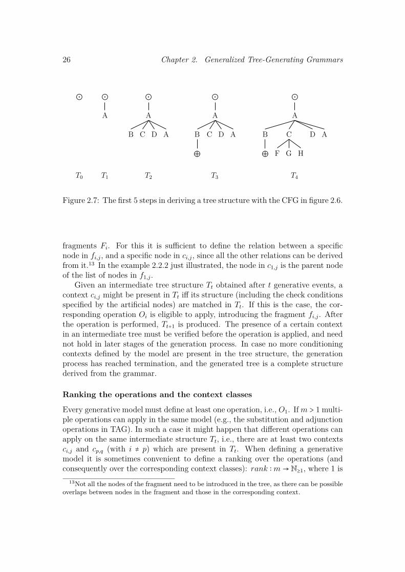
The first 4 steps of a possible derivation of this grammar are illustrated infigure 2.7. At every step the left-most non-terminal node at the frontier of theintermediate structure is the context for the following generative step.12 Thispartial derivation can be completed to return the original structure in figure 2.2.The remaining steps are shown in figure 2.8(a) using indices in nodes to refer to thestages of the derivation process in which the nodes are introduced. Figure 2.8(b)reports an alternative derivation licensed by the same grammar. According tothis grammar, a tree is complete when all the nodes at the frontier are the stopsymbol ⊕.
2.2.4 The generative processThe role of a context ci,j is essential in a generative process. If its correspondingfragment fi,j is empty, it specifies where the transformation takes place (specifiedby the operation Oi). Otherwise, it locates where the corresponding fragmentneeds to be placed within the current incomplete structure via the associatedcompositional operation Oi. In this case it is necessary to define the relationbetween each class of conditioning contexts Ci and the corresponding class of
12See also the section on locating a single context at a time in §2.2.4
26 Chapter 2. Generalized Tree-Generating Grammars
⊙ ⊙
A
⊙
A
B C D A
⊙
A
B
⊕
C D A
⊙
A
B
⊕
C
F G H
D A
T0 T1 T2 T3 T4
Figure 2.7: The first 5 steps in deriving a tree structure with the CFG in figure 2.6.
fragments Fi. For this it is sufficient to define the relation between a specificnode in fi,j, and a specific node in ci,j, since all the other relations can be derivedfrom it.13 In the example 2.2.2 just illustrated, the node in c1,j is the parent nodeof the list of nodes in f1,j.
Given an intermediate tree structure Tt obtained after t generative events, acontext ci,j might be present in Tt iff its structure (including the check conditionsspecified by the artificial nodes) are matched in Tt. If this is the case, the cor-responding operation Oi is eligible to apply, introducing the fragment fi,j. Afterthe operation is performed, Tt+1 is produced. The presence of a certain contextin an intermediate tree must be verified before the operation is applied, and neednot hold in later stages of the generation process. In case no more conditioningcontexts defined by the model are present in the tree structure, the generationprocess has reached termination, and the generated tree is a complete structurederived from the grammar.
Ranking the operations and the context classes
Every generative model must define at least one operation, i.e., O1. If m > 1 multi-ple operations can apply in the same model (e.g., the substitution and adjunctionoperations in TAG). In such a case it might happen that different operations canapply on the same intermediate structure Tt, i.e., there are at least two contextsci,j and cp,q (with i ≠ p) which are present in Tt. When defining a generativemodel it is sometimes convenient to define a ranking over the operations (andconsequently over the corresponding context classes): rank ∶m→ N≥1, where 1 is
13Not all the nodes of the fragment need to be introduced in the tree, as there can be possibleoverlaps between nodes in the fragment and those in the corresponding context.

2.2. Symbolic Generative Models for Trees 27
⊙0
A1
B2
⊕3
C2
F4
⊕5
G4
⊕6
H4
⊕7
D2
I8
⊕9
A2
J10
K11
⊕12
L11
⊕13
⊙0
A1
J2
K3
⊕4
L3
⊕5
(a) (b)
Figure 2.8: Two complete trees which can be derived from the CFG in figure 2.6.
the highest rank.14 If not specified otherwise, rank is the identity function: thefirst operation (conditioning context class) has priority over the second, whichhas priority over the third, and so on. At each stage we retain only the contexttokens present in the current tree with highest rank. If no ranking is adopted ina specific model, all the operations can apply at a given stage.
Locate a single context at a time
It can happen that at a given stage t of the generation process, a context type15 ispresent in Tt at different locations, or that two different context types are presentin Tt each at a different location. For instance in the intermediate tree T2 infigure 2.7 all four nodes B,C,D,A at the frontier of the intermediate structureare possible contexts in which O1 can apply. In general this can be problematic,as the same sequence of operations applied in different locations might result indifferent emerging structures. Therefore at every stage of the derivation processwe want to ensure that every model defines a way to deterministically locatein Tt a single context type on which to apply the corresponding compositionaloperation.
14If no rank is defined, multiple operations might apply at the same time. In the probabilisticextensions of symbolic tree-generating grammars (§2.3), we will always assume the definitionof a ranking function.
15Remember the distinction between context type and context token specified at the end of§2.2.2.

28 Chapter 2. Generalized Tree-Generating Grammars
A1
B2 C3
F4 G5 H6
D7
I8
A9
J10
B11 D12
Figure 2.9: A depth-first ordering of the nodes in a tree.
For CFGs the solution is to impose the left-most substitution to apply (asshown in the indices of figure 2.8). In the general case, we define a locationfunction L (c, Tt) returning the location of a context type c in Tt. If n = ∣c∣ isthe number of nodes in c, we define L (c, Tt)={`1(c, Tt), `2(c, Tt), . . . , `r(c, Tt)}with r ≥ 1 being the number of times c is present in Tt, and `i(c, Tt) ∈ Nn the ithlocation of c in Tt, i.e., a set of indices identifying the positions of c’s nodes in Tt.The indices of the nodes in Tt are assigned according to a pre-establish ordering,conventionally a depth-first ordering as shown in figure 2.9. To give an examplelet us consider context in figure 2.5-c, and assume that the tree in figure 2.9 isour Tt. We then have L (c, Tt) = {`1(c, Tt) = {1,2,7}, `2(c, Tt) = {10,11,12}}.
Every model must ensure that for every two context types c ≠ c′ that canapply16 in Tt there exist no i, j ∈ N≥1 such that `i(c, Tt) = `j(c′, Tt). In other words,different contexts should be always mutually exclusive, if one applies at a certainlocation in Tt the other should not be present or its location should differ, and viceversa. This is to ensure that in every model a given sequence of generative eventsproduces a unique structure. We can therefore define an ordering of the locationsof all contexts present in Tt, in order to localize a unique context at a time. IfA = `i(a,Tt) and B = `j(b, Tt), with A ≠ B, we have A < B⇔ A ⊂ B ∨ min(A ∖B) < min(B ∖ A). For example, the contexts c, d, e, f in figure 2.5 are presentin tree Tt of figure 2.9 at locations: `1(c, Tt) = {1,2,7} < `1(e, Tt) = {1,3,7} <`1(d, Tt) = {1,9} < `1(f, Tt) = {3,4,5,6} < `2(c, Tt) = {10,11,12}. Context c wouldtherefore apply.
Multiple derivations
Given that the model has successfully selected a single context type c in theintermediate tree Tt at location `i(c, Tt), for most non-trivial grammars there
16Remember that in order for c and c′ to apply, they must have the same rank.

2.2. Symbolic Generative Models for Trees 29
might be multiple context tokens instantiating c, e.g., ci,j = cp,q = c, with i ≠p ∨ j ≠ q ∧ rank(i) = rank(p). Trivially all context tokens apply at the samelocation `i(c, Tt).
When this circumstance arises, multiple distinct fragments are associated withthe same type of context, and are therefore eligible to apply. For instance inexample 2.2.2 when A is the selected context both rules A → B C D E and A →J can apply.
In this case the model must allow for all corresponding fragments to apply, butin parallel: each fragment is applied on an identical copy of the current partialtree Tt. In other words the current derivation splits in multiple derivations, one forevery distinct context tokens which applies. This generates novel derivations ofthe grammar that will potentially differ in all following steps, producing differentcomplete trees. But it can also happen that some of these derivations eventuallyproduce the same complete structure. When this occurs, the grammar is saidto have spurious ambiguities.17 Context-free grammars do not show this type ofambiguity, but TSG grammars do (see example 2.2.3 and chapter 3).
Artificial symbols
The artificial symbols thus far introduced are the symbols in the set A = {⊙,⊕,⊘,⍟}. In addition, a model can introduce an arbitrary number of artificial symbols,which usually serve as placeholders to represent specific choices which are madealong the way in the generative process. All the artificial symbols need to beremoved after the termination of the generative process in order to obtained acleaned complete structure.
The start symbol ⊙ represents the only symbol which is present in the treestructure T0, before any generation event takes place. In general, the start symbolmay be present in fragment fi,j, but only as a reference node as no operation Oi
can insert a second start symbol into the tree.The stop symbol ⊕ represents a node in the tree which signals the termination
of a specific generation sub-process, but a derivation does not necessarily need toemploy ⊕ in order to terminate.18
The null symbol ⊘ represents the absence of a certain node. It can onlybe used within contexts, typically to define specific check conditions that needto be present in the current incomplete structure for a certain context to apply(see figure 2.5).
Finally, the wild-card symbol ⍟, like ⊘, can be only used for contexts. Itmatches any possible non-artificial node (N ∖A).
17This should not be confused with the standard notion of ambiguity of the grammar, forwhich there exist multiple structures associated to the same sentence.
18As explained in §2.2.4, it is sufficient that no conditioning context is present in the derivedstructure for the generative process to terminate.

30 Chapter 2. Generalized Tree-Generating Grammars
2.2.5 Extracting a symbolic grammar from a treebankSymbolic grammars can be written manually or they can be extracted from acollection of annotated parse trees, the training treebank T . We are mainlyinterested in pursuing the second option, but in either case we have to choose whatthe model behind the grammar looks like, i.e., what its composition operationsare, and how each fragment and context class is defined. After describing theprimitives of the model, we take each structure one by one in the training treebankT and simulate how it can be derived according to the model under consideration.This procedure can be seen as a decomposition of the structure into elementaryfragments, each linked to a conditioning context. During this decomposition, weequip the grammar with the fragments and conditioning contexts pairs which areemployed. After iterating the same procedure for all the trees in T , we havederived a symbolic grammar. This in turn will be capable of deriving all the treestructures in T , and possibly many other structures which are a generalizationof the observed ones in the treebank.
2.2.6 Examples of generative tree grammarsTo demonstrate the generality of the notions just described, we will now describe6 examples of generative grammars. All the grammars are extracted from the PSin figure 2.2, except for the grammar in example 2.2.5 which is extracted fromthe DS in figure 2.3.
2.2.3. Example. [Tree-Substitution Grammar] In this example we presenta TSG grammar which employs subtrees of arbitrarily large size as fragments forthe generative operations. This formalism was first implemented in Bod (1992),and will be used in chapter 3 for phrase-structure parsing. For this grammar wechoose m = 1, f1,j ∈ F1 is a tree structure, c1,j ∈ C1 the root node of f1,j exactly asin CFG (example 2.2.2), and O1 the operation of introducing the full fragment f1,jin the tree by substituting c1,j with the root of f1,j. Figure 2.10 (a) shows a TSGgrammar which is able to derive the same tree structure as in the CFG example(§2.2.3) with two different derivations as shown in figure 2.10 (a,b). Moreover,this grammar can derive an infinite number of tree structures, and exactly thoseproduced by the previous CFG.
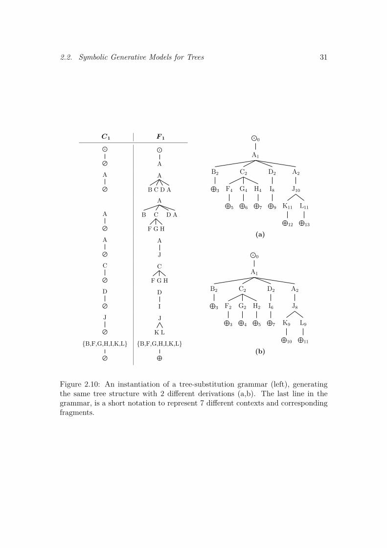
2.2. Symbolic Generative Models for Trees 31
C1 F 1
⊙
⊘⊙
AA
⊘
A
B C D A
A
⊘
A
B C
F G H
D A
A
⊘
A
JC
⊘
C
F G HD
⊘
D
IJ
⊘
J
K L
{B,F,G,H,I,K,L}
⊘
{B,F,G,H,I,K,L}
⊕
⊙0
A1
B2
⊕3
C2
F4
⊕5
G4
⊕6
H4
⊕7
D2
I8
⊕9
A2
J10
K11
⊕12
L11
⊕13
(a)
⊙0
A1
B2
⊕3
C2
F2
⊕3
G2
⊕4
H2
⊕5
D2
I6
⊕7
A2
J8
K9
⊕10
L9
⊕11
(b)
Figure 2.10: An instantiation of a tree-substitution grammar (left), generatingthe same tree structure with 2 different derivations (a,b). The last line in thegrammar, is a short notation to represent 7 different contexts and correspondingfragments.

32 Chapter 2. Generalized Tree-Generating Grammars
2.2.4. Example. [Right Sister Insertion Grammar (PS)] This grammar isa simplification of previous work (Magerman, 1995; Collins, 1996), and demon-strates that our formalisms is general enough to model rule markovization withoutrelying on a special-purpose grammar representation.
The basic operation behind this grammar is to introduce a single daughterto a node in the tree, conditioned on its parent node and its left sister. Wechoose m = 1, f1,j is a single node (the new daughter), c1,j contains the rootnode of f1,j and its right-most daughter (⊘ if no daughters are present), O1 theoperation of attaching f1,j as the new right-most daughter of the parent node inc1,j. Figure 2.11 shows this example in more detail.
C1 F 1
⊙⊘ A⊙
A ⊘ ⊕A
⊘ BA
B ⊘ CA
C ⊘ DA
D ⊘ AA
A ⊘ ⊕B
⊘ ⊕C
⊘ F
C1 F 1
C
F ⊘ GF
G ⊘ HG
H ⊘ ⊕D
⊘ ID
I ⊘ ⊕A
⊘ JF
⊘ ⊕G
⊘ ⊕
C1 F 1
H
⊘ ⊕I
⊘ ⊕J
⊘ ⊕J
K ⊘ KJ
L ⊘ LJ
⊘ ⊕K
⊘ ⊕L
⊘ ⊕
⊙0
A1
B 3 ⊕8
C4
F 9 ⊕13
G10
⊕14
H11
⊕15
⊕12
D5
I 16
⊕18
⊕17
A6
J 19
K21
⊕24
L 22
⊕25
⊕23
⊕20
⊕7
⊕2
Figure 2.11: A Right Sister Insertion Grammar (left) for PS, generating a treestructure (right) by introducing a new rightmost daughter of a node at every step.

2.2. Symbolic Generative Models for Trees 33
2.2.5. Example. [Right Sister Insertion Grammar (DS)] This grammar issimilar to the previous one except that it is adapted to the DS representation (Eis-ner, 1996b). As before a single node is introduced at each step, conditioned onits parent node and its left sister. We set m = 1, f1,j is a fragment partiallyoverlapping with the respective context, c1,j contains the root node of f1,j and itsright-most daughter (⊘ if no daughters are present), O1 the operation of attach-ing the rightmost daughter in f1,j as the new right-most daughter of the parentnode in c1,j. Left and right daughters of every node are filled in as two separateprocesses. Figure 2.12 shows this example in more detail.
C1 F 1
X
⊘
X
⊘ Z
for (X,Z) ∈ {(⊙,A),(A,B), (B,⊕),(C,F ), (D,I),(A,⊕), (F,⊕),(G,⊕), (H,⊕),(I,⊕), (J,K),(K,⊕), (L,⊕)}
X
Y
X
Y Z
for (X,Y,Z) ∈{(⊙,A,⊕),(A,B,C), (A,C,⊕),(C,F,⊕), (D,I,⊕),(J,K,⊕)}
C1 F 1
X
⊘
X
⊘ Z
for (X,Z) ∈ {(⊙,⊕),(A,D), (B,⊕),(C,G), (D,⊕),(A,J), (F,⊕),(G,⊕), (H,⊕),(I,⊕), (J,L),(K,⊕), (L,⊕)}
X
Y
X
Y Z
for (X,Y,Z) ∈{(A,D,A), (A,A,⊕),(C,G,H), (C,H,⊕),(A,J,⊕), (J,L,⊕)}
⊙0
A1⊕
2⊕
3
B4
C5
⊕6
D7
A8
⊕9
⊕10
⊕11
F12
⊕13
G14
H15
⊕16
I 17
⊕18
⊕19⊕
20J
21⊕
22
⊕23
⊕24
⊕25
⊕26⊕
27⊕
28⊕
29⊕
30K
31⊕
32L
33⊕
34
⊕35
⊕36
⊕37
⊕38
Figure 2.12: A Right Sister Insertion Grammar (left), generating the DS treestructure in figure 2.3 (right).
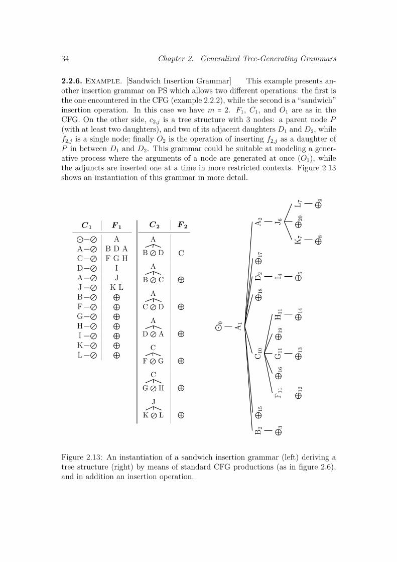
34 Chapter 2. Generalized Tree-Generating Grammars
2.2.6. Example. [Sandwich Insertion Grammar] This example presents an-other insertion grammar on PS which allows two different operations: the first isthe one encountered in the CFG (example 2.2.2), while the second is a “sandwich”insertion operation. In this case we have m = 2. F1, C1, and O1 are as in theCFG. On the other side, c2,j is a tree structure with 3 nodes: a parent node P(with at least two daughters), and two of its adjacent daughters D1 and D2, whilef2,j is a single node; finally O2 is the operation of inserting f2,j as a daughter ofP in between D1 and D2. This grammar could be suitable at modeling a gener-ative process where the arguments of a node are generated at once (O1), whilethe adjuncts are inserted one at a time in more restricted contexts. Figure 2.13shows an instantiation of this grammar in more detail.
C1 F 1
⊙Ð⊘ AAÐ⊘ B D ACÐ⊘ F G HDÐ⊘ IAÐ⊘ JJÐ⊘ K LBÐ⊘ ⊕FÐ⊘ ⊕GÐ⊘ ⊕HÐ⊘ ⊕I Ð⊘ ⊕KÐ⊘ ⊕LÐ⊘ ⊕
C2 F 2
A
B ⊘ D CA
B ⊘ C ⊕A
C ⊘ D ⊕A
D ⊘ A ⊕C
F ⊘ G ⊕C
G ⊘ H ⊕J
K ⊘ L ⊕
⊙0
A1
B 2 ⊕3
⊕15
C10
F 11
⊕12
⊕16
G11
⊕13
⊕19
H11
⊕14
⊕18
D2 I 4 ⊕5
⊕17
A2 J 6
K7
⊕8
⊕20
L 7 ⊕9
Figure 2.13: An instantiation of a sandwich insertion grammar (left) deriving atree structure (right) by means of standard CFG productions (as in figure 2.6),and in addition an insertion operation.

2.2. Symbolic Generative Models for Trees 35
2.2.7. Example. [Tree-Adjoining Grammar] In this example we describe agrammar which is based on previous work on TAGs (Joshi, 1985; Joshi and Sch-abes, 1991). In this case we have m = 2. F1, C1, and O1 are as in the CFGdescribed before. O2 is an operation which allows to adjoin a full subtree f2,j ata specific site of the current tree according to the location of c2,j (a single nodehaving at least one daughter node). Each fragment in F2 is such that one of itsfrontier nodes should have the same label as its root node X; since multiple Xcan be present at the frontier, we will mark one as X* (the foot node). The oper-ation O2 excises the subtree rooted in c2,j from the tree, and puts in its place f2,j.Moreover the excised subtree is substituted to the foot node. Both the root nodeX and the foot X* cannot be used as locations for other adjunction operations.To ensure this, the two node are marked as X (this could be achieved also byadding special purpose artificial nodes, but we have chosen a shorter notation forsimplicity). Figure 2.14 presents an instance of this grammar.
C1 F 1
⊙Ð⊘ AAÐ⊘ JDÐ⊘ IJÐ⊘ K LBÐ⊘ ⊕FÐ⊘ ⊕GÐ⊘ ⊕HÐ⊘ ⊕I Ð⊘ ⊕KÐ⊘ ⊕LÐ⊘ ⊕
C2 F 2
A
⍟
A
B C
F G H
D A*
⊙0
A1
J2
K3
⊕4
L3
⊕5
⊙0
A6
B6 C6
F6 G6 H6
D6 A1
J2
K3
⊕4
L3
⊕5
⊙0
A6
B6
⊕7
C6
F6
⊕8
G6
⊕9
H6
⊕10
D6
I11
⊕12
A1
J2
K3
⊕4
L3
⊕5
(a) (b) (c)
Figure 2.14: An example of a tree-adjoining grammar (above), and one of itsderivations (below): after 5 steps (a), after 6 steps (b), after completion (c).
36 Chapter 2. Generalized Tree-Generating Grammars
2.2.8. Example. [Bottom-Up Grammar] The last example is inspired by thework of Ratnaparkhi (1997). Similar ideas are described in shift-reduced ap-proaches such as in Aho and Johnson (1974), and Shieber (1983). This exampledemonstrates that our formalism is general enough to model a wide range ofgenerative models including those based on a bottom-up generation process.
According to this generative model, structures are generated starting from theleaf-nodes, and going upwards until reaching the root of the tree. One way to dothis is to introduce internal nodes, level after level.
A bottom-up grammar is described as follows: m = 3, O1 is the operationwhich adds each leaf node of the tree structure (represented by f1,j), as the lastdaughter of the starting node given its current rightmost leaf (c1,j). The second(O2) and third operation (O3) have the same context which have equal priorities:c2,j = c3,j is found in the current tree when the right-most leaf Y of the startingnode, immediately following X, is completed (it contains the stop symbol ⊕ asits rightmost daughter).
If context c2,j is present in the current tree, and O2 is applied, the operation‘opens’ a new constituent, i.e., it inserts a new node (Z = f2) as the parent of Yand the right-sister of X. This operation is explicitly marked with a new artificialnode↗, inserted in between Z and Y . In addition↗ is followed by a new artificialsymbol → to indicate that the newly open constituent Z needs at least one otherdaughter, or alternatively by ⊕ to indicate that it is completed.
If context c3,j is present and O3 is applied, a transformation takes place: Yis attached as the new rightmost daughter of X. This operation is explicitlymarked with a new artificial node ↑, inserted in between X and Y . In addition↑ is followed by a new artificial symbol → to indicate that X needs at least oneother daughter, or alternatively by ⊕ to indicate that it is completed.
Figure 2.15 instantiates a bottom-up grammar which can derive the tree infigure 2.2. In the derivation process, O1 is used in steps 1-8; in the remainingcases, O2 is used when ↗ is inserted (in steps 9,10,14,16,18), and O3 is used when↑ is inserted (in steps 11,12,13,15,17,19).

2.2. Symbolic Generative Models for Trees 37
C1 F 1 O1
⊙⊘
B⊕
⊙B
⊙X ⊘
Y
⊕⊙
X Y
for (X,Y ) ∈{(B,F ), (F,G),(G,H), (H,I),(I,K), (K,L)}
⊙L ⊘ ⊕
⊙L ⊕
C2 F 2 O2
⊙X Y
⊕ ⊘⊘
Z
⊙X Z
↗Y
⊕
→
for (X,Y,Z) ∈{(⊘,B,A), (A,F,C), (A,K,J)}
⊙X Y
⊕ ⊘⊘
Z
⊙X Z
↗Y
⊕
⊕
for (X,Y,Z) ∈ {(A, I,D), (A,J,A)}
C3 O3
⊙X Y
⊕ ⊘⊘
⊙X
↑Y
⊕
→
for (X,Y ) ∈{(C,G), (A,C), (A,D)}
⊙X Y
⊕ ⊘⊘
⊙X
↑Y
⊕
⊕
for (X,Y ) ∈{(C,H), (J,L), (A,A)}
⊙0
A9
↗9
B1
⊕1
→9 ↑13
C10
↗10
F2
⊕2
→10 ↑11
G3
⊕3
→11 ↑12
H4
⊕4
⊕12
→13 ↑15
D14
↗14
I5
⊕5
⊕14
→15 ↑19
A18
↗18
J16
↗16
K6
⊕6
→16 ↑17
L7
⊕7
⊕17
⊕18
⊕19
⊕8
Figure 2.15: A bottom-up grammar (left) and one of its derivation. All the nodesin the structure are introduced one level at a time.

38 Chapter 2. Generalized Tree-Generating Grammars
2.3 Probabilistic Generative Models for TreesThe symbolic formalism developed so far allows for a straightforward probabilisticextension. For simplicity we assume that the underlying symbolic model alwaysdefines a ranking function over the operations (when multiple are present). Thisensures that there is a unique operation which applies at a given stage of thederivation process (see 2.2.4). A probabilistic tree-generating grammar is definedas follows:
2.3.1. Definition. A probabilistic tree-generating grammar Gp extends the def-inition 2.2.1 of a symbolic tree-generating grammar with a function p(fi,j ∣ci,j),which returns the probability of a generative event, i.e., employing a fragmentfi,j in an intermediate tree where context ci,j applies, by means of operation Oi.The two indices i, j are such that 1 ≤ i ≤m and 1 ≤ j ≤ ∣Fi∣ = ∣Ci∣. The index i willbe always fixed as it specifies the operation which is deterministically selected bythe rank according to the symbolic model. We maintain this index in order to beconsistent with the previous notation of the underlying symbolic grammar (§2.2).
The function p must correspond to a proper probability distribution over thefragments sharing the same conditioning context type. This means that for everyi, j the following equation should be satisfied:
∑q s.t.
ci,j=ci,q
p(fi,q ∣ci,j) = 1 (2.6)
2.3.1 Resolving the syntactic ambiguityAs mentioned in §2.1.1 a symbolic generative grammar can be extended with astochastic component to resolve cases of syntactic ambiguities. In fact, for anynon-trivial symbolic grammar, there are many possible tree structures yielding agiven sentence s. We therefore need to define a way to induce probabilities overthe trees generated from the grammar whose yield is s, and select the one withmaximum probability. This is equivalent to say that we want to obtain the parsetree T such that:
T = arg maxT
p(T ∣s) (2.7)
= arg maxT
p(T, s)P (s) (2.8)
= arg maxT
p(T, s) (2.9)

2.3. Probabilistic Generative Models for Trees 39
2.3.2 The probability of a treeGiven a probabilistic tree-generating grammar Gp, and a tree structure T it cangenerate, we want to obtain P (T ∣Gp): the probability of T according to Gp. Inthe following explanation we assume an underlying probabilistic grammar Gp andwe therefore use the simpler notation P (T ).
We start by decomposing T into a sequence of independent generative events,forming the first derivation of T : δ1(T ) = (e1, e2, . . . , en) producing a sequence ofintermediate structures (T1, T2, . . . , Tn−1) and terminates with the complete treeTn = T . Each event e = ⟨fi,j, ci,j⟩ is characterized by an elementary fragmentfi,j and a corresponding conditioning context ci,j which are present in Gp. Theprobability of each event p(e) is given by the function p(fi,j ∣ci,j) introduced before(in definition 2.3.1).
Since the generative events are defined to be independent, we can computethe probability of a derivation by multiplying the probabilities of its events.
P (δi(T )) = ∏e∈δi(T )
p(e) = ∏e∈δi(T )
p(e) (2.10)
If the model generates m different derivations for T , we obtain them all, i.e.,D(T ) = {δ1(T ), δ2(T ), . . . , δm(T )}. The probability of T is then obtained bysumming the probabilities of all possible derivations in D(T ):
P (T ) = ∑δi∈D(T )
δi(T ) = ∑δi∈D(T )
∏e∈δi(T )
p(e) (2.11)
2.3.3 Estimating Probability DistributionsThe function p in definition 2.3.1 is the only function needed to characterizea probabilistic tree-generating grammar. The possible choices for p (satisfyingequation 2.6) are unlimited, and there is not a single one which is “correct” inany principled way. Nevertheless, choosing a probability distribution at random isalso not a recommended strategy. More viable solutions are obtained by definingspecific heuristics to guide the choice. Alternatively it is possible to define anindependent objective function and find the distribution p which maximizes it.Again there is not a single heuristic or objective function which is more correct.A standard way to compare these strategies is by analyzing their differences basedon empirical testing.
Following different guiding strategies, we will now introduce two well stud-ied probability estimates to infer p: the Relative Frequency Estimate, and theMaximum Likelihood Estimate. Finally, we also discuss an alternative generalmethodology to induce a probabilistic grammar Gp: Bayesian Inference.

40 Chapter 2. Generalized Tree-Generating Grammars
Relative Frequency Estimate
The Relative Frequency Estimate (RFE) is the simplest heuristic to derive aprobability distribution pRFE over the fragments. It is widely used in statisticalmodels, as for many formalisms there are theoretical and empirical proves of itsstability. RFE makes use of two count functions ⟨countf , countc⟩, which corre-spond to the frequencies with which fragments and contexts occur in deriving thetree structures in the training treebank T :countf(fi,j) : returns the frequency of fragment token fi,j in T , when occurring
in context ci,j.
countc(ci,j) : returns the frequency of context types ci,j in T .While countf is defined over fragment tokens, countc is defined over context types.This implies that for any j and q such that ci,j = ci,q the following equation shouldhold:
countc(ci,j) = countc(ci,q) (2.12)Moreover, the sum of the counts of all fragments sharing the same context typemust equal the count of that context:
∑q s.t.
ci,j=ci,q
countf(fi,q) = countc(ci,j) (2.13)
The probability pRFE is defined following the intuition that a fragment fi,jmust be used in a certain context ci,j proportionally to the fraction of times ithas been extracted in that context:
pRFE(fi,j ∣ci,j) =countf(fi,j)countc(ci,j)
(2.14)
This estimate infers a proper probability distribution. In fact for every jequation 2.6 is satisfied:
∑q s.t.
ci,q=ci,j
p(fi,q ∣ci,q) = ∑q s.t.
ci,q=ci,j
countf(fi,q)countc(ci,q)
(2.15)
= 1countc(ci,j)
⋅ ∑q s.t.
ci,q=ci,j
countf(fi,q) (2.16)
= countc(ci,j)countc(ci,j)
(2.17)
= 1 (2.18)where equation 2.16 is derived from equation 2.12, and 2.16 from 2.13.
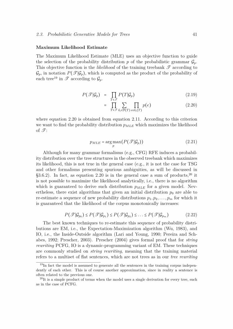
2.3. Probabilistic Generative Models for Trees 41
Maximum Likelihood Estimate
The Maximum Likelihood Estimate (MLE) uses an objective function to guidethe selection of the probability distribution p of the probabilistic grammar Gp.This objective function is the likelihood of the training treebank T according toGp, in notation P (T ∣Gp), which is computed as the product of the probability ofeach tree19 in T according to Gp.
P (T ∣Gp) = ∏T ∈T
P (T ∣Gp) (2.19)
= ∏T ∈T
∑δi∈D(T )
∏e∈δi(T )
p(e) (2.20)
where equation 2.20 is obtained from equation 2.11. According to this criterionwe want to find the probability distribution pMLE which maximizes the likelihoodof T :
pMLE = arg maxp
(P (T ∣Gp)) (2.21)
Although for many grammar formalisms (e.g., CFG) RFE induces a probabil-ity distribution over the tree structures in the observed treebank which maximizesits likelihood, this is not true in the general case (e.g., it is not the case for TSGand other formalisms presenting spurious ambiguities, as will be discussed in§3.6.2). In fact, as equation 2.20 is in the general case a sum of products,20 itis not possible to maximize the likelihood analytically, i.e., there is no algorithmwhich is guaranteed to derive such distribution pMLE for a given model. Nev-ertheless, there exist algorithms that given an initial distribution p0 are able tore-estimate a sequence of new probability distributions p1, p2, . . . , pm for which itis guaranteed that the likelihood of the corpus monotonically increases:
P (T ∣Gp0) ≤ P (T ∣Gp1) ≤ P (T ∣Gp2) ≤ . . . ≤ P (T ∣Gpm) (2.22)The best known techniques to re-estimate this sequence of probability distri-
butions are EM, i.e., the Expectation-Maximization algorithm (Wu, 1983), andIO, i.e., the Inside-Outside algorithm (Lari and Young, 1990; Pereira and Sch-abes, 1992; Prescher, 2003). Prescher (2004) gives formal proof that for stringrewriting PCFG, IO is a dynamic-programming variant of EM. These techniquesare commonly studied on string rewriting, meaning that the training materialrefers to a multiset of flat sentences, which are not trees as in our tree rewriting
19In fact the model is assumed to generate all the sentences in the training corpus indepen-dently of each other. This is of course another approximation, since in reality a sentence isoften related to the previous one.
20It is a simple product of terms when the model uses a single derivation for every tree, suchas in the case of PCFG.
42 Chapter 2. Generalized Tree-Generating Grammars
case.21 In string rewriting PCFG, MLE aims at maximizing the likelihood ofthe training sentences when varying the probabilities of the CFG rules. Thereis a striking parallelism between the two approaches; in fact, in MLE for stringrewriting PCFG, there are multiple CFG derivations for every training sentence,while in our general case there are multiple derivations for every tree in T . Wewill discuss in more detail one instance of MLE for TSG in §3.6.2.
Bayesian Inference
Bayesian Inference is a framework that derives its methodology from Bayes’ rule.
P (Gp∣T ) = P (Gp,T )P (T ) (2.23)
= P (T ∣Gp)P (Gp)P (T ) (2.24)
= P (T ∣Gp)P (Gp)∑G′p P (T ∣G′p)P (G′p)
(2.25)
In the last two equations, P (T ∣Gp) is the likelihood, the one defined in theprevious section, while P (Gp) is called the prior and specifies how good a chosenprobabilistic grammar is, before having observed any data.
In Bayesian inference we are often interested in obtaining the maximum aposteriori distribution GMAP
p which is defined as:
GMAPp = arg max
Gp
P (Gp∣T ) (2.26)
= arg maxGp
P (T ∣Gp)P (Gp)∑G′p P (T ∣G′p)P (G′p)
(2.27)
= arg maxGp
P (T ∣Gp)P (Gp) (2.28)
Goldwater et al. (2009) claim that unconstrained maximum-likelihood estima-tion is a poor way to choose among probabilistic grammars, and that Bayesianinference provides a more principled approach. In Bayesian modeling, the effectof the likelihood is counter-balanced by choosing a prior distribution that favorsfor instance simpler grammars. In this case the posterior probability can be seenas a compromise between the likelihood and the simplicity of the grammar, pro-ducing a probabilistic grammar which will adequately fit the training data whileavoiding over-fitting; in addition the chosen hypothesis will tend to generalizemore successfully to novel data.
21Similarly to our approach, treebank-based MLE is used in Prescher (2005a) and Petrov(2009).

2.4. Parsing through Reranking 43
Previous work describes how to approximate GMAPp for different formalisms (see
Johnson et al., 2007a; Post and Gildea, 2009; O’Donnell et al., 2009; Cohn et al.,2009, 2010). The difference between our approach and these models is that inour approach we always build a probabilistic instantiation on top of a symbolicgrammar, while (the mentioned) Bayesian models do not separate the two pro-cesses. This can be in general considered a point of strength of the methodology,since the two processes are bound together using a single objective function. Onthe other hand, like EM, this methodology uses approximate techniques to find asequence of grammars that increase in a posteriori probability. These approxima-tions often rely on sampling over the symbolic space. For this reason, we believethat for models having a large symbolic event space (for instance TSG) thesesampling techniques will have difficulties reaching an optimal grammars.
2.4 Parsing through RerankingGiven a probabilistic tree-generating grammar Gp, a naive way to find the mostprobable candidate structure for a given sentence (which maximizes the functionin equation 2.9) is to implement the following three steps:
1. Enumerate all possible trees yielding s according to Gp.
2. For every tree T yielding s compute its probability according to Gp.
3. Select the tree with maximum probability.
The naiveness of this approach is located in step 1. In fact, in commonly usedgenerative grammars, the number of trees yielding a certain sentence s growsexponentially with the number of words in s, so it is impossible to list all possibleparses for long sentences. The most elegant solution to this problem is to relyon an efficient parser, which uses a compact representation of the possible treesin the grammar (the parse forest) and efficiently select the most probable one.The main drawback of this approach is that the parser needs to be specific to themodel. Moreover for certain models it is not guaranteed that the most probabletree can be derived efficiently, i.e., in polynomial time (see also Sima’an, 1996,and §3.6.3).
Alternatively it is possible to restrict the search space by considering only asubset of trees yielding s, and to select the one with maximum probability. This isthe approach followed in the reranking methodology that will be now introduced.
Given a probabilistic grammar, the reranking methodology aims at calculatingthe probability the grammar assigns to a given subset of k different tree structuresthat yield the same sentence. Such a methodology is able to approximate whata parser implementing the exact same probabilistic grammar would output whenpresented with the same test sentence. In fact, the chosen structure will tend to

44 Chapter 2. Generalized Tree-Generating Grammars
match the best analysis obtained with the parser, as the number k of alternativesincreases. For this reason we can consider a reranking system a parser simulator.
The main shortcoming of a reranking methodology is that it relies on a sep-arate parser to obtain k-best candidates for every test sentence. We will refer tothis step as the first phase of the reranking procedure. The parser does not needto be extremely accurate. Ideally, one should let the parser draw structures of agiven sentence from a uniform distribution over the space of all possible struc-tures yielding the sentence. This requirement will be relaxed for practical reasonof keeping k reasonably small.
One important thing to emphasize is the two-way relation that exists betweendecomposing a given structure into elementary fragments and recomposing themto generate the same structure. This fact is essential for understanding that areranking framework is in fact conceptually identical to the process of extractingfragments and conditioning contexts from the training treebank. In other words,in the reranking framework we compute the probability of an unobserved structureby decomposing it into elementary fragments and simulating the reversed processof recomposing them into the original structure.
2.5 Discriminative and Generative modelsGenerative models of language have characterized earlier approaches in computa-tional linguistics. In more recent times, another class of models, namely discrim-inative models, has been widely employed in the field. The difference betweendiscriminative and generative models has been exhaustively discussed on boththeoretical and empirical grounds (Vapnik, 1998; Ng and Jordan, 2001; Xue andTitterington, 2008).
In parsing, the distinction lies in the way the model generalizes from theobserved annotated sentences in order to obtain the best structures for a novelsentence. A discriminative model conceives each possible structure of a given sen-tence as a multitude of features. A feature is generally defined as a binary-valuedfunction, signaling its absence or presence in a given structure. A discriminativemodel is able to learn from a training treebank, by means of a machine learn-ing classifier. This refers to a family of powerful statistical tools that learn theimportance of every feature, or feature combination present in a candidate struc-ture, to judge its level of correctness. A trained classifier is then able to assigna score to every candidate according to the features it contains. In the majorityof the implemented discriminative parsers, a machine learning classifier can beemployed in a full chart based implementation, where for every test sentence theentire set of possible tree structures is inspected, and allows the one with highestscore to be efficiently selected. For instance Collins and Roark (2004), make use ofthe perceptron algorithm (Rosenblatt, 1958) on the full phrase-structure parsingforest, and McDonald (2006) employs a Support Vector Machine Classifier (Boser

2.5. Discriminative and Generative models 45
et al., 1992) for dependency parsing.22
A generative approach, in contrast, attempts to model the process of generat-ing the structure underlying a sentence, starting from a given set of building ele-ments and compositional operations (as described in this chapter). In this thesiswe will only focus on generative models as we are mainly interested in simulatingthe full process behind the emergence of a sentence together with its underly-ing structure according to a given model. This process offers the opportunity tobetter investigate linguistic hypotheses on the generation of tree structures.
The use of reranking methodology in combination with a machine learningclassifier is often referred to as discriminative reranking. As in our generativereranking approach, a discriminative reranker makes use of another parser in thefirst phase to produce the k-best candidates for each sentence to parse. This typeof approach is common in computational linguistics, although it has been mostlyexplored for PS parsing (Collins, 2000; Collins and Duffy, 2002; Shen et al., 2003;Daume III and Marcu, 2004; Collins and Koo, 2005; Charniak and Johnson, 2005;McClosky et al., 2006; Huang, 2008; Fraser et al., 2009; Johnson and Ural, 2010).There are few other studies adopting reranking on other representations (Hallet al., 2007; White and Rajkumar, 2009) and other CL tasks (Shen et al., 2004;Dinarelli et al., 2009).
All these systems differ substantially from the reranking methodology intro-duced in §2.4: besides being discriminative models, they differ in the trainingphase: for each training sentence, they are presented with the gold structuretogether with the set of k-best candidates the support parser provides for thesame sentence (including other relevant information serving as extra-features,e.g., position in the k-best list, probability). In this way discriminative parsersare able to learn how to “draw a line” between correct and incorrect decisionsof the first-phase parser, keeping the good choices of the parser, while repairingits mistakes. In our approach, instead, reranking is seen as a way to mimick thegenerative process behind the model, and therefore in the training phase only thegold structures are provided as input to the system.
To summarize the different approaches illustrated so far, and to place in con-text the contribution of this thesis, Table 2.1 shows how the main parsing modelsin the CL literature are situated with respect to the learning approach (discrim-inative, generative), the syntactic representation (PS, DS, TDS), and the searchspace (chart based, reranking).
22The description of machine learning classifiers and discriminative models in general is be-yond the scope of this thesis. A more complete discussion on this topic is presented in Smith(2011).

46 Chapter 2. Generalized Tree-Generating Grammars
Discrim
inativeG
enerativePS
DS
PSD
ST
DS
Chart
BasedC
ollinsand
Roark
(2004)
Yamada
andM
atsumoto
(2003);Nivre
(2003);M
cDonald
(2006);Hallet
al.(2006)
Bod(1993);
Collins
(1996,1997);C
harniak(1996);
Matsuzakiet
al.(2005);Petrov
etal.(2006);thisw
ork(ch.
3)
Eisner(1996a,b)
Reranking
Collins
(2000);C
ollinsand
Duffy
(2002);C
harniakand
Johnson(2005)
Hallet
al.(2007)Bod
(2003) †;Borensztajn
andZuidem
a(2011)
thisw
ork(ch.4)
thisw
ork(ch.5)
Table2.1:C
omparison
ofthem
ainparsing
modelsin
theC
Lliterature
inrelation
tothe
currentwork,with
respecttothe
learningapproach
(discriminative,generative),the
syntacticrepresentation
(PS,DS,T
DS),and
thesearch
space(chart
based,reranking).†Bod
makes
useofreranking
when
selectingthe
shortestderivation
fromthe
km
ostprobable
parses.
2.6. Conclusions 47
2.6 ConclusionsIn this chapter we have presented a unified formalism for describing probabilisticgenerative models of syntactic tree structures. This approach has allowed us toillustrate a number of known models for parsing syntactic structures within boththe phrase-structure and dependency-structure representation, as well as easilydefining new ones (e.g., the “Sandwich Insertion Grammar” in example 2.2.6).
This general methodology will allow us to experiment with a number of vari-ous generative models of dependency-structure in chapter 4 which are evaluatedthrough the reranking procedure (illustrated in §2.4) as well as defining a com-pletely new generative model for a new tree structure representation (TDS) inchapter 5.
In the following chapter we introduce a novel Data-Oriented Parsing modelfor phrase-structure, an instantiation of the TSG example 2.2.3 (p. 30).


Though a tree grows so high,the falling leaves return to the root.
Malay proverb
Chapter 3Recycling Phrase-Structure Constructions
49
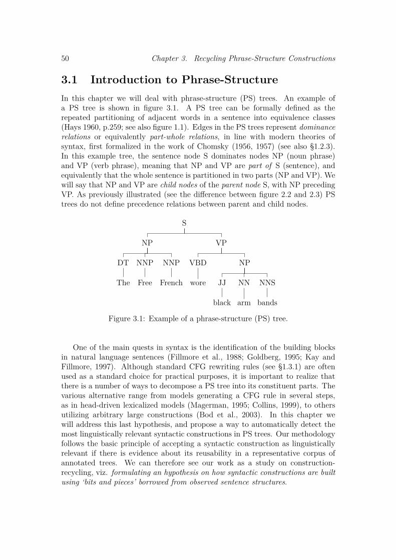
50 Chapter 3. Recycling Phrase-Structure Constructions
3.1 Introduction to Phrase-StructureIn this chapter we will deal with phrase-structure (PS) trees. An example ofa PS tree is shown in figure 3.1. A PS tree can be formally defined as therepeated partitioning of adjacent words in a sentence into equivalence classes(Hays 1960, p.259; see also figure 1.1). Edges in the PS trees represent dominancerelations or equivalently part-whole relations, in line with modern theories ofsyntax, first formalized in the work of Chomsky (1956, 1957) (see also §1.2.3).In this example tree, the sentence node S dominates nodes NP (noun phrase)and VP (verb phrase), meaning that NP and VP are part of S (sentence), andequivalently that the whole sentence is partitioned in two parts (NP and VP). Wewill say that NP and VP are child nodes of the parent node S, with NP precedingVP. As previously illustrated (see the difference between figure 2.2 and 2.3) PStrees do not define precedence relations between parent and child nodes.
S
NP
DT
The
NNP
Free
NNP
French
VP
VBD
wore
NP
JJ
black
NN
arm
NNS
bands
Figure 3.1: Example of a phrase-structure (PS) tree.
One of the main quests in syntax is the identification of the building blocksin natural language sentences (Fillmore et al., 1988; Goldberg, 1995; Kay andFillmore, 1997). Although standard CFG rewriting rules (see §1.3.1) are oftenused as a standard choice for practical purposes, it is important to realize thatthere is a number of ways to decompose a PS tree into its constituent parts. Thevarious alternative range from models generating a CFG rule in several steps,as in head-driven lexicalized models (Magerman, 1995; Collins, 1999), to othersutilizing arbitrary large constructions (Bod et al., 2003). In this chapter wewill address this last hypothesis, and propose a way to automatically detect themost linguistically relevant syntactic constructions in PS trees. Our methodologyfollows the basic principle of accepting a syntactic construction as linguisticallyrelevant if there is evidence about its reusability in a representative corpus ofannotated trees. We can therefore see our work as a study on construction-recycling, viz. formulating an hypothesis on how syntactic constructions are builtusing ‘bits and pieces’ borrowed from observed sentence structures.

3.2. Review of existing PS models 51
In the following section we will review previously proposed PS models whichare related to our work. Afterwards we will describe our main contributions:first we will present the methodology to efficiently extract reusable constructionsfrom large PS treebanks, and provide qualitative analysis of their features. Sec-ondly, we will present a Data-Oriented Parsing model (Bod et al., 2003) usingthe extracted constructions for parsing.
3.2 Review of existing PS modelsIn §1.3.1 and §2.2.3 we have introduced the Probabilistic Context-Free Grammarformalism (PCFG), which represent one of the most basic models for constructingPS trees. As explained in §1.3.2, such grammars impose heavy limitations, as theysuffer from both under-generation and over-generation problems. In the pastdecades novel probabilistic extenstions of CFGs were proposed to overcome suchlimitations. In the following sections we will review some of the most successfulmodels.
3.2.1 Head-driven modelsOne of the main innovation in PS parsing was the employment of head infor-mation to impose lexicalized conditioning on parsing decisions. The head of aphrasal constituent is a central concept in most current grammatical theories(Zwicky, 1985; Hudson, 1987; Corbett et al., 2006) and many syntax-based NLPtechniques (e.g., Magerman, 1995; Collins, 1999). The term is used to mark,for any nonterminal node in a PS tree, the specific daughter node that fulfills aspecial role. Figure 3.2 shows the tree in figure 3.1 with extra head labels (-H).
S(wore)
NP(French)
DT(The)
The
NNP(Free)
Free
NNP-H(French)
French
VP-H(wore)
VBD-H(wore)
wore
NP(bands)
JJ(black)
black
NN(arm)
arm
NNS-H(bands)
bands
Figure 3.2: Head enrichment (-H) of the tree structure in figure 3.1, and perco-lation of lexical information (in parenthesis).
As shown in the same figure, internal nodes of the PS tree can be enrichedwith lexical information which percolates up from the leaves following head an-
52 Chapter 3. Recycling Phrase-Structure Constructions
notations. Head-enrichment is usually done through compact heuristic tables asinitially proposed by Magerman (1994, 1995). Similar heuristics are used in stateof the art head-driven parses (Collins, 1997, 1999; Charniak, 1997).
Collins’ models
Collins (1997, 1999) developed three generative parsing models, based on headlexicalization techniques initially proposed by Magerman (1995). Head lexical-ization, as introduced above, consists of enriching the internal nodes of a treewith lexical information based on head annotation. This serves to constrain thelexical content on which the probability of a production should depend on, andis therefore fundamental to preventing the over-generation problems of standardPCFG models. The success of Collins’ models can be ascribed to the combinationof two further innovative techniques: rule factorization, and back-off probabilitysmoothing techniques.
Rule factorization refers to the technique of generating a parse tree attachingone daughter of a node at a time (horizontal markovization). More specifically,the head daughter is generated first, conditioned on the parent node; afterwardsleft and right siblings are produced conditioned on the head sibling, the parentnode, and a certain number of previously generated daughters.1 This is similarto the model illustrated in example 2.2.4, where each CFG production rule isfactorized in several steps according to an nth order markovian assumption. Sofor instance if we want to compute the probability to generate the top rule S(wore)→ NP(French) VP(wore) of the tree in figure 3.2, with n = 1 we will have:
head daughter Ph(V P (wore)∣S,wore) ×first left sibling Pl(NP (French)∣S,V P,wore,⊘) ×no more left siblings Pl(⊕ ∣S,V P,wore,NP (French)) ×no more right siblings Pr(⊕ ∣S,V P,wore,⊘)
where ⊘ is the null symbol and ⊕ the stop symbol as defined in 2.2. Rulefactorization is very effective to solve the under-generation problems of standardPCFG models, as the new model is capable of producing CFG rules not observedin the training set.
Back-off probability smoothing techniques are used in order to reduce com-plex probabilistic events estimations involving a large number of elements in theconditioning context (as above), to a sequence of more simple and general for-mulas. This is done in order to handle a great number of cases in which thecomplex events were not observed in the training corpus. For instance if we
1Collins introduces other elements in the conditioning context, such as a notion of distancebetween a node and the head sibling (model 1), whether a node is an argument or an adjunction(model 2), gaps for expression involving wh-movement (model 3). These advanced features arenot illustrated here for simplicity reasons.

3.2. Review of existing PS models 53
have a probabilistic model estimating event e given conditioning context c asP (e∣c) = P (A∣BCDE) we could simplify it imposing 3 backing-off levels (l1, l2,l3) in which we ignore an increasingly big number of elements in the conditioningcontext, e.g., we might choose to ignore B and D first, and C in a second step:
l1 = P (A∣BCDE)l2 = P (A∣CE)l3 = P (A∣E)
The three distributions are estimated via relative frequency from the training cor-pus and then interpolated to obtain a smoothed probability estimation: P (e∣c) =λ1l1 + (1−λ1)(λ2l2 + (1−λ2)l3), with λi chosen empirically to maximize accuracy,imposing 0 ≤ λi ≤ 1. This smoothing technique is also refer to as deleted interpo-lation (for more details see also Eisner 1996a; Bikel 2004a and Appendix B).
Charniak’s models
The model in Charniak (1997) is similar to Collins (1997, 1999) except thatit uses slightly different generative models. In particular the generation of aconstituent is decomposed in two parts: initially the lexical head of the constituentis determined based on the dependency relations with its parent node; as a secondstep, non-lexicalized part of a rule is predicted (the category of the constituenttogether with its CFG expansion) conditioned on the parent node and its head-word. Moreover, the implementation of deleted estimation makes use of statisticsover clustering of words instead of single words. A more advanced parser ispresented in Charniak (1999). The model is still generative, and conceptuallysimilar to the previous model. The main difference is in the definition of a muchlarger set of features in the history of each generative event, and the use of a modelinspired by the maximum-entropy framework (Berger et al., 1996; Ratnaparkhi,1999), which makes it more robust and easier to train.
3.2.2 State-Splitting ModelsWith state-splitting approaches we refer to recent techniques (Matsuzaki et al.,2005; Prescher, 2005b; Petrov et al., 2006; Petrov, 2009) which automatically re-fine standard PCFG by introducing new artificial rules obtained by splitting eachinternal category A to a certain number of artificial subcategories A1,A2, . . . ,An,and estimating a new probability distribution over trees. In a broad sense, othernode-enrichment techniques (Goodman, 1997; Johnson, 1998; Klein and Man-ning, 2003) can be also considered as instances of state splitting models, becauseeach node in every tree is split into more refined categories based on contex-tual features (e.g., head, parent information). Nevertheless we would like hereto draw some separation between the two approaches. In fact, recent state-splitting models strongly rely on automatic methods of enrichment rather than

54 Chapter 3. Recycling Phrase-Structure Constructions
using manual annotations or pre-defined contextual features. The other impor-tant difference is that while in manual or feature-based enrichment models eachparse tree is mapped into a specific enriched structure, in state-splitting models,such as Petrov (2009), each parse tree is mapped to multiple enriched structures.As a result, the probability of a given parse tree for a test sentence is the sumof the probabilities of all the refined structures allowed by the grammar for thatparse tree. As we will see it in the later section, this characteristic is shared withData-Oriented Parsing Models.
Although there exist a number of automatically induced state-splitting mod-els, we will only present the work of Petrov (2009) as it is methodologically simpler(with respect to e.g., Matsuzaki et al., 2005) and the one achieving better results.
Berkeley parser
Petrov (2009) developed a fast and accurate parser based on state-splitting. Thelearning of the refined grammar is done automatically and incrementally, alter-nating splitting and merging phases. In a split phase every category is forked intwo subcategories and a re-estimation of the probabilities of rules is performed inorder to maximize the probability of the training corpus using the Expectation-Maximization algorithm. In the merge phase, the model checks to which extenteach splitting contributes to increase the likelihood of the data; a certain splittingis undone if its contribution is found to be negligible. Figure 3.3 shows the treein figure 3.1 with the refined categories after the 6th iteration of the Berkeleymodel.
The use of refined categories effectively helps the model in solving the over-generation problem of the underlying PCFG, as it imposes stronger constraintson the possible ways of extending each internal node of a parse tree. Theunder-generation problem is solved by using artificial binarization of the treebank(marked in the tree in figure 3.3 with ‘@’), which is a way to implicitly encodehorizontal markovization in the model as in Collins (1997, 1999) (see also §3.7).
3.3 Data-Oriented ParsingIn this section we present a novel approach to Data-Oriented Parsing (DOP).As in previous DOP models (Bod, 2001b; Bansal and Klein, 2010), our parserutilizes syntactic fragments of arbitrary size from a treebank to analyze new sen-tences. As the number of fragments which can be extracted from a large treebankis extremely large, previous approaches have resorted to explicitly extracting arandom sample of fragments (e.g., Bod, 2001b), or implicitly representing themall in a compact grammar (e.g., Bansal and Klein, 2010).
The main contribution of our work is to propose a more principled-basedapproach for explicitly extracting a relatively small but representative set of
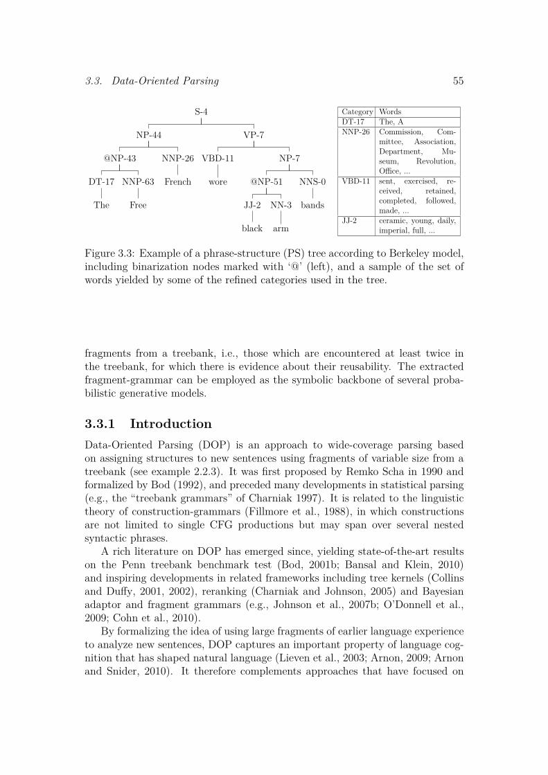
3.3. Data-Oriented Parsing 55
S-4
NP-44
@NP-43
DT-17
The
NNP-63
Free
NNP-26
French
VP-7
VBD-11
wore
NP-7
@NP-51
JJ-2
black
NN-3
arm
NNS-0
bands
Category WordsDT-17 The, ANNP-26 Commission, Com-
mittee, Association,Department, Mu-seum, Revolution,Office, ...
VBD-11 sent, exercised, re-ceived, retained,completed, followed,made, ...
JJ-2 ceramic, young, daily,imperial, full, ...
Figure 3.3: Example of a phrase-structure (PS) tree according to Berkeley model,including binarization nodes marked with ‘@’ (left), and a sample of the set ofwords yielded by some of the refined categories used in the tree.
fragments from a treebank, i.e., those which are encountered at least twice inthe treebank, for which there is evidence about their reusability. The extractedfragment-grammar can be employed as the symbolic backbone of several proba-bilistic generative models.
3.3.1 IntroductionData-Oriented Parsing (DOP) is an approach to wide-coverage parsing basedon assigning structures to new sentences using fragments of variable size from atreebank (see example 2.2.3). It was first proposed by Remko Scha in 1990 andformalized by Bod (1992), and preceded many developments in statistical parsing(e.g., the “treebank grammars” of Charniak 1997). It is related to the linguistictheory of construction-grammars (Fillmore et al., 1988), in which constructionsare not limited to single CFG productions but may span over several nestedsyntactic phrases.
A rich literature on DOP has emerged since, yielding state-of-the-art resultson the Penn treebank benchmark test (Bod, 2001b; Bansal and Klein, 2010)and inspiring developments in related frameworks including tree kernels (Collinsand Duffy, 2001, 2002), reranking (Charniak and Johnson, 2005) and Bayesianadaptor and fragment grammars (e.g., Johnson et al., 2007b; O’Donnell et al.,2009; Cohn et al., 2010).
By formalizing the idea of using large fragments of earlier language experienceto analyze new sentences, DOP captures an important property of language cog-nition that has shaped natural language (Lieven et al., 2003; Arnon, 2009; Arnonand Snider, 2010). It therefore complements approaches that have focused on
56 Chapter 3. Recycling Phrase-Structure Constructions
properties like lexicalization or incrementality, and might bring supplementarystrengths into other NLP tasks.
In this section we present a novel DOP model (Double-DOP) in which weextract a restricted yet representative subset of fragments: those recurring atleast twice in the treebank. The explicit representation of the fragments allowsus to derive simple ways of estimating probabilistic models on top of the symbolicgrammar. This and other implementation choices aim at making the methodologytransparent and easily replicable. The accuracy of Double-DOP is well within therange of state-of-the-art parsers currently used in other NLP-tasks, while offeringthe additional benefits of a simple generative probability model and an explicitrepresentation of grammatical constructions.
We present a number of technical contributions: (i) a way to restrict theset of fragments to only those that occur multiple times in the train set, (ii)a transform-backtransform approach that allows us to use off-the-shelf PCFGparsing techniques, and (iii) a way to integrate DOP with recent state-splittingapproaches (Petrov et al., 2006), yielding an even more accurate parser and abetter understanding of the relation between DOP and state-splitting.
In line with the symbolic/probabilistic separation conducted in the previouschapter we will first introduce the symbolic backbone of our DOP model (§3.4)and later on describe its stochastic instantiation (§3.6).
3.4 The symbolic backboneThe basic idea behind DOP is to allow arbitrarily large fragments from a treebankto be the elementary units of production of the grammar.
A fragment can be formally described as a subtree of a PS tree, where foreach node in the fragment either all or none of its child nodes are present in thesubtree. Fragments can be combined through the substitution operation to obtainthe PS tree of a new sentence. Figure 3.4 shows an example of how to obtain thecomplete syntactic tree in figure 3.1 by combining three elementary fragments.As in previous work, two fragments fi and fj can be combined (fi ○fj) only if theleftmost substitution site X↓ in fi has the same label as the root node of fj; inthis case the resulting tree will correspond to fi with fj replacing X. The DOPformalism is discussed in detail in e.g., Bod et al. (2003).
3.4.1 Explicit vs. Implicit GrammarsThe first step to build a DOP model is to define its symbolic grammar, i.e., the setof elementary fragments in the model. Early versions of DOP (e.g., Bod et al.,2003) aimed at extracting all subtrees of all trees in the treebank. The totalnumber of subtrees, however, is prohibitively large for non-trivial treebanks: itgrows exponentially with the length of the sentences, yielding the astronomically

3.4. The symbolic backbone 57
S
NP↓ VP
VBD
wore
NP↓○
NP
DT
The
NNP
Free
NNP
French
○
NP
JJ
black
NN
arm
NNS
bands
Figure 3.4: An example of a derivation of the syntactic structure in figure 3.1obtained combining three elementary fragments by means of the substitutionoperation ○. Substitution sites are marked with the symbol ↓.
large number of approximately 1046 for section 2-21 of the Penn WSJ treebank(see §3.5.2). DOP models that work with an explicit extraction of subtrees (Bod,1992, 2001b; Zuidema, 2007), thus resorted to random sampling or to specificheuristics to filter fragments based on their features (e.g., depth, number of lexicalor nonterminal elements in frontier). But, as we will show in section 3.5.2, themajority of the constructions extracted by most of these sampling techniquesoccur only once in the training corpus. For instance the chance that a randomlyextracted large fragment is reusable in a different structure is, for all practicalpurposes, 0. At the same time, any sampling technique will most likely fail toextract many relevant syntactic productions.
Goodman transformation Later DOP models have used the Goodman trans-formation (Goodman, 1996, 2003) to obtain a compact representation of all frag-ments in the treebank (Bod, 2003; Bansal and Klein, 2010). The transformationwas defined for some versions of DOP to an equivalent PCFG-based model, withthe number of rules extracted from each parse tree being linear in the size of thetrees.
This is possible by means of enriching the treebank with a unique index ifor every node N (becoming Ni) in the trees. Assuming that the treebank isbinarized, for every PCFG rule Aj → BkCl, 8 rules are extracted:
Aj → BC A → BCAj → BkC A → BkCAj → BCl A → BClAj → BkCl A → BkCl
Here we have reported only the symbolic part of the conversion. Goodmandefines also specific weights for each transformed rule, so that the model generates

58 Chapter 3. Recycling Phrase-Structure Constructions
subderivations with the same probabilities as various probabilistic DOP models.This transform, is used in most recent DOP parsers (e.g., Bod, 2003; Bansal andKlein, 2010). The grammar represents larger fragments only implicitly, by meansof the unique indices which function as locks, constraining every indexed node Ni
to the CFG production where it occurs in the training corpus.Bod has argued for the Goodman transform as the solution to the computa-
tional challenges of DOP (e.g., Bod, 2003); it is important to realize, however,that the resulting grammars are still very large: WSJ sections 2-21 yield about7.8 × 106 rules in the basic version of Goodman’s transform.2 Moreover, thetransformed grammars differ from untransformed DOP grammars in that largerfragments are no longer explicitly represented. Rather, information about theirfrequency is distributed over many CFG-rules: if a construction occurs n timesand contains m context-free productions, Goodman’s transform uses the weightsof 7nm +m rules to encode this fact. Thus, the information that the idiomaticfragment (PP (IN “out”) (PP (IN “of”) (NP (NN “town”))))) occurs 3 times inWSJ sections 2-21, is distributed over 132 rules. This way, an attractive featureof DOP, viz. the explicit representation of the ‘productive units’ of language, islost.3
3.5 Finding Recurring FragmentsIn the current work we return to the first approach, and explicitly extract asubset of fragments from the training treebank. We believe that an explicitrepresentation of fragments in a grammar could provide great advantages forbetter understanding the model, since it allows us to reproduce the process bywhich syntactic pieces are combined to form sentential structures. Moreoverin several applications it is conceptually easier to deal with explicit grammarproductions, as for instance in machine translation systems which need to resolvea mapping between syntactic productions of two distinct languages.
Unfortunately, as explained above, explicit fragment grammars can grow ex-tremely large in size. To limit the fragment set size, we use a simple but heretoforeunexplored constraint: we extract only those fragments that occur two or moretimes in the treebank. This intuition follows the natural assumption, commonin many current linguistic theories, to consider a construction linguistically rele-vant if there is empirical evidence about its reusability in a representative corpus.Thus with Double-DOP we hope to overcome some of the limitations of pre-vious probabilistic extensions of CFGs as well as the problem of efficiency and
2About 106 lexical and 6.8 × 10⁶ internal rules. This has been calculated from the treebankwhich was binarized as in our experiments.
3Bansal and Klein (2010) address this issue for contiguous constructions by extending theGoodman transform with a ‘Packed Graph Encoding’ for fragments that “bottom out in termi-nals”. However, constructions with variable slots, such as whether S or not, are left unchanged.
3.5. Finding Recurring Fragments 59
reproducibility of previous DOP models based on the extraction of an explicitfragment-grammars.
The idea of working with fragments occurring two or more times in the tree-bank, can be seen as related to the held-out estimation procedure used in DOP*(Zollmann and Sima’an, 2005). In this work, fragments are extracted from asubset of the training treebank (the extraction corpus, EC) and their weights areestimated on the remaining part (the held-out corpus, HC) in order to maximizeits likelihood. As a result, the fragments which obtain non-zero weights in thefinal grammar are those occurring both in EC and HC. If HC consists of a singletree (leave-one-out), and by repeating the procedure such that each tree in thetraining corpus is used once as the held-out data (K-fold cross-validation), thefinal grammar will contain exactly those fragments occurring at least twice in thetraining corpus.
In the remaining of this section we describe the algorithm for extracting theset of recurring fragments from a treebank, which will constitute our symbolicgrammar, and illustrate some properties of the selected constructions. In §3.6 and§3.7 we will propose a number of probabilistic instantiations of the underlyingsymbolic model.
3.5.1 The search algorithmExtracting recurring fragments in a large treebank is not a trivial task: a naiveapproach that filters a complete table of fragments together with their frequencieswould fail because that set, in a reasonably sized treebank, is astronomically large.Instead, we use an efficient kernel-based algorithm, which is conceptually similarto previously proposed methods using this technique (Collins and Duffy, 2001,2002; Moschitti, 2006). The main difference, however, is that, while in previousstudies kernels are mainly used to numerically quantify the similarity between twotrees, in the current work we are interested in identifying the actual constructionsthey share, i.e., the common largest (or maximal) fragments.
Our search algorithm4 iterates over every pair of trees in the treebank andlooks for common maximal fragments. More precisely we extract only the largestshared fragments for all pairs of trees in the treebank. All subtrees of these ex-tracted fragments necessarily also occur at least twice, but they are only explicitlyrepresented in our extracted set if they happen to form a largest shared fragmentfrom another pair of trees. Hence, if a large tree occurs twice in the treebank thealgorithm will extract from this pair only the full tree as a fragment and not allits (exponentially many) subtrees.
Figure 3.5 shows an example of a pair of trees ⟨α,β⟩ being compared. All thenon-terminal nodes of the two trees are indexed following a depth-first ordering
4The implemented software for extracting recurring fragments (FragmentSeeker) is availableat http://staff.science.uva.nl/˜fsangati/.

60 Chapter 3. Recycling Phrase-Structure Constructions
(as in figure 2.9). The algorithm builds a chart M with one column for everyindexed non-terminal node αi in α, and one row for every indexed non-terminalnode βj in β. Each cell M⟨i, j⟩ identifies a set of indices corresponding to thelargest fragment in common between the two trees starting from αi and βj. Thisset is empty if αi and βj differ in their labels, or they do not have the same listof child nodes. Otherwise (if both the labels and the lists of children match) theset is computed recursively as follows:
M⟨i, j⟩ = {αi} ⋃⎛⎝ ⋃c={1,2,...,∣ch(α)∣}
M⟨ch(αi, c), ch(βj, c)⟩⎞⎠
(3.1)
where ch(α) returns the indices of α’s children, and ch(α, c) the index of itscth child. The procedure to recursively compute the maximal shared fragmentsbetween two nodes (Ni,Nj) of a pair of PS trees is described in the algorithm infigure 3.5.
After filling the chart, the algorithm extracts the set of recurring fragments,and stores them in a table to keep track of their counts. This is done by convertingback each fragment implicitly defined in every cell-set,5 and filtering out thosethat are properly contained in others.6
The time complexity of the overall procedure, is O(n2 ⋅m2) where n is the sizeof the treebank and m the number of nodes in the biggest tree of the corpus.7 Interms of space the number of maximal fragments which are extracted for everypair of trees is in the worst case m2.
3.5.2 A case study on the Penn WSJIn this section we describe some statistics derived from testing our extractionprocedure on the Penn WSJ corpus Marcus et al. (1993). We have restricted thetreebank to the 39,832 structures of sections 2-21 after removing null productionsand traces. Differently from the preprocessing in later experiments the treebankhere is not binarized and functional tags (SBJ, TMP, etc...) are kept.
Figure 3.6 reports some statistics on the set of all maximal fragments whichare extracted from the treebank. The total number of extracted fragments types
5A cell-set containing a single index corresponds to the fragment including the node withthat index together with all its children.
6In a second pass over the treebank, exact counts can be obtained for each fragment inthe extracted set. However, the approximate counts returned by the extraction algorithm areextremely close to the exact values.
7In terms of empirical computation time, using a 2.5 GHz processor machine, our programtakes about around 50-CPU hours for WSJ (sections 2-21). Although our code could still beoptimized further, it does already allow for running the job on N CPUs in parallel, reducingthe time required by a factor N (less than 3 hours with 16-CPUs). Computing time of coursebecomes problematic for very large treebanks, but we are optimistic about the effectiveness ofapproximate strategies when training sets becomes very large.

3.5. Finding Recurring Fragments 61
S
NP
PRP
I
VP
VBP
say
SBAR
S
NP
PRP
they
VP
VBP
are
ADJP
JJ
ready
.
.
S
NP
NNS
Analysts
VP
VBP
say
SBAR
S
NP
NNP
USAir
VP
VBZ
has
NP
JJ
great
NN
promise
.
.
S NP
PRP
VP
VB
PSB
AR
S NP
PRP
VP
VB
PA
DJP
JJ .
S × ×NP × ×
NNSVP × ×
VBP × ×SBAR ×
S × ×NP × ×
NNPVP ×
VBZNP
JJ ×NN
. ×α β
Figure 2: Left: example of two trees sharing a single maximum fragment, circled in the two trees. Right: the chartM which is used in the dynamic algorithm to extract all maximum fragments shared between the two trees. Thehighlighted cells in the chart are the ones which contribute to extract the shared fragment. The marked cells are thosefor which the corresponding nodes in the two tree have equivalent labels but differ in their lists of child nodes.
the treebank to look for common fragments. Fig-ure 2 shows an example of a pair of trees �α,β� be-ing compared. The algorithm builds a chart M withone column for every indexed non-terminal node αi
in α, and one row for every indexed non-terminalnode βj in β. Each cell M�i, j� identifies a set of in-dices corresponding to the largest fragment in com-mon between the two trees starting from αi and βj .This set is empty if αi and βj differ in their labels,or they don’t have the same list of child nodes. Oth-erwise (if both the labels and the lists of childrenmatch) the set is computed recursively as follows:
M�i, j� = {αi} ∪ �
c={1,2,...,|ch(α)|}M�ch(αi, c), ch(βj , c)�
(1)
where ch(α) returns the indices of α’s children, andch(α, c) the index of its cth child.
After filling the chart, the algorithm extracts theset of recurring fragments, and stores them in a ta-ble to keep track of their counts. This is done byconverting back each fragment implicitly defined inevery cell-set2, and filtering out those that are prop-erly contained in others.
In a second pass over the treebank, exact countsare obtained for each fragment in the extracted set.
2A cell-set containing a single index corresponds to the frag-ment including the node with that index together with all itschildren.
Parse trees in the training corpus are not necessarilycovered entirely by recurring fragments; to ensurecoverage, we also include in the symbolic backboneof our Double-DOP model all PCFG-productionsnot included in the set of extracted fragments.
2.2 Comparison with previous DOP work
Explicit grammars The number of recurring frag-ments in our symbolic grammar, extracted fromthe training sections of the Penn WSJ treebank3, isaround 1 million, and thus is significantly lower thanprevious work extracting explicit fragments (e.g.,Bod, 2001, used more than 5 million fragments upto depth 14).
When looking at the extracted fragments we askif we could have predicted which fragments occurtwice or more. Figure 3 attempts to tackle this ques-tion by reporting some statistics on the extractedfragments. The majority of fragments are rathersmall with a limited number of words or substitutionsites in the frontier. Yet, there is a significant por-tion of fragments, in the tail of the distribution, withmore than 10 words or substitution sites. Since thespace of all fragments with such characteristics isenormously large, selecting big recurring fragmentsusing random sampling technique is like finding aneedle in a haystack. Hence, random sampling pro-cesses (like Bod, 2001), will tend to represent fre-
3This is after the treebank has been preprocessed. See alsosection 4.
S
NP
PRP
I
VP
VBP
say
SBAR
S
NP
PRP
they
VP
VBP
are
ADJP
JJ
ready
.
.
S
NP
NNS
Analysts
VP
VBP
say
SBAR
S
NP
NNP
USAir
VP
VBZ
has
NP
JJ
great
NN
promise
.
.
S NP
PRP
VP
VB
PSB
AR
S NP
PRP
VP
VB
PA
DJP
JJ .
S × ×NP × ×
NNSVP × ×
VBP × ×SBAR ×
S × ×NP × ×
NNPVP ×
VBZNPJJ ×
NN. ×α β
Figure 2: Left: example of two trees sharing a single maximum fragment, circled in the two trees. Right: the chartM which is used in the dynamic algorithm to extract all maximum fragments shared between the two trees. Thehighlighted cells in the chart are the ones which contribute to extract the shared fragment. The marked cells are thosefor which the corresponding nodes in the two tree have equivalent labels but differ in their lists of child nodes.
the treebank to look for common fragments. Fig-ure 2 shows an example of a pair of trees �α,β� be-ing compared. The algorithm builds a chart M withone column for every indexed non-terminal node αi
in α, and one row for every indexed non-terminalnode βj in β. Each cell M�i, j� identifies a set of in-dices corresponding to the largest fragment in com-mon between the two trees starting from αi and βj .This set is empty if αi and βj differ in their labels,or they don’t have the same list of child nodes. Oth-erwise (if both the labels and the lists of childrenmatch) the set is computed recursively as follows:
M�i, j� = {αi} ∪ �
c={1,2,...,|ch(α)|}M�ch(αi, c), ch(βj , c)�
(1)
where ch(α) returns the indices of α’s children, andch(α, c) the index of its cth child.
After filling the chart, the algorithm extracts theset of recurring fragments, and stores them in a ta-ble to keep track of their counts. This is done byconverting back each fragment implicitly defined inevery cell-set2, and filtering out those that are prop-erly contained in others.
In a second pass over the treebank, exact countsare obtained for each fragment in the extracted set.
2A cell-set containing a single index corresponds to the frag-ment including the node with that index together with all itschildren.
Parse trees in the training corpus are not necessarilycovered entirely by recurring fragments; to ensurecoverage, we also include in the symbolic backboneof our Double-DOP model all PCFG-productionsnot included in the set of extracted fragments.
2.2 Comparison with previous DOP work
Explicit grammars The number of recurring frag-ments in our symbolic grammar, extracted fromthe training sections of the Penn WSJ treebank3, isaround 1 million, and thus is significantly lower thanprevious work extracting explicit fragments (e.g.,Bod, 2001, used more than 5 million fragments upto depth 14).
When looking at the extracted fragments we askif we could have predicted which fragments occurtwice or more. Figure 3 attempts to tackle this ques-tion by reporting some statistics on the extractedfragments. The majority of fragments are rathersmall with a limited number of words or substitutionsites in the frontier. Yet, there is a significant por-tion of fragments, in the tail of the distribution, withmore than 10 words or substitution sites. Since thespace of all fragments with such characteristics isenormously large, selecting big recurring fragmentsusing random sampling technique is like finding aneedle in a haystack. Hence, random sampling pro-cesses (like Bod, 2001), will tend to represent fre-
3This is after the treebank has been preprocessed. See alsosection 4.
α β
S NP
PRP
VP
VBP
SBA
RS NP
PRP
VP
VBP
AD
JP JJ .
S × ×NP × ×
NNSVP × ×
VBP × ×SBAR ×
S × ×NP × ×
NNPVP ×
VBZNPJJ ×
NN. ×
Algorithm: ExtractMaxFragment(Ni,Nj)Input: two PS nodes (Ni,Nj)Output: a set of nodes representing the largest
fragment rooted in Ni and Nj
beginif Ni ≠ Nj then return {};NodeSet← {Ni};if Ni.daughters = Nj.daughters thenfor d ∈ (1,2, . . . ,Ni.daughters.size) doDi ← Ni[d];Dj ← Nj[d];NodeSetD ←ExtractMaxFragment(Di,Dj);NodeSet.union(NodeSetD);
return NodeSet;
Figure 3.5: Above: example of two trees sharing a single maximum fragment,highlighted in the two trees. Below: the chart used in the algorithm to extractall maximum fragments shared between the two trees, and the pseudocode ofthe algorithm used for extracting the largest fragment rooted in two nodes oftwo PS trees. In the chart, the highlighted cells are the ones which contributeto extracting the shared fragment. The cells marked with a cross are those forwhich the corresponding nodes in the two tree have equivalent labels.

62 Chapter 3. Recycling Phrase-Structure Constructions
is 527,217, and their distribution with respect to their depths, reported on thegraph of the same figure, shows that fragments of depth 3 and 4 are the mostabundant recurring fragments in the corpus. Their frequency distribution followsZipf’s law as shown in figure 3.7.
Figure 3.8 shows the distribution of the total number of fragments tokenswhich are present in the same treebank, with respect to their depths and max-imum branching. The maximum branching of a fragment corresponds to themaximum number of daughters of the most prolific node. From the figure wecan see that this variable is the primary factor to affect the number of subtreespresent in a tree structure. The total number of fragments without any restrictionin depth and branching, is estimated to be 8.7 ⋅ 1046.8 It follows that the portionof fragment tokens which are recurring in the treebank (the shaded area in thegraph) is an extremely small fraction9 of all possible fragments.
When looking at the extracted fragments we ask if we could have predictedwhich fragments occur twice or more. Figure 3.10 attempts to tackle this questionby reporting some statistics on the extracted fragments. In particular it shows thedistribution of the recurrent fragments types according to several features: depth,number of words, and number of substitution sites. Not surprisingly most of thefrequent recurring fragments have low values for these features: the majority offragments are rather small with a limited number of words or substitution sitesin the frontier. Nevertheless there is still a significant portion of fragments, in thetail of the distribution, with more than 10 words (or substitution sites). Sincethe space of all fragments with such characteristics is enormously large, selectingbig recurring fragments using random sampling technique is like finding a needlein a haystack. Hence, random sampling processes (like Bod, 2001b), will tendto represent frequent recurring constructions such as from NP to NP or whetherS or not, together with infrequent overspecialized fragments like from Houstonto NP, while missing large generic constructions such as everything you alwayswanted to know about NP but were afraid to ask. These large constructions areexcluded completely by models that only allow elementary trees up to a certaindepth (typically 4 or 5) into the symbolic grammar (Zollmann and Sima’an, 2005;Zuidema, 2007; Borensztajn et al., 2009), or only elementary trees with exactlyone lexical anchor (Sangati and Zuidema, 2009).
Finally, in figure 3.9 we have reported the most frequently recurring fragmentsin the WSJ containing the verb “say” (when it is a present tense verb). This kindof statistics, can give an insight on the specific template constructions of thisparticular verb.
8This number is calculated by summing the number of subtrees ω(Ni) rooted in every nodeNi of every tree in the treebank. ω(Ni) is calculated recursively: ω(Ni) =∏D∈d(Ni) (ω(D) + 1),where d(Ni) returns the list of daughter nodes of Ni. If N is a terminal node ω(N) = 0.
9In the graph, the shaded area representing this tiny fraction (7.1 ⋅ 10−41), is visible becauseof the logarithmic scale in the y-axes.

3.5. Finding Recurring Fragments 63
Depth Types Tokens1 27,893 1,570,8692 86,512 1,549,5233 138,709 1,428,7774 128,927 923,3155 83,218 455,4486 40,524 179,5487 14,849 52,4248 4,677 14,1339 1,343 3,69210 398 95111 96 21312 39 9513 14 2814 6 1615 4 816 3 817 2 518 2 420 1 2
Total 527,217 6,179,059
0
250,000
500,000
750,000
1,000,000
1,250,000
1,500,000
1,750,000
2,000,000
0
20,000
40,000
60,000
80,000
100,000
120,000
140,000
160,000
1 2 3 4 5 6 7 8 9
Num
ber of Token
s
Num
ber of Types
Depth
Types
Tokens
Figure 3.6: Distribution of the types and tokens frequencies of the recurringmaximal fragment with respect to their depths. Fragments are extracted fromsections 2-21 of the Penn WSJ Treebank.
Figure 3.7: Zipf distribution of the recurring fragments extracted from section02-21 of the Penn WSJ Treebank.

64 Chapter 3. Recycling Phrase-Structure Constructions
0 5
10
15
20
25
30
35
40
45
50
0 1
2 3
4 5
6 7
8 9
10 11
12 13
14 15
16 17
18 19
20 21
22 23
24 25
26 27
28 29
30 31
32 33
34 35
36
LOG10 FREQUENCY (TOKENS)
DEPTH
1
2 (binary branching)
3
4
5 6
7
8
9-‐11 13-‐15
16-‐50
51 R1 R2
12
R3
Figure3.8:D
istributionofthe
totalnumberoffragm
entstokenswhich
arepresentin
thetreesofsections2-21
ofthePenn
WSJ
Treebank,with
respectto
thefragm
entdepths
(horizontalaxes,with
depth=1
standingfor
singletree
nodes,anddepth=
2forC
FG-rules).Every
linecorrespondsto
thetotalnum
beroffragmentsatdifferentdepth
values,when
limiting
them
aximum
branchingofthe
fragments
toa
certainconstant
(thenum
berreported
closeto
theline).
The
maxim
umbranching
ofafragm
entis
definedto
bethe
maxim
umnum
berofdaughters
inthe
most
prolificnode
ofthefragm
ent.T
heshaded
areaat
thebottom
ofthe
graphrepresents
theportion
ofrecurring
fragments
which
weextract
fromthe
treebank(the
maxim
alfragmentsshared
betweenatleasttwo
trees).R1
isthesub-portion
includingfragm
entswith
onlyunary
branching(alm
ostallarerecurring
fragments),and
similarly
R2
andR
3representsub-portionsw
ithfragm
entswith
maxim
umbranching
2and
3.

3.5. Finding Recurring Fragments 65
VBP
“say”
VP
VBP
“say”
SBAR
VP
VBP
“say”
SBAR
S
VP
VBP
“say”
SBAR
S
NP-SBJ VP
525 342 293 249
S
NP-SBJ VP
VBP
“say”
SBAR
.
“.”
VP
VBP
“say”
S
NP-SBJ VP
VBP
“say”
SBAR
S
.
“.”
S
NP-SBJ VP
VBP
“say”
SBAR
S
NP-SBJ VP
.
“.”
173 157 140 120
S
S-TPC ,
“,”
NP-SBJ VP
VBP
“say”
.
“.”
VP
VBP
“say”
SBAR
S
NP-SBJ
PRP
VP
S
NP-SBJ VP
VBP
“say”
VP
VBP
“say”
SBAR
S
NP-SBJ VP
MD VP
74 73 55 47
PRN
,
“,”
S
NP-SBJ VP
VBP
“say”
,
“,”
VP
VBP
“say”
SBAR
S
NP-SBJ
PRP
“they”
VP
S
NP-SBJ VP
VBP
“say”
SBAR
VP
VBP
“say”
SBAR
IN
“that”
S
47 46 46 45
Figure 3.9: The most frequent fragments containing the verb say, when it is apresent tense verb (VBP). Below each fragment we report the exact frequencywith which it occurs in the WSJ sec 02-21. For example, the second fragmentat the top of the figure (occurring 342 times) illustrates a specific template con-struction of the verb, which requires a relative or subordinate clause (SBAR) asfirst and only argument to its right; this specific construction accounts for 65%of the occurrences of “say”.

66 Chapter 3. Recycling Phrase-Structure Constructions
100
101
102
103
104
105
106
0 10 20 30 40 50 60
Num
ber
of F
ragm
ents
(ty
pes)
Depth / Words / Substitution Sites
DepthWords
Substitution Sites
Figure 3.10: Distribution of the recurring fragments types according to severalfeatures: depth, number of words, and number of substitution sites. Their corre-sponding curves peak at 3 (depth), 1 (words), and 3 (substitution sites).
3.6 The probability modelThe set of recurring fragments can be used as the symbolic backbone of a prob-abilistic parser. Like CFGs, our symbolic model produces extremely many parsetrees for a given test sentence.10 We therefore need to disambiguate betweenthe possible parses by means of a probability model that assigns probabilities tofragments, and defines a proper distribution over the set of possible full parsetrees.
For every nonterminal X in our grammar we want to have (see also equa-tion 2.6):
∑f∈FX
p(f) = 1 (3.2)
where FX is the set of fragments in our symbolic grammar rooted in X. Addingprobabilities turns our grammars into probabilistic tree substitution grammars(PTSGs).
10In particular our Double-DOP grammar extracted from a treebank has the same stronggenerative power of the subsuming CFG: it generate the same tree structures of the CFGextracted from the same treebank.
3.6. The probability model 67
A derivation d = f1, f2, . . . , fn of T is a sequence of fragments that throughleft-most substitution produces T . The probability of a derivation is computedas the product of the probabilities of each of its fragments.
P (d) =∏f∈dp(f) (3.3)
In §3.6.2 we describe ways of obtaining different probability distributions overthe fragments in our grammar, but we first illustrate how to use standard PCFGparsing techniques given a probabilistic model.
3.6.1 ParsingIt is possible to define a simple transform of our probabilistic fragment grammar,such that off-the-shelf parsers can be used. In order to perform the PTSG/PCFGconversion, every fragment in our grammar must be mapped to a CFG rule whichwill keep the same probability as the original fragment. The corresponding rulewill have as the left hand side the root of the fragment and as the right hand sideits yield, i.e., a sequence of terminals and non-terminals (substitution sites).
It might occur that several fragments are mapped to the same CFG rule.11
These are interesting cases of syntactic ambiguity as shown in figure 3.11. Inorder to resolve this problem we need to map each ambiguous fragment to twounique CFG rules chained by a unique artificial node, as shown at the bottomof the same figure. To the first CFG rule in the chain we assign the probabilityof the fragment, while the second will receive probability 1, so the product givesback the original probability. The ambiguous and unambiguous PTSG/PCFGmappings need to be stored in a table, in order to convert back the compressedCFG derivations to the original PTSG model after parsing.
Such a transformed PCFG will generate the same derivations as the originalPTSG grammar with identical probabilities. The resulting grammar is more eco-nomic than previously proposed transformations: it needs only one PCFG rulesper elementary tree, and two for the ambiguous fragment. Previous approaches(e.g., Zuidema, 2007, and others) use a separate rule for each CFG-productioninside an elementary tree.
In our experiment we use a standard PCFG parser to produce a list of k-bestViterbi derivations. These, in turn, will be used to maximize possible objectivesas described in section 3.6.3.
11In our binarized treebank we have 31,465 fragments types that are ambiguous in this sense(about 6% of the total number of extracted fragments). On average 2.05 ambiguous fragmentsmap to the same CFG rule.
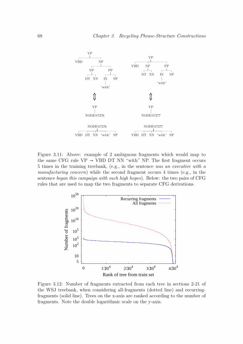
68 Chapter 3. Recycling Phrase-Structure Constructions
VP
VBD NP
NP
DT NN
PP
IN
“with”
NP
VP
VBD NP
DT NN
PP
IN
“with”
NP
⇕ ⇕VP
NODE@7276
VP
NODE@7277
NODE@7276
VBD DT NN “with” NP
NODE@7277
VBD DT NN “with” NP
Figure 3.11: Above: example of 2 ambiguous fragments which would map tothe same CFG rule VP → VBD DT NN “with” NP. The first fragment occurs5 times in the training treebank, (e.g., in the sentence was an executive with amanufacturing concern) while the second fragment occurs 4 times (e.g., in thesentence began this campaign with such high hopes). Below: the two pairs of CFGrules that are used to map the two fragments to separate CFG derivations.
510
102103
105
1010
1020
1050
0 1⋅104 2⋅104 3⋅104 4⋅104
Num
ber
of f
ragm
ents
Rank of tree from train set
Recurring fragmentsAll fragments
Figure 3.12: Number of fragments extracted from each tree in sections 2-21 ofthe WSJ treebank, when considering all-fragments (dotted line) and recurring-fragments (solid line). Trees on the x-axis are ranked according to the number offragments. Note the double logarithmic scale on the y-axis.

3.6. The probability model 69
3.6.2 Inducing probability distributionsRelative Frequency Estimate (RFE) The simplest way to assign probabil-ities to fragments is to make them proportional to their counts12 in the trainingset. When enforcing equation 3.2, that gives the Relative Frequency Estimate(RFE):
pRFE(f) =count(f)
∑f ′∈Froot(f) count(f ′)(3.4)
Unlike RFE for PCFGs, however, the RFE for PTSGs has no clear probabilis-tic interpretation. In particular, it does not yield the maximum likelihood solu-tion, and when used as an estimate for an all-fragments grammar, it is stronglybiased since it assigns the great majority of the probability mass to big frag-ments (Bonnema et al., 1999): grammars that implicitly encode all fragmentsfound in a treebank are strongly biased to over-represent big fragments found inthe largest constructions in the treebank.13 DOP models relying on Goodman’stransform, need therefore to counteract this tendency. Bansal and Klein (2010),for instance, rely on a sophisticated tuning technique to correctly adjust theweights of the rules in the grammar. In our Double-DOP approach, instead, thisbias is much weaker as the number of fragments extracted from each tree variesmuch less (it ranges between 4 and 1,759) as shown in figure 3.12. Although thisdoes not solve all theoretical issues, it makes RFE a reasonable choice.
Equal Weights Estimate (EWE) Various other ways of choosing the weightsof a DOP grammar have been worked out. The best empirical results have beenreported by Bod (2003) with the EWE proposed by Goodman (2003). Goodmandefined it for grammars in the Goodman transform, but for explicit grammars itbecomes:
wEWE(f) = ∑T ∈T
count(f, T )∣{f ′ ∈ T}∣ (3.5)
pEWE(f) = wEWE(f)∑f ′∈Froot(f) wEWE(f ′)
(3.6)
where the first sum is over all parse trees T in the treebank (T ), count(f, T )gives the number of times fragment f occurs in T , and ∣{f ′ ∈ T}∣ is the totalnumber of subtrees of T that were included in the symbolic grammar.
Maximum Likelihood Estimate (MLE) As an alternative estimate, we alsotry to find the probability distribution which maximizes the likelihood of the
12We refer to the counts of each fragment as returned by our extraction procedure describedin §3.5.1.
13In fact, the number of extracted fragments increase exponentially with the size of the tree,and the great majority of the entire set of fragments belongs to the largest tree in the treebank

70 Chapter 3. Recycling Phrase-Structure Constructions
training treebank. For this we apply the Inside-Outside algorithm (Lari andYoung, 1990), an instance of the Expectation-Maximization algorithm (EM, seealso Prescher, 2003). The original version of IO is defined over string rewritingPCFGs, and maximizes the likelihood of the training set consisting of plain sen-tences. Reestimation shifts probability mass between alternative parse trees fora sentence. In contrast, our grammars consist of fragments of various sizes, andour training set of parse trees. Reestimation here shifts probability mass betweenalternative derivations for a parse tree (see also section 2.3.3).
In our EM experiments, we utilize a special-purpose implementation of IO forTSG as illustrate in algorithm 1 (p. 72). We start from an initial probabilitydistribution14 p0 over the fragments in F . The expectation step is done in stepA and B, which compute the inside and outside probabilities respectively. Morespecifically, for each parse tree T in the treebank, there are 3 different quantitiesthat we keep track of in the algorithm, which are also illustrated in figure 3.13:
• InsideNode(n): the inside probability of node n in T . It is computed asthe sum of all the sub-derivations generating the subtree of T starting fromn and ending in the lexical nodes under n.
• InsideFrag(f, n): the inside probability of all sub-derivations starting withfragment fn and generating the same subtree starting from n and ending inthe lexical nodes under n (as above).
• OutsideNode(n): the outside probability of node n in T . It is computed asthe sum of all the derivations generating the subtree of T starting on theroot node, and including in its yield n as the only substitution site, and alllexical nodes outside n.
In step C of algorithm 1 the maximization step is performed, reestimating theprobabilities of the fragments. The algorithm is guaranteed to produce a sequenceof reestimated probabilities p1, p2, . . . , pn for which the likelihood of the trainingcorpus monotonically increases (see also equation 2.22).
3.6.3 Maximizing ObjectivesMPD The easiest objective in parsing, is to select the most probable derivation(MPD), obtained by maximizing equation 3.3. This can be done efficiently bycomputing the best Viterbi derivation.
14In our EM experiments we used the RFE from section 3.6 to obtain the initial probabilitydistribution for the IO algorithm.

3.6. The probability model 71
S
A
D
d
E
e
B
F
f
G
g
C
H
h
I
i
Outside(B)
Inside(B)
Figure 3.13: Illustration of the inside and outside probabilities of node B in aparse tree, as defined in algorithm 1. The contribution of the dashed fragment fto the inside probability is defined as InsideFrag(f).
MPP A DOP grammar can often generate the same parse tree T through dif-ferent derivations D(T ) = d1, d2, . . . dm. The probability of T is therefore obtainedby summing the probabilities of all its possible derivations.
P (T ) = ∑d∈D(T )
p(d) = ∑d∈D(T )
∏f∈dp(f) (3.7)
An intuitive objective for a parser is to select, for a given sentence, the parsetree with highest probability according to equation 3.7, i.e., the most prob-able parse (MPP): unfortunately, identifying the MPP is computationally in-tractable (Sima’an, 1996). However, we can approximate the MPP by deriving alist of k-best derivations, summing up the probabilities of those resulting in thesame parse tree, and select the tree with maximum probability.
MCP, MRS Following Goodman (1998), Sima’an (1999, 2003), and others, wealso consider other objectives, in particular, the max constituent parse (MCP),and the max rule sum (MRS), which are all instances of the minimum Bayes riskdecoding (see Smith 2011, p. 163).
MCP maximizes a weighted average of the expected labeled recall L/NC and(approximated) labeled precision L/NG under the given posterior distribution,where L is the number of correctly labeled constituents, NC the number of con-stituents in the correct tree, and NG the number of constituents in the guessed

72 Chapter 3. Recycling Phrase-Structure Constructions
Algorithm: IOTSG(T , F, p0, ε)Input: T :treebank; F : fragments; p0: initial prob. distr. over F ; ε: stop thresholdOutput: p = {p1, p2, . . . , pn} : reestimated probabilities over FbeginPreviousLikelihood←Ð 0;CurrentLikelihood←Ð 1;iter ←Ð 0;while true dofor fragment f ∈ F do count(f)←Ð 0;for parsetree T ∈ T dofor node n ∈ t do{OutsideNode(n), InsideNode(n)}←Ð 0;for fragment f ∈ F , f ∈ T , f rooted in n doInsideFragment(f, n)←Ð 0;
// A) Compute Inside Probabilitiesfor non-lexical node n ∈ T (bottom-up) dofor fragment f ∈ F , f ∈ T , f rooted in n doInsideFrag(f, n)←Ð piter(f);for node s ∈ subSites(f, T ) doInsideFrag(f, n)∗ = InsideNode(s);InsideNode(n)+ = InsideFrag(f, n);
// B) Compute Outside ProbabilitiesOutsideNode(root(T ))←Ð 1;for non-lexical node n ∈ T (top-down) dofor fragment f ∈ F , f ∈ T , f rooted in n dofor node s ∈ subSites(f, T ) do
OutsideNode(s)+ = OutsideNode(n) ∗ InsideFrag(f, n)InsideNode(s) ;
// C) Reestimate Fragments ProbabilitiesProbTree←Ð InsideNode(root(T ));for non-lexical node n ∈ T dofor fragment f ∈ F , f ∈ T , f rooted in n do
count(f)+ = OutsideNode(n) ∗ InsideFrag(f, n)ProbTree
;
CurrentLikelihood∗ = ProbTree;
for fragment f ∈ F do piter+1(f)←Ðcount(f)
∑f ′∈F, root(f ′)=root(f) count(f ′);
if CurrentLikelihood − PreviousLikelihood < ε then return p ;PreviousLikelihood←Ð CurrentLikelihood;iter ←Ð iter + 1;
Algorithm 1: Pseudocode for the Inside-Outside algorithm reestimating the probabilitydistributions of the TSG fragments, in order to maximize the probability of the trainingtreebank.

3.7. Implementation 73
tree.15 Recall is easy to maximize since the estimated NC is constant. L/NC canbe in fact maximized in:
T = arg maxT
∑lc∈T
P (lc) (3.8)
where lc ranges over all labeled constituents in T and P (lc) is the marginalizedprobability of all the derivation trees in the grammar yielding the sentence underconsideration which contains lc.
Precision, instead, is harder because the denominator NG depends on thechosen guessed tree. Goodman (1998) proposes to look at another metric whichis strongly correlated with precision, which is the mistake rate (NG − L)/NC
that we want to minimize. We combine recall with mistake rate through linearinterpolation:
T = arg maxT
E( LNC
− λNG −LNC
) (3.9)
= arg maxT
∑lc∈T
P (lc) − λ(1 − P (lc)) (3.10)
where 3.10 is obtained from 3.9 assuming NC constant, and the optimal level forλ has to be evaluated empirically.
Unlike MPP, the MCP can be calculated efficiently using dynamic program-ming techniques over the parse forest. However, in line with the aims of thischapter to produce an easily reproducible implementation of DOP, we developedan accurate approximation of the MCP using a list of k-best derivations, such asthose that can be obtained with an off-the-shelf PCFG parser.
We do so by building a standard CYK chart, where every cell correspondsto a specific span in the test sentence. We store in each cell the approximatedprobability of seeing every label in the grammar yielding the corresponding span,by marginalizing the probabilities of all the parse trees in the obtained k-bestderivations that contains that label covering the same span. We then computethe Viterbi-best parse maximizing equation 3.10.
We implement max rule sum (MRS) in a similar way, but do not only keeptrack of labels in every cell, but of each CFG rule that span the specific yield (seealso Sima’an, 1999, 2003). We have not implemented the max rule product (MRP)where marginal posterior probabilities are multiplied instead of added (Petrov andKlein, 2007; Bansal and Klein, 2010).
3.7 ImplementationIn order to build and test our Double-DOP model, we employ the Penn WSJTreebank (Marcus et al., 1993), and other treebanks of various languages (see
15For a definition of recall and precision see also §3.9.
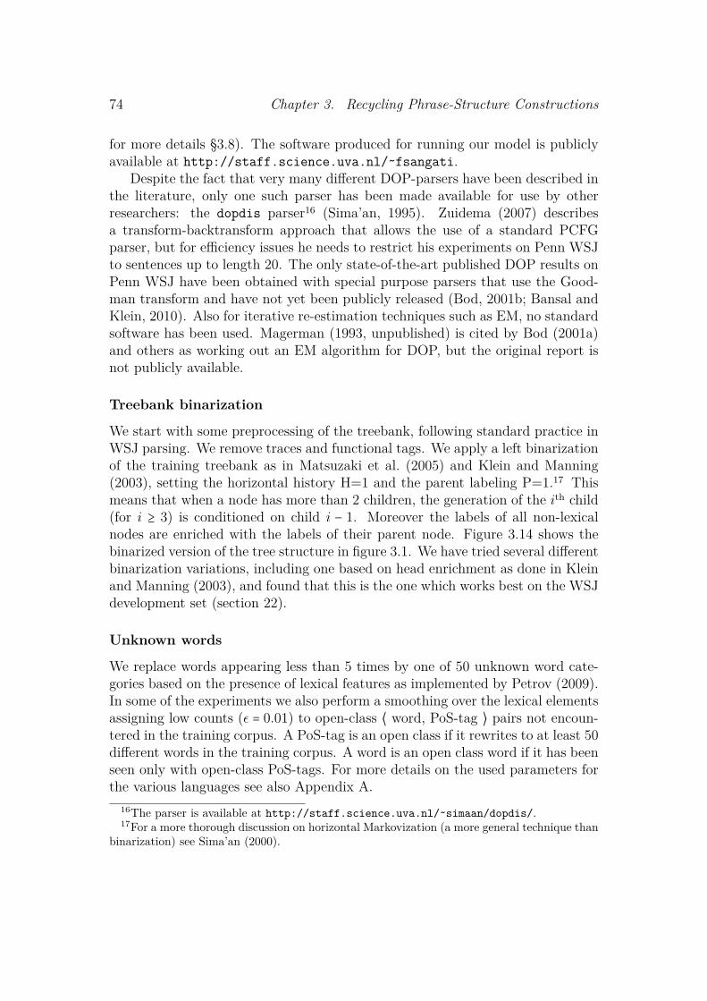
74 Chapter 3. Recycling Phrase-Structure Constructions
for more details §3.8). The software produced for running our model is publiclyavailable at http://staff.science.uva.nl/˜fsangati.
Despite the fact that very many different DOP-parsers have been described inthe literature, only one such parser has been made available for use by otherresearchers: the dopdis parser16 (Sima’an, 1995). Zuidema (2007) describesa transform-backtransform approach that allows the use of a standard PCFGparser, but for efficiency issues he needs to restrict his experiments on Penn WSJto sentences up to length 20. The only state-of-the-art published DOP results onPenn WSJ have been obtained with special purpose parsers that use the Good-man transform and have not yet been publicly released (Bod, 2001b; Bansal andKlein, 2010). Also for iterative re-estimation techniques such as EM, no standardsoftware has been used. Magerman (1993, unpublished) is cited by Bod (2001a)and others as working out an EM algorithm for DOP, but the original report isnot publicly available.
Treebank binarization
We start with some preprocessing of the treebank, following standard practice inWSJ parsing. We remove traces and functional tags. We apply a left binarizationof the training treebank as in Matsuzaki et al. (2005) and Klein and Manning(2003), setting the horizontal history H=1 and the parent labeling P=1.17 Thismeans that when a node has more than 2 children, the generation of the ith child(for i ≥ 3) is conditioned on child i − 1. Moreover the labels of all non-lexicalnodes are enriched with the labels of their parent node. Figure 3.14 shows thebinarized version of the tree structure in figure 3.1. We have tried several differentbinarization variations, including one based on head enrichment as done in Kleinand Manning (2003), and found that this is the one which works best on the WSJdevelopment set (section 22).
Unknown words
We replace words appearing less than 5 times by one of 50 unknown word cate-gories based on the presence of lexical features as implemented by Petrov (2009).In some of the experiments we also perform a smoothing over the lexical elementsassigning low counts (ε = 0.01) to open-class ⟨ word, PoS-tag ⟩ pairs not encoun-tered in the training corpus. A PoS-tag is an open class if it rewrites to at least 50different words in the training corpus. A word is an open class word if it has beenseen only with open-class PoS-tags. For more details on the used parameters forthe various languages see also Appendix A.
16The parser is available at http://staff.science.uva.nl/˜simaan/dopdis/.17For a more thorough discussion on horizontal Markovization (a more general technique than
binarization) see Sima’an (2000).

3.8. Annotated Resources 75
S
NP∣S
NP∣S@NNP∣NP
DT∣NP
The
NNP∣NP
Free
NNP∣NP
French
VP∣S
VBD∣VP
wore
NP∣VP
NP∣VP@NN∣NP
JJ∣NP
black
NN∣NP
arm
NNS∣NP
bands
Figure 3.14: The binarized version of the tree in figure 3.4, with H=1 and P=1.
Fragment extraction and Parsing
We extract the symbolic grammar and fragment frequencies from this prepro-cessed treebank as explained in section 3.4. This is the most time-consumingstep (around 160 CPU hours for the binarized treebank).
Parse trees in the training corpus are not necessarily covered entirely by recur-ring fragments; to ensure better coverage, we also extract all PCFG-productionsnot included in the set of recurring fragments.
In the extracted grammar from the Penn WSJ treebank we have in total1,029,342 recurring fragments and 17,768 unseen CFG rules. We test severalprobability distributions over the fragments (§3.6.2) and various maximizationobjectives (§3.6.3).
We convert our PTSG into a PCFG (section 3.6.1) and use Bitpar18 forparsing. The grammar extracted from the Penn WSJ treebank after smoothingconsists of 1,476,941 PCFG rules.
For approximating MPP and other objectives we marginalize probabilitiesfrom the 1,000 best derivations.
3.8 Annotated ResourcesIn the current thesis we will adopt the English Wall Street Journal (WSJ) sectionof the Penn 3 treebank (Marcus et al., 1999), as the main resource for training andtesting our models. The WSJ treebank, was developed in 10 years (1989-1999)
18http://www.ims.uni-stuttgart.de/tcl/SOFTWARE/BitPar.html

76 Chapter 3. Recycling Phrase-Structure Constructions
through a series of incremental annotation improvements and refinements (Marcuset al., 1993; Taylor et al., 2003; Marcus et al., 1994). The resource has quicklybecome the leading corpus for the evaluation of PS syntactic parsers. Recently,other research groups spent great efforts to develop similar resources for otherlanguages (Bosco et al., 2000; Sima’an et al., 2001; Brants et al., 2002; Abeilleet al., 2003; Oflazer et al., 2003). In §3.10 we will test our Double-DOP model onthese treebanks.19 In table 3.1 we present the references to the material togetherwith the details about the training, development, and test section for replicabilitypurpose.
3.9 Evaluation MetricsAs in previous work on PS parsing we rely on parseval scores (Back et al., 1991)as the standard metric for evaluating our models. In particular we report LabeledRecall, Labeled Precision, F1 score (the harmonic mean between the two), andExact Match score (EX). These metrics are reported in equations 3.11-3.14. Wecompute this metrics using EvalB20 (Sekine and Collins, 1997) using parameterfile new.prm (see also more details in Appendix A.2). We have also used EvalC21
to obtain more detailed results, in particular, per category accuracy.
Labeled Recall = # correct labeled brackets# of brackets in gold (3.11)
Labeled Precision = # correct labeled brackets# of brackets in guess (3.12)
F1 = 2 ⋅ Labeled Recall ⋅ Labeled PrecisionLabeled Recall + Labeled (3.13)
EX = # correct parse trees# total parse trees (3.14)
3.10 ResultsMaximizing Objectives We start by presenting the results we obtain withthe extracted DOP grammar on the development set of the WSJ. Initially wecompare the maximizing objectives presented in section 3.6.3, over the different
19Many thanks to Djame Seddah and Benoit Crabbe for providing us useful advice whentesting on the French treebank, and to Yoav Goldberg and Reut Tsarfaty for the Hebrewtreebank.
20http://nlp.cs.nyu.edu/evalb/21http://staff.science.uva.nl/˜fsangati/

3.10. Results 77
Lan
guag
eT
reeb
ank
Ref
eren
ceT
rain
ing
Set
Dev
elop
men
tSe
tT
est
Set
Engl
ishW
SJM
arcu
seta
l.19
99Se
ctio
ns02
-21
[39,
832
into
tal]
Sect
ion
24[1
,346
into
tal]
Sect
ion
23[2
,416
into
tal]
Engl
ishBr
own
Mar
cuse
tal.
1999
All
besid
este
st[2
1,81
8in
tota
l]N
one
Tree
indi
ces
1,11
,21
,31
,...
,24
1[2
,425
into
-ta
l]
Ger
man
Neg
raSk
utet
al.1
997
Tree
indi
ces
1-18
,602
[18,
602
into
tal]
Tree
indi
ces
18,6
03-1
9,60
2[1
,000
into
tal]
Tree
indi
ces
19,6
03-2
0,60
2[1
,000
into
tal]
Fren
chFT
BA
beill
eet
al.2
003
File
ftb1.
mrg
[9,8
81in
tota
l]Fi
leftb
2.m
rg[1
,235
into
tal]
File
ftb3.
mrg
[1,2
35in
tota
l]
Chi
nese
CT
B3.
0X
ueet
al.2
002
Art
icle
s1-
270,
400-
1151
[18,
104
into
tal]
Art
icle
s30
1-32
5[3
52in
tota
l]A
rtic
les
271-
300
[348
into
tal]
Heb
rew
HT
BSi
ma’
anet
al.
2001
Tree
indi
ces
501-
6000
(pla
intb
min
f.tra
in)
[5,2
41in
tota
l]
Tree
indi
ces
1-50
0(p
lain
tbm
inf.d
ev)
[483
into
tal]
Tree
indi
ces
6001
-650
1pl
aint
bm
inf.t
est
[496
into
tal]
Tabl
e3.
1:D
etai
lsof
the
tree
bank
sus
edin
the
pars
ing
resu
lts(t
ree
indi
ces
1st
ands
for
the
first
tree
inth
etr
eeba
nk).

78 Chapter 3. Recycling Phrase-Structure Constructions
probability estimates over the fragments (RFE, EWE, MLE). We conclude that,empirically, MCP for the optimale choice of λ, is the best objective to maximizeF1, followed by MRS, MPP, and MPD. In figure 3.15 we show the comparisonof the various objectives for RFE where MCP reaches maximum performance forλ = 1.15.
86.0
86.5
87.0
87.5
88.0
0 0.5 1 1.15 1.5 2
F1 /
Rec
all /
Pre
cisi
on (
%)
λ
Max Const. Parse
Max Rule SumMax Probable Parse
Max Probable Derivation
Precision (MCP)F1 score (MCP)
Recall (MCP)
Figure 3.15: DOP results on the development section (≤ 40) with different maxi-mizing objectives.
Probability Estimates We also compare the various estimates presented in§3.6.2, on the same development set. We find that RFE is the best estimate (87.2with MCP for λ = 1.15) followed by EWE (86.8 with MCP for λ = 0.55), andMLE (86.7 with MCP for λ = 0.95). Our best results with MLE are obtainedwhen removing fragments occurring less than 5 times (apart from CFG-rules)and when stopping at the second iteration. This filtering is done in order tolimit the number of big fragments in the grammar. It is well known that MLEfor DOP tends to assign most of the probability mass to big fragments, quicklyoverfitting the training data. We find surprising that EWE performs worse thanRFE, contrary to previous work (Bod, 2003).
Fragments Selection We also investigate how a further restriction on the setof extracted fragments influences the performance of our model. In figure 3.16we illustrate the performance of Double-DOP when restricting the grammar to

3.10. Results 79
fragments having frequencies greater than 1,2, . . . ,100. We can notice a rathersharp decrease in performance as the grammar becomes more and more compact.
80
81
82
83
84
85
86
87
88
1 10 20 50 100104
105
106
107F1
Num
ber
of f
ragm
ents
Fragment frequency threshold
F1Double-DOP grammar size
Number of PCFG rules
Figure 3.16: Performance (on the development set) and size of Double-DOP whenconsidering only fragments whose occurring frequency in the training treebankis above a specific threshold (x-axis). In all cases, all PCFG-rules are includedin the grammars. For instance, at the right-hand side of the plot a grammar isevaluated which included only 6,754 fragments with a frequency greater than 100as well as 39,227 PCFG rules.
Grammar Refinement Next, we present some results on various Double-DOPgrammars extracted from the same training treebank after refining it using theBerkeley state-splitting model22 (Petrov et al., 2006; Petrov and Klein, 2007). Intotal we have 6 increasingly refined versions of the treebank, corresponding to the6 cycles of the Berkeley model. We observe in figure 3.17 that our grammar isable to benefit from the state splits for the first four levels of refinement, reachingthe maximum score at cycle 4, where we improve over our base model. For thelast two data points, the treebank gets too refined, and using Double-DOP modelon top of it, no longer improves accuracy.
We have also compared our best Double-DOP base model and the Berke-ley parser on per-category performance. Here we observe an interesting trend:the Berkeley parser outperforms Double-DOP on very frequent categories, while
22We use the Berkeley grammar labeler following the base settings for the WSJ: trees areright-binarized, H=0, and P=0. Berkeley parser package is available at http://code.google.com/p/berkeleyparser/

80 Chapter 3. Recycling Phrase-Structure Constructions
Double-DOP performs better on infrequent ones. A detailed comparison is in-cluded in table A.2 (Appendix A).
74
76
78
80
82
84
86
88
90
92
1 2 3 4 5 6
F1
Berkeley grammar/treebank refinement level
Berkeley MRPBerkeley MPD
Double-DOPDouble-DOP Lex smooth
Figure 3.17: Comparison on section 24 between the performance of Double-DOP(using RFE and MCP with λ = 1.15, H=0, P=0) and Berkeley parser on differentstages of refinement of the treebank/grammar.
Final WSJ Results In table 3.2 we present our results on the test set (section23) of the WSJ. Our best model (according to the best settings on the developmentset) performs slightly worse than the one by Bansal and Klein (2010) when trainedon the original corpus, but outperforms it (and the version of their model withadditional refinements) when trained on the refined version, in particular for theexact match score.
Multilingual Results Apart from the WSJ treebank we have tested our Double-DOP model on 5 other corpora (see §3.8). Results are presented in table 3.3. Formore details on the parameters used for these experiments see table A.1 (Ap-pendix A). Results for the PCFG, Berkeley and Double-DOP were all trainedand evaluated locally and therefore mutually comparable. Other reported resultsmight have been run on other versions of the treebanks. Double-DOP consis-tently outperforms the baseline PCFG model and earlier parsing results, but itis consistently outperformed by the Berkeley parser.
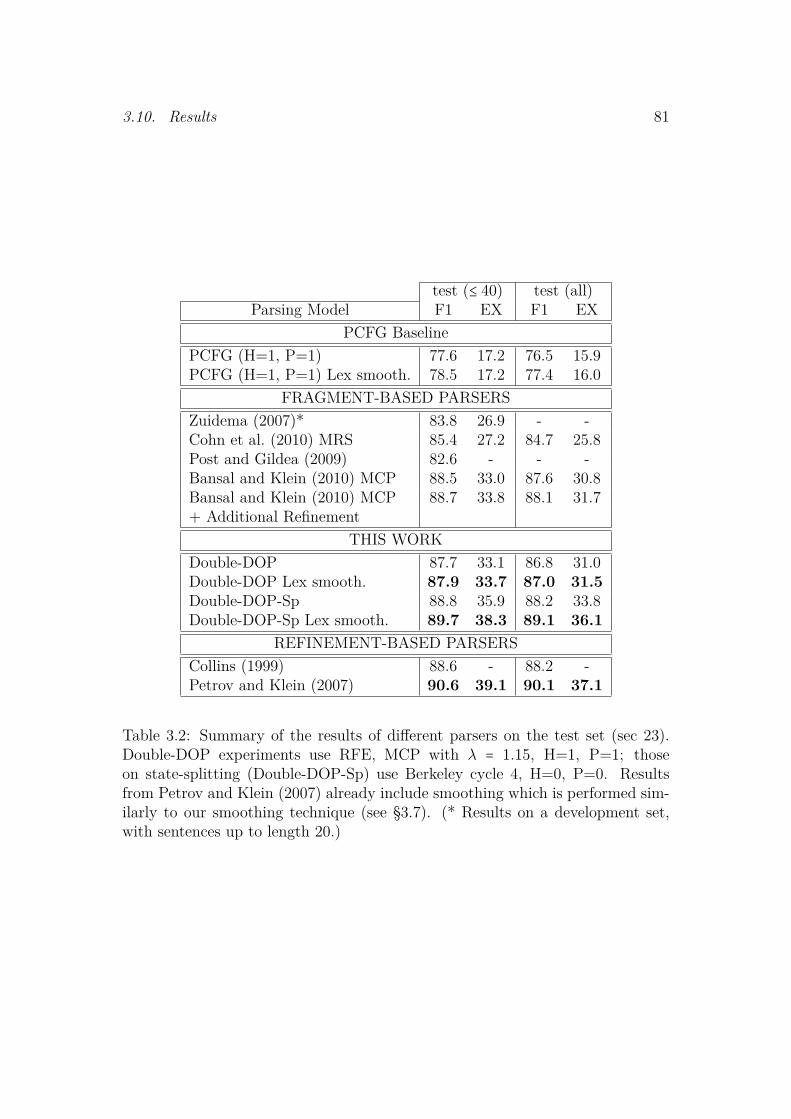
3.10. Results 81
test (≤ 40) test (all)Parsing Model F1 EX F1 EX
PCFG BaselinePCFG (H=1, P=1) 77.6 17.2 76.5 15.9PCFG (H=1, P=1) Lex smooth. 78.5 17.2 77.4 16.0
FRAGMENT-BASED PARSERSZuidema (2007)* 83.8 26.9 - -Cohn et al. (2010) MRS 85.4 27.2 84.7 25.8Post and Gildea (2009) 82.6 - - -Bansal and Klein (2010) MCP 88.5 33.0 87.6 30.8Bansal and Klein (2010) MCP 88.7 33.8 88.1 31.7+ Additional Refinement
THIS WORKDouble-DOP 87.7 33.1 86.8 31.0Double-DOP Lex smooth. 87.9 33.7 87.0 31.5Double-DOP-Sp 88.8 35.9 88.2 33.8Double-DOP-Sp Lex smooth. 89.7 38.3 89.1 36.1
REFINEMENT-BASED PARSERSCollins (1999) 88.6 - 88.2 -Petrov and Klein (2007) 90.6 39.1 90.1 37.1
Table 3.2: Summary of the results of different parsers on the test set (sec 23).Double-DOP experiments use RFE, MCP with λ = 1.15, H=1, P=1; thoseon state-splitting (Double-DOP-Sp) use Berkeley cycle 4, H=0, P=0. Resultsfrom Petrov and Klein (2007) already include smoothing which is performed sim-ilarly to our smoothing technique (see §3.7). (* Results on a development set,with sentences up to length 20.)

82 Chapter 3. Recycling Phrase-Structure Constructions
test (≤ 40) test (all)Treebank Parsing Model F1 EX F1 EXBrown PCFG 80.6 27.0 77.8 24.5
Berkeley Cycle 5 88.5 43.6 87.3 41.2Double-DOP 86.4 38.4 84.6 36.2
Negra PCFG 71.6 33.3 71.3 32.7Dubey (2005) 76.3 - - -Berkeley Cycle 4 78.9 42.3 78.5 41.6Double-DOP 76.5 40.2 76.0 39.5
FTB PCFG 76.0 16.3 72.7 12.8Arun and Keller (2005) 79.1 21.2 75.6 16.4Berkeley Cycle 5 84.2 26.1 82.2 20.8Double-DOP 81.5 21.1 78.7 16.6
CTB 3.0 PCFG 65.2 23.4 62.6 20.1Bikel (2004b) 81.2 - 79.0 -Berkeley Cycle 5 86.0 40.5 83.0 34.8Double-DOP 82.1 20.7 81.1 17.8
HTB PCFG 73.2 9.0 71.3 7.9Berkeley Cycle 5 81.4 15.7 80.0 13.9Double-DOP 77.9 13.8 75.8 12.1
Table 3.3: Parsing results on different treebanks: Brown (English), Negra (Ger-man), FTB (French), CTB (Chinese), and HTB (Hebrew).

3.11. Conclusions 83
3.11 ConclusionsWe have described Double-DOP, a novel DOP approach for parsing, which uses allconstructions recurring at least twice in a treebank. This methodology is drivenby the linguistic intuition that constructions included in the grammar shouldprove to be reusable in a representative corpus of annotated productions. Theextracted set of fragments is significantly smaller than in previous approaches.Moreover constructions are explicitly represented, which makes them potentiallygood candidates as semantic or translation units to be used in other applications.
Despite earlier reported excellent results with DOP parsers, they are almostnever used in other NLP tasks: where other successful parsers often feature ascomponents of machine translation, semantic role labeling, question-answering orspeech recognition systems, DOP is conspicuously absent in these neighboringfields (but for possible applications of closely related formalisms see, e.g., Bon-nema et al., 1997; Hearne and Way, 2006; Yamangil and Shieber, 2010). Thereasons for this are many, but most important are probably the computationalinefficiency of many instances of the approach, the lack of downloadable softwareand the difficulties with replicating some of the key results.
In this chapter we have addressed all three obstacles: our efficient algorithmfor identifying the recurrent fragments in a treebank runs in polynomial time, andthe transformation to PCFGs that we define allows us to use a standard PCFGparser, while retaining the benefit of explicitly representing larger fragments.Finally, the availability of our programs, as well as the third party software thatwe use, also addresses the replicability issue. Where some researchers in thefield have been skeptical of the DOP approach to parsing, we believe that ourindependent development of a DOP parser adds credibility to the idea that anapproach that uses very many large subtrees, can lead to very accurate parsers.
3.11.1 Future DirectionsThere is a number of extensions of the current model that are left unexplored.The set of recurring fragments used for parsing is rather big. Nevertheless thereis still a certain amount of fragments that occur only once in the training setwhich reoccur for the second time only in the development set. Some of these arestill relatively small fragments. It is then possible to augment our model with allor a random sample of small fragments that occurred only once in the trainingcorpus; this strategy might improve performance, while harming efficiency.
A more methodological variation of the model could come from the prepro-cessing of the treebank. One of the steps that were essential for the success of themodel was the binarization procedure. Binarization is particularly important forgenerative models like DOP and PCFGs, where all the daughters of an internalnode are produced at once. Binarization, in fact, provides a way to generalizeflat rules, by splitting it in multiple generation steps. In initial unpublished ex-
84 Chapter 3. Recycling Phrase-Structure Constructions
periments, our DOP model trained on an unbinarized treebank performed ratherpoorly because of the abundance of flat rules. However, our current model usesa strict left binarization (see §3.7). Although the practice of resorting to bi-narization techniques is often considered a mere heuristic for achieving higherparsing results, we would like to stress the fact that it is fundamental for solvingthe under-generation limitation of the underlying PCFG model; we believe moreeffort should be put into validating ways to perform this step.
Moreover, there is a number of probabilistic estimates that are left unexploredin our study. In particular, while our version of EM (see §3.6.3) tends to over-fitthe data as it tries to maximizes the likelihood of the training treebank, a moresensible approach would be to follow a cross-validation (CV) instantiation of EM(Zollmann and Sima’an, 2005; Mylonakis and Sima’an, 2008). According to EM-CV the training treebank is partitioned in several parts and EM is run on each ofthe partitions separately, although the frequency estimates of the fragments areaveraged over the EM-rounds to prevent over-fitting on the various partitions.
Finally, we believe that our algorithm for extracting recurring fragments couldbe beneficial in solving a number of linguistic tasks automatically, such as thedistinction between argument and adjuncts in a PS treebank (Villavicencio, 2002;Abend and Rappoport, 2010). In particular, a variation of our algorithm (Sangatiet al., 2010) is able to detect recurring partial-fragments, which are less restrictivethan the type of fragments used in this chapter: a partial-fragment can in factinclude any connected subset of nodes of the original tree, which allows to discardin a production any number of daughters. The use of partial-fragments couldgive also rise to yet another interesting parsing framework, where the argumentdaughters of a node (which are usually no more than 3) are produced in a singlestep, while adjuncts are inserted one at a time with a special-purpose insertionoperation (Schabes and Waters, 1995; Hwa, 1998; Bangalore et al., 2009) which isconstrained to apply on more restricted contexts (see also the “Sandwich InsertionGrammar” in example 2.2.6).
3.11.2 Next stepsAfter having described a novel DOP model for learning phrase-structure trees,in the next chapter we will turn our attention to dependency-based syntax. Asdescribed in §1.2.5 PS and DS are complementary representations focusing ontwo fundamental aspect of syntax, i.e., grouping and relations respectively. Thefragment-grammar we use in the Double-DOP model is able to capture a largepart of the relevant syntactic constructions, such as the argument structure ofmany lexical items, as well as a number of idiomatic expressions, but it is stronglybased on the notion of substitutability of internal phrasal categories. In thedependency-structure models, instead, we will focus on the direct relations ex-isting between words in a sentence, which Double-DOP is not able to captureconsistently.

Like the body that is made up of different limbs and organs,all words must depend on each other to exist.
Adaptation of an Hindu proverb
Chapter 4Learning Dependency-Structures
85
86 Chapter 4. Learning Dependency-Structures
4.1 IntroductionThe aim of this chapter is to introduce syntactic dependency-structures (DS), andcompare a number of computational models for obtaining the correct analysis ofnatural language sentences according to this representation.
We have decided to investigate dependency-structure, since it is a comple-mentary scheme with respect to phrase-structure representation employed in theprevious chapter. While PS trees are centered on abstract syntactic categories,and assign a rather marginal role to lexical productions, DS trees focus on wordsand on the direct dependency relations conntecting them.
Historically, the modern theoretical tradition of dependency-structures wasstarted by Lucien Tesniere (1959), who formulated this theory long before theformal notion of phrase-structure was proposed by Chomsky (1957).1 Never-theless, most of the initial formal studies on dependency-structure (Hays, 1960;Gaifman, 1965) were conducted only after phrase-structure was introduced, andwere presented mainly in relation to it.
We will dedicate chapter 5 to the description of a syntactic representationwhich is closer to the one described by Tesniere. There, we will show howTesniere’s theory incorporates aspects from both constituency and dependencytheories, and makes use of special constructions for handling common linguisticphenomena such as coordination, often neglected in other representations.
In the current chapter, we will limit our analysis to the description of sim-ple dependency-structure, where dependency is the only relation to link words ina sentence. This notion of DS is the one which was commonly adopted in thecomputational linguistics community in the ’90s, also thanks to the emergence ofhybrid models such as head-driven formalisms (Magerman, 1994; Collins, 1997,see also §3.2.1), which have strengthened the role that the lexicon plays in syn-tactic theories. Since then, DS received an increasing interest as an alternativerepresentation to the traditional PS.
After introducing the general notion of dependency-structure, we will describethe relation that exists between PS and DS, and how it is possible to transformone representation into the other. Finally we will present a family of generativemodels for learning DS, and show some results when parsing the Wall StreetJournal treebank using a reranking approach. The main motivation for usinga reranking approach is that it allows for efficiently evaluating many generativemodels, differing from one another on the hypothesis for how to derive the mostprobable structure for a given sentence. Although efficient algorithms exist tocalculate parse forests (e.g., Eisner and Satta, 1999), each choice gives rise to adifferent parser instantiation, while in our approach we can mimic the steps ofeach specific parser and employ a unique evaluation procedure (see also §2.4).
1In fact Elements de syntaxe structurale (Tesniere, 1959) was published posthumously(Tesniere died in 1954).

4.2. Dependency-Structure 87
4.2 Dependency-StructureA dependency-structure of a sentence is a tree structure whose nodes are thewords in the sentence. Differently from PS trees, where the order relation is onlydefined for a subset of nodes in the tree (e.g., the children of each node), all thenodes of a DS tree are in precedence relation to one-another (see the differencebetween figure 2.2 and 2.3). Precedence is implicitly defined by the order of thewords in the sentence.
Figure 4.1 shows an example2 of a DS. Edges indicate a dependency relationbetween the upper word, the governor (or head or parent) and the lower word,the dependent (or child). In figure 4.2 we report the same structure using anequivalent flat representation in which head-dependent relations are marked withdirected edges. The tree structure must be connected, and each must have exactlyone governor, except for the root node which has none.
VBDwore
NNPFrench
NNSbands
DTThe
NNPFree
JJblack
NNarm
Figure 4.1: Example of a dependency-structure according to the DS representa-tion used in this thesis.
DT NNP NNP VBD JJ NN NNSThe Free French wore black arm bands
Figure 4.2: Example of the dependency-structure in figure 4.1 using an equiva-lent flat representation. For every arc the arrow points at the dependent of thegovernor-dependent relation.
2In our DS trees we always report part-of-speech tags together with words, since both areused for parsing, and they should therefore be considered a unique entity (tagged word). InPS, instead, pos-tags rewrite to words at the bottom of each tree. See for comparison the PSof the same sentence in figure 3.1.

88 Chapter 4. Learning Dependency-Structures
The main conceptual difference between PS and DS is that a PS describespart-whole relations between constituents of a sentence, while a DS specifies theinterconnections between words, viz. the governing-dependency relations (seealso the discussion in §1.2.5).
In this chapter we will be focusing on projective DS, since our models willbe tested on the English WSJ treebank converted to projective DS.3 A DS isprojective iff for every word, the set including the word and all its direct andindirect dependents forms a continuous span of the sentence (without any hole).
Moreover, we will only consider unlabeled DS. A labeled DS, presents spe-cific tags on its arcs (e.g., subject, object, determiner, etc...) denominating thefunctional role that the dependent has with respect to the governor. These la-bels are useful as a further differentiation of the dependents of a certain word,and they can be used, for instance, for detecting the argument structure of verbs(who did what to whom) in parsing-related tasks (e.g., semantic role labeling).In our formalization we ignore these extra labels because we are mainly focusingon learning the bare structure of the sentence and for all the models we will dealwith, functional labels do not add any contribution for solving this task.
4.3 Comparing PS with DSIn this section we present a review some of the past studies that have attemptedto formally compare PS with DS. While in §4.3.1 we focus on the structuralrelations between the two representations, in §4.3.2 we describe previous attemptsof defining comparisons over grammar formalisms for the two schemes.
4.3.1 Structural relations between PS and DSHays (1960) presents a first comparison between PS and DS. In particular, heformalizes a correspondence between the two types of structure: each PS mapsto multiple DS, and each DS to one or more PS. Figure 4.3 shows these mappingsfor a generic sentence of 3 words. Here we have adopted a simplified notation:we omit the labels in the internal nodes of the PS and unary chains are avoided.In both representations part-of-speech tags are collapsed with words.
From the same figure it is immediately clear that there are more projectiveDS than PS for a given sentence. In both cases the number of structures growsexponentially in the length of the sentence,4 with DS consistently outnumbering
3Although non-projective conversion of the same treebank exists (Johansson and Nugues,2007) we have preferred to use more standard conversion procedures. It is commonly knownthat, compared to other languages, non-projective constructions in English are quite rareand mainly pertaining long-distance relations (e.g., wh-movement). For more details on non-projective DS and ways to parse them see Kuhlmann (2007).
4For a sentence of length n = {1, 2, 3, 4, 5, 6} we have {1, 1, 3, 11, 45, 197} PS trees and{1, 2, 7, 30, 143, 728} DS trees. The number of PS trees is given by the super catalan number

4.3. Comparing PS with DS 89
PS.
1 2
31 2 3
1
2 3
1
2
3
1
3
2
3
2
1
3
1
2
2
1 3
3
1 2
1
2 3
A B C D E F G
α β γ
Figure 4.3: Mappings between DS (in rectangles) and PS (in circles) with 3 words.Dashed lines indicate the mappings for which the number of constituents in thePS is equal to the number of the governors in the DS.
PS to DS For English, there is no significant treebank annotated in dependencyformat. In later experiments we will therefore resort to a transformation fromthe WSJ treebank into projective dependency representation. In order to performsuch transform we need to use the notion of head5 as introduced in section 3.2.1:for every non-terminal node in a PS we need to select a single daughter as thehead of the constituent. The following recursive procedure takes as input anhead-enriched PS tree rooted in node N and outputs the corresponding DS:
1. If N is a terminal PS node, it is transformed into a single terminal DS nodewith no dependents.
2. If N is a non-terminal node, all its daughters are transformed into DStrees (recursive step); those obtained from the non-head daughters becomedependent of the root of the DS obtained from the head daughter, followingthe same order as in the PS. For instance in figure 4.3 the leftmost PS (α)is mapped into the leftmost DS (A) if node 2 is chosen as the head of theconstituent (2 3) and 1 as the head of the whole tree.
sequence P (n) = 3(2n−3)P (n−1)−(n−3)P (n−2)/n, while the number of DS trees is obtainedas D(n) = C(3n + 1, n)/(n + 1), where C is the binomial coefficient, C(n, k) = n!/(k!(n − k)!).
5Interestingly, Hays (1960) does not refer to the notion of head in his formulation, but heindirectly refers to it as “the chosen” constituent for the transformation to apply.

90 Chapter 4. Learning Dependency-Structures
According to this conversion procedure, the number of DS trees that corre-spond to a given PS is determined by the different ways of assigning heads tothe internal nodes in the PS. This can be easily computed as the product of thenumber of daughters of each non-terminal node in the PS.
The reversed transformation (DS to PS) is more elaborate and less discussedin the literature. We report this procedure in Appendix B.1.
4.3.2 Relations between PS and DS grammarsContext-Free Grammars Gaifman (1965) defines a way to construct a DStree via Context Free Grammar rules (DS-CFG). This is similar to CFGs definedfor PS (see §1.3.1 and §2.2.2), except that, instead of using the rewriting sym-bol (→), parenthesis are used to distinguish the governor from the dependents.6Moreover, in order to preserve the linear order of words, rules use the star symbol(∗) to separate left and right dependents of a governing word.
In the general case, the system represents a word w with all its dependentsd1, d2, . . . , dk (k ≥ 1) as a single rule, i.e., w(d1, . . . , di,∗, di+1 . . . , dk), where wordw occurs in the sentence after word di and before di+1 (0 ≤ i ≤ k). If w hasno dependent (k = 0), it is represented as t(∗). Finally, if w is the root of thesentence, the rule ∗(w) is used. This notation has been adopted as a way tocompactly represent DS trees (see also Hays, 1964). For instance trees B, D, andF in figure 4.3 can be represented with the expression ∗(1(∗3(2∗))), ∗(2(1∗ 3)),and ∗(3(1(∗2)∗)) respectively.
In the same paper, Gaifman (1965) investigated the correspondences betweenPS-CFG and DS-CFG (see also Heringer, 1967; Schneider, 1998; Nivre, 2006).The work has been later on reformulated and extended by Robinson (1967). Themain result of these papers is the proof that for every PS-CFG there exists aweakly equivalent DS-CFG, and vice versa, i.e., the two grammars yield the sameset of sentences.7 Moreover two equivalent grammars would produce pairwise cor-responding trees according to the definition originally proposed by Hays (1960).
The idea of transforming a PS-CFG into an equivalent DS-CFG, althoughmethodologically sound, has never been adopted in real systems. One of themajor problems is that the resulting DS-CFGs are usually bigger than the originalone, especially for non-trivial PS-CFG presenting recursive rules.8 An examplethat shows this is presented in figure 4.4: while PS-CFG can compactly representrecursive rules, DS-CFG needs to encode all possible combinations explicitly.
6In fact, while in PS a node is made of (rewrites to) different daughter nodes, in DS a wordcannot be substituted by its dependents.
7An important condition for the mapping to exist is that the PS-CFG should be of finitedegree, i.e., for every category there must be an upper bound to the smallest number of successiverule applications in order to reach a terminal symbol.
8We are not aware of any formal or empirical study attempting to quantify such differences.

4.3. Comparing PS with DS 91
S
S
A B-H
S-H
C D-H
D
B C
A
PS-CFG DS-CFG
S→ S SS→ A BS→ C D
*(D)D(B C ∗)B(A ∗)A(*)C(*)*(B)B(D A ∗)D(C ∗)D(D C ∗)B(B A ∗)
(a) (b) (c)
Figure 4.4: Example of a PS (a) and a corresponding DS (b), according to thespecific head assignment marked with -H in (a). The table in (c) lists in the firstcolumn the PS-CFG rules extracted from the PS (a), and in the second columnthe weakly equivalent DS-CFG. In this example the DS-CFG rules are aboutthree times more numerous than the PS-CFG rules: the DS-CFG rules above theline are the ones necessary to encode the tree in (b), while the ones below the lineare needed to encode other trees, yielding for instance ABAB, CDCD, ABABCD.
In general, the application of CFG-rules and PS methodologies to dependency-structures had the unfortunate effect of overlooking most of the peculiarities whichare typical of dependency-structure. In particular, while PS notation defines anelegant way to compactly represent abstract syntactic rules (internal rewritingrules) that can be easily extended in a second moment to a particular choice ofa lexicon (terminal rules), DS cannot easily capture the notion of abstract rules,since the whole structure is defined at the lexicon level.
Projective Bilexical Dependency Grammars In the DS-CFG describedabove, all dependents of each word are produced at once. In a Projective Bilexi-cal Dependency Grammar (PBDG), instead, each dependency relation is treatedindividually. In this way the problem of finding a DS for a given sentence canbe formulated as finding the governor of each word, and assuring that the finalstructure is connected and projective. This approach has been shown to be moresuitable for learning dependency-structures, and will constitute the basic formal-ism when investigating generative models for DS in §4.5. PBDGs allow for agreater generalization with respect to DS-CFG. In fact, each word can be at-

92 Chapter 4. Learning Dependency-Structures
tached to any available governor,9 irrespectively of any other dependent attachedto it. This can be problematic for it allows, for instance, two objects to attachto a simple transitive verb. More sophisticated models define specific constraintsto alleviate this problem: usually, the choice of attaching a specific word as adependent of a certain node is conditioned on its previous dependents and on an-cestral information. PBDGs can be easily extracted from a corpus of annotatedDS trees. For instance in figure 4.5 we show the PBDG extracted from DS treein figure 4.1.
*root*
VBDwore
VBDwore
NNPFrench
VBDwore
NNSbands
NNPFrench
DTThe
NNPFrench
NNPFree
NNSbands
JJblack
NNSbands
NNarm
Figure 4.5: An example of Bilexical Dependency Grammar extracted from theDS tree in figure 4.1.
A study which clarifies the grammatical relations between PBDG and PS isthe work of Johnson (2007). It describes a series of Unfold-Fold proceduresto transform a Projective Bilexical Dependency Grammar (PBDG) into weaklyequivalent Context-Free Grammars. The main motivation behind this work is tomake available all known techniques developed for CFGs to PBDGs, includingthe possibility to use the standard CYK algorithm for parsing DSs according to aprojective bilexical generative model. These transformations are shown to mimicthe chart-parsing algorithm defined for PBDG in Eisner and Satta (1999).
4.4 Other related syntactic theoriesIn this section we briefly summarize some of the other existing syntactic theories.These, compared to standard DS, are characterized by having deeper and more
9A word should always look for an available governor to ensure projectivity. If, for instance,a model assigns governors of each word in the sentence in sequential order, G turns out to bean available governor for the current word W , if the span constituted by G and all its directand indirect dependents is adjacent to W .

4.4. Other related syntactic theories 93
complex representations, for which there is no significant amount of annotatedmaterial; they are therefore harder to study empirically. Other formalisms (e.g.,CCG) which have significant annotated resources derived either manually or au-tomatically from existing corpora are presented in §5.6, where we will comparethem with our TDS annotation scheme.
Lexical Functional Grammar (LFG)
Lexical Functional Grammar (Kaplan and Bresnan, 1982; Bresnan, 2000; Dal-rymple, 2001) is a linguistic theory that in contrast to other approaches assumestwo different levels of syntactic representation. It postulates a unique constituentstructure (c-structure), corresponding to the superficial phrase-structure tree. Inaddition it defines a functional level (f-structure) which is lexicalized and can bet-ter represent the argument structure of the sentence including possible variationin the surface position of the arguments. The two representations are related tothe PS and DS representations that are discussed in this thesis. However, LFGrepresentation is usually considered more deep and therefore harder to be derivedwith a computational model. Previous studies that have tested LFG for pars-ing have restricted the model to a manually defined LFG grammar (e.g., Riezleret al., 2002) or trained on a restricted treebank (e.g., Bod and Kaplan, 2003).
Head-driven Phrase-Structure Grammar (HPSG)
Head-driven Phrase-Structure Grammar (Pollard et al., 1994) is a formal linguis-tic theory based uniquely on feature structures (differently for instance from LFGwhich uses feature structure only within the functional representation). Eachfeature consists of an attribute and a value, where values can themselves be sub-features in a nested structure. Feature structures are used to represent grammarrules, principles, and lexical entries. As in LFG, HPSG is strongly lexicalized asthere is a small number of principles and grammar rules, while the lexicon is richand complex.
X-bar theory
X-bar theory (Harris, 1951; Chomsky, 1970; Jackendoff, 1977) is a theory fordescribing the relations between lexical and phrasal expressions of the same type(e.g., verb and verbal phrase). It can be seen as a hybrid approach between PS andDS as it captures the notion of head within phrase-structure.10 In his formulation,Chomsky (1970) proposes the phrase-structure scheme of figure 4.6, where Xranges among the main categories (Nouns, Verbs, Adjectives, Prepositions).
10See also Covington (1992) for more details on the interrelation between X-bar theory anddependency-structure.
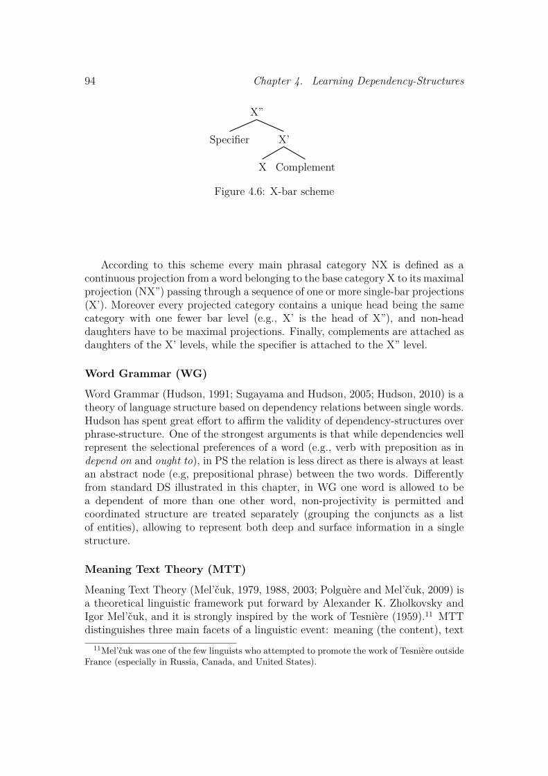
94 Chapter 4. Learning Dependency-Structures
X”
Specifier X’
X Complement
Figure 4.6: X-bar scheme
According to this scheme every main phrasal category NX is defined as acontinuous projection from a word belonging to the base category X to its maximalprojection (NX”) passing through a sequence of one or more single-bar projections(X’). Moreover every projected category contains a unique head being the samecategory with one fewer bar level (e.g., X’ is the head of X”), and non-headdaughters have to be maximal projections. Finally, complements are attached asdaughters of the X’ levels, while the specifier is attached to the X” level.
Word Grammar (WG)
Word Grammar (Hudson, 1991; Sugayama and Hudson, 2005; Hudson, 2010) is atheory of language structure based on dependency relations between single words.Hudson has spent great effort to affirm the validity of dependency-structures overphrase-structure. One of the strongest arguments is that while dependencies wellrepresent the selectional preferences of a word (e.g., verb with preposition as independ on and ought to), in PS the relation is less direct as there is always at leastan abstract node (e.g, prepositional phrase) between the two words. Differentlyfrom standard DS illustrated in this chapter, in WG one word is allowed to bea dependent of more than one other word, non-projectivity is permitted andcoordinated structure are treated separately (grouping the conjuncts as a listof entities), allowing to represent both deep and surface information in a singlestructure.
Meaning Text Theory (MTT)
Meaning Text Theory (Mel’cuk, 1979, 1988, 2003; Polguere and Mel’cuk, 2009) isa theoretical linguistic framework put forward by Alexander K. Zholkovsky andIgor Mel’cuk, and it is strongly inspired by the work of Tesniere (1959).11 MTTdistinguishes three main facets of a linguistic event: meaning (the content), text
11Mel’cuk was one of the few linguists who attempted to promote the work of Tesniere outsideFrance (especially in Russia, Canada, and United States).

4.5. Models for parsing DS 95
(the form), and a mapping between the set of meanings and the set of texts. Itincorporates several representation layers including semantics, syntax, morphol-ogy, and phonology. In the syntactic layer, MTT makes use of dependency treesin two different forms, i.e., deep and surface representation. The first specifiesthe organization of a sentence considered from the meaning frame of reference,while the latter is more connected to the surface form and therefore the actuallinear order of the words. While the inventory of the relations in the deep syn-tactic representation is supposed to be language-independent and related to theargument structure of the sentence (subject, object, complements), in the surfacesyntactic representation the relations are language specific, and the inventoryis established empirically. MTT deal with coordination structures by puttingeach element in the coordination (conjunction or conjunct) as the governor of thefollowing element (see also §5.3.3).
4.5 Models for parsing DSIn the following sections we will review some of the most relevant works on de-pendency parsing, distinguishing two main classes of models, i.e., generative anddiscriminative (see also section 2.5). Probabilistic generative dependency modelsdefine probability distributions over all valid dependency-structures. Discrimi-native models, instead, treat the problem of assigning the correct structure to agiven sentence as a classification task.
In recent evaluations of supervised dependency parsing (Buchholz and Marsi,2006; Nivre et al., 2007), generative approaches are consistently outperformedby discriminative models, on standard parsing evaluation metrics. On the otherhand, generative models provide a better way to investigate linguistic hypotheseson the derivation of syntactic structures.
4.5.1 Probabilistic Generative modelsProbabilistic Generative models for DS have played a minor role in computationallinguistics compared to their impact in PS representation. We believe that theyare still the most intuitive way to provide a formal account on how dependency-structures can be derived.
One of the most relevant existing studies concerning probabilistic generativemodels for DS is the work of Eisner (1996a,b), in which he proposes 4 probabilisticmodels (A, B, C, D) for DS parsing. The author makes use of a very efficientchart parsing algorithm (Eisner, 1997; Eisner and Satta, 1999; Eisner, 2000) forprojective dependency parsing whose complexity is O(n3) (where n is the lengthof the sentence), and it has a strict correspondence to the CKY algorithm appliedto the special transformation defined in Johnson (2007) (see §4.3.2).
Instead of relying on a chart parser, in our approach we decide to compare the

96 Chapter 4. Learning Dependency-Structures
4 generative models proposed by Eisner (1996a,b) using a reranking methodology(introduced in §2.4). In section 4.6 we will implement a more elaborated modelinspired by model C, and evaluate its performance on a standard evaluationbenchmark.
All the models (A,B,C,D) make use of two Markovian processes to generate theleft and right dependents of each node. In this process, dependents are generatedinside-outwards: those which are closer to the governor node are generated first.In order to make the model consistent, the two sequences of dependents need toterminate with a special symbol, i.e., the stop symbol ⊕ introduced in chapter 2(see also Collins models in §3.2.1). When the first left (or right) dependent isgenerated, the missing previously generated sibling is indicated with the nullsymbol ⊘. In three of the four models (A,B,D), a tagged sentence is generated inthe first phase as a sequence of ⟨word,pos-tag⟩ pairs. This sequence is generatedas a 2nd order Markovian process where every word (and its tag) is generated withprobabilities that depend on previous 2 words (and their tags). In our illustrationof those models we will skip the first phase and assume that a tagged sentence isalready given.
When describing the 4 models (A,C,B,D), we will refer to the example struc-ture illustrated in figure 4.7. The DS is rooted at the artificial node EOS (end ofsentence), conventionally put at the end of the sentence.
EOS
Vwon
NObama
Nelection
Dthe
Jpresidential
Figure 4.7: Dependency tree of the sentence “Obama won the presidential elec-tion”.
Model A For every word P in the sentence (from left to right), the model decideswhat are its left and right dependents, out of the list of the other taggedwords in the sentence. More specifically, for each word D present to theleft of P , the model decides whether or not D is a left dependent of P ,

4.5. Models for parsing DS 97
conditioned on the previously chosen dependent S (situated on the sameside). The same mechanism is done for the right dependents. For bothleft and right dependents, words in the sentence are examined from theone which is closest to P to the most remote one (inside-outwards). Moreconcisely the derivation of a structure can be described as a multiset of⟨event, conditioning-context⟩ pairs. A generic pair is described as follows:
⟨ YES/NO,D,left/right,P ,S , D,left/right,P ,S ⟩
Event: P has D as a left (right) dependent after S.Conditioning-context: D is to the left (right) of P in the sentence, and
S (or ⊘) is the previously chosen left (right) daughter of P .
Example: considering the structure in figure 4.7, the choice the modelperforms to decide that Obama-N is a left dependent of won-V is encodedin the ⟨event, conditioning-context⟩ pair
⟨ YES,Obama-N,left,won-V,⊘ , Obama-N,left,won-V,⊘ ⟩
where ⊘ specifies that there was no other left dependent of won-V beforeObama-N. Moreover, the fact that EOS is not a right dependent of won-Vis encoded as
⟨ NO,EOS,right,won-V,election-N , EOS,right,won-V,election-N ⟩
Model C According to this model, words are generated top-down starting fromthe artificial EOS symbol. For each node P under consideration, the modeldecides the full set of its left and right dependents as a Markovian process:each dependent D of P is chosen conditioned on P and on the previouslychosen left (right) dependent S. A generic ⟨event, conditioning-context⟩ paircan be described as:
⟨ D,left/right,P ,S , left/right,P ,S ⟩
Event: D is chosen as the left (right) dependent of P , and S (or ⊘) wasthe previously chosen left (right) dependent of P .
Conditioning-context: S (or ⊘) is the last chosen left (right) dependentof D and it has a following sister (or ⊕).
Example: in the structure of figure 4.7, the choice that Obama-N is a leftdependent of won-V is encoded as

98 Chapter 4. Learning Dependency-Structures
⟨ Obama-N, left, won-V,⊘ , left, won-V,⊘ ⟩
while the fact that election-N has no more left dependents after the-D isencoded as follows:
⟨ ⊕, left, election-N,the-D , left, election-N,the-D ⟩
Model B This model is identical to model C in defining the list of dependentsof each node. In addition, the model defines a further set of constraintsto allow each node to specify certain preferences on the node that governsit. Apart from the events generated from model C the new multiset of⟨event, conditioning-context⟩ pairs can be generically described as:
⟨ P ,D , D ⟩
Event: P is the parent node of D.Conditioning-context: D needs a parent node.
Example: in the structure of figure 4.7, the choice that Obama-N wantsas governor node won-V is encoded as
⟨ won-V,Obama-N , Obama-N ⟩
Model D The last model is again similar to model C, except that this time eachdependentD of a node P is selected from the words available in the sentence,conditioned on the previously chosen dependent S. More specifically D ischosen among the words which are to the left (right) of S in the sentence(plus the artificial node ⊕), or to the left (right) of P if S is ⊘ (no depen-dents have been chosen yet). This is substantially different from model C,since there the choice of D is made among the entire set of words includingthe ones not present in the sentence. A generic ⟨event, conditioning-context⟩pair can be generically described as:
⟨ D,left/right,P ,S , D,left/right,P ,S ⟩
Event: D is chosen as the left (right) dependent of P , following S (or ⊘).Conditioning-context: S is the last chosen left (right) dependent of P ,
and D is the ⊕ node or it is situated to the left (right) of S (or P ifS is ⊘) in the current sentence.

4.5. Models for parsing DS 99
Example: in the structure of figure 4.7, the choice that Obama-N is a leftdependent of won-V is encoded as
⟨ Obama-N, left, won-V,⊘ , Obama-N, left, won-V,⊘ ⟩
while the fact that election-N has no more left dependents after the-D isencoded as follows:
⟨ ⊕, left, election-N,the-D , ⊕,left, election-N,the-D ⟩
4.5.2 Discriminative modelsIn this section we will briefly review two standard approaches for dependency pars-ing using discriminative models: Maximum Spanning Tree (MST) and Transition-based models.
Maximum Spanning Tree
Maximum Spanning Tree (MST) models (McDonald et al., 2005; McDonald, 2006)efficiently keep track of all possible projective dependency-structures of a givensentence, and choose the one which maximizes a specific global function.
MST treats every dependency-structure as a multi-set of governor-dependentrelations. Each edge is described as an high dimensional feature vector. Forinstance, if in a certain DS word i is the governor of word j, v(i, j) is the vectordescribing all the features of this relation (i.e., labels of the two words, their pos-tags, and other information including e.g., words in between them, and ancestralnodes). During the training phase the model learns a weight vector w (having thesame dimension as v) which is then used to find the best dependency-structure yfor a given test sentence x. The score that needs to be maximized is defined as∑(i,j)∈y w ⋅ v(i, j), and the best candidate is called the Maximum Spanning Tree.
During the training phase the weight vector w is calculated in order to optimizethe scores of the tree structures in the training corpus. Roughly speaking, thealgorithm starts with a random weight vector, and iteratively updates the currentvector to a new one in order to reduce the number of errors it performs onpredicting the MST for each sentence in the training treebank, until an optimalweight is found. More specifically, the algorithm employs a large-margin classifier,which, for every structure y in the training treebank, tries to keep the score of yabove the scores of other incorrect structures of the same sentence by an amountwhich is proportional to how much they differ in accuracy.
For projective DS, both the training and parsing phase make use of a compactrepresentation of the tree forest. For this representation it is possible to useefficient dynamic programming algorithms for computing the best structure in

100 Chapter 4. Learning Dependency-Structures
cubic time as discovered by Eisner (1997, 2000). This also holds for a moreadvanced and accurate second-order model, in which two consecutive edges aretaken into consideration for each parsing decision, as opposed to a single edge inthe base case.
MST can also deal with labeled DS, but, in this case, labels are added ontop of the most probable DS of a given sentence as a separate task (also using adiscriminative classifier). Attempts of adding labels as features of the structuralmodel did not enhance performance on unlabeled dependency parsing. This isan important finding that justifies our choice of ignoring functional labels fordetecting the bare structure of a sentence.
Transition-based models
Transition-based models (Nivre, 2003; Yamada and Matsumoto, 2003), decom-pose the problem of obtaining the best dependency-structure of a given sentence,as a sequence of local decisions. An input sentence is read in one word at a time,and at each step a specific operation is performed.
These models are inspired by shift-reduce parsers, where a stack is used tokeep previously encountered words (partially connected) in a specific order. Theexact set of operations vary from model to model, but generally, it includes thereduce operation, to pop out a word from the stack, the shift operation, to pushthe current word onto the stack, and the attach operation, to draw dependencyrelations between the current word and the word on the top of the stack (in eitherdirections). Each operation can be applied only if certain conditions are met, toensure that the final DS is connected and projective.
In order to deal with non-projective structures, some transition-based modelsmake use of graph transformation (Nivre and Nilsson, 2005) as a second step orthey allow permutation operations over the words in the stack (Nivre, 2009).
Transition-based parser usually employ discriminative classifiers (e.g., SVM)in order to decide what is the best transition or sequence of transitions to apply.Each transition is described by a big set of feature, and the model parametersare learned from the training corpus using standard techniques.
The main difference with respect to the MST approach is that Shift-Reduceparsers are incremental (they accept one word at a time) and therefore attemptto learn optimal local decisions, while MST has a bigger scope since it aims atfinding the optimal structure as a whole.
4.6 Reranking generative modelsIn this section, we describe a reranking approach that combines a generative anda discriminative model and tries to retain the strengths of both. The idea ofcombining these two types of models through reranking is not new (see §2.5),

4.6. Reranking generative models 101
although it has been mostly explored in constituency parsing (Collins and Duffy,2002). This earlier work, however, used the generative model in the first step, andtrained the discriminative model over its k-best candidates. In our framework wereverse the usual order of the two models, by employing a generative model tore-score the k-best candidates provided by a discriminative model. Moreover, thegenerative model of the second phase uses frequency counts from the training setbut is not trained on the k-best parses of the discriminative model.
The reranking approach allows for efficiently evaluating many generative mod-els, differing from one another on (i) the choice of the linguistic units that are gen-erated (words, pairs of words, word graphs), (ii) the generation process (Markovprocess, top-down, bottom-up), and (iii) the features that are considered to buildthe event space (pos-tags/words, distance).
In our reranking perspective, all the generative model has to do is to computethe probability of k pre-generated structures, and select the one with maximumprobability. In a generative model, every structure can be decomposed into aseries of independent events, each mapped to a corresponding conditioning event.As an example, if a generative model chooses D as the right dependent of a certainword H, conditioned uniquely on their relative position, we can define the eventas D is the right dependent of H, and the conditioning event as H has a rightdependent.
As a preprocessing step, every sentence structure in the training corpus isdecomposed into a series of independent events, with their corresponding condi-tioning events. During this process, our model updates two tables containing thefrequency of events and their conditioning counterparts.
In the reranking phase, a given candidate structure can be decomposed intoindependent events (e1, e2, . . . , en) and corresponding conditioning events (c1, c2,. . . , cn) as in the training phase. The probability of the structure can then becalculated as
n
∏i=1
f(ei)f(ci)
(4.1)
where f(x) returns the frequency of x previously stored in the tables.12
It is important to stress the point that the only specificity each generativemodel introduces is in the way sentence structures are decomposed into events;provided a generic representation for the (conditioning) event space, both trainingphase and probability calculation of candidate structures can be implementedindependently from the specific generative model, through the implementation ofgeneric tables of (conditioning) events.
In this way the probabilities of candidate structures are exact probabilities,and do not suffer from possible approximation techniques that parsers often utilize(i.e., pruning). On the other hand the most probable parse is selected from the
12This probability estimate is the RFE introduced in §2.3.3.

102 Chapter 4. Learning Dependency-Structures
set of the k candidates generated by the discriminative model, and it will equalthe most probable parse among all possible structures, only for sufficiently highk.
4.6.1 Experiment SetupParser In order to generate a set of k-candidate structures for every test sen-tence, we use a state-of-the-art MST discriminative model13 (McDonald, 2006).The MST parser was provided with the gold standard pos-tags of the words inthe test set, and it was run in second-order and projective mode.
Treebank In our investigation, we have tested our model on the Wall StreetJournal corpus Marcus et al. (1993) with sentences up to 40 words in length,converted to dependency-structures. Although several algorithms exist to per-form such a conversion (e.g., Johansson and Nugues, 2007), we have followedthe scheme in Collins (1999). Section 2-21 was used as training, section 22 asdevelopment set, and section 23 as test set.
Evaluation Metrics As the only evaluation metric for dependency parsing wehave adopted the Unlabeled Attachment Score (UAS) (see Lin, 1995; Nivre et al.,2007), computed as:
UAS = # words with correct governor# words (4.2)
The root word of each parsed structure is considered to have the correctgovernor iff it is also the root of the sentence in the gold DS. The final UAS scoreis a macro-average over all the sentences in the test corpus.
4.6.2 Comparing the Eisner modelsWe have used the reranking framework just illustrated to compare the 4 generativemodels proposed by Eisner (1996a,b) presented in §4.5.1 on the development setof the WSJ. The results are shown in figure 4.8. All models show a progressivedecrease in performance as the number of best candidates increases. The resultsfor models B, C, and D are rather similar and consistently better than model A.This trend is consistent to the original results of Eisner (1996a,b) although modelC in our evaluation slightly outperforms the other two (in the original work modelD was the best performing one).
13The MST parser is available at http://sourceforge.net/projects/mstparser/.
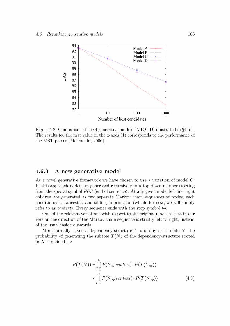
4.6. Reranking generative models 103
82
83
84
85
86
87
88
89
90
91
92
93
1 10 100 1000
UA
S
Number of best candidates
Model AModel BModel CModel D
Figure 4.8: Comparison of the 4 generative models (A,B,C,D) illustrated in §4.5.1.The results for the first value in the x-axes (1) corresponds to the performance ofthe MST-parser (McDonald, 2006).
4.6.3 A new generative modelAs a novel generative framework we have chosen to use a variation of model C.In this approach nodes are generated recursively in a top-down manner startingfrom the special symbol EOS (end of sentence). At any given node, left and rightchildren are generated as two separate Markov chain sequences of nodes, eachconditioned on ancestral and sibling information (which, for now, we will simplyrefer to as context). Every sequence ends with the stop symbol ⊕.
One of the relevant variations with respect to the original model is that in ourversion the direction of the Markov chain sequence is strictly left to right, insteadof the usual inside outwards.
More formally, given a dependency-structure T , and any of its node N , theprobability of generating the subtree T (N) of the dependency-structure rootedin N is defined as:
P (T (N)) =L
∏l=1P (N⪦l∣context) ⋅ P (T (N⪦l))
×R
∏r=1P (N⪧r∣context) ⋅ P (T (N⪧r)) (4.3)

104 Chapter 4. Learning Dependency-Structures
where L and R are the number of left and right children of N in T (L,R > 0), N⪦lis the left daughter of N at position l in T (analogously N⪧r for right daughters).The probability of the entire dependency-structure T is computed as P (T (EOS)).
In order to illustrate how a dependency-structure can be decomposed intoevents, we present in table 4.1 the list of events and the corresponding condition-ing events extracted from a toy treebank with two DS trees including the one infigure 4.7. In this simple example, each node is identified with its word, and thecontext is composed of the direction with respect to the governor, the governor,and the previously chosen daughter (or ⊘ if it is the first). While during thetraining phase the event tables are updated with these events, in the test phasethey are looked-up to compute the structure probability, as in equation 4.1.
Events Freq. Conditioning Events Freq.won L EOS ⊘ 1 L EOS ⊘ 2⊕ L EOS won 1 L EOS won 1⊕ R EOS ⊘ 2 R EOS ⊘ 2Obama L won ⊘ 1 L won ⊘ 1⊕ L won Obama 1 L won Obama 1election R won ⊘ 1 R won ⊘ 1⊕ R won election 1 R won election 1⊕ L Obama ⊘ 2 L Obama ⊘ 2⊕ R Obama ⊘ 2 R Obama ⊘ 2the L election ⊘ 2 L election ⊘ 2presidential L election the 1 L election the 2⊕ L election presidential 1 L election presidential 1⊕ R election ⊘ 2 R election ⊘ 2⊕ L the ⊘ 2 L the ⊘ 2⊕ R the ⊘ 2 R the ⊘ 2⊕ L presidential ⊘ 1 L presidential ⊘ 1⊕ R presidential ⊘ 1 R presidential ⊘ 1
Table 4.1: Events occurring when generating the dependency-structure in fig-ure 4.7, for the event space (dependent ∣ direction, governor, sister). The countsare extracted from a two-sentence corpus which also includes “Obama lost theelection”. According to the reported frequency counts, the structure has a asso-ciated probability of 1/4.
Model extension
In addition we have extended the model by including more contextual featuresand proper smoothing techniques for handling infrequent events and conditioningcontext.
In equation 4.3 we have generically defined the probability of choosing adaughter D based on specific features associated with D and the context in which

4.6. Reranking generative models 105
it occurs. In our implementation, this probability is instantiated as in equa-tion 4.4. The specific features associated with D are: the distance14 dist(H,D)between D and its governor H, the flag term(D) which specifies whether D hasmore dependents, and the lexical and postag representation of D. The context inwhich D occurs is defined by features of the governor H, the previously chosensister S, the grandparent G, and the direction dir (left or right).
In order to implement smoothing, equation 4.4 is factorized in four terms, eachemploying an appropriate backoff reduction list reported in descending priority.In the reduction lists, wt(N) stands for the string incorporating both the pos-tagand the word of N , and t(N) stands for its pos-tag. This second reduction isnever applied to closed class words. All the notation and backoff parameters areidentical to Eisner (1996a), and described in more details in Appendix B.2.
P (D∣context) = (4.4)P (dist(H,D), term(D),word(D), tag(D)∣H,S,G, dir) =P (tag(D)∣H,S,G, dir)
reduction list:
wt(H),wt(S),wt(G), dirwt(H),wt(S), t(G), dir
{ wt(H), t(S), t(G), dirt(H),wt(S), t(G), dir
t(H), t(S), t(G), dir× P (word(D)∣tag(D),H,S,G, dir)
reduction list: wt(H), t(S), dirt(H), t(S), dir
× P (term(D)∣word(D), tag(D),H,S,G, dir)
reduction list: tag(D),wt(H), t(S), dirtag(D), t(H), t(S), dir
× P (dist(P,D)∣term(D),word(D), tag(D),H,S,G, dir)
reduction list: word(D), tag(D), t(H), t(S), dirtag(D), t(H), t(S), dir
4.6.4 ResultsResults for the development set are reported in table 4.9, as unlabeled attach-ment score (UAS). The MST dependency parser obtains very high results whenemployed alone (92.58%), and generates a list of k-best-candidates which canpotentially achieve much better results (an oracle would score above 95% when
14In our implementation distance values are grouped in 4 categories: 1, 2, 3 − 6, 7 −∞.

106 Chapter 4. Learning Dependency-Structures
k-best Oracle best Oracle worst Reranked1 92.58 92.58 92.582 94.22 88.66 92.893 95.05 87.04 93.024 95.51 85.82 93.025 95.78 84.96 93.026 96.02 84.20 93.067 96.23 83.62 93.098 96.40 83.06 93.029 96.54 82.57 92.9710 96.64 82.21 92.96100 98.48 73.30 92.321000 99.34 64.86 91.47
91.00%
92.00%
93.00%
94.00%
95.00%
96.00%
97.00%
98.00%
99.00%
100.00%
1 2 3 4 5 6 7 8 9 10 100 1000
Oracle-Best
Reranked
MST
Figure 4.9: UAS accuracy of the MST discriminative and reranking parser onsection 22 of the WSJ. Oracle best: always choosing the best result in the k-best,Oracle worst: always choosing the worst, Reranked: choosing the most probablecandidate according to the generative model.
Error reduction analysis between the reranked 7-best
and the MST 1-best
NN
NNP
IN
DT
NNS
JJ
,
. VBD
CD
RB
CC
VB
VBN
TO
VBZ
PRP
VBG
POS
VBP
$
MD
PRP$
`` '
: WDT
JJR
RP
RBR
WRB WP
JJS
-60%
-50%
-40%
-30%
-20%
-10%
0%
10%
20%
30%
40%
NN
NNP
IN DT
NNS JJ
, .
VBD
CD
RB
CC
VB
VBN
TO
VBZ
PRP
VBG
POS
VBP $
MD
PRP$
`` ' :
WDT
JJR
RP
RBR
WRB
WP
JJS
Erro
r R
ed
ucti
on
0%
3%
6%
9%
12%
15%
18%
21%
24%
27%
30%
Rela
tive f
req
uen
cy
0%
3%
6%
9%
12%
15%
Figure 4.10: Error reduction analysis between the reranked 7-best and the MST1-best on the different pos-tags (above), and relative frequencies of the variouspos-tags in the test set (below).
4.7. Conclusions 107
selecting from the first 5-best, and above 99% from the first 1000-best). Thedecrease in performance of the generative model, as the number of the candidateincreases, suggests that its performance would be lower than a discriminativemodel if used alone. On the other hand, our generative model is able to selectbetter candidates than the MST parser, when their number is limited to a fewdozens, yielding a maximum accuracy for k = 7 where it improves accuracy on thediscriminative model by a 0.51% (around 7% error reduction). In figure 4.10 wepresent a per-category analysis on the error reduction of our best results comparedto those of the MST parser.
We have evaluated the performance of the same model on the test set ofthe WSJ (sec 23), when reranking the 7-best candidates provided by the MSTparser. The improvement here is smaller (0.11%: from 92.42% of the MST parserto 92.53%) but proves that the model is robust when reranking a restricted setof candidates.
4.7 ConclusionsIn this chapter we have presented the notion of dependency-structure, and com-pared it with phrase-structure representation. Overall, the two representationscan be considered as two ways to represent syntactic structures from two differentperspectives: while PS defines a recursive way to group words of a sentence intoconstituents, DS specifies what are the dependency relations between words in asentence.
The main contribution of this chapter was to propose a general frameworkfor dependency parsing based on a combination of discriminative and generativemodels. We have used this framework to evaluate and compare several gener-ative models, including those of Eisner (1996b) and some of their variations.Consistently with earlier results, none of these models performs better than thediscriminative baseline when used alone. We have presented an instantiation ofthis framework in which our newly defined generative model leads to an improve-ment of the state-of-the-art parsing results, when provided with a limited num-ber of best candidates. This result suggests that discriminative and generativemodel are complementary: the discriminative model is successfully at filteringout “bad” candidates, while the generative model is able to further refine theselection among the few best candidates. In our set-up it is now possible to ef-ficiently evaluate many other generative models and identify the most promisingones for further investigation. Given the abundance of discriminative models fordependency parsing (Nivre, 2003; McDonald, 2006), our promising results showthat generative models can still produce competitive results and therefore thepessimism about the prospects of probabilistic generative dependency models ispremature.

108 Chapter 4. Learning Dependency-Structures
4.8 Future DirectionsIn §1.2 we have illustrated how the syntactic domain, which is the main focus ofthe thesis, does not account for the full spectrum of phenomena which should beregarded when processing natural language expressions. In particular, althoughmuch work has supported the independence between syntax and semantic process-ing (Jackendoff, 2002), there is empirical evidence about the benefit of combinedmodels for obtaining better disambiguation (Mitchell and Lapata, 2009). In par-ticular, many mistakes of state-of-the-art parsers are on preposition attachment,and relying on semantical preferences of verbs and nouns could help to solve a bignumber of those ambiguities. The possibility of combining syntactic and seman-tics models could also contribute to shedding light on the opposite interconnectionbetween the two domains. Current distributional semantics models are usuallyuninformed about the syntax underlying the set of sentences used for training.It would be therefore interesting to study how syntax can provide useful clues toobtain better semantic space models.
All parsing models that we have developed in this chapter were trained onthe WSJ treebank which is relative small and domain-specific. The main short-coming for this is that, although our DS models heavily rely on direct dependencyrelations between lexical items, they are quite restricted to work with a ratherconcise vocabulary. Possible extensions of our models could attempts to overcomethis limitation by relying on semi-supervised learning techniques, in which themodels can obtain additional information from surface counts extracted fromlarge unannotated corpora such as the web (Lapata and Keller, 2004; Bansal andKlein, 2011).
Finally, in chapter 3 we have described an efficient algorithm for extract-ing all arbitrarily large syntactic constructions which occur multiple times in alarge treebank. Although our implementation is specific for PS treebanks, itwould not be difficult to extend it to the DS representations. In particular ina dependency-structure treebank it would be interesting to detect all recurringpartial-fragments, i.e., any connected subset of nodes recurring in several trees ofa treebank (Sangati et al., 2010). These constructs could be useful for derivingnovel generative models for parsing DS.
On peut ainsi comparer le verbe a une sorte d’atome crochususceptible d’exercer son attraction sur un nombre plus oumoins eleve d’actants, selon qui’il comporte un nombre plus oumoins eleve de crochets pour les maintenir dans sa dependance.Le nombre de crochets que presente un verbe et par consequentle nombre d’actants qu’il est susceptible de regir, constitue ceque nous appellerons la valence du verbe.
We can also compare the verb to a sort of atom with hookscapable of exerting an attraction force on a certain number ofelements, by means of an equal number of hooks which allow theatom to keep them under its dependence. The number of hooksof a verb and consequently the number of elements it is able togovern, constitute what we will call the valence of the verb.
Lucien Tesniere (1959, p.238)
Chapter 5Tesniere Dependency-Structure
109

110 Chapter 5. Tesniere Dependency-Structure
5.1 IntroductionAfter having described in the previous two chapters syntactic models for learn-ing phrase-structure and dependency-structure, in this chapter we introduce anovel syntactic representation that includes aspects from both PS and DS. Thenew representation was strongly inspired by the general theory of dependencysyntax formulated by Lucien Tesniere (1959). Recent projects aiming at rein-forcing the role of DS representation in computational linguistics (e.g., Yamadaand Matsumoto, 2003; Forst et al., 2004; Johansson and Nugues, 2007) typicallyrefer to Tesniere as the father of dependency syntax, but little attempt has beenmade to explain how the chosen dependency representation relates to the originalwork. A careful comparison reveals substantial differences: modern DS retainsonly the main idea proposed by Tesniere, namely the relation of dependency be-tween words (§5.2.1), while other operations and features of the original theoryare discarded or not overtly represented.
In this chapter we propose a formalization of Tesniere’s theory, and derive anautomatic conversion of the English Wall Street Journal Treebank into a novelrepresentation: the Tesniere Dependency-Structure (TDS). This work is based ona joint collaboration with Chiara Mazza (i.e., Sangati and Mazza, 2009).
The current chapter is structured as follows: In §5.2 we retrace the originalwork by Tesniere and introduce the newly proposed TDS representation. In par-ticular we reintroduce three key concepts: the division of a sentence into blocksof words, which act as intermediate linguistic units (§5.2.2), the junction oper-ation, to handle coordination and other types of conjoined structures (§5.2.3),and the operation of transference, to generalize over the categories of the lin-guistic elements (§5.2.4).1 In §5.3 we give empirical evidence that shows howthis representation can incorporate all main advantages of modern PS and DS,while avoiding well known problems concerning the choice of heads and betterrepresenting common linguistic phenomena such as coordination. In §5.4 we de-scribe the procedure used to convert the WSJ into TDS notation, and in §5.5we propose a novel generative model for parsing the TDS treebank, and utilize areranking framework for testing it. We also introduce a novel evaluation schemefor measuring the accuracy of the generated parse trees, focusing on the 3 maincomponents of the TDS scheme: blocks, dependency, and coordination. Finally,in §5.6 we compare the TDS conversion with other proposed conversions of theWSJ treebank. In particular in §5.7 we report on a detail comparison betweenthe TDS-bank and the CCG-bank (Hockenmaier and Steedman, 2007) focusingon the detection of coordination constructions.
1See in Tesniere (1959) part I ch. 22 on nucleus, part II on jonction, and part III ontranslation. We choose transference for the original French word translation to avoid any mis-understanding with the other meaning of the word translation in English. Unfortunately, 50years after its publication, there is still no English translation of the author’s work, yet thereis for Russian, German, and Italian.
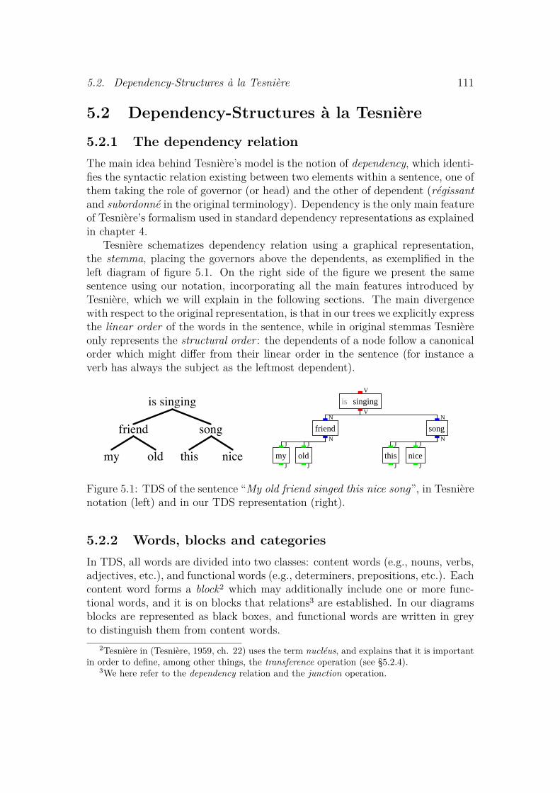
5.2. Dependency-Structures a la Tesniere 111
5.2 Dependency-Structures a la Tesniere
5.2.1 The dependency relationThe main idea behind Tesniere’s model is the notion of dependency, which identi-fies the syntactic relation existing between two elements within a sentence, one ofthem taking the role of governor (or head) and the other of dependent (regissantand subordonne in the original terminology). Dependency is the only main featureof Tesniere’s formalism used in standard dependency representations as explainedin chapter 4.
Tesniere schematizes dependency relation using a graphical representation,the stemma, placing the governors above the dependents, as exemplified in theleft diagram of figure 5.1. On the right side of the figure we present the samesentence using our notation, incorporating all the main features introduced byTesniere, which we will explain in the following sections. The main divergencewith respect to the original representation, is that in our trees we explicitly expressthe linear order of the words in the sentence, while in original stemmas Tesniereonly represents the structural order : the dependents of a node follow a canonicalorder which might differ from their linear order in the sentence (for instance averb has always the subject as the leftmost dependent).
is singing
friend song
my old this nice my old
friend
is singing
this nice
song
J
J
J
J
N
N
V
V
J
J
J
J
N
N
Figure 5.1: TDS of the sentence “My old friend singed this nice song”, in Tesnierenotation (left) and in our TDS representation (right).
5.2.2 Words, blocks and categoriesIn TDS, all words are divided into two classes: content words (e.g., nouns, verbs,adjectives, etc.), and functional words (e.g., determiners, prepositions, etc.). Eachcontent word forms a block2 which may additionally include one or more func-tional words, and it is on blocks that relations3 are established. In our diagramsblocks are represented as black boxes, and functional words are written in greyto distinguish them from content words.
2Tesniere in (Tesniere, 1959, ch. 22) uses the term nucleus, and explains that it is importantin order to define, among other things, the transference operation (see §5.2.4).
3We here refer to the dependency relation and the junction operation.

112 Chapter 5. Tesniere Dependency-Structure
Tesniere distinguishes four block categories (or functional labels4), here listedtogether with the color and single letter notation, as reported in our diagrams:nouns (blue, N), adjectives (green, J), verbs (red, V), and adverbs (yellow, A).
Dependency relations are defined upon blocks. The verbal block representsthe process expressed by the clause, and each of its arguments, representing aparticipant in the process, functions as a single noun. Arguments are usuallycompulsory within the clause, and their number is determined by the verb’s va-lence. On the other hand the verb’s adjuncts (or circonstants), represent thecircumstances under which the process is taking place, i.e., time, manner, loca-tion, etc., and function as adverbs.
Tesniere was the first linguist borrowing the term valency from chemistry, toindicate the number of ‘empty slots’ that a verb should fulfill. So for instanceintransitive verbs such as to sleep has valency 1 in ‘the dog sleeps’, since thesubject is the only compulsory argument, while to give has valency 3 in ‘he givesher a book’.
Nouns are always modified by blocks that function as adjectives, and adjectivesby blocks that function as adverbs.
We will now introduce two operations, junction and transference, which allowto construct more complex clauses from simple ones.
5.2.3 JunctionThe first operation is the junction and it is used to group elements that arecoordinated in a sentence. As in the dependency relation, junction acts overblocks. In this case blocks are called the conjuncts, and are grouped into aunique entity which has the status of a block (a junction block). The conjunctsare horizontally connected in the TDS, belong to the same category, and areoptionally connected by means of functional words, the conjunctions. In ourTDS diagrams junction blocks are displayed in yellow to distinguish them fromstandard block (black). Conjunction words (or punctuation marks functioning assuch) are also displayed in yellow.
Figure 5.2 displays three coordinated structures: in the first case, two nouns,subject of the same verb, are coordinated; in the second case, two adjectives,modifying the same noun, are coordinated; in the last case, two verbs, havingthe same subject, are coordinated. As in Tesniere’s formulation, we use junctionto represent standard coordination as well as apposition (e.g., [the US president],[Obama]). Moreover, the junction operation can work recursively: a junctionblock can be a conjunct of a bigger junction block (e.g., [Mary and [either Markor John]]).
4We will use both terms interchangeably. Categories can be roughly seen as a simplificationof both PoS tags and dependency relations in DS’s. See also §5.3.2.
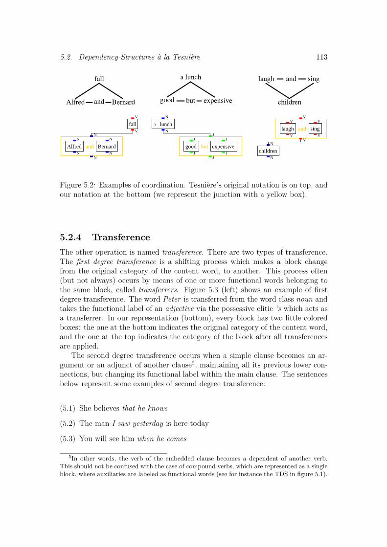
5.2. Dependency-Structures a la Tesniere 113
fall
Alfred and Bernard
a lunch
good but expensive
laugh and sing
children
Alfred and Bernard
fall
N
N
N
N
N
N
V
V
a lunch
good but expensive
N
N
J
J
J
J
J
J children
laugh and sing
N
N
V
V
V
V
V
V
Figure 5.2: Examples of coordination. Tesniere’s original notation is on top, andour notation at the bottom (we represent the junction with a yellow box).
5.2.4 TransferenceThe other operation is named transference. There are two types of transference.The first degree transference is a shifting process which makes a block changefrom the original category of the content word, to another. This process often(but not always) occurs by means of one or more functional words belonging tothe same block, called transferrers. Figure 5.3 (left) shows an example of firstdegree transference. The word Peter is transferred from the word class noun andtakes the functional label of an adjective via the possessive clitic ’s which acts asa transferrer. In our representation (bottom), every block has two little coloredboxes: the one at the bottom indicates the original category of the content word,and the one at the top indicates the category of the block after all transferencesare applied.
The second degree transference occurs when a simple clause becomes an ar-gument or an adjunct of another clause5, maintaining all its previous lower con-nections, but changing its functional label within the main clause. The sentencesbelow represent some examples of second degree transference:
(5.1) She believes that he knows
(5.2) The man I saw yesterday is here today
(5.3) You will see him when he comes
5In other words, the verb of the embedded clause becomes a dependent of another verb.This should not be confused with the case of compound verbs, which are represented as a singleblock, where auxiliaries are labeled as functional words (see for instance the TDS in figure 5.1).
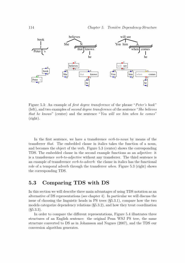
114 Chapter 5. Tesniere Dependency-Structure
book
PeterJ's
he
believes
She Nthat knows
You Awhen comes
he
him
will see
Peter 's
book
J
N
N
N She
believes
that
he
knows
N
N
V
VN
VN
N
You
will see
him when
he
comes
N
N
V
VN
N
A
VN
N
Figure 5.3: An example of first degree transference of the phrase “Peter’s book”(left), and two examples of second degree transference of the sentence “She believesthat he knows” (center) and the sentence “You will see him when he comes”(right).
In the first sentence, we have a transference verb-to-noun by means of thetransferrer that. The embedded clause in italics takes the function of a noun,and becomes the object of the verb. Figure 5.3 (center) shows the correspondingTDS. The embedded clause in the second example functions as an adjective: itis a transference verb-to-adjective without any transferrer. The third sentence isan example of transference verb-to-adverb: the clause in italics has the functionalrole of a temporal adverb through the transferrer when. Figure 5.3 (right) showsthe corresponding TDS.
5.3 Comparing TDS with DSIn this section we will describe three main advantages of using TDS notation as analternative of DS representations (see chapter 4). In particular we will discuss theissue of choosing the linguistic heads in PS trees (§5.3.1), compare how the twomodels categorize dependency relations (§5.3.2), and how they treat coordination(§5.3.3).
In order to compare the different representations, Figure 5.4 illustrates threestructures of an English sentence: the original Penn WSJ PS tree, the samestructure converted to DS as in Johansson and Nugues (2007), and the TDS ourconversion algorithm generates.

5.3. Comparing TDS with DS 115
S
NP-SBJ
NNP-H
Japan
VP-H
CONJP
RB-H
not
RB
only
VP
VBZ-H
outstrips
NP
DT
the
NNP-H
U.S.
PP-LOC
IN-H
in
NP
NN
investment
NNS-H
flows
CONJP-H
CC-H
but
RB
also
VP
VBZ-H
outranks
NP
PRP-H
it
PP-LOC
IN-H
in
NP
NP-H
NN-H
trade
PP-CLR
IN-H
with
NP
JJS
most
JJP
JJ
Southeast
JJ-H
Asian
NNS-H
countries
.
.
SBJNNPJapan
CCRBnot
DEPRB
only
COORDVBZ
outstrips
NMODDTthe
OBJNNPU.S.
ADVINin
NMODNN
investment
PMODNNSflows
ROOTCCbut
COORDRBalso
COORDVBZ
outranks
OBJPRP
it
ADVINin
PMODNN
trade
ADVIN
with
NMODJJS
most
AMODJJ
Southeast
NMODJJ
Asian
PMODNNS
countries
P..
Japan
not only outstrips
the U.S. in
investment
flows
but also outranks
it in trade
with
most
Southeast
Asian
countries
.
N
N
V
V
V
VN
N
A
NJ
N
V
VN
N
A
NJ
NJ
JA
J
J
J
Figure 5.4: Comparison between different representations of an English sentence.Top: original WSJ PS taken from the WSJ sec-00 (#666). Null productions andtraces have been removed. The red labels are the heads according to the DS below.Center: DS according to Johansson and Nugues (2007) using the pennconverterscript in conll2007 mode. Every word in the DS is presented together with itsPoS and the label of the dependency relation with its governor. Bottom: TDSour conversion algorithm generates.

116 Chapter 5. Tesniere Dependency-Structure
5.3.1 Choosing the correct headsAs for DS, the easiest way to construct a TDS tree is to derive it automaticallyfrom a PS tree. A fundamental operation that both DS and TDS transformationhave in common is the annotation of the original PS tree with head labels (seealso §3.2.1 and §4.3.1). This procedure has been initially proposed by Magerman(1994) and then slightly modified by others (e.g., Collins, 1999; Johansson andNugues, 2007). If exactly one unique head is chosen for every constituent of thePS, the enriched tree can be shown to be homomorphic to a single projectiveDS (Hays, 1960; Nivre, 2006). For example, in figure 5.4, the DS in the center isderived from the heads marked with suffix -H in the PS at the top of the samefigure.
Choosing heads in a PS tree is a critical operation: although much linguisticliterature is present on this issue (cf. Corbett et al., 2006), in NLP there havebeen only few attempts to empirically evaluate different heads assignments (i.e.,Chiang and Bikel, 2002; Sangati and Zuidema, 2009). While certain choices areless disputed (e.g., the verb is unequivocally the head of simple clauses), themajority of the decisions are more controversial and they are usually betweenfunctional and content words. The most frequent cases are listed here:
• Determiner vs. noun in nominal phrases (e.g., the man).
• Preposition vs. noun in prepositional phrases (e.g., on paper).
• Complementizer vs. verb in sub-clauses (e.g., I believe that it is raining).
In TDS, all these choices become irrelevant: since every functional word isincluded in the block together with the content word it belongs to, both decisionslead to the same TDS representation. Nevertheless, in TDS, head assignmentremains essential when two or more content words are sister nodes of the sameconstituent, such as in “the song which I like”. For these cases there is moreconsensus about the choice of the heads: in the example the verb is consistentlymarked as the head of the subclause,6 and in our representation we follow thisconvention.
5.3.2 Categories and BlocksCurrently used DS representations make use of labels to identify the dependenciesbetween words. For example SBJ and OBJ are used to mark the relation betweena verb and its subject and direct object respectively, while NMOD is used toidentify the role of a noun modifier (i.e., adjective). These labels are only partially
6For these cases few people, such as Bauer (1979), have proposed that the subject couldalso be the head of the sentence. For more discussion on this issue see also Anderson (1971)and Vater (1975).
5.3. Comparing TDS with DS 117
overlapping with the four categories proposed by Tesniere as for instance noun-phrases are marked as nouns regardless of their role with respect to the verb ofthe sentence (e.g., subject or object). Moreover, while DS uses around a dozen ofdifferent labels, TDS uses only four. This turns out to be beneficial for a moresimplified and generalized analysis.
The other difference is more subtle. In DS every word is a node, and therefore,for every node (except for the root) there is the need to identify the label of thedependency relation with its governor. The problem here is related to the abovediscussion about the choice of heads. If we take the example in figure 5.3 (center),one has to choose whether the complementizer or the verb is the direct object ofthe main verb. TDS better represents these cases, by including both elements inthe same block. This choice is justified by the fact that both elements contributeto making the node an argument or an adjunct of the verb.
5.3.3 CoordinationCoordination is a very productive phenomenon in language. In the WSJ almostevery other sentence presents a coordination structure. Unfortunately coordi-nation represents one of the major problems in standard DS representation (seeNivre, 2006, p. 49). If dependency7 is the only operation available to relate words,two main strategies are adopted, leading to 4 possible annotation schemes:
1. One conjunction (or conjunct) is the head of the other elements.
2. Each element (conjunction or conjunct) is the head of the adjacent elementwhich follows.
The first solution is the one which is more commonly adopted in current PS-to-DS conversions. The second one is proposed by Igor Mel’cuk (1988). Bothsolutions are problematic in circumstances such as the one of figure 5.4 (seealso figure 5.9). If the coordination includes multiple conjunctions, assigning thehead to either one of the conjuncts or one of the conjunctions, leads to a strongasymmetry in the structure: either the conjuncts are not all at the same level, orthe set of dependents includes both conjunctions and conjuncts. Moreover, if thecoordination phrase is coordinating verbs at the top of the sentence structure,other potential blocks, e.g., the subject Japan in the example, will also appear inthe set of dependents, at the same level with the verbs they depend on.8 Finallythe conjunction phrase, i.e., a group of words forming a single conjunction (e.g.,
7We only consider the case of single headed DS, i.e., each word should have exactly onegovernor.
8The labels of the dependency relations, such as the ones in the DS of figure 5.4, can oftenhelp to differentiate between dependents which have the same head, but differ in their functionallabels. However they cannot be considered an optimal solution, since they do not eliminate thestructural asymmetry.

118 Chapter 5. Tesniere Dependency-Structure
not only in the example), is also poorly represented in DS representations, sinceit is not grouped into a unique entity.
Tesniere’s choice of adding a special operation to handle coordination is jus-tified if we consider how well it represents all the cases DS fails to describe con-sistently. Coordination in TDS can be seen as a borrowing of the notion ofconstituency from PS notation: the different blocks being conjoined have equalstatus, they govern all the blocks being dominated by the coordination block, andare dependents of all blocks the coordination structure depends on.
5.4 Converting the Penn WSJ in TDS notationWe will now present our attempt of converting the Penn WSJ treebank (Marcuset al., 1993) into TDS notation. In §5.4.1 we will introduce the elements com-posing each generated TDS, in §5.4.2 we will describe the conversion procedure,and in §5.6 we will compare the obtain treebank to other formalisms.
5.4.1 Elements of a TDSFigure 5.5 illustrates the main elements, introduced in §5.2, which we need todefine in order to construct TDS trees. Words are divided into content andfunctional words,9 and blocks are either standard or junction blocks. A genericblock contains a list of functional words, and a list of dependent blocks. Inaddition a standard block has to contain a unique content word,10 while a junctionblock needs to specify a list of conjunction words and a list of conjunct blocks.
Word { {Standard Block
- Content Word (CW)
Junction Block
- Conjunctions (FW) - Conjuncts (Block)
Block- Functional Words (FW) - Dependents (Block)
Functional Word (FW)
Content Word (CW)
Figure 5.5: Hierarchical definition of words and block types in the TDS represen-tation.
9A word is functional if its PoS is one of the following: punctuation marks, CC, DT, EX,IN, MD, POS, RP, SYM, TO, WDT, WRB. Moreover special pairs of words are marked asfunctional (e.g., more like, more than, even though, such as, many of, most of, rather than).
10As the only exception, contiguous proper nouns (e.g., first and last names) are parts of thesame block.

5.4. Converting the Penn WSJ in TDS notation 119
5.4.2 The conversion procedureIn order to derive TDS trees from the Penn WSJ, we have decided to start fromthe original PS annotation, instead of using already converted DS trees. The mainreason for this choice is that PS annotation of the WSJ is richer than currentlyavailable DS representations. This concerns in particular coordination structures,which would be much harder to reconstruct from DS notation (see §5.3.3).
Each PS in the corpus is preprocessed using the procedure described in Vadasand Curran (2007), in order to add a more refined bracketing structure to nounand adjectival phrases. Moreover, we remove null productions and traces fromall trees, and enrich them with head labels. This last step is performed usinga variation of the head-rules table defined in Magerman (1994) as reported inAppendix C.1.
Conversion
The pseudocode reported in algorithm 2, contains the procedure which is appliedto each PS of the corpus, in order to generate the respective TDS. The algorithmrecursively traverses from top to bottom each node of a PS tree, and outputseither a junction block (part A of the algorithm) or a standard block (part B).A constituent is identified as a junction structure when it presents conjunctionselements (i.e., CC, CONJP), or when it is composed of subconstituents with thesame labels, such as in the cases of appositions.
For instance, in the PS tree of figure 5.4, the conversion procedures detectsthat the highest verbal phrase (VP) is a coordination block, as it includes inits daughter nodes two conjunction phrases (CONJP). As the same VP is thehead of the whole structure, the junction block becomes the root of the TDStree; in addition, the siblings of VP (i.e., the noun phrase ‘Japan’) will become adependent of the whole coordination block.
Post-processing
For each converted TDS, several post-processing steps are applied:
1. Join together all compound verbs into a unique block (e.g., [is eating], [hasbeen running]). All verbs except the last are marked as functional words(auxiliaries).
2. Unify in a unique standard block all contiguous proper nouns.
3. Define the original category of each block. This category is specified bythe PoS of its content word if it is a standard block, and by the originalcategory of the first conjunct block, if it is a junction structure.

120 Chapter 5. Tesniere Dependency-Structure
Algorithm: Convert(NPS)Input: A node NPS of a PS treeOutput: A block NTDS of a TDS treebegininstantiate NTDS as a generic block;if NPS is a junction then// A) Coordination: output a junction blockinstantiate NTDS as a junction block;foreach node D in children of NPS doif D is a conjunct thenDTDS ← Convert(D);add DTDS as a conjunct block in NTDS;
elseDlex ← lexical yield of D;if Dlex is a conjunction thenadd Dlex as a conjunction in NTDS;
elseadd Dlex as a functional word(s) in NTDS;
else// B) No coordination: output a standard blockNh ← head daughter node of NPS;if Nh yield only one word wh theninstantiate NTDS as a standard block with wh as its content word;
else NTDS ← Convert(Nh);foreach node D in children of NPS doif D == Nh thencontinue;Dlex ← lexical yield of D;if Dlex are only functional words thenadd Dlex as a functional word(s) in NTDS;
elseDTDS ← Convert(D);add DTDS as a dependent of NTDS;
return NTDS;
Algorithm 2: Pseudocode of the conversion algorithm from PS to TDS.
5.5. A probabilistic Model for TDS 121
4. Define the derived category after transferences are applied. This categoryis specified by the original category of the governing block (if the currentblock is the root of the structure the category coincides with its originalcategory). If the governing block is a noun or an adjective, the currentblock is an adjective or an adverb, respectively. If the governing block isa verb, the current block is either a noun or an adverb. This last decisiondepends on whether the original PS node, from which the current blockderives, has a circumstantial label, i.e., it contains one of the following tags:ADVP, PP, PRN, RB, RBR, RBS, ADV, BNF, CLR, DIR, EXT, LOC,MNR, PRP, TMP, VOC.
The conversion procedure just described has been employed to generate a firstTDS conversion of the Penn WSJ treebank. At current time a third revision ofthe conversion procedure has been released (version 1.2). The conversion andvisualization tool, together with its technical documentation, is publicly availableat http://staff.science.uva.nl/˜fsangati/TDS.
In the following section we will describe and evaluate a generative model forparsing TDS constructions, while in §5.6 we will provide more qualitative analyseson the TDS treebank by comparing it with other proposed conversion of the WSJtreebank.
5.5 A probabilistic Model for TDSThis section describes the probabilistic generative model which was implementedin order to disambiguate TDS structures. Since no parser currently exists forthe TDS representation, we have chosen the same strategy we have describedin §2.4 and adopted for evaluating DS models in §4.6. The idea consists ofutilizing a state of the art parser to compute a list of k-best candidates of a testsentence, and evaluate the new model by using it as a re-ranker, selecting themost probable structure among the given candidates. In order to obtain the listof k-best candidates, we utilize a state of the art parser for PS trees (Charniak,1999), and transform each candidate to TDS.
5.5.1 Model descriptionIn order to compute the probability of a given TDS structure, we make use of threeseparate probabilistic generative models, each responsible for a specific aspect ofthe structure being generated. The probability of a TDS structure (S) is obtainedby multiplying its probabilities in the three models, as reported in equation 5.4.
The first model (equation 5.5) is the Block Generation Model (BGM).It describes the event of generating a block B as a dependent of its parent block(governor). The dependent block B is identified with its categories (both originaland derived), and its functional words, while the parent block is characterized
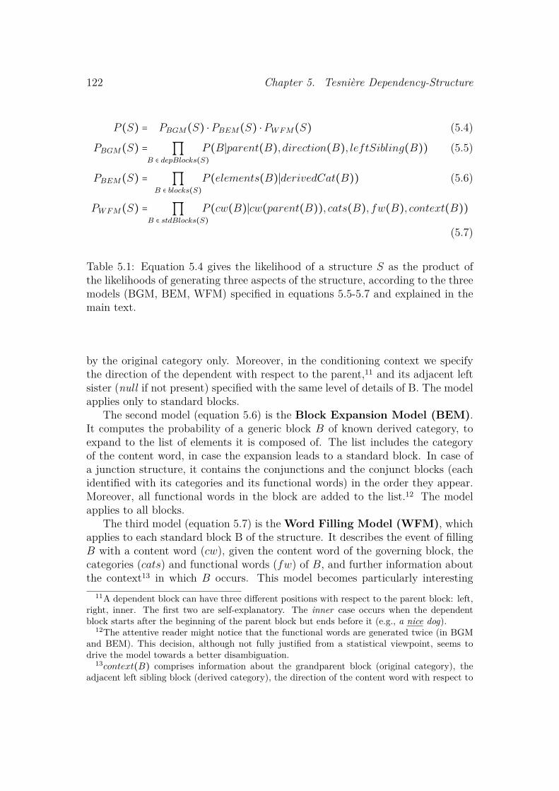
122 Chapter 5. Tesniere Dependency-Structure
P (S) = PBGM(S) ⋅ PBEM(S) ⋅ PWFM(S) (5.4)
PBGM(S) = ∏B ∈ depBlocks(S)
P (B∣parent(B), direction(B), leftSibling(B)) (5.5)
PBEM(S) = ∏B ∈ blocks(S)
P (elements(B)∣derivedCat(B)) (5.6)
PWFM(S) = ∏B ∈ stdBlocks(S)
P (cw(B)∣cw(parent(B)), cats(B), fw(B), context(B))
(5.7)
Table 5.1: Equation 5.4 gives the likelihood of a structure S as the product ofthe likelihoods of generating three aspects of the structure, according to the threemodels (BGM, BEM, WFM) specified in equations 5.5-5.7 and explained in themain text.
by the original category only. Moreover, in the conditioning context we specifythe direction of the dependent with respect to the parent,11 and its adjacent leftsister (null if not present) specified with the same level of details of B. The modelapplies only to standard blocks.
The second model (equation 5.6) is the Block Expansion Model (BEM).It computes the probability of a generic block B of known derived category, toexpand to the list of elements it is composed of. The list includes the categoryof the content word, in case the expansion leads to a standard block. In case ofa junction structure, it contains the conjunctions and the conjunct blocks (eachidentified with its categories and its functional words) in the order they appear.Moreover, all functional words in the block are added to the list.12 The modelapplies to all blocks.
The third model (equation 5.7) is the Word Filling Model (WFM), whichapplies to each standard block B of the structure. It describes the event of fillingB with a content word (cw), given the content word of the governing block, thecategories (cats) and functional words (fw) of B, and further information aboutthe context13 in which B occurs. This model becomes particularly interesting
11A dependent block can have three different positions with respect to the parent block: left,right, inner. The first two are self-explanatory. The inner case occurs when the dependentblock starts after the beginning of the parent block but ends before it (e.g., a nice dog).
12The attentive reader might notice that the functional words are generated twice (in BGMand BEM). This decision, although not fully justified from a statistical viewpoint, seems todrive the model towards a better disambiguation.
13context(B) comprises information about the grandparent block (original category), theadjacent left sibling block (derived category), the direction of the content word with respect to

5.5. A probabilistic Model for TDS 123
when a standard block is a dependent of a junction block (such as ‘abortion’ inFigure 5.9). In this case, the model needs to capture the dependency relationbetween the content word of the dependent block and each of the content wordsbelonging to the junction block.14
The conditional probabilities of the three models are smoothed using deletedinterpolation as in the models for DS (see §4.6.3). More details are provided inAppendix C.3.
PoS & Block tagging None of the previous 3 models take into account thelinear order of the words for deciding the locations of the block boundaries withina sentence. In order to improve robustness, we define 2 additional models forcomputing the probability of a given sequence of PoS-tags15 and block-tags forthe sequence of words of a given TDS structure. Both models are implementedas a tagging task with n-gram models as in chunking (Buchholz et al., 1999;Daelemans et al., 1999) and are shown in equations 5.8 and 5.9. In our casethe possible block-tags are: N (new block independent from the previous block),I (continue the previous block), -N (new block inside the previous block), C(coordination word), and +I (continue the parent block of the previous block).An example of a pos-tagging and block-tagging is illustrated in figure 5.6.
PPoS-tags(S) =n
∏i=1P (word(i), pos(i)∣wordi−1, posi−1, posi−2) (5.8)
PBlock-tags(S) =n
∏i=1P (block-tag(i)∣wordi, posi, posi−1, posi−2, posi+1) (5.9)
5.5.2 Experimental SetupWe have tested our model on the WSJ section of Penn Treebank Marcus et al.(1993), using sections 2-21 as training and section 22 for testing. We employthe Max-Ent parser implemented by Charniak (1999), to generate a list of k-best PS candidates for the test sentences, which are then converted into TDSrepresentation.
Instead of using Charniak’s parser in its original settings, we train it on aversion of the corpus in which we add a special suffix to constituents which havecircumstantial role.16 This decision is based on the observation that the TDSits governor (in this case only left and right), and the absolute distance between the two words.
14In order to derive the probability of this multi-event we compute the average between theprobabilities of the single events which compose it.
15Although PoS-tags are not represented in the graphical version of TDS trees, they are keptin the internal representation from the original PS.
16Those which have certain function tags (e.g., ADV, LOC, TMP). The full list is reportedin the post-processing procedure in §5.4.2. We were surprised to notice that the performance

124 Chapter 5. Tesniere Dependency-Structure
Mary
is singing
an
old and beautiful
song
N
N
V
VN
N
J
J
J
J
J
J
Words Mary is singing an old and beautiful songPoS-tags NNP VBZ VBG DT JJ CC JJ NNBlock-tags N N I N -N C N +I
Figure 5.6: Above: example of a TDS structure. Below: PoS-tags and block-tags associated to each word in the structure.
formalism captures the argument structure of verbs well, and we believe that thisadditional information might benefit our model.
We then applied our probabilistic model to re-rank the list of available k-bestTDS, and evaluate the selected candidates using several metrics which will beintroduced next.
5.5.3 Evaluation Metrics for TDSThe reranking framework described above, allows us to keep track of the originalPS of each TDS candidate. This provides an implicit advantage for evaluatingour system, viz. it allows us to evaluate the re-ranked structures both in termsof the standard evaluation benchmark on the original PS (F-score) as well as onmore refined metrics derived from the converted TDS representation. In addition,the specific head assignment that the TDS conversion procedure performs on theoriginal PS, allows us to convert every PS candidate to a standard projective DS,and from this representation we can in turn compute the benchmark evaluationfor DS used in §4.6.1, i.e., the unlabeled attachment score (UAS).
Concerning the TDS representation, we have formulated 3 evaluation metricswhich reflect the accuracy of the chosen structure with respect to the gold struc-ture (the one derived from the manually annotated PS), regarding the differentcomponents of the representation:
(in terms of F-score) of the parser on this modified treebank is only slightly lower than the oneobtained with standard settings (0.13%).
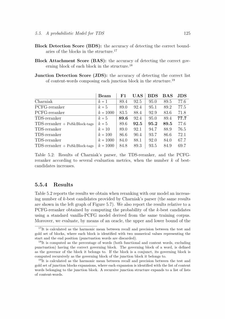
5.5. A probabilistic Model for TDS 125
Block Detection Score (BDS): the accuracy of detecting the correct bound-aries of the blocks in the structure.17
Block Attachment Score (BAS): the accuracy of detecting the correct gov-erning block of each block in the structure.18
Junction Detection Score (JDS): the accuracy of detecting the correct listof content-words composing each junction block in the structure.19
Beam F1 UAS BDS BAS JDSCharniak k = 1 89.4 92.5 95.0 89.5 77.6PCFG-reranker k = 5 89.0 92.4 95.1 89.2 77.5PCFG-reranker k = 1000 83.5 88.4 92.9 83.6 71.8TDS-reranker k = 5 89.6 92.4 95.0 89.4 77.7TDS-reranker + PoS&Block-tags k = 5 89.6 92.5 95.2 89.5 77.6TDS-reranker k = 10 89.0 92.1 94.7 88.9 76.5TDS-reranker k = 100 86.6 90.4 93.7 86.6 72.1TDS-reranker k = 1000 84.0 88.1 92.0 84.0 67.7TDS-reranker + PoS&Block-tags k = 1000 84.8 89.3 93.5 84.9 69.7
Table 5.2: Results of Charniak’s parser, the TDS-reranker, and the PCFG-reranker according to several evaluation metrics, when the number k of best-candidates increases.
5.5.4 ResultsTable 5.2 reports the results we obtain when reranking with our model an increas-ing number of k-best candidates provided by Charniak’s parser (the same resultsare shown in the left graph of Figure 5.7). We also report the results relative to aPCFG-reranker obtained by computing the probability of the k-best candidatesusing a standard vanilla-PCFG model derived from the same training corpus.Moreover, we evaluate, by means of an oracle, the upper and lower bound of the
17It is calculated as the harmonic mean between recall and precision between the test andgold set of blocks, where each block is identified with two numerical values representing thestart and the end position (punctuation words are discarded).
18It is computed as the percentage of words (both functional and content words, excludingpunctuation) having the correct governing block. The governing block of a word, is definedas the governor of the block it belongs to. If the block is a conjunct, its governing block iscomputed recursively as the governing block of the junction block it belongs to.
19It is calculated as the harmonic mean between recall and precision between the test andgold set of junction blocks expansions, where each expansion is identified with the list of contentwords belonging to the junction block. A recursive junction structure expands to a list of listsof content-words.

126 Chapter 5. Tesniere Dependency-Structure
Figure 5.7: Left: results of the TDS-reranking model according to several eval-uation metrics as in Table 5.2. Right: comparison between the F-scores of theTDS-reranker and a standard PCFG-reranker (together with the lower and theupper bound), with the increase of the number of best candidates. Results referto the development section (22) of the WSJ.
F-Score and JDS metric, by selecting the structures which maximizes/minimizesthe results.
Our reranking model performs rather well for a limited number of candidatestructures. In particular, for k = 5, it is in par or slightly outperforms Charniak’smodel for all evaluation metrics. In general, we notice that our extended modelincluding PoS-tagging and Block-tagging is more robust than our basic model,especially when reranking an high number of candidates.
The right graph in Figure 5.7 compares the F-score performance of the TDS-reranker against the PCFG-reranker. Our system consistently outperforms thePCFG model on this metric, as well as for UAS, BDS, and BAS. Concerningthe JDS metric, as the number of k-best candidates increases, the PCFG modeloutperforms the TDS-reranker.
5.6 Other representations of the WSJ TreebankIn this section we illustrate other proposed representations of the Penn WSJtreebank. Some of these are obtained fully automatically, while others have madeused of human annotators. In order to compare them and clarify better thecontribution of each representation we will take into consideration an exampletree from the WSJ treebank illustrate in figure 5.8. The corresponding TDS treeis presented in figure 5.9.

5.6. Other representations of the WSJ Treebank 127
S
NP-SBJ
DT
The
NN
rule
ADVP
RB
also
VP
VBZ
prohibits
NP
NP
NN
funding
PP
IN
for
NP
NP
NNS
activities
SBAR
WHNP
WDT
that
S
VP
VBP
encourage
,
,
VBP
promote
CC
or
VBP
advocate
NP
NN
abortion
Figure 5.8: Example of a PS tree of the WSJ treebank (section 0, #977).
Sentence # 1
The rule also
prohibits
funding
for activities
that encourage , promote or advocate
abortion
N
N
A
A
V
VN
NJ
NJ
V
J
V
J
V
J
V
N
N
Figure 5.9: TDS tree converted from the PS tree in figure 5.8.

128 Chapter 5. Tesniere Dependency-Structure
5.6.1 Prague English dependency treebankThe Prague English Dependency Treebank (Cinkova et al., 2008, 2009), in shortPEDT, consists of a semi-automatic conversion of a subset of the WSJ treebankinto a dependency representation which follows the scheme of the Prague Depen-dency Treebank (Hajic et al., 2000). Every sentence has two annotation layers:the analytical layer which captures the dependency surface-syntax, and the tec-togrammatical annotation, which encodes semantic relations between the contentwords in the sentence (the relations between content and functional words areonly included in the analytical layer). While the former is very similar to stan-dard labeled dependency grammar, the latter constitutes the main contribution ofthe proposed representation. The tectogrammatical representation derives fromthe Functional Generative Description tradition (Sgall et al., 1986), and aims atcapturing the linguistic meaning of the sentence, with special focus on the commu-nication role of language; for instance it includes underspecified elements whichcan be reconstructed from the context (e.g., in I told you last night, the verb hasan hidden argument to indicate that something has been told.). This represen-tation explicitly represents the argument structure of the sentence, and has beenused to automatically extract the valency frames of English verbs (Semecky andCinkova, 2006).
Figure 5.10 shows the tectogrammatical representation20 of the PS tree infigure 5.8. As in the TDS representation functional words (i.e., The, for) arerepresented together with the content words they refer to (i.e., rule, activity).
PDT representation employs only dependency relations to connect words.21
As in standard labeled dependency treebanks, this creates some problem whendealing with complex coordination (involving multiple conjuncts and shared ar-guments). In the same figure, we can in fact notice that there is no explicitrelation between any of the verbs in the coordinated structure (i.e., encourage,promote, advocate) and their arguments (i.e., that, abortion). This relations canbe retrieved only indirectly from the labels (i.e., RSTR.member, ACT, PAT ).
5.6.2 Stanford Typed Dependency RepresentationThe Stanford typed dependency representation (De Marneffe et al., 2006; De Mar-neffe and Manning, 2008) was developed with the aim of providing a suitablerepresentation for relation extraction and language understanding tasks. Theconversion is based on a completely automatic procedure which is part of theStanford parser software.22 The procedure takes as input any Penn-style PS tree-
20The PDT 2.0 treebank (both analytical and tectogrammatical layers) and visualizationsoftware are publicly available at http://ufal.mff.cuni.cz/pdt2.0. Many thanks to JanStepanek for technical assistance.
21Apart from standard governor-dependent relations it also encode anaphoric relations asshown in the same figure between that and activity.
22http://nlp.stanford.edu/software/

5.6. Other representations of the WSJ Treebank 129EnglishT-wsj_0049-s57root
ruleACT
alsoRHEM
prohibitPRED
fundingPAT
activityBEN
thatACT
encourageRSTR member
promoteRSTR member
orCONJ
advocateRSTR member
abortionPAT
rule The also
prohibits . ''
funding
activities for
that.
encourage.
promote
or
.advocate abortion
File: wsj_0049.t.gz, tree 57 of 76
The rule also prohibits funding for activities that `` *T*-137 encourage, promote or advocate abortion. ''Nařízení rovněž zakazuje financování činností, které "podporují, propagují nebo obhajují potraty".
Figure 5.10: Tectogrammatical annotation of the PS tree in figure 5.8 accordingto the Prague English Dependency Treebank.
bank and can output dependency-structures in various formats, among which thebase format, and the collapsed format which are reported in figure 5.11. Theformer is very similar to standard labeled dependency-structures, while in thelatter most of the relations between the content words and the functional wordsare collapsed into the labels of the relations.23 For instance in figure 5.11 thepreposition for in founding for activities is collapsed and put into the label ofthe dependency relation between founding and activities. The collapsed repre-sentation in this respect is very similar to the PEDT; the two representationsmainly diverge in the choice of the label hierarchy: the PEDT is more orientedtowards argument structure relations, while the Stanford representation followsmore traditional grammatical relations.
This representation has the same limitation as other dependency formalisms(e.g., PEDT) when dealing with coordination structures. The only main differencewith respect to the PEDT, is that Stanford dependency-structures choose the firstconjunct as the governor of a coordination construction.
23Not all the relations are collapsed. For instance prepositions are collapsed, while determin-ers are not.

130 Chapter 5. Tesniere Dependency-Structure
detDTThe
nsubjNNrule
advmodRBalso
rootVBZ
prohibits
dobjNN
funding
prepINfor
pobjNNS
activities
nsubjWDTthat
rcmodVBP
encourage
punct,,
conjVBP
promote
ccCCor
conjVBP
advocate
dobjNN
abortion
detDTThe
nsubjNNrule
advmodRBalso
rootVBZ
prohibits
dobjNN
funding
prep_forNNS
activities
rcmodVBP
encourage
conj_orVBP
promote
conj_orVBP
advocate
dobjNN
abortion
nsubjWDTthat
Figure 5.11: Stanford Dependency representation of part of the PS tree in fig-ure 5.8, in basic format (above) and collapsed format (below).

5.6. Other representations of the WSJ Treebank 131
5.6.3 Bubble TreesKahane (1997) described a general transformation of PS trees enriched with headlabels to a novel representations called bubble trees. A bubble tree incorporatesinformation from the original PS tree as well as the dependency relations implicitin the head annotation. Differently from standard PS to DS transforms (§4.3.1),the formalism allows to select more than a single daughter as head of a constituent.Figure 5.12 shows part of the bubble tree derived from PS tree in figure 5.8. Inthis representation every constituent is represented as a bubble (rectangles inthe figure). If constituent D is the head daughter of constituent P, D is placedinside P as a sub-bubble; otherwise it is a dependent of P (indicated with anarrow going from D to P). Therefore, as in the TDS representation, dependencyrelations are not between words but between bubbles (blocks in TDS). If multipledaughters are co-heads of the same constituent P, they are all placed inside P assub-bubbles. This allows to represent conjuncts of a coordination as sister nodeof the same bubble, as originally proposed by Tesniere. For instance in figure 5.12the three VBP of the rightmost VP are co-heads and positioned as daughters ofthe VP bubble.24 The use of both constituency relation and dependency relation,and the handling of coordination makes this formalism particularly similar to theTDS framework we have proposed. Although this transformation is insightful yetsimple to derive, it was unfortunately never applied to any treebank, nor used forbuilding parsing models.
5.6.4 The CCG-bankHockenmaier and Steedman (2007) developed a semi-automatic conversion of theWSJ treebank into Combinatory Categorial Grammar representation: the CCG-bank. CCG was introduced by Steedman (1996) as a generalization of Catego-rial Grammar theory (Ajdukiewicz, 1935; Bar-Hillel, 1953). It is a lexicalizedgrammar formalism, which can successfully represent a vast range of linguisticphenomena such as coordination, non local dependencies, control and raisingconstructions, without the use of movements and traces. Figure 5.13 representspart of the CCG-bank tree of the PS in figure 5.8. Internal constituents are as-signed either basic categories (e.g., S, NP), or complex categories (e.g., S/NP,NP/NP, (NP/NP)/NP)). In general, a complex category of the form X/Y expectsan argument Y to its right to produce a constituent of category X (forward com-position), while those of type X/Y expect Y to their left to produce X (backwardcomposition). For instance in the example tree of figure 5.13, NP/NP indicates aprepositional phrase which combined with an NP to its left produces an NP. For-ward/backward composition are somewhat similar to the transference operation
24The same formalism allows to represent blocks of words and transference as in TDS(see §5.2.4) by assigning heads to both the functional part and the content part of a constituent(e.g., in the same figure, WHNP and S can be co-heads of SBAR).
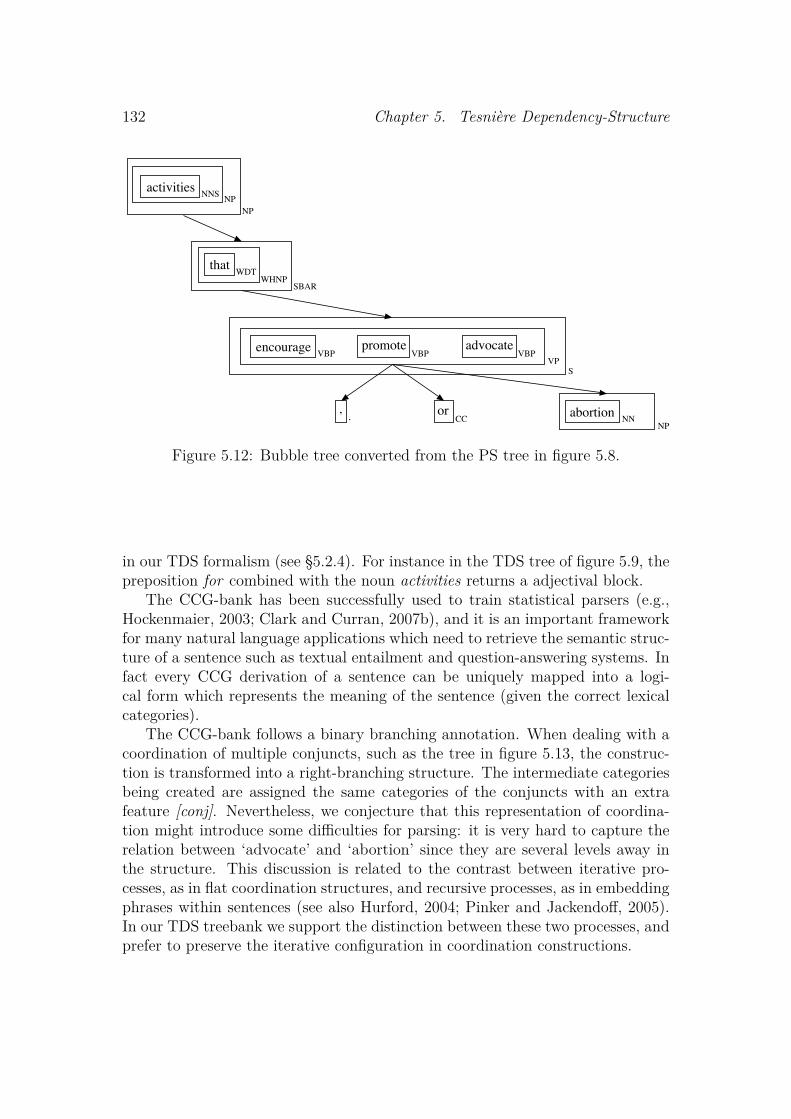
132 Chapter 5. Tesniere Dependency-Structure
activities
that
encourage
,
promote
or
advocate
abortion
NNS NPNP
NNNP
VBPVBPVBP
CC,
WDTWHNP
SBAR
VPS
Figure 5.12: Bubble tree converted from the PS tree in figure 5.8.
in our TDS formalism (see §5.2.4). For instance in the TDS tree of figure 5.9, thepreposition for combined with the noun activities returns a adjectival block.
The CCG-bank has been successfully used to train statistical parsers (e.g.,Hockenmaier, 2003; Clark and Curran, 2007b), and it is an important frameworkfor many natural language applications which need to retrieve the semantic struc-ture of a sentence such as textual entailment and question-answering systems. Infact every CCG derivation of a sentence can be uniquely mapped into a logi-cal form which represents the meaning of the sentence (given the correct lexicalcategories).
The CCG-bank follows a binary branching annotation. When dealing with acoordination of multiple conjuncts, such as the tree in figure 5.13, the construc-tion is transformed into a right-branching structure. The intermediate categoriesbeing created are assigned the same categories of the conjuncts with an extrafeature [conj]. Nevertheless, we conjecture that this representation of coordina-tion might introduce some difficulties for parsing: it is very hard to capture therelation between ‘advocate’ and ‘abortion’ since they are several levels away inthe structure. This discussion is related to the contrast between iterative pro-cesses, as in flat coordination structures, and recursive processes, as in embeddingphrases within sentences (see also Hurford, 2004; Pinker and Jackendoff, 2005).In our TDS treebank we support the distinction between these two processes, andprefer to preserve the iterative configuration in coordination constructions.

5.7. Assessment of the converted treebank 133
NP
NP
N
funding
NP/NP
(NP/NP)/NP
for
NP
NP
N
activities
NP/NP
(NP/NP)/(S/NP)
that
S/NP
(S/NP)/NP
(S/NP)/NP
encourage
(S/NP)/NP[conj]
,
,
(S/NP)/NP
(S/NP)/NP
promote
(S/NP)/NP[conj]
conj
or
(S/NP)/NP
advocate
NP
N
abortion
Figure 5.13: CCG representation of part of the PS tree in figure 5.8.
5.7 Assessment of the converted treebankFor a given syntactic representation it is always important to assess how well it isable to represent a specific linguistic phenomenon in theory and in practice. So farwe have described how both the TDS treebank and the CCG-bank are based ontheoretical formalisms which have one of the main strengths in the representationof coordination constructions. In order to complete our analysis, we report onan empirical study which compares the detection of coordination constructionsbetween the two treebanks.
The automatic detection of coordination in the WSJ treebank is not an easytask: for instance when conjuncts and modifiers of the coordination are put atthe same level (such as in the PS tree in figure 5.8), arguments can be wronglyidentified as conjuncts. In order to compare the quality of the CCG and TDStreebank for what concerns the identification of coordination structures, we haveidentified all the coordination construction in section 0 of the WSJ treebank forwhich the TDS and CCG analyses where not agreeing in the detection of co-ordination (168 sentences). With the help of an external annotator25 we havemanually annotated the correct coordination structures of those sentence anddetected the mistakes present in the two representations. As a quantitative sum-
25We are very grateful to Barend Beekhuizen for his help on annotating coordination con-structions.

134 Chapter 5. Tesniere Dependency-Structure
mary of this comparison, CCG presents 135 coordination mistakes,26 TDS only29, and there are 48 additional cases which are uncertain; more details of thiscomparison are illustrated in §C.2, while some examples of coordinated structuresin TDS representation are reported in Appendix C.4.
5.8 ConclusionIn this chapter we have formalized a novel syntactic scheme (TDS) inspired bythe work of Tesniere (1959), and developed a conversion algorithm to transformthe Penn Wall Street Journal treebank into the new representation.
Corpus-based computational linguistics has often valued a good compromisebetween adequacy and simplicity in the choice of linguistic representation. Thetransition from PS to DS notation has been seen as a useful simplification, butmany people have argued against its adequacy in representing frequent linguisticphenomena such as coordination. The TDS conversion presented in this chapter,reintroduces several key features from Tesniere’s work: on one hand the operationof junction enriches the model with a more adequate system to handle conjoinedstructures (e.g., coordination); on the other hand, the blocks, the transferenceoperation, and the category system further simplify and generalize the model.
We have presented a probabilistic generative model for parsing TDS syntacticrepresentation of English sentences. For evaluating the parsing performance wehave defined 3 metrics focusing on the different layers of the TDS representation(blocks, dependencies, coordinations). In particular we have introduced a specificmetric for the detection of coordination construction, a linguistic phenomenonhighly abundant in natural languages, but often neglected when it comes to eval-uating parsing resources, and hope that other researchers might benefit from itin the future. Our parsing results are encouraging: the overall system, althoughonly when the candidates are highly reliable, is in par or slightly improves onCharniak’s parser on all the evaluation metrics.
Finally we have compared the TDS treebank with other existing conversionsof the WSJ treebank, and assessed the quality of the conversion procedure withrespect to the detection of coordination constructions.
5.9 Future directionsGiven the availability of different syntactic representations for the sentences inthe WSJ treebank, one could follow the same manual assessment procedure wehave done for the detection of coordinating construction (see §5.7), while focusingon other shared linguistic phenomena (as in Rimell et al., 2009). The effort ofcomparing independently annotated resources is a stimulating task which brings
26In many case the CCG-bank misses the extra feature [conj].

5.9. Future directions 135
many insights in the investigated phenomena and leads to the corrections of manymistakes that occur in automatic as well as manual treebank annotations.
Moreover, as there exist a range of different syntactic representations thatavailable parsers are able to work with, it would be ideal to derive more univer-sally accepted evaluation criteria which could work across different representa-tions. Several attempts have been made in the past (Clark and Curran, 2007a;Rimell et al., 2009), but they are not widely employed as they require substantialannotation effort. An easier alternative for comparing different representationson the same metrics, is to rely on transformation techniques. For instance, theavailability of an automatic conversion from Penn-style PS trees to TDS repre-sentation, could allow us to test the performance of a range of state-of-the-art PSparsers on the more refined evaluation criteria we have introduced for the TDSrepresentation, and in particular on the detection of coordination constructions.


It was six men of IndostanTo learning much inclined,Who went to see the Elephant(Though all of them were blind),That each by observationMight satisfy his mind.The First approached the Elephant,And happening to fallAgainst his broad and sturdy side,At once began to bawl:”God bless me!-but the ElephantIs very like a wall!”The Second, feeling of the tusk,Cried: ”Ho!-what have we hereSo very round and smooth and sharp?To me’t is mighty clearThis wonder of an ElephantIs very like a spear!”The Third approached the animal,And happening to takeThe squirming trunk within his hands,Thus boldly up and spake:”I see,” quoth he, ”the ElephantIs very like a snake!”[...]And so these men of IndostanDisputed loud and long,Each in his own opinionExceeding stiff and strong,Though each was partly in the right,And all were in the wrong!
John Godfrey Saxe
Chapter 6Conclusions
137

138 Chapter 6. Conclusions
At the beginning of this thesis we have stressed how current computationallinguistic research seems to be drifting away from linguistic theory. One of themain motivations behind our work was therefore to contribute to reversing thistendency, by investigating several computational models of syntax while keepingin mind the original linguistic view on the studied phenomena.
One of the main points of divergence between the two fields is the difficulty totranslate a number of syntactic models over various tree structure representationsinto computational models that can be learned and tested empirically. In chapter2 we have therefore presented a general methodology for simplifying the task offormalizing theory-independent probabilistic generative models for various treestructures. One of the main objectives behind this work was to stimulate morediversification in computational linguistics concerning the syntactic representa-tion underlying the models and the linguistic theories for generating them. Theproposed methodology is in fact able to generalize over a number of tree-basedtheories by providing i) a unique description of the sequence of events charac-terizing the generation of the syntactic analyses of a given sentence according tovarious models, and ii) a way to map a symbolic grammar into a probabilisticmodel.
We have applied this methodology to three distinct syntactic representa-tions: simple phrase-structure (PS), dependency-structure (DS), and Tesnieredependency-structure (TDS). After comparing PS and DS on theoretical grounds,we have shown how they can be seen as two complementary representations forsyntax. We have therefore formalized TDS as an intermediate representation be-tween PS and DS which is better at representing linguistic phenomena such ascoordination. We have experimented on the three schemes empirically, throughthe implementation of computational models for generating syntactic analysesaccording to the three representations.
For phrase-structure trees, in chapter 3 we have proposed a novel Data-Oriented Parsing formalism (Double-DOP) based on an explicit representationof arbitrarily large syntactic fragments. As the number of all possible construc-tions which can be extracted from a large treebank is extremely large, we need toresort to a restricted yet representative subset of fragments. We therefore proposea linguistically motivated methodology to automatically identify those fragmentsfor which there is evidence about their reusability. We achieved this by means ofa special-purpose application (Fragment-Seeker), based on an efficient tree-kernelalgorithm.
Both Fragment-Seeker and the Double-DOP parser are made available to thelinguistic community at large, and we hope they will prove useful in linguisticresearch as well as other NLP applications. In particular, as the identificationof syntactic constructions has always represented one of the biggest challengesin linguistic theory (Fillmore et al., 1988; Goldberg, 1995; Kay and Fillmore,1997), we believe that further investigation into reusable fragments could provide

139
fruitful insights for studying linguistic phenomena pertaining to the identificationof syntactic constructions such as subcategorization, idiomatic expressions, andmultiword expressions. Regarding NLP applications, we expect that Fragment-Seeker and Double-DOP could be used as a component for competitive systemsfor solving linguistic tasks such as machine translation, semantic role labeling,question-answering and speech recognition systems.
For DS trees, in chapter 4 we have compared a number of probabilistic gen-erative bilexical models initially proposed by Eisner (1996a,b) and experimentedwith some of their variations. Although the different models greatly differ in theirlinguistic hypotheses on the types of rules and features that are considered in therespective grammars, we were able to efficiently compare them by resorting to thegeneralized representation of the event space as presented in chapter 2, and byrelying on a reranking methodology. Reranking can be seen as a useful approachfor easily evaluating a number of generative models of syntax and approximatingthe behavior of a full-fledged probabilistic parser which would need to be specif-ically implemented and optimized for the chosen model. In our implementation,in fact, the reranking approach can be seen as a parser simulator which mimicall the choices a model would perform to obtain a certain analysis of a givensentence. This approach could also be employed as a linguistic tool to better un-derstand why, under a specific probabilistic model, certain analyses are preferredover others.
Looking at the last 100 years or so, one of the main aspects of linguisticresearch has been the search for more adequate syntactic representations. Incontrast, in computational linguistics, the difficulty of building large manuallyannotated treebanks has often represented a major obstacle for empirically inves-tigating a wide range of syntactic representations. In chapter 5 we contributedto bridging this gap, by introducing a novel syntactic scheme based on the for-malization of the original work on dependency syntax of Lucien Tesniere (1959),and therefore called Tesniere Dependency-Structure (TDS). In our opinion, thisconstitutes a very promising formalism for linguistic representation although onlysome aspects of it have been used in computational linguistics: modern DS re-tains only the main idea proposed by Tesniere, namely the relation of dependencybetween words, while other operations and features of the original theory are dis-carded or not overtly represented. More specifically, TDS can be seen as anintermediate representation between phrase-structure and dependency-structure,as it uses constituencies to groups adjacent words (chunks) and to represent co-ordination constructions, while it adopts dependency relations to link togetherthe syntactic units (chunks and coordination constructions).
In order to investigate such a representation empirically, we have implementedan automatic procedure for converting the English WSJ treebank into TDS nota-tion, and used the converted treebank to test a new computational, probabilistic

140 Chapter 6. Conclusions
model for generating TDS analyses of novel sentences. This model was imple-mented using a reranking framework similar to the one used for testing DS models.
Finally, in order to evaluate this model we have defined three separate metricsspecific to the linguistic features represented in TDS, namely, chunks, dependen-cies, and coordination. As currently used evaluation metrics for parsing haveoften raised skepticism about the extent by which they are able to quantify thecorrectness of the derived analyses, we hope that our attempt to define a rangeof linguistically motivated evaluation metrics may be useful for the parsing com-munity.
After the statistical revolution of the ’90s in computational linguistics, most ofthe computational models of syntax have been focusing on phrase-structure andonly more recently on dependency-structure. Deep syntactic representations (e.g.,HPSG, LFG) have had more marginal roles in the parsing community because ofthe lack of significant annotated resources and the difficulty of deriving efficientmodels. By proposing a novel TDS scheme we have attempted to push forwardthe requirements probabilistic parsers should meet, by compromising betweenlinguistically adequate representations and efficient generative models for parsing.

Appendix APhrase-Structure Models
A.1 Models parametersIn table A.1 we report the parameters used to obtain the parsing results in ta-ble 3.3. These were chosen in order to maximize results on the developmentsection of the corresponding treebank (for parsing the Brown corpus, for whichthere is no standard development section, we have used the same parameters usedfor the WSJ). All models use the same binarization (see §3.7) with H=1, P=1.
Unknown Threshold words occurring less than this threshold are substitutewith word-features.
Unknown Word Model the 5 different models as in Berkeley code to specifyhow unknown words are converted into word-features (5 is the most specificto English, 1 is the most generic).
σ Open-class threshold used for smoothing (see §3.7). A PoS-tag is an open classif it rewrites to at least σ different words in the training corpus. A word isan open class word if it has been seen only with open-class PoS-tags.
ε Low frequency count assigned to open-class ⟨ word, PoS-tag ⟩ pairs not encoun-tered in the training corpus.
λ Threshold to maximize F1 score, as illustrated in §3.6.3.
141

142 Appendix A. Phrase-Structure Models
Treebank Parsing Model UnknownThreshold
UnknownWordModel
σ ε λ
WSJ PCFG 4 1 50 0.01 -Double-DOP 4 5 50 0.01 1.10
Brown PCFG 1 1 50 0.01 -Double-DOP 1 5 50 0.01 1.10
Negra PCFG 9 4 50 0.01 -Double-DOP 9 4 50 0.01 0.95
FTB PCFG 1 4 50 0.01 -Double-DOP 1 4 50 0.01 1.45
CTB 3.0 PCFG 1 4 50 0.01 -Double-DOP 1 4 50 0.01 1.05
HTB PCFG 1 1 100 0.01 -Double-DOP 1 1 100 0.01 1.05
Table A.1: Parameters used to obtained the results in table 3.3.
A.2 Evaluation procedureEvalB discards traces (and semantic tags) but does not remove redundant rulesthat result from the elimination of traces (and semantic tags). See for instancethe example structure in figure A.1. For obtaining the cleaned version of the filei apply the following steps:
• prune traces subtrees (-NONE-)
• remove numbers in labels (e.g., NP-2 or NP=2)
• remove semantic tags (e.g., NP-SBJ)
• remove redundant rules (e.g., NP Ð→ NP)

A.2. Evaluation procedure 143
S-2
NP-SBJ
NP
PRP
It
S
-NONE-
*EXP*-1
VP
VBZ
is
ADJP-PRD
JJ
easy
S-1
NP-SBJ
-NONE-
*
VP
TO
to
VP
VB
say
SBAR
-NONE-
0
S
NP-SBJ
DT
the
NN
specialist
VP
VBZ
is
RB
n’t
VP
VBG
doing
NP
PRP$
his
NN
jobS
NP
PRP
It
VP
VBZ
is
ADJP
JJ
easy
S
VP
TO
to
VP
VB
say
SBAR
S
NP
DT
the
NN
specialist
VP
VBZ
is
RB
n’t
VP
VBG
doing
NP
PRP$
his
NN
job
Figure A.1: (sec 23, 11th structure)
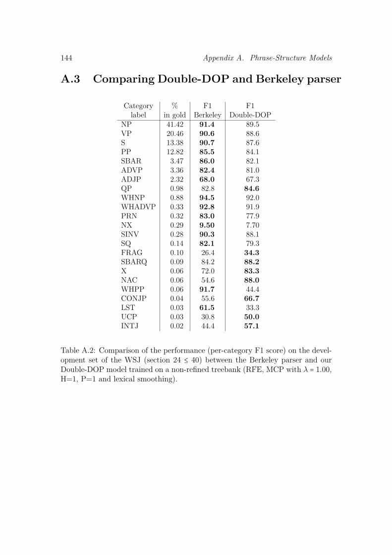
144 Appendix A. Phrase-Structure Models
A.3 Comparing Double-DOP and Berkeley parser
Category % F1 F1label in gold Berkeley Double-DOP
NP 41.42 91.4 89.5VP 20.46 90.6 88.6S 13.38 90.7 87.6PP 12.82 85.5 84.1SBAR 3.47 86.0 82.1ADVP 3.36 82.4 81.0ADJP 2.32 68.0 67.3QP 0.98 82.8 84.6WHNP 0.88 94.5 92.0WHADVP 0.33 92.8 91.9PRN 0.32 83.0 77.9NX 0.29 9.50 7.70SINV 0.28 90.3 88.1SQ 0.14 82.1 79.3FRAG 0.10 26.4 34.3SBARQ 0.09 84.2 88.2X 0.06 72.0 83.3NAC 0.06 54.6 88.0WHPP 0.06 91.7 44.4CONJP 0.04 55.6 66.7LST 0.03 61.5 33.3UCP 0.03 30.8 50.0INTJ 0.02 44.4 57.1
Table A.2: Comparison of the performance (per-category F1 score) on the devel-opment set of the WSJ (section 24 ≤ 40) between the Berkeley parser and ourDouble-DOP model trained on a non-refined treebank (RFE, MCP with λ = 1.00,H=1, P=1 and lexical smoothing).

Appendix BDependency-Structure Models
B.1 DS to PSThe way to transform DS into PS is less discussed in the literature. The procedureillustrated here is recursive, and takes into consideration a DS rooted in node w.Three general cases can be encountered:
1. w is a terminal node (it has no dependents): in this case the resulting PShas a single terminal node W .
2. w has a single dependent. The corresponding PS has two daughter nodes:the PS obtained by transforming the dependent, and a single-node PS con-taining the governing word w. The two daughters will keep the same linearorder as in the original DS.
3. w has k dependents d1, d2, . . . , dk (k > 1). In this last case w is mapped into asingle terminal PS node W , and each dependent dj is transformed into a PSDj (recursive step). Given that w occurs after the ith dependent we can rep-resent k+1 trees in a single sequence of nodes as D1, . . . ,Di,W,Di+1, . . . ,Dk.At this point, we need to choose how to group these k+1 nodes into a seriesof hierarchical PS trees P1, P2, . . . , Pm (1 ≤m ≤ k), such that:
- Pj must form a contiguous span (for every 1 ≤ j ≤m).- P1 must contain as daughter W and at least one other node.1 In order
to form a contiguous span this is either Di or Di+1 (e.g., D1,W,D3 isnot allowed).
- Pj+1 must contain Pj as daughter, together with at least another nodefrom the initial sequence D1, . . . ,Dk (for every 1 ≤ j < m). The set ofselected daughters should yield a contiguous span of the sentence.
1P1 could contain W alone if we allow unary chains.
145

146 Appendix B. Dependency-Structure Models
- Pm must contain directly (as daughter) or indirectly (daughters ofdaughters) all k + 1 nodes in the initial sequence.
The resulting PS is rooted in Pm.
Case 3 of this procedure is the only one which requires a choice to be made. Infact, as we can see in figure 4.3, DS trees A,B,F,G are mapped into a single PSbecause they do not contain any node with more than one dependent. Tree D,instead, has a node with 2 dependents. Following case 3, we have three choices:
1. (m = 1) group the governor (2) and all the dependents (1,3) in a uniqueconstituent, resulting in PS tree β;
2. (m = 2) group first the governor (2) with the left dependent (1) and theresulting constituent to the remaining dependent (3), resulting in PS treeγ;
3. (m = 2) group first the governor (2) with the right dependent (3) and theresulting constituent to the remaining dependent (1), resulting in PS treeα.
The general idea behind the study conducted by Hays (1960) is that PS andDS are complementary in nature. PS well represents constituents but leavesthe notion of heads underspecified, while DS is based on governing-dependencyrelations but does not specify how to group multiple dependents of the samegovernor.
Gaifman (1965) claims that a given DS has a “naturally corresponding” PS,such that every DS maps to a single PS, but not vice versa (a single PS may mapto multiple DS trees). This is a somehow misleading claim since it is based on anad-hoc definition of equivalence between PS and DS. According to this definition,given a DS there exists a unique equivalent PS tree obtained by imposing m = 1in the procedure above: the PS should contain the same number of constituentsas there are governors in the DS, and each constituent should expand to a set ofwords including the associated governor together with all the words that dependdirectly or indirectly from it. This mapping is illustrated in figure 4.3 with dashedlines. According to this mapping we still have some PS mapping to multiple DSs(remember that DSs are always more in number), but in this case we have morerestrictions than before: the head of each constituent must be chosen among thedaughter node of minimum depth, where the depth of a node is defined as thelength of the longest path connecting the node to one of the terminal node underits span.
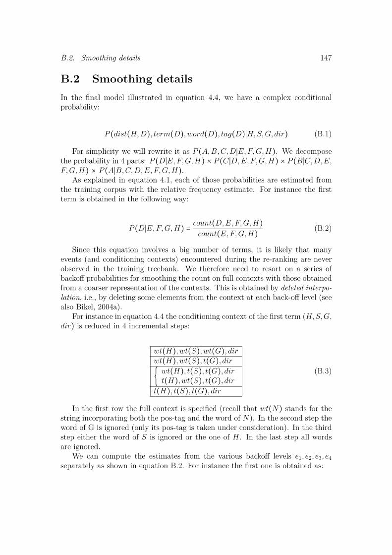
B.2. Smoothing details 147
B.2 Smoothing detailsIn the final model illustrated in equation 4.4, we have a complex conditionalprobability:
P (dist(H,D), term(D),word(D), tag(D)∣H,S,G, dir) (B.1)
For simplicity we will rewrite it as P (A,B,C,D∣E,F,G,H). We decomposethe probability in 4 parts: P (D∣E,F,G,H) × P (C ∣D,E,F,G,H) × P (B∣C,D,E,F,G,H) × P (A∣B,C,D,E,F,G,H).
As explained in equation 4.1, each of those probabilities are estimated fromthe training corpus with the relative frequency estimate. For instance the firstterm is obtained in the following way:
P (D∣E,F,G,H) = count(D,E,F,G,H)count(E,F,G,H) (B.2)
Since this equation involves a big number of terms, it is likely that manyevents (and conditioning contexts) encountered during the re-ranking are neverobserved in the training treebank. We therefore need to resort on a series ofbackoff probabilities for smoothing the count on full contexts with those obtainedfrom a coarser representation of the contexts. This is obtained by deleted interpo-lation, i.e., by deleting some elements from the context at each back-off level (seealso Bikel, 2004a).
For instance in equation 4.4 the conditioning context of the first term (H,S,G,dir) is reduced in 4 incremental steps:
wt(H),wt(S),wt(G), dirwt(H),wt(S), t(G), dir
{ wt(H), t(S), t(G), dirt(H),wt(S), t(G), dir
t(H), t(S), t(G), dir
(B.3)
In the first row the full context is specified (recall that wt(N) stands for thestring incorporating both the pos-tag and the word of N). In the second step theword of G is ignored (only its pos-tag is taken under consideration). In the thirdstep either the word of S is ignored or the one of H. In the last step all wordsare ignored.
We can compute the estimates from the various backoff levels e1, e2, e3, e4separately as shown in equation B.2. For instance the first one is obtained as:
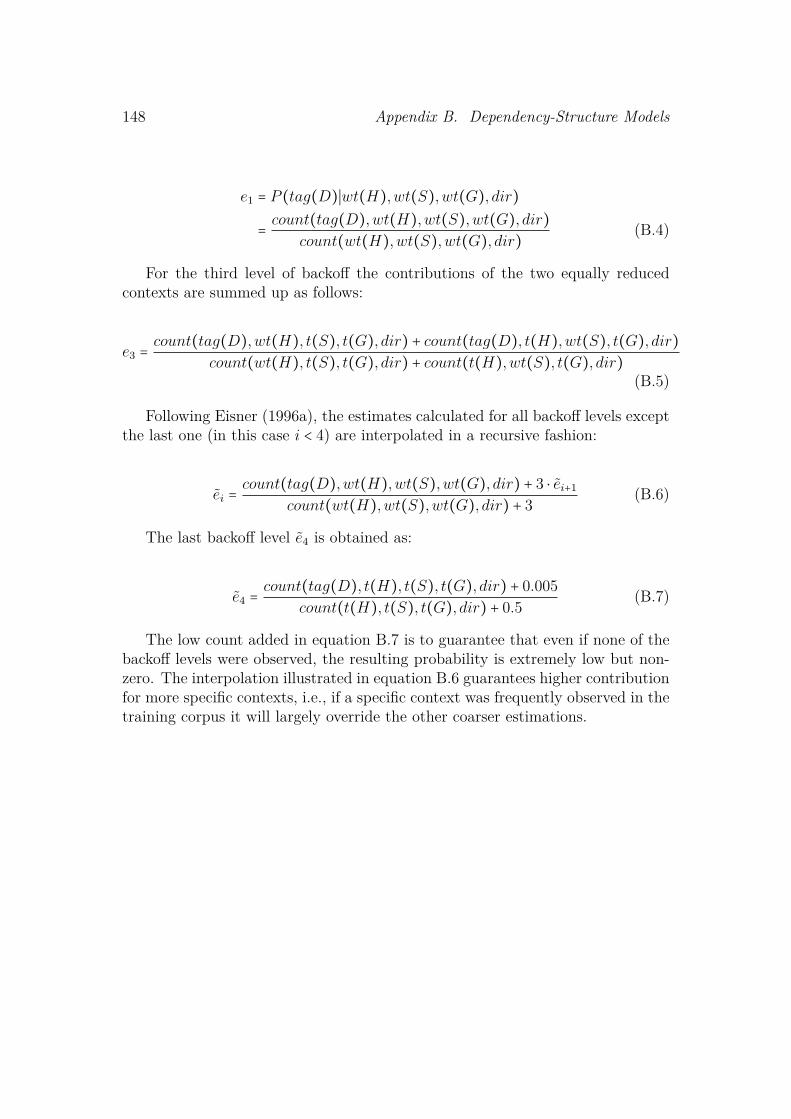
148 Appendix B. Dependency-Structure Models
e1 = P (tag(D)∣wt(H),wt(S),wt(G), dir)
= count(tag(D),wt(H),wt(S),wt(G), dir)count(wt(H),wt(S),wt(G), dir) (B.4)
For the third level of backoff the contributions of the two equally reducedcontexts are summed up as follows:
e3 =count(tag(D),wt(H), t(S), t(G), dir) + count(tag(D), t(H),wt(S), t(G), dir)
count(wt(H), t(S), t(G), dir) + count(t(H),wt(S), t(G), dir)(B.5)
Following Eisner (1996a), the estimates calculated for all backoff levels exceptthe last one (in this case i < 4) are interpolated in a recursive fashion:
ei =count(tag(D),wt(H),wt(S),wt(G), dir) + 3 ⋅ ei+1
count(wt(H),wt(S),wt(G), dir) + 3 (B.6)
The last backoff level e4 is obtained as:
e4 =count(tag(D), t(H), t(S), t(G), dir) + 0.005
count(t(H), t(S), t(G), dir) + 0.5 (B.7)
The low count added in equation B.7 is to guarantee that even if none of thebackoff levels were observed, the resulting probability is extremely low but non-zero. The interpolation illustrated in equation B.6 guarantees higher contributionfor more specific contexts, i.e., if a specific context was frequently observed in thetraining corpus it will largely override the other coarser estimations.

Appendix CTDS model
C.1 Head annotationWe report below the head annotation table used to perform the conversion ofthe Penn WSJ Treebank into TDS representation (see section 5.4.2). For a givenCFG rule in the treebank, the table describes which daughter node (in the righthand-side of the rule) is marked as head. Each parent node in the table (lefthand-side of the rule) is mapped to a list of sub-rules (rows in the table). Ifthe first sub-rule does not apply the second is considered, if not the third, andso on. In each sub-rule the daughter nodes in the rule are read according tothe specified start direction in the second column (left/right). The third columnrefers to the priority: if it is set to D (daughters), all daughters are checkedagainst the first element in the list, if none applies, against the second elementthe list, the third, and so on; if it is set to L (list) all elements in the list (fromleft to right) are checked against the first daughter, if it does not match, againstthe second daughter, the third, and so on. The special symbol * matches anylabel, and is inserted at the end of the last sub-rule to ensure that there is alwaysan head-daughter for each rule.
Parent Start Priority ListADJP left D NNS, QP, NN, NML, $
right D JJleft D ADVP, VBN, VBG, AUX, AUXG, ADJP,
JJR, JJS, JJP, FW, RBR, RBS, RB, NP,SBAR, DT, *
ADVP right D RB, RBR, RBS, FW, ADVP, CD, JJR, JJ,JJP, NP, NML, JJS, NN, TO, IN, *
CONJP right D RB, IN, *FRAG left D NP, NML, VP, ADJP, PP, *
149

150 Appendix C. TDS model
INTJ left D *LST right D LS, :, *NAC left L NN, NNS, NNP, NNPS, NP, NAC, NML,
EX, $, CD, QP, PRP, VBG, AUX, AUXG,JJ, JJS, JJR, JJP, ADJP, FW, *
NP right L NN, NNS, NX, NNP, NNPS, NMLleft L NP
right L $ ADJP, PRNright L CDright L JJR, JJ, JJS, JJP, RB, QPright D *
NML right L NN, NNP, NNPS, NNS, NX, NML, JJRleft L NP
right L $, ADJP, PRNright L CDright L JJ, JJS, JJP, RB, QPright D *
NX right D NP, NXright L NNPS, NNS, NNP, NN, NML, JJR, JJP, *
JJP right L JJ, JJR, JJS, JJP, VBG, *PP right D VBG, VBN, AUX, AUXG, RP, FW, NP,
SBAR, S, IN, TO, *PRN left D VP, NP, PP, *PRT right D RP, *QP left D $, NNS, NN, NML, JJ, RB, CD, NCD, QP,
JJR, JJS, JJP, IN, DT, *RRC right D VP, NP, ADVP, ADJP, PP, *
S left D VP, S, SBAR, ADJP, UCP, NP, TO, IN, *SBAR left D NN, NML
left D S, SQ, SINV, SBAR, FRAG, WHNP,WHPP, WHADVP, WHADJP, IN, DT, *
SBARQ left D SQ, S, SINV, SBARQ, FRAG, *SINV left D VBZ, VBD, VBP, VB, AUX, AUXG, VP, S,
SINV, ADJP, NP, NML, MD, *SQ left D VBZ, VBD, VBP, VB, AUX, AUXG, VP,
SQ, MD, *UCP right D *VP left D VBD, VBN, VBZ, VB, VBG, VBP, AUX,
AUXG, VP, ADJP, NN, NNS, NP, NML,MD, TO, JJ, JJP, *
WHADJP left D WRB, JJ, JJP, ADJP, *
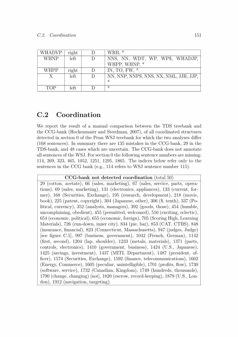
C.2. Coordination 151
WHADVP right D WRB, *WHNP left D NNS, NN, WDT, WP, WP$, WHADJP,
WHPP, WHNP, *WHPP right D IN, TO, FW, *
X left D NN, NNP, NNPS, NNS, NX, NML, JJR, JJP,*
TOP left D *
C.2 CoordinationWe report the result of a manual comparison between the TDS treebank andthe CCG-bank (Hockenmaier and Steedman, 2007), of all coordinated structuresdetected in section 0 of the Penn WSJ treebank for which the two analyses differ(168 sentences). In summary there are 135 mistakes in the CCG-bank, 29 in theTDS-bank, and 48 cases which are uncertain. The CCG-bank does not annotateall sentences of the WSJ. For section 0 the following sentence numbers are missing:114, 269, 323, 465, 1052, 1251, 1295, 1865. The indices below refer only to thesentences in the CCG bank (e.g., 114 refers to WSJ sentence number 115).
CCG-bank not detected coordination (total 50)29 (cotton, acetate), 66 (sales, marketing), 67 (sales, service, parts, opera-tions), 69 (sales, marketing), 131 (electronics, appliances), 133 (current, for-mer), 168 (Securities, Exchange), 195 (research, development), 218 (movie,book), 225 (patent, copyright), 304 (Japanese, other), 306 ($, tenth), 337 (Po-litical, currency), 352 (analysts, managers), 392 (goods, those), 454 (humble,uncomplaining, obedient), 455 (permitted, welcomed), 516 (exciting, eclectic),654 (economic, political), 655 (economic, foreign), 705 (Scoring High, LearningMaterials), 726 (run-down, inner city), 834 (pie, bar), 853 (CAT, CTBS), 848(insurance, financial), 823 (Connecticut, Massachusetts), 947 (judges, Judge)[see figure C.5], 997 (business, government), 1042 (French, German), 1142(first, second), 1204 (lap, shoulder), 1233 (metals, materials), 1371 (parts,controls, electronics), 1410 (government, business), 1424 (U.S., Japanese),1425 (savings, investment), 1437 (MITI, Department), 1487 (president, of-ficer), 1574 (Securities, Exchange), 1592 (finance, telecommunications), 1602(Energy, Commerce), 1605 (peculiar, unintelligible), 1701 (profits, flow), 1730(software, service), 1732 (Canadian, Kingdom), 1749 (hundreds, thousands),1790 (change, changing) [not], 1820 (escrow, record-keeping), 1879 (U.S., Lon-don), 1912 (navigation, targeting).
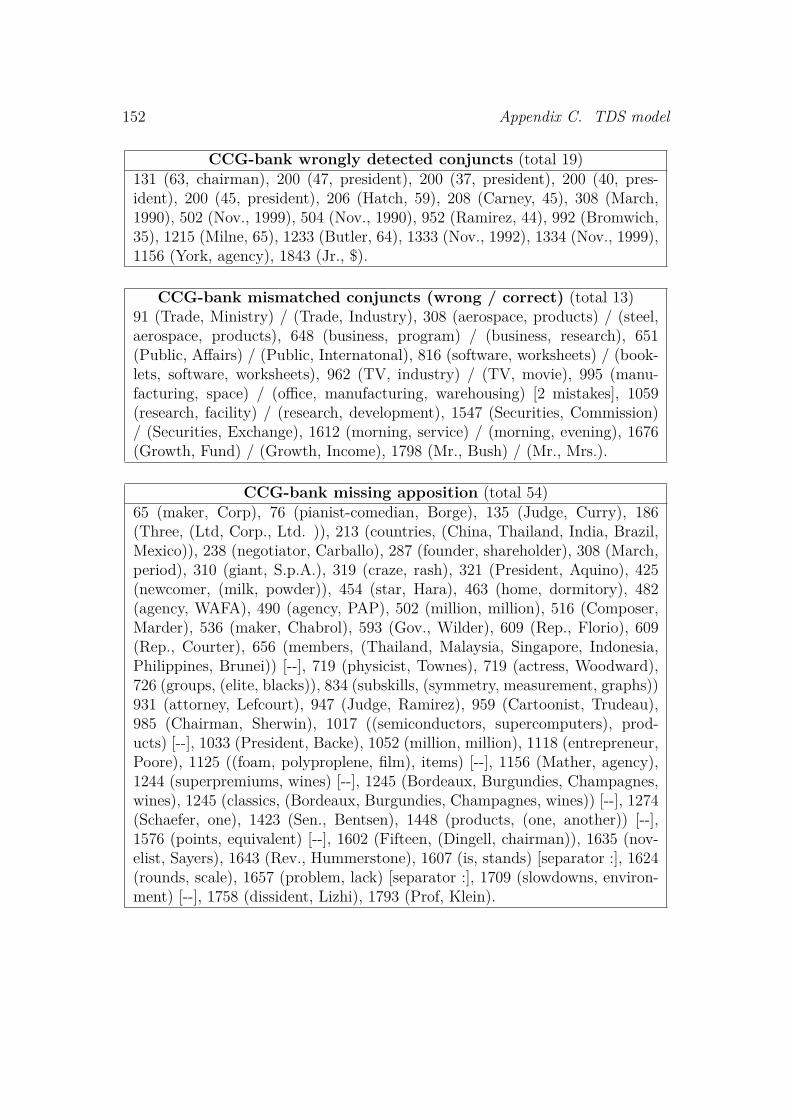
152 Appendix C. TDS model
CCG-bank wrongly detected conjuncts (total 19)131 (63, chairman), 200 (47, president), 200 (37, president), 200 (40, pres-ident), 200 (45, president), 206 (Hatch, 59), 208 (Carney, 45), 308 (March,1990), 502 (Nov., 1999), 504 (Nov., 1990), 952 (Ramirez, 44), 992 (Bromwich,35), 1215 (Milne, 65), 1233 (Butler, 64), 1333 (Nov., 1992), 1334 (Nov., 1999),1156 (York, agency), 1843 (Jr., $).
CCG-bank mismatched conjuncts (wrong / correct) (total 13)91 (Trade, Ministry) / (Trade, Industry), 308 (aerospace, products) / (steel,aerospace, products), 648 (business, program) / (business, research), 651(Public, Affairs) / (Public, Internatonal), 816 (software, worksheets) / (book-lets, software, worksheets), 962 (TV, industry) / (TV, movie), 995 (manu-facturing, space) / (office, manufacturing, warehousing) [2 mistakes], 1059(research, facility) / (research, development), 1547 (Securities, Commission)/ (Securities, Exchange), 1612 (morning, service) / (morning, evening), 1676(Growth, Fund) / (Growth, Income), 1798 (Mr., Bush) / (Mr., Mrs.).
CCG-bank missing apposition (total 54)65 (maker, Corp), 76 (pianist-comedian, Borge), 135 (Judge, Curry), 186(Three, (Ltd, Corp., Ltd. )), 213 (countries, (China, Thailand, India, Brazil,Mexico)), 238 (negotiator, Carballo), 287 (founder, shareholder), 308 (March,period), 310 (giant, S.p.A.), 319 (craze, rash), 321 (President, Aquino), 425(newcomer, (milk, powder)), 454 (star, Hara), 463 (home, dormitory), 482(agency, WAFA), 490 (agency, PAP), 502 (million, million), 516 (Composer,Marder), 536 (maker, Chabrol), 593 (Gov., Wilder), 609 (Rep., Florio), 609(Rep., Courter), 656 (members, (Thailand, Malaysia, Singapore, Indonesia,Philippines, Brunei)) [--], 719 (physicist, Townes), 719 (actress, Woodward),726 (groups, (elite, blacks)), 834 (subskills, (symmetry, measurement, graphs))931 (attorney, Lefcourt), 947 (Judge, Ramirez), 959 (Cartoonist, Trudeau),985 (Chairman, Sherwin), 1017 ((semiconductors, supercomputers), prod-ucts) [--], 1033 (President, Backe), 1052 (million, million), 1118 (entrepreneur,Poore), 1125 ((foam, polyproplene, film), items) [--], 1156 (Mather, agency),1244 (superpremiums, wines) [--], 1245 (Bordeaux, Burgundies, Champagnes,wines), 1245 (classics, (Bordeaux, Burgundies, Champagnes, wines)) [--], 1274(Schaefer, one), 1423 (Sen., Bentsen), 1448 (products, (one, another)) [--],1576 (points, equivalent) [--], 1602 (Fifteen, (Dingell, chairman)), 1635 (nov-elist, Sayers), 1643 (Rev., Hummerstone), 1607 (is, stands) [separator :], 1624(rounds, scale), 1657 (problem, lack) [separator :], 1709 (slowdowns, environ-ment) [--], 1758 (dissident, Lizhi), 1793 (Prof, Klein).
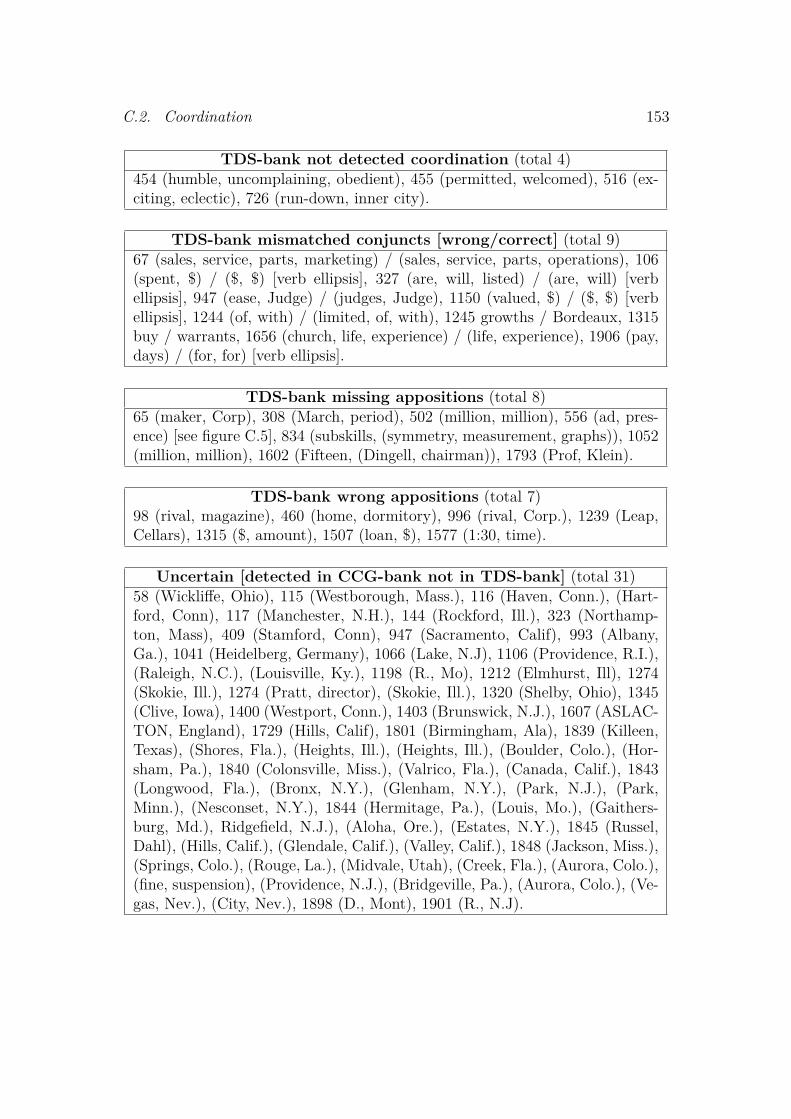
C.2. Coordination 153
TDS-bank not detected coordination (total 4)454 (humble, uncomplaining, obedient), 455 (permitted, welcomed), 516 (ex-citing, eclectic), 726 (run-down, inner city).
TDS-bank mismatched conjuncts [wrong/correct] (total 9)67 (sales, service, parts, marketing) / (sales, service, parts, operations), 106(spent, $) / ($, $) [verb ellipsis], 327 (are, will, listed) / (are, will) [verbellipsis], 947 (ease, Judge) / (judges, Judge), 1150 (valued, $) / ($, $) [verbellipsis], 1244 (of, with) / (limited, of, with), 1245 growths / Bordeaux, 1315buy / warrants, 1656 (church, life, experience) / (life, experience), 1906 (pay,days) / (for, for) [verb ellipsis].
TDS-bank missing appositions (total 8)65 (maker, Corp), 308 (March, period), 502 (million, million), 556 (ad, pres-ence) [see figure C.5], 834 (subskills, (symmetry, measurement, graphs)), 1052(million, million), 1602 (Fifteen, (Dingell, chairman)), 1793 (Prof, Klein).
TDS-bank wrong appositions (total 7)98 (rival, magazine), 460 (home, dormitory), 996 (rival, Corp.), 1239 (Leap,Cellars), 1315 ($, amount), 1507 (loan, $), 1577 (1:30, time).
Uncertain [detected in CCG-bank not in TDS-bank] (total 31)58 (Wickliffe, Ohio), 115 (Westborough, Mass.), 116 (Haven, Conn.), (Hart-ford, Conn), 117 (Manchester, N.H.), 144 (Rockford, Ill.), 323 (Northamp-ton, Mass), 409 (Stamford, Conn), 947 (Sacramento, Calif), 993 (Albany,Ga.), 1041 (Heidelberg, Germany), 1066 (Lake, N.J), 1106 (Providence, R.I.),(Raleigh, N.C.), (Louisville, Ky.), 1198 (R., Mo), 1212 (Elmhurst, Ill), 1274(Skokie, Ill.), 1274 (Pratt, director), (Skokie, Ill.), 1320 (Shelby, Ohio), 1345(Clive, Iowa), 1400 (Westport, Conn.), 1403 (Brunswick, N.J.), 1607 (ASLAC-TON, England), 1729 (Hills, Calif), 1801 (Birmingham, Ala), 1839 (Killeen,Texas), (Shores, Fla.), (Heights, Ill.), (Heights, Ill.), (Boulder, Colo.), (Hor-sham, Pa.), 1840 (Colonsville, Miss.), (Valrico, Fla.), (Canada, Calif.), 1843(Longwood, Fla.), (Bronx, N.Y.), (Glenham, N.Y.), (Park, N.J.), (Park,Minn.), (Nesconset, N.Y.), 1844 (Hermitage, Pa.), (Louis, Mo.), (Gaithers-burg, Md.), Ridgefield, N.J.), (Aloha, Ore.), (Estates, N.Y.), 1845 (Russel,Dahl), (Hills, Calif.), (Glendale, Calif.), (Valley, Calif.), 1848 (Jackson, Miss.),(Springs, Colo.), (Rouge, La.), (Midvale, Utah), (Creek, Fla.), (Aurora, Colo.),(fine, suspension), (Providence, N.J.), (Bridgeville, Pa.), (Aurora, Colo.), (Ve-gas, Nev.), (City, Nev.), 1898 (D., Mont), 1901 (R., N.J).

154 Appendix C. TDS model
Uncertain [detected in TDS-bank not in CCG-bank] (total 17)79 (could, welcomed) [so], 167 (is, is) [so], 302 (are, (can, forces)) [--], 455 (’s,(return, expands, are, must)) [:], 681 (surrendered, protest) [but], 949 (reason,refusal) [:], 1244 (quality, perceived) [or], 1451 (view, went) [so], 1519 (reason,margins) [:], 1557 (spend, do) [--], 1567 (Do, needs) [--], 1608 (is, stands) [:],1624 (rounds, scale) [--], 1672 (breathe, warn) [or], 1685 (say, has) [:], 1800(we, blacks) [apposition], 1880 (begins, prices) [but].

C.3. Smoothing in the TDS model 155
C.3 Smoothing in the TDS modelIn the three conditional probability equations described in §5.5.1 and reportedagain below, we have adopted a smoothing techniques based on deleted interpo-lation (Eisner, 1996a; Collins, 1999), similarly to the smoothing implemented forthe DS model (see §4.6.3 and Appendix B.2).
P (S) = PBGM(S) ⋅ PBEM(S) ⋅ PWFM(S) (C.1)
PBGM(S) = ∏B ∈ depBlocks(S)
P (B∣parent(B), direction(B), leftSibling(B)) (C.2)
PBEM(S) = ∏B ∈ blocks(S)
P (elements(B)∣derivedCat(B)) (C.3)
PWFM(S) = ∏B ∈ stdBlocks(S)
P (cw(B)∣cw(parent(B)), cats(B), fw(B), context(B))
(C.4)
The first two models (equations C.2 and C.3) are smoothed with a simpleadditional level of back-off which is a constant value (10−6) to make the overallprobability small but not zero, for unknown events. Recall that in both models allelements are encoded with only partial information, viz. categories and functionalwords, but no lexical information for the content words. This justifies the choiceof avoiding a more refined back-off estimation.
The third model is implemented with three levels of back-off: the last is setto the same constant value (10−6), the first encodes the dependency event usingboth pos-tags and lexical information of the governor and the dependent word,while the second specifies only pos-tags.
The different back-off levels for each probability, are interpolated with confi-dence weights derived from the training corpus (except for the last level whichremains the constant 10−6). This is differently from the DS model, where theinterpolating parameters are instead constant. Specifically, each back-off level ob-tains a confidence weight which decreases with the increase of the diversity of thecontext θ(Ci), which is the number of separate events occurring with the contextCi (see also Bikel, 2004a). More formally if f(Ci) is the frequency of the condition-ing context of the current event, the weight is obtained as f(Ci)/(f(Ci)⋅µ⋅θ(Ci)).In our model we have chosen µ to be 5 for the first model, and 50 for the secondand the third.
C.4 Examples of TDS treesIn this section we include some examples of TDS trees with coordination con-struction, selected from section 0 of the WSJ TDS-bank.

156 Appendix C. TDS model
Mr. Vinken
is
chairman
of Elsevier N.V. , the
Dutch publishing
group
.
N
N
V
VN
NJ
N
N
N
N
NJ
N
J
V
Figure C.1: TDS tree #2 (apposition construction).
The plant
will produce
control
devices
used
in
motor
vehicles and
household
appliances
.
N
N
V
V
J
N
N
NJ
VA
N
J
N
N
NJ
N
N
N
Figure C.2: TDS tree #166 (coordination construction with conjuncts modifica-tion).
``
You either
believe
Seymour
can do
it again
or
you
do
n't
. ''
N
N
A
A
V
V
V
V
N
N
N
VN
N
A
A
N
N
V
VA
A
Figure C.3: TDS tree #182 (‘either’ - ‘or’ construction).

C.4. Examples of TDS trees 157
It
inve
sts
heav
ilyin
dolla
r-de
nom
inat
ed
secu
ritie
sov
erse
as
and
is
curr
ently
wai
ving
man
agem
ent
fees
,
whi
chbo
osts
its
yiel
d
.
N N
V V
V V
A A
A NJ J
A A
V VA A
J N
N N
A V
J J
N N
Mos
t
ofth
epi
ctur
e
ista
ken
up
with
endl
ess
scen
es
of
man
y
peop
le
eith
erfi
ghtin
gor
eatin
gan
ddr
inki
ng
toce
lebr
ate
vict
ory
.
N JA N
V VA N
J J
J V
J J
N N
V V
V V
V V
V V
A VN N
Figu
reC
.4:
Abo
ve:
TD
Str
ee#
48(c
ompo
und
verb
s).
Belo
w:
TD
Str
ee#
552
(hie
rarc
hica
lcoo
rdin
atio
nco
nstr
uctio
n).

158 Appendix C. TDS model
This
is
theyear
the
negative
ad,
foryears
a
secondary
presence
in
most
political
campaigns
,
became
the
main
event
.
NN
VVNN
NNJJJN
JNJJ
JNJJ
JJ
JVNN
JJ
Often
,
judges
ease
into
more
lucrativeprivate
practicew
ith
little
fanfare
,but
not
federal
JudgeR
aulA
.R
amirez
inSacram
ento,
Calif
.
AA
NN
VV
VV
AN
AA
JJ
JJ
ANJJ
JA
JJ
VN
VN
VN
JNJN
FigureC
.5:A
bove:T
DS
tree#
560(not
detectedapposition
between‘ad’and
‘presence’).Below
:T
DS
tree#
951(M
ismatched
coordination,shouldhave
beenbetween
‘judges’and‘Judge’).
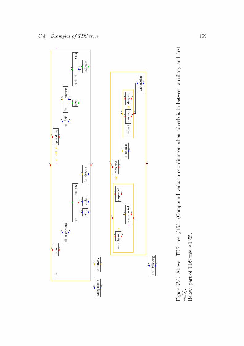
C.4. Examples of TDS trees 159
Der
egul
atio
n
has
effe
ctiv
ely
rem
oved
all
rest
rict
ions
on
wha
tba
nks
can
pay
for
depo
sits
,as
wel
las
open
edup
the
fiel
dfo
r
new
prod
ucts
such
as
high
-rat
e
CD
s
.
N N
V VA A
V VN N
J VN N
N N
A N
V VN N
A NJ J
J NJ J
The
follo
win
g
wer
eba
rred
or
,w
here
note
d,
susp
ende
dan
dco
nsen
ted
tofi
ndin
gsw
ithou
tad
mitt
ing
orde
nyin
g
wro
ngdo
ing
:
Edw
ard
L.
Col
e,
Jack
son
,
Mis
s.
,
$
10,0
00
fine
;R
itaR
aeC
ross
,
Den
ver
,
$
2,50
0
fine
and
30-d
ay
susp
ensi
on
;T
hom
asR
icha
rdM
eind
ers
,
Col
orad
oSp
ring
s,
Col
o.
,
$
2,00
0
fine
,
five
-day
susp
ensi
onan
d
eigh
t-m
onth
susp
ensi
on
asa
prin
cipa
l
;R
onal
dA
.C
utre
r,
Bat
onR
ouge
,
La.
,
$
15,0
00
fine
and
one-
mon
th
susp
ensi
on
;K
arl
Gra
ntH
ale
,
Mid
vale
,
Uta
h
,
$
15,0
00
fine
;C
linto
nP.
Hay
ne,
New
Orl
eans
,
$
7,50
0
fine
and
one-
wee
k
susp
ensi
on
;R
icha
rdM
.K
ane
,
Coc
onut
Cre
ek,
Fla.
,
$
250,
000
fine
;Jo
hnB
.M
erri
ck,
Aur
ora
,
Col
o.
,
$
1,00
0
fine
and
10-d
ay
susp
ensi
on
;Jo
hnP.
Mill
er,
Bat
onR
ouge
,
$
2,00
0
fine
and
two-
wee
k
susp
ensi
on
;R
ando
lph
K.
Pace
,
New
Yor
k
,
$
10,0
00
fine
and
90-d
ay
susp
ensi
on
;B
rian
D.
Pitc
her
,
New
Prov
iden
ce,
N.J
.
,
$
30,0
00
fine
;W
ayne
A.
Rus
so,
Bri
dgev
ille
,
Pa.
,
$
4,00
0
fine
and
15-d
ay
susp
ensi
on
;O
rvill
eL
eroy
Sand
berg
,
Aur
ora
,
Col
o.
,
$
3,50
0
fine
and
10-d
ay
susp
ensi
on
;R
icha
rdT
.M
arch
ese
,
Las
Veg
as,
Nev
.
,
$
5,00
0
and
one-
year
susp
ensi
on
;E
ric
G.
Mon
chec
ourt
,
Las
Veg
as
,
$
5,00
0
and
one-
year
susp
ensi
on
;an
dR
ober
tG
erha
rdSm
ith,
Car
son
City
,
Nev
.
,
two-
year
susp
ensi
on
.
N N
V V
V V
V VA V
V V
V VA N
A V
V V
V V
N N
N N
N N
J NJ N
J NJ J
J N
N NJ N
J NJ J
J N
J N
J J
J N
N NJ N
J N
J NJ J
J N
J N
J J
J NJ J
J NJ N
N NJ N
J N
J NJ J
J N
J N
J J
J N
N NJ N
J N
J NJ J
J N
N NJ N
J NJ J
J N
J N
J J
J N
N NJ N
J N
J NJ J
J N
N NJ N
J N
J NJ J
J N
J N
J J
J N
N NJ N
J NJ J
J N
J N
J J
J N
N NJ N
J NJ J
J N
J N
J J
J N
N NJ N
J N
J NJ J
J N
N NJ N
J N
J NJ J
J N
J N
J J
J N
N NJ N
J N
J NJ J
J N
J N
J J
J N
N NJ N
J N
J N
J N
J J
J J
J N
N NJ N
J N
J N
J J
J J
J N
N NJ N
J N
J J
J N
Figu
reC
.6:
Abo
ve:
TD
Str
ee#
1531
(Com
poun
dve
rbs
inco
ordi
natio
nw
hen
adve
rbis
inbe
twee
nau
xilia
ryan
dfir
stve
rb).
Belo
w:
part
ofT
DS
tree
#18
55.


Bibliography
Abeille, Anne. Treebanks: Building and Using Parsed Corpora, volume 20 of Text,Speech and Language Technology. Kluwer Academic Publishers, 2003.
Abeille, Anne, Lionel Clement, and Francois Toussenel. Building a Treebank forFrench, pages 165–188. Volume 20 of Text, Speech and Language TechnologyAbeille (2003), 2003.
Abend, Omri and Ari Rappoport. Fully unsupervised core-adjunct argumentclassification. In Proceedings of the 48th Annual Meeting of the Association forComputational Linguistics, ACL ’10, pages 226–236, Stroudsburg, PA, USA,2010. Association for Computational Linguistics.
Abney, Steven. Statistical Methods and Linguistics. In Klavans, Judith and PhilipResnik, editors, The Balancing Act: Combining Symbolic and Statistical Ap-proaches to Language, pages 1–26. The MIT Press, Cambridge, Massachusetts,1996.
Aho, A. V. and S. C. Johnson. LR Parsing. ACM Comput. Surv., 6(2):99–124,1974.
Ajdukiewicz, K. Die syntaktische Konnexitat. Studia Philosophica, 1:1–27, 1935.
Anderson, John. Dependency and Grammatical Functions. Foundations of Lan-guage, 7(1):pp. 30–37, 1971.
Arnon, Inbal. Starting big — The role of multi-word phrases in language learningand use. PhD thesis, Stanford University, 2009.
Arnon, Inbal and Neal Snider. More than words: Frequency effects for multi-wordphrases. Journal of Memory and Language, 62(1):67–82, 2010.
161

162 BIBLIOGRAPHY
Arun, Abhishek and Frank Keller. Lexicalization in crosslinguistic probabilisticparsing: the case of French. In Proceedings of the 43rd Annual Meeting on As-sociation for Computational Linguistics, ACL ’05, pages 306–313, Stroudsburg,PA, USA, 2005. Association for Computational Linguistics.
Bachrach, Asaf. Imaging neural correlates of syntactic complexity in a naturalisticcontext. PhD thesis, Massachusetts Institute of Technology, 2008.
Back, E., S. Abney, D. Flickenger, C. Gdaniec, R. Grishman, P. Harrison, D. Hin-dle, R. Ingria, F. Jelinek, J. Klavans, M. Liberman, M. Marcus, S. Roukos,B. Santorini, and T. Strzalkowski. A procedure for quantitatively compar-ing the syntactic coverage of English grammars. In Proceedings of the FourthDARPA Speech and Natural Language Workshop, pages 306–311, 1991.
Baldwin, Timothy and Valia Kordoni, editors. Proceedings of the EACL 2009Workshop on the Interaction between Linguistics and Computational Linguis-tics: Virtuous, Vicious or Vacuous? Association for Computational Linguis-tics, Athens, Greece, March 2009.
Bangalore, Srinivas, Pierre Boullier, Alexis Nasr, Owen Rambow, and BenoıtSagot. MICA: A Probabilistic Dependency Parser Based on Tree InsertionGrammars (Application Note). In Proceedings of Human Language Technolo-gies: The 2009 Annual Conference of the North American Chapter of the As-sociation for Computational Linguistics, Companion Volume: Short Papers,pages 185–188, Boulder, Colorado, June 2009. Association for ComputationalLinguistics.
Bansal, Mohit and Dan Klein. Simple, Accurate Parsing with an All-FragmentsGrammar. In Proceedings of the 48th Annual Meeting of the Association forComputational Linguistics, pages 1098–1107, Uppsala, Sweden, July 2010. As-sociation for Computational Linguistics.
Bansal, Mohit and Dan Klein. Web-scale features for full-scale parsing. In Pro-ceedings of the 49th Annual Meeting of the Association for Computational Lin-guistics: Human Language Technologies - Volume 1, HLT ’11, pages 693–702,Stroudsburg, PA, USA, 2011. Association for Computational Linguistics.
Bar-Hillel, Yehoshua. A quasi-arithmetical notation for syntactic description.Language, 29(1):47–58, 1953.
Bauer, Laurie. Some thoughts on dependency grammar. Linguistics, 17:301–316,1979.
Berger, Adam L., Vincent J. Della Pietra, and Stephen A. Della Pietra. A maxi-mum entropy approach to natural language processing. Comput. Linguist., 22(1):39–71, 1996.

BIBLIOGRAPHY 163
Bikel, Daniel M. Intricacies of Collins’ Parsing Model. Comput. Linguist., 30(4):479–511, 2004a.
Bikel, Daniel M. On the parameter space of generative lexicalized statistical pars-ing models. PhD thesis, University of Pennsylvania, Philadelphia, PA, USA,2004b. Supervisor-Marcus, Mitchell P.
Bloomfield, Leonard. Language. New York: Holt, 1933.
Blunsom, Phil and Trevor Cohn. Unsupervised induction of tree substitutiongrammars for dependency parsing. In Proceedings of the 2010 Conference onEmpirical Methods in Natural Language Processing, EMNLP ’10, pages 1204–1213, Stroudsburg, PA, USA, 2010. Association for Computational Linguistics.
Bod, Rens. A Computational Model of Language Performance: Data OrientedParsing. In Proceedings COLING’92 (Nantes, France), pages 855–859. Associ-ation for Computational Linguistics, Morristown, NJ, 1992.
Bod, Rens. Using an Annotated Language Corpus as a Virtual Stochastic Gram-mar. In AAAI, pages 778–783, 1993.
Bod, Rens. Combining semantic and syntactic structure for language modeling.CoRR, cs.CL/0110051, 2001a.
Bod, Rens. What is the Minimal Set of Fragments that Achieves Maximal ParseAccuracy? In Proceedings ACL-2001. Morgan Kaufmann, San Francisco, CA,2001b.
Bod, Rens. An efficient implementation of a new DOP model. In Proceedings ofthe tenth conference on European chapter of the Association for ComputationalLinguistics - Volume 1, EACL ’03, pages 19–26, Morristown, NJ, USA, 2003.Association for Computational Linguistics.
Bod, Rens. Unsupervised parsing with U-DOP. In CoNLL-X ’06: Proceedingsof the Tenth Conference on Computational Natural Language Learning, pages85–92, Morristown, NJ, USA, 2006. Association for Computational Linguistics.
Bod, Rens and Ronald Kaplan. Data-Oriented Parsing, chapter A Data-OrientedParsing Model for Lexical-Functional Grammar. In Bod et al. (2003), 2003.
Bod, Rens, Khalil Sima’an, and Remko Scha. Data-Oriented Parsing. Universityof Chicago Press, Chicago, IL, USA, 2003.
Boersma, P. and B. Hayes. Empirical tests of the gradual learning algorithm.Linguistic Inquiry, 32(1):45–86, 2001.

164 BIBLIOGRAPHY
Bonnema, Remko, Rens Bod, and Remko Scha. A DOP model for semanticinterpretation. In Proceedings of the 35th Annual Meeting of the Associationfor Computational Linguistics and Eighth Conference of the European Chap-ter of the Association for Computational Linguistics, ACL ’98, pages 159–167,Stroudsburg, PA, USA, 1997. Association for Computational Linguistics.
Bonnema, Remko, Paul Buying, and Remko Scha. A New Probability Modelfor Data Oriented Parsing, volume Proceedings of the Twelfth AmsterdamColloquium, pages 85–90. 1999.
Borensztajn, Gideon and Willem Zuidema. Episodic grammar: a computationalmodel of the interaction between episodic and semantic memory in languageprocessing. In Proceedings of the 33rd Cognitive Science Conference, 2011.
Borensztajn, Gideon, Willem Zuidema, and Rens Bod. Children’s GrammarsGrow More Abstract with Age—Evidence from an Automatic Procedure forIdentifying the Productive Units of Language. Topics in Cognitive Science, 1(1):175–188, January 2009.
Bosco, Cristina, Vincenzo Lombardo, Daniela Vassallo, and Leonardo Lesmo.Building a Treebank for Italian: a Data-driven Annotation Schema. In Pro-ceedings of the Second International Conference on Language Resources andEvaluation LREC-2000, pages 99–105, 2000.
Boser, Bernhard E., Isabelle M. Guyon, and Vladimir N. Vapnik. A trainingalgorithm for optimal margin classifiers. In COLT ’92: Proceedings of the fifthannual workshop on Computational learning theory, pages 144–152, New York,NY, USA, 1992. ACM.
Brants, Sabine, Stefanie Dipper, Silvia Hansen, Wolfgang Lezius, and GeorgeSmith. The TIGER Treebank. In Proceedings of the Workshop on Treebanksand Linguistic Theories, pages 24–41, 2002.
Bresnan, Joan. Lexical-Functional Syntax. Blackwell Textbooks in Linguistics.Blackwell Publishers, September 2000.
Buchanan, Bruce G. Mechanizing the Search for Explanatory Hypotheses. PSA:Proceedings of the Biennial Meeting of the Philosophy of Science Association,1982:pp. 129–146, 1982.
Buchholz, Sabine and Erwin Marsi. CoNLL-X shared task on multilingual de-pendency parsing. In In Proc. of CoNLL, pages 149–164, 2006.
Buchholz, Sabine, Jorn Veenstra, and Walter Daelemans. Cascaded GrammaticalRelation Assignment. In EMNLP/VLC-99, pages 239–246. ACL, 1999.
BIBLIOGRAPHY 165
Charniak, Eugene. Tree-bank Grammars. In In Proceedings of the ThirteenthNational Conference on Artificial Intelligence, pages 1031–1036, 1996.
Charniak, Eugene. Statistical Parsing with a Context-free Grammar and WordStatistics. In Proceedings of the Fourteenth National Conference on ArtificialIntelligence, pages 598–603. AAAI Press/MIT Press, 1997.
Charniak, Eugene. A Maximum-Entropy-Inspired Parser. Technical report,Brown University, Providence, RI, USA, 1999.
Charniak, Eugene and Mark Johnson. Coarse-to-Fine n-Best Parsing and MaxEntDiscriminative Reranking. In Proc. 43nd Meeting of Association for Computa-tional Linguistics (ACL 2005), 2005.
Chiang, David and Daniel M. Bikel. Recovering latent information in treebanks.In Proceedings of the 19th international conference on Computational linguis-tics, pages 1–7, Morristown, NJ, USA, 2002. Association for ComputationalLinguistics.
Chomsky, N. Three models for the description of language. Information Theory,IRE Transactions on, 2(3):113–124, January 1956.
Chomsky, N. Aspects of the theory of syntax. The MIT Press Paperback Series.M.I.T. Press, 1965.
Chomsky, N. Modular approaches to the study of the mind. Distinguished graduateresearch lecture. San Diego State University Press, 1984.
Chomsky, Noam. Syntactic structures. Mouton, Den Haag, 1957.
Chomsky, Noam. Remarks on nominalization. In Jacobs, R. and P. Rosenbaum,editors, Reading in English Transformational Grammar, pages 184–221. Ginnand Co., Waltham, 1970.
Cinkova, Silvie, Eva Hajicova, Jarmila Panevova, and Petr Sgall. Two Languages– One Annotation Scenario? Experience from the Prague Dependency Tree-bank. The Prague Bulletin of Mathematical Linguistics, (89):5—22, June 2008.
Cinkova, Silvie, Josef Toman, Jan Hajic, Kristyna Cermakova, Vaclav Klimes,Lucie Mladova, Jana Sindlerova, Kristyna Tomsu, and Zdenek Zabokrtsky.Tectogrammatical Annotation of the Wall Street Journal. The Prague Bulletinof Mathematical Linguistics, (92):85—104, December 2009.
Clark, Stephen and James Curran. Formalism-Independent Parser Evaluationwith CCG and DepBank. In Proceedings of the 45th Annual Meeting of theAssociation of Computational Linguistics, pages 248–255, Prague, Czech Re-public, June 2007a. Association for Computational Linguistics.

166 BIBLIOGRAPHY
Clark, Stephen and James R. Curran. Wide-coverage efficient statistical parsingwith ccg and log-linear models. Comput. Linguist., 33(4):493–552, 2007b.
Cohn, Trevor, Sharon Goldwater, and Phil Blunsom. Inducing Compact but Ac-curate Tree-Substitution Grammars. In Proceedings of Human Language Tech-nologies: The 2009 Annual Conference of the North American Chapter of theAssociation for Computational Linguistics, pages 548–556, Boulder, Colorado,June 2009. Association for Computational Linguistics.
Cohn, Trevor, Phil Blunsom, and Sharon Goldwater. Inducing Tree-SubstitutionGrammars. Journal of Machine Learning Research, 11:3053–3096, 2010.
Collins, Michael. Three generative, lexicalised models for statistical parsing. InACL-35: Proceedings of the 35th Annual Meeting of the Association for Com-putational Linguistics and Eighth Conference of the European Chapter of theAssociation for Computational Linguistics, pages 16–23, Morristown, NJ, USA,1997. Association for Computational Linguistics.
Collins, Michael. Discriminative Reranking for Natural Language Parsing. InICML ’00: Proceedings of the Seventeenth International Conference on Ma-chine Learning, pages 175–182, San Francisco, CA, USA, 2000. Morgan Kauf-mann Publishers Inc.
Collins, Michael and Nigel Duffy. Convolution Kernels for Natural Language.In Dietterich, Thomas G., Suzanna Becker, and Zoubin Ghahramani, editors,NIPS, pages 625–632. MIT Press, 2001.
Collins, Michael and Nigel Duffy. New Ranking Algorithms for Parsing and Tag-ging: Kernels over Discrete Structures, and the Voted Perceptron. In Proceed-ings of 40th Annual Meeting of the Association for Computational Linguistics,pages 263–270, Philadelphia, Pennsylvania, USA, July 2002. Association forComputational Linguistics.
Collins, Michael and Terry Koo. Discriminative Reranking for Natural LanguageParsing. Comput. Linguist., 31(1):25–70, 2005.
Collins, Michael and Brian Roark. Incremental parsing with the perceptron algo-rithm. In ACL ’04: Proceedings of the 42nd Annual Meeting on Association forComputational Linguistics, page 111, Morristown, NJ, USA, 2004. Associationfor Computational Linguistics.
Collins, Michael J. Head-Driven Statistical Models for Natural Language Parsing.PhD thesis, University of Pennsylvania, 1999.
BIBLIOGRAPHY 167
Collins, Michael John. A new statistical parser based on bigram lexical depen-dencies. In Proceedings of the 34th annual meeting on Association for Compu-tational Linguistics, pages 184–191, Morristown, NJ, USA, 1996. Associationfor Computational Linguistics.
Corbett, Greville G., Norman M. Fraser, and Scott McGlashan. Heads in Gram-matical Theory. Cambridge University Press, New York, 2006.
Covington, Michael A. GB Theory as Dependency Grammar. Technical ReportAI-1992-03, University of Georgia, Athens, Georgia, 1992.
Daelemans, Walter, Sabine Buchholz, and Jorn Veenstra. Memory-based ShallowParsing. In Proceedings of CoNLL-1999, Bergen, Norway, 1999.
Dalrymple, Mary. Lexical-Functional Grammar (Syntax and Semantics). Aca-demic Press, 2001.
Daume III, Hal and Daniel Marcu. NP Bracketing by Maximum Entropy Taggingand SVM Reranking. In The 2004 Conference on Empirical Methods in NaturalLanguage Processing, pages 254–261, 2004.
De Marneffe, Marie-Catherin, Bill Maccartney, and Christopher D. Manning.Generating typed dependency parses from phrase structure parses. In In LREC2006, 2006.
De Marneffe, Marie-Catherine and Christopher D. Manning. The Stanford TypedDependencies Representation. In Coling 2008: Proceedings of the workshop onCross-Framework and Cross-Domain Parser Evaluation, pages 1–8, Manch-ester, UK, August 2008. Coling 2008 Organizing Committee.
de Saussure, Ferdenand. Course in General Linguistics. McGraw Hill, New York,1915.
Dinarelli, Marco, Alessandro Moschitti, and Giuseppe Riccardi. Re-ranking mod-els for spoken language understanding. In EACL ’09: Proceedings of the 12thConference of the European Chapter of the Association for Computational Lin-guistics, pages 202–210, Morristown, NJ, USA, 2009. Association for Compu-tational Linguistics.
Dubey, Amit. What to do when lexicalization fails: parsing German with suffixanalysis and smoothing. In Proceedings of the 43rd Annual Meeting on Asso-ciation for Computational Linguistics, ACL ’05, pages 314–321, Stroudsburg,PA, USA, 2005. Association for Computational Linguistics.
Eisner, Jason. Bilexical Grammars And A Cubic-Time Probabilistic Parser. InIn Proceedings of the International Workshop on Parsing Technologies, pages54–65, 1997.

168 BIBLIOGRAPHY
Eisner, Jason. Bilexical Grammars and Their Cubic-Time Parsing Algorithms. InBunt, Harry and Anton Nijholt, editors, Advances in Probabilistic and OtherParsing Technologies, pages 29–62. Kluwer Academic Publishers, October 2000.
Eisner, Jason and Giorgio Satta. Efficient parsing for bilexical context-free gram-mars and head automaton grammars. In Proceedings of the 37th annual meetingof the Association for Computational Linguistics on Computational Linguistics,ACL ’99, pages 457–464, Stroudsburg, PA, USA, 1999. Association for Com-putational Linguistics.
Eisner, Jason M. An Empirical Comparison of Probability Models for DependencyGrammar. Technical Report IRCS-96-11, University of Pennsylvania, 1996a.
Eisner, Jason M. Three new probabilistic models for dependency parsing: anexploration. In Proceedings of the 16th conference on Computational linguistics,pages 340–345, Morristown, NJ, USA, 1996b. Association for ComputationalLinguistics.
Fillmore, Charles J., Paul Kay, and Mary C. O’Connor. Regularity and Idiomatic-ity in Grammatical Constructions: The Case of Let Alone. Language, 64(3):501–538, 1988.
Forst, Martin, Nuria Bertomeu, Berthold Crysmann, Frederik Fouvry, SilviaHansen-Schirra, and Valia Kordoni. Towards a dependency-based gold stan-dard for German parsers - The TiGer Dependency Bank, 2004.
Frank, Stefan L and Rens Bod. Insensitivity of the human sentence-processingsystem to hierarchical structure. Psychological Science, (May), 2011.
Fraser, Alexander, Renjing Wang, and Hinrich Schutze. Rich bitext projectionfeatures for parse reranking. In EACL ’09: Proceedings of the 12th Confer-ence of the European Chapter of the Association for Computational Linguistics,pages 282–290, Morristown, NJ, USA, 2009. Association for ComputationalLinguistics.
Frazier, Lyn. On Comprehending Sentences: Syntactic Parsing Strategies. PhDthesis, University of Massachusetts, Indiana University Linguistics Club, 1979.
Gaifman, Haim. Dependency systems and phrase-structure systems. Informationand Control, 8(3):304 – 337, 1965.
Goldberg, A.E. Constructions: A Construction Grammar Approach to ArgumentStructure. University Of Chicago Press, 1995.

BIBLIOGRAPHY 169
Goldwater, Sharon, Thomas L. Griffiths, and Mark Johnson. Distributional Cuesto Word Boundaries: Context is Important. In Bamman, David, Tatiana Mag-nitskaia, and Colleen Zaller, editors, Proceedings of the 31st Annual BostonUniversity Conference on Language Development, pages 239—250, 2007.
Goldwater, Sharon, Thomas L. Griffiths, and Mark Johnson. A Bayesian frame-work for word segmentation: Exploring the effects of context. Cognition, 112(1):21–54, 2009.
Goodman, Joshua. Efficient algorithms for parsing the DOP model. In Proceed-ings of the Conference on Empirical Methods in Natural Language Processing,pages 143–152, 1996.
Goodman, Joshua. Probabilistic Feature Grammars. In In Proceedings of theInternational Workshop on Parsing Technologies, pages 89–100, 1997.
Goodman, Joshua. Data-Oriented Parsing, chapter Efficient Parsing of DOP withPCFG-Reductions. In Bod et al. (2003), 2003.
Goodman, Joshua T. Parsing inside-out. PhD thesis, Harvard University, Cam-bridge, MA, USA, 1998. Adviser-Shieber, Stuart.
Hajic, Jan, Alena Bohmova, Eva Hajicova, and Barbora Vidova-Hladka. ThePrague Dependency Treebank: A Three-Level Annotation Scenario. In Abeille,A., editor, Treebanks: Building and Using Parsed Corpora, pages 103–127. Am-sterdam:Kluwer, 2000.
Hale, John. Uncertainty About the Rest of the Sentence. Cognitive Science, 30:643–672, 2006.
Hall, Johan, Joakim Nivre, and Jens Nilsson. Discriminative Classifiers for De-terministic Dependency Parsing. In ACL. The Association for Computer Lin-guistics, 2006.
Hall, Keith, Jiri Havelka, and David A. Smith. Log-Linear Models of Non-Projective Trees, k-best MST Parsing and Tree-Ranking. In Proceedings of theCoNLL Shared Task Session of EMNLP-CoNLL 2007, pages 962–966, Prague,Czech Republic, June 2007. Association for Computational Linguistics.
Harris, Zelig S. Structural Linguistics. University of Chicago Press, 1951.
Hays, David G. Grouping and dependency theories. In National Symposium onMachine Translation, pages 258–266, Englewood Cliffs, NY, USA, 1960.
Hays, David G. Dependency Theory: A Formalism and Some Observations.Language, 40(4):pp. 511–525, 1964.
170 BIBLIOGRAPHY
Hearne, Mary and Andy Way. Disambiguation Strategies for Data-OrientedTranslation. In Proceedings of the 11th Conference of the European Associ-ation for Machine Translation, pages 59–68, 2006.
Heringer, James T. Review of Gaifman (1965). Ohio State University WorkingPapers in Linguistics, 1967.
Hockenmaier, Julia. Data and models for statistical parsing Data and models forstatistical parsing with Combinatory Categorial Grammar. PhD thesis, Univer-sity of Edinburgh, 2003.
Hockenmaier, Julia and Mark Steedman. CCGbank: A Corpus of CCG Deriva-tions and Dependency Structures Extracted from the Penn Treebank. Compu-tational Linguistics, 33(3):355–396, 2007.
Huang, Liang. Forest Reranking: Discriminative Parsing with Non-Local Fea-tures. In Proceedings of ACL-08: HLT, pages 586–594, Columbus, Ohio, June2008. Association for Computational Linguistics.
Hudson, R.A. English word grammar. B. Blackwell, 1991.
Hudson, Richard. An Introduction to Word Grammar. Cambridge UniversityPress, 2010.
Hudson, Rodney. Zwicky on heads. Journal of Linguistics, 23:109–132, 1987.
Hurford, James R. Human uniqueness, learned symbols and recursive thought.European Review, 12(04):551–565, October 2004.
Hwa, Rebecca. An empirical evaluation of Probabilistic Lexicalized Tree InsertionGrammars. In Proceedings of the 17th international conference on Computa-tional linguistics, pages 557–563, Morristown, NJ, USA, 1998. Association forComputational Linguistics.
Jackendoff, Ray. Foundations of Language. Oxford University Press, Oxford, UK,2002.
Jackendoff, Ray S. X Syntax: A Study of Phrase Structure. The MIT Press,Cambridge, MA, 1977.
Jespersen, Otto. Analytic syntax. London, 1937.
Johansson, Richard and Pierre Nugues. Extended Constituent-to-DependencyConversion for English. In Proceedings of NODALIDA 2007, Tartu, Estonia,May 2007.
Johnson, Mark. PCFG models of linguistic tree representations. Comput. Lin-guist., 24(4):613–632, 1998.

BIBLIOGRAPHY 171
Johnson, Mark. Transforming Projective Bilexical Dependency Grammars intoefficiently-parsable CFGs with Unfold-Fold. In Proceedings of the 45th An-nual Meeting of the Association of Computational Linguistics, pages 168–175,Prague, Czech Republic, June 2007. Association for Computational Linguistics.
Johnson, Mark. How the Statistical Revolution Changes (Computational) Lin-guistics. In Proceedings of the EACL 2009 Workshop on the Interaction be-tween Linguistics and Computational Linguistics: Virtuous, Vicious or Vacu-ous?, pages 3–11, Athens, Greece, March 2009. Association for ComputationalLinguistics.
Johnson, Mark and Ahmet Engin Ural. Reranking the Berkeley and BrownParsers. In Human Language Technologies: The 2010 Annual Conference ofthe North American Chapter of the Association for Computational Linguistics,pages 665–668, Los Angeles, California, June 2010. Association for Computa-tional Linguistics.
Johnson, Mark, Thomas Griffiths, and Sharon Goldwater. Bayesian Inferencefor PCFGs via Markov Chain Monte Carlo. In Human Language Technologies2007: The Conference of the North American Chapter of the Association forComputational Linguistics; Proceedings of the Main Conference, pages 139–146,Rochester, New York, April 2007a. Association for Computational Linguistics.
Johnson, Mark, Thomas L. Griffiths, and Sharon Goldwater. Adaptor Grammars:A Framework for Specifying Compositional Nonparametric Bayesian Models.In Advances in Neural Information Processing Systems, volume 16, pages 641–648, 2007b.
Joshi, Aravind K. Tree-adjoining grammars: How much context sensitivity is re-quired to provide reasonable structural descriptions. In Dowty, D. R., L. Kart-tunen, and A. Zwicky, editors, Natural Language Parsing, chapter 6, pages206–250. Cambridge University Press, New York, 1985.
Joshi, Aravind K. and Yves Schabes. Tree-adjoining grammars and lexicalizedgrammars. In Nivat, Maurice and Andreas Podelski, editors, Definability andRecognizability of Sets of Trees. Elsevier, 1991.
Kahane, Sylvain. Bubble trees and syntactic representations. In Krieger,Becker &, editor, Proceedings 5th Meeting of the Mathematics of Language(MOL5). Saarbrucken: DFKI, 1997.
Kahane, Sylvain. Polarized Unification Grammars. In Proceedings of the 21st In-ternational Conference on Computational Linguistics and 44th Annual Meetingof the Association for Computational Linguistics, pages 137–144, Sydney, Aus-tralia, July 2006. Association for Computational Linguistics.

172 BIBLIOGRAPHY
Kaplan, R. M. and J. Bresnan. Lexical-Functional Grammar: A Formal Systemfor Grammatical Representation. In Bresnan, J., editor, The Mental Represen-tation of Grammatical Relations, pages 173–281. MIT Press, Cambridge, MA,1982.
Kay, Paul and Charles J. Fillmore. Grammatical Constructions and LinguisticGeneralizations: the What’s X Doing Y? Construction. Language, 75:1–33,1997.
Klavans, Judith L. and Philip Resnik, editors. The Balancing Act: combiningsymbolic and statistical approaches to language. MIT Press, Cambridge, MA,1996.
Klein, Dan. The unsupervised learning of natural language structure. PhD thesis,Stanford University, Stanford, CA, USA, 2005. Adviser-Manning, ChristopherD.
Klein, Dan and Christopher D. Manning. Accurate unlexicalized parsing. InACL ’03: Proceedings of the 41st Annual Meeting on Association for Compu-tational Linguistics, pages 423–430, Morristown, NJ, USA, 2003. Associationfor Computational Linguistics.
Kuhlmann, Marco. Dependency Structures and Lexicalized Grammars. PhD the-sis, Saarland University, Saarbrucken, Germany, 2007.
Labov, William, editor. Sociolinguistic Patterns. University of Philadelphia Press,Philadelphia, 1972.
Lapata, Mirella and Frank Keller. The Web as a Baseline: Evaluating the Per-formance of Unsupervised Web-based Models for a Range of NLP Tasks. InSusan Dumais, Daniel Marcu and Salim Roukos, editors, HLT-NAACL 2004:Main Proceedings, pages 121–128, Boston, Massachusetts, USA, May 2 - May7 2004. Association for Computational Linguistics.
Lari, K. and S. J. Young. The estimation of stochastic context-free grammarsusing the Inside-Outside algorithm. Computer Speech and Language, 4:35–56,1990.
Lass, Roger. Historical Linguistics and Language Change. Cambridge UniversityPress, New York, 1997.
Levelt, W.J.M. Formal grammars in linguistics and psycholinguistics: Appli-cations in Linguistic Theory, volume 2 of Janua linguarum: Series minor.Mouton, 1974.
Levy, Roger. Expectation-based syntactic comprehension. Cognition, July 2007.

BIBLIOGRAPHY 173
Lieberman, P. On the origins of language: an introduction to the evolution ofhuman speech. Macmillan series in physical anthropology. Macmillan, 1975.
Lieven, Elena, Heike Behrens, Jennifer Speares, and Michael Tomasello. Earlysyntactic creativity: a usage-based approach. Journal of Child Language, 30(2):333–370, 2003.
Lin, Dekang. A Dependency-based Method for Evaluating Broad-CoverageParsers. In In Proceedings of IJCAI-95, pages 1420–1425, 1995.
Lindsay, Robert K., Bruce G. Buchanan, E. A. Feigenbaum, and Joshua Leder-berg. Applications of Artificial Intelligence for Organic Chemistry: The DEN-DRAL Project. McGraw-Hill Companies, Inc, 1980.
Magerman, David M. Natural Language Parsing as Statistical Pattern Recogni-tion. PhD thesis, Stanford University, 1994.
Magerman, David M. Statistical Decision-Tree Models for Parsing. In Proceedingsof the 33rd Annual Meeting of the Association for Computational Linguistics,pages 276–283, Cambridge, Massachusetts, USA, June 1995. Association forComputational Linguistics.
Marcus, Mitchell, Grace Kim, Mary Ann Marcinkiewicz, Robert MacIntyre, AnnBies, Mark Ferguson, Karen Katz, and Britta Schasberger. The Penn Tree-bank: annotating predicate argument structure. In HLT ’94: Proceedings ofthe workshop on Human Language Technology, pages 114–119, Morristown, NJ,USA, 1994. Association for Computational Linguistics.
Marcus, Mitchell P., Mary Ann Marcinkiewicz, and Beatrice Santorini. Buildinga Large Annotated Corpus of English: The Penn Treebank. ComputationalLinguistics, 19(2):313–330, 1993.
Marcus, Mitchell P., Beatrice Santorini, Mary Ann Marcinkiewicz, and AnnsTaylor. Treebank-3. Linguistic Data Consortium, Philadelphia, 1999.
Martin, William A., Kenneth W. Church, and Ramesh S. Patil. Preliminary anal-ysis of a breadth-first parsing algorithm: theoretical and experimental results.Natural language parsing systems, pages 267–328, 1987.
Matsuzaki, Takuya, Yusuke Miyao, and Jun’ichi Tsujii. Probabilistic CFG withlatent annotations. In ACL ’05: Proceedings of the 43rd Annual Meeting onAssociation for Computational Linguistics, pages 75–82, Morristown, NJ, USA,2005. Association for Computational Linguistics.
McClosky, David, Eugene Charniak, and Mark Johnson. Reranking and self-training for parser adaptation. In ACL-44: Proceedings of the 21st International
174 BIBLIOGRAPHY
Conference on Computational Linguistics and the 44th annual meeting of theAssociation for Computational Linguistics, pages 337–344, Morristown, NJ,USA, 2006. Association for Computational Linguistics.
McDonald, Ryan. Discriminative learning and spanning tree algorithms for de-pendency parsing. PhD thesis, University of Pennsylvania, Philadelphia, PA,USA, 2006.
McDonald, Ryan, Fernando Pereira, Kiril Ribarov, and Jan Hajic. Non-projectivedependency parsing using spanning tree algorithms. In HLT ’05: Proceedingsof the conference on Human Language Technology and Empirical Methods inNatural Language Processing, pages 523–530, Morristown, NJ, USA, 2005. As-sociation for Computational Linguistics.
Mel’cuk, Igor. Dependency Syntax: Theory and Practice. State University of NewYork Press, 1988.
Mel’cuk, Igor. Levels of Dependency in Linguistic Description: Concepts andProblems. Unpublished manuscript, 2003.
Mel’cuk, Igor A. Studies in dependency syntax. Karoma Publishers, Ann Arbor,1979.
Mitchell, Jeff and Mirella Lapata. Language Models Based on Semantic Compo-sition. In Proceedings of the 2009 Conference on Empirical Methods in NaturalLanguage Processing, pages 430–439, Singapore, 2009.
Moschitti, Alessandro. Efficient Convolution Kernels for Dependency and Con-stituent Syntactic Trees. In ECML, pages 318–329, Berlin, Germany, Septem-ber 2006. Machine Learning: ECML 2006, 17th European Conference on Ma-chine Learning, Proceedings.
Mylonakis, Markos and Khalil Sima’an. Phrase translation probabilities with ITGpriors and smoothing as learning objective. In Proceedings of the Conference onEmpirical Methods in Natural Language Processing, EMNLP ’08, pages 630–639, Stroudsburg, PA, USA, 2008. Association for Computational Linguistics.
Ng, Andrew Y. and Michael I. Jordan. On Discriminative vs. Generative Clas-sifiers: A comparison of logistic regression and naive Bayes. In NIPS, pages841–848, 2001.
Nivre, Joakim. An Efficient Algorithm for Projective Dependency Parsing. InEighth International Workshop on Parsing Technologies, Nancy, France, 2003.
Nivre, Joakim. Inductive Dependency Parsing (Text, Speech and Language Tech-nology). Springer-Verlag New York, Inc., Secaucus, NJ, USA, 2006.

BIBLIOGRAPHY 175
Nivre, Joakim. Non-Projective Dependency Parsing in Expected Linear Time.In Proceedings of the Joint Conference of the 47th Annual Meeting of the ACLand the 4th International Joint Conference on Natural Language Processing ofthe AFNLP, pages 351–359, Suntec, Singapore, August 2009. Association forComputational Linguistics.
Nivre, Joakim and Jens Nilsson. Pseudo-Projective Dependency Parsing. In ACL.The Association for Computer Linguistics, 2005.
Nivre, Joakim, Johan Hall, Sandra Kubler, Ryan Mcdonald, Jens Nilsson, Sebas-tian Riedel, and Deniz Yuret. The CoNLL 2007 Shared Task on DependencyParsing. In Proceedings of the CoNLL Shared Task Session of EMNLP-CoNLL2007, pages 915–932, Prague, Czech Republic, June 2007. Association for Com-putational Linguistics.
O’Donnell, Timothy J., Noah D. Goodman, and Joshua B. Tenenbaum. FragmentGrammars: Exploring Computation and Reuse in Language. Technical ReportMIT-CSAIL-TR-2009-013, MIT, 2009.
Oflazer, Kemal, Bilge Say, Dilek Zeynep Hakkani-tur, and Gokhan Tur. BuildingA Turkish Treebank. In Abeille, A., editor, Treebanks: Building and UsingParsed Corpora, pages 261–277. Kluwer Academic Publishers, 2003.
Pereira, Fernando and Yves Schabes. Inside-outside reestimation from partiallybracketed corpora. In Proceedings of the 30th annual meeting on Associationfor Computational Linguistics, pages 128–135, Morristown, NJ, USA, 1992.Association for Computational Linguistics.
Petrov, Slav. Coarse-to-Fine Natural Language Processing. PhD thesis, Universityof California at Bekeley, Berkeley, CA, USA, 2009.
Petrov, Slav and Dan Klein. Improved Inference for Unlexicalized Parsing. InHuman Language Technologies 2007: The Conference of the North AmericanChapter of the Association for Computational Linguistics; Proceedings of theMain Conference, pages 404–411, Rochester, New York, April 2007. Associationfor Computational Linguistics.
Petrov, Slav, Leon Barrett, Romain Thibaux, and Dan Klein. Learning accurate,compact, and interpretable tree annotation. In ACL-44: Proceedings of the21st International Conference on Computational Linguistics and the 44th an-nual meeting of the Association for Computational Linguistics, pages 433–440,Morristown, NJ, USA, 2006. Association for Computational Linguistics.
Pinker, Stephen and Ray Jackendoff. The faculty of language: what’s specialabout it? Cognition, 95:201–236, 2005.
176 BIBLIOGRAPHY
Polguere, Alain and Igor A. Mel’cuk, editors. Dependency in Linguistic Descrip-tion. Studies in Language Companion Series 111. John Benjamins, Philadel-phia, 2009.
Pollard, Carl, , Carl Pollard, and Ivan A. Sag. Head-driven Phrase StructureGrammar. University of Chicago Press, 1994.
Post, Matt and Daniel Gildea. Bayesian Learning of a Tree Substitution Gram-mar. In Proceedings of the ACL-IJCNLP 2009 Conference Short Papers, pages45–48, Suntec, Singapore, August 2009. Association for Computational Lin-guistics.
Prescher, Detlef. A Tutorial on the Expectation-Maximization Algorithm In-cluding Maximum-Likelihood Estimation and EM Training of ProbabilisticContext-Free Grammars. In ESSLLI, 2003.
Prescher, Detlef. Inside-Outside Estimation Meets Dynamic EM. CoRR,abs/cs/0412016, 2004.
Prescher, Detlef. Head-driven PCFGs with latent-head statistics. In Parsing’05: Proceedings of the Ninth International Workshop on Parsing Technology,pages 115–124, Morristown, NJ, USA, 2005a. Association for ComputationalLinguistics.
Prescher, Detlef. Inducing head-driven PCFGs with latent heads: Refining atree-bank grammar for parsing. In In ECML’05, 2005b.
Ratnaparkhi, Adwait. A Linear Observed Time Statistical Parser Based on Max-imum Entropy Models. CoRR, cmp-lg/9706014, 1997.
Ratnaparkhi, Adwait. Learning to Parse Natural Language with Maximum En-tropy Models. Mach. Learn., 34(1-3):151–175, 1999.
Riezler, Stefan, Tracy H. King, Ronald M. Kaplan, Richard Crouch, John T.Maxwell, and Mark Johnson. Parsing the Wall Street Journal using a Lexical-Functional Grammar and Discriminative Estimation Techniques. In Proceed-ings of the 40th Annual Meeting of the Association for Computational Linguis-tics (ACL’02), Philadelphia, PA, USA, 2002.
Rimell, Laura, Stephen Clark, and Mark Steedman. Unbounded dependencyrecovery for parser evaluation. In EMNLP ’09: Proceedings of the 2009 Con-ference on Empirical Methods in Natural Language Processing, pages 813–821,Morristown, NJ, USA, 2009. Association for Computational Linguistics.
Robinson, Jane J. Methods for obtaining corresponding phrase structure anddependency grammars. In Proceedings of the 1967 conference on Computational
BIBLIOGRAPHY 177
linguistics, COLING ’67, pages 1–25, Stroudsburg, PA, USA, 1967. Associationfor Computational Linguistics.
Rosenblatt, F. The perceptron: a probabilistic model for information storage andorganization in the brain. Psychological Reviews, pages 386–408, 1958.
Sampson, Geoffrey, Robin Haigh, and Eric Atwell. Natural language analysis bystochastic optimization: a progress report on project APRIL. J. Exp. Theor.Artif. Intell., 1:271–287, October 1989.
Sangati, Federico. A Probabilistic Generative Model for an IntermediateConstituency-Dependency Representation. In Proceedings of the ACL 2010Student Research Workshop, pages 19–24, Uppsala, Sweden, July 2010. Asso-ciation for Computational Linguistics.
Sangati, Federico and Chiara Mazza. An English Dependency Treebank a laTesniere. In The 8th International Workshop on Treebanks and Linguistic The-ories, pages 173–184, Milan, Italy, 2009.
Sangati, Federico and Willem Zuidema. Unsupervised Methods for Head Assign-ments. In Proceedings of the 12th Conference of the European Chapter of theACL (EACL 2009), pages 701–709, Athens, Greece, March 2009. Associationfor Computational Linguistics.
Sangati, Federico and Willem Zuidema. A Recurring Fragment Model for Accu-rate Parsing: Double-DOP . In Proceedings of the 2011 Conference on Empiri-cal Methods in Natural Language Processing, pages 84–95, Edinburgh, Scotland,UK., July 2011. Association for Computational Linguistics.
Sangati, Federico, Willem Zuidema, and Rens Bod. A generative re-ranking modelfor dependency parsing. In Proceedings of the 11th International Conference onParsing Technologies (IWPT’09), pages 238–241, Paris, France, October 2009.Association for Computational Linguistics.
Sangati, Federico, Willem Zuidema, and Rens Bod. Efficiently Extract RecurringTree Fragments from Large Treebanks. In Chair), Nicoletta Calzolari (Con-ference, Khalid Choukri, Bente Maegaard, Joseph Mariani, Jan Odijk, SteliosPiperidis, Mike Rosner, and Daniel Tapias, editors, Proceedings of the Seventhconference on International Language Resources and Evaluation (LREC’10),Valletta, Malta, may 2010. European Language Resources Association (ELRA).
Scha, Remko. Taaltheorie en taaltechnologie: competence en performance. Inde Kort, Q. A. M. and G. L. J. Leerdam, editors, Computertoepassingen in deNeerlandistiek, LVVN-jaarboek, pages 7–22. Landelijke Vereniging van Neer-landici, Almere, 1990. [Language theory and language technology: Competenceand Performance] in Dutch.
178 BIBLIOGRAPHY
Schabes, Yves and Richard C. Waters. Tree insertion grammar: a cubic-time,parsable formalism that lexicalizes context-free grammar without changing thetrees produced. Fuzzy Sets Syst., 76(3):309–317, 1995.
Schneider, Gerold. A Linguistic Comparison of Constituency, Dependency andLink Grammar, 1998. MSc Thesis.
Seginer, Yoav. Learning Syntactic Structure. PhD thesis, Institute for LogicLanguage and Computation, University of Amsterdam, 2007.
Sekine, S. and M. J. Collins. EVALB bracket scoring program. http://nlp.cs.nyu.edu/evalb/, 1997.
Semecky, Jirı and Silvie Cinkova. Constructing an English Valency Lexicon In:Proceedings of Frontiers in Linguistically Annotated Corpora. In The Associ-ation for Computational Linguistics, pages 111–113, Sydney, Australia, 2006.
Sgall, Petr, Eva Hajicova, and Jarmilla Panevova. The Meaning of the Sentencein Its Semantic and Pragmatic Aspects. Reidel, Dordrecht, 1986.
Shen, L., A. Sarkar, and F. Och. Discriminative reranking for machine translation,2004.
Shen, Libin, Anoop Sarkar, and Aravind K. Joshi. Using LTAG based featuresin parse reranking. In Proceedings of the 2003 conference on Empirical meth-ods in natural language processing, pages 89–96, Morristown, NJ, USA, 2003.Association for Computational Linguistics.
Shieber, Stuart M. Sentence disambiguation by a shift-reduce parsing technique.In Proceedings of the 21st annual meeting on Association for ComputationalLinguistics, pages 113–118, Morristown, NJ, USA, 1983. Association for Com-putational Linguistics.
Sima’an, K. Tree-gram parsing lexical dependencies and structural relations.In Proceedings of the 38th Annual Meeting on Association for ComputationalLinguistics, ACL ’00, pages 37–44, Stroudsburg, PA, USA, 2000. Associationfor Computational Linguistics.
Sima’an, K., A. Itai, Y. Winter, A. Altman, and N. Nativ. Building a Tree-Bank of Modern Hebrew Text. Journal Traitement Automatique des Langues(T.A.L.), 2001.
Sima’an, Khalil. An Optimized Algorithm for Data-Oriented Parsing. In In-ternational Conference on Recent Advances in Natural Language Processing(RANLP’95), Tzigov Chark, Bulgaria, 1995.

BIBLIOGRAPHY 179
Sima’an, Khalil. Computational complexity of probabilistic disambiguation bymeans of tree-grammars. In Proceedings of the 16th conference on Computa-tional linguistics, pages 1175–1180, Morristown, NJ, USA, 1996. Associationfor Computational Linguistics.
Sima’an, Khalil. Learning Efficient Disambiguation. PhD thesis, Utrecht Univer-sity and University of Amsterdam, 1999.
Sima’an, Khalil. On Maximizing Metrics for Syntactic Disambiguation. In Pro-ceedings of the International Workshop on Parsing Technologies (IWPT’03),2003.
Skut, Wojciech, Brigitte Krenn, Thorsten Brants, and Hans Uszkoreit. An An-notation Scheme for Free Word Order Languages. In Proceedings of the FifthConference on Applied Natural Language Processing ANLP-97, Washington,DC, 1997.
Smith, Noah A. Linguistic Structure Prediction. Synthesis Lectures on HumanLanguage Technologies. Morgan and Claypool, May 2011.
Steedman, Mark. Surface structure and interpretation. Linguistic inquiry mono-graphs, 30. MIT Press, 1996.
Steedman, Mark. On becoming a discipline. Comput. Linguist., 34:137–144,March 2008.
Sugayama, Kensei and Richard A. Hudson, editors. Word Grammar: New Per-spectives on a Theory of Language Structure. Continuum International Pub-lishing Group Ltd, New York, 2005.
Tanner, Bernard. Parsing. The English Journal, 52(1):67, January 1963.
Taylor, Ann, Mitchell Marcus, and Beatrice Santorini. The Penn Treebank: AnOverview, pages 5–22. Volume 20 of Text, Speech and Language TechnologyAbeille (2003), 2003.
Tesniere, Lucien. Elements de syntaxe structurale. Editions Klincksieck, Paris,1959.
Vadas, David and James Curran. Adding Noun Phrase Structure to the PennTreebank. In Proceedings of the 45th Annual Meeting of the Association ofComputational Linguistics, pages 240–247, Prague, Czech Republic, June 2007.Association for Computational Linguistics.
Vapnik, Vladimir N. Statistical Learning Theory. Wiley-Interscience, September1998.

180 BIBLIOGRAPHY
Vater, Heinz. Toward a generative dependency grammar. Lingua, 36(2-3):121 –145, 1975.
Villavicencio, Aline. Learning to distinguish PP arguments from adjuncts. InProceedings of the 6th conference on Natural language learning - Volume 20,COLING-02, pages 1–7, Stroudsburg, PA, USA, 2002. Association for Compu-tational Linguistics.
Wardhaugh, R. An introduction to sociolinguistics. Blackwell textbooks in lin-guistics. Blackwell Pub., 2006.
Wells, Rulon S. Immediate Constituents. Language, 23(2):pp. 81–117, 1947.
White, Michael and Rajakrishnan Rajkumar. Perceptron reranking for CCGrealization. In EMNLP ’09: Proceedings of the 2009 Conference on EmpiricalMethods in Natural Language Processing, pages 410–419, Morristown, NJ, USA,2009. Association for Computational Linguistics.
Wu, C. F. Jeff. On the Convergence Properties of the EM Algorithm. The Annalsof Statistics, 11(1):95–103, 1983.
Wundt, W.M. Volkerpsychologie: bd, 1.-2. t. Die Sprache. Volkerpsychologie:Eine untersuchung der entwicklungsgesetze von sprache, mythus und sitte. W.Engelmann, 1900.
Xue, Jing-Hao and D. Titterington. Comment on “On Discriminative vs. Genera-tive Classifiers: A Comparison of Logistic Regression and Naive Bayes”. NeuralProcessing Letters, 28:169–187, 2008. 10.1007/s11063-008-9088-7.
Xue, Nianwen, Fu-Dong Chiou, and Martha Palmer. Building a large-scale an-notated Chinese corpus. In Proceedings of the 19th international conference onComputational linguistics - Volume 1, COLING ’02, pages 1–8, Stroudsburg,PA, USA, 2002. Association for Computational Linguistics.
Yamada, Hiroyasu and Yuji Matsumoto. Statistical Dependency Analysis withSupport Vector Machines. In Proceedings of IWPT, pages 195–206, 2003.
Yamangil, Elif and Stuart M. Shieber. Bayesian synchronous tree-substitutiongrammar induction and its application to sentence compression. In Proceedingsof the 48th Annual Meeting of the Association for Computational Linguistics,ACL ’10, pages 937–947, Stroudsburg, PA, USA, 2010. Association for Com-putational Linguistics.
Zollmann, Andreas and Khalil Sima’an. A Consistent and Efficient Estimator forData-Oriented Parsing. Journal of Automata, Languages and Combinatorics,10(2/3):367–388, 2005.

BIBLIOGRAPHY 181
Zuidema, W. The major transitions in the evolution of language. PhD thesis,University of Edinburgh, 2005.
Zuidema, Willem. Parsimonious Data-Oriented Parsing. In Proceedings of the2007 Joint Conference on Empirical Methods in Natural Language Process-ing and Computational Natural Language Learning (EMNLP-CoNLL), pages551–560, Prague, Czech Republic, June 2007. Association for ComputationalLinguistics.
Zwicky, Arnold M. Heads. Journal of Linguistics, 21(1):pp. 1–29, 1985.


Index
apposition, 112, 119artificial symbols (A), 22, 29
back-off, 52bayesian inference, 42bilexical dependency grammars, 91binarization, 74block category, 112, 116block of words, 110, 111bottom-up grammar, 36bubble trees, 131
CFG, see context-free grammarcheck conditions, 23chunking, 123conditioning context, 22, 23conjunct, 112constituent, 5content word, 111context-free grammar, 8, 24, 90coordination, 112, 117
Data-Oriented Parsing, 54, 55dependency relation, 86, 111dependency-structure, 5, 6, 7, 21, 85dependent, 6, 87discriminative model, 44, 99dominance relation, 50DOP, see Data-Oriented ParsingDouble-DOP, 55, 73, 76, 78, 83DS, see dependency-structure
DS to PS conversion, 145
Eisner’s models, 95elementary fragment, 22EM, see Expectation-Maximization al-
gorithmequal weights estimate, 69evaluation, 13, 76, 102, 124, 142event space, 22EWE, see equal weights estimateExpectation-Maximization algorithm,
41, 69
functional categories, 88functional word, 111
generative events, 22generative grammar, 18generative grammar examples, 30generative model, 4, 18, 44, 95generative process, 7, 25Goodman transformation, 57governor, 6, 87grammar extraction, 30grammar symbols (N ), 22
head, 6, 51, 87, 89, 93, 116head-driven models, 50, 51, 86head-driven phrase-structure grammar,
93held-out estimation, 59
183

184 Index
history, see conditioning contexthorizontal markovization, 52, 54HPSG, see head-driven phrase-structure
grammar
Inside-Outside algorithm, 41, 69, 72introspective approach, 3IO, see Inside-Outside algorithm
junction, 112, 117junction operation, 110
lexical functional grammar, 93LFG, see lexical functional grammar93likelihood, 41
max constituent parse, 71max rule sum, 71maximizing objectives, 70maximum likelihood estimate, 41, 69maximum spanning tree, 99MCP, see max constituent parsemeaning text theory, 94MLE, see maximum likelihood esti-
matemost probable derivation, 70most probable parse, 71MPD, see most probable derivationMPP, see most probable parseMRS, see max rule sum
null symbol (⊘), 22, 23, 29
parsing, 67, 95parsing results, 76, 102, 105, 125PDT, see Prague Dependency Tree-
bankphrase-structure, 5, 7, 21, 49Prague Dependency Treebank, 128probabilistic model, 10, 66probabilistic tree-generating grammar,
38probability distribution, 38probability distribution estimates, 39projectivity, 88
PS, see phrase-structurePS to DS conversion, 89PS to TDS conversion, 119
recurring fragments, 58relative frequency estimate, 40, 69reranking, 43, 100, 125RFE, see relative frequency estimateright sister insertion grammar, 32, 33rule factorization, 52
sandwich insertion grammar, 34semantics, 4smoothing, 74, 104, 147Stanford typed dependency represen-
tation, 128start symbol (⊙), 22, 29state-splitting models, 53, 79stop symbol (⊕), 22, 29substitution operation, 56supervised learning, 18symbolic grammar, 18symbolic tree-generating grammar, 22syntactic ambiguity, 19, 20, 38syntactic representations, 5
TDS, see Tesniere Dependency-StructureTesniere Dependency-Structure, 10, 21,
109The CCG-bank, 131transference, 110, 113transition-based model, 100tree probability, 39tree structures, 20tree-adjoining grammar, 35tree-substitution grammar, 30
unknown words, 74unsupervised learning, 18
valence, 12, 109, 112
wild-card symbol (⍟), 22, 23, 29word grammar, 94
X-bar theory, 93
Samenvatting
Deze dissertatie gaat over het leren van syntactische boomstructuren aan de handvan generalisaties over geannoteerde corpora. Verschillende probabilistische mo-dellen worden onderzocht, met drie verschillende representaties.
Corpora voor standaard zinsstructuur (phrase-structure) en afhankelijkheids-structuur (dependency-structure) worden gebruikt om de modellen te trainen ente testen. Een derde representatie wordt geıntroduceerd, gebaseerd op een sys-tematische maar compacte formulering van de originele afhankelijkheidstheoriezoals geıntroduceerd door Lucien Tesniere. Deze nieuwe representatie omvat allevoordelen van zinsstructuren en afhankelijkheidsstructuren, en is een toereikendcompromis tussen adequaatheid en eenvoud van syntactische beschrijving.
Een van de belangrijkste bijdragen van deze dissertatie is de formulering vaneen algemeen kader (‘framework’) voor het definieren van generatieve modellenvan syntaxis. In elk model vallen de syntactische bomen uiteen in elementaireconstructies welke opnieuw gecombineerd kunnen worden teneinde nieuwe syn-tactische structuren te genereren door middel van specifieke combinatieoperaties.
Voor het leren van zinsstructuren wordt een nieuwe methode van Data-Georien-teerd Ontleden (Data-Oriented Parsing; DOP) geıntroduceerd. In navolging vanhet originele DOP gedachtegoed worden constructies van willekeurige grootte ge-bruikt als bouwstenen van het model; echter, teneinde de grammatica te beperkentot een kleine doch representatieve verzameling van constructies worden alleenconstructies die meerdere keren voorkomen gebruikt als verzameling van voor-beelden (exemplars). Voor het vinden van terugkerende fragmenten is een nieuweefficiente “tree-kernel”-algoritme ontworpen.
Wat betreft de andere twee representaties: twee generatieve modellen wordengeformuleerd en geevalueerd met behulp van een systeem voor herordenen (re-ranking). Deze simpele methodologie wordt geıntroduceerd in dit werk en kangebruikt worden bij het simuleren van alternatieve automatische ontleders en bijhet (her)definieren van syntactische modellen.
185

Abstract
The thesis focuses on learning syntactic tree structures by generalizing over an-notated treebanks. It investigates several probabilistic models for three differentsyntactic representations.
Standard phrase-structure and dependency-structure treebanks are used totrain and test the models. A third representation is proposed, based on a sys-tematic yet concise formulation of the original dependency theory proposed byLucien Tesniere (1959). This new representation incorporates all main advantagesof phrase-structure and dependency-structure, and represents a valid compromisebetween adequacy and simplicity in syntactic description.
One of the main contributions of the thesis is to formulate a general frameworkfor defining probabilistic generative models of syntax. In every model syntactictrees are decomposed in elementary constructs which can be recomposed to gen-erate novel syntactic structures by means of specific combinatory operations.
For learning phrase-structures, a novel Data-Oriented Parsing approach (Bodet al., 2003) is proposed. Following the original DOP framework, constructs ofvariable size are utilized as building blocks of the model. In order to restrictthe grammar to a small yet representative set of constructions, only those recur-ring multiple times in the training treebank are utilized. For finding recurringfragments a novel efficient tree-kernel algorithm is utilized.
Regarding the other two representations, several generative models are for-mulated and evaluated by means of a re-ranking framework. This represents aneffective methodology, which can function as a parser-simulator, and can guidethe process of (re)defining probabilistic generative models for learning syntacticstructures.
187


Titles in the ILLC Dissertation Series:
ILLC DS-2006-01: Troy LeeKolmogorov complexity and formula size lower bounds
ILLC DS-2006-02: Nick BezhanishviliLattices of intermediate and cylindric modal logics
ILLC DS-2006-03: Clemens KupkeFinitary coalgebraic logics
ILLC DS-2006-04: Robert SpalekQuantum Algorithms, Lower Bounds, and Time-Space Tradeoffs
ILLC DS-2006-05: Aline HoninghThe Origin and Well-Formedness of Tonal Pitch Structures
ILLC DS-2006-06: Merlijn SevensterBranches of imperfect information: logic, games, and computation
ILLC DS-2006-07: Marie NilsenovaRises and Falls. Studies in the Semantics and Pragmatics of Intonation
ILLC DS-2006-08: Darko SarenacProducts of Topological Modal Logics
ILLC DS-2007-01: Rudi CilibrasiStatistical Inference Through Data Compression
ILLC DS-2007-02: Neta SpiroWhat contributes to the perception of musical phrases in western classicalmusic?
ILLC DS-2007-03: Darrin HindsillIt’s a Process and an Event: Perspectives in Event Semantics
ILLC DS-2007-04: Katrin SchulzMinimal Models in Semantics and Pragmatics: Free Choice, Exhaustivity, andConditionals
ILLC DS-2007-05: Yoav SeginerLearning Syntactic Structure
ILLC DS-2008-01: Stephanie WehnerCryptography in a Quantum World
ILLC DS-2008-02: Fenrong LiuChanging for the Better: Preference Dynamics and Agent Diversity

ILLC DS-2008-03: Olivier RoyThinking before Acting: Intentions, Logic, Rational Choice
ILLC DS-2008-04: Patrick GirardModal Logic for Belief and Preference Change
ILLC DS-2008-05: Erik RietveldUnreflective Action: A Philosophical Contribution to Integrative Neuroscience
ILLC DS-2008-06: Falk UngerNoise in Quantum and Classical Computation and Non-locality
ILLC DS-2008-07: Steven de RooijMinimum Description Length Model Selection: Problems and Extensions
ILLC DS-2008-08: Fabrice NauzeModality in Typological Perspective
ILLC DS-2008-09: Floris RoelofsenAnaphora Resolved
ILLC DS-2008-10: Marian CounihanLooking for logic in all the wrong places: an investigation of language, literacyand logic in reasoning
ILLC DS-2009-01: Jakub SzymanikQuantifiers in TIME and SPACE. Computational Complexity of GeneralizedQuantifiers in Natural Language
ILLC DS-2009-02: Hartmut FitzNeural Syntax
ILLC DS-2009-03: Brian Thomas SemmesA Game for the Borel Functions
ILLC DS-2009-04: Sara L. UckelmanModalities in Medieval Logic
ILLC DS-2009-05: Andreas WitzelKnowledge and Games: Theory and Implementation
ILLC DS-2009-06: Chantal BaxSubjectivity after Wittgenstein. Wittgenstein’s embodied and embedded subjectand the debate about the death of man.
ILLC DS-2009-07: Kata BaloghTheme with Variations. A Context-based Analysis of Focus

ILLC DS-2009-08: Tomohiro HoshiEpistemic Dynamics and Protocol Information
ILLC DS-2009-09: Olivia LadinigTemporal expectations and their violations
ILLC DS-2009-10: Tikitu de Jager“Now that you mention it, I wonder. . . ”: Awareness, Attention, Assumption
ILLC DS-2009-11: Michael FrankeSignal to Act: Game Theory in Pragmatics
ILLC DS-2009-12: Joel UckelmanMore Than the Sum of Its Parts: Compact Preference Representation OverCombinatorial Domains
ILLC DS-2009-13: Stefan BoldCardinals as Ultrapowers. A Canonical Measure Analysis under the Axiom ofDeterminacy.
ILLC DS-2010-01: Reut TsarfatyRelational-Realizational Parsing
ILLC DS-2010-02: Jonathan ZvesperPlaying with Information
ILLC DS-2010-03: Cedric DegremontThe Temporal Mind. Observations on the logic of belief change in interactivesystems
ILLC DS-2010-04: Daisuke IkegamiGames in Set Theory and Logic
ILLC DS-2010-05: Jarmo KontinenCoherence and Complexity in Fragments of Dependence Logic
ILLC DS-2010-06: Yanjing WangEpistemic Modelling and Protocol Dynamics
ILLC DS-2010-07: Marc StaudacherUse theories of meaning between conventions and social norms
ILLC DS-2010-08: Amelie GheerbrantFixed-Point Logics on Trees
ILLC DS-2010-09: Gaelle FontaineModal Fixpoint Logic: Some Model Theoretic Questions

ILLC DS-2010-10: Jacob VosmaerLogic, Algebra and Topology. Investigations into canonical extensions, dualitytheory and point-free topology.
ILLC DS-2010-11: Nina GierasimczukKnowing One’s Limits. Logical Analysis of Inductive Inference
ILLC DS-2011-01: Wouter M. KoolenCombining Strategies Efficiently: High-Quality Decisions from ConflictingAdvice
ILLC DS-2011-02: Fernando Raymundo Velazquez-QuesadaSmall steps in dynamics of information
ILLC DS-2011-03: Marijn KoolenThe Meaning of Structure: the Value of Link Evidence for Information Re-trieval
ILLC DS-2011-04: Junte ZhangSystem Evaluation of Archival Description and Access
ILLC DS-2011-05: Lauri KeskinenCharacterizing All Models in Infinite Cardinalities
ILLC DS-2011-06: Rianne KapteinEffective Focused Retrieval by Exploiting Query Context and Document Struc-ture
ILLC DS-2011-07: Jop BrietGrothendieck Inequalities, Nonlocal Games and Optimization
ILLC DS-2011-08: Stefan MinicaDynamic Logic of Questions
ILLC DS-2011-09: Raul Andres LealModalities Through the Looking Glass: A study on coalgebraic modal logic andtheir applications
ILLC DS-2011-10: Lena KurzenComplexity in Interaction
ILLC DS-2011-11: Gideon BorensztajnThe neural basis of structure in language


