Deep Learning for Partial Differential Equations(PDEs)

Kailai Xukailaix@stanford.edu

Bella Shibshi@stanford.edu

Shuyi Yinsyin3@stanford.edu

Abstract

Partial differential equations (PDEs) have been widely used. However, solvingPDEs using traditional methods in high dimensions suffers from the curse ofdimensionality. The newly emerging deep learning technqiues are promising inresolving this problem because of its success in many high dimensional problems.In this project we derived and proposed a coupled deep learning neural networkfor solving the Laplace problem in two and higher dimensions. Numerical resultsshowed that the model is efficient for modest dimension problems. We also showedthe current limitation of the algorithm for high dimension problems and proposedan explaination.

1 Introduction & Related Work

Solving PDEs (partial differential equations) numerically is the most computation-intensive aspect ofengineering and scientific applications. Recently, deep learning emerges as a powerful technique inmany applications. The success inspires us to apply such a technique to solving PDEs. One of themain feature is that it can represent complex-shaped functions effectively compared to traditionalfinite basis function representations, which may require large number of parameters or sophisticatedbasis. It can also be treated as a black-box approach for solving PDEs, which may serve as a first-to-try method. The biggest challenge is that this topic is rather new and there are few literature (forsome examples on this topic, see [2]-[7] that we can refer to. Whether it can work reasonably wellremains to be explored.

L(θ) = (Lu(x, t|θ)− f)2 (1)reads to a very accurate solution (up to 7 digits) to

Lu = f (2)where L is some certain differential operator.Since 2017, many authors begin to apply deep learning neural network to solve PDE. Raissi, et al[3]considers,

ut = N(t, x, ux, uxx, ...), f := ut −N(t, x, ux, uxx, ...) (3)where u(x, t) is also represented by a neural network. Parameters of the neural network can be learntby minimizing

N∑i=1

(|u(t2, xi)− ui|2 + |f(ti, xi)|2) (4)

where the term |u(t2, xi)− ui|2 tries to fit the data on the boundary and |f(ti, xi)|2 tries to minimizethe error on the collocation points.

I.E. Lagaris et al has already applied artificial neural network to solve PDEs. Limited by computationalresources they only used a single hidden layer and model the solution u(x, t) by a neural networku(x, t(θ)).

CS230: Deep Learning, Winter 2018, Stanford University, CA. (LateX template borrowed from NIPS 2017.)

2 Dataset and Features

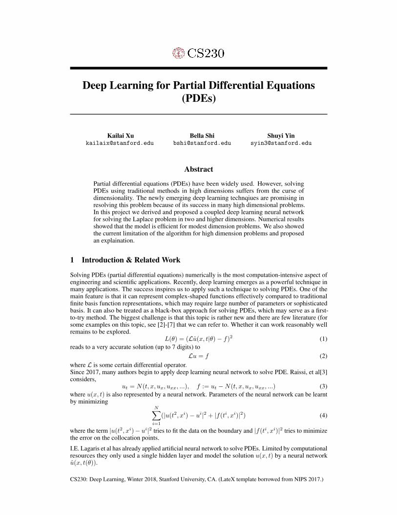
The data set is generated randomly both on the boundaries and in the innerdomain. For every updatein Line 3, we randomly generate (xi, yi)Mi=1, (xi, yi) ∈ ∂Ω and compute gi = gD(xi, yi). Thedata are then fed to (2) for computing loss and derivatives.

For every update in Line 4, we randomly generate (xi, yi)Ni=1, (xi, yi) ∈ Ω and compute fi =f(xi, yi). The data are then fed to (1) for computing loss and derivatives.

Figure 1: Data Generation for Training the Neural Network. We sample randomly from the innerdomain Ω and its boundary ∂Ω. Here × represents the sampling points within the domain and represents the sampling points on the boundary.

3 Approach

Our main focus is elliptic PDEs, which is generally presented as:

− ∂

∂x

(p(x, y)

∂u

∂x

)−− ∂

∂y

(q(x, y)

∂u

∂y

)+ r(x, y)u = f(x, y), in Ω

u = gD(x, y), on ΩD

p(x, y)∂u

∂x

∂y

∂s− q(x, y)

∂u

∂y

∂x

∂s+ c(x, y)u = gN (x, y), on ΩN

(5)

In the case p = q ≡ −1, r ≡ 0, ∂ΩD = ∂Ω, we obtain the Poisson equation:4u = f, in Ω

u = gD on ∂Ω(6)

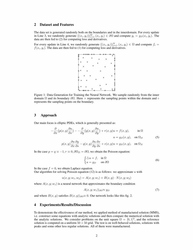
In the case f = 0, we obtain Laplace equation.Our algorithm for solving Poisson equation (12) is as follows: we approximate u with

u(x, y;w1, w2) = A(x, y;w1) +B(x, y) ·N(x, y;w2)

where A(x, y;w1) is a neural network that approximates the boundary condition

A(x, y;w1)|∂Ω≈ gD (7)

and where B(x, y) satisfies B(x, y)|∂Ω≡ 0. Our network looks like this fig. 2.

4 Experiments/Results/Discussion

To demonstrate the effectiveness of our method, we applied method of manufactured solution (MMS),i.e. construct some equations with analytic solutions and then compare the numerical solution withthe analytic solutions. We consider problems on the unit square Ω = [0, 1]2, and the referencesolution is computed on a uniform 50× 50 grid. The test is on well-behaved solutions, solutions withpeaks and some other less regular solutions. All of them were manufactured.

2

Figure 2: The structure of our network. We proposed this idea at the inspiration of GAN, where weupdate the boundary network for several times before we update the PDE network once. Our lossfunction is made up of two components: boundary loss and interior loss.

4.1 Example 1: Well-behaved Solution

Consider the analytical solution

u(x, y) = sinπx sinπy, (x, y) ∈ [0, 1]2 (8)

then we havef(x, y) = ∆u(x, y) = −2π2 sinπx sinπy (9)

and the boundary condition is zero boundary condition.

The hyper-parameters for the network include ε = 10−5, L = 3, n[1] = n[2] = n[3] = 64. Infigures below, the red profile shows exact solutions while the green profile shows the neural networkapproximation. Figure 3 (a) shows the initial profiles of the neural network approximation, whilefig. 3 (c) shows that after 300 iterations it is nearly impossible to distinguish the exact solution andthe numerical approximation.

(a) (b) (c)

Figure 3: Evolution of the neural network approximation. At 300 iteration, it is hard to distinguishnumerical solution and exact solution by eyes.

3

(a) (b) (c)

Figure 4: Loss and error of the neural network. For Lb, we have adopted an early termination strategyand therefore the error stays around 10−5 once it reaches the threshold. The PDE error Li and L2

error approximation keeps decreasing, indicating effectiveness of the algorithm.

4.2 Example 2: Solutions with a Peak

Consider the manufactured solution

u(x, y) = exp[−1000(x− 0.5)2 − 1000(y − 0.5)2] + v(x, y) (10)

where v(x, y) is a well-behaved solution, such as the one in section 4.1. Figure 5 shows the plotof exp[−1000(x− 0.5)2 − 1000(y − 0.5)2]. We classify this kind of function as ’ill-behaved’ dueto its dramatical change at a small area and therefore leads to very large Laplacian. This can bedifficult for the neural network approximation to work. The gradient of the optimizer can be verylarge and a general step size will take the solution to badly behaved ones. As an illustration, letv(x, y) = sin(πx). If we do not do the singularity subtraction and run the neural network programdirectly, we obtain fig. 5. We see that the numerical solution diverges.

(a) (b) (c)

Figure 5: Plot of exp[−1000(x− 0.5)2 − 1000(y − 0.5)2], which has a peak at (0.5, 0.5), and theevolution across iterations. This extreme behavior proposes difficulty for neural network approxi-mation, since the Laplacian around (0.5, 0.5) changes dramatically and can be very large. Solutionconverges on the boundary after several iterations but because of the peak, it diverges within thedomain.

4.3 Example 3: Less Regular Solutions

Consider the following manufactured solution

u(x, y) = y0.6 (11)

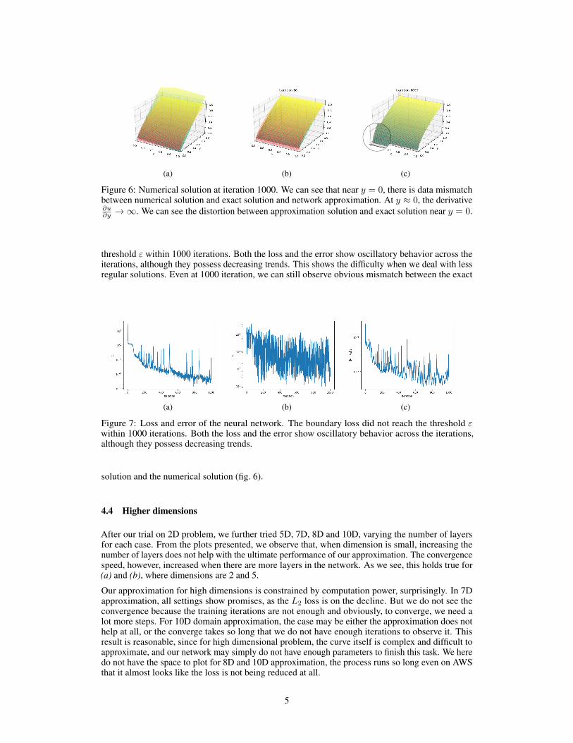
the derivative of the solution goes to infinity as y → ∞, which makes the loss function hard tooptimize. In the meanwhile, we notice that for any interval [δ, 1], δ > 0, the derivatives of u(x, y) on[0, 1]×[δ, 1] is bounded, that is to say, only the derivatives near y = 0 bring trouble to the optimization.Figure fig. 6 shows the initial profile of the neural network approximation. See Section 4.1 for detaileddescription of the surface and notation. The convergence is less satisfactory than section 4.1. Figure 8shows the loss and error plot with respect to training iterations. The boundary loss did not reach the

4

(a) (b) (c)

Figure 6: Numerical solution at iteration 1000. We can see that near y = 0, there is data mismatchbetween numerical solution and exact solution and network approximation. At y ≈ 0, the derivative∂u∂y →∞. We can see the distortion between approximation solution and exact solution near y = 0.

threshold ε within 1000 iterations. Both the loss and the error show oscillatory behavior across theiterations, although they possess decreasing trends. This shows the difficulty when we deal with lessregular solutions. Even at 1000 iteration, we can still observe obvious mismatch between the exact

(a) (b) (c)

Figure 7: Loss and error of the neural network. The boundary loss did not reach the threshold εwithin 1000 iterations. Both the loss and the error show oscillatory behavior across the iterations,although they possess decreasing trends.

solution and the numerical solution (fig. 6).

4.4 Higher dimensions

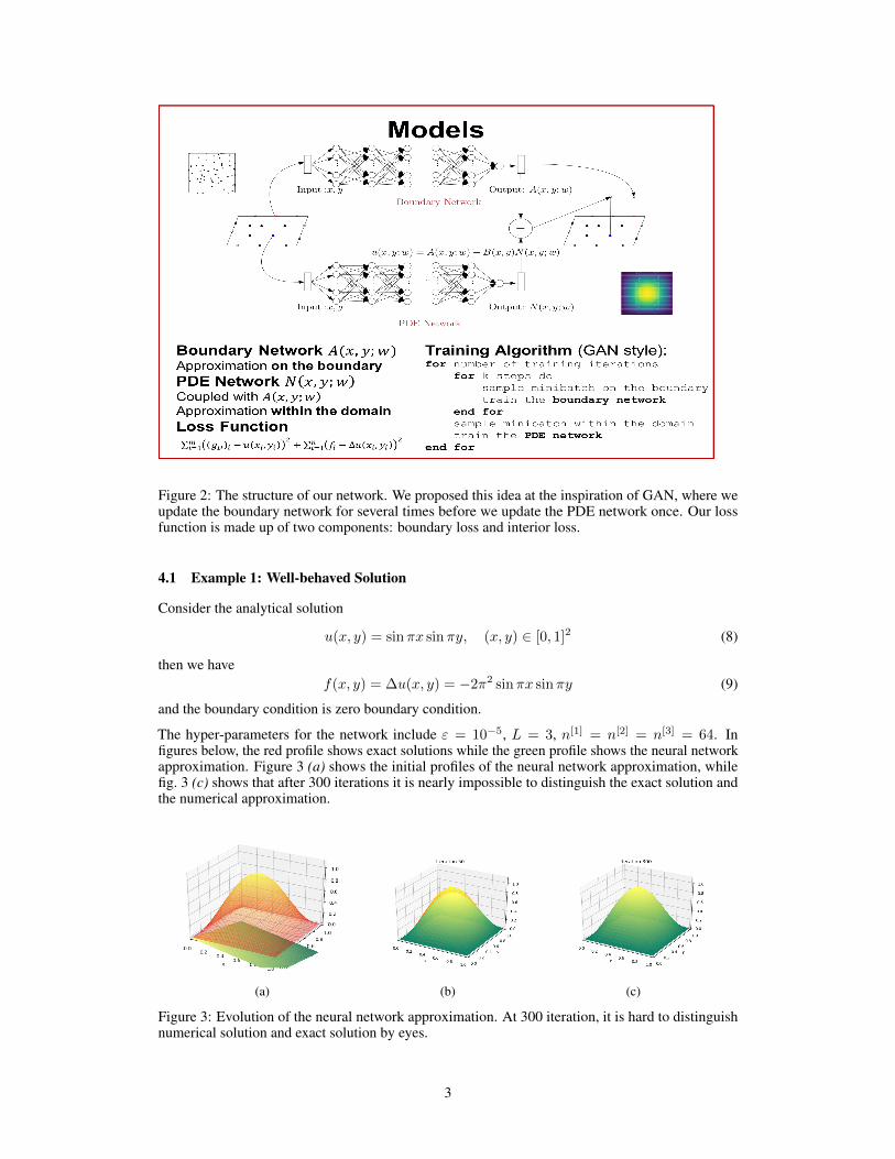
After our trial on 2D problem, we further tried 5D, 7D, 8D and 10D, varying the number of layersfor each case. From the plots presented, we observe that, when dimension is small, increasing thenumber of layers does not help with the ultimate performance of our approximation. The convergencespeed, however, increased when there are more layers in the network. As we see, this holds true for(a) and (b), where dimensions are 2 and 5.

Our approximation for high dimensions is constrained by computation power, surprisingly. In 7Dapproximation, all settings show promises, as the L2 loss is on the decline. But we do not see theconvergence because the training iterations are not enough and obviously, to converge, we need alot more steps. For 10D domain approximation, the case may be either the approximation does nothelp at all, or the converge takes so long that we do not have enough iterations to observe it. Thisresult is reasonable, since for high dimensional problem, the curve itself is complex and difficult toapproximate, and our network may simply do not have enough parameters to finish this task. We heredo not have the space to plot for 8D and 10D approximation, the process runs so long even on AWSthat it almost looks like the loss is not being reduced at all.

5

(a) (b) (c)

Figure 8: Performance of approximation for domains in different dimensions. In low dimensionalproblems, we see the convergence fast, and the more layers we have in the neural network, the fasterconvergence we observe; the number of layers do not affect the ultimate performance, measuredin L2 loss. The higher the dimensions are, the more difficult for us to see convergence, or in otherwords, the more iterations the approximation requires to achieve convergence. Notice in (c), for 7Ddomain approximation, we cannot see the convergence in 30K iterations, but in general the loss isbeing reduced.

5 Conclusion/Future Work

In this project, we proposed novel deep learning approaches to solve the Lapalce equation,4u = f, in Ω

u = gD on ∂Ω(12)

We also showed results for different kinds of solutions, and discussed the high dimension cases aswell.In the future, we will generalize results to other types of PDEs, and also investigate algorithms forill-behaved solutions, such as peaks, exploding gradients, oscillations, etc.

6 Contributions

Kailai worked on mathematical formulation of the methods, while Bella and Shuyi worked on themodel tuning and realization. The source code can be seen at https://github.com/kailaix/nnpde.

References

[1] Wang, Zixuan, et al. Sparse grid discontinuous Galerkin methods for high-dimensional elliptic equations.Journal of Computational Physics 314 (2016): 244-263.

[2] I.E. Lagaris, A. Likas and D.I. Fotiadis. Artificial Neural Networks for Solving Ordinary and PartialDifferential Equations, 1997.

[3] Maziar Raissi. Deep Hidden Physics Models, Deep Learning of Nonlinear Partial Differential Equations,2018.

[4] Justin Sirignano and Konstantinos Spiliopoulos. DGM: A deep learning algorithm for solving partialdifferential equations, 2007.

[5] Weinan E, Jiequn Han, and Arnulf Jentzen. Deep learning-based numerical methods for high-dimensionalparabolic partial differential equations and backward stochastic differential equations, 2017.

[6] Zichao Long, Yiping Lu, Xianzhong Ma, and Bin Dong. PDE-Net, Learning PDEs from data, 2018.

[7] Modjtaba Baymani, Asghar Kerayechian, Sohrab Effati. Artificial Neural Networks Approach for SolvingStokes Problem, Applied Mathematics 2010.

[8] M.M. Chiaramonte and M. Kiener. Solving differential equations using neural networks.

[9] Peng, Shige, and Falei Wang. BSDE, path-dependent PDE and nonlinear Feynman-Kac formula. ScienceChina Mathematics 59.1 (2016): 19-36.

6