Deferred Maintenance of Disk-Based Random Samples

Deferred Maintenance of Disk-Based RandomSamples

Rainer Gemulla and Wolfgang Lehner

Dresden University of Technology, 01099 Dresden, Germany{gemulla, lehner}@inf.tu-dresden.de

Abstract. Random sampling is a well-known technique for approximateprocessing of large datasets. We introduce a set of algorithms for incre-mental maintenance of large random samples on secondary storage. Weshow that the sample maintenance cost can be reduced by refreshing thesample in a deferred manner. We introduce a novel type of log file whichfollows the intuition that only a “sample” of the operations on the basedata has to be considered to maintain a random sample in a statisticallycorrect way. Additionally, we develop a deferred refresh algorithm whichupdates the sample by using fast sequential disk access only, and whichdoes not require any main memory. We conducted an extensive set ofexperiments and found, that our algorithms reduce maintenance cost byseveral orders of magnitude.

1 Introduction

Random samples are widely used as versatile synopses for large datasets. Suchsynopses are a must or at least desirable in most real-world scenarios. On theone hand, the complete dataset may not be accessible. For example, the datasetproduced by a data stream is unbounded in size, and it is often too expensiveto keep track of all the data elements which ever entered the system. Thus, asynopsis with a bounded size, i.e., independent of the dataset size, allows forinference of statistical properties of the dataset at the cost of some precision. Onthe other hand, the effort to process the complete dataset may be unacceptablyhigh, e.g., when the dataset is very large or when the complexity of the algorithmsexceeds the available resources. The latter case is ubiquitous in data warehousesystems which typically contain a huge amount of data subject to complex datamining algorithms.

Within the last decade, random sampling has been proposed as an adequatetechnique to summarize large datasets. Most applications require uniform sam-ples to derive precise results and error bounds, i.e., each sample of the same sizeis equally likely to be produced. There exists a variety of alternative synopsesfor certain scenarios, but uniform random sampling bears the advantage of ap-plication neutrality. Whenever it is not known in advance which estimates willbe computed on the synopsis, a uniform random sample is a good choice.

Random samples may be computed on-the-fly in certain scenarios. However,this is typically expensive—if not impossible—to perform [1]. Alternatively, one

Y. Ioannidis et al. (Eds.): EDBT 2006, LNCS 3896, pp. 423–441, 2006.c© Springer-Verlag Berlin Heidelberg 2006

424 R. Gemulla and W. Lehner

may materialize the sample and update it if the underlying dataset changes. Sincesynopsis maintenance is no “free” operation, i.e., it has a performance impact onthe processing of updates to the dataset, the cost for maintenance should be assmall as possible. In the database community, research has shown that it is moreefficient to decouple the update of a materialized view from operations on theunderlying dataset [2]. This approach is typically referred to as deferred refresh.Contributions. In this paper, we propose deferred maintenance strategies fordisk-based random samples with a bounded size. Our approach is based on thewell-known reservoir sampling scheme. We introduce a novel type of log file andshow that it is sufficient to keep track of only a “sample” of the operations onthe dataset to maintain a statistically correct random sample. Furthermore, wedevelop an algorithm for deferred refresh, which performs only fast sequentialI/O operations, minimizes the number of reads and writes to the sample, anddoes not require any main memory. Our experiments indicate, that deferredmaintenance reduces the maintenance cost by several orders of magnitude.Assumptions. We assume that the random sample is too large to fit into themain memory and thereby resides on secondary storage. In fact, many estimatorsbased on samples require the sample to be sufficiently large, e.g., even “simple”statistics estimators like the estimation of the number of distinct values do notperform well on undersized samples. The situation gets worse if more complexalgorithms are executed on the sample, e.g., association rule mining or cluster-ing algorithms. Moreover, the overall memory consumption increases with thenumber of samples maintained in-memory.

Concerning the storage system, we assume that sequential access is faster thanrandom access, and that the storage system tries to store data in a sequentialsequence of blocks.1 For example, if the data is stored on a hard disk, sequentialaccess is indeed faster than random access. Most file systems try to arrange datain sequential blocks to make use of this fact, and file system caches allow for“conversion” of random (write) accesses to sequential ones. Again, we assumethat the sample is large, and therefore, the effectiveness of the cache is limited.

Throughout the paper, we assume that access to the base data is disallowed atany time. The sample maintenance algorithms “see” only the insertions, updatesand deletions executed on the underlying dataset. The internal structure of thedataset is of no interest to the sampling algorithm, so that our approach nativelyextends to arbitrary settings, e.g., data streams, SQL views or XML reposi-tories. We subsequently assume that the random sample is computed from adataset R.

Paper Organization. The remainder of the paper is structured as follows: InSection 2, we discuss related work from the sampling, database and data streamcommunity. Section 3 introduces a novel logging scheme which minimizes storageconsumption and logging overhead. In Section 4, we propose efficient algorithms

1 Even if sequential and random access perform similarly, our algorithms reduce thetotal number of accesses to the storage system. Moreover, if the storage system doesnot align data in blocks, the performance of our algorithms increases.

Deferred Maintenance of Disk-Based Random Samples 425

to refresh the sample by accessing the log file only. In Section 5 we discuss theapplicability of our algorithms in the environment of a DBMS. An extensive setof experiments is presented in Section 6. We conclude the paper with Section 7.

2 Related Work

We first present general techniques for bounded-size random sampling, and thendiscuss specific methods for sampling in a data stream system as well as in adatabase system.

Uniform sampling. Bounded-size sampling schemes produce uniform samplesof a given size M . Sequential sampling [3] is one of the most efficient samplingschemes which fall into this category. It accesses exactly M elements of R tocompute the sample. Unfortunately, sequential sampling has to know the datasetsize in advance, thus, it is not applicable to sample maintenance. However, thewell-known reservoir sampling scheme [4] is able to maintain a sample of adataset of unknown size, as long as there are only insertions. The basic idea isto insert the first M elements into the sample. Afterwards, each newly arrivingelement replaces a random element of the sample with probability M/(|R|+1), oris rejected otherwise. Vitter [4] developed some techniques to efficiently computethe next element to be inserted into the sample. All the algorithms presented inthis paper are based on reservoir sampling.

Sampling data streams. Sampling is ubiquitous in data stream managementsystems for the following two reasons: On the one hand, sampling is used tocope with high system load. If the number of arriving elements is too high tobe processed completely, one may “simply” throw away some of the streamelements. This approach often appears in the context of load shedding [5, 6]. Onthe other hand, inference of statistical properties for the whole data stream seenso far is challenging since complete materialization of the stream is not feasible.One solution to this problem is the maintenance of a random sample of thecomplete data stream, potentially with some bias towards newer elements [7].The maintenance algorithm has to be efficient, so that it can deal with the higharrival rates found in typical data stream scenarios.

Jermaine et al. introduced the geometric file (GF) [7], a technique for disk-based maintenance of samples from a data stream. The technique is based onreservoir sampling and minimizes I/O efforts by decreasing the number of ac-cessed blocks. In fact, the major part of the GF is never read, most updates haveblock-level granularity and are written sequentially. However, the GF makes useof an in-memory buffer, and its performance depends strongly on the size of thisbuffer. Since each maintained sample requires its own buffer, the GF does notscale well with the number of samples. The GF is a deferred refresh algorithmsince the sample is updated only if the buffer is completely filled. We comparethe GF with our algorithms in Section 6.5.Sampling in databases. Database samples are often tailored to their appli-cation, e.g., to represent a given workload [8], to handle data skew [9] or to


support joins [10] and groupings [11, 12]. Most of these techniques make use ofrandom sampling and extend it by some means or other [7, 8, 9, 10, 11, 12, 13]. Infact, there are lots of sampling schemes which rely on reservoir sampling. Thesealgorithms can be natively extended to support fast deferred refresh using thetechniques presented in this paper. We discuss issues specific to database systemsin Section 5.

3 Logging and Refresh

In this paper, we consider the maintenance of a random sample computed froma dataset R. In the following, we assume that a uniform random sample of sizeM has been computed already (e.g., using reservoir sampling), and that thissample is maintained as the underlying data changes. We distinguish immediaterefresh strategies, which always keep the sample up-to-date, and deferred refreshstrategies, which refresh the sample from time to time (e.g., lazily or periodically,see [2]). We say that a maintenance strategy is incremental if it never accessesthe base data directly, but only the elements which are inserted.2

Incremental maintenance strategies consist of two phases: A log phase cap-tures the insertions into the dataset, and a refresh phase updates the sampleusing the logged data. This holds for both immediate and deferred refresh strate-gies. In fact, immediate refresh can be seen as a deferred maintenance strategywhich refreshes the sample every time the log has changed. In this section, weintroduce several strategies for realizing the log phase in the case of randomsampling. We assume that the log file resides on secondary storage, so that nomemory is consumed. Additionally, we present naive refresh algorithms whichupdate the sample using the log file.

3.1 Full Logging

The most basic logging strategy is to write all the insertions into the log file. Werefer to this approach as full logging. Probably the simplest way to refresh thesample using the full log is to apply reservoir sampling subsequently to each ofits elements. We denote this approach naive full refresh. Clearly, this strategydoes not make use of the fact that the log file may contain more informationthan needed to update a sample, since the sample itself reflects only a portionof the underlying dataset. As will become evident in Section 5, there are moreefficient refresh strategies with full logs.

The example in Figure 1 depicts a sample consisting of five elements andthe full log file after 45 elements have been inserted. The reservoir samplingalgorithm decides for every element whether it is included in the sample or not.In the former case, the element is called a candidate and replaces a randomelement of the sample. In the latter case, the element is ignored. As we proceedthrough the log, there are more and more candidates selected, and each of these2 We preliminarily assume that the dataset is subject to insertions only, and extend

our results to updates and deletions in Section 5.


Fig. 1. Deferred sample maintenance using a full log

candidates can potentially overwrite a candidate (within the sample) which hasbeen written earlier during the refresh phase. We say that a candidate is final ifit is not overwritten within the current refresh operation.

Clearly, the above approach has serious disadvantages:

1. Obviously, most of the elements in the full log are not accepted into thesample and therefore logged unnecessarily. In the example, 11 out of 45elements are made candidates, while only 4 of them remain in the finalsample.

2. Updating the sample relies on random I/O (though the logfile is read se-quentially). This property is directly inherited from the reservoir samplingalgorithm.

3. The algorithm performs unnecessary I/O operations since the non-final can-didates are overwritten by later candidates.

We propose an alternative refresh strategy for full logs in Section 5 whicheliminates (2) and (3) above.

3.2 Candidate Logging

The elimination of (1) above is straightforward. The basic idea is that the ele-ments which are ignored by the refresh operation do not have to be included inthe log file. Therefore, we push the acceptance test of the reservoir sampling al-gorithm to the log phase.3 Instead of logging every element added to the dataset,we decide on-the-fly whether the element is made a candidate or not. Thus, wewrite an arriving element to the log file with probability M/(|R|+1) or ignore itotherwise. We refer to this logging strategy as candidate logging and denote thelog file C = {c1, . . . , cl}. Note that the order of the elements within the log isimportant since each candidate has been accepted with a different probability.

For example, instead of writing all 45 elements of Figure 1 to the full log,we only need to log the 11 candidates shown in Figure 2. In fact, the smallerthe sample size with respect to the current dataset size, the more elements areskipped between two candidates on average. If we insert n elements into R, theexpected log file size is given by3 We are free to use any other acceptance test. For example, the biased reservoir

sampling scheme in [7] is more suitable for data stream sampling.


Fig. 2. Deferred sample maintenance using a candidate log

E(|C|) =n∑

i=1

M

|R| + i≈ M ln

|R| + n

|R| .

Here, we used the logarithmic approximation for harmonic numbers. Notethat E(|C|) decreases as |R| increases. The refresh algorithm has to be modifiedto make sure that every element of the candidate log is inserted into the sample.We scan the candidate log sequentially and write each candidate to a randomposition in the sample. We refer to this algorithm as naive candidate refresh. Itsequentially reads |C| elements of the log file and randomly writes |C| elementsto the sample.

Within the next section, we develop algorithms which reduce the number ofread and written elements, and access both the log file and the sample sequen-tially (thereby eliminating (2) and (3) above).

4 Algorithms for Candidate Refresh

The naive candidate refresh algorithm has the undesirable property that accessto the sample is non-sequential. Additionally, candidates written to the samplemay be overwritten by subsequent candidates. This is clearly inefficient sinceit suffices to write out only the last candidate assigned to each element of thesample. The easiest way to circumvent these drawbacks is to precompute thechanges to the sample and to write out the final candidates afterwards. Thus, allthe algorithms presented in this section consist of a precomputation phase anda write phase. Using this approach, we can avoid random I/O completely whileat the same time reducing the total number of disk accesses. We will presentthree different algorithms for precomputation, one using an in-memory array,one using an in-memory LIFO-stack, and one using no memory at all.

4.1 Array Refresh

Let A be an integer array of size M with all of its elements set to empty. We canuse A to determine which elements of the candidate log are going to be includedin the final sample. We modify the naive refresh algorithm as follows: Instead ofphysically reading the candidate log C = {c1, . . . , cl}, we operate on the indexes1, . . . , l of the candidates within the log and thereby preliminarily avoid access


Fig. 3. Array Refresh

Algorithm 1. Array RefreshRequire: sample size M , candidate log C1: create an in-memory array A with M empty elements2: for i = 1 to |C| do // indexes of the candidates3: write i to a random element of A4: end for5: sort non-empty fields of A // optional6: for j = 1 to M do // indexes of the sample7: if A[j] is not empty then8: read candidate A[j]9: write candidate to the jth element of the sample

10: end if11: end for

to the log file. Furthermore, instead of writing the candidates to the sample,we store their indexes in the respective element of the in-memory array A. Thisprevents the random I/O of the naive algorithm.

Array A is shown for the example data in Figure 3. For clarity, empty fieldsare striped and indexes are written in italic and bold letters. The array consistsof some empty elements and some elements containing indexes. This informa-tion is sufficient to refresh the sample in a sequential scan. Let j = 1, . . . ,Mdenote the current position within the sample. We look up the jth value in A(denoted A[j]) and check whether it contains an index or not. In the formercase, we write the candidate with the index A[j] to the current element of thesample. We refer to sample elements which are overwritten during the refreshas displaced elements. In the latter case, A[j] is empty and we leave the cur-rent element of the sample as it is (we do not read it actually). These elementsare denoted stable. Note that we do not know which elements of the sampleare stable and which are displaced until we have finished the precomputationphase.

The Array Refresh algorithm is summarized in Algorithm 1, and an exampleis shown in Figure 3. Access to the sample is now sequential, but access to thelog file is not. However, since the order of the elements within the sample isof no interest, we may sort array A right after the preprocessing phase. Care


must be taken that the sort algorithm does not move empty elements to anotherposition. These elements are linked with stable elements which in turn should bedistributed randomly. Using the sorted array, access to the log file is sequential.

To analyze the I/O effort of the Array Refresh algorithm, we define a randomvariable Ψj which evaluates to 1 if the jth element of the sample is displaced andto 0 otherwise (1 ≤ j ≤ M). Clearly, the probability that an element is displacedis independent of its position within the sample:

P (Ψj = 1) = 1 −(

1 − 1M

)|C|

In the example, each element is displaced with a probability of roughly 91%.Let Ψ =

∑Ψj describe the total number of displaced elements, which corre-

sponds to the number of elements read from the candidate log and subsequentlywritten to the sample. By linearity of the expected value we get

E(Ψ) = M

(1 −

(1 − 1

M

)|C|)

This evaluates to 4.57 in the example (Ψ itself equals 4). The Array Refreshalgorithm performs Ψ sequential reads from the log file and Ψ sequential writesto the sample with Ψ ≤ min(M, |C|). Therefore, Array Refresh performs betterthan the naive refresh algorithm. However, array A consumes a lot of memoryand sorting A is an expensive operation. The next algorithm reduces the memoryconsumption from M to Ψ indexes and does not require a sort operation.

4.2 Stack Refresh

The Stack Refresh algorithm is based on the observation that the probabilityof overwriting a candidate by subsequent candidates is decreasing during theprocessing of the candidate log. For example, the first candidate may be over-written by all the other candidates, while the last one is never overwritten.Again, we precompute the indexes of the candidates which are going to be writ-ten to the sample. A stack is used as internal data structure in order to avoidsorting.

The candidate indexes are processed in reverse order, that is, from |C| to 1.For each index i, we decide whether it is part of the sample or overwritten by oneof the indexes already processed. The latter is the case if i falls onto a positionin the sample which is already occupied by one of the candidates. For example,suppose we process the candidate log as shown in Figure 3 but in reverse order.Candidate index 11 occupies sample position 1. Therefore, candidate indexes9 and 3 – which also try to occupy position 1 – are both overwritten by 11.Therefore, only 11, 10, 8 and 6 are final in the example.

During the precomputation phase, each index i is selected with probabilitypk = (M −k)/M with k being the number of indexes selected already. Obviously,pk remains constant as long as no index selected. The random variable Xk


Fig. 4. Stack Refresh

describes how many indexes we have to skip until the next one is selected. Xk

is geometrically distributed:

P (Xk = x) = P (skip x elements, select (x + 1)th element)

= (1 − pk)xpk =(

k

M

)x (M − k

M

)

To summarize: We select the first index |C|. Afterwards, we generate X1, skipX1 indexes, and select the next one. This process is repeated using X2, X3, andso on. The algorithm stops as soon as M indexes have been selected or if thereare no more candidates (i < 1). As can be seen in Figure 4, the indexes areselected in descending order. Therefore, we use a LIFO-stack to keep track ofthe selected indexes and to reverse their order.

In contrast to the Array Refresh algorithm, we do not maintain the infor-mation on which index falls onto which position. In other words, we do notprecompute the set of stable and displaced elements. After the precomputationphase has finished, the stack only contains the indexes of the candidates whichhave to be written to the sample. We have to decide which of the correspond-ing candidates have to be written to which position of the sample, and whichelements of the sample remain stable.

If the stack contains k indexes and the sample has size M , there are M − kstable elements. In the example, the 4 selected indexes have to be distributedamong the 5 elements of the sample. Therefore, only a single element remainsstable. To refresh the sample, we scan it sequentially and decide for each positionwhether it remains stable or is overwritten by a candidate from the stack.4 Letj = 1, ...,M be the current position within the sample and k be the current stacksize. Then, position j is overwritten with probability:

qj,k =k

M − j + 1=

remaining indexesremaining sample elements

In summary, with probability qj,k we pop the uppermost index from the stack,read the corresponding candidate from the log file, and write it to the current4 This can be done efficiently using the sequential sampling scheme introduced in [3].


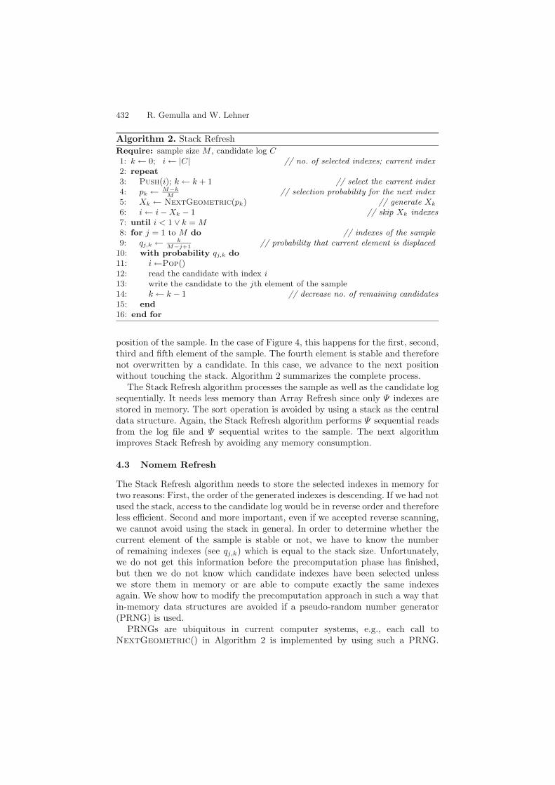
Algorithm 2. Stack RefreshRequire: sample size M , candidate log C1: k ← 0; i ← |C| // no. of selected indexes; current index2: repeat3: Push(i); k ← k + 1 // select the current index4: pk ← M−k

M// selection probability for the next index

5: Xk ← NextGeometric(pk) // generate Xk

6: i ← i − Xk − 1 // skip Xk indexes7: until i < 1 ∨ k = M8: for j = 1 to M do // indexes of the sample9: qj,k ← k

M−j+1 // probability that current element is displaced10: with probability qj,k do11: i ←Pop()12: read the candidate with index i13: write the candidate to the jth element of the sample14: k ← k − 1 // decrease no. of remaining candidates15: end16: end for

position of the sample. In the case of Figure 4, this happens for the first, second,third and fifth element of the sample. The fourth element is stable and thereforenot overwritten by a candidate. In this case, we advance to the next positionwithout touching the stack. Algorithm 2 summarizes the complete process.

The Stack Refresh algorithm processes the sample as well as the candidate logsequentially. It needs less memory than Array Refresh since only Ψ indexes arestored in memory. The sort operation is avoided by using a stack as the centraldata structure. Again, the Stack Refresh algorithm performs Ψ sequential readsfrom the log file and Ψ sequential writes to the sample. The next algorithmimproves Stack Refresh by avoiding any memory consumption.

4.3 Nomem Refresh

The Stack Refresh algorithm needs to store the selected indexes in memory fortwo reasons: First, the order of the generated indexes is descending. If we had notused the stack, access to the candidate log would be in reverse order and thereforeless efficient. Second and more important, even if we accepted reverse scanning,we cannot avoid using the stack in general. In order to determine whether thecurrent element of the sample is stable or not, we have to know the numberof remaining indexes (see qj,k) which is equal to the stack size. Unfortunately,we do not get this information before the precomputation phase has finished,but then we do not know which candidate indexes have been selected unlesswe store them in memory or are able to compute exactly the same indexesagain. We show how to modify the precomputation approach in such a way thatin-memory data structures are avoided if a pseudo-random number generator(PRNG) is used.

PRNGs are ubiquitous in current computer systems, e.g., each call toNextGeometric() in Algorithm 2 is implemented by using such a PRNG.


Algorithm 3. Nomem RefreshRequire: sample size M , candidate log C1: store state of the geometric PRNG2: compute X =

∑(Xk + 1) with k = M − 1, . . . , 1

3: restore state of the geometric PRNG4: i ← |C| − X // determine first index5: k ← M − 16: while i < 1 do // ignore negative indexes7: i ← i + Xk + 18: k ← k − 19: end while

10: for j = 1 to M do // indexes of the sample (k + 1 candidates left)11: with probability qj,k+1 = k+1

M−j+1 do // current element is displaced12: read the candidate with index i13: write the candidate to the jth element of the sample14: i ← i + Xk + 115: k ← k − 116: end17: end for

A PRNG computes a sequence of numbers which appears to be random. How-ever, the generated numbers depend only on an internal state. After a randomnumber has been computed, the PRNG advances to the next state by using acertain algorithm. This state transition is deterministic. The central idea of theNomem Refresh algorithm is to store the state of the PRNG before generatingthe sequence of selected indexes and to reset it afterwards to allow the genera-tion of the same sequence again. Therefore, there is no need to buffer the indexesin memory. The memory consumption of the PRNG state is negligible rangingfrom 1 to 1000 words for common generators [14].

Reconsider the random variable Xk of the Stack Refresh algorithm. It denoteshow many elements of the candidate log are skipped before the next one isselected. Since the Xk are independent of each other, it does not matter in whichorder they are generated. The Stack Refresh algorithm selects the candidateindexes in the following order (ignoring indexes smaller than 1):

|C|, |C| −1∑

k=1

(Xk + 1), |C| −2∑

k=1

(Xk + 1), . . . , |C| −M−1∑

k=1

(Xk + 1)

To generate this sequence in reverse order, we have to compute the quantityX =

∑M−1k=1 (Xk +1) to determine the first index (with k = M −1, . . . , 1). Then,

we subsequently add Xk + 1 to determine the next index. Therefore, each of theXk is accessed twice. As already stated, we avoid buffering of the Xk by resettingthe PRNG after the computation of X. The whole procedure is summarized inAlgorithm 3. For brevity, we omit details of the generation of Xk since it isidentical to Algorithm 2.

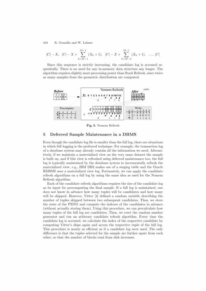
As illustrated in Figure 5, the Nomem Refresh algorithm selects the indexesin the following order (ignoring indexes smaller than 1):


|C| − X, |C| − X +M−1∑

k=M−1

(Xk + 1), |C| − X +M−1∑

k=M−2

(Xk + 1), . . . , |C|

Since this sequence is strictly increasing, the candidate log is accessed se-quentially. There is no need for any in-memory data structure any longer. Thealgorithm requires slightly more processing power than Stack Refresh, since twiceas many samples from the geometric distribution are computed.

Fig. 5. Nomem Refresh

5 Deferred Sample Maintenance in a DBMS

Even though the candidate log file is smaller than the full log, there are situationsin which full logging is the preferred technique. For example, the transaction logof a database system may already contain all the information we need. Alterna-tively, if we maintain a materialized view on the very same dataset the sampleis built on, and if this view is refreshed using deferred maintenance too, the fulllog is typically maintained by the database system to incrementally refresh thematerialized view, e.g., IBM DB2 makes use of a staging table and the OracleRDBMS uses a materialized view log. Fortunately, we can apply the candidaterefresh algorithms on a full log by using the same idea as used for the NomemRefresh algorithm.

Each of the candidate refresh algorithms requires the size of the candidate logas its input for precomputing the final sample. If a full log is maintained, onedoes not know in advance how many tuples will be candidates and how manywill be skipped. However, Vitter [4] defined a random variable describing thenumber of tuples skipped between two subsequent candidates. Thus, we storethe state of the PRNG and compute the indexes of the candidates in advance(without actually storing them). Using this procedure, we can precalculate howmany tuples of the full log are candidates. Then, we reset the random numbergenerator and run an arbitrary candidate refresh algorithm. Every time thecandidate log is accessed, we calculate the index of the respective candidate bycomputing Vitter’s skips again and access the respective tuple of the full log.This procedure is nearly as efficient as if a candidate log were used. The onlydifference is that the tuples selected for the sample are further apart from eachother, so that the number of blocks read from disk increases.


Another problem arising in the context of a DBMS is that there are updatesand deletions. We show how our refresh algorithms can be extended to supportthese operations as well. First, we store all updates in a separate log file andapply all these updates after each refresh of the sample. The situation becomesmore difficult if some elements are removed from the dataset. In this case, it is notpossible to maintain a candidate log since insertions after a deletion are includedin the sample with a different probability than assumed during candidate logging.Thus, we use a full log file if there are deletions. If we assume (or make sure)that the insertions and deletions are disjunctive, we first conduct all the deletionsand afterwards process the full log using the techniques presented in this paper(using a potentially smaller sample size). We currently investigate how a reservoirsample can be maintained so that deletions are supported as well.

6 Experiments

We implemented the various refresh algorithms and conducted a set of experi-ments to evaluate their performance. We distinguish between online, offline andtotal cost of maintaining the sample. The online cost is the processing cost of ar-riving insertions. The offline cost mirrors the cost for refreshing the sample. Thetotal cost is the sum of online and offline cost. This distinction is helpful sinceit captures different application areas. For example, in a streaming system, theonline cost is important since it expresses the processing time for each operationwithin the sample operator. The refresh may be conducted by an independentsystem which has access to the log file, thereby not affecting online processing.In a DBMS, both logging and refresh are typically conducted by the very samesystem, so that the total cost is more important than the online cost. For clarity,we arrange the figures for online and total cost side by side so that they can becompared easily. Note that most of the plots have logarithmic axes.Experimental results. We found that using a candidate log is significantlyfaster than refreshing the sample immediately or using a full log. When it comesto sample refresh, we found that the refresh algorithms using precomputationoutperform the naive ones, and that the computational overhead of Nomem Re-fresh is negligible. The more operations occur between two consecutive refreshoperations, the more is gained by using advanced refresh techniques. Our algo-rithms scale well, since the sample size has only a linear effect on the refreshcosts. In comparison to the geometric file, our techniques are more efficient if theGF is not allowed to consume large amounts of memory for its internal buffer.

6.1 Experimental Setup

The experiments were conducted on an Athlon AMD XP 3000+ system runningLinux with 2GB of main memory and an IDE hard drive with 7,200 RPM. Wefirst measured the access times per block using a 1.6GB on-disk sample (with acache of 100MB). Our hard disk is formatted with the ext3 filesystem. It has ablock size of 4096 bytes, and we assumed that each element occupies 32 bytes,


i.e., each block contains 128 elements. We found that a sequential read/writetakes about 0.094ms per block, a random read 8.45ms, and a random write5.50ms (due to asynchronous writes). Now, for each algorithm, we counted thenumber of sequential/random reads and writes on a block-level basis. We thenweighted these numbers with the access times above. This strategy allows forquantifying the cost of the single phases independently, while at the same timeenabling us to run a large variety of different experiments.

All the algorithms have been implemented using the Java programming lan-guage and Sun’s JDK version 1.5.0 03. For full refresh, we used the techniquesdescribed in Section 5. Unless stated otherwise, each experiment was run at leastone hundred times and results were averaged. We assumed that the sample isrefreshed periodically.

6.2 Online Cost

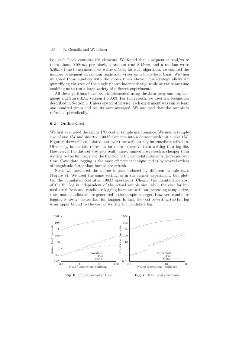
We first evaluated the online I/O cost of sample maintenance. We used a samplesize of one 1M and inserted 100M elements into a dataset with initial size 1M .Figure 6 shows the cumulated cost over time without any intermediate refreshes.Obviously, immediate refresh is far more expensive than writing to a log file.However, if the dataset size gets really large, immediate refresh is cheaper thanwriting to the full log, since the fraction of the candidate elements decreases overtime. Candidate logging is the most efficient technique and is by several ordersof magnitude faster than immediate refresh.

Next, we measured the online impact induced by different sample sizes(Figure 8). We used the same setting as in the former experiment, but plot-ted the cumulated cost after 100M operations. Clearly, the maintenance costof the full log is independent of the actual sample size, while the cost for im-mediate refresh and candidate logging increases with an increasing sample size,since more candidates are generated if the sample is larger. However, candidatelogging is always faster than full logging. In fact, the cost of writing the full logis an upper bound to the cost of writing the candidate log.

Cand.Full

ImmediateOnline

Cos

t(s

econ

ds)

No. of Operations (millions)1001010.1

100k

10k

1k

100

10

1

0.1

0.01

Fig. 6. Online cost over time

Cand.Full

ImmediateTot

alC

ost

(sec

onds)

No. of Operations (millions)1001010.1

100k

10k

1k

100

10

1

0.1

0.01

Fig. 7. Total cost over time


Cand.Full

Immediate

Online

Cos

t(s

econ

ds)

Sample Size (millions)10987654321

1M

100k

10k

1k

100

10

1

Fig. 8. Online cost and sample sizes

Cand.Full

ImmediateTot

alC

ost

(sec

onds)

Sample Size (millions)10987654321

1M

100k

10k

1k

100

10

1

Fig. 9. Total cost and sample sizes

Cand.Full

ImmediateOnline

Cos

t(s

econ

ds)

Refresh Period (thousands)100001000100101

100k

10k

1k

100

10

1

Fig. 10. Online cost and refresh period

Cand.Full

ImmediateTot

alC

ost

(sec

onds)

Refresh Period (thousands)100001000100101

100k

10k

1k

100

10

1

Fig. 11. Total cost and refresh period

Furthermore, we compared the online cost for different refresh periods(Figure 10). We used the same experimental setting as in the former experiments.The cost for maintaining the sample directly is independent of the refresh period(always 1). However, both candidate logging and full logging re-use the log fileafter a refresh so that one random I/O is performed to move from the currentposition to the beginning of the log file (otherwise, the costs are independent ofthe refresh period, too). Thus, with an increasing refresh period, these randomI/Os occur less frequently and the cost drops. Again, candidate logging is fasterthan full logging. Note that if the refresh period is less than 10k, the candidatelog often consists of only a single block, which is the minimum.

6.3 Total Cost

We ran the same experiments as above again but now measured the total I/Ocost (including refresh). Note that Array, Stack and Nomem Refresh have equalI/O cost. We refreshed the sample after every 1M insertions. As can be seen inFigure 7, deferred refresh is significantly faster than immediate refresh. The costsfor full and candidate refresh are almost the same since we used the algorithm


described in Section 5 for full refresh. However, the costs for writing the log fileare different, so that the candidate techniques are faster than the techniquesusing a full log. The I/O cost of the first few refreshes is magnified due to thelog-log-plot.

Figure 9 illustrates that the total costs for maintaining the sample are increas-ing as the sample size increases. Again, deferred refresh significantly outperformsimmediate refresh. The costs of full maintenance and candidate maintenance arealmost equal if the sample is really large. However, we performed 100 million op-erations in every case. If the number of operations were larger, this effect wouldvanish.

As can be seen in Figure 11, deferred refresh is faster than immediate refreshif refreshes are not extremely frequent. Since the total costs are governed by therefresh cost, full and candidate maintenance strategies perform equally if therefresh period is short. However, the larger the refresh period gets, the moreeffort is saved by using a candidate log. Thus, the candidate strategies becomemore efficient than full refresh in this case.

6.4 Memory Consumption and Computational Cost

In this experiment, we measured CPU cost and memory consumption for the dif-ferent implementations of deferred refresh. Even though the disk access patternis the same for Array, Stack and Nomem Refresh, their CPU and memory costsare different. For the experiments, we used a sample size of 1M elements. Weinserted elements until the number of candidates reached a certain size. Then,we refreshed the sample and measured the memory consumption and CPU cost.Note that computation and I/O are typically performed in parallel.

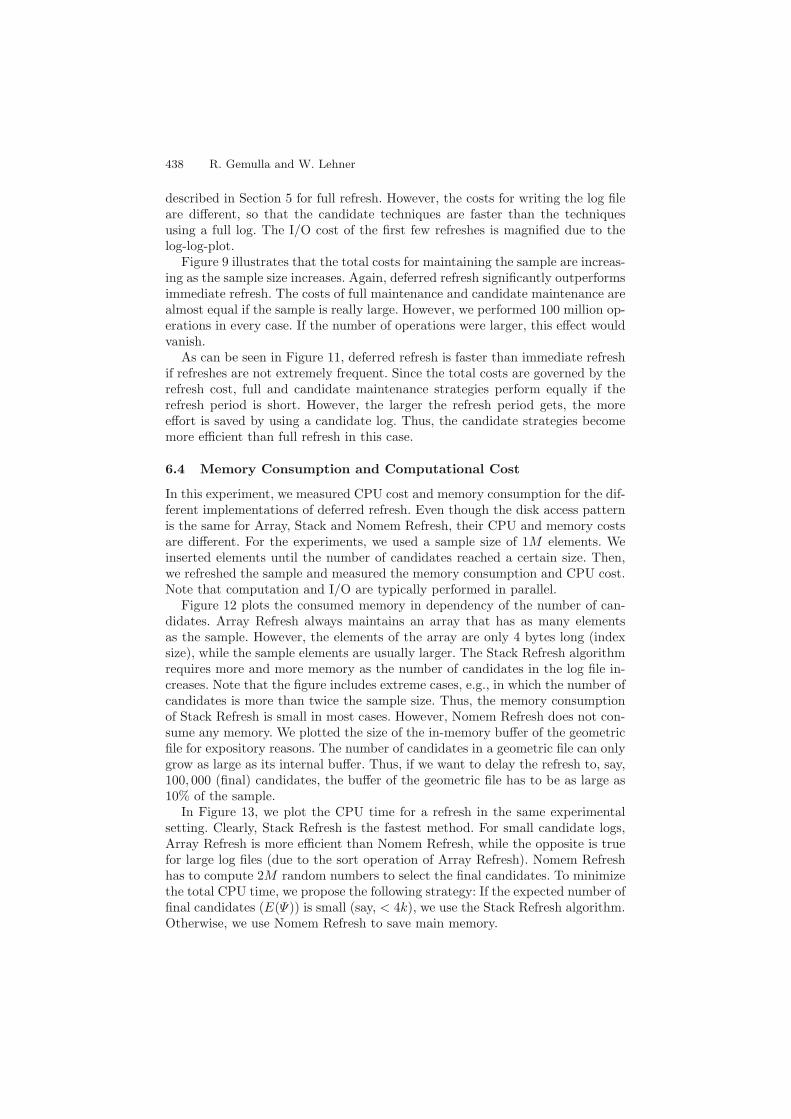
Figure 12 plots the consumed memory in dependency of the number of can-didates. Array Refresh always maintains an array that has as many elementsas the sample. However, the elements of the array are only 4 bytes long (indexsize), while the sample elements are usually larger. The Stack Refresh algorithmrequires more and more memory as the number of candidates in the log file in-creases. Note that the figure includes extreme cases, e.g., in which the number ofcandidates is more than twice the sample size. Thus, the memory consumptionof Stack Refresh is small in most cases. However, Nomem Refresh does not con-sume any memory. We plotted the size of the in-memory buffer of the geometricfile for expository reasons. The number of candidates in a geometric file can onlygrow as large as its internal buffer. Thus, if we want to delay the refresh to, say,100, 000 (final) candidates, the buffer of the geometric file has to be as large as10% of the sample.

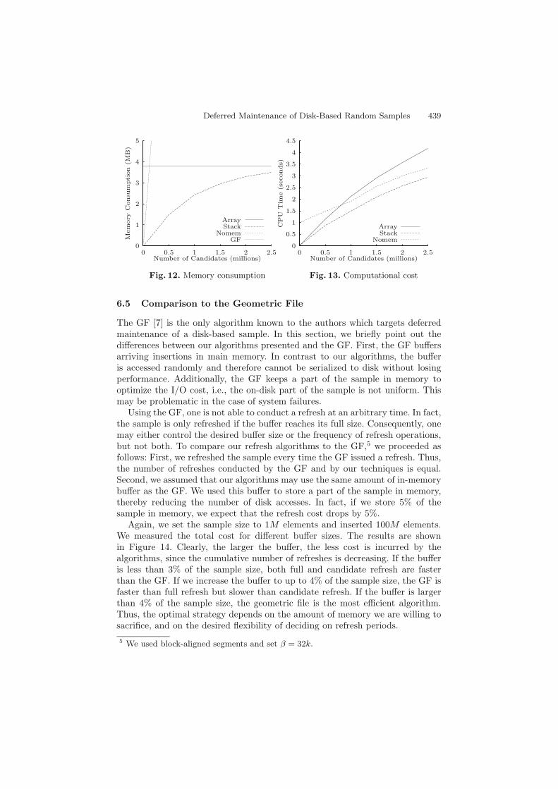
In Figure 13, we plot the CPU time for a refresh in the same experimentalsetting. Clearly, Stack Refresh is the fastest method. For small candidate logs,Array Refresh is more efficient than Nomem Refresh, while the opposite is truefor large log files (due to the sort operation of Array Refresh). Nomem Refreshhas to compute 2M random numbers to select the final candidates. To minimizethe total CPU time, we propose the following strategy: If the expected number offinal candidates (E(Ψ)) is small (say, < 4k), we use the Stack Refresh algorithm.Otherwise, we use Nomem Refresh to save main memory.


GFNomem

StackArray

Mem

ory

Con

sum

pti

on(M

B)

Number of Candidates (millions)2.521.510.50

5

4

3

2

1

0

Fig. 12. Memory consumption

NomemStackArrayC

PU

Tim

e(s

econ

ds)

Number of Candidates (millions)2.521.510.50

4.5

4

3.5

3

2.5

2

1.5

1

0.5

0

Fig. 13. Computational cost

6.5 Comparison to the Geometric File

The GF [7] is the only algorithm known to the authors which targets deferredmaintenance of a disk-based sample. In this section, we briefly point out thedifferences between our algorithms presented and the GF. First, the GF buffersarriving insertions in main memory. In contrast to our algorithms, the bufferis accessed randomly and therefore cannot be serialized to disk without losingperformance. Additionally, the GF keeps a part of the sample in memory tooptimize the I/O cost, i.e., the on-disk part of the sample is not uniform. Thismay be problematic in the case of system failures.

Using the GF, one is not able to conduct a refresh at an arbitrary time. In fact,the sample is only refreshed if the buffer reaches its full size. Consequently, onemay either control the desired buffer size or the frequency of refresh operations,but not both. To compare our refresh algorithms to the GF,5 we proceeded asfollows: First, we refreshed the sample every time the GF issued a refresh. Thus,the number of refreshes conducted by the GF and by our techniques is equal.Second, we assumed that our algorithms may use the same amount of in-memorybuffer as the GF. We used this buffer to store a part of the sample in memory,thereby reducing the number of disk accesses. In fact, if we store 5% of thesample in memory, we expect that the refresh cost drops by 5%.

Again, we set the sample size to 1M elements and inserted 100M elements.We measured the total cost for different buffer sizes. The results are shownin Figure 14. Clearly, the larger the buffer, the less cost is incurred by thealgorithms, since the cumulative number of refreshes is decreasing. If the bufferis less than 3% of the sample size, both full and candidate refresh are fasterthan the GF. If we increase the buffer to up to 4% of the sample size, the GF isfaster than full refresh but slower than candidate refresh. If the buffer is largerthan 4% of the sample size, the geometric file is the most efficient algorithm.Thus, the optimal strategy depends on the amount of memory we are willing tosacrifice, and on the desired flexibility of deciding on refresh periods.

5 We used block-aligned segments and set β = 32k.


GFCand.

FullImmediate

Tot

alC

ost

(sec

onds)

Buffer Fraction8%6%4%2%0%

100k

10k

1k

100

10

Fig. 14. GF buffer size & total cost

7 Summary

We developed a set of algorithms which allow for deferred maintenance of ran-dom samples of an arbitrary dataset. We introduced a novel type of log filewhich minimizes the amount of data used to track changes on the underlyingdataset. We showed that such a log file imposes far less overhead in processingarriving operations than traditional log files and immediate sample maintenance.Furthermore, we developed different strategies to efficiently process the log filein order to update the sample. We optimized our algorithms so that they relyon fast sequential disk access only, while the number of read and write oper-ations is minimized. Additionally, we showed how main memory consumptioncan be avoided at the cost of some CPU time. Finally, we conducted a set ofexperiments indicating that our algorithms are more efficient than any knownalgorithm using a small amount of in-memory data structures only.

Acknowledgement. This work has been supported by the German ResearchSociety (DFG) under LE 1416/3-1. We like to thank the anonymous reviewers,S. Schmidt, and P. Rosch for their helpful comments on a previous version ofthe paper.

References

1. Haas, P., Konig, C.: A Bi-Level Bernoulli Scheme for Database Sampling. In: Proc.ACM SIGMOD. (2004) 275–286

2. Gupta, A., Mumick, I.S., eds.: Materialized Views: Techniques, Implementations,and Applications. MIT Press (1999)

3. Vitter, J.S.: Faster Methods for Random Sampling. Commun. ACM 27 (1984)703–718

4. Vitter, J.S.: Random Sampling with a Reservoir. ACM TOMS 11 (1985) 37–575. Haas, P.J.: Data Stream Sampling: Basic Techniques and Results. In: Data Stream

Management: Processing High Speed Data Streams, Springer (2006) (to appear).


6. Tatbul, N., Cetintemel, U., Zdonik, S.B., Cherniack, M., Stonebraker, M.: LoadShedding in a Data Stream Manager. In: Proc. VLDB. (2003) 309–320

7. Jermaine, C., Pol, A., Arumugam, S.: Online Maintenance of Very Large RandomSamples. In: Proc. ACM SIGMOD. (2004) 299–310

8. Ganti, V., Lee, M.L., Ramakrishnan, R.: ICICLES: Self-Tuning Samples for Ap-proximate Query Answering. In: The VLDB Journal. (2000) 176–187

9. Chaudhuri, S., Das, G., Datar, M., Narasayya, R.M.V.R.: Overcoming Limitationsof Sampling for Aggregation Queries. In: Proc. ICDE. (2001) 534–544

10. Acharya, S., Gibbons, P.B., Poosala, V., Ramaswamy, S.: Join Synopses for Ap-proximate Query Answering. In: Proc. ACM SIGMOD. (1999) 275–286

11. Acharya, S., Gibbons, P.B., Poosala, V.: Congressional Samples for ApproximateAnswering of Group-By Queries. In: Proc. ACM SIGMOD. (2000) 487–498

12. Babcock, B., Chaudhuri, S., Das, G.: Dynamic Sample Selection for ApproximateQuery Processing. In: Proc. ACM SIGMOD. (2003) 539–550

13. Olken, F., Rotem, D.: Maintenance of Materialized Views of Sampling Queries.In: Proc. ICDE. (1992)

14. Matsumoto, M., Nishimura, T.: Mersenne Twister: A 623-Dimensionally Equidis-tributed Uniform Pseudo-Random Number Generator. ACM TOMACS 8 (1998)3–30

Date post:	12-Feb-2022
Category:	Documents
Upload:	others
View:	5 times
Download:	0 times

Deferred Maintenance of Disk-Based Random Samples

Documents