Degradation Modeling with Application-to Aging and ...

NUREG/CR-5612BNL-NUREG-52252

Degradation Modeling withApplication-to Aging andMaintenance EffectivenessEvaluations

Prepared byP. K} Samanta, W. E. Vesely, F. Hsu, M. Subudhi

Brookhaven National Laboratory

Science Applications International Corporation

Prepared forU.S. Nuclear Regulatory Commission

AVAILABILITY NOTICE

Availability of Reference Materials Cited In NRC Publcatlons

Most documents cited In NRC pubicatlons will be available from one of the following sources:

1. The NRC Public Document Room. 2120 L Street, NW, Lower Level, Washington, DC 20555

2. The Superintendent of Documents, U.S. Government Printing Office. P.O. Box 37082. Washington.DC 20013-7082

3. The National Technical Information Service. Springfield. VA 22181

Although the isting that follows represents the majority of documents cited In NRC publications, It Is notIntended to be exhaustive.

Referenced documents available for Inspection and copying for a fee from the NRC Public Document RoomInclude NRC correspondence and internal NRC memoranda; NRC Office of Inspection and Enforcementbulletins, circular*, Information notices, inspection and Investigatin notices: Ucensee Event Reports; ven-dor reports and correspondence; Commission papers; and applicant and licensee documents and corre-spondence.

The following documents In the NUREG series are available for purchase from the GPO Sales Program:formal NRC staff and contractor reports, NRC-sponsored conference proceedings. and NRC booklets andbrochures. Also available are Regulatory Guides, NRC regulations In the Code of Federal Regulations, andNuclear Regulatory Commission Issuances.

Documents avallable from the National Technical Information Service Include NUREG series reports andtechnical reports prepared by other federal agencies and reports prepared by the Atomic Energy Comnds-slon, forerunner agency to the Nuclear Regulatory Commisslon.

Documents available from pubic and special technical libraries Include all open literature Items, such asbooks, journal and periodical articles, and transactions. Federal Register notices, federal and state legisla-tion, and congressional reports can usually be obtained from these libraries.

Documents such as theses, dissertations, foreign reports and translations, and non-NRC conference pro-ceedings are available for purchase from the organization sponsoring the publication cited.

Single copies of NRC draft reports are avallable free, to the extent of supply, upon written request to theOffilce of Information Resources Management, Distribution Section, U.S. Nuclear Regulatory Commisslon.Washington, DC 20555.

Copies of Industry codes and standards used In a substantive manner In the NRC regulatory process aremaintained at the NRC Library. 7920 Norfolk Avenue, Bethesda, Maryland, and are availablo there for refer-ence use by the public. Codes and standards are usually copyrighted and may be purchased from theoriginating organization or, If they are American National Standards, from the American National StandardsInstitute, 1430 Broadway, New York. NY 10018.

DISCLAIMER NOTICE

This report was prepared as an account of wovrl sponsored by an agency of the United States GovernmentNeither the United States Government nor any agency thereof, orany of their errployeee, makes any warranty,expresed or Implied, or assumes any legal liability of responsibility for any third party's use, or the results ofsuch use, of any Information, apparatus, product or process disclosed In this report, or representsthat its useby such third party would not Infringe privately owned rights.

NUREG/CR-5612BNLNUREG-52252RV

Degradation Modeling withApplication to Aging andMaintenance EffectivenessEvaluations

Manuscript Completed. January 1991Date Published. March 1991

Prepared byP. K. Samanta, W. E. Vesely*, F. Hsu, M. Subudhi

S. K. Aggarwal, NRC Program Manager

Brookhaven National LaboratoryUpton, NY 11973

Prepared forDivision of Systems ResearchOffice of Nuclear Regulatory ResearchU.S. Nuclear Regulatory CommissionWashington, DC 20555NRC FIN A3270

OScience Applications International Corporation, Albuquerque, NM

ABSTRACT

This report describes a modeling approach to analyze component degradation andfailure data to understand the aging process of components. As used here, degradationmodeling is the analysis of information on component degradation in order to developmodels of the process and its implications. This particular modeling focuses on the analysisof the times of component degradations, to model how the rate of degradation changes withthe age of the component. The methodology presented also discusses the effectiveness ofmaintenance as applicable to aging evaluations.

The specific applications which are performed show quantitative models of componentdegradation rates and component failure rates from plant-specific data. The statisticaltechniques which were developed and applied allow aging trends to be effectively identifiedin the degradation data, and in the failure data. Initial estimates of the effectiveness ofmaintenance in limiting degradations from becoming failures also were developed. Theseresults are important first steps in degradation modeling, and show that degradation can bemodeled to identify aging trends.

i..

EXECUTIVE SUMMARY

The assessment of risk associated with aging in nuclear power plants encompassesmany facets, an important element of which is the understanding of the aging phenomenaassociated with components of safety systems. In this report, the aging phenomena at thecomponent level were studied to develop an aging reliability model representing the agingprocess experienced by components in nuclear power plants under presently existing test andmaintenance practices. A new model was developed to process information on componentdegradation in order to analyze the degradation process and its implications. The focus wason modeling the degradation rate, i.e., the rate at which degradations occur, and failure rate,i.e., the rate at which failures occur, with the specific objective of developing explicitrelationships between degradation characteristics and the component failure rate.

The research program goes beyond an analysis of times of degradation and failure.First, theoretical models that relate the degradation rate of the comnponent to its failure rateare developed. With the relationships derived, information on component degradation can beused to predict the component failure rate and its significance. Specifically, this methodol-ogy can use aging trends in the component degradation rate to predict future aging trends inthe component failure rate.

The capability of making such a prediction is important because the knowledge (orestimate) of related component aging failure rates is required to quantify the effects of agingon core damage frequency and risk. This knowledge is also needed to quantify theeffectiveness of a given maintenance program in controlling the effects of aging on the coredamage frequency and risk. However, failure data are often sparse. On the other hand,degradation data are more abundant because degradations occur at a higher rate than failures.Thus the methodology developed in this report allows component failure rates due to agingto be estimated from component degradation rates. This has the potential to greatly increasethe accuracy and availability of component aging failure rates made available to the user inrisk evaluations of aging effects.

It is important that, in addition to the identification of aging trends in degradation andfailure data, the methodology allows maintenance indicators to be selected in such a waythat component degradations are related to reliability and risk impacts. When the degradationindicators show significant impacts of degradation on the component failure rate and theresulting risk, maintenance should be performed to correct the degradations. Also, initialestimates of the effectiveness of maintenance in preventing degradations from becomingfailures were developed. Thus the degradation indicators can provide a practical andeffective means of monitoring component condition and signal for the correction ofdegradations before they have significant impacts on reliability and risk

The specific applications of the developed theoretical approach were performed, whichresulted in quantitative models of component degradation rates and component failure rates,all of them derived from plant-specific data. As part of the data analysis, statisticaltechniques that identify aging trends in failure and degradation data were developed. Theaging trends can be of any kind and can exist in any segment of the data. Specifically, ananalysis of residual heat removal (RHR) system pump data shows a wbathtub" curve for the

V

degradation rate where a distinct, increasing aging trend is observed as time progresses.Interestingly, the pump failure rate does not show any increasing trend for the same timeperiod, thus demonstrating the need to identify aging trends through analyses of componentdegradations.

In summary, these results reported are important first steps in showing that degradationscan be modeled to identify aging effects. The theoretical methodology that is developedrepresents an advancement, demonstrating that degradation characteristics are explicitlyrelated to failure-rate effects and hence ultimately to risk effects. Also, the effectiveness ofmaintenance can be analyzed and assessed. The next step would be to use the methodologyand statistical techniques to develop and validate practical procedures for predicting agingfailure rates from degradation data. This ability would provide powerful tools for analyzingaging effects in degradation data and for predicting their implications for reliability and risk.

vi

CONTENTS

ABSTRACT ........................................

EXECUTIVE SUMMRYY................................

LIST OF FIGURES .............-

ACKNOWvIEDGMENTS.................................

1. JRODUCION ...................................

2. CONCEPT AND OBJECTIVES OF DEGRADATION MODELING.....

3. METHODOLOGY: DEGRADATION MODELING APPROACHES ......3.1 State Representation of Degradation Modeling ................3.2 Transition Probabilities. .............................3.3 Degradation Frequency, Failure Frequency and Transition

Probabilities . .................. ...........3.4 Incorporation of Aging Effects in Degradation Moeling..........3.5 Aging Effect on Degradation Rate......................3.6 Basic Steps in Degradation Modeling .....................3.7 Assumptions and Limitations in the Methodology ..............

4. REGRESSION ANALYSIS USING COX'S MODEL TO ESTIMATEAGING RATES (DEGRADATION AND FAILURE RATES)..........

Page

iii

v

ix.

xi

1

3

S57

7S9

1010

4.1 Introduction....................................4.2 Cox's Model to Develop Aging Rates.....................4.3 The Regression Approach ............................

5. RESULTS AND INTERPRETATION OF AGE-RELATEDDEGRADA7ION AND FAILURE DATA.....................5.1 Analysis Approach................................5.2 AgingEffecton Degradation..........................5.3 AgingEffectonPailures.............................5.4 Aging Evaluation Using Degradation and Aging-Failure Rate .......5.S Maintenance EffcctivenessEvaluation.....................

6. SUMMARY AND INSIGHTS OF DEGRADATION MODELINGANALYSIS.......................................

7. RERENCES.....................................

APPENDIX A. MATHEMATICAL DEVELOPMENT OF DEGRADATIONMODELING APPROACHES.....................

APPENDIX B. AGING DEGRADATION AND FAILURE DATA BASE ....

APPENDIX C. STATISTICAL TESTS FOR USE OF DATA FROMDIFFERENT RHR PUMPS IN DEGRADATION ANDFAILURE RATE ANALYSES....................

131-31315

191920212525

27

29

A-l

B-I

C-1

f vii

APPENDIX D.

APPENDIX E.

ESTIMATION OF AGING EFFECT ON DEGRADATIONAND FAILURES AND MAINTENANCE EFFECTIVENESSEVALUATION FOR RHR PUPS.................

ANALYSIS OF AGE-RELATED DEGRADATIONAND FAILURE DATA FROM SERVICE WATER(SW) PUMP ..............................

D-1

E-1

F-iAPPENDIX F. DEFINITION OF TERMS ......................

viii

LIST OF FIGURES

Figure No. Page

1. Altematives for degraded state definitions ............. .. 62. Markov state diagram for component degradation modelling

(single degraded state) .............. ........ ... 6

3. Age dependent degradation rate for RHR pumps (3 plant data) . . 224. Age dependent degradation rate for SW pumps (7 plant data). . . 225. Age dependent failure rate for RHR pumps (3 plant data) . .246. Age dependent failure rate for SW pumps (7 plant data) . .247. Maintenance effectiveness (Component: RHR pumps;

3 plant data). 26

8. Maintenance effectiveness (Component: SW pumps;7 plant data) .. 26

B.1. Example of time-line of plot of degradation (D) andfailure (F) times .......... B-4

D.I. Age dependent degradation rate (Component: RHR pumps;3 plant data)................................ ... D6

D.2. Age dependent degradation rate (Component: RHR pumps;3 plant data) .......... ......... . D-6

D.3. Age dependent failure rate (Component: RHR pumps;3 plant data) .................. . D-7

DA. Age dependent failure rate (Component: RHR pumps;3 plant data)................................. )-7

D.5. Age dependent failure rate (Component: RHR pumps;3 plant data) ....... D-9

D.6. Age dependent failure rate (Component RHR pumps;3 plant data)................................ D)-9

E.I. Age dependent degradation rate (Component: SW pumps;7 plant data) ...... .. .. ..... . E-7

E.2. Age dependent failure rate (Component: SW pumps;7 plant data )................................ E-7

E.3. Maintenance effectiveness (Component SW pumps;7 plant data) .... E-

ix

ACKNOWLEDGMENTS

The authors wish to acknowledge Mr. S. Aggarwal and Mr. J. Vora, of USNRC fortheir technical support and encouragement during this project.

We thank IEEE NPEC subcommittees on Qualification (SC-2) and Reliability (SC-5)for their technical review of the report In particular, we benefited from the comments by S.Carfagno and A. Candris. Also, we thank D. Rasmuson of USNRC, and our colleagues J.Taylor, J. Boccio and R. Hall for their review and comments.

In addition, we appreciate the efforts of BNL's Technical Publishing Center forproducing this fine manuscript.

xi

1. INTRODUCTION

The assessment of risk associated with aging in nuclear power plants encompassesmany facets, of which an important element is the understanding of the aging phenomenaassociated with components of safety systems. We study the aging phenomena at thecomponent or sub-component level so that we can develop an aging reliability modelrepresenting the aging process experienced by components in nuclear plants under existingtest and maintenance practices. In this report, we present an approach to analyze componentdegradation and failure data to understand the aging process, and also to evaluate theeffectiveness of maintenance in preventing age-related failures.

The study of aging at the component level can be broadly divided between two types ofcomponents - active components (e.g., pumps, valves, and circuit breakers), and passivecomponents (e.g., structures and pipes). In this report, the primary focus is on activecomponents, although the approaches that are presented can also be explored for applicationto passive components.

Study of aging characteristics at the component level is an assessment of the deteriora-tion of component reliability with time, and an identification of the activities or processesthat could mitigate such deterioration. Reliability analyses are typically focused on determin-ing aging failure rate with time. Analyses of data on plant experience indicate thatcomponents experience various forms of degradation that are detected and corrected throughtesting and maintenance. This report presents an approach to using information on com-ponent degradation to understand aging reliability characteristics of components. Incorpora-tion of component degradation characteristics in an aging reliability model (which has notbeen done before) will improve our understanding of the aging process, and also helpdetermine activities to mitigate such deterioration.

The degradation information evaluated in this study includes the times of 1) degradedfailures, and 2) corrective maintenances. The data may also include the component'scondition in terms of the parameter values recorded at times of corrective maintenances. Thedegradation modeling approaches presented can use this information to study the agingeffects evident in degradations to relate reliability characteristics to the effectiveness ofmaintenance in mitigating aging effects. At present, we study degradation modeling usingdegradation times, and do not directly use component condition in terms of engineeringconditions. The degradation modeling approach also is directly tied to the componentreliability study, as such information can be used to predict the component's failure rate andunavailability which can be used as input into risk and reliability models.

This report develops the concept of using degradation information in an aging reliabilitystudy. An application of this concept is presented for (two) specific safety system com-ponents, namely Residual Heat Removal (RHR) system pumps and service water (SW)system pumps. This analysis forms the basis for developing a component aging reliabilitymodel using degradation information. Such models will significantly improve studies ofaging risk.

1

The degradation modeling in this report focuses on the following aspects:

a. consideration of the degraded state before an age-related failure in studying com-ponent aging,

b. evaluation of maintenance effectiveness parameter in preventing age-related failure,

c. modeling of degradation and aging-failure rates using exponential rate models,

d. employing statistical approaches to use data across similar components and acrossnuclear power plants in component aging study,

e. testing statistical trends to define aging intervals showing (increasing/decreasing)trends in aging failure or degradation times, and calculating the corresponding ratesusing regression analysis, and

f. interpretation of information on degradation and aging-failure rate in evaluations ofaging and maintenance effectiveness.

This report is organized as follows: Chapter 1 is introduction. Chapter 2 presents thebasic concepts of degradation modeling; the methodology, with the mathematical formula-tions, is presented in Chapter 3. The regression analysis approach to obtain degradation andaging-failure rates is presented in Chapter 4, which also discusses Cox's exponential ratemodel used to define aging rates. Chapter 5 presents the results obtained for the RHR pumpsand their interpretation. A summary of the insights obtained from the application ispresented in Chapter 6. Appendix A gives the details of the degradation modeling approach.The analysis of aging failure data (degradation times and failure times) is presented inAppendix B. Appendices C and D provide details of the statistical analyses for the RHRpumps. Appendix E presents analyses of degradation and failure data for SW pumps.Definitions of the terms used in the report are presented in Appendix F.

2

2. CONCEPT AND OBJECTIVES OF DEGRADATION MODELING

Analyses of component reliability records show that besides data on component failure,significant information exists on component degraded conditions, including times at whichsuch degraded conditions are observed, and also values of observed parameters indicatingdegradation. Often, a component reliability record contains much more information ondegradations than on failure. The concept of degradation modeling is to use degradation datato develop component reliability characteristics and to understand aging effects.

The objectives of degradation modeling are:

1. To quantify and characterize the frequency of degradation,

2. To model and quantify the effects of aging on the frequency of component degrada-tion and degradation characteristics,

3. To model and quantify the frequency of component failure and aging effects on suchfrequency,

4. To establish the use of information on component degradation in aging evaluationssuch that operational activities can be defined to mitigate such deteriorations,

5. To establish relations between component degradations and failures so that fre-quency of component failure can be estimated from the frequency of componentdegradation frequency and degradation characteristics, and

6. To develop a reliability model for component aging using information on degrada-tion and failure as an input to aging reliability and risk studies.

This study attempts to develop degradation modeling approaches to accomplish theabove objectives. At this time, we primirily address the first four objectives and brieflydiscuss the insights on the last two. The development of a degradation model for agingevaluation studies requires investigation of all the above aspects.

The concepts and steps of degradation modeling are as follows. degradation data iscollected, consisting of the times and characteristics of degradations. The times of degrada-tions can include times of incipient failures, of degraded failures, and of correctivemaintenances (based on different definitions of component states, certain incipient failuresmay not be applicable). The characteristics of degradations can include the values observedfor various operational parameters and material properties. The use of operationalparameters and material properties in defining degraded states has not been attempted at thistime.

Such data are used to quantify the component degradation frequency versus time andage. The times of component aging failure are also studied to quantify the aging failurefrequency versus time. The degradation frequency and aging-failure frequency provide anevaluation of the aging process, and can also be used to evaluate the effectiveness ofmaintenances in preventing age-related failures.

Data on degradation- and aging-failure can also be used to establish the relationshipsbetween the two. Based on such relationships, which are strongly influenced by operational

3

practices, such as maintenance, aging failure rates can be estimated from degradation rates.As is evident in component reliability data bases, there are more data on degradation than onaging failures: therefore, such relationships can provide an estimate of aging-failure ratewhere there is insufficient data. However, the relationship among degradations, failures, andmaintenances is complex, and in this report, we attempt to define such a relationship.

Reliability models can also be constructed which relate the frequency of degradation tothe frequency of component failure and to component reliability. The models use componentoperating characteristics, maintenance considerations, and engineering considerations. Theage-dependent frequency of degradation is used as input into the models to predict the age-dependent frequency of failure. In such an approach, the key point is that failures do notnecessarily have to be observed, rather only degradations, to predict the component's failureand reliability behavior, including the failure rate and unavailability of the components.

The degradation modeling approach studied in this report assumes that components passthrough a degraded state before experiencing failures: this may be a simplified model. Inreality, a component may experience multiple degraded states in its path to failure (Figure 1,on page 6). The Markov modeling approach presented in this report can be expanded toinclude multiple states, and it can provide a better explanation of the aging process and theinfluence of maintenances in that process. Further development of this approach willconsider multiple states incorporating effects of tests and maintenance.

Degradation models have many potential applications. As discussed, the times ofcorrective maintenances, that signify degraded states, can be used to predict future times offailures. The aging effect on degradation rates can be indicative of future growth in agingfailures rates which may necessitate appropriate corrective actions, e.g., maintenance,overhauls, or replacements. Time-dependent degradation rates can be used to estimate time-dependent failures rates for use in aging intervals where failure data do not support thedevelopment of aging-failure rates. Component reliability models can be developed thatincorporate information on degradation, and can be input to aging risk and reliability studies.Thus degradation models can be a valuable tool for aging evaluation applications, licenserenewal applications, and reliability-centered maintenance applications.

4

3. METHODOLOGY: DEGRADATION MODELING APPROACHES

In this chapter, a brief summary of the degradation modeling approaches is presented.Basically, we present the relationships to be used in applying degradation modeling tocomponent degradation and failure data, the assumptions of degradation modeling, and basicformulations of the modeling approaches. Appendix A provides the detailed mathematics ofspecific degradation modeling.

To understand degradation modeling, we study a repairable component, i.e., a com-ponent that is being repaired and maintained. The "active" components, as defined in theNPAR program, are repairable components, and are the focus of this study.

For one of the simplest models, we make the following assumptions:

1. Degradation always precedes failure.

2. When a component is repaired after a failure, the operational state of the componentreflects more restoration than when on-line maintenance is performed.

3. When maintenance is performed following detection of a degraded condition, thecomponent is restored to a maintained state which reflects less restoration than whenrepair is performed after a failure.

We call the state after repair of a failure the "oW state, the state after failure the "f" state,the degraded state the d"d state and the one after maintenance is performed the "ine state.

We use Markov process approaches for degradation modeling; they have the advantagethat simple models can first be constructed and then expanded to yield more complexmodels. Statistical analysis is coupled to the models to estimate unknown parameters fromdegradation data. The simplest model we present considers only one degraded state.Expanded modeling will include multiple degraded states (Figure 1). For the simplest modelusing single degraded state definitions, approaches are developed that can be applied tocurrent data, and to obtain significant insights, as demonstrated in Chapter 5.

3.1 State Representation of Degradation Modeling

The Markov approaches of degradation modeling can be described by the state diagramfor a component (Figure 2). Based on our assumptions, the component can be in a degradedstate (d-state) through three processes:

a. the component reaches its first degraded state from a restored state (o-state),

b. the component undergoes recurring degradation with no intermediate failure, (it isassumed that the component is in a maintained state (mi-state) following a degrada-tion), and

c. the component undergoes degradation following restoration resulting from a failure(f-state).

The component can fail only from a degraded state (d-state). However, it is assumed thatmaintenance is performed every time a degraded state is detected. Thus, a maintained state

5

Measure odPeformance

Operating State Operating State

Degraded State I

Degraded State 2Degraded State

Degraded Staten

Faure State Falure State

. _ P

Sigle Degrad,State Definitio

Figure 1. Alterna

PO

:3- D

ld MuW9e Degradedn State Definion

tives for degraded state definitions

FDM | MD Q iiD Q

(Ei 1

o-state: restored statem-state: maintained state

?i: transition probability

d-state: degraded statef-state failed state

from i-state to J-state

Figure 2. Markov state diagram for component degradation modelling(single degraded state)

6

(rn-state) is reached following a degraded state (d-state). For Markov modeling considera-tions, these two states are equivalent in this analysis.

3.2 Transition Probabilities

The transition probabilities among the various states are as follows:

POD probability that degradation occurs after the component is restored withno failure before a degradation

1 since we assume degradation always precedes failure

PDM probability that maintenance is carried out once a degraded state isidentified

I since maintenance will be performed to remedy the degraded state.

Pmn =probability that degradation occurs after a maintenance before a failureoccurs.

PDt=PMF = probability that failure occurs after a maintenance (performed followingdetection of a degraded state) with no intermediate degradation.

PFo = probability that component is restored following failure

= I

Our interest lies in obtaining PMD and PDF . PDF describes the effectiveness of main-tenance and the probability of transferring to a failed state once a degraded state is reached.PmD , similarly, expresses the probability of recurring degradation before failure.

3.3 Frequency of Degradation, Frequency of Failure, and Transition Probabilities

Degradation frequency defines the frequency of degraded state, i.e., the number ofdegraded states observed for a component per unit time. Similarly, the failure frequencyrepresents the failure states observed per unit time.

Let

WD(t) = the degradation frequency at t

WF(t) = the failure frequency at t.

Developing balance equations from the renewal theory (Ref. 1), one can obtain thesteady state solution that relates the degradation frequency, failure frequency, and thetransition probabilities. (Mathematical derivation is presented in Appendix A.) WD and WFrepresent the steady state degradation and failure frequencies.

WD = WF + WDPMD (3-1)

WF = WDPW (3-2)

7

Expressed in terms of transition probabilities,

PDF =WF / WD (3-3)

PMD = 1 - WF / WD = 1- PDF (34)

The above expressions define how the steady state transition probabilities (PDF and PmD) canbe obtained from the degradation frequency and failure frequency. Using componentreliability data bases like NPRDS or plant-specific data bases, one can determine WF andWD, and hence, WF / WD for various components. These ratios can also be determined forvarious failure modes of a component to determine the effectiveness of various maintenan-ces carried out for a type of component.

The interpretations of the steady-state solutions are as follows:

1. The larger the ratio of failure frequency and degradation frequency (WF / WD) thelarger is the probability that a failure will occur after degradation, PDF

2. For a given degradation frequency, WD , the larger the probability PDF , the larger isthe failure frequency WF .

3. The ratio WF / WD is a measure of ineffectiveness of maintenance in that it is equalto PDF . However, smaller values of PDF can result in larger values of WE if WD islarger.

4. Another measure of maintenance effectiveness is the failure frequency WF itself,which is equal to WDPDF.

The approaches presented above define how information on degradation can be used toobtain the characteristics of degradation (frequency, the transition probabilities fromdegraded to failure state and from maintained to degraded state) and how component failurefrequency relates to such characteristics.

3.4 Incorporation of Aging Effects in Degradation Modeling

To develop a model for component reliability using information on degradation in ourstudy of aging effects, we need to develop the age-dependence of the degradationparameters. Thus, for aging, at some threshold time (age to) the failure frequency WF anddegradation frequency, WD will begin to increase. On the other hand, degradation frequencymay show a significant aging effect (increase in degradation frequency with age) whereasthe failure frequency may not (constant with age), indicating a reduced probability oftransition from the degraded to the failure state. This may signify that maintenance iseffective enough to maintain a constant failure frequency, and that aging degradation ismanifested through age-dependency of degradation frequency.

The time dependent representation of W. and WD are presented in the appendix. Fromthe relation one can obtain the frequency of failure in terms of the degradation frequency,

t

WF(X) = | WD(x)fDF(t - x) dx (3-5)to

8

where fDF(t - x) is the probability density that the failure occurs at t with no intermediateobserved degradation, given the component was maintained at x. The probability densityfunction is assumed to depend only on the interval (t - x).

A prediction of the aging effect on the frequency of component failure can be obtainedfrom the aging effect in degradation frequency using the above equation. However, thisrequires information obtained from the steady state process and as such, introduces thefollowing assumptions:

1. That aging begins at some threshold time, and that both WF(t) and WD(t) increasefrom that same time.

2. The transition probability density, for example, fDF(x), depends only on the interval,and the steady-state probability density, obtained from steady-state data, can beapplied for aging-dependent evaluation of WF(t) and WD(t).

3. The same transition probabilities, PDF and PmD . as developed from the steady-statecase, also apply to the aging case.

The justification for using these assumptions and how the relationship expressed inEqn. (3-5) can be obtained under these constraints are presented in Appendix A. Theassumptions are both reasonable and necessary if we are to predict the aging effect on failurefrequency, based on the observed frequency of degradation with a paucity of data on failure.

3.5 Aging Effects on Degradation Rate

The effect of aging on component reliability may be manifested through either in-creased degradation or increased failures, or both. Generally, earlier studies have focussedon increased failures due to aging. Here, the focus has been on degradations, with an attemptto predict the corresponding characteristics of failure under appropriate constraints.

The degradation rate, AuD, is defined as the rate of degradation occurring aftermaintenance (given no previous degradation has occurred). Similarly, the failure rate,XDF, isthe rate of a failure occurring after a degradation (given no previous failure has occurred).

The age-dependent 4m can be obtained by observing the times of degradation. Thetime of degradations, t1, t2 ,...,t, from some thrshold time is used to estimate the parametricform of XmDft). The process of estimation is briefly discussed in the next chapter.

a) Availability of Data on Failure

When times of failure of the aged component are also present, along with theinformation on degradation, the former can be used to develop the age-dependent XDF, whichcan then be compared to XMD . The different behavior of )VF(t) and AM(t) signify differenteffectiveness of maintenance in the component's aging process. If Xm(t) shows a significantaging effect as opposed to XDF(t), then the maintenance is effective in averting componentfailure. Conversely, maintenance is ineffective if the transition probability PmD in the agingprocess is higher than the steady state value.

b) Insufficient Data on Failure

In the absence of data on failure, the degradation rate can be used to develop failure ratein the age-dependent scenario. One approach is to assume that both the failure rate anddegradation rate have the same time dependence.

9

)LDFt) = kDFg(t) (3-6)

XMD(t) = kmxg(t) (3-7)

where g(t) is a general time-dependent or age-dependent function, possibly with a thresholdtime to , i.e.,

g(t) = I t < to

= h(t) t > to

and k~p .km,) are constants. XDF(t) can be obtained from . X(t) using the ratiokDF /Z(kDF + kMD) Under this scenario, the ratio kDF / (kDF + kMD) is a constant and isgiven by the transition probability PDF obtained for the steady-state solution. In thissituation, any available failure data can be used to check the assumption used in obtainingXDP(t) from XMD(t)

3.6 Basic Steps in Degradation Modeling

1. The data base on component reliability is evaluated to obtain the time of degrada-tions (when maintenance is performed) and times of aging failures.

2. Degradation relationships are developed, based on the observed times at whichdegraded states occur.

3. The degradation relationships give the rate of transition from one degradation stateto another.

4. Using information on failure time, an aging failure rate is developed.

5. The aging failure rate, the degradation rate, and transition probabilities are used toevaluate the aging process and the effectiveness of maintenance in component aging.

6. The degradation relationships are used to predict the time (age) of future failure ofthe component from the rate of occurrence of degradations.

7. The predicted time (age) of future failure can be used to produce a component failurerate, which can be used in probabilistic risk analysis (PRAs).

In Chapter 5, we present analyses of degradation and failure data for RHR pumpsfollowing the steps defined. Degradation modeling is applied up to Step 5. Additionalevaluations and further developments of degradation modeling methodology are necessary toconduct Steps 6 and 7.

3.7 Assumptions and Limitations in the Methodology

The degradation modeling presented in this chapter is the first step in the componentaging reliability model development using degradation information. The specific exampleanalyses presented in the next chapter are also to demonstrate the applicability of themethodology and to show how useful insights can be derived from this approach. Neverthe-less, at this time, for this simple model a number of assumptions are made, many of whichare expected to be dealt with as we make future extensions to the model and gain more

10

experience with the analyses. In this section, we discuss the assumptions and limitation inthe methodology and their implications in the results presented.

1. In the modeling presented, the component degradation is represented by a singledegradation state. Degradations are generally continuous and not discrete as treatedin the model. For this simplest model, the assumption is that a degradation stateoccurs when the degradation, which can be continuous, exceeds some threshold. Theobjective here is to demonstrate how important insights relating to aging andmaintenance effectiveness can be obtained by using degradation information in itssimplest form. As stated, more extended models can be developed that allowmultiple states of degradation.

2. The model assumed that maintenance is performed everytime a degraded state isdetected. A degraded state as used in the model is a state in which degradation hasexceeded a threshold requiring maintenance. Ihus, a degraded state is associatedwith a maintenance requirement. The data used in the analyses are delineated suchthat the identified degraded states are associated with maintenance. It is, however,recognized that component degradations can be identified where no maintenances areperformed. Extended models with multiple degraded states will be able to distinctlytreat degraded states which are not necessarily associated with maintenance require-ments.

3. Maintenance as used in the model is corrective maintenance and not preventativemaintenance. More frequent corrective maintenances are associated with morefrequent degradation occurrances exceeding some threshold. Nondetected degrada-tions and scheduled maintenances are not explicitly treated by the model. Extensionsto multiple degraded state modeling can treat both nondetected degradations andeffect of scheduled maintenances.

4. Test frequency to detect component degradation is not explicitly teed in themodel. It is conceivable that degradation conditions may remain undetected, forlonger durations because of low frequency of testing. This is because componenttesting intervals are defined to detect failure rather than degradations. Furtherextension of the model will include test interval times.

5. In the theoretical model development which relate degradation rate of the componentto its failure rate, the failure rate and degradation rate are assumed to have the sametime-dependence. This is one model for time-dependence relationship. Data analysesand sensitivity evaluations will be conducted to understand this relationship. Theapplications presented in this report do not require this assumption.

6. Data requirements for applications of degradation modeling are more comprehensivesince degradation data are required. Degradation data are often unavailable and ifavailable, are often incomplete. The interpretation of available data for degradationmodeling application also needs to be systematized. Realizing the difficulty inobtaining comprehensive data, one of the objective of this report is to developmodels which show how degradation data can be specifically used in for main-tenance decisions. If these specific benefits and uses of degradation data arerecognized, then there would be more incentive to collect accurate degradation data.

11

4. REGRESSION ANALYSIS USING COX'S MODEL TO ESTIMATE AGINGRATES (DEGRADATION AND FAILURE RATES)

4.1 Introduction

The degradation modeling approach presented in the previous chapter focuses onestimating two aging parameters-degradation rate and failure rate. The parameters are to beestimated from the degradation and failure times observed in components as they age. In thischapter, we discuss Cox's model (a form of exponential rate model) for developing agingrate parameters and the regression analysis used to estimate the model parameters.

4.2 Cox's Model to Develop Aging Rates

As described in Cox's model (Ref. 2), the age-dependent failure rate or degradation rateA(t) for a component is given by:

A(t) = aeb. (4-1

Cox's model is also termed the exponential rate model, because aging behavior ismodeled as being exponential with age. In Eqn. (4-1), t is the time or age variable, and a andb are parameters characterizing the aging behavior. The parameter a defines the baselineconstant (failure or degradation) rate and the parameter b defines the relative aging effect.These parameters are discussed further below. If degradations are evaluated, then A(t) is thedegradation rate instead of the failure rate. In the following discussions, we shall focus onfailure rates; however, the discussions equally apply to degradation rates.

When A(t) is a failure rate, then A(t) can represent the rate at which first failures occurgiven no previous failure rate. A(t) can also represent the rate at which any failure occurs,first .or otherwise. In this application, A(t) is also called the failure frequency or failureintensity. This later case, where A(t) represents the rate for any failure, is particularlyapplicable for repairable components.

Cox's model can accommodate constant failure rates, aging failure rates, and bum-infailure rates. If b is zero, then there is no aging effect and the failure rate is constant:

A(t) = a for b = 0 . (4-2)

If b is positive, b > 0, then there is an aging effect, with the failure rate increasing asthe age increases. If b is negative, b < 0, then there is a burn-in or learning effect with thefailure rate decreasing as the age increases. We shall be particularly concerned with agingeffects or constant failure rates, ire., b 2 0. However, if data indicates there is a burn-in orlearning effect, then this also will be identified by the analysis.

If b is small such that bt << 1, then the exponential that can be expanded by a first-order Taylor expansion and A(t) becomes:

13

A(t) = a(l + bt) (4-3)

= a + abt (4-4)

= a + ct (4-5)

where,

c = ab. (4-6)

Thus, Cox's model includes the linear aging failure-rate model, Eqn. (4-5), forparameter values b and ages t such that bt << 1.

In addition to accommodating different failure rates and including the linear agingmodel, Cox's model has other features. If the parameter a is treated as a baseline failure areA0 , i.e.,

a = AO, (4-7)

then, Cox's model can be written as:

A(t) = AOett . (4-8)

Thus, the factor et' can be interpreted as a relative aging factor which modifies thebaseline, constant failure rate AO to account for aging behavior.

Cox's model allows standard statistical techniques to be applied to estimate theparameters a and b. Taking the natural logarithms of Eqn. (4-1) gives:

In A(t) = In a + bt . (4-9)

Thus, In A(t) is a linear function of the time or age variable t with slope b and interceptIn a. Consequently, linear regression analysis can be used to estimate the unknownparameters a and b from observed time or ages of failures. Because of its capabilities, theregression analysis approach for estimating the parameters of Cox's model is described inmore detail in the next section.

The times (or ages) of failures can also be used to estimate the aging rate parameter bindependent of the baseline parameter a. This approach can be useful if relative aging effectsonly are to be estimated. The relative times of failure are described by the relative failuredistribution f(t), where:

eblf(t) = T2 (4-10)

J ebt dtJT,

or

f(t) = bTi ebTi (4-11)

14

In the above formulas, T1 and T2 are the initial and final times, respectively, of theobservation period: the relative distribution f(t) only involves the aging parameter b.Standard statistical techniques, such as maximum likelihood, can then be applied to f(t) toestimate the aging parameter b.

Finally, by constructing the appropriate likelihood functions describing the observedtimes of failures, standard statistical techniques can estimate both parameters a and b.Classical statistical techniques and Bayesian techniques, which incorporate prior informa-tion, can be used.

4.3 The Regression Approach

The regression approach for estimating the parameters a and b is described in moredetail here. Since most standard statistical packages and PC codes contain regressionanalysis, the approach can be a powerful tool.

Cox applies regression approach to estimate the parameters for the mean time betweenfailures. We will show how regression can also be applied to data-based estimates of thefailure rate. Such estimates are described in Ref. 3, and are called cycle-based failure rates.Our application also defines a framework for regression analysis using data-based failurerate estimates as the observed, dependent variables.

Cox describes the regression approach only for independent observations, or indepen-dent estimates; we have extended it to correlated estimates. This is important, since it allowscycle-based failure rates to be used which consist of overlapping times between failures.

Let t,, t2,...t. be the observed times (or ages) of failure. As discussed previously, eventhough failure rate modeling is discussed, Cox's model can model degradation occurrencesversus time or age for any definition of degradation states. For degradation modeling,tj, t2,...t. are the observed times or ages at which the degradation occurs.

A data-based estimate of the failure rate at an observed time (or age) of failure t% issimply one over the time between failures. If we let r; be the empirical or data-based failurerate estimate, then:

Ir = I ; = 2 ....n . (4-12)

ti-ti-i

This is a standard empirical estimate of the failure rate (see for example, Ref. 4). Moregenerally, an estimate rfk) of the failure rate at time 4 considering k times between failure is:

2 = ti i = k+ l,...n (4-13)

In Ref. 3, the failure rate estimate ,k is termed the k-cycle-based failure rate since itencompasses k cycles (i.e, times between failure).

Now, in describing the regression approach, Cox focuses on the length L of k timesbetween failure, where L =t - tik . The length of k times between failures are used, wherek is generally 3 to 5, to smooth the failure behavior. Cox shows that the expected value ofthe log of L is a simple function of the parameters. Specifically,

15

E(ln L) = -In a - bt + c, (4-14)

where "E( )" denotes the expectation and "In" denotes the natural logarithm. The time t is atime at the midpoint of the k times between failure L. The constant c is a normalizingconstant which is a function of k, the number of times between failure. Specifically,

c = In k . (4-15)

If we let:

d = In a, (4-16)

then Eqn. (4-14) becomes:

E(ln L) = d - bt + c (4-17)

Thus, if we let:

y = In L , (4-18)

we obtain a linear equation for the expected value of y

E(y) = f - bt, (4-19)

where,

f = c-d . (4-20)

Cox also shows that if we partition the times of failures into disjoint groups, eachcontaining k failures, then the different times between k failures L,, L2,... are independentThe variance of the times between k failures L; is also independent of the failure rate.Specifically,

V(In L)= (4-21)k-

Again letting y - In L we have,

V(y)= 1 (4-22)k -

Equations (4-19) and (4-22) show that a standard linear regression can estimate theparameters of Cox's model. The steps in applying the regression are as follows:

1. Divide the times of failure to, t2 ,...t, into disjoint groups, each containing k timesbetween failure. TThus, the first group would be t,, t2 ...4+t (to obtain k times

16

between failures). The second group would start at tk., and would contain the next k+ I time points. This grouping would proceed until all observations are used or thereare fewer than k + 1 observations to group. The last group of observations which issmaller than k+l observations is truncated and not used. Thus, it is optimal if k isselected such that all observations are used, i.e., such that n+1 is a multiple of k.

2. Assign an associated time or age for each group of failures. The assigned time or ageis a value at a midpoint of the k failures. Any centrally located value will generallybe sufficient, such as the median of the times of failures.

3. Apply standard linear regression to the observations (y, tQ) where t; is the midpointtime or age, and yj is the log of the k times between failure yi = In Li .

The slope of the regression line will give -b [See-Equation (4-19)1. Equations (4-15),(4-16), and (4-20) can be used to determine the parameter a from the regression lineintercept.

To show how we can apply the regression approach in terms of the empirical failurerate, we start with the basic regression equation, Equation (4-14).

E(ln L) = In a - bt + In k, (4-23)

where we substitute c = In k into the equation [as given by Eqn (4-15)].

Transposing In k to the left hand side of the equation, we have:

E(In L) - In k = -ln a - bt, (4-24)

or,

E(ln k) -In a - bt . (4-25)

Multiplying both sides of the equation by -1 we have:

E(ln )= in a + bt . (4-26)

Now k / L is the k-cycle failure rate estimate as defined by Eqn. (4-13), i.e.,k IcL k -(4-27)

(4-28)

Hence, Eqn. (4-26) becomes

E(l ak)) = n a + bt . (4-29)

Defining again

17

d = In a (4-30)

we thus have

E(In rk)) = d + bt . (4-31)

From Eqn. (4-31) we thus see that under Cox's model the expected value of the k-cyclefailure rate estimate is also a linear function of the time (or age) t.

To find the expression for the variance of r( we use the relationship between rk) and Lgiven by Eqn. (4-28), i.e.,

rik) k= L (4-32)

Therefore,

In rOk = In k - ln L. (4-33)

Taking the variance of both sides, we have, using standard variance operator properties,

vln 4k)) = V(ln L). (4-34)

where V( ) again denotes the variance of the variable in the parentheses. Substituting theexpression for VQn L) given by Eqn. (4-21) we have

V(n r(k)) = I (4-35)

Thus we have our re-defined regression equations, given by Eqn. (4-31) and (4-35),now reformulated in terms of the empirical estimates of cycle-based failure rate. (Note thatEqn. (4-35) which gives the variance is used for regression purposes to identify that allestimates r?), i.e., all observations, have equal variance and no weighting is needed in theregression analyses.)* The previous steps defined for the regression application can still beused where now yl = In ret) is the dependent variable (instead of hn L). The midpoint timeor age t% is still the independent variable which is substituted for the variable t in Eqn. (4-31). The regression slope gives the parameter b and the regression intercept given In a, fromwhich a is determined. In the analysis presented for RHR pump, k = 1. We use standardregression analyses (using STATGRAPH statistical package, Ref. 4) to obtain theparameters a and b for the degradation or failure rate using the respective degradation orfailure times.

Knowledge of the vaiance allows different size groupings k with the weight for each group equal to the squareroot of one over the varianc

18

5. RESULTS AND INTERPRETATION OF AGE-RELATED DEGRADATIONAND FAILURE DATA

In this section, we present an analyses of age-related degradation and failure data forselected components, namely RHR pumps and SW pumps. The primary focus of dhe analysisis to use the concept of degradation modeling, which is intended to provide an understandingof the aging process in the active components. Based on the data analyses, we discuss

1. behavior of degradation rate and aging failure rate with age of a standby safetysystem component and a continuously operating component (i.e., the RHR pump andSW pump).

2. interpretation of aging process through degradation and failure rate behavior, i.e.,how meaningful information can be obtained by studying these parameters, and

3. derivation of effectiveness of maintenance in preventing age-related failures.

In addition to these items which focus on the interpretation of aging and evaluation ofmaintenance effectiveness, the analyses address the following aspects:

1. combining data from similar components in a plant and across plants,

2. data pooling across components, based on statistical tests of similar characteristics,

3. statistical trend testing to determine aging effect in failure and degradation data, and

4. regression analysis to obtain degradation rate and aging failure rate.

5.1 Analysis ApproachThe primary objective of the analyses was to obtain the aging failure rate and

degradation rate based on component age-related failure and degradation data, respectively.These two parameters are used to obtain the effectiveness of maintenance in preventing age-related failures.

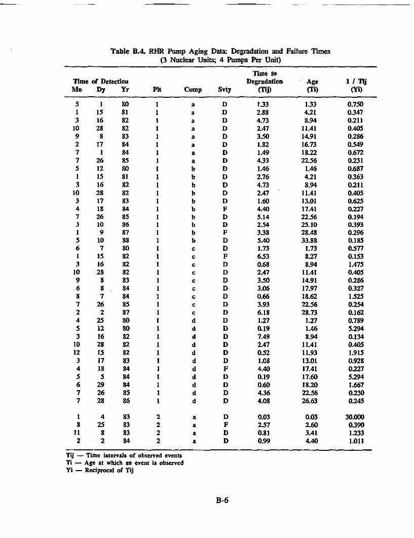
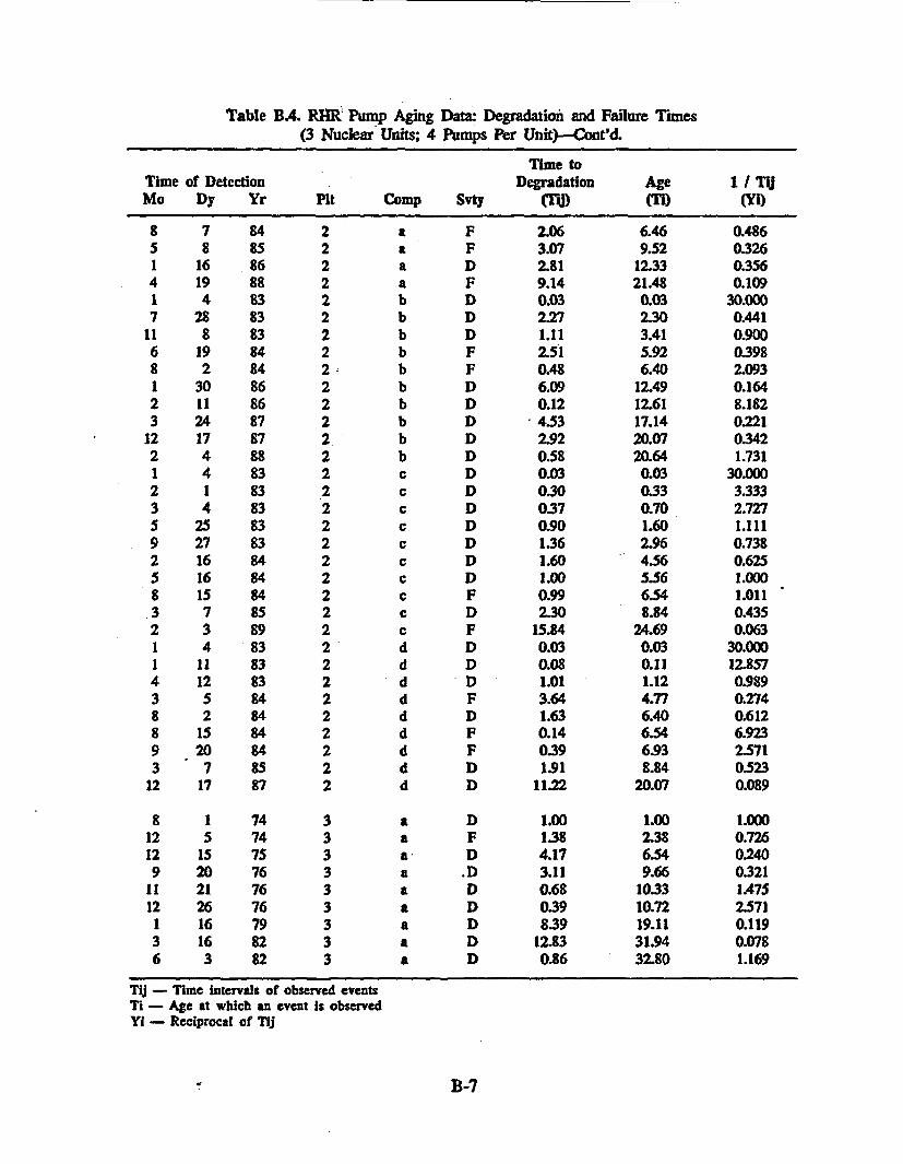
The process of data collection provides specific degradation and failure times of severalsimilar components (Appendix B). Focusing on the RHR pumps, data are obtained for agroup of components from different plants. In this case, the data covered three differentBWR units, each having four RHR pumps. The age of the plants differed, and the data didnot cover the entire life of the component in all cases.

Individually, the data for each of the pumps were insufficient to determine theparameters (degradation rate and aging failure rate). Accordingly, we studied a componenttype (the RHR pump) using data from the group of components (in this case, 12 RHRpumps). Statistical tests were conducted to justify the use of data across components andacross plants.

For SW pumps, data from seven BWR units out of twelve units were used in theanalysis. Based on the statistical tests, the SW pump aging data in the remaining five unitswere not compatible with the data from the seven units used in the analysis. Each of theseunits has three or more SW pumps, thus providing a data base from about forty three pumps.

19

Similar to the analysis approach in RHR pumps, statistical tests were conducted to justify theuse of data across components and across plants.

Statistical tests for use of data across components and across plants

The statistical tests were conducted with the following objectives:

1. to demonstrate that times between degradations (or between failures) across com-ponents within a plant are identically distributed, i.e., the components belong to thesame population for analysis of degradation and failure rate characteristics, and

2. to demonstrate that components across the plants belong to the same population.

The tests were conducted separately for degradation and failure data. Mann-Whitney U-tests and Kruskal-Wallis (K-U) tests were used, details of which are presented in AppendixC. The results showed that components could be grouped together: for the RHR pumps, thestatistical tests justified using data from twelve pumps across three different power plants. Inthe case of SW pumps, the test results justified use of data across seven units out of twelveunits.

Data were combined in two ways. In Method 1, the data on time to degradation or timeto failure were combined from different RHR pumps, i.e., separate data from each com-ponent were used to develop the data base. In Method 2, data from different componentswere "pooled", i.e., degradation and failure times obtained from each component wereplotted on a single time-line to obtain new degradation and failure times for the analysis. Inour terminology, we describe Method 1 as "data combining" and Method 2 is called "datapooling".

Trend testing and identification of age-groups with degradation and failure time

The data obtained by either of the methods ("data combining" or "data pooling") weretested for time-trends before developing age-related degradation and failure rates.

Statistical tests were used to define component age groups showing similar agingbehavior. We observed that early life showed a decreasing trend, and later life showed eitherincreasing or constant trends with time. Using regression analysis, data from age-groupswere appropriately partitioned that showed statistically significant time trends for developingaging rates.

5.2 Aging Effect on Degradation

The analysis of degradation data for the RHR pumps and SW pumps was conductedwith the following objectives:

1. identification of age-groups where statistically significant time trends exist, and

2. determination of the time-trends, and degradation rates, using regression analysis.

The details of the statistical analyses are presented in Appendices C and D. Here, we discussthe results and the characteristics of degradation rate.

20

Figure 3 shows the degradation rate and the logarithm of the rate that characterized theRHR pumps over ten years (presented as 40 quarters). On the vertical axis, ln4 of 2,presented on the right side, implies XD equal to 7.39, presented on the left side. Thedegradation times were obtained from plant-specific data bases of twelve RHR pumps, fourfrom each of three units (Appendix B). Statistical tests (in Appendix C) showed that thedegradation behavior across these components are similar, and accordingly, a genericdegradation characteristic was studied. Data combining and data pooling were studied: bothshowed similar results. The results obtained by data combining are discussed.

The following observations can be made from the age-dependent degradation rate forthe RHR pumps:

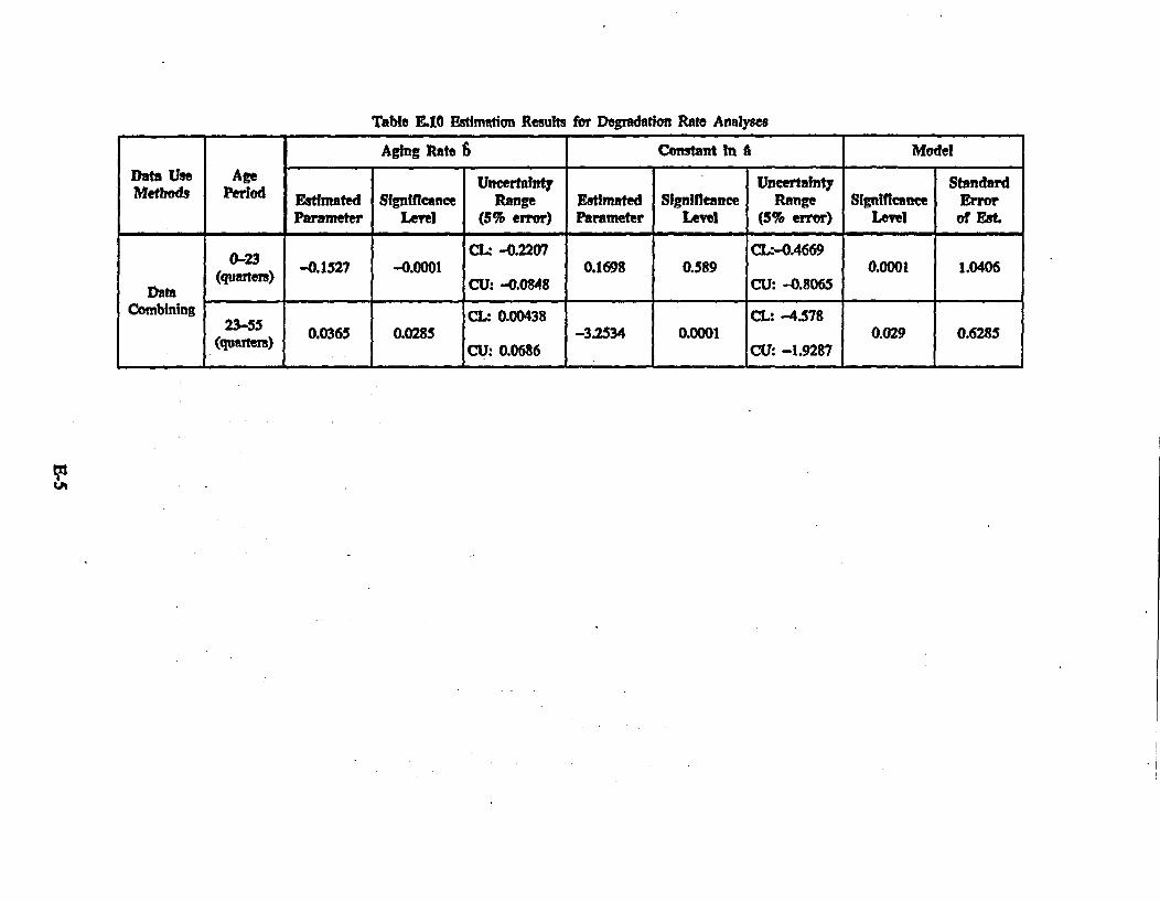
1. The degradation rate shows significant age-dependence; the early life of the com-ponent (i.e., first five years) shows a decreasing trend (significance level: 0.001),and the later five years show an increasing trend (significance level: 0.05), with theage of the component.

2. The increase in degradation rate, which is of interest in aging studies, is significant:the degradation rate increased by almost an order of magnitude at the end of tenyears.

3. The 95% confidence bounds for the degradation rate show that the uncertainty in theestimation is not large. The increased number of degradations observed in acomponent (compared to failure data) and the statistical approach taken for usingdata across similar components exhibiting similar degradation behavior contribute tolower range of uncertainty. This signifies that statistical methods can be used. toestimate degradation rates.

Figure 4 shows the logarithm of the degradation rate that characterized the SW pumpsover twelve years (presented as 50 quarters). The method of data combining was studied forSW pumps. The generic degradation characteristic was obtained by combining data acrossseven units consisting of forty-three pumps. Appendix E presents detailed results.

The observations on the age-dependent degradation rate for the SW pumps are asfollows:

1. The degradation rate shows age-dependence: the early life of the component (i.e.,first five years) shows a decreasing trend and the remaining seven years show anincreasing trend with the age of the component.

2. The increase in the degradation rate as the component ages is not as significant as inthe case of RHR pumps; nevertheless, the degradation rate is showing aging effecton the component During the later seven year period the rate increased by about afactor of 3.

5.3 Aging Effect on Failures

The aging-failure data for the RHR pumps and SW pumps were also analyzed with thefollowing objectives:

21

Degradation Rate 'AD( # per quarter)54.2

33.12 -20.09 -_ --__ _ _ _ _12.18 -7.39 - ____ __ ___

4.482.72 __ ____

1.65I fn _

In) ,

4

3- Estimated Eleg.Rate----

95% confidence bounds

Data Method 1 - Combining

-- Ouasl Cubic spline- fit -

2

0.81

0.370.220.14

0.080.050.030.02

1

I -2

-3

_-4400 10 20 30

Age in Quarters (3 month periods)

Figure 3. Age dependent degradation rate for RHR pumps(3 plant data)

FI IL L . . _ _-_ --. -40 10 20 30 40 50 60


Figure 4. Age dependent degradation rate for SW pumps(7 plant data)

22

1. identification of age-groups where statistically significant time trends exist, and

2. determination of aging-failure rates where time trends exist, and estimation of time-independent failure rate where time-trends cannot be established.

Again we discuss the results and the characteristics observed in the aging failure rateand give details of the analysis in the appendices. Appendices C and D present the detailedresults for the RHR pumps and Appendix E describes SW pump study. Figure 5 gives thelogarithm of the age-dependent failure for RHR pumps. The data base used covered the samecomponents as for the degradation rate. The statistical tests justifying the use of data acrosstwelve RHR pumps were the same, but the sparsity of data on aging failure required aslightly different analysis.

The aging-failure data for the RHR pumps show only a few failures during the later fiveyears of the components (age 5-10 years) and, in general, the number of failures was small.The statistical trend testing, based on both data combining and pooling, showed a decreasingtrend in the early life, but no trend in aging-failure could be established in the later fiveyears. Because of the sparsity of the data, isotonic regression analysis was used to estimatefailure rate for the first five years of RHR pumps where decreasing trend was observed. Forthe later five years, due to a lack of any trends, a constant, time-independent, failure rate wasestimated.

The following observations can be made from the aging-failure rate obtained for theRflR pumps:

1. The aging-failure rate shows decreasing trend in the first five years, but a constantfailure rate can only be estimated for later five years of the overall ten years. In otherwords, there was no trend of increasing failure with age for the ten-year operatingperiod of the RHR pumps.

2. The aging failure rate shows a behavior similar to the degradation rate in the earlyfive years, but differs after that. The aging-failure rate was significantly lower thanthe degradation rate and the difference increased with increasing age. The degrada-tion rate was about a factor of 30 higher than the aging failure rate at the end of 10years.

3. The 95% confidence bounds associated with aging-failure rate show higher uncer-tainty compared to the degradation rate, due to the few observations of failures.

Figure 6 gives the logarithm of the failure rate for SW pumps. For the SW pumps, onlya few failure data points were available for analysis. The sparsity of this data base is partlyattributable to the data source which is considered incomplete for the early life of thecomponents. Appendix B discusses the SW pump data evaluation and the associatedlimitations.

The available SW pump data were not adequate to detect any statistical trend withconfidence. Accordingly, no aging effect of the SW pump failures is established: a constantfailure for the study period (approximately 12 yrs.) is estimated.

23

1n4

3

2

1

0-1

-2

-3

-'-4400 10 20 30


Figure 5. Age dependent failure rate for RHR pumps(3 plant data)

InAlf

Failure Rate l A,. per quarter)54.6.4

20.0 -Estimated Failure Rate. In A,395% confidence bounds

7.39 2Data Method 1 - Combining

2.72 1

L O O 0

0.37 i

0.4

0.05ii fl .|'

I

2

3

4

0 10 20 30 40 50


Figure 6. Age dependent failure rate for SW pmps(7 plant data)

60

24

5A Aging Evaluation Using Degradation and Aging-Failure Rate

The analysis of the degradation rate and the aging-failure rate provides a comprehensivepicture of the aging process in the components studied (RHR and SW pumps) and providesinteresting insights on component aging.

1. The use of information on degradation and failure not only increases significantlythe information base for adequate analysis, but provides interpretations of the agingprocess that cannot be obtained by analyses of failure data alone. For both of thesepumps, degradation data indicate aging whereas failure data are yet to indicate agingtrends.

2. The aging trend in the degradation during the later 5 to 10 year period shows asignificant effect on component degradation as the RHR pump ages, but a simul-taneous lack of aging trend in the failure rate signifies that degradation has not beenmanifested in an increasing failure rate. Similarly, for the SW pumps, there is noaging effect on failures corresponding to the aging effect on degradations observedduring the later seven years of operation. In the degradation modeling approach thisfinding signifies that maintenance is effective in preventing age-related failures, andthat aging is represented through an increase in the degradation rate.

3. The relation between degradation and aging-failure rate in the first five years of theRHR pumps remained the same, i.e., both curves were similar and the degradationrate was steadily and consistently higher than the aging-failure rate. In the case ofSW pumps, the degradation rate was consistently higher than the failure rate, butthese rates show different behavior. However, failure data in the early life of SWpumps are considered incomplete.

4. The decreasing trend in the degradation rate for both pumps ends after the first fiveyears, and the rates show differences with the corresponding failure rates, starting atthis point.

5. Because there is more information on degradations, degradation rates are probablybetter indicators of aging than failure rates. Also, uncertainties in estimates ofdegradation rates are lower than those for aging-failure rates. Therefore, degradationrates can be effectively used to understand aging effects.

6. The relation between degradations and failures needs to be investigated further. Theincrease in degradation rate may be followed, after a time-lag, by an increasedfailure rate. The degradation rate, once it reaches a threshold value, may relate tofailure. Investigation of these aspects through degradation modeling may suggestwhen maintenances or overhauls of components should be performed to prevent age-related increase in failure rates.

5.5 Evaluation of Maintenance Effectiveness

As discussed in Chapter 3, the degradation modeling approach provides an estimate ofthe effectiveness of maintenance in preventing age-related failures. The transitionprobability from a maintenance state to failure state signifies the ineffectiveness of main-tenance in the simplified model studied. The complement of maintenance ineffectiveness ismaintenance effectiveness.

25

For the RHR pumps, the maintenance effectiveness is obtained (Figure 7) for each 10quarters of age. Effectiveness varies between 0.6 to 0.7 for the first 30 quarters, butsignificantly increases in the last 10 quarters. It is possible that effect of degradation onfailures is delayed and data beyond 40 quarters might provide better estimates of main-tenance effectiveness in the last ten quarters. The maintenance effectiveness for the SWpump (Figure 8) shows slightly different behavior. It declines in the early life and thenshows increase in the later life. As discussed, the relationship among degradations, failures,and maintenances is complex but extremely useful for studying aging in repairable com-ponents. A better understanding of this parameter will allow estimation of aging-failure ratebased on degradation rate estimates.

Maint. Effectiveness

I Estimated Maint. Effectiveness

0 10 20 30


40

Figure 7. Maintenance effectiveness(Component: RHR pumps; 3' plant data)

0 10 20 30 40 50


so

Figure 8. Maintenance effectiveness(Component: SW pumps; 7 plant data)

26

6. SUMMARY AND INSIGHTS OF DEGRADATION MODELING ANALYSIS

The report presents the concept of the degradation modeling approach in an agingevaluation of the safety system components of nuclear power plants. The use of degradationmodeling using information on component degradation was studied, along with the statisticalapproach to data analyses needed in such modeling. Applications to RHR pumps acrossthree nuclear units and SW pumps across seven nuclear units were'carried out to demon-strate the approach and the use of the modeling concept. In summary, we addressed thefollowing aspects to derive insights on the component aging process:

1. use of degradation information to develop a degradation modeling approach for usein aging studies,

2. statistical approach to the analysis of information on degradation failure, and

3. aging and maintenance effectiveness evaluation using degradation information.

As discussed in the report, the degradation modeling approach can have broader applicationsin aging reliability studies. The simple models presented provide interesting insights that aresummarized below, further developments and evaluations are necessary to develop this toolfor understanding and modeling component aging.

1. Benefit of using degradation information and degradation modeling

Aging is manifested through degradation of components. As presented in this report,analysis of degradations provides an understanding of aging that cannot be obtained bystudying 'age-related failures only. The other important aspect is that significantly moreinformation is available on degradations compared to failures, that is, how current practicesat plants are exhibited on component reliability and component reliability data bases.Degradation data enhance the data base for aging reliability and thus, the lack of dataproblem is reduced in this modeling approach.

2. Statistical approach to analysis of aging data

This report presents a statistical approach to analyzing aging data (degradation andfailure data). Statistical tests are presented to demonstrate the similarity of componentbehavior so that data can be taken from a group of components. Statistical trend tests arepresented to demonstrate the existence or lack of aging trends in the data before developingage-related rates using regression analyses. Using information on degradation and failurefrom twelve RHR pumps across three units, we demonstrated the statistical approach. Asimilar analysis is also presented for SW pumps. The uncertainty in the analysis also iscontrolled by using the statistical approach.

3. Aging evaluation using degradation modeling approach

In this report, RHR pump degradation and failure data were studied to understand theaging effect on the component. The result showed an aging effect on the rate of componentdegradation even though no aging effect on the aging failure rate could be established.

27

Similar results are also obtained for the SW pumps. The increase in the degradation rate maybe indicative of future increases in the aging failure rate. We showed that component agingcan be explained and demonstrated in a relatively short time studying degradations, whereasa much longer time is needed to demonstrate the aging effect through study of failure data.

4. Relations between degradations and failures

In degradation modeling, components are assumed to degrade in their path to age-related failures. This assumption is justified based on understanding of aging, but relationsbetween degradations and failures are not yet known. Plant maintenances and operatingpractices clearly play a role. A large number of possibilities that define the relationshipbetween degradations and failures exist, and deriving such relations will help define therequired maintenance practices and help develop component reliability models for agingstudies.

5. Evaluation of Maintenance Effectiveness

An important aspect of evaluating the aging process is to understand and characterizethe role of maintenance performed on the component. A simple model was studied, based ondegradation modeling approach, to obtain a parameter for maintenance effectiveness usingage-dependent degradation and failure rates.

This parameter can define why component aging failure rates are being controlled. Itcan also define when maintenance is ineffective to control component aging. The relation-ship among degradations, failures, and maintenance effectiveness are thus elemental inexplaining and modeling component aging reliability. The degradation modeling can furtherbe developed to better model the role of maintenance in component aging.

6. Model for component aging reliability

The analysis presented demonstrates that information on component degradation can beused to express aging effects on components, and that statistical approaches can properlyinterpret this data. A component aging reliability model should be developed that incor-porates this information and can take into account the effectiveness of maintenance inmitigating aging.

28

REFERENCES

1. D.R. Cox, Renewal Theory, Chapman and Hall, 1962.

2. D.R. Cox, Regression Models and Life Tables, J.R. Stat. Soc., B, 34, pg. 187-220.

3. W.E. Vesely and A. Azarm, System Unavailability Indicators, BNL Technical Report, A-3295-9-30-87, Sept. 1987.

4. STATGRAPHICS, Statistical Graphic System by Statistical Graphics Corporation, STSC,Inc., 1988.

5. NPRDS Program Description, Institute of Nuclear Power Operations, INPO-86-010,Atlanta, GA, 1986.

29

APPENDIX A. MATHEMATICAL DEVELOPMENT OF DEGRADATIONMODELING APPROACHES

A.1 Specific Degradation Models

Assume a component is being repaired and maintained. Assume, furthermore, that thecomponent experiences both degradations and failures. We wish to derive relationshipsbetween the rate of degradation and the rate of failure for the component in a givenenvironment and under a given test and maintenance program.

Degradation-Precedes-Failure Model

For one of the simplest models, we make the following assumptions:

1. Degradation always precedes failure'.

2. After a failure, a component is repaired to an operational state which reflects morerestoration than when on-line maintenance is performed.

3. When on-line maintenance is performed, the component is restored to a maintainedstate which reflects less restoration than when repair is performed after a failure.

We will call the state after a repair of a failure the "0-state." We will call the state aftermaintenance is performed the "m-state."

Equations for the Degradation and Failure Rates

Let

WD(t) = the degradation frequency at t (A-1)

WF(t) = the failure frequency at t (A-2)

*Then under the above assumptions and assuming the component was operational att = 0 we have the following balance equations for WD(t) and WF(t):

t r

WD(t) = fodt- 0) + Wf F()foD(te t) dt + f WD(t)fd(t, t) dt (A-3)0 0

and,

K

WF(t) = J WD(t)f,(te, t) dt (A-4)

where

A-1

foD(t, 0) = probability density for a first degradation occurring at t given the com-

ponent was restored to an operational state at t = 0

foD(t', t) = probability density that a first degradation occurs at t given the component

was restored to an operational state at t'

fmD(t', t) = probability density that a recurring degradation occurs at t with no inter-

mediate failure given the component was maintained at t'

fDF(t', t) = probability density that a failure occurs at t with no intermediate observed

degradation given the component was degraded and maintained at t'

We will call fOD(t', t), fMD(t', t), fDI(t', t) transition probability densities.

Function Forms for the Transition Probabilities

For general time-dependent and age-dependent modeling the transition probabilitydensities are functions of both t' and t, or equivalently, are functions of t' and t - t'. Forage-dependent evaluations, for example, t' is the age of the component and t - t is theinterval involved. For steady state modeling which we first address, the transition probabilitydensities are functions only of the interval t - t'. We distinguish these cases below.

General Time Dependent and Age Dependent Functional Forms

foD(t', t) = foD(t", t -t) (A-9)

fMD(t', t) = fMD(t', t - t') (A-10)

fDF(t, t) = fDF(t, t - t) (A-Il)

Steady State Functional Forms

foD(t, t) = foD(t - tO) (A-12)

fMD(t, t) = fMD(t - t) (A-13)

fDF(Q t) = fDF(t - t) (A-14)

Steady State Failure and Degradation Equations

WD(t) = foD(t) + f WF(x)foD(t - x) dx + WD(x)fDF(t - x) dx (A-15)

A-2

K

WFt) f WD(X)fDF(t x) dx (A-16)

Asymptotic Solutions

As t -+ oo the asymptotic, steady state solutions for WD(t) and WF(t) are:

WD = WFPOD + WDPMD (A-17)

WF = WDPD (A-18)

where,

POD = limit L fOD(t -X) dx fOD(X) dx(A-19)

PUD = limit f1 D(t -x) dx=| fu1 (x) dx (A-20)

DF = limit _ fF(t x) dx= fDf(x) dx (A-21)

The terms POD PmD , PDF are corresponding transition probabilities:

POD = probability that a degradation occurs after the component is restored (A-22)

with no failure before a degradation

= I under our assumption (A-23)

PmD = probability that a degradation occurs after a maintenance before a (A-24)

failure occurs

PDF = probability that a failure occurs after a degradation and maintenance (A-25)

with no intermediate degradation

Solving the Steady State Solutions

The steady state balance equations are again

WD = WFPOD + WDPMD (A-26)

WF = WDPDF (A-27)

A-3

Under our model POD = 1 as indicated and hence,

WD = WF + WDPMD (A-28)

WF = WDPDF (A-29)

From the above two equations we have,

W =I + W PMD (A-30)

WD I PPMD _PDF + PMD 1(A-31)

WF PDF PDF PDF

PMD -WD (A-32)PDF WF

PMD -W - WF (A-33)PDF WD

Interpreting the Steady State Relation

The steady state solution is again:

WD = ' (A-34)WF PDF

or

PDF = W (A-35)WD

Interpretations:

1. The larger the ratio WF / WD , the larger is the probability that a failure will occurafter degradation PDF-

2. For a given degradation frequency WD, the larger the probability PDF' the larger isthe failure frequency WF.

3. The ratio WF / WD is a measure of maintenance ineffectiveness in that it is equal toPDF. However, smaller values of PDF can result in larger values of WE if WD islarger.

A-4

4. Another measure of maintenance effectiveness is the failure frequency WF itselfwhich is equal to WDPDF.

5. The ratios WF / WD can be calculated for various components and failure modes.Statistical relationships involving WF / WD, component types, failure modes, andfailure causes can be investigated.

6. The ratios WF I WD, or equivalently PDF, can be used to predict WF from knowledgeof WD under different scenarios, e.g. under aging scenarios.

Incorporation of Aging Effects

Assume aging occurs. At some threshold time (age to), the failure frequency WF anddegradation frequency begin to increase with age. Under what constraints will the sameprobabilities PDF and PmD which applied to the steady-state case also apply to the agingcase? To answer this question consider again the general time dependent balance equations:

t o

WD(t) = fOD( 0. t) + [ WF(x)fOD(x, t - x) dx + | WD(x)fm(x, t - x) dx' (A-36)

WF(t) = WD(x)fDr(x, t - x) dx (A-37)

Translating the origin to to gives:

t

WD(t) = foD(to t - to) + | WF(x)f6(x, t - x) dx + W1D(x)fmD(x, t - x) dxto t (A-38)

WF(t) = f WD(X)fDF(X, t - X) dx (A-39)to

Assume again the transition probabilities are only dependent upon the interval t - x, i.e.,

foD(to, t - to) = fOD(t - to) (A-40)

fMD(x, t - x) = fMD(t - x) (A41)

foD(X, t - x) foD(t - x) (A42)

Then PDF and PD will be the same as for the steady state case and the relations for WF(t)and WD(t) in the aging case are given by:

t

WD(t) - foD(t to) + f WF(x)foD(t - x) dx + | WD(X)fdt - x) dx (A-43)Jto to

A-S

toWA~) =f WD(x)fDr.(t - x) dx (A-44)

The last equation for WF(t) is the particularly relevant equation for predicting the failurefrequency from the observed degradation frequency. If WD(x) was observed and fDF(t - x)were known, then WF(t) could be predicted from the above equation. Assuming the samefDF(t - x) as in steady-state behavior allows fDF(t - x) to be estimated from steady statedata to apply to aging monitoring and prediction, we study models for the transitionprobability distributions.

Models for the Transition Probability Distributions

The simplest models for fmD(x), fF(x), and foD(x) involve assuming a constant rate oftransferring from one state to another. Let:

XMD = the rate of a degradation occurring after a maintenance when (given) (A-45)

no previous degradation has occurred

XDP = the rate of a failure occurring after a degradation when (given) no (A-46)

previous failure has occurred

XOD = the rate of a degradation occurring after an operational restoration (A-47)

when (given) no previous degradation has occurred.

Assume that XMID, XDF, and XOD are constant. Then fmD(x), fmpx), and fOD(x) are given by:

AMDfmDjx) = ).D exp(-),mx) = T- IM exp(-X1Mx) (A-48)

)LDFfDF(X) = 4pF exp(-4Lx) = M exp(-)iMX) (A-49)

and

fOD(x) = OD eXP(-XD4 X) (A-50)

where

XM = XDF + LMD (A-51)

Estimation of the Transition Rates

The probability PDF is given by:

A-6

PDF = | F exp(-)jmx) dx = - |;A. epX ) Adx (A-52)

or,

A'DF (A-53)

Therefore, the ratio XDF / XM can be estimated from the ratio WF I WD since WF =WDPDF.

The degradation rate Am also needs to be estimated. In general, ;m is age dependenteven if we assume the ratio I., / m is constant. One scenario under which the ratio is thesame but the transition rates can be age dependent is where the transition rates have the sametime dependence:

=DF kDFg(t) (A-54)

)DM= kMDg(t) (A-55)

where g(t) is a general time dependent or age-dependent function with possibly a thresholdtime to, i.e.

g(t) = 1 t < to

= h(t) t > to

In the above case the ratio of XDF / X will not be time dependent or age dependent:

)DF kDF (A-56)

AM kDF + kMD

To estimate 'D in the age-dependent scenario, assume we observe times of degrada-tions when the component is aging:

Times of degradations: t1, t2,...t. (A-57)

Also, we may observe times of failures when the component is aging.

Times of failures: ul,...,um (A-58)

We will not use the times of failure to estimate the transition rates since we may nothave times of failures. When we have them, we can use them to check and refine the model.

A-7

Likelihood Estimation

Assume the times of degradation are measured with regard to the threshold time. Thenthe likelihood L for the times of degradation is:

L = XMD(tI)XMD(t2) ... MD(tQ) exp XM(x) dxj (A-59)

where,

XMW = XMV(x) + XDF(X) (A-60)

and,

t,, = to, Time of last degrdation only measured. (A-61)

tmnax = tend, An observation time from t. to ta, is also recorded (A-62)where there are no further degradations.

The above likelihood thus is a standard function which can be used to estimate parametricforms (e.g., Weibull or exponential) for XmD(s) [and XDF(s) using the determined ratioestimate kMF / (kMF + k1mo9. Thus we can predict the aging failure frequency using thebalance equation for WF(t) and the steady state ratio kD0 / (kDF + kmD).

A-8

APPENDEX B. DATA BASE FOR AGING DEGRADATION AND FAILURE

B.1 Data Analysis

Data on degradation and aging failure were obtained for the analysis from themaintenance history of the components. The maintenance history includes activities (such aspreventive and corrective maintenances, and testing) performed on the components from theday of its installation. Two sources of data were solicited: plant specific maintenance recordsand component reliability data base in Nuclear Plant Reliability Data System (NPRDS).

Data were collected for specific types of components where the maintenance history foreach component was studied. We developed degradation and failure data bases for two typesof components (residual heat removal (RHR) pumps, and service water (SW) pumpssupplying cooling water to the RHR system). RHR pump data were obtained from plantmaintenance records, whereas NPRDS (Ref. 5) was used for SW pump data. Both of thesesources have individual component identification that is essential for obtaining the type ofdata desired for degradation modeling. The RHR pump data were taken from three BWRunits, each consisting of four identical pumps. The SW pump data covered thirty-three BWRunits in the NPRDS database, from twelve units experiencing 10 or more failures in each ofsix or more SW pumps.

B.2 Data Classification

Each record of maintenance or reported failure was classified into three categories, asdefined in Table B.1. Plant-specific data, taken from the maintenance log, contain all threekinds of data, whereas the NPRDS covered mostly D and F type information. For this study,the N type of information is not used in the model, and hence, were not collected in this dataanalysis. However, this information will be useful later in judging the current preventivemaintenance practices which can improve the maintenance effectiveness in a component.

Although these categories are not directly correlated with the severity levels (incipient,degraded, catastrophic) defined in NPRDS, comparing with NPRDS categorization it can be

Table BA. Categorization of Component Failure or Maintenance Data

Category Description

N Activities such as routine checks, inspections and testing that indicated nosign of degradation in the component. No particular maintenance wasperformed.

D Activities indicating definite degradation in the component subassemblies.Maintenance was performed to ameliorate the degraded condition of thecomponents.

F Activities indicating degradation in the component such that it requiredimmediate maintenance to be able to perform its design function.

B-l

noted that most incipient type failure data in NPRDS were categorized as type 'D' and somedegraded data were judged type 'F' for this analysis. All of the catastrophic data werejudged to be of 'F' category. Therefore, each record (identified in plant-specific maintenancehistory or NPRDS) was judged for relevance to age-related degradations and failures, andthen was placed into one of the three categories.

Table B.2 lists the maintenance records for one RHR pump taken from a plantmaintenance work request (MWR) or work authorization (WA) log list, and demonstratesthe categorization of each of the items according to the scheme defined in Table B.1. Thedescription of each of the records was used to classify the record in one of the threecategories, as shown in, the last column (N, D, or F). The data for the SW pumps were takenfrom the NPRDS and are shown in Table B.3. Again, the last column of this figure indicatesthe classification of each record. We note that this categorization is at variance with theseverity classification (catastrophic, degraded, and incipient) used in NPRDS. The reason isthat NPRDS is not directed at aging evaluations, whereas this data analysis focussed onidentifying age-related degradations and failures.

Table B± Maintenance Log for an RHR Pump at a BWR Unit

DESCRIPTION IDENT. FAILUREWA # EQUIP. I (ACTION TAKEN) DATE CLASS.

P21906 IP202B ANNL PM-RHR PMP MOTOR INSPECTION 12115132 NOIL SAMPLES TAKEN/NO LEAKS FOUND

S24999 IP202B INST VIB PICKUP MOUNT LOCATIONS FOR VIBRO PACK 7108102 NPICK UP ON RHR

CANCELLED-NO WOCRX WILL IE PERFORMED UNDERTHIS WA

U24318 IP202B REBUILD MECH SEAL THAT WAS REMOVED FROM PUMP 3/16182 DREBUILT SEAL, NEW -0w RINGS & SEAL FACESRETURNED TO STORES

P30491 IP202B ANNL PM-RHR PMP SEAL HT XR 3/17/83 DCLEANED, INSPECTED, REPLACED GASKETS, REASSEM-BLED, TORQUED TO 30 FrALBS. CLEANED AND IN-SPECTED HELIFLOW COOLET AS PER IOM 153.

P31444 IP202B EQ QL-RHR PUMP MOTORS 9/08/83 NREMOVED OIL SAMPLES FROM UPPER & LOWER BEAR-INGS. OK IS IN THE CHEM LAB. OIL LEVELS WERE ATTHE PROPER LEVEL SCREENS ON MOTOR WERE CLEAN.SPACE HEATERS OK.

P40859 1P202B ANNL PM-RHR PMP SEAL HT XR 4/1834 FA NEW SEAL WATER COOLER WAS INSTALLED UNDERWA #C44042 PMR 84-3014 DURING THE UNIT 1/UNIT 2 TIEIN OUTAGE. INSPECTION IS NOT NECESSARY AT THISTIMa

N - No Degradation/failure D - Degradation F - Failure

B-2

Table B3. NPRDS Reported Data on SW Pumps

FAILURE FAILURE UnLrTY IN-SERYSTART END UNIT COMPONENT DATE FAILUREDATE DATE ID ID FAILURE NARRATIVES (COMP) CLASS.

04112/32 05/30/2 GPCEMI P41-C0IA PLANT SERVICE WATER PUMP FAILED TO MEET REQUIRE- 12t31/75 FMENTS OF ASME SECTION II nWMOP0 THE CODE'S INTENT ISTO TRACK PUMP PERFORMANCE AND TO ASSURE THE PUMPPERFORMS PROPERLY. TE CAUSE OF THE FAILURE WAS DUETO NORMAL WEAR AND NATURAL END OF LIF THE PUMPWAS REBUILT AND SATISFACTORILY TESTED AND RETURNEDTO SERVICE.

04/O2/4 040/84 GPCEIHI P41-C0IA DURING PLANT OPERATION. OPERATIONS PERSONNEL DETER- 12/31/75 FMINED THAT THE PLANT SERVICE WATER PUMP'S SHAFTSEAL WAS LEArNo EXCSSVELY. REF MR 1-84-1335 FAIUEWAS CAUSED BY WEAR AND ABRASIVE WATER THE PUMP'SSHAFT SEAL WAS REPLACED WITH A NEW ONE. THE PUMPSEAL WAS 7THN SATISFACTORILY TESTED.

06/02/35 10)0/35 GPCEIHI P41-001A WHILE OPERATING AT RATED FOWE OPERATIONS PERSON- I2V3175 DNEL DETERMINED THAT PLANT SERVICE WATER PUMP "AWAS OPERATING AT A DECREASED FLOW AND PRESSURE.THERE WAS NO EFFECT ON THE PLANT. (REF MWO'S 18503078,A8564 18503227 AND DCR 84-59) THE CAUSE WAS AT-TRIBUTED TO EROSION OF THE PUMP INTMNALS (NORMALWEAR). CAUSING LEAKAGE PAST THE MLLER TO THM SUC-TION SIDE OF THE PUMP. THIS WAS A CARBON STEEL PUMP.THE INTERNALS, DISCHARGE CASE AND SUCTION BELL OFTHE PUMP WERE REPLACED WITH STAINLESS STEEL PARTSPER DESIGN CHANGE THE PUMP WAS OPERATIONALLYCHECKED AND PERFORMED AS EXPECTED.

05111/87 06/18/87 GPCEIHI P41-0I1A DURING A PLANT REFUELING OUTAGE. OPERATIONS PERSON. 12/31/75 DNEL LOCATED A SMALL LEAK ON THE A PLANT SERVICEWATER PUMP COUPLING. THIS DID NOT CAUSE ANY CHAN-GES IN PLANT PARAMETERS. REP: MWO 1-37-03880. THECAUSE OF THE LEAK WAS FOUND TO BE A HOLE IN THECOUPLING COOLING WATER LINl THIS WAS ATTRIBUTED TONORMAL/CYCLIC WEAR. THE COOLING COIL WAS REMOVEDAND REPAIRED. AFTER TESTING IT WAS REPLACED AND THEPUMP WAS RETURNED TO SERVICE.

D - Degmdation P - Failure

ww

For each component, a time-line plot was generated indicating the age of the componentand times of degradations and failures based on maintenance data for the life of thecomponent. Figure B.l shows an example of such a plot. The in-service date for thecomponent is considered the beginning of life for the component. Following replacement oroverhaul, components were treated as new, i.e., as if the component was at the beginning oflife.

The age of the component was calculated by the difference between the component in-service date (or overhaul date) and the problem identification date for maintenance. The agewas expressed in quarter years. All maintenance records (types N, D, and F) for eachcomponent were plotted in a time-line fashion to recognize any patterns in the records(Figure B.1).

Data for Statistical Analysis

Two types of data, time to degradation (TTD) and time to failure (TTM), weredeveloped for each component from the time-line plots. The 1TD was used to obtain thedegradation rate, while the TTF was used to obtain the failure rate of the component.

Both F- and D-type records were used to calculate ITD. In estimating the TTF, only F-type records were used. Both these parameters (TTD and TTF) are obtained as a function ofcomponent age from the maintenance records categorized as D or F. Continuity in themaintenance records was important to obtain this data.

Data Source Limitations

It was difficult to obtain complete maintenance records of aged components. Specifical-ly, recently built plants have computerized lists of their maintenance activities and, thus,provide all three record categories (i.e., N, D, and F types). But they cover only the earlyyears of a component's life. On the other hand, older plants did not have such a system at an

TIME TO TIME TODEGRADATION FAILURE

(TTD) (TTF)

01D N F D F

AGE IN QUARTERS

Figure B.1. Example of time-line of plot of degradation (D) and failure (F) times

By

early age, so that information relating to their early life was not readily available in a formneeded for this analysis. However, after the plant adopted a computerized system, the datawere as complete as the new plants.

The data obtained from NPRDS are not as complete as those obtained from plant-specific maintenance records. Since utilities are not required to report all maintenanceactivities to NRPDS, only some maintenance of the component are obtained. Furthermore,data over the entire operating life are not always available in the data base.

RHR Pump Aging Data

Aging data on RHR pumps are obtained by analyzing plant maintenance records forthree units. Since the units are of different age, data for RHR pumps in each covereddifferent periods: 34 quarters for Unit 1, 25 quarters for Unit 2, and 50 quarters for Unit 3(Table B.4). This table contains the observed dates both for degradations and failures. TableB.5 presents the failure data where only the observed failure times are recorded. As thesetables show, significantly larger information on component aging is obtained by focussingon degradation data.

SW Pump Aging Data

Aging data on SW pumps supplying water to the RHR system were obtained from theNPRDS data base. The data gathered from twelve plant units were tested statistically fortheir compatability. Only seven units are found to have compatible data, and accordinglydata from these plants were used in the analysis. Since each unit has three or more SWpumps, data from a total of forty three SW pumps form the data base for this evaluation.Table B.6 lists the pump data, except those relating to the pump seals.

A large number of data for the SW pump was related to degradation or failure of pumpseals. Since these pumps use cooling water from an external source (e.g., sea, river, orpond), seal degradation/failures are in many cases attributed to intrusion of sands, sea weeds,and other external materials. These seal failures are not attributable to normal aging of theseals and hence, were excluded from this study.

In many cases, the data on a SW pump covered a brief period of the componentoperating life. This sparse data for a pump can create difficulty in calculating the time todegradation (TD) and the time to failure (ITF). Since the available data period did notnecessarily cover the beginning of life of the component, the first failure/degradationoccurrence was used to obtain TlTD or TTF. Thus two data points are required to calculateone TTF data (see Figure B.1). This difficulty resulted in a small data set for SW pumpfailure analysis. Therefore, Table B.7 which lists the failure data contains only five datapoints while Table B.6 has identified a number of data points categorized as type 'F'.

Because of these difficulties, the NPRDS data source is found to be less usefulcompared to the maintenance records from a plant. Furthermore, the NPRDS data base for acomponent appears incomplete in comparison to plant maintenance records. In conductingdegradation modeling analysis, a complete data of all detected degradations and failures arerequired which necessitate use of plant data bases that contain information collected duringall test and maintenance of the component.

B-S

Table B.4. RHR Pump Aging Data: Degradation and Failure Times(3 Nuclear Units; 4 Pumps Per Unit)

lIme toTime of Detection Degradation - Age 1 1 7IjMo Dy Yr Pit Comp Svty (MDj) (TO) (Yi)

5 1 80 11 15 81 13 16 82 1

10 28 82 19 8 83 12 17 84 17 1 84 17 26 85 15 12 80 11 15 81 13 16 82 1

10 28 82 13 17 83 14 18 84 17 26 85 13 10 86 11 9 87 15 10 88 16 7 80 11 15 82 13 16 82 1

10 28 82 19 8 83 16 8 84 18 7 84 17 26 85 12 2 87 14 25 80 15 12 80 13 16 82 1

10 28 82 112 15 82 13 17 83 14 18 84 15 5 84 16 29 84 17 26 85 17 28 86 1

1 4 83 28 25 83 2

11 8 83 22 2 84 2

a Da Da Da Da Da Da Da Db Db Db Db Db Db Fb Db Db Fb Dc Dc Fc Dc Dc Dc Dc Dc Dc Dd Dd Dd Dd Dd Dd Dd Fd Dd Dd Dd D

a Da Fa Da D

1.332.884.732.473.501.821.494.331.462.764.732.471.604.405.142.543.385.401.736.530.682.473.503.060.663.936.181.270.197.492.470.521.084.400.190.604.364.08

0.032.570.810.99

1.334.218.94

11.4114.9116.7318.2222.56

1.464.218.94

11.4113.0117.4122.5625.1028.4833.88

1.738.278.94

11.4114.9117.9718.6222.5628.73

1.271.468.94

11.4111.9313.0117.4117.6018.2022.5626.63

0.032.603.414.40

0.7500.3470.2110.4050.2860.5490.6720.2310.6870.36302110.4050.6250.2270.1940.3930.2960.1850.5770.1531.4750.4050.2860.3271.5250.2540.1620.7895.2940.1340.4051.9150.9280.2275.2941.6670.2300.245

30.0000.3901.2331.011

Tij - Time intervals of observed eventsTi - Age at which an event is observedYi - Reciprocal of Tij

B-6

Table BA. RHR Pump Aging Data: Degradation and Failure Times(3 Nuclear Units; 4 Pumps Per Unit)-Cont'd.

1Tme toTime of Detection Degradation Age 1 / Ti,Mo Dy Yr Pit Comp Svty aTJ (TOi) (YT)

8 75 81 164 191 47 28

11 86 198 21 302 113 24

12 172 41 42 13 45 259 272 165 168 153 72 31 41 114 123 58 28 159 203 7

12 17

848586888383838484868687878883838383838484848589838383848484848587

222222222222222222222222222222222

aaaabbbbbbbbbb

ccccccccc

dddddtddd

FFDFDDDFFDDDDDDDDDDDDFDFDDDFDFFDD

2.063.072.819.140.032.271.112.510.486.090.12

.4.532.920.580.030.300.370.901.361.601.000.992.30

15.840.030.081.013.641.630.140.391.91

11.22

6.469.52

12.3321.480.032.303.415.926.40

12.4912.6117.1420.0720.640.030.330.701.602.964.565.566.548.84

24.690.030.111.124.776.406.546.938.84

20.07

0.4860.3260.3560.109

30.0000.4410.9000.3982.0930.1648.1820.2210.3421.731

30.0003.3332.7271.1110.7380.6251.0001.0110.4350.063

30.00012.8570.9890.2740.6126.9232.5710.5230.089

8 1 74 312 5 74 312 15 75 39 20 76 3

11 21 76 312 26 76 3

1 16 79 33 16 82 36 3 82 3

a Da Fa Da Da Da Da Da Da D

1.001.384.173.110.680.398.39

12.830.86

1.002.386.549.66

10.3310.7219.1131.9432.80

1.0000.7260.2400.3211.4752.5710.1190.0781.169

Tij - Time intervals of observed eventsTi - Age at which an event is observedYi - Reciprocal of Tij

1� B-7

Table B.4. RHR Pump Aging Data: Degradation and Failure Tumes(3 Nuclear Units; 4 Pumps Per Unit)-Cont'd.

Time toTime of Detection Degradation Age 1 / TijMo Dy Yr Pit Comp Svty CTij) (Ti) (Yi)

10 23 82 3 a D 1.56 34.36 0.6432 25 83 3 a D 1.41 35.77 0.7093 3 85 3 a D 8.20 43.97 0.1227 1 86 3 a D 5.37 49.33 0.1864 23 75 3 b F 3.97 3.97 0.252

12 18 78 3 b D 14.78 18.74 0.0683 10 82 3 b D 13.13 31.88 0.0764 4 82 3 b D 0.27 32.14 3.7505 1 82 3 b D 0.30 32.44 3.3336 8 82 3 b p. 0.41 32.86 2.4328 1 82 3 b D 0.59 33.44 1.698

10 23 82 3 b D 0.91 34.36 1.0982 9 83 3 b D 1.23 35.59 0.8113 1 85 3 b D 8.36 43.94 0.1204 23 82 3 c D 32.36 32.36 0.031

10 23 83 3 c D 6.06 38.41 0.1653 1 85 3 c D 5.53 43.94 0.1819 14 74 3 d F 1.48 1.48 0.6773 18 76 3 d D 6.16 7.63 0.162

11 4 76 3 d D 2.51 10.14 0.3985 1 82 3 d D 22.30 32.44 0.045

10 23 82 3 d D 1.91 34.36 0.52312 1 82 3 d D 0.42 34.78 2.368

I I 83 3 d D 0.39 35.17 2.571I 1 84 3 d D 4.06 39.22 0.2473 1 85 3 d D 4.72 43.94 0.212

Tij - Time intervals of observed eventsTi - Age at which an event is observedYi -. Reciprocal of Tij

B-8

Table B.S. RHR Pump Aging Failure Data (3 Nuclear Units; 4 Pumps Per Unit)

Pit Compt FI; PYi

1 2 17.41 17.41 0.0571 2 11.07 28.48 0.0901 3 8.27 8.27 0.1211 4 17A1 17.41 0.0572 1 2.6 2.6 0.3852 1 3.86 6.46 0.2592 1 3.07 9.52 0.3262 1 11.96 21.48 0.0842 2 5.92 5.92 0.1692 2 0.48 6.4 2.0832 3 6.54 6.54 0.1532 3 18.15 24.69 0.0552 4 4.77 4.77 0.2102 4 1.77 6.54 0.5652 4 0.39 6.93 2.5643 1 2.38 2.38 0.4203 2 3.97 3.97 0.2523 4 1.48 1.48 0.676

FT3 - Time intervals between observed failuresF - Age at which an event (failure) is observedFi - Reciprocal of FTU

B-9

Table B.6. SW Pump Aging Data: Degradation Times(7 Nuclear Units)

rime toTime of Detection Degradation Age 1 / TiJMo Dy Yr Pit Comp Svty Dscp MTD) (Ti (Yi)

3 73 78 141 127 107 107 10

12 43 83 157 175 15

11 225 11

10 226 142 25

12 133 35 155 233 148 85 123 3

10 286 34 177 24

12 186 118 6

10 165 316 22I 15 12

74 474 486 584 374 474 474 486 580 786 786 786 583 581 785 287 1176 485 386 386 386 382 786 282 785 586 285 586 578 486 587 585 780 486 786 787 787 7

d d pumpa f pumpg f drainc f pumpc d impela d impeld d impelg f gasketd d pumpb f impelb d pumpa d impelh d coolera f pumpb f suppi d brgsg f brgsc d flangec d brgsd f brgse d lubec d pumpd d sepd d pumpc d pumpc d motord f valveb f brgsh f brgsb d pipec d pumpd d brgsc f pumpa f pumpc f diffug d brgsc f pump

0.180.180.370.511.541.371.371.222.092.421.360.805.796.847.687.828.161.080.949.99

10.0810.2710.91

8.8211.022.170.41

15.5717.922.688.30

13.1012.804.18

17.315.563.61

0.180.180.370.511.541541.541.592.092.423.784.015.796.847.687.828.168.249.199.99

10.0810.2710.9110.9111.0211.8012.0215.5717.9218.2420.2224.0126.9427.3427.5829.7331.19

5.6255.6252.7271.9570.6470.7320.7320.8180.4790.4130.7381.2500.1730.1460.1300.1280.1230.9281.0590.1000.0990.0970.0920.1130.0910.4622.4320.0640.0560.3730.1200.0760.0780.2390.0580.1800.277

Tij -Time intervals of observed eventsTi -Age at which an event is observedYi- Reciprocal of Tijimpel - impellerbrgs - bearingssupp - support (hangers, snubbers)sep - separatordiff -diffuser

lube - lube oilp-Dl - pump-motor

B-10

Table B.6. SW Pump Aging Data: Degradation Times(7 Nuclear Units)-Cont'd.

Time toTime of Detection Degradation Age I/ rTiMo Dy Yr Pit Comp Svty Dscp (Ti) (Ti) (YI)

3 25 886 2 856 25 824 4 885 11 878 27 858 28 87

11 14 857 30 867 1 881 18 876 10 876 17 85

10 5 85

76

11264644b441111

d d brgsa f pumph d p-ma d pumpa d coolere d drain° f brgsb d pumpb d pumpc d pipeb d pumpb d draind d ventf d puMP

10.714.720.04

10.177.88

11.9910.664.662.903.421.921.58

12.6914.06

34.7238.2343.4844.7946.1146.647.3047.5350.4350.7252.3653.9355.5656.76

0.0930.212

22.5000.0980.1270.0830.0940.2150.3450.29205200.6340.0790.071

Tij- Time intervals of observed eventsTi -Age at which an event is observedYi- Reciprocal of Tijimpel - impellerbrgs - bearingssupp - support (hangers, snubbers)sep - separatordiff - diffuserlube - lube oilp-m - pump-motor

Table B.7. SW Pump Aging Failure(7 Plants)

Data Trnes

row Mo Dy Yr Pit Comp Svty Dscp FT'U F1M FYi

1 12 4 86 5 g f gasket I222 1.59 0.8192 6 3 85 5 d f valve 12.020 12.02 0.0833 5 31 86 7 a f puMp 20.500 27.34 0.0484 5 12 87 7 c f puMp 20.920 31.19 0.0475 6 2 85 6 a f pump 38.230 38.23 0.026

FTij - Time intervals between observed failuresFTi - Age at which an event (failure) is observedFYi - Reciprocal of FTij

B-11

APPENDIX C. STATISTICAL TESTS ANALYSES FOR DATA FROMDIFFERENT RHR PUMPS IN DEGRADATION AND FAILURE RATE

This appendix summarizes the statistical tests performed on degradation and failure dataof the RHR pumps. The specific statistical tests and their purposes are as follows:

1. Tests to identify the similarity of degradation and failure of RHR pumps within anuclear unit

a. Mann-Whitney (M-W) U Test

b. Kruskal-Wallis (K-W) Signed Rank Test

2. Test to identify the similarity of degradation and failure behavior across nuclearunits

a. Mann-Whitney (M-W) U Test

b. Kruskal-Wallis (K-W) Signed Rank Test

3. Test to identify periods where there are significant time trends in degradations andfailures

a. Mann's Rank Test.

In the following, we briefly explain the tests performed and the results obtained. Onlyrepresentative results are presented; similar results are obtained in other cases as indicated inthe text.

C.1 Mann-Whitney U Tests for RHR Pumps Within Each Nuclear Unit

The Mann-Whitney U Test is conducted, based on the degradation data set, to see if thetimes between degradation TU, (or equivalently 1 I TV) in each of the 4 pumps are identicallydistributed withini each of the 3 plants. The Mann-Whitney procedure is designed for tests oftwo independent samples; it is a variation of the Wilcox rank-sum procedure, and thecomputational form of its statistic U uses the rank sum. The test combines and ranks the datafrom two samples; these ranks are then summed over all observations in each sample and thestatistic U1 is calculated as follows to compare the average ranks:

+ 1)-U1 = nn 2 + 2 ) 1

(2

ws ornks a T

where T, = sum of ranks associated with Xi values (i _1, 2), and

C-1

n, = sample size of Xi .

In our degradation data sets most samples have more than 10 observations, therefore, a.iormal approximation of test statistic Z is used in the test.

U - Ru

where,

Inii

R.= 2 and = 12 fI12 1I ni

The main assumptions of the Mann-Whitney Test are satisfied in our data, that is:

a. the samples are independent, and

b. the populations are identical except for possible differences in location.

However, in reality the Mann-Whitney Test enables us to identify any differences in theunderlying distributions although it is particularly sensitive to differences in location (interms of medians or means). Therefore, it is a strong statistical test to identify whethercomponents belong to the same population.

The Mann-Whitney Test for each pair in each of the three plants did not reject the nullhypothesis of identical samples (based on comparison of average ranks and significancelevel of 0.05). Table C.1 presents the results for the pumps in one of the plants; similarresults are obtained for all three plants. Null hypothesis of identical samples was not rejectedin any of the cases. Accordingly, the degradation behavior of the four RHR pumps belongedto the same population in each of the plants.

Table C.L M-W Test Results for RHR Pumps in Plant 1

Average # of Values Average # of Values TestComparison of Rank of of 1st Sam- Rank of of 2nd Total Statistic P

Samples Ist Sample ple 2nd Sample Sample Observ. Z Value

Compt 1-Compt 2 10.75 8 8.5 10 18 -0.845 0.398

Compt 1-Compt 3 9.25 8 8.77 9 17 -0.145 0.885

Compt l-Compt4 8.44 8 11.14 Il 19 0.992 0.321

Compt 2-Compt 3 9.65 10 10.39 9 19 0.245 0.806

Compt 2-Compt 4 8.6 10 13.18 11 21 1.656 0.098

Compt 3-Compt 4 9.16 9 11.59 ii 20 0.874 0.382

C-2

C.2 Kruskal-Wallis (K-W) Signed Rank Test

K-W Signed Rank Test is similar to Mann-Whitney Test and is applied as a multiplecomparison test to identify any abnormal component(s) in each of the plants. As with theM-W U Test, the K-W Test is a test of identical distribution and is particularly sensitive tolocation differences. The K-W Test is an extension of the M-W Test to cover situationsinvolving multiple independent random samples. Thus; it provides an alternative distributionfree test among all the components for each of the plants to identify any possible abnormalcomponents.

Table C.2 shows test results for Plant 1. Similar results are obtained for the other twoplants. The K-W Test results, showing a significance level greater than 0.05, justify resultsfrom Mann-Whitney Tests in Section C.1, i.e., the hypothesis that RHR pumps in each ofthe plants belong to the same population cannot be rejected.

C.3 Mann-Whitney U Test for RHR Pump Degradation Data Across Plants

The Mann-Whitney U Test is used to identify the similarity of RHR pump degradationacross plants. Here, the purpose is to identify groups of plants where data can be combinedto increase the sample size.

The test was performed, based on data pooled (referred to as Method 2 in Chapter 5.0)across 4 RHR pumps in each of the plants (Table C.3). Again, a null hypothesis of identicalsamples for each pair of plant's degradation data comparing medians based on average ranksof each plant is not rejected. This justified increasing the data base by using data across threeplants.

Table C2. K-W Test for Plant 1: Kruskal-Wallis Analysis of 4 RHR Pump Degradation Data

PUmp Sample Size Average Rank

1 8 19A3752 10 15.75003 9 18.33334 11 23901

Test statistic 2.97417 Significance level = 0.395625

Table C.3. M-W Test for Identifying Plant Groups

Average # of Values Average # of Values TestComparison of Rank of of st Sam- Rank of of 2nd Total Statistic P

Samples st Sample ple 2nd Sample Sample Observ. Z Value

Plant 1-Plant2 23.304 23 27.911 28 51 1.164 0.244

Plant 1-Plant 3 25304 23 27.31 29 52 0.498 0.619

Plant 2-Plant 3 30.125 28 27.241 29 57 -0A95 0.621

C-3

C.4 Kruskal-Wallis Test to RHR Pump Degradation Data Across Plants

Table C.4 presents the Kruskal-Wallis Test to RHR pump data across plants (obtainedby data pooling across four pumps in a plant). Again, the result obtained supported theconclusion obtained with the Mann-Whitney Test.

C.5 Mann's Rank Test to Identify Age Groups with Significant Time Trends

Mann's Rank Correlation Test is used to identify time trends over age in failure anddegradation data. Age intervals showing significant trends are also identified.

Tests are conducted to both degradation and failure data by two methods discussedbefore. Method 1, data combining, and Method 2, data pooling, show similar results (TableC.5).

A Type I error of 0.05 is used as a decision criterion for the significance level to definea trend with increasing age. For degradation data, a significant increasing time trend is foundover the period of 19.5 to 38.6 (approximately 20 to 40) quarters, whereas a decreasing timetrend is observed over the first 20 quarters. Similar results are obtained for both methods ofusing data from 12 RHR pumps. The significance levels and the Kendal's rank correlationcoefficients are presented in Table C.5. For failure data, a decreasing trend is identified forthe first twenty quarters, but there was no time trend in the remaining quarters.

Table C.4. K-W Test for Identifying Plant Groups

Pump Sample Size Average Rank

1 23 36.58702 28 43.67863 29 39.6034

Test statistic - -2.83185 Significance level = 1

Table CS. Mann's Trending Test Results

Data Use Degradation Data Trending Failure Data TrendingMethods Test Results Test Results

Data Period Data Period Data Period Data PeriodData Combining (0, 19.5) quarters (19.5, 38.6) quarters (0, 22) quarters (22, 40) quarters

(Method 1) p = -0.338 p = .2574 P = -4256 Insufficient Data toSig. Level = 0.001 Sig. Level = 0.049 Sig. Level = 0.22 Conduct Test

Data Period Data Period Data Period Data PeriodData Pooling (0, 21.6) quarters (21, 39) quarters (0, 20) quarters (20, 40) quarters

(Method 2) p = -0.106 p = 0.285 p = -0.396 Insufficient Data toSig. Level = 0.281 Sig. Level = 0.055 Sig. Level = 0.035 Conduct Test

C4

APPENDIX D. ESTIMATION OF AGING EFFECT ON DEGRADATIONAND FAILURES AND MAINTENANCE EFFECTIVENESS

EVALUATION FOR RHR PUMPS

This appendix summarizes the estimation process using Cox's model (discussed inChapter 4) to determine age-dependent degradation and failure rate for the RHR pumps. Theestimation of a maintenance ineffectiveness factor, based on degradation rate, and failurerate is also discussed.

The steps for estimating rates are similar for degradation and failure:

1. For the defined age groups showing significant aging trends perform regressionanalysis to estimate the aging parameters defined by the Cox model.

2. For the data not showing any aging trend, obtain the time-independent rate.

3. Use spline fitting to obtain the aging effect for the entire period based on regressioncurves obtained for portions.

D.1 Regression Analysis to Obtain Aging Rates

For the age-groups showing significant trend with time, regression analyses are per-formed to obtain the aging rates. For degradation data, decreasing trend is defined for the0-20 quarters, and increasing trend is defined for the remaining life, 20-40 quarters.

Analyses are performed for both methods of using data from 12 RHR pumps. Degrada-tion rate parameters a and b obtained are presented in Table D.I. Similar results for analysesof aging failure are presented in Table D.2. Since no trend could be established during 20 to40 quarters of age, a constant failure rate is estimated.

D.2 Isotonic Regression Analysis

Isotonic regression analysis is performed to estimate failure rate in the interval 0-20quarters. This approach of obtaining the time trend in failure data is especially powerful forfew data, as is the case for the data on RHR pump failure. Results of isotonic regression forboth the methods of using data across RHR pumps are presented in Tables D.3 and DA.

D.3 Aging Rates Using Spline-Fitting

Degradation and aging-failure rates obtained as through regression analyses in differentage intervals are used to obtain the aging effect over the entire age using spline-fitting.

Figures D.1 and D.2 show the aging effect in the degradation rate for ten years of RHRpump life data: Figure D.1 shows the results based on combining data (Method 1 of usingdata from 12 pumps) and Figure D.2 on pooling data (Method 2). The results arecomparable, i.e., the aging effects on degradation are similar, the degradation rates obtainedare not very different, and the uncertainties in the results are of similar magnitude.

Figures D.3 and D.4 present the aging effect on failures based on these two methods:both these curves show a decreasing trend for first 20 quarters of life. The constant failure

D-1

Table D.1. Estimation Results for Degradation Rate Analyses

Aging Rate 6 Constant In A Model

Data Use Age Uncertainty Uncertainty Standard

Methods Intervals simatee Range Estimated Significance Range Significance Error

Parameter Level (5% error) Parameter Level (5% error) Level of Est.

0-20 CL: -0.1395 CL: 0.066615-0.09 0.0006 0.541 0.025 0.0001 1.234

Method 1: (quarters) CU: -0.05086 CU: 1.0149Data

Combining 20-40 CL: 0.00223 CL: -7.325

(quarters) 0.105 0.046 CU: -4.161 0.012 CU: 0.0455 1.2875

0-20 CL: -0.0659 CL: -0.0247-008 .340.365 0.06 0.131 0.7453

Method 2: (quarters) -0.0285 0.13147549

DataPooling 20-40 CL: 0.01 13 CL: -5.633

0.095 0.0278 -3.111 0.018 0.028 0.9638(quarters) CU: 0.1777 CU: -0.5882

CU - Upper (95%) rangeCL - Lower (5%) range

Table D.1 Estimation Results for Failure Rate Analyses

Aging Rate 6 Constant In A Model

Data Use Age E Uncertainty Uncertainty StandardMethods Intervals Estimated Signifleance Range Estimated Significance Range Significance Error

Parameter Level (5% error) Parameter Level (5%75 error) Level of Est.

0-20 CL: -0.2477 CL: -1.211 2M(quartes) -0.1338 0.025 -0.249 0.5M 0.0247 0.9309

Metod 1: CU; -0.01995 CU: 0.7122Data

Combining 20-40 0.876 Not -2.958t 0.3582t CL: -3.255 0.877 0.3691t(qat) 0.0146 Not SgicatNot

(qatr)Significant -i~s 2.595h 0.95* CU: -1.934* Significant 0.2659*

0-20 CL: -0.282 CL: -1.91230-20 -O.IS13 Q027 -0.665 0.26 0.03 1.146

Method 2: (quare) . CU: -0.021 CU: 0.5821Data

Pooling 20-40 0.8418 Not -3.709t 0.142t CL: -3.798* 0.842 0.166t

8.509E3-3 Not Significant Not97Significant -3.497* 0.05* CU: -3.19 7* Significant 0.1212*

*Based on direct estimationtBased on regression analyses

tv

Table D.3. Isotonic Regression for Failure Rate Estimation (Data Combining-Method 1)

Time Interval T1(quarter)

Ti (Ist Grouping)

T; (2nd Grouping)

TV (3rd Grouping)

T" (4th Grouping)

1.48 2.38 2.6 3.97 4.77 5.92 0.48 3.86 6.54 1.77 0.39 8.27 3.07 17.41 11.96 18.15 11.07

3.2 2.9 5.67 14.68 14.61

1.48 2.38 2.6 3.97 4.77 3.05 5.67 14.65

1.48 2.38 2.6 3.97 3.91 5.67 14.65

1.48 2.38 2.6 14.653.94 5.67

0

Failure Rate 0.676 0.42 0.385 0.254 0.176 0.068;,- I I T,

(In Ax) (-0.39) (-0.868) (-0.955) (-1.377) (-1.737) (-2.69)

No. of Failures 17(in)

Test Statistic 0.497(V,1) .11

Significance Level a <c 0.001 * Reject Ho (Constant Failure Rate)(a)

Trend Decreasing Failure

Table DA. Isotonic Regression for Failure Rate Estimation (Data Pooling-Method 2)

Time Interval Fr,(quaffr)

FT, (let Orouping)

Fri (2nd Ghouping)

Fi (3rd Orouipng)

Fri (4th rOmpdnJg)

8.1 1.99 12.3 72 10.4 4.3

5.05 9.75 5.07

5.05 5.207

5.05

0.5 0.8 3.49

0.8 3.49

3.49

11.99 11.3

11.65

11.65

11.65

11.65

71 36.6 28.89

45.49

34.1

34.1

4.348

39.79

39.79

39.794.69

)l1Ire Rate 0.213 0.086 0.025

oIn (-1.546) (-2.453) (-3.688)

No. of Faflures 15(m)

Ten Statistic m T, In T, * 0.317

Significance Level a << 0.001 so Reject He (Constant Failure Rate)

(a)

ben Decreasing Failure

-

Degradation Rate -AD( # per quarter)54.81

33.12 _

20.09_12.1 t87.39 -

4.48

2.72 _

1.01 -i

0.6ZF - _

0.14p

0.08 K

0.05.,-0.03 i0.021 t- 1 _ __ _- AL - --- -

Inca,

4

- Estimated Deg. Rate


Data Method 1 - Combining 2Quasi Cubic spline fit 1

T _ n

- 1

-2

-3

___

0 10 20 30 40


Figure D.1 Age dependent degradation rate(Component RHR pumps; 3 plant data)

Degradation Rate (Ina,. Per quarter)4.i, A

e je

20.09[- Estimated Deg. Rate .In-A,

95% confidence boundsData Method 2 - Pooling

Quasi Cubic spline fit7.391- I 2

2.72

1.00 -r1-L-

0.371-

-20.14 F-

0.05 1-

0.02 - -- t - --- - -40 10 20 30 40


Figure D.2 Age dependent degradation rate(Component: RHR pumps; 3 plant data)

D-6

Failure Rate )A, (# per quarter) In -A,IC. A'! 4

20.OS-Estimated Failure Rate, In 'A,

95% confidence bounds - 3

-- - -- - Data Method I - Combining-

Quasi Cubic spilne fit2

12.721 .- .

.00

a.s

0 10 20 30 4CAge in Quarters (3 month periods)

Figure D3 Age dependent failure mte(Component: RHR pumps; 3 plant data)

Failure Rate (In\A, per quarter)54.6 4

20.09 _ Estimated Failure Rate, WnA,95% confidence bounds

7.37 - 2

2.72 Data Method 2 - poolingQuasi Cubic spline fit

0.37

0.14 - -2

0.05 -

0.02 -A

0

- 1

-2

-3

-4

0 10 20 30 40

Age in Quarters 13 month periods)

- Estimated Rate

Figure DA Age dependent failure rate(Component RHR pumps; 3 plant data)

D-7

rate obtained for the remaining 20 quarters is slightly different; Method 1 (data combing) isslightly higher than Method 2 (data pooling). The uncertainty ranges are similar, but they arelarger than those for degradation rates.

Figures D5 and D.6 compare the aging rates obtained from linear regression analyseswith those estimated by isotonic regression analyses. The failure rate obtained from linearregression analysis appears to be a good approximation of that obtained from isotonicregression.

D.4 Evaluation of Maintenance Ineffectiveness (or Effectiveness)

Maintenance ineffectiveness is defined in Chapter 3 as the transition probability from adegraded state to a failure state, where maintenance is performed every time the componentis detected to be in the degraded state. Mathematically, using steady state solution,maintenance ineffectiveness, PDF' is expressed as:

'W

PD_ = w (D-1)

where WF is the average failure frequency and WD is the average degradation frequency.

The above expression is truly applicable to steady state solution, but is an approximatemodel in age-dependent situation. In our analyses, aging effect on degradations and failuresshow different effects (as discussed effects) and the age-dependent degradation and failurerates are used to obtain the average parameters.

We obtain maintenance ineffectiveness in every 10 quarters by using a piecewiseapproximation to WF and WD for equally separated age intervals of 10 quarters.

Let,

I t

WF(ta, tb) = - | X(t) dt

th'WD(tafi th) =h t a XD(t) dt

and,

ta = 1O(i - 1) quarters,th = IOi quarters, i=1,2,3,4

D-8

Failure Rate (In),, per quarter)

-4 1 I - 10 10 20 30 40 50

Age In Quarters (3 month periods)

Estimated Rate

Figure D-5 Age dependent failure rate(Component: RHR pumps; 3 plant data)

4-

2

0 .

-2

-4 -0 10 20 s0 40

Age in Quarters (3 month quarters)

s0

- Estimated Rate

Fgure DA6 Age dependent failure raze(Component: RHR pumps; 3 plant data)

D-9

Therefore,

PDF(taY tb) =

WF(ta, tb)

WD(ta- tb)

The maintenance ineffectiveness factor obtained for each 10 quarters are calculated fromX(t) and XD(t) obtained previously. Table D.5 shows the results on two methods of usingdata for 12 RHR pumps.

D-10

Table D.5. Maintenance Ineffectiveness Calculation for RHR Pump

Expected Degradation Frequency Maintenance IneffectivenessAge (# of Failures / Quarter) (# of Degradations I Quarter) (Transition Probability)

Method (quarters) VFWD P = WF / WD

0-10 2.651 12.538 0.2114

10-20 0.58 9.428 0.585

Data .Pooling

20-30 0.32 1.371 0.2334

30-40 0.32 12.87 0.0249

0-10 4.298 11.09 0.387

10-20 1.127 4.289 0.2629

DataCombining

20-30 0.76 2.312 0.3288

30-40 0.76 6.606 0.115

APPENDIX E. ANALYSIS OF AGE-RELATED DEGRADATIONAND FAILURE DATA FROM SERVICE WATER (SW) PUMPS

This appendix presents results of age-related degradation and failure data analyses forService Water (SW) pumps using the degradation modeling approach. The methodologyused for the SW pumps is similar to that used for the RHR pumps (presented in appendicesC and D).

Here, we summarize the results of the statistical tests, the estimation of aging rates andthe evaluation of maintenance effectiveness for the SW pumps.

El K-W Signed Rank Test for SW Pumps Within Each Nuclear Unit

K-W signed rank test was conducted for the Service Water pump data to identify thosepumps with similar distribution of degradation times within each nuclear unit. The test wasapplied as a multiple comparison test to identify any abnormal component(s) in each of theplants. K-W test is more efficient, compared to Mann-Whitney (M-W) test, when applied toa larger sample. For each of the plant, four to eight SW pump data were analyzed andaccordingly, K-W test was chosen.

Table E.l shows test results for plant 1, similar results are obtained for the other 6plants (Table E.2 through Table E.7). The results justify the hypothesis that the SW pumpsin each of the plants can be assumed to belong to the same population. Accordingly, thedegradation data for the pumps in each of the plants were combined for further analysis.

E.2 K-W Test to SW Pump Degradation Data Across Plants

Table E.8 presents the K-W test of Service Water pump data (obtained by combiningacross all the SW pumps data in each plant) across plants. The results supported theconclusion that the component degradation (and failure) data from the underlying 7 differentnuclear units have similarities in their data distributions, thus can be combined together toinvestigate the common aging behavior of SW pumps. Method 1, called data combining, ofusing data from multiple components across different nuclear units was used. Data pooling(Method 2) was not tried in this case.

E.3 Mann's Rank Test to Identify Age Groups with Significant Time Trends

Mann's rank correlation test was used to identify time trends in degradation data. Ageintervals showing significant trends are identified as well.

Table E.9 summarizes the results to type I error of 0.05 is used on a decision criteria forthe significance level to defne a trend with increasing age.

For degradation data, a significant increasing time trend is found over the age period ofapproximately 23 to 55 quarters; whereas a decreasing time trend is obtained over the first23 quarters. For the available failure data, no trend could be established.

Accordingly, a constant failure rate is estimated for the study period (60 quarters).

E-1

Table E.1. K-W Test for Plant 1: Kruskal-Wallis Analysis of 4 SW Pump Degrdation Data


a 1 3-0b 1 2-0c 1 1-0d 1 4-0

Test statistic = 3 Significance level = 0.3916

Table E.2. K-W Test for Plant 2: Kruskal-Wallis Analysis of 3 SW Pump Degradation Data


c 3 2-0d 1 4-0e 1 5-0

Test statistic = 3.2 Significance level = 0.2018



a 2 2.5b 4 7.5c 2 8.5d 2 2.5e 1 11.00g 1 10.0h 1 13.00

Test statistic - 9.779 Significance level - 0.13427



a 1 3.0b 2 7.0c 2 7.5d 1 2.08 2 2.5h 1 6.0

Test statistic - 6.26 Significance level = 0.281

E-2

Table E5 K-W Test for Plant 5: Kruskal-Wallis Analysis of 2 SW Pump Degradation Data


a 2 2.5c 2 2.5

Test statistic = 0 Significance level I

Table E.6. K-W Test for Plant 6: Krukal-Wallis Analysis of S SW Pump Degradation Data


a 2 6.0b 2 2.0c 3 . 8.33d 4 7.75g 1 6.0

Test statistic . 4.42949 Significance level - 0.3509

Table E.7. K-W Test for Plant 7: Kruslcal-Wallis Analysis of 8 SW Punp Degadation Data


a 1 9.0b 3 4.6c 2 6.0d I 11.0f I 12.0g 1 4.0h 2 4.0i 1 L0

Te statistic 6.7948 Signficance level . 0.4505

Table E.& K-W Test for Idenfing Plant Group

PUmp Sample Size Average Rank

1 4 37.52 5 22.43 13 25534 9 25A45 4 35.006 12 34.757 12 32.50

Test statistic = 4.763 Significace level * 0.5745

E-3

Table E.9. Mann's Trending Test Results

Data Use Degradation Data Trending Failure Data TrendingMethods Test Results Test Results

Data Period Data Period(0, 23) quarters (23.55) quartes Insufficient Data to Per-

Data Combining p = -0.567 p = 0.5147 form Significant TestSig. Level=0.0001 Sig. Level = 0.0039

Trending Significant decreasing Significant increasing n cond (as-surne constant)

E.4 Estimation of Aging Effect on Degradation and Failures

As in the case with the RHR pumps, the same estimation process is used in this case indetermining age-dependent degradation and failure rates.

For the age-groups showing significant trend with time, regression analysis wasperformed to obtain the aging rates. For degradation data, decreasing trend was defined forthe age period 0-23 quarters and increasing trend was defined for the remaining life 23-55quarters.

Degradation rate parameters a and & are presented in Table E.10. For aging failure rate,since no trend could be established during the observed time period of ages, a constantfailure rate is estimated in the age interval 0-40 quarters to be 0.089/quarters (or -2.4783 innature logrithm scale). It's 95% confidant internal is estimated as [-0.817, -4.1397] in thelog scale.

E.5 Aging Rates Using Spline-Fitting

Figure E.1 presents the spline-fitting curve of the aging effect on degradations for SWpumps. The degradation rate curve shows a rapid decrease during the first 15 quartersfollowed by a significant increase for the remaining 40 quarters. The behavior of thedegradation rate follows a "bathtub" curve as was observed also in the case of RHR pumps.The failure rate curve, showing a constant rate, is presented in Figure E.2.

E.6 Maintenance Effectiveness Evaluation for SW pumps

The maintenance ineffectiveness factor PDF(tA, t,) = Slsa ( was calculated for each'WD(ta tb

10 quarters based on 4's and X.'s obtained previously. The maintenance effectiveness isthe complement of maintenance ineffectiveness. The results are presented in Table E.1 1 andshown in Figure E.3.

E4

Table LiO Estimation Results for Degradation Rate Analyses

Aging Rate S Constant In A Model

Data Use Age Uncertainty Uncertainty StandardMetbods Period Estimated Significance Range Estimated Significance Range Significance Error

Parameter Level (5% error) Parameter Level (5% error) Level Of Eat.

0-23 CLE -0.2207 CL:-0.4669(quntm) -0.1527 -0.0001 0.1698 0.589 0.0001 1.0406DataCU. -0.0848 CU: -0.8065

Combining CL: 0.00438 CL: -4.578

23S5 0.0365 0.0285 -3.2534 0.0001 0.029 0.6285(quaCU: 0.0686 CU: -1.9287

Table E.11. Maintenance Ineffectiveness Calculation Results

Age Maintenance IneffectivenessPeriod of Failures / Quarter) Expected Degradation Frequency (Transition Probability)

Data Use (quarters) WF (# of Degradations / Quarter) 1-PMF = l(W/WD)

0-10 0.839 6-0727 0.8618

10-20 0.839 1.3176 0.3633

Combining 20-30 0.839 0.966 0.1315

30-40 0.839 1.392 0.3973

40-45 1.26 3.318 0.6208

In)A.Degradation Rate OA . per quarter)

54.6

20.0.

7.39

-0

- Estimated Dog. Rate , -


Data Method I - CombiningOuasl Cubic spline fit -

3

2

12.72

1.00

0.37

0.14-

0.05

In Ao

0

-1

i-2

-3

IaI I . .Iv.vs

0 10 20 30 40 50 61-4

DO


Figure E1 Age dependent degradation rate(Component: SW pumps; 7 plant data)

FFailure Rate ( A)a per quarter)I

20.09

2.72ah Lf

-Estimated Failure Rate, In 'A, _95% confidence bounds

Data Method I - Combining

In-x

4

3

2

^v

0.37

0.14

0.05

0.02

T-1

-2

-3

-4I

1 1 1 I

0 10 20 30 40 60

Age in Quarters (3 month periods)60

FWgure E2 Age dependent failure rate(Component SW pumps; 7 plant data)

E-7

Maint. Effectiveness1

-Estimated Maint. Effectiveness

0.8 - Data Method 1 - Combining

0.6

0.4-

0.2-

0 10 20 30 40 50 60


Figure E.3 Maintenance effectiveness(Component: SW pumps; 7 plant data)

E-8

APPENDIX F. DEFINITIONS OF TERMS

In this appendix, we provide a definition of the terms frequently used in this report.Here, we present concise definitions, and more detailed defintions for some of the termsusing mathematical expressions are presented in the report. The defintions being developedby a Workshop on NRC/Industry Consensus Terminology in Aging are used in arriving atthese descriptions.

Aging: Aging signifies changes in physical characteristics of a component thatoccurs with time or use due to aging mechanisms. In this study,changes (increase) in component degradation and failure characteristicsare considered evidence of aging.

Component States:

Operating State:

Failure State:

Degraded State:

Degradation Rate:

Failure Rate:

Component state defines the component status in regard to the functionit is intended to provide. In this report, the status of a component isdefined in terms of three different states - operating state, failure state,and degraded state - which are defined below.

A component is capable of performing its function according to thespecified success criterion. This implies that the comoponent perfor-mance parameters are within the defined limits and no noticeable ab-normalities are present.

The component is not capable of performing its specified operationaccording to a success criterion. In order to restore the component to astate in which it is capable of operation, some kind of repair or replace-ment action is necessary.

The component is in such a state that it exhibits reduced performancebut insufficient degradation to declare the component unavailableaccording to the specific success criterion. ITe definition of degradedstate for this study is that the component is in a state in whichdegradation has exceeded a threshold requiring maintenance.

Degradation rate is the rate per unit time at which the degradationoccurs. The degradation rate is, in general, a function of the age of thecomoponent. If time is not the relevant age variable, then the rate canbe defined per unit age variable such as the rate per cycle, or perdemand.

The failure rate is defined as the probability of a failure occuring perunit time. Equivalently, the failure rate is the expected number offailures per unit time.

F-1

WRC FORn M5 US. NUCLEAR REGULATORY COMhMISSION I. REPORT IUMBERg3431 "Aould v NRC. Add Vel. Flow_taRCM 1102* Oad *Add*uMk NOumw. if gWWJ=2.3= BIBLIOGRAPHIC DATA SHEET UE R5

iseme hwtom a I JUREG/CR-5612

2. TITLE AND SUBTITLE BNL-NUREG-52252

3. DATE REPORT PUBLISHEDDegradation-Modeling With Application to Aging l VsAR

and Maintenance Effectiveness Evaluations March 19914. FIN OR GRANT NUMBER

A-3270S. AUTHORCSI . TYPE OF REPORT

FinalP.K. Samanta, W.E. Vesely, F. Hsu and M. Subudhi 7. PERIOD COVERED aOncau. otu

L PERFORMING ORGANIZATION - NAME AND ADDRESS U.& C as As ads as dct smeJandmaulvadd',uj

Brookhaven National LaboratoryUpton, N.Y. 11973

9. SPONSORING ODRGANtZAT1ON- NAME AND ADDRESS ~f SIC. ~ ~aweNemm.pmWIa~u~..Od0 DZ~~gu~wCuuAdso

Division of Systems ResearchOffice of Nuclear Regulatory ResearchU.S. Nuclear Regulatory CommissionWashington, D.C. 20555

to. SUPPLEMENTARY NOTES

I.ABSTRACTM WO.whu

This report describes a degradation modeling approach to analyze data on componqntdegradation and failure to understand the processes in aging of components. As usedhere, degradation modeling is the analysis of information on component degradation inorder to develop models of the process and its implications. This particular modelingfocuses on the analysis of the times of component degradations to model how the rate ofdegradation changes with the age of the component. The methodology presented alsodiscusses the effectiveness of maintenance as applicable to aging evaluations.

The specific applications which are performed show quantitative models of componentdegradation rates and component failure rates from plant-specific data. The statisticaltechniques which were developed and applied allow aging trends to be effectivelyidentified in the degradation data, and in the failure data. Initial estimates of theeffectiveness of maintenance in limiting degradations from becoming failures also weredeveloped. These results are important first steps in degradation modeling and showthat degradation can be modeled to identify aging trends.

12. KEY WORDSIDESCRIPTORS t"b*.o',Ani nazud a "re Ma uAd I. JAVASILAUUTY STYIEMUI

reactor safety; reactor maintenance; nuclear power plants--statistical Unlimitedmodels; reactor components--aging; reactor components--failures; s4. CTY F ICATOX

reactor components--maintenance components--service life; risk iassessment; reliability failure made analysis; performance; pumps; Unclassifiedoptimization; reactor maintenance--optimization; evaluations; IF" AUS NRC; BNL Unclassified

Is. NUMBER Of PAGES

16. PRICE

diAC fOAu 35S 02493

THIS DOCUMENT WAS PRINTED USING RECYCLED PAPER.

Date post:	29-Oct-2021
Category:	Documents
Upload:	others
View:	1 times
Download:	0 times