Article history:Received 14 October 2014Received in revised form 4 November 2015Accepted 21 November 2015Available online 2 December 2015
We simulate a small-scale dense gas–solid fluidized bed using an approach coupling the averaged Navier–Stokesequation with a discrete description of particle dynamics. The simulation results are compared to the voidage,solid velocity and granular temperaturemeasured usingmagnetic resonance (MR), and other experimentalmea-surements for the same fluidized bed. It is found that the simulation is able to predict the minimum fluidizationvelocity and pressure dropwith reasonable agreement and qualitatively capture the solid circulation pattern to asimilar degree achievedbyprevious such simulations. The discrepancies for the solid velocities near thewalls andin the central region at upper and lower bed heights were investigated by examining variousmodels of the phys-ical system and the sensitivity of the simulation results to these models. We demonstrate that the particle–wallinteraction dominates the particle dynamics in a boundary layer of about 5 particle diameters to thewall and thatmodeling the wall using fixed particle of comparable size to the fluidized particles provides enhanced resistancereducing solid wall-slip velocity and granular temperature at the boundary layer. Modeling of particle size isshown to be important for capturing the variation of bed dynamics along the bed height direction.
Gas–solid fluidization is a critical process to many industrial opera-tions, such as those in chemical and pharmaceutical industries, owingto the high rates of mass and heat transfer between the interactingphases. Design, optimization, and scaling-up of such processes requirea better understanding of the bed hydrodynamics, which is determinedby the particle-level interactions between fluid, particle, and bound-aries. This understanding can be enhanced by using reliable numericalsimulations [1], which provide dynamic data at locations and spatialor temporal scales complementary to those obtained using experimen-tal techniques.
Recent advancements in physical models, numerical method, andcomputer algorithm have enabled simulations of fluidization dynamicsat different levels of details and the development of multiscale modelslinking these levels in a single simulation (e.g., as reviewed in [1]).One suchmultiscalemodel couples an averagedNavier–Stokes equationfor the fluid phasewith a discretemethod solving for motion of individ-ual particles. These types of models are able to capture the discretenature of the particle phase while maintaining the computational trac-tability by not solving the detailed fluid field at the particle level.These have been generally known as coupling between computationalfluid dynamics (CFD) and discrete elementmethod (DEM) [2], although
other names, such as discrete particle models [3], have been used foressentially the same methodology. The general theoretical frameworkhas been established (with details reviewed in [2]) for DEM-CFDmodels,which have been shown to be able to capture various fluidizationphenomena qualitatively. For example, the simulations and comparisonswith 2-dimensional images from experiments for single bubble dynamicsand segregation of binary mixtures have been reviewed in [3] and [4],respectively.
The effort to more quantitatively validate DEM-CFD models andcodes has been revived in recent years upon the availability of experi-mental data of bed dynamics at higher spatial and temporal resolutionsin 3D. Such data have been obtained using non-invasive experimentaltechniques such as positron emission particle tracking (PEPT) [5] andmagnetic resonance (MR) measurements [6]. Using MR techniques,Müller et al. [7,8]measured voidage, solid velocity and granular temper-ature for a thin gas–solid fluidized bed with spatial resolutions compa-rable to the size of the fluidized particles. Such data have been used tovalidate various DEM-CFD codes [7,8,9]. These studies have shown sim-ilar DEM-CFD predictions and claimed to have captured qualitativelyfluidization dynamics. However, when compared quantitatively, largediscrepancies have been identified. Generally speaking, the near-wallsolid velocity [7,9] and granular temperature [7] were over-predicted;the central solid velocities [7,9] were over- and under-predicted at thelower and upper bed regions, respectively. Their parametric studiesshowed that the simulation results were not sensitive to particle stiff-ness, rolling friction coefficient, particle–wall friction coefficient [9],particle coefficients of restitution and friction [8], or different fluid–
38 P. Gupta et al. / Powder Technology 293 (2016) 37–47
particle drag models [7]. Higher particle–wall friction coefficient wasfound to improve slightly the solid velocity predictions near the walls[7,9]. However, no further improvement was observed for the frictioncoefficients higher than 0.3 [9]. Taking into account non-sphericity inthe drag model of Gidaspow [10] only increased the solid velocitiesthroughout the bed height [9]. The questions regarding the causes ofthe discrepancies and how to address them in a DEM-CFD frameworktherefore remain open.
In this paper, we focus on addressing these questions by studyingthe same fluidized bed as in the MR experiments [7,8] using DEM-CFDsimulations. The methodology of the DEM-CFD models is similar toothers but has a slightly different numerical implementation [11]discussed in the next section. We obtain similar simulation resultswhen using the same models and parameters as before [7,8,9]. It is ex-amined that how particle dynamics near the walls is effected by theparticle–wall interaction. These are modeled by interaction of fluidizedDEM particles with the fixed particles of comparable sizes, rather thanusing a planar frictional wall. The effect of the wall boundaries usingthe fixed particles is checked for both the solid velocity and the granulartemperature predictions near the walls. Furthermore, effects of particlesize on the bed expansion and dynamics are examined so as to explainthe over- and under-predictions of solid velocity in the central regionfound from the base simulations.
2. Governing equations and closure models
In the DEM-CFD methodology, the fluid velocity at each point inspace is replaced by its average, taken over a spatial domain largeenough to contain many particles but still small compared to thewhole region occupied by the flowing mixture. Newtonian equationsof motion are solved for each particle in a Lagrangian framework. Thecoupling force between fluid and particles is then related to the particlevelocity relative to the locally averaged fluid velocity and to the localconcentration of the particle assembly. The equations for the gas, parti-cles, and inter-phase coupling are presented as follows.
2.1. Gas phase equations
The locally averaged incompressible continuity and momentumequations for the gas phase [12,13] are given by
∂�∂t
þ ∇ � �u f� � ¼ 0; ð1Þ
and
ρ f∂�u f
∂tþ ρ f∇ � �u fu f
� � ¼ �∇pþ ∇ � τ f þ �ρ f g� I f ; ð2Þ
where � is the porosity; uf, p, ρf, and τf are the fluid velocity, pressure,density, and viscous stress tensor, respectively; g is the gravitationalacceleration; and If is the inter-phase momentum transfer term arisingdue to fluid–particle interactions. It is noted here that bold symbolsindicate vectors.
2.2. Discrete element method
Each particle's motion is solved using the Newton's second lawwiththe equations for the translational and rotational motion given by
middt
vi ¼ fci þ ffpi þmig; ð3Þ
and
Iiddt
ωi ¼ Ti; ð4Þ
respectively. The mass, moment of inertia, velocity, rotational velocity,force, and torque of particle i are denoted by mi, Ii, xi, ωi, fi, and Ti,respectively. It is pointed here that bold symbols indicate vectors andvi implies [vxi,vyi,vzi].
The total force acting on a particle is calculated as a sum of the totalcontact, the gravitational force, and the fluid interaction force. The con-tact force (fc) is calculated as a sumof all the forces due to collisionswithneighboring particles. The total torque Ti results from a vector summa-tion of the torque at each particle–particle contact. It is assumed that thefluid-particle interaction does not contribute to the rotational motion. Alinear spring-dashpot model is employed for the contact force modelwith static friction between particles modeled according to theCoulomb's friction law. More details on the model are presented bySun et al. [14].
2.3. Inter-phase momentum transfer
The coupling between the gas phase and particle motion is throughthe fluid–particle interaction If in the gas momentum equation and ffpiin the particle equation of motion, for which following equation is used:
ffpi ¼ �Vpi∇pþ βiVpi
ϕu f i � við Þ; ð5Þ
where Vpi is the volume of particle i,ϕ=1-ε is the solid volume fractionof the cell containing particle i, ufi is the fluid velocity extrapolated tothe particle i position, and βi is the drag coefficient dependent on thedrag model closures discussed below. Since the focus of this study isgas–solid fluidization, certain hydrodynamic forces dependent on fluiddensity and viscosity have been neglected. These include virtual massand lift forces [2]. The total interaction If in a fluid cell is calculated byadding all particle–fluid interaction forces in the cell as
I f ¼1
Vcell∑n
i¼1ffpiWi; ð6Þ
where Vcell is the volume of the fluid cell and W is the weighting func-tion accounting for the contribution of a particle, which can be a boxcaror a Gaussian function [11].
2.3.1. Drag model closuresDrag models correlations were traditionally deduced from experi-
ments on fixed bed or sedimentation [15,16] and recently derivedfrom resolved direct numerical simulations [17,18,19]. The drag coeffi-cient in Eq. (5) can be written as
β ¼ 18μϕ 1� ϕð Þ F
d2; ð7Þ
where F is the drag force non-dimensionalized by the Stokes–Einsteindrag force (3πμd(ufi-vi)(1-ϕ)), and μ is the fluid viscosity. This dimen-sionless drag force can be expressed as a function of the solid fraction(ϕ) and the particle Reynolds number, Re=ερfdi |ufi-vi |/μ, for a particleof diameter d. In this paper, we present results using two drag closures:one empirically based on experiments, often referred to as the Ergun[15] and Wen and Yu equation [16],
FEWY ϕ;Reð Þ ¼1þ 0:15Re0:687� �
1� ϕð Þ�3:65 ϕ ≤ 0:215018
ϕ1� ϕð Þ2
þ 1:7518
Re
1� ϕð Þ2ϕ N 0:2
8><>: ; ð8Þ
Table 1Domain size and DEM-CFD simulation parameters.
DEM parameter Value
Number of particles 9240Diameter, mm 1.2Sphericity 1Particle Density, ρ (kg/m3) 1000Spring Stiffness, k (N/m) 200Coefficient of restitution, e (N/m) 0.98Inter-particle friction coefficient, μ (N/m) 0.1Particle–wall friction coefficient, μ (N/m) 0.1
GeometryBed width (x), m 0.044Bed height (y), m 0.12Bed thickness (z), m 0.01Discretization length (Δx), m 0.004Discretization length (Δy), m 0.003Discretization length (Δz), m 0.01
39P. Gupta et al. / Powder Technology 293 (2016) 37–47
and the other based on recent lattice-Boltzmann simulation data [17],
FBT ϕ;Reð Þ ¼ 10ϕ1� ϕð Þ2
þ 1� ϕð Þ2 1þ 1:5ϕ1=2� �
þ 0:413Re
24 1� ϕð Þ21� ϕð Þ�1 þ 3ϕ 1� ϕð Þ þ 8:4Re�0:343
1þ 103ϕRe� 1þ4ϕð Þ=2Þ
" #: ð9Þ
2.4. Numerical methods and implementation
The locally averaged Navier–Stokes equation describing the fluidmotion is solved using OpenFOAM-1.7.1 (open field operation and ma-nipulation) libraries, partly based on the work by Rusche [20]. Thediscretization employs the finite volume method on an unstructuredmesh with all variables stored in cell centers. The convection and diffu-sion terms are discretized with a blend of central difference (withsecond-order accuracy) and upwind difference (with first order accura-cy). The inter-phase momentum transfer term If in Eq. (2) is discretizedusing a semi-implicit algorithm [11] to improve the numerical stability.The implicit first-order Euler scheme is used for the time integration.The particlemotion equations are solved in a particle dynamics simulator,LAMMPS (large-scale atomic/molecular massively parallel simulator,2013 version) [21]. An explicit second-order velocity Verlet algorithm isused for time integration. Readers are referred to [11] for more detailsabout the coupling algorithms.
3. Simulation details and post-processing techniques
The validation study is based on a fluidized bed experiment, forwhichmagnetic resonance (MR)measurements were carried out to ob-tain data for solid velocity, voidage, and granular temperature [8,7,22].The experiment and how it was simulated are described as follows.
3.1. Experimental measurements and simulation details
The fluidized bed was a pseudo 2-dimensional Perspex apparatuswith the dimensions of 44, 1000, and 10 mm in the width, height, anddepth direction, respectively. A 30 mm high granular bed consistingof kidney-shaped poppy seeds was fluidized by uniform air flowingthrough a porous distributor plate at the bottom. Time and spatially av-eraged granular temperature, solid velocity, and voidage distributionswere obtained using MR spectroscopy. Details of reconstructing MRdata signals to obtain the data at sub-particle size resolution can befound in [22]. The MR pixel size, which limits the spatial resolution,was 1.882 mm2 for granular temperature and 0.942 mm2 for velocityand voidage measurements [7].
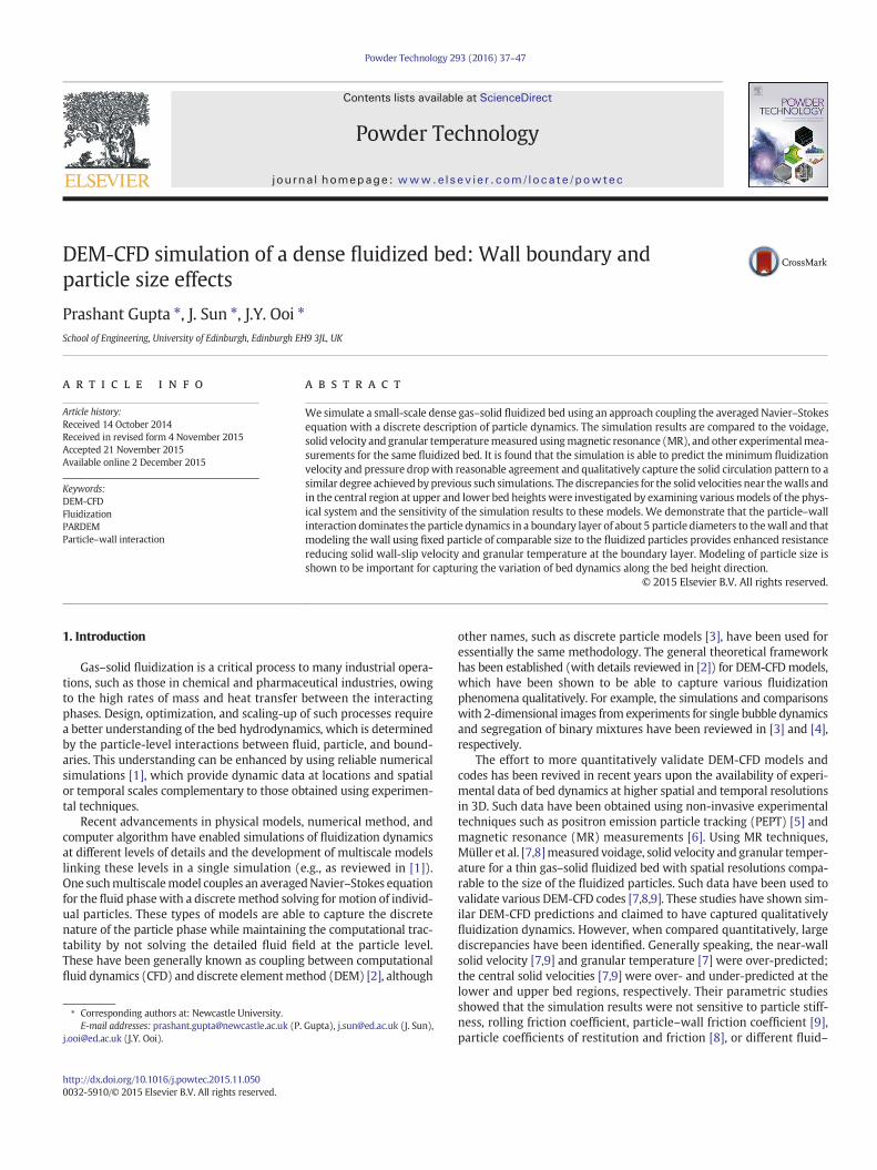
The full-scale bed was simulated with parameters for the geometry,fluid properties, and contact model summarized in Table 1. The fluiddrag on the front and back of the bed is not included in the bed. Thedrag effect was not regarded as critical to the voidage and the averagedparticle velocity profiles in the lateral direction because these quantitieswere measured in the middle planar region of the bed (parallel to thefront and back wall) in the experiments as well as in simulations [8].The distributor plate was simulated using 4 layers of fixed particles of1 mm diameter which covered 2 fluid cells exactly. The particle–wallinteraction was modeled as either with a flat surface or with a wallconsisting of solid particles, whose details will be given in Section 4.3.The no-slip boundary condition was applied between fluid and all thewalls. The coefficient of friction between particles and the walls wasset to 0.1. DEM parameters were suggested by Müller et al. [8] basedon values taken from the literature and employed here as the basecase. A typical snap shot of the DEM-CFD simulation at a superficialvelocity of 0.9 m/s can be seen in Fig. 1(a).
3.2. Post-processing of DEM data
Post-processing of DEM data is important for the correct comparisonbetween the experiment and the simulations. In the experiments, spa-tial–temporal average of theMRdatawas evaluated to obtain the voidage,particle velocity, and granular temperature profiles in the experiments[22]. In order to have a direct comparison between DEM data and MRmeasurement, compatible post-processing techniques should be used.The spatial–temporal averaged solid volume fraction ϕ and velocity V atthe location r are calculated, respectively, using
ϕ rð Þ ¼ π6Nf
∑N f
j¼1∑Np
i¼1d3i W r� ri; j
� �; ð10Þ
and
V rð Þ ¼∑N f
j¼1 ∑Np
i¼1 vi; jW r� ri; j� �
∑N f
j¼1 ∑Np
i¼1 W r� ri; j� � ; ð11Þ
where di , j and vi , j are the diameter and instantaneous velocity of aparticle at a location ri and a time instant j, respectively, Np is thenumber of particles in the domain, Nf is the number of time stepsused in the time averaging, and W(r - ri) is a weighting function.We used WðxÞ ¼ 1
ΩðwÞHðw� jjxjjÞ, where H represents the Heavi-side
function and Ω(w) is the volume of the averaging sphere of radius w.The averaging results were found not sensitive to the forms of theweighting function. However, the results were sensitive to the pa-rameters of the weighting function. The calculation of solid velocityin Eq. (11) is consistent with the so-called “particle based averag-ing” used in [23,24,25], which was found to yield better agreementbetweenDEM and experimental analysis than using the “frame based av-eraging” approach, in which the spatially averaged solid velocity at everytime instant is averaged over time with equal weightings.
Since the MR measurements are time-averaged measurements ofthe mean and variance of the velocity, the MR measured variance ofthe velocity is a combination of both the local fluctuations about themean velocity, and the time-averaged fluctuations of the mean velocity[7]. It is not possible to separate these contributions to granular
Fig. 1.A typical snapshot of DEM–CFD simulation of a gas–solidfluidized bedwith a particle diameter of 1.2mmand density of 1000 kg/m3 at the inlet velocity of 0.9m/s. (a) Base case,flatsidewalls. (b) Simulation domain with particle–wall boundaries.
Fig. 2. Pressure drop (ΔP) across the bed (normalizedwith the bedweight,W divided by bedcross-sectional area, (A) plotted against the fluid inlet velocity (normalized by experimentalminimum fluidization velocity Umf
exp= 0.3 m/s) for different drag models.
40 P. Gupta et al. / Powder Technology 293 (2016) 37–47
temperature in the MR measurements. We calculate the granulartemperature, consistent with that calculated in the experiments [22]as given by
θ rð Þ ¼ 13
V 0xV
0x þ V 0
yV0y þ V 0
zV0z
� �; ð12Þ
where the variance of the velocity ( �V 0iV
0j) is defined as
V 0iV
0j rð Þ ¼ 1
N f∑N f
k¼1Vi;k r; tð Þ � Vi rð Þ� �
V j;k r; tð Þ � V j rð Þ� �: ð13Þ
The spatially averaged velocity Vðr; tÞ is calculated by
V r; tð Þ ¼ ∑Np
i¼1 viW r� rið Þ∑Np
i¼1 W r� rið Þ: ð14Þ
The averaged voidage, solid velocity, and granular temperature aredependent on the spatial and temporal scales used for the averaging.The scales were found to be functions of number of particles, averagingtime, sampling frequency, and dynamics of the system. Studies havebeen carried out to determine the length and time scales at which theresults are approximately invariant to the scales. It was found that alength scale of 2.5 times of particle diameters, a sampling frequency of100 Hz, and an averaging time of 45 s yield such scale invariant results.In order to make the time-averaged DEM results comparable to theexperimental results, the time length used for averaging has beenso determined as to make the averaged results independent of thenumber of instantaneous flow profiles contained. We now turn outattention to the simulation results and the comparison with the ex-perimental results.
4. Results and discussions
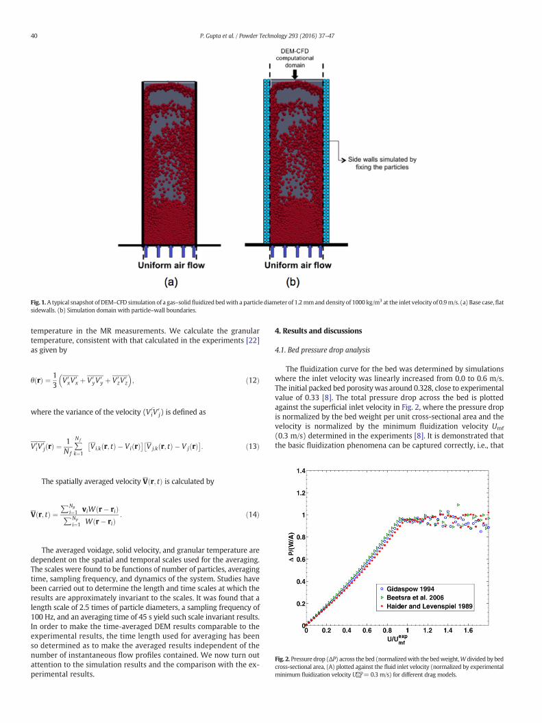
4.1. Bed pressure drop analysis
The fluidization curve for the bed was determined by simulationswhere the inlet velocity was linearly increased from 0.0 to 0.6 m/s.The initial packed bed porosity was around 0.328, close to experimentalvalue of 0.33 [8]. The total pressure drop across the bed is plottedagainst the superficial inlet velocity in Fig. 2, where the pressure dropis normalized by the bed weight per unit cross-sectional area and thevelocity is normalized by the minimum fluidization velocity Umf
(0.3 m/s) determined in the experiments [8]. It is demonstrated thatthe basic fluidization phenomena can be captured correctly, i.e., that
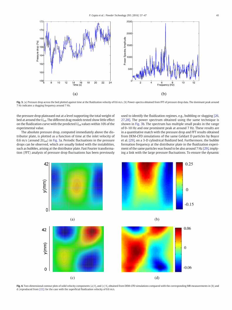
Fig. 3. (a) Pressure drop across the bed plotted against time at the fluidization velocity of 0.6 m/s. (b) Power-spectra obtained from FFT of pressure drop data. The dominant peak around7 Hz indicates a slugging frequency around 7 Hz.
41P. Gupta et al. / Powder Technology 293 (2016) 37–47
the pressure drop plateaued out at a level supporting the total weight ofbed at around theUmf. The different dragmodels tested show little effecton the fluidization curvewith thepredictedUmf valueswithin 10% of theexperimental value.
The absolute pressure drop, computed immediately above the dis-tributor plate, is plotted as a function of time at the inlet velocity of0.6 m/s (around 2Umf) in Fig. 3a. Periodic fluctuations in the pressuredrops can be observed, which are usually linked with the instabilities,such as bubbles, arising at the distributor plate. Fast Fourier transforma-tion (FFT) analysis of pressure drop fluctuations has been previously
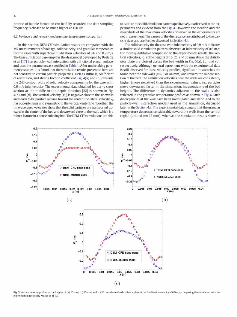
Fig. 4. Two-dimensional contour plots of solid velocity components (a) Vy and (c) Vx obtained frd (reproduced from [22]) for the case with the superficial fluidization velocity of 0.6 m/s.
used to identify the fluidization regimes, e.g., bubbling or slugging [26,27,28]. The power spectrum obtained using the same technique isshown in Fig. 3b. The spectrum has multiple small peaks in the rangeof 0–10 Hz and one prominent peak at around 7 Hz. These results arein a quantitative matchwith the pressure drop and FFT results obtainedfrom DEM-CFD simulations of the same Geldart D particles by Boyceet al. [29], on a 3-D cylindrical fluidized bed. Furthermore, the bubbleformation frequency at the distributor plate in the fluidization experi-ment of the sameparticleswas found to be also around7Hz [29], imply-ing a link with the large pressure fluctuations. To ensure the dynamic
omDEM-CFD simulations comparedwith the correspondingMRmeasurements in (b) and
42 P. Gupta et al. / Powder Technology 293 (2016) 37–47
process of bubble formation can be fully recorded, the data samplingfrequency is chosen to be much higher at 100 Hz.
4.2. Voidage, solid velocity, and granular temperature comparison
In this section, DEM-CFD simulation results are compared with theMR measurements of voidage, solid velocity, and granular temperaturefor the cases with superficial fluidization velocities of 0.6 and 0.9 m/s.The base simulation case employs thedragmodel developed byBeetstraet al. [17], has particle–wall interaction with a frictional planar surface,and uses the parameters as specified in Table 1. After undertaking para-metric studies, it is found that the simulation results presented here arenot sensitive to certain particle properties, such as stiffness, coefficientof restitution, and sliding friction coefficient. Fig. 4(a) and (c) presentsthe 2-D contour plots of solid velocity components for the case with0.6 m/s inlet velocity. The experimental data obtained for a x-–z crosssection at the middle in the depth direction [22] is shown in Fig.4(b) and (d). The vertical velocity (Vy) is negative close to the sidewallsand tends to be positive moving toward the center; the lateral velocity Vxhas opposite signs and symmetric to the vertical centerline. Together, thetime-averaged velocities show that the solid particles are transported up-ward in the center of the bed and downward close to the wall, which is arobust feature in a dense bubbling bed. TheDEM-CFD simulations are able
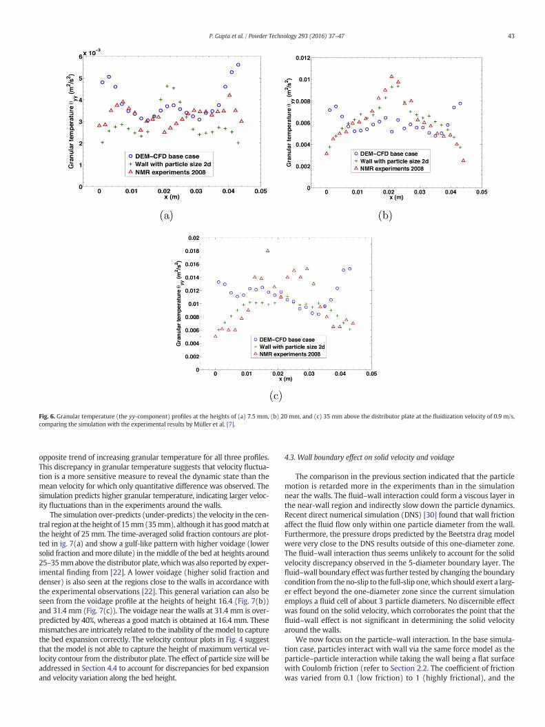
Fig. 5. Vertical velocity profiles at the heights of (a) 15mm, (b) 25mm, and (c) 35mmabove thexperimental results by Müller et al. [7].
to capture this solid circulationpatternqualitatively as observed in the ex-periments and evident from the Fig. 4. However, the location and themagnitude of the maximum velocities observed in the experiments arenot in agreement. The causes of the discrepancy are attributed to the par-ticle sizes and are further discussed in Section 4.4.
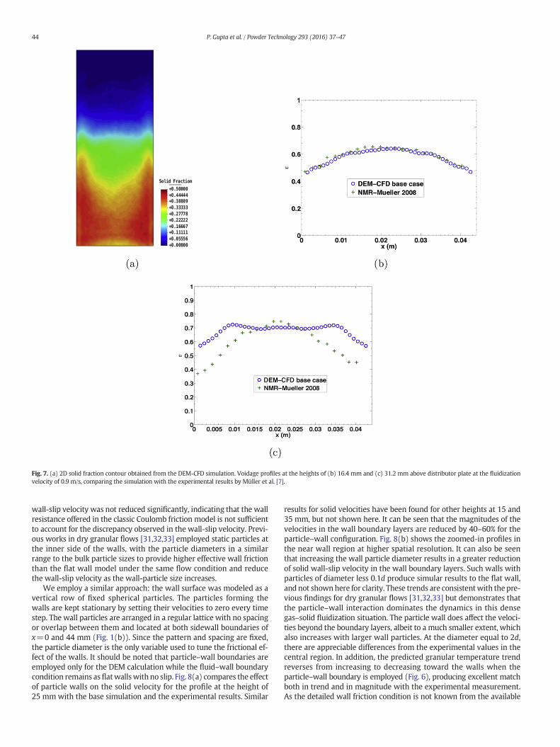
The solid velocity for the case with inlet velocity of 0.9 m/s indicatesa similar solid circulation pattern observed at inlet velocity of 0.6 m/s.For more quantitative comparison to the experimental results, the ver-tical velocities, Vy, at the heights of 15, 25, and 35mm above the distrib-utor plate are plotted across the bed width in Fig. 5(a), (b) and (c),respectively. Although general agreement with the experimental datais still observed for these velocity profiles, significant mismatches arefound near the sidewalls (x=0 or 44 mm) and toward the middle sec-tion of the bed. The simulation velocities near the walls are consistentlyhigher (more negative) than the experimental values, i.e., particlesmove downward faster in the simulation, independently of the bedheights. The difference in dynamics adjacent to the walls is alsoreflected in the granular temperature profiles as shown in Fig. 6. Suchdiscrepancies at the wall have been investigated and attributed to theparticle–wall interaction models used in the simulation, discussedlater in the Section 4.3. The experimental data suggest that the granulartemperature decreases considerably toward the walls from the centralregion (around x=22 mm), whereas the simulation results show an
e distributor plate at the fluidization velocity of 0.9m/s, comparing the simulationwith the
Fig. 6. Granular temperature (the yy-component) profiles at the heights of (a) 7.5 mm, (b) 20 mm, and (c) 35 mm above the distributor plate at the fluidization velocity of 0.9 m/s,comparing the simulation with the experimental results by Müller et al. [7].
43P. Gupta et al. / Powder Technology 293 (2016) 37–47
opposite trend of increasing granular temperature for all three profiles.This discrepancy in granular temperature suggests that velocity fluctua-tion is a more sensitive measure to reveal the dynamic state than themean velocity for which only quantitative difference was observed. Thesimulation predicts higher granular temperature, indicating larger veloc-ity fluctuations than in the experiments around the walls.
The simulation over-predicts (under-predicts) the velocity in the cen-tral region at the height of 15mm(35mm), although it has goodmatch atthe height of 25 mm. The time-averaged solid fraction contours are plot-ted in ig. 7(a) and show a gulf-like pattern with higher voidage (lowersolid fraction andmore dilute) in themiddle of the bed at heights around25–35mmabove the distributor plate, whichwas also reported by exper-imental finding from [22]. A lower voidage (higher solid fraction anddenser) is also seen at the regions close to the walls in accordance withthe experimental observations [22]. This general variation can also beseen from the voidage profile at the heights of height 16.4 (Fig. 7(b))and 31.4 mm (Fig. 7(c)). The voidage near the walls at 31.4 mm is over-predicted by 40%, whereas a good match is obtained at 16.4 mm. Thesemismatches are intricately related to the inability of themodel to capturethe bed expansion correctly. The velocity contour plots in Fig. 4 suggestthat the model is not able to capture the height of maximum vertical ve-locity contour from the distributor plate. The effect of particle size will beaddressed in Section 4.4 to account for discrepancies for bed expansionand velocity variation along the bed height.
4.3. Wall boundary effect on solid velocity and voidage
The comparison in the previous section indicated that the particlemotion is retarded more in the experiments than in the simulationnear the walls. The fluid–wall interaction could form a viscous layer inthe near-wall region and indirectly slow down the particle dynamics.Recent direct numerical simulation (DNS) [30] found that wall frictionaffect the fluid flow only within one particle diameter from the wall.Furthermore, the pressure drops predicted by the Beetstra drag modelwere very close to the DNS results outside of this one-diameter zone.The fluid–wall interaction thus seems unlikely to account for the solidvelocity discrepancy observed in the 5-diameter boundary layer. Thefluid–wall boundary effectwas further tested by changing the boundarycondition from the no-slip to the full-slip one,which should exert a larg-er effect beyond the one-diameter zone since the current simulationemploys a fluid cell of about 3 particle diameters. No discernible effectwas found on the solid velocity, which corroborates the point that thefluid–wall effect is not significant in determining the solid velocityaround the walls.
We now focus on the particle–wall interaction. In the base simula-tion case, particles interact with wall via the same force model as theparticle–particle interaction while taking the wall being a flat surfacewith Coulomb friction (refer to Section 2.2. The coefficient of frictionwas varied from 0.1 (low friction) to 1 (highly frictional), and the
Fig. 7. (a) 2D solid fraction contour obtained from the DEM-CFD simulation. Voidage profiles at the heights of (b) 16.4 mm and (c) 31.2 mm above distributor plate at the fluidizationvelocity of 0.9 m/s, comparing the simulation with the experimental results by Müller et al. [7].
44 P. Gupta et al. / Powder Technology 293 (2016) 37–47
wall-slip velocity was not reduced significantly, indicating that the wallresistance offered in the classic Coulomb friction model is not sufficientto account for the discrepancy observed in the wall-slip velocity. Previ-ous works in dry granular flows [31,32,33] employed static particles atthe inner side of the walls, with the particle diameters in a similarrange to the bulk particle sizes to provide higher effective wall frictionthan the flat wall model under the same flow condition and reducethe wall-slip velocity as the wall-particle size increases.
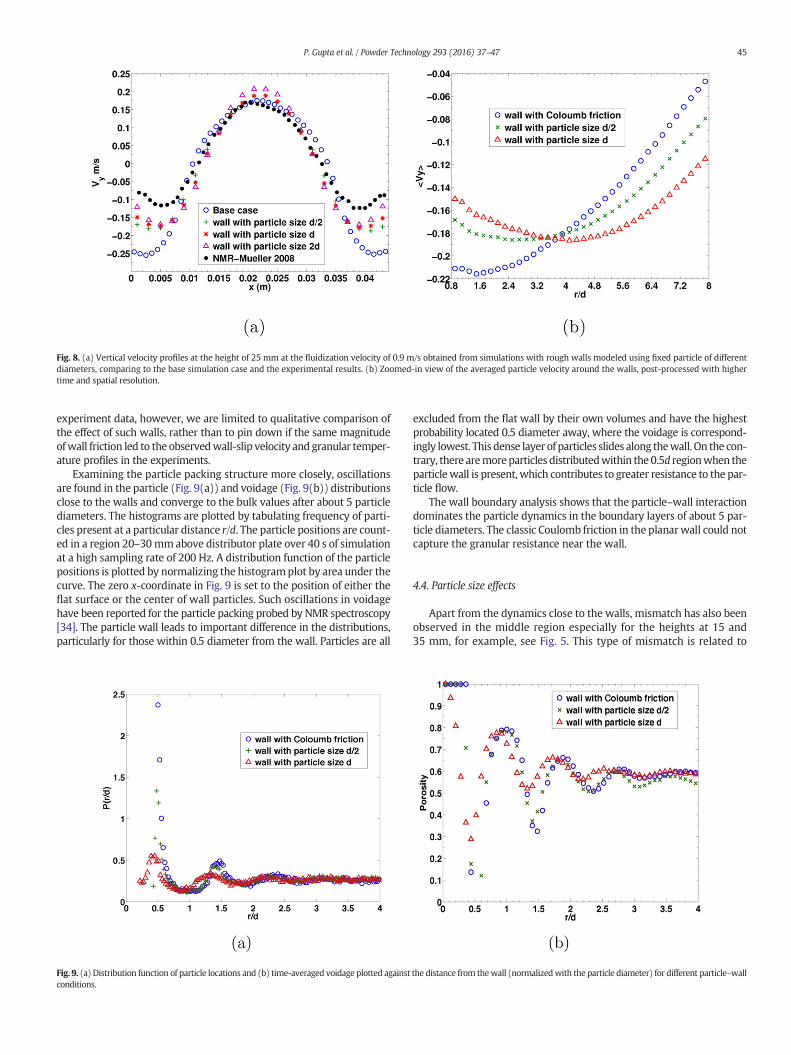
We employ a similar approach: the wall surface was modeled as avertical row of fixed spherical particles. The particles forming thewalls are kept stationary by setting their velocities to zero every timestep. The wall particles are arranged in a regular lattice with no spacingor overlap between them and located at both sidewall boundaries ofx=0 and 44 mm (Fig. 1(b)). Since the pattern and spacing are fixed,the particle diameter is the only variable used to tune the frictional ef-fect of the walls. It should be noted that particle–wall boundaries areemployed only for the DEM calculation while the fluid–wall boundarycondition remains asflatwallswith no slip. Fig. 8(a) compares the effectof particle walls on the solid velocity for the profile at the height of25 mm with the base simulation and the experimental results. Similar
results for solid velocities have been found for other heights at 15 and35 mm, but not shown here. It can be seen that the magnitudes of thevelocities in the wall boundary layers are reduced by 40–60% for theparticle–wall configuration. Fig. 8(b) shows the zoomed-in profiles inthe near wall region at higher spatial resolution. It can also be seenthat increasing the wall particle diameter results in a greater reductionof solid wall-slip velocity in the wall boundary layers. Such walls withparticles of diameter less 0.1d produce simular results to the flat wall,and not shownhere for clarity. These trends are consistentwith the pre-vious findings for dry granular flows [31,32,33] but demonstrates thatthe particle–wall interaction dominates the dynamics in this densegas–solid fluidization situation. The particle wall does affect the veloci-ties beyond the boundary layers, albeit to a much smaller extent, whichalso increases with larger wall particles. At the diameter equal to 2d,there are appreciable differences from the experimental values in thecentral region. In addition, the predicted granular temperature trendreverses from increasing to decreasing toward the walls when theparticle–wall boundary is employed (Fig. 6), producing excellent matchboth in trend and in magnitude with the experimental measurement.As the detailed wall friction condition is not known from the available
Fig. 8. (a) Vertical velocity profiles at the height of 25 mm at the fluidization velocity of 0.9 m/s obtained from simulations with rough walls modeled using fixed particle of differentdiameters, comparing to the base simulation case and the experimental results. (b) Zoomed-in view of the averaged particle velocity around the walls, post-processed with highertime and spatial resolution.
45P. Gupta et al. / Powder Technology 293 (2016) 37–47
experiment data, however, we are limited to qualitative comparison ofthe effect of such walls, rather than to pin down if the same magnitudeofwall friction led to the observedwall-slip velocity and granular temper-ature profiles in the experiments.
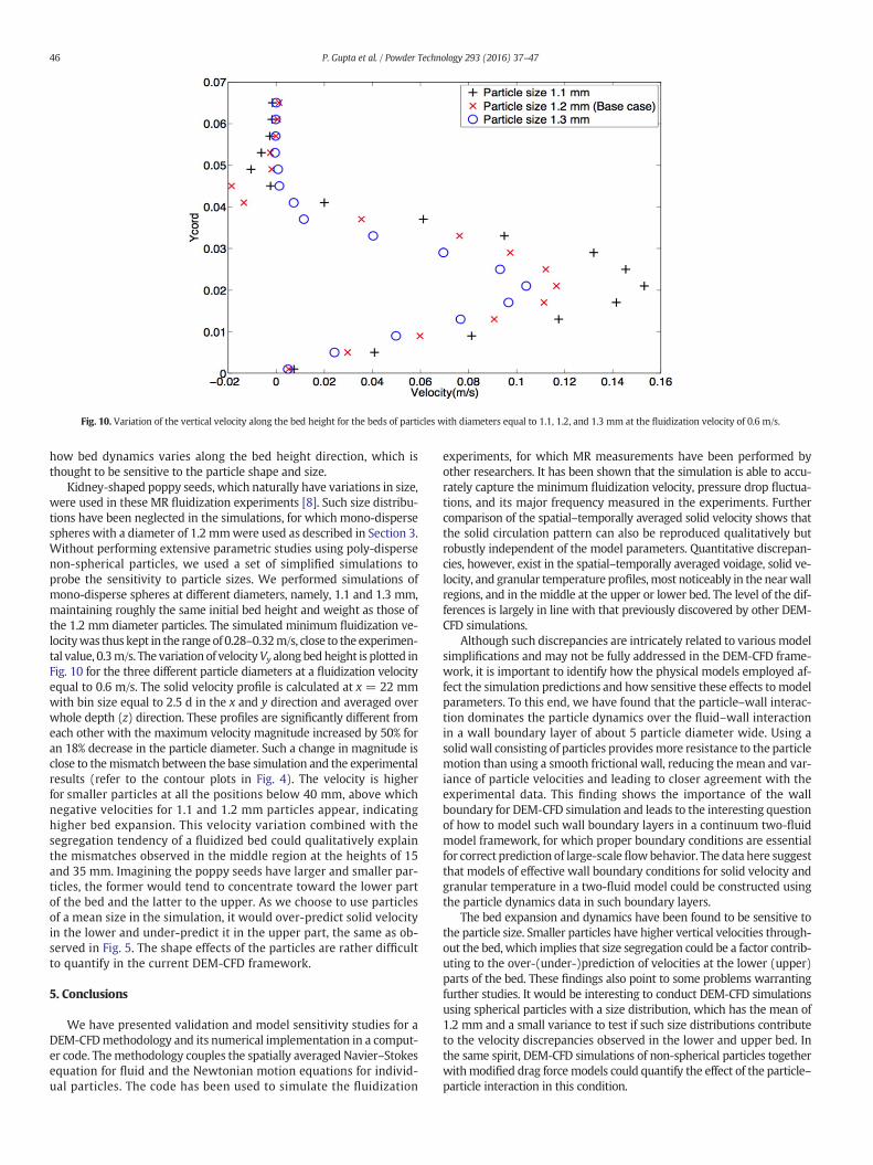
Examining the particle packing structure more closely, oscillationsare found in the particle (Fig. 9(a)) and voidage (Fig. 9(b)) distributionsclose to the walls and converge to the bulk values after about 5 particlediameters. The histograms are plotted by tabulating frequency of parti-cles present at a particular distance r/d. The particle positions are count-ed in a region 20–30mmabove distributor plate over 40 s of simulationat a high sampling rate of 200 Hz. A distribution function of the particlepositions is plotted by normalizing the histogramplot by area under thecurve. The zero x-coordinate in Fig. 9 is set to the position of either theflat surface or the center of wall particles. Such oscillations in voidagehave been reported for the particle packing probed by NMR spectroscopy[34]. The particle wall leads to important difference in the distributions,particularly for those within 0.5 diameter from the wall. Particles are all
Fig. 9. (a) Distribution function of particle locations and (b) time-averaged voidage plotted againstconditions.
excluded from the flat wall by their own volumes and have the highestprobability located 0.5 diameter away, where the voidage is correspond-ingly lowest. This dense layer of particles slides along thewall. On the con-trary, there aremoreparticles distributedwithin the0.5d regionwhen theparticlewall is present, which contributes to greater resistance to the par-ticle flow.
The wall boundary analysis shows that the particle–wall interactiondominates the particle dynamics in the boundary layers of about 5 par-ticle diameters. The classic Coulomb friction in the planarwall could notcapture the granular resistance near the wall.
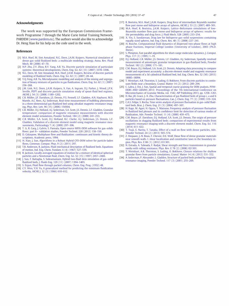
4.4. Particle size effects
Apart from the dynamics close to the walls, mismatch has also beenobserved in the middle region especially for the heights at 15 and35 mm, for example, see Fig. 5. This type of mismatch is related to
the distance from thewall (normalizedwith the particle diameter) for different particle–wall
Fig. 10. Variation of the vertical velocity along the bed height for the beds of particles with diameters equal to 1.1, 1.2, and 1.3 mm at the fluidization velocity of 0.6 m/s.
46 P. Gupta et al. / Powder Technology 293 (2016) 37–47
how bed dynamics varies along the bed height direction, which isthought to be sensitive to the particle shape and size.
Kidney-shaped poppy seeds, which naturally have variations in size,were used in these MR fluidization experiments [8]. Such size distribu-tions have been neglected in the simulations, for which mono-dispersespheres with a diameter of 1.2 mmwere used as described in Section 3.Without performing extensive parametric studies using poly-dispersenon-spherical particles, we used a set of simplified simulations toprobe the sensitivity to particle sizes. We performed simulations ofmono-disperse spheres at different diameters, namely, 1.1 and 1.3 mm,maintaining roughly the same initial bed height and weight as those ofthe 1.2 mm diameter particles. The simulated minimum fluidization ve-locitywas thus kept in the rangeof 0.28–0.32m/s, close to the experimen-tal value, 0.3m/s. The variation of velocityVy along bedheight is plotted inFig. 10 for the three different particle diameters at a fluidization velocityequal to 0.6 m/s. The solid velocity profile is calculated at x = 22 mmwith bin size equal to 2.5 d in the x and y direction and averaged overwhole depth (z) direction. These profiles are significantly different fromeach other with the maximum velocity magnitude increased by 50% foran 18% decrease in the particle diameter. Such a change in magnitude isclose to themismatch between the base simulation and the experimentalresults (refer to the contour plots in Fig. 4). The velocity is higherfor smaller particles at all the positions below 40 mm, above whichnegative velocities for 1.1 and 1.2 mm particles appear, indicatinghigher bed expansion. This velocity variation combined with thesegregation tendency of a fluidized bed could qualitatively explainthe mismatches observed in the middle region at the heights of 15and 35 mm. Imagining the poppy seeds have larger and smaller par-ticles, the former would tend to concentrate toward the lower partof the bed and the latter to the upper. As we choose to use particlesof a mean size in the simulation, it would over-predict solid velocityin the lower and under-predict it in the upper part, the same as ob-served in Fig. 5. The shape effects of the particles are rather difficultto quantify in the current DEM-CFD framework.
5. Conclusions
We have presented validation and model sensitivity studies for aDEM-CFDmethodology and its numerical implementation in a comput-er code. Themethodology couples the spatially averaged Navier–Stokesequation for fluid and the Newtonian motion equations for individ-ual particles. The code has been used to simulate the fluidization
experiments, for which MR measurements have been performed byother researchers. It has been shown that the simulation is able to accu-rately capture the minimum fluidization velocity, pressure drop fluctua-tions, and its major frequency measured in the experiments. Furthercomparison of the spatial–temporally averaged solid velocity shows thatthe solid circulation pattern can also be reproduced qualitatively butrobustly independent of the model parameters. Quantitative discrepan-cies, however, exist in the spatial–temporally averaged voidage, solid ve-locity, and granular temperature profiles,most noticeably in the nearwallregions, and in the middle at the upper or lower bed. The level of the dif-ferences is largely in line with that previously discovered by other DEM-CFD simulations.
Although such discrepancies are intricately related to various modelsimplifications and may not be fully addressed in the DEM-CFD frame-work, it is important to identify how the physical models employed af-fect the simulation predictions and how sensitive these effects to modelparameters. To this end, we have found that the particle–wall interac-tion dominates the particle dynamics over the fluid–wall interactionin a wall boundary layer of about 5 particle diameter wide. Using asolidwall consisting of particles providesmore resistance to the particlemotion than using a smooth frictional wall, reducing themean and var-iance of particle velocities and leading to closer agreement with theexperimental data. This finding shows the importance of the wallboundary for DEM-CFD simulation and leads to the interesting questionof how to model such wall boundary layers in a continuum two-fluidmodel framework, for which proper boundary conditions are essentialfor correct prediction of large-scale flowbehavior. The data here suggestthat models of effective wall boundary conditions for solid velocity andgranular temperature in a two-fluid model could be constructed usingthe particle dynamics data in such boundary layers.
The bed expansion and dynamics have been found to be sensitive tothe particle size. Smaller particles have higher vertical velocities through-out the bed, which implies that size segregation could be a factor contrib-uting to the over-(under-)prediction of velocities at the lower (upper)parts of the bed. These findings also point to some problems warrantingfurther studies. It would be interesting to conduct DEM-CFD simulationsusing spherical particles with a size distribution, which has the mean of1.2 mm and a small variance to test if such size distributions contributeto the velocity discrepancies observed in the lower and upper bed. Inthe same spirit, DEM-CFD simulations of non-spherical particles togetherwithmodified drag forcemodels could quantify the effect of the particle–particle interaction in this condition.
47P. Gupta et al. / Powder Technology 293 (2016) 37–47
Acknowledgments
The work was supported by the European Commission Frame-work Programme 7 through the Marie Curie Initial Training Network,PARDEM (www.pardem.eu). The authorswould also like to acknowledgeDr. Heng Xiao for his help on the code used in the work.
References
[1] M.A. Hoef, M. Sint Annaland, N.G. Deen, J.A.M. Kuipers, Numerical simulation ofdense gas–solid fluidized beds: a multiscale modeling strategy, Annu. Rev. FluidMech. 40 (2008) 47–70.
[3] N.G. Deen, M. Sint Annaland, M.A. Hoef, J.A.M. Kuipers, Review of discrete particlemodeling of fluidized beds, Chem. Eng. Sci. 62 (1) (2007) 28–44.
[4] Y.Q. Feng, A.B. Yu, Microdynamic modelling and analysis of the mixing and segrega-tion of binary mixtures of particles in gas fluidization, Chem. Eng. Sci. 62 (1) (2007)256–268.
[5] J.M. Link, N.G. Deen, J.A.M. Kuipers, X. Fan, A. Ingram, D.J. Parker, J. Wood, J.P.K.Seville, PEPT and discrete particle simulation study of spout-fluid bed regimes,AICHE J. 54 (5) (2008) 1189–1202.
[6] C.R. Müller, J.F. Davidson, J.S. Dennis, P.S. Fennell, L.F. Gladden, A.N. Hayhurst, M.D.Mantle, A.C. Rees, A.J. Sederman, Real-time measurement of bubbling phenomenain a three-dimensional gas-fluidized bed using ultrafast magnetic resonance imag-ing, Phys. Rev. Lett. 96 (15) (2006) 154504.
[7] C.R. Müller, D.J. Holland, A.J. Sederman, S.A. Scott, J.S. Dennis, L.F. Gladden, Granulartemperature: comparison of magnetic resonance measurements with discreteelement model simulations, Powder Technol. 184 (2) (2008) 241–253.
[8] C.R. Müller, S.A. Scott, D.J. Holland, B.C. Clarke, A.J. Sederman, J.S. Dennis, L.F.Gladden, Validation of a discrete element model using magnetic resonance mea-surements, Particuology 7 (4) (2009) 297–306.
[9] T. Li, R. Garg, J. Galvin, S. Pannala, Open-source MFIX-DEM software for gas–solidsflows: part II— validation studies, Powder Technol. 220 (2012) 138–150.
[10] D. Gidaspow, Multiphase flow and fluidization: continuum and kinetic theory de-scriptions, Academic press, 1994.
[11] H. Xiao, J. Sun, Algorithms in a Robust Hybrid CFD-DEM solver for particle-ladenflows, Commun. Comput. Phys. 9 (2) (2011) 297.
[13] R. Jackson, Locally averaged equations of motion for a mixture of identical sphericalparticles and a Newtonian fluid, Chem. Eng. Sci. 52 (15) (1997) 2457–2469.
[14] J. Sun, F. Battaglia, S. Subramaniam, Hybrid two-fluid dem simulation of gas–solidfluidized beds, J. Fluids Eng. 129 (11) (2007) 1394–1403.
[15] S. Ergun, Fluid flow through packed columns, Chem. Eng. Prog. (1952) 48.[16] C.Y. Wen, Y.H. Yu, A generalized method for predicting the minimum fluidization
velocity, AICHE J. 12 (3) (1966) 610–612.
[17] R. Beetstra, M.A. Hoef, J.A.M. Kuipers, Drag force of intermediate Reynolds numberflow past mono-and bidisperse arrays of spheres, AICHE J. 53 (2) (2007) 489–501.
[18] M.A. Hoef, R. Beetstra, J.A.M. Kuipers, Lattice–Boltzmann simulations of low-Reynolds-number flow past mono-and bidisperse arrays of spheres: results forthe permeability and drag force, J. Fluid Mech. 528 (2005) 233–254.
[19] X. Yin, S. Sundaresan, Drag law for bidisperse gas–solid suspensions containingequally sized spheres, Ind. Eng. Chem. Res. 48 (1) (2008) 227–241.
[20] H. Rusche, Computational fluid dynamics of dispersed two-phase flows at highphase fractions, Imperial College London (University of London), 2003 (Ph.D.thesis).
[21] S. Plimpton, Fast parallel algorithms for short-range molecular dynamics, J. Comput.Phys. 117 (1) (1995) 1–19.
[22] D.J. Holland, C.R. Müller, J.S. Dennis, L.F. Gladden, A.J. Sederman, Spatially resolvedmeasurement of anisotropic granular temperature in gas-fluidized beds, PowderTechnol. 182 (2) (2008) 171–181.
[23] C.M. Boyce, D.J. Holland, S.A. Scott, J.S. Dennis, Adapting data processing to comparemodel and experiment accurately: a discrete element model and magnetic resonancemeasurements of a 3d cylindrical fluidized bed, Ind. Eng. Chem. Res. 52 (50) (2013)18085–18094.
[24] T. Weinhart, A.R. Thornton, S. Luding, O. Bokhove, From discrete particles to contin-uum fields near a boundary, Granul. Matter 14 (2) (2012) 289–294.
[25] C. Labra, J. Ooi, J. Sun, Spatial and temporal coarse-graining for DEM analysis, POW-DERS AND GRAINS 2013: Proceedings of the 7th International Conference onMicromechanics of Granular Media, vol. 1542, AIP Publishing 2013, pp. 1258–1261.
[26] D. Bai, J.R. Grace, J.-X. Zhu, Characterization of gas fluidized beds of group c, a and bparticles based on pressure fluctuations, Can. J. Chem. Eng. 77 (2) (1999) 319–324.
[27] C.A.S. Felipe, S. Rocha, Time series analysis of pressure fluctuation in gas–solid fluid-ized beds, Braz. J. Chem. Eng. 21 (3) (2004) 497–507.
[28] H. Kage, M. Agari, H. Ogura, Y. Matsuno, Frequency analysis of pressure fluctuationin fluidized bed plenum and its confidence limit for detection of various modes offluidization, Adv. Powder Technol. 11 (4) (2000) 459–475.
[29] C.M. Boyce, J.F. Davidson, D.J. Holland, S.A. Scott, J.S. Dennis, The origin of pressureoscillations in slugging fluidized beds: comparison of experimental results frommagnetic resonance imaging with a discrete element model, Chem. Eng. Sci. 116(2014) 611–622.
[30] T. Tsuji, E. Narita, T. Tanaka, Effect of a wall on flow with dense particles, Adv.Powder Technol. 24 (2) (2013) 565–574.
[31] Z. Shojaaee, J.-N. Roux, F. Chevoir, D.E. Wolf, Shear flow of dense granular materialsnear smooth walls. I. shear localization and constitutive laws in the boundary re-gion, Phys. Rev. E 86 (1) (2012) 011301.
[32] N. Estrada, A. Taboada, F. Radjai, Shear strength and force transmission in granularmedia with rolling resistance, Phys. Rev. E 78 (2) (2008) 021301.
[33] T. Weinhart, A.R. Thornton, S. Luding, O. Bokhove, Closure relations for shallowgranular flows from particle simulations, Granul. Matter 14 (4) (2012) 531–552.
[34] A. Sederman, P. Alexander, L. Gladden, Structure of packed beds probed bymagneticresonance imaging, Powder Technol. 117 (3) (2001) 255–269.