1

Demand Assessment and Price-Elasticity Estimation of Quality-Improved Primary Health Care in Palestine: Some Responses from the Contingent Valuation Method.* Awad Matariaa,b, Stéphane Luchinic, and Jean-Paul Moattia,c,d

a INSERM U379 / ORS, Marseille - France b Institute of Community and Public Health, Birzeit University, Palestine c GREQAM-CNRS, Institute of Public Economics (IDEP), Marseille - France d University of the Mediterranean, Marseille – France The paper proposes a new methodology to assess demand and estimate price-elasticity for health care, based on patients’ stated willingness to pay (WTP) values for certain aspects of quality improvements. A conceptual analysis of how respondents consider contingent valuation (CV) questions permits us to specify a probability density function for sated WTP values; and consequently, to model a demand function for quality-improved health care. The model was empirically estimated using a CV study intended to assess patients’ values for improving the quality of primary health care in Palestine. Quality was apprehended using a multi-attribute approach; and respondents valued specified quality improvements using a decomposed valuation scenario and a payment card elicitation technique. A Random sample of 499 individuals were interviewed; most (91.8%) declared willing to pay extra user fees to benefit from better quality. Demand analysis suggests an inelastic demand at low user fees; and when price-increase is accompanied by important quality-improvements. Nevertheless, demand becomes more and more elastic if user fees continue to rise. On the other hand, patients’ reaction to price-increase turns out to be dependent on one’s income. Our results can be used to elaborate successful health care financial strategies while respecting individuals’ own preferences and financial capacities. Keywords: willingness to pay, contingent valuation, cost-sharing, demand, price-elasticity, Weibull distribution, Palestine

1. Introduction: Predicting patients’ reaction to changes in medical services’ prices represents one of the more challenging tasks confronting developing countries’ policymakers in elaborating successful health care financial strategies. During the last two decades and adhering to some international organizations’ recommendations; e.g., World Bank and WHO, many developing countries envisaged and started to implement cost-sharing policies (World-Bank 1987). This consists of attributing a user fee (price) to medical services to be paid by the users at the point of consumption (McPake, Hanson et al. 1993); which shall promote, at least in theory, improving the quality of delivered care (Dumoulin 1993). Pricing decisions are often difficult for health care providers who fear that increased fees will cripple demand and create barriers to access for poor clients. Therefore, contrary to other economic contents where prices are usually set to maximize profitability, health care policy makers should compromise between accessibility and sustainability goals (Foreit and Foreit 2003). The solution for this dilemma shall start by a proper characterization of the demand function for health care, and by an accurate estimation of demand price- and income-elasticities. Cissé et al. (Cissé, Luchini et al. 2002) in a recent literature review of health care demand studies highlighted many conceptual and empirical gaps in our knowledge in this area. Most studies attempting to assess health care demand and to estimate price-elasticity leaned on observations about individuals’ behaviors during recent or current health problems (Gertler and Hammer 1997). Different econometric models were used to specify the quantity demanded (number of visits), or the probability to demand a certain type of care (primary health care PHC, private clinic, hospital, auto-medication, etc.) as a function of services’ prices and quality levels - adjusting for users’ own characteristics including one’s income (Cissé, Luchini et al. 2002). Most of these studies used cross-sectional household surveys to model the relationship between price and demand; e.g., Mwabu et al. study in Kenya (Mwabu, Ainsworth et al. 1993); some considered demand fluctuation following variations in prices practiced by the health care providers (Waddington and Enyimayew 1990); others used experimental design techniques to randomly attribute different pricing strategies to different health centers (Gertler and Molyneaux 1997; Bratt, Weaver et al. 2002), or to randomly assign individuals to different health plans with different payment structures (Newhouse 1995). The common

* Corresponding author : Awad Mataria, INSERM U379 / ORS, 23 rue Stanislas Torrents, 13006 Marseille, France. Tel: +33 4 96 17 60 78; Fax: +33 4 96 17 60 73; e-mail: awad@birzeit.edu

2

feature in all of these studies is their reliance on comparisons of patients’ reactions to different economic environments using patients’ real economic behaviors. On the other hand, a limited number of studies used stated preference techniques to elicit patients’ behavior vis-à-vis different pricing strategies (Abel-Smith and Rawal 1992; Weaver, Ndamobissi et al. 1996; Gyldmark and Morrison 2001; Onwujekwe, Chima et al. 2001; Onwujekwe, Chima et al. 2002; Whittington, Matsui-Santana et al. 2002; Foreit and Foreit 2003). These studies were designed to assess patients’ WTP values for certain types of health care or for certain aspects of quality improvements using contingent valuation methodology. Their common objective - which was highly implicit in most of the cases - was to apprehend the underlying health care demand function. The authors in these studies had either analyzed the determinants of patients’ stated WTP values (Weaver, Ndamobissi et al. 1996; Gyldmark and Morrison 2001; Onwujekwe, Chima et al. 2001; Onwujekwe, Chima et al. 2002), or used simple descriptive analysis to sketch the demand curve for quality-improved health care1 (Whittington, Matsui-Santana et al. 2002; Foreit and Foreit 2003). Contingent valuation (CV), as it has been defined by Klose (Klose 1999), is a direct hypothetical survey technique used to assess the maximum amount of money the respondent is willing to pay for the commodity in question; i.e., its value. From a microeconomic perspective, this shall represent the height of the inversed-demand curve for the commodity in question (Varian 2000). In this paper we consider WTP data from a “different” angle, attempting to exhaust most of the information embedded in individuals’ stated monetary values, to model - in a “highly” flexible way - the demand function for quality-improved medical care, and to estimate demand price-elasticity. The spirit of our suggestion emerges from a dynamic psychometric analysis of the decision making process by which the respondent states her/his maximum WTP value for the commodity in question following an open-ended elicitation technique supported by a payment card2. The empirical part of the paper concerns a CV study carried out to assess patients’ WTP values for improving different aspects of quality of PHC services in Palestine. The paper research methodology is developed in the second section where we argue the underlying theoretical model and present the CV questionnaire instrument. Section three includes the econometric analysis and demand function specification. Estimation results are presented and discussed in section four and five. In the sixth section, we conclude by some recommendations and propositions for future research.

2. Materials and methods: a. Theoretical model:

Our framework is a model on which utility depends on health and on the consumption of goods other than medical care. If an illness is experienced, individuals decide whether or not to seek medical care based on the benefits and costs of the latter. The benefits from consuming medical care is an improvement in health; and the cost of seeking medical care is a reduction in the consumption of other goods. Formally, let the expected utility of individual i following medical care be given by:

Ui (Hi , Ci) with ∂Ui/∂Hi >0 and ∂Ui/∂Ci > 0 (1) where Hi is individual i’s expected health status following medical consultation; and Ci is the consumption net of the cost of obtaining care. The purchased medical care is invested in health and the expected improvement in health depends upon: the quality of delivered care Qi and a vector of individual characteristics Xi (e.g., health status and education). Given that, we are interested in individual’s own price/quality tradeoffs, the second argument (Xi) can be excluded from the health production function. The quality of the service is an intrinsic characteristic over which the individual has no influence; nevertheless, it is the perceived quality that counts in a price/quality tradeoff decision - this might vary from one individual to another. The consumption expenditures Ci are derived from the budget constraint. If UFi is the user fee (price)

1 Some authors sketched the demand curve as the % of respondents having a WTP value ≥ a given use fee versus service’s price, with the possibility to stratify the sample on key independent variables; e.g., sex, to conduct within-sample comparisons. 2 The conceptual analysis in this paper could be generalized to certain forms of bidding game elicitation techniques.

3

that individual i has to pay to get the medical service and Yi is individual i’s income, the budget constraint can be written as follows:

UFi + Ci = Yi (2) Substituting in (1) yields the following indirect utility function: Ui = Ui (Hi(Qi) , Yi – UFi) (3) Let us consider two quality levels, each associated with a certain user fee payment: QiA is the status quo quality level as it is perceived by individual i; and QiB is the improved quality level as it is perceived by individual i. UFiA is the current user fee as it is paid by individual i; and UFiB is the new proposed user fee following the quality improvement. Using equation (3) we can write the expected utility of individual i conditional on the medical consultation in the status quo and in the new proposed situations. These are, UiA = Ui (Hi(QiA) , Yi – UFiA) and UiB = Ui (Hi(QiB) , Yi – UFiB) (4) The demand function for the quality-improved medical service Di (.) is specified as a discrete demand function as follows:

Di = 1 if individual i demands the service (given quality being improved) Di = 0 otherwise.

Individual i demands the service if and only if UiB ≥ UiA ; i.e., ∆Ui ≥ 0. This implies that Di = 1 if and only if: UmQi (QAi)*dQi + UmCi (CAi) * dCi ≥ 03 i.e., [UmQi (QAi) / UmCi (CAi)] * dQi ≥ - dCi (5) where Um is the marginal utility function with respect to each of the arguments; QiB = QiA + dQi and CiB = CiA + dCi The left-hand side of the inequality in (5) contains a ratio of two marginal utilities which is an estimation of the marginal rate of substitution (MRS) between Qi and Ci. The MRS represents the amount of Ci that individual i would be prepared to give up in order to have an extra unit of Qi. Since Ci in our model is measured in monetary units, the MRS shall represent the amount of money individual i would be willing to pay for a unit increase in Qi. Multiplying the MRS by the amplitude of quality improvement dQi (in equation 5) gives an estimation of individual i’s WTP value for a quality improvement of magnitude dQi. Substituting in (5) gives:

MRSC/Q * dQi ≥ - dCi ⇒ WTP i ≥ - dCi ⇒ WTP i ≥ ∆UFi4 (6)

This represents the general condition to demand the quality-improved service if the improvement was accompanied with a User Fee Increment of UFIi (UFI = ∆UF); i.e., WTP i ≥ UFIi (7) This means that individual i would continue to demand the quality-improved service even if she/he has to pay an extra user fee for it, as long as, the user fee increment does not go beyond her/his WTP for the improvement itself. In our study, a quality improvement from QiA to QiB is proposed to the individual. The latter is asked using the payment card elicitation technique to select the highest extra user fee she/he would be willing to pay given the improvement. Each respondent considered a list of continuous increments in the user fee; starting from 0, 1, 2, … and up to 10 NIS5 (respondents specified the value if it was greater than 10 NIS). For each amount, the respondent compares her/his maximum WTP for the improvement - a value that she/he has in mind - with the proposed user fee increment UFI. In the end,

3 Here, the health production function is substituted by the perceived quality level since the latter is assumed to be the only variable influencing the ex-post health status. 4 dCi is the difference in consumption due to user fee increase:

dCi = CiB - CiA = (Yi – UFiB) – (Yi – UFiA) = UFiA – UFiB = -∆UFi. 5 At the moment of the study 1 New Israel Shekel (NIS) was equivalent to 0.24 US$.

4

she/he declares the highest increment that she/he would be prepared to accept (her/his WTP). This value also represents the increment beyond which the consumer quits the pool of the demanders of the improved service. In other words, if UFIi > WTPi, individual i would prefer not to demand the service. To present this in a more formal way, we assume that the WTP value is a continuous random variable with probability density function PDF: f(WTP) providing the “probability” that the individual has a WTP value of a given UFI. Based on the PDF we can define the cumulative density function CDF of WTP which represents the probability that individual i has a WTP value less than or equal a given UFI. The CDF is specified as follows:

CDF (WTP) = Pr {WTP ≤ UFI} = ∫UFI

0

Pf(WTP).dWT (8)

In other words, and noting that the individual is considering continuous gradual increments in the user fee, the CDF represents the probability that the individual ceases to demand the service by a user fee increment of UFI. Consequently, the demand function is represented by the complement of the CDF - also called the De-Cumulative Distribution Function. Sketching the demand curve as one minus the CDF for the WTP responses has been alluded to by Mitchell and Carson (1989, p48) (Mitchell and Carson 1989). Hence, the demand function is specified as follows:

D(UFI) = Pr {WTP > UFI} = 1 – CDF(WTP) = ∫∞

UFI

Pf(WTP).dWT (9)

This gives the probability that the service continues to be demanded by the user at a user fee increment of UFI; or more generally, it gives the probability that the respondent does not stop to demand the service following an extra user fee of UFI (of course, given that quality is being improved). Explanatory variables including, the amplitude of quality improvement (dQi), individual demographic and socio-economic characteristics (including income), and center's characteristics, can be included in the formula of PDF and thus CDF to incorporate additional determinants of the corresponding probability and to generalize the PDF. Thus, we can write the demand function for a medical service following quality improvement and user fee increment as follows:

)X , dQ , (UFI D | service thedemand y toProbabilit (.) D UFI,dQ iiii i == (10) One should notice the similarities between the above model and duration models used by economists to empirically study time based events like unemployment spills; and those used by epidemiologists to conduct survival analysis. In our model, time is replaced by user fee increment (price); and the survival function is transformed to a demand function.

b. Contingent valuation: A CV questionnaire was prepared, tested and administered by pre-trained interviewers on a random sample of patients seeking care in four PHC centers situated in Ramallah district (Palestine). Two of them are governmental and the other two are private-not-for profit non-governmental PHC centers (NGO); on the other hand, two of the centers are urban and two are rural. Any patient getting out from the medical consultation was eligible to take part in our study. Following some introductory information on CV, in general, and on its use in our study, respondents were requested to value specified amplitudes of quality improvements over seven pre-selected quality attributes (see Appendix A for the selected attributes and their corresponding measurement scales). For this purpose, respondents were asked to characterize the current status of each of the quality attributes, as they perceive them; and then to assess a transition from the status quo to the “best” state of each attribute, i.e., to state their maximum WTP for the specified improvements. Respondents perceive the status quo level of each attribute differently; however, the “best” proposed state for each attribute was the same for all the respondents (a “Very Close” PHC center, a “Not Long at All” waiting time, etc.). This implies that different respondents value different amplitudes of quality improvements, depending on their own current situations. Improvements over each attribute were assessed separately using a decomposed valuation scenario (O'Brien and Gafni 1996); and values were revealed using a payment card elicitation technique (Mitchell and Carson 1989; Donaldson, Thomas et al. 1997) [see Appendix

5

B for a summary of the valuation process including WTP questions]. In the last section, individual demographic and socio-economic characteristics were collected. For more details on questionnaire elaboration and validity testing of stated WTP values, including, construct and internal validity, see Mataria et al. (Mataria, Donaldson et al. 2002).

3. Econometric analysis: The critical step in modeling the demand function based on the above conceptual analysis is to properly specify the WTP PDF. This is based on a commonly used function in the area of duration modeling called, the “hazard function”. The hazard function λ(.) gives the probability that an individual does not demand the service following a user fee increment of UFI given that she/he demands the service before the increment. This can be seen as a conditional density function. The hazard function represents the phenomenon of interest for most policy makers; i.e., “what is the probability that a patient who demands the service at a given user fee prefers not to demand it if the user fee is increased by UFI?” The PDF and the hazard function are related mathematically; thus, what we try to do is to find a PDF specification that produces a hazard function behaving in the way we believe it should. Our a priori expectation - to be verified and tested from the data - regarding the specification of the conditional probability function; i.e., the hazard function, is that it decreases as the prevailing user fee increases. Justification: consider two individuals, i and k ; suppose that individual i demands the service at price A and individual k demands the service at price B, with B >> A. Now, consider a small UFI for both individuals. Given that the relative variation in the price to be paid by each individual is much lower in the case of individual k , we would expect that individual k presents a higher probability than individual i to demand the service at the new higher price, due to a much lower negative effect on k’s budget constraint. Hence, the hazard function which is the probability of not demanding the service following the user fee increase is expected to be a decreasing function. A popular density function leading to a non-constant hazard is the Weibull distribution (Greene 2000). The Weibull distribution gives rise to a monotonically increasing/decreasing or constant hazard depending upon the estimated value of its parameter α; thus, it permits to test our a priori hypothesis of a decreasing hazard. Another specification question is how to introduce the explanatory variables in the model? This is usually done by multiplying a positive function of the explanatory variables by the basic hazard function (the one without explanatory) - a commonly used way is to take the exponential of a linear combination of the explanatory variables; i.e., γ = exp(∑βX), X includes all explanatory variables in the model other than UFI – this approach is called proportional hazard specification. In this case, the effect of explanatory variables consists of shifting up or down the basic hazard; and the exponential of the resulting regression coefficients represents the relative hazard among the categories of the corresponding explanatory variable. We start by specifying the following hazard function; i.e., conditional probability function: λ(UFI)| X = γα(UFI)α-1 with γ , α > 0 ; γ = e∑βX (11) if α = 1 the distribution gives a constant hazard model (λ(UFI) = γ); if α > 1 the hazard function is increasing; and if α < 1 the hazard is decreasing. The above hazard specification gives rise to the Weibull PDF6 which has the following specification: f(UFI)|X = γα(UFI)α-1exp{-γ(UFI)α} with γ , α > 0 ; γ = e∑βX (12) The demand function will have the following functional form: D(UFI) = exp{-γ(UFI)α} with γ , α > 0 ; γ = e∑βX (13)

6 Notice that: λ(.)=PDF(.)/(1-CDF(.)) and CDF(.)= exp{ ∫ λ−UFI

0

dWTP).WTP( }

6

The maximum likelihood estimator can be used to get estimations of α and βi which maximize the probability of getting the sample in hand under the above specification. Finally, price-elasticity can be estimated as follows:

Elasticity (ε) = dUFIdQt *

QtUFI (14)

with Qt being the demanded quantity; i.e., the probability to demand the service in our case. Mathematical manipulation of the above demand function gives us price-elasticity as a function of UFI and the explanatory variables in the model (including income); i.e., Elasticity (ε) = - UFI * λ(UFI) = - γαUFIα with γ , α > 0 ; γ = e∑βX (15) Two specification issues have to be verified: Firstly, the appropriateness of the use of the Weibull distribution compared to other also commonly used PDF; e.g., exponential, lognormal and loglogistic. This was examined by calculating and comparing the Akaike Information Criterion (AIC) (Akaike 1981) for the four models – the model of choice is the one with the smallest AIC7 (StataCorp 2001). The second specification issue is the appropriateness of the proportional hazard modeling. This was inspected by sketching the percentage of respondents demanding the quality-improved service as a function of price for the different categories of explanatory variables (i.e., the Kaplan-Meier curves); and ascertaining that the different curves are roughly parallel (do not cross each others) (Kennedy 1998). The econometric analysis was carried out using Stata release 7.0 for windows8 (StataCorp 2001).

4. Results: a. Sample characteristics:

During the general study, 785 patients were approached and asked to answer our questionnaire, 499 (63.6%) accepted. Most of those who did not accept said that they were busy and had no time to participate. The study was conducted during summer 2001. Interviews lasted between 15 and 90 minutes with an average of 28.4 (±8.2) minutes. An equal number of individuals were recruited from governmental and non-governmental PHC centers; and 70% of the sample was recruited from urban PHC centers. Respondents’ characteristics are summarized in Table 1.

b. Quality improvements and stated WTP values: Most of the respondents (91.8%) declared willing to pay higher user fees in exchange of improving the quality of delivered care - this confirms previous empirical results suggesting that patients are willing to pay at least a share of the cost of improvements in access and quality, especially for drugs (Alderman and Lavy 1996; Weaver, Ndamobissi et al. 1996). Below, we present respondents’ perception of the quality of the provided services for each of the seven quality attributes; and how they do value improvements over each. Geographical proximity: More than the half of the respondents perceived the distance to the centers as “Far” or “Very far”; 70% of them were willing to pay an extra user fee at every coming visit just to have a “Very Close” PHC center. On average, their stated maximum WTP values amounted up to 7.8 (±15.0) NIS. Waiting Time: On average, respondents waited thirty-five minutes (max = 270 min) prior to the medical consultation; this was perceived as “Very long” or “Long” by 37.8% of the sample. Sixty percent of the sample were willing to pay an extra user fee to benefit from a “Not Long at All” waiting time; their mean WTP amounted up to 4.1 (±8.9) NIS. Attitude of PHC center’s staff: in general, respondents did not complain about the attitude of the personnel of the centers. Nevertheless, 41.3% of them said ready to pay more to benefit from an better “Excellent” attitude; their mean WTP was 4.2 (±11.2) NIS. Meeting the same health professional: only half of the respondents were

7 In our case, the Akaike Information Criterion (AIC) can be defined as: AIC = -2*(log likelihood) + 2*(c+p+1) where c is the number of model covariates and p is the number of model-specific ancillary parameters. 8 Given that duration model packages (including STATA) support only positive dependent variable values and that a relatively high percentage of respondents stated zero WTP value for at least one quality attribute (from 21.5% to 58.7%), we added 0.01 NIS (<0.005 US$) to the zero WTP value to include them in the analysis.

7

examined by the same doctor every time they come to the center; 47.3% of the sample were willing to pay an extra user fee to be able to “Always” meet the same doctor. The stated mean WTP value for this attribute amounted to 4.2 (±8.9) NIS. Doctor Patient Relationship (DPR): patients passed, on average, 7.6 (±7.0) minutes with the consulting doctor; a period estimated insufficient by one third of the sample. Using the Likert scaling questions, a DPR score was calculated [mean DPR score = 63.7 (± 22.6)]. Two-thirds of the sample were prepared to pay an extra user fee to be able to stay sufficient time with the doctor, to discuss with her/him the health problem and to receive sufficient and clear information about their disease and the prescribed treatment(s) - the mean stated WTP value was 6.4 (±13.9) NIS. Drugs Availability: Three quarters of the patients who received a prescription (most of them did) found all their prescribed medicament(s) in the center; 15.8% found “some” of them; and 8% didn’t find any. Three-quarters of the patients receiving prescriptions were willing to pay an extra user fee in order to “Always” find their prescribed treatment(s) in the center - the mean WTP value for this improvement amounted to 6.3 (±10.4) NIS. Chance of Recovery: patients’ answers to the Likert scaling questions were also used to estimate a chance of recovery score after re-coding items 2, 4, 5 inversely (mean chance of recovery score was 63.4 (±16.7)). 78.5% of the respondents were willing to pay an extra user fee in order to be examined by more competent doctors and thus have a higher chance of recovery. Their mean maximum WTP value was 8.0 (±13.0) NIS.9 Reasons for not being willing to pay for improvements over the particular attributes were used to distinguish between “real-zero” and “protest-zero” answers. A “zero” answer is considered a “protest” answer if it represents an objection to the valuation method rather than an absence of value for the respondent. Based on respondents’ answers to the “Why?” question and the number of respondents stating not willing to pay for all the seven attributes (20 persons), we conclude that most of the zero answers were “true” zeros and thus included in the analysis.

c. Econometric results: i. Model specification:

The Akaike Information Criterion (AIC) was calculated for the four most commonly used parametric duration models: Exponential, Weibull, Log-normal and Log-logistic distributions. The Weibull distribution resulted by the lowest AIC for five of the attributes suggesting that it is the best model to be used. It was ranked second and third for the “Attitude of PHC center's staff” and “Being able to meet the same doctor” attributes, respectively. On the other hand, model estimation resulted with α-parameter estimates less than one for the seven quality attributes (0.348 to 0.582), indicating a decreasing hazard (p < 0.01). This shall ascertain the conceptual analysis used in our theoretical model and the use of the Weibull distribution to model the basic hazard function. The proportional hazard specification assumption was tested, first, by splitting the sample on the categories of the qualitative variables in the model, sketching non-parametrically the demand curve for the quality improved service using the ascending cumulative relative frequency of stated WTP values (Kaplan-Meier survival curve); i.e., the percentage of individuals stating a WTP value greater than or equal a certain UFI, and then verifying that the resulting curves are roughly parallel (Results for the geographical proximity attribute are presented in Appendix C). Results suggest that, when the log-rank test indicates a statistically significant difference between the corresponding demand curves of the categories of the explanatory variable under investigation, the curves are approximately parallel in the price rang of interest [from 0 up to 20 NIS]10.

ii. Weibull regression analysis:

9 When questioned about the three most important attributes for the respondent to be ameliorated, the three most frequently cited answers were: Drug availability, Geographical proximity and Doctor patient relationship. Respondents were willing to pay an extra user fee of 15.7 (±15.1) NIS to benefit from a simultaneous amelioration over their three selected attributes. 10 A user fee increment of 20 NIS shall make the prices in the governmental and NGO PHC centers be very close and sometimes higher than prices on private market.

8

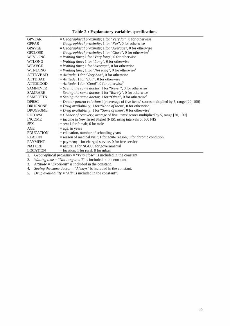
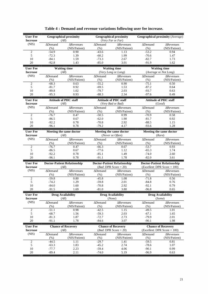
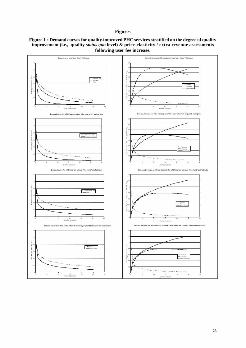
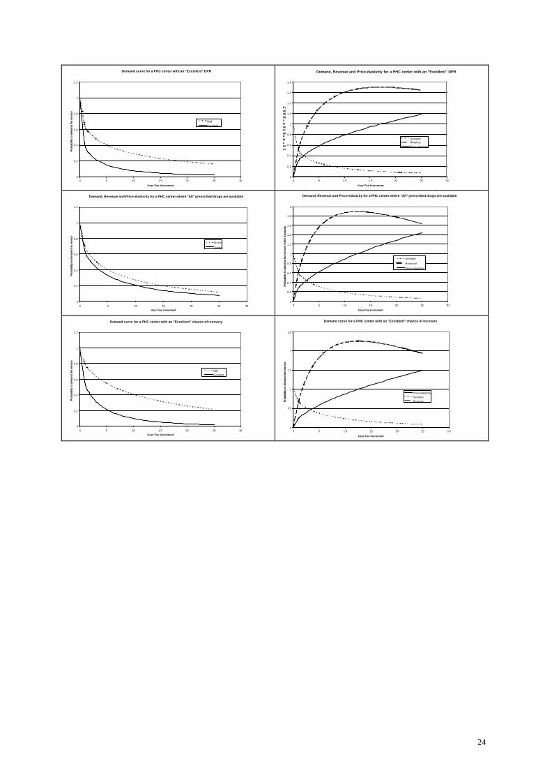
The model was first estimated using quality variables’ specifications presented in Table 2. Following, a series of Likelihood Ratio (LR) tests were conducted to assess equality amongst quality binary variables’ coefficients11, 12. Final regression results are listed in Table 3. In order to be able to interpret the resulting regression coefficients, one should notice that a smaller coefficient signifies a lower risk of not demanding the quality-improved service due to price increase. This can be quantified by taking the exponential of the regression coefficients which gives an estimation of the relative risk between the category of the independent variable of interest and the rest of the sample. Such interpretation would be useful for two-category qualitative variables (e.g., sex) and for quantitative variables (e.g., income). However, in order to be more illustrative about the role played by the amplitude of quality improvement - which is proposed to the respondent as an exchange of increasing user fees - on demand, the demand curve for the quality-improved health care was stratified over the different categories of quality status quo level. A lower quality status quo level indicates that a higher magnitude of quality improvement is being proposed to the individual in exchange of the price increase. Results for the seven quality attributes are presented in Figure 1. On the other hand, Weibull regression results are used to assess demand price-elasticity and PHC center's extra revenues following user fee increments; these are also presented in Figure 1. In both cases, demand, price-elasticity and revenues were estimated at the mean of all explanatory variables - other than UFI and “quality status quo level” 13. Consider the first line in the above list of graphs with different curves concerning a “Very Close” PHC center; i.e., a center with a “Geographical proximity” attribute being ameliorated to maximum. As mentioned above, this would imply different magnitudes of quality improvements to different individuals. Those who are living at an “Average” distance from the existing center would benefit from a lower magnitude of quality-improvement than those living “Very Far” from a center. Hence, the former shall be more penalized than the latter by an equal increase in user fees - as an exchange of having a “Very Close” PHC center. Sketching the demand curve for a “Very Close” PHC center, stratified over individual perception of the status quo level of “Geographical proximity” attribute, shows that demand curve declines more sharply when price increase is accompanied by lower magnitudes of quality improvements (i.e., with higher status quo levels). On the right hand-side the demand curve was sketched for the whole sample; i.e., all the sample undergoes the same price-increase to have a “Very Close” PHC center. We also presented on the same graphic how price elasticity and centers revenues vary with price-increase. The center can expect the highest extra revenues per user (1.59 NIS) when price-elasticity equals one. This shall occur at a user fee increment of 10.92 NIS. However, this would reduce demand by 85.4%. Similar analysis can be conducted for the different quality attributes in the study; and for categories of users benefiting from different magnitudes of quality improvements. In Table 4 we present some key figures of how “Demand” and PHC center's “Revenues” vary following user fee increase; results are first presented for the whole sample (i.e., quality improvement and user fee increase concern all the individuals in the sample), before being stratified over specified sample categories (e.g., improving the geographical proximity attribute only for the patients living “Very Far” or “Far” from the PHC center). Results suggest that respondents’ income has a significant effect on the way they would react vis-à-vis price variations. The risk that the patient ceases to demand the service following a user fee increment reduces as the patient’s income increases. This negative association between individual’s income and

11 For each quality attribute, respondents who belong to two consecutive categories of the quality variable; e.g., “Very Far” and “Far”, are regrouped and the new restrained model is estimated. The LR statistic is calculated as a difference between the log-likelihood of the complete and restrained models (ê and ?, respectively), as follows: LR = -2*(? - ê) ~ χ²(1). 12 The model was also estimated by adding income square to the explanatory variables; however, this have reduced the model predictive capacity. 13 Quality status quo level variable was introduced using sets of binary variables; thus, when comparisons are done, the binary variable representing the category of interest was substituted “One” and all the other binary variables were substituted “Zero”.

9

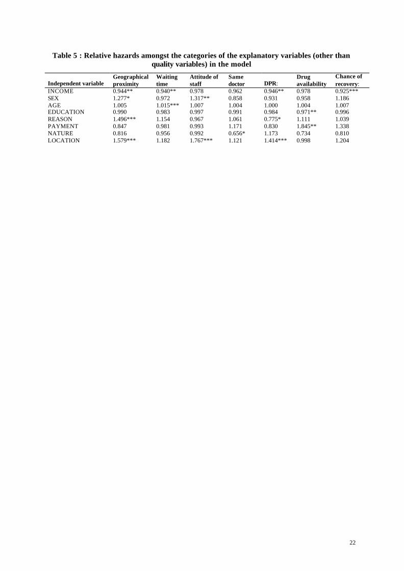
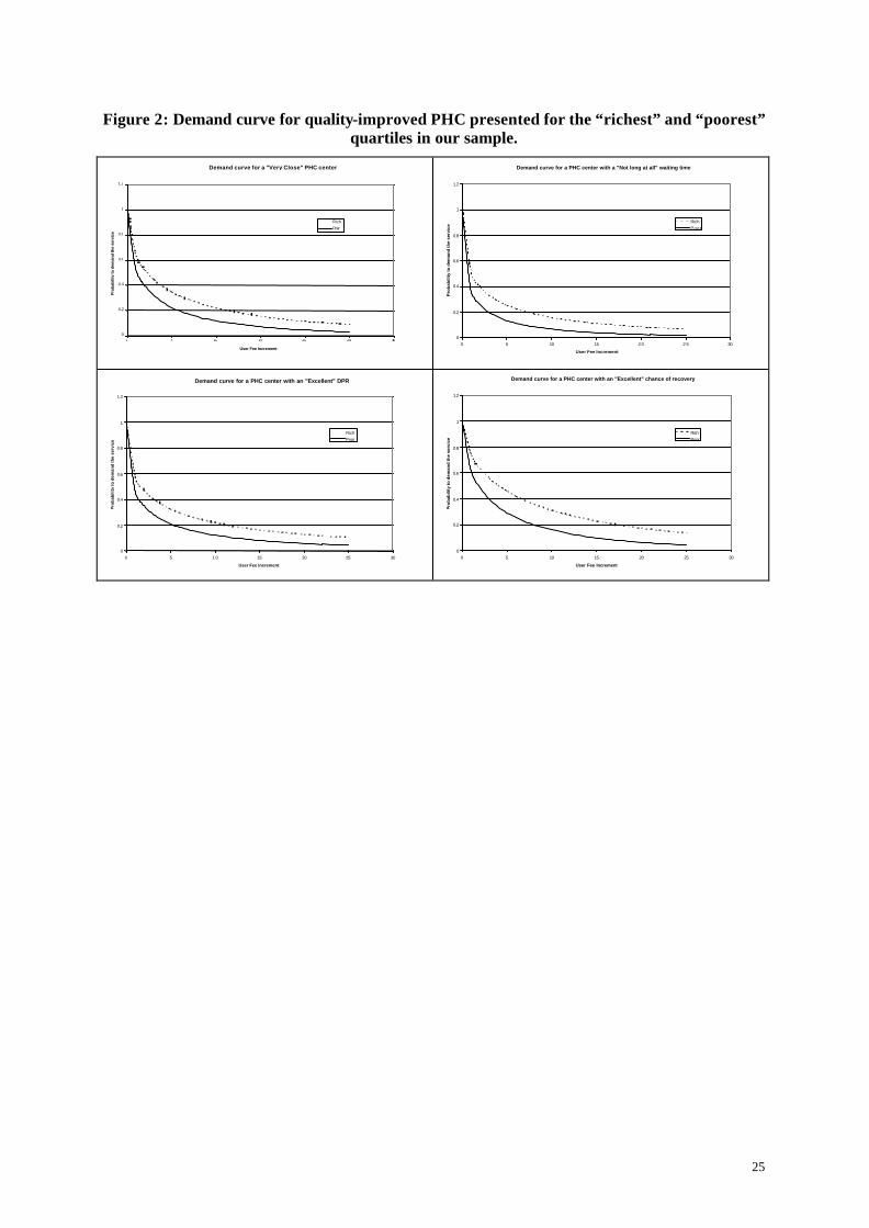
the risk of not demanding the service due to price increase was significant at 5 and 1% levels for four quality attributes; namely, geographical proximity, waiting time, doctor-patient relationship and chance of recovery. This can be interpreted as a positive income-elasticity, implying that health care is a “normal” good. The demand curve following improvements over each of the above four significant quality attributes were sketched in Figure 2 for the highest and the lowest income quartiles. The effect of the other explanatory variables in the model on demand was assessed by calculating the relative hazard as the exponential of the regression coefficients; results are presented in Table 5. A price increase accompanied by a quality improvement shall have a similar effect on the demand of male and female patients. Gender effect on demand was not significant excepted, when quality improvement concerns the geographical proximity and the attitude of the PHC center’s staff attributes. Here, the demand of women appears to be more negatively affected by the price increase than the corresponding demand of men, everything else being equal. On the other hand, the age of the patient seems not to influence her/his demand following the price-increase, except if the attribute to be ameliorated in combination with the price increase is waiting time. In this case, elder patients would be more negatively affected by the price increment. The demand of the more educated patients seems to be less affected by the price increments; however, the results were only significant for the drug availability attribute. Considering the reason for the medical visit whether it was for a chronic or an acute reason, the results were mixed. On one hand, the demand of chronic patients would be less affected (p < 0.01) following a user fee increase if the distance to the center was reduced to minimum. On the other hand, improving the doctor-patient relationship (including, time spent with the doctor to explain the health problem and the prescribed treatments) associated with a user fee increase shall decline the demand of chronic patients more than that of acute patients (p < 0.10). A user fee increase shall have a similar effect on the demand of patients who are used to be “charged” for the service and those who receive the service “free of charge”. An exception concerns the drug availability attribute. Here, the former seems not willing to pay more than what they are already paying to have all their prescribed treatments available in the center; thus, a user fee increment intended to finance such quality improvement shall affect more this group of patients. Furthermore, a price increase seems to have a similar effect whether it was experienced by a governmental or a NGO PHC center; however, the NGO clientele would be less affected by the price increase if the latter was intended to assure that the patients be able to meet the same doctor every time she/he comes to the center. Finally, price-increase shall have a more negative effect on demand if they were implemented in rural PHC centers than if they were exercised by urban PHC centers. This effect appears to be highly significant if the mobilized revenues were used to improve one of the following attributes: geographical proximity , attitude of the staff or doctor-patient relationship .

5. Discussion: The above analysis demonstrates how do demand, price-elasticity and center's revenues vary with user fee-increase, when the latter is accompanied with improvements in the quality of provided health care. Results suggest that the negative effect of user fee-increase on demand can be compensated, at least in part, by improving the quality of the service. On the other hand, the more important the quality improvement is, the less negative effect the user fee shall have on demand. This shall support previous study results on the positive compensatory effect of quality improvement on demand (Abel-Smith and Rawal 1992; Weaver, Ndamobissi et al. 1996). On the other hand, our model allows to estimate a price-elasticity that varies with the user fee level; which remains more consistent with the economic theory than the restrictive assumption of constant price-elasticity. The latter can be found in most of the studies which have used simple descriptive techniques or econometric modeling to assess price-demand elasticity (Gertler and Hammer 1997; Cissé, Luchini et al. 2002). The analogy presented in our paper between the demand function and survival (duration) analysis has been pointed to by Johannesson and Jonsson (Johannesson and Jonsson 1991). In their paper, the

10

authors discuss the estimation of mean and median WTP values obtained using dichotomous choice (DC) elicitation technique14. Given the binary nature of DC CV studies (yes/no), discrete regression models, such as, logistic function specification can be used to directly assess the probability of accepting a bid as a function of a set of explanatory variables (including, the bid itself). Thus, the demand function is directly obtained, as well as, the marginal effects of price and income on demand, using logit or probit estimation techniques. The authors note that: “The function that is calculated (i.e., the probability to accept a bid) can be viewed as a survival function with respect to willingness to pay (bid)”; they also allude to the similarities between the computation of willingness to pay using discrete data and the computation of life expectancy15. In our study, the use of duration modeling methodology allows us, using continuous WTP values, to get an indirect estimate of the probability to demand the quality-improved service as a function of service’s price and adjusting for individual’s socio-demographic and economic characteristics. The Weibull distribution appears to be adapted to our study analysis context. It resulted by estimations consistent with our a priori expectations; especially, concerning the positive effect of the amplitude of quality improvements and respondents’ income on the probability to demand the quality-improved service. Moreover, the effect of the set of explanatory variables included in the model, as it is suggested by the Weibull regression analysis, are highly comparable to results obtained using Tobit regression used to analyze the determinants of stated WTP values (published elsewhere, see Mataria et al. (Mataria, Donaldson et al. 2002)). Our results can be added to previous evidence on the applicability of CV in developing countries, and on its acceptability by the respondents over there (Whittington 1998). Moreover, the validity proofs presented by our analysis coincide with previous results on the validity of CV in assessing health care in developing countries (Hassan, El Nahal et al. 1994; Asenso-Okyere, Osei-Akoto et al. 1997; Onwujekwe, Chima et al. 2002). In an attempt to assess the validity and reliability of CV in eliciting the value of non-marketed amenities, the NOAA panel16 advanced a list of recommendations to be respected by forthcoming CV studies to ensure results’ validity and reliability (Portney 1994). Excepted for the elicitation technique - recommended to be the DC format (Arrow, Solow et al. 1993) - our study conformed to all other recommendations (see Mataria et al. (Mataria, Donaldson et al. 2002)). The panel preference for the DC elicitation technique is based on the assumption that DC elicitation format yields incentive-compatible results; i.e., respondents shall answer such hypothetical questions as if they were involved in real economic commitments because, they have no incentives to misrepresent. However, the question remains controversial for researchers who were able to get valid results using other elicitation techniques (Donaldson, Thomas et al. 1997); and for others who detected significant statistical differences between respondents’ answers to hypothetical and real DC CV randomized and controlled experiments (Cummings, Harrison et al. 1995)17. Hence, some authors find that the arguments raised in favor of the DC format unpersuasive mainly that, open-ended questions are able to result in “valid” WTP estimates and much more information (Gyldmark and Morrison 2001). Policy implications: Government can intervene in the health care sector to pursue different public objectives, extending from: correcting health care market failures that causes health outcomes to be lower than what they

14 Using the dichotomous choice technique (also known as closed-ended or referendum format) consists of asking the respondent whether or not she/he would be willing to pay a certain amount of money for the good in question; researchers usually vary the proposed amount from one individual to another to be able to estimate a demand function. 15 For an illustrative example of how to calculate price-elasticity following DC WTP data, see: [Population Council (1998). “Price elasticity of demand for reproductive health services at an Ecuadorian private voluntary organization.” at: http://www.popcouncil.org/pdfs/inopal/015.pdf ] (accessed in December, 19th 2002). 16 This is a panel of economic experts chaired by Nobel-price laureates, Kenneth Arrow and Robert Solow, convened in 1992 by the U.S. Department of Commerce – acting through the National Oceanic and Atmospheric Administration (NOAA) - to assess the reliability of CV to conduct natural resource damage assessments. 17 Under their study experimental design, Cummings and Harrison (1995) define real DC CV studies as those where payment and provision of the good actually take place. They argue that under this condition the respondent shall perceive his expected utility being affected by the possibility of the good actually being provided and thus has no incentive to misrepresent. They go on to say that such a presumption cannot be made regarding the hypothetical DC method.

11

otherwise could be, to, subsidizing poor’s access to medical care. Providing “free” health care services can assure - yet, to some extent - an equitable utilization of health care services by different population income-classes. However, given scarce health care resources, and in order to avoid inefficient utilization of provided services, users (or potential users) are required to participate in the financing mechanism. This can be done in a direct manner through payments at the point of consumption, or indirectly through tax payments and insurance premiums. Using ex ante indirect financing mechanisms would permit, in a much simpler way, to adjust for the second dimension of governmental objectives in the health sector; i.e., equity in access. Indeed, such financing mechanisms allow - under well established and controlled public financial system - to adjust individuals’ financial contributions on one’s ability to pay. Due to this reason - and others including uncertainty features of health care demand and individuals’ risk aversion characteristics (Arrow 1963) - most developed countries adopted the latter as their major form of finance for the health sector. It would be difficult for developing countries under current local economic environment (i.e., insufficient public resources, widespread poverty conditions, insufficiently developed tax systems, etc.) to advocate such ex ante financing mechanisms. Hence, direct-payment policies through user fees at the point of consumption were recommended (World-Bank 1987). In order to control for the equity dimension - mainly that research results (including ours) indicate different effects of price-increase on the demand of individuals coming from different income classes - efforts should be invested in classifying the population on a valid well-being measurement scale, and in identifying those disposing the lowest wealth. This shall serve as a preliminary step in structuring a pricing system that respects different individuals’ financial capacities. Assessing respondents’ WTP values for health care services and identifying its determinants represents another solution to the question of price structuring. Indeed, the latter takes into consideration not only wealth measurements but also individuals’ preferences and own choices with regard to health care (Donaldson 1999); which remains more consistent with welfare economic principles (O'Brien and Drummond 1994). A policymaker may be more interested in the distribution of benefits (gained or lost) from a policy change than she/he is in the actual aggregate comparison of costs and benefits - summarized by the program net social benefits (NSB). This is specially true for programs revealed to be potentially Pareto-improving. Some authors (Mitchell and Carson 1989; Foreit and Foreit 2003) propose to plot separate WTP distribution curves (decumulative distribution function) for different sub-samples stratified on some characteristics of interest; e.g., gender, age, education or income. The introduction of individual socio-demographic and economic characteristics directly in the demand function shall enable health policymakers to assess directly the distributional effects of the health program under investigation. In summary, disposing information about individuals’ WTP values permits to identify those public interventions in the health sector that are worthwhile for the population; and to assess the extent to which private resources could be mobilized to assist in financing the intervention in question. Consequently, this shall enlighten public decisions of where and whom to subsidize; and thus be used as a basis to elaborate price-discrimination policies. Study limitations: Beside the major limitation of any contingent valuation study which consists of its dependence on hypothetical scenarios to predict patients reaction, our study presents some other limitations. Demand analysis was restricted to a random sample picked up among the current users of the investigated services. However, investments in the quality of the provided services would probably attract new users who were seeking health care in other health sectors, eventually, private clinics. This shall not raise a problem if we are only interested in the demand of the current clientele, which might - most probably - not be the case. Therefore, our estimation of demand elasticity and extra revenues should be taken as conservative. One of the implicit assumptions in our model is the inter-attribute independence; i.e., the value of improvements over one attribute does not depend on the level of other attributes. However, a patient

12

might value improvements over one attribute more or less depending upon how well the service is placed on other attributes’ measurement scales; e.g., a patient might support having a “Very far” PHC center – and thus value less improvements over the “geographical proximity” attribute – if she/he knows that she/he shall not wait long before meeting the doctor. Further analysis is needed to verify the existence of such inter-attribute dependence and to adjust for it. A practical limitation that might have affected our study results is, unfortunately, the bad political situation at the time of fieldwork. Check points were installed at all cities’ entries depriving rural population from an easy circulation to and out of the cities and between villages. This had strongly affected travel time to health centers. The study period was also characterized with a high unemployment rate which would have affected respondents’ incomes and their appreciation of “Time”; some respondents said that they were willing to wait and not to pay because they have nothing else to do, except being home. Given that this situation had persisted for a long time before the beginning of the study, it can be considered that this had become the “normal” living situation. Finally, it would be interesting to compare our results from the Weibull parametric modeling with those from less restrictive non-parametric survival models; e.g., piece-wise models. These can also be used to analyze continuous WTP data based on our conceptual framework, and without being restricted to an underlying functional form. This was left for further investigations.

6. Conclusion: Demand and price-elasticity of quality-improved PHC were assessed using patients’ WTP values for ameliorating health care quality level. Conceptual analysis of respondents’ reaction to stated monetary valuation questions was used to model the demand function using a parametric duration model. Results are consistent with economic theory and with our a priori expectations. It is argued that, WTP data hold much more information relevant to demand modeling than simple descriptive analysis used in previous literature. Validating our approach shall promote another potential application for the CV beside cost-benefit analysis. Information about users’ WTP values allow to justify (or not) the implementation of different quality improvements; and furthermore, to help in elaborating optimal and successful pricing policies for PHC services. The latter shall integrate different income, social and demographic classes’ own preferences and financial capacities in the decision-making process; thus, help to adjust public efficiency objectives on equity dimensions. Operational decision tools elaborated in developed countries shall not be automatically and “blindly” transposed to developing countries without conceptual and empirical adaptations. However, developing countries, usually deprived from social security schemes, where patients pay for medical services, represent a more fertile field for CV with much less hypothetical bias and higher method’s validity. We conclude that WTP approach is a potentially valuable tool with applications going beyond economic evaluation; however, our study remains an exploratory one and the empirical agenda will be large before recognizing the CV as a valid and reliable measurement tool.

13

Appendix Appendix A:

Quality attributes and their corresponding measurement scales.

Attribute Measurement Scale 1. Geographical proximity Very far, Far, Average, Close, Very close. 2. Waiting time Very long, Long, Average, Not long, Not long at all. 3. Attitude of PHC center's staff toward the respondent Excellent, Good, Bad, Very bad. 4. Being able to see the same doctor at every visit Always, Often, Rarely, Never. 5. Being able to discuss her/his problem with the doctor

and receive sufficient information about her/his health state and the prescribed treatment(s)

Multi-item Likert scaling; range: [20,100] (continuous). Items: 1. I stayed sufficient time with the doctor. 2. The doctor explained to me my health problem. 3. The doctor explained to me how to use the prescribed treatment(s). 4. The doctor explained to me what I should do to prevent (or not to complicate) my health problem in the future. 5. The information was clear and sufficient.

6. Being able to purchase the prescribed treatment(s) at the center

All, Some of them, None.

7. Chance of recovery Multi-item Likert scaling; range:[20,100] (continuous). Items: 1. I usually get recovered after being examined by the doctor of the center. 2. Many times, I need to go to a private clinic to be re-examined by a better doctor. 3. The doctor who examined me was a good doctor who knows what he is doing. 4. Private doctors are more competent. 5. In general, I prefer to go to private clinic.

14

Appendix B: The seven partial valuation questions and the semi-holistic valuation question:

• benefit from a PHC center similar to this one and located “Very close” to your home?

• have a PHC center “Very close” to your home;

• have a PHC center with a “waiting time” that you estimate as “Not long at all”?

• have a PHC center with a “Waiting time” that you estimate as “Not long at all”;

• benefit from an “Excellent” attitude from the PHC center staff?

• benefit from an “Excellent” attitude from the PHC center staff;

• be able to see the same health professional every time you come to the center?

• “Yes”à • be able to see the same health professional every time you come to the center;

• be able to stay sufficient time with the doctor to discuss with him your health problem, receive sufficient and clear information about your disease and the prescribed treatment(s)?

• be able to stay sufficient time with the doctor to discuss with him your health problem, receive sufficient and clear information about your disease and the prescribed treatment(s);

• be able to find the prescribed treatment(s) “always” available in the center?

• What is the maximum amount of money that you would be willing to pay, extra to what you currently pay, in order to …

• be able to find the prescribed treatment(s) “always” available in the center;

Would you be willing to pay any amount of money (even small amounts like 1, 2, 3 or 4 NIS) more than what you already pay in order to …

• be examined by more competent doctors and to have a higher chance of recovery?

• be examined by more competent doctors and to have a higher chance of recovery;

• knowing

that this extra amount of money will be paid at every visit?à

Payment Card

• “No” à • Why? ______________________________________________________

15

Appendix C: Demand curve by geographical proximity perception

Pro

babi

lity

to d

eman

d th

e se

rvic

e

User Fee Increment0 10 20 30

0.00

0.25

0.50

0.75

1.00

________Very Far__ _ __ _ Far_ _ _ _ _ Close………… Very close

Log-rank test:Probability > χ² = < 0.00005

Demand curve by income

Pro

babi

lity

to d

eman

d th

e se

rvic

e

Use Fee Increment0 10 20 30

0.00

0.25

0.50

0.75

1.00

______ Poor__ __ _ Rich

Log-rank test:Probability> χ² = 0.0036

Demand curve by sex

Pro

babi

lity

to d

eman

d th

e se

rvic

e

User Fee Increment0 10 20 30

0.00

0.25

0.50

0.75

1.00

______ Male_ __ __ Female

Log-rank test:Probability > χ² < 0.00005

Demand curve by age

Pro

babi

lity

to d

eman

d th

e se

rvic

e

User Fee Increment0 10 20 30

0.00

0.25

0.50

0.75

1.00

______ Young_ __ __ Old

Long-rank test:Probability > χ² = 0.3132

Demand curve by education

Pro

babi

lity

to d

eman

d th

e se

rvic

e

User Fee Increment0 10 20 30

0.00

0.25

0.50

0.75

1.00

_____ Low __ __ High

Log-rank test:Probability > χ² = 0.0118

Demand curve by reason

Pro

babi

lity

to d

eman

d th

e se

rvic

e

User Fee Increment0 10 20 30

0.00

0.25

0.50

0.75

1.00

______ Chronic_ __ __ Acute

Log-rank test:Probability > χ² = 0.0586

Demand curve by payment

Pro

babi

lity

to d

eman

d th

e se

rvic

e

User Fee Increment0 10 20 30

0.00

0.25

0.50

0.75

1.00

______ Free_ __ __ Charged

Log-rank test:Probability > χ² = 0.0066

Demand curve by nature

Pro

babi

lity

to d

eman

d th

e se

rvic

e

User Fee Increment0 10 20 30

0.00

0.25

0.50

0.75

1.00

_____ Government_ __ _ NGO

Log-rank test:Probability > χ² = 0.0058

Demand curve by location

Pro

babi

lity

to d

eman

d th

e se

rvic

e

User Fee Increment0 10 20 30

0.00

0.25

0.50

0.75

1.00

______ Urban_ __ __ Rural

Log-rank test:Probability > χ² = < 0.00005

16

References

Abel-Smith, B. and P. Rawal (1992). "Can the poor afford free health service. A case study of Tanzania." Health Policy and Planning 7(4): 329-341.

Akaike, H. (1981). "Likelihood of a Model and Information Criteria." Journal of Econometrics 16(1): 3-14. Alderman, H. and V. Lavy (1996). "Household responses to public health services: cost and quality tradeoffs."

The World Bank Research Observer 11(1): 3-22. Arrow, K. (1963). "Uncertainty and the welfare economics of medical care." American Economic Review 53(5):

941-973. Arrow, K., R. Solow, et al. (1993). "Report of the NOAA Panel of Contingent Valuation." Federal Register

58(10): 4601-4614. Asenso-Okyere, W. K., I. Osei-Akoto, et al. (1997). "Willingness to pay for health insurance in a developing

economy. A pilot study of the informal sector of Ghana using contingent valuation." Health Policy 42(3): 223-37.

Bratt, J. H., M. A. Weaver, et al. (2002). "The impact of price changes on demand for family planning and reproductive health services in Ecuador." Health Policy and Planning 17(3): 281-7.

Cissé, B., S. Luchini, et al. (2002). "Les effets des politiques de recouvrement des coûts sur la demande de soins dans les Pays En Développement: les raisons de résultats contradictoire." Revue Française d'Economie Submitted.

Cummings, R. G., G. W. Harrison, et al. (1995). "Homegrown values and hypothetical surveys: is the dichotomous choice approach incentive-compatible?" The American Economic Review 85(1): 260-266.

Donaldson, C. (1999). "Valuing the benefits of publicly-provided health care: does 'ability to pay' preclude the use of 'willingness to pay'?" Social Science & Medicine 49(4): 551-63.

Donaldson, C., R. Thomas, et al. (1997). "Validity of open-ended and payment scale approaches to eliciting willingness to pay." Applied Economics 29: 79-84.

Dumoulin, J. (1993). "Le paiement des soins par les usagers dans les pays d'afrique sub-saharienne : rationalité économique et autres questions subséquentes." Sciences Sociales et Santé 11(2): 81-119.

Foreit, J. R. and K. G. F. Foreit (2003). "The reliability and validity of willingness to pay surveys for reproductive health pricing decisions in developing countries." Health Policy 63(1): 37-47.

Gertler, P. and J. Molyneaux (1997). Experimental evidence on the effect of raising user fees for publicly delivered health care services: utilization, health outcomes, and private provider response. Santa Monica, CA.

Gertler, P. J. and J. S. Hammer (1997). Strategies for pricing publicly provided health services, University of California at Berkeley and The World Bank: 37.

Greene, W. (2000). Econometric Analysis . New Jersey, Prentice-Hall, Inc. Gyldmark, M. and G. C. Morrison (2001). "Demand for health care in Denmark: results of a national sample

survey using contingent valuation." Social Science & Medicine 53(8): 1023-36. Hassan, E., N. El Nahal, et al. (1994). "Acceptability of the once-a-month injectable contraceptives cyclofem and

mesigyna in Egypt." Contraception 49: 469-488. Johannesson, M. and B. Jonsson (1991). "Economic evaluation in health care: is there a role for cost-benefit

analysis?" Health Policy 17(1): 1-23. Kennedy, P. (1998). A guide to Econometrics. Massachusetts, The MIT Press. Klose, T. (1999). "The contingent valuation method in health care." Health Policy 47(2): 97-123. Mataria, A., C. Donaldson, et al. (2002). "Patients' Willingness to Pay for Improving the Quality of Primary

Health Care Services in Palestine: What's about the validity of contingent valuation?" Journal of Health Economics Submitted.

McPake, B., K. Hanson, et al. (1993). "Community finance of health care in Africa: An evaluation of the Bamako Initiative." Social Science & Medicine 36(11): 1383-1395.

Mitchell, R. and R. Carson (1989). Using Surveys to Value Public Goods: The Contingent Valuation Method. Washington DC, Resources for the Futhure.

Mwabu, G., M. Ainsworth, et al. (1993). "Quality of medical care and choice of medical treatment in Kenya." Journal of Human Resources 28(4): 838-862.

Newhouse, J. (1995). Free for all, Cambridge: Harvard University Press. O'Brien, B. and A. Gafni (1996). "When do the "dollars" make sense? Toward a conceptual framework for

contingent valuation studies in health care." Medical Decision Making 16(3): 288-99. O'Brien, B. J. and M. F. Drummond (1994). "Statistical versus quantitative significance in the socioeconomic

evaluation of medicines." Pharmacoeconomics 5(5): 389-98. Onwujekwe, O., R. Chima, et al. (2002). "Altruistic willingness to pay in community-based sales of insecticide-

treated nets exists in Nigeria." Social Science & Medicine 54(4): 519-27.

17

Onwujekwe, O., R. Chima, et al. (2001). "Hypothetical and actual willingness to pay for insecticide-treated nets in five Nigerian communities." Tropical Medicine & International Health 6(7): 545-53.

Portney, P. R. (1994). "The contingent valuation debate: Why economists should care." Journal of Economic Perspectives 8(4): 3-17.

StataCorp (2001). Stata Statistical Software: Release 7.0. College Station, TX, Stata Corporation. Varian, H. (2000). Introduction à la microéconomie. Paris, Boeck Université. Waddington, C. J. and K. A. Enyimayew (1990). "A price to pay: the impact of user charges in the Volta region

of Ghana." International Journal of Health Planning and Management 5(4): 287-312. Weaver, M., R. Ndamobissi, et al. (1996). "Willingness to pay for child survival: results of a national survey in

Central African Republic." Social Science & Medicine 43(6): 985-98. Whittington, D. (1998). "Administering contingent valuation surveys in developing countries." World

development 26(1): 21-30. Whittington, D., O. Matsui-Santana, et al. (2002). "Private demand for a HIV/AIDS vaccine: evidence from

Guadalajara, Mexico." Vaccine 20: 2585-2591. World-Bank (1987). Financing Health Services in Development Countries: An Agenda for Reform. Washington,

World Bank: 99.

18

Tables

Table 1 : Sample characteristics

Characteristic Mean (±S.D.*) / percentage %Female 76.8% Age 35.9 (± 13.7) % Living in a village1 84.2% % Married2 82.2% Person/household 7.4 (± 3.6) Person<14 years 3.1 (± 2.2) Person in charge 7.5 (± 3.7) No. of schooling years 8.5 (± 4.6) % Housewife3 63.8% % Insured 75.4% % Suffer from an acute condition4 65.5% % Examined by generalists5 67.5% % Came more than once during last year 89.2% % Received the service “free of charge”6 54.5% Household monthly Income 1830.3 (± 1215.6) NIS

* S.D. = standard deviation. 1. 12.2% live in a city and 3.6% live in a refugee-camp. 2. 11.7% single, 4.7% widowed and 1.2% divorced. 3. 11.2% employed, 7.5% workers, 6.9% independent, 4.7% unemployed, 4.1% students and 1.4% others. 4. 21.8% chronic problems, 4.2% pregnancy consultation, 2.4% emergency, 6% other reasons. 5. 32.5% (n=161) examined by specialists, mainly recruited by NGO-PHC centers (n=150). 6. Global mean user fees = 6.3 (±8.1) NIS.

19

Table 2 : Explanatory variables specification.

GPVFAR = Geographical proximity; 1 for “Very far”, 0 for otherwise GPFAR = Geographical proximity; 1 for “Far”, 0 for otherwise GPAVGE = Geographical proximity; 1 for “Average”, 0 for otherwise GPCLOSE = Geographical proximity; 1 for “Close”, 0 for otherwise1 WTVLONG = Waiting time ; 1 for “Very long”, 0 for otherwise WTLONG = Waiting time ; 1 for “Long”, 0 for otherwise WTAVGE = Waiting time ; 1 for “Average”, 0 for otherwise WTNLONG = Waiting time ; 1 for “Not long”, 0 for otherwise2 ATTDVBAD = Attitude; 1 for “Very bad”, 0 for otherwise ATTDBAD = Attitude; 1 for “Bad”, 0 for otherwise ATTDGOOD = Attitude; 1 for “Good”, 0 for otherwise3 SAMNEVER = Seeing the same doctor; 1 for “Never”, 0 for otherwise SAMRARE = Seeing the same doctor; 1 for “Rarely”, 0 for otherwise SAMEOFTN = Seeing the same doctor; 1 for “Often”, 0 for otherwise4 DPRSC = Doctor-patient relationship; average of five items’ scores multiplied by 5, range [20, 100] DRUGNONE = Drug availability; 1 for “None of them”, 0 for otherwise DRUGSOME = Drug availability; 1 for “Some of them”, 0 for otherwise5 RECOVSC = Chance of recovery; average of five items’ scores multiplied by 5, range [20, 100] INCOME = income in New Israel Shekel (NIS), using intervals of 500 NIS SEX = sex; 1 for female, 0 for male AGE = age, in years EDUCATION = education, number of schooling years REASON = reason of medical visit; 1 for acute reason, 0 for chronic condition PAYMENT = payment; 1 for charged service, 0 for free service NATURE = nature; 1 for NGO, 0 for governmental LOCATION = location; 1 for rural, 0 for urban 1. Geographical proximity = “Very close” is included in the constant. 2. Waiting time = “Not long at all” is included in the constant. 3. Attitude = “Excellent” is included in the constant. 4. Seeing the same doctor = “Always” is included in the constant. 5. Drug availability = “All” is included in the constant”.

20

Table 3 : Weibull regression results

Independent variable Geographical Proximity

Waiting time

Attitude of staff

Same doctor DPR♣

Drug availability

Chance of recovery♣

B (B SE) B (B SE) B (B SE) B (B SE) B (B SE) B (B SE) B (B SE) Constant 1.833***

(0.547) -0.121 (0.411)

-0.160 (0.395)

0.641 (0.419)

-0.462 (0.381)

-0.653* (0.391)

-1.815*** (0.443)

GPVFAR_FAR -3.048*** (0.346)

- - - - - -

GPAVGE -2.765*** (0.350)

- - - - - -

GPCLOSE -2.031*** (0.361)

- - - - - -

WTVLONG_LONG - -0.636*** (0.153)

- - - - -

WTAVGE_NLONG - -0.088 (0.148)

- - - - -

ATTDVBAD_BAD - - -0.899*** (0.249)

- - - -

ATTDGOOD - - -0.338*** (0.116)

- - - -

SAMNEVER_OFTEN - - - -0.535*** (0.152)

- - -

SAMRARE - - - -0.880*** (0.188)

- - -

DPRSC - - - - 0.009*** (0.003)

- -

DRUGNONE - - - - - -0.293 (0.205)

-

DRUGSOME - - - - - -0.082 (0.150)

-

RECOVSC - - - - - - 0.012*** (0.003)

INCOME -0.058** (0.026)

-0.062** (0.025)

-0.022 (0.023)

-0.039 (0.025)

-0.056** (0.024)

-0.022 (0.024)

-0.078*** (0.024)

SEX 0.244* (0.138)

-0.028 (0.131)

0.275** (0.136)

-0.154 (0.152)

-0.072 (0.140)

-0.042 (0.137)

0.171 (0.137)

AGE 0.005 (0.006)

0.015*** (0.005)

0.007 (0.005)

0.004 (0.005)

0.0004 (0.005)

0.004 (0.005)

0.007 (0.005)

EDUCATION -0.010 (0.015)

-0.017 (0.014)

-0.003 (0.015)

-0.009 (0.016)

-0.017 (0.015)

-0.030** (0.015)

-0.004 (0.015)

REASON 0.402*** (0.150)

0.143 (0.143)

-0.033 (0.148)

0.059 (0.146)

-0.255* (0.140)

0.105 (0.145)

0.039 (0.143)

PAYMENT -0.166 (0.232)

-0.020 (0.260)

-0.007 (0.249)

0.158 (0.234)

-0.186 (0.249)

0.613** (0.287)

0.291 (0.249)

NATURE -0.204 (0.234)

-0.045 (0.262)

-0.008 (0.252)

-0.422* (0.246)

0.159 (0.258)

-0.309 (0.286)

-0.210 (0.254)

LOCATION 0.457*** (0.121)

0.168 (0.115)

0.569*** (0.121)

0.114 (0.145)

0.347*** (0.124)

-0.002 (0.123)

0.185 (0.122)

Alpha 0.520*** (0.021)

0.427*** (0.017)

0.348*** (0.013)

0.348*** (0.014)

0.433*** (0.018)

0.529*** (0.023)

0.582*** (0.043)

No. of observations 400 401 401 348 400 375 399 Log likelihood -899.30 -975.31 -1037.60 -899.88 -973.60 -850.74 -874.75 Probability > χ² <0.00005 <0.00005 <0.00005 <0.00005 <0.00005 0.0046 <0.00005 Notes: B = coefficient, SE B = standard error of the coefficient. * = P < 0.10; ** = P < 0.05; *** = P < 0.01. ♣: DPR score and Chance of Recovery score; range [20 , 100].

21

Table 4 : Demand and revenue variations following user fee increase.

Geographical proximity (All)

Geographical proximity (Very Far or Far)

Geographical proximity (Average) User Fee Increase

(NIS) ∆Demand (%)

∆Revenues (NIS/Patient)

∆Demand (%)

∆Revenues (NIS/Patient)

∆Demand (%)

∆Revenues (NIS/Patient)

2 -54.9 0.90 -43.6 1.13 -53.2 0.94 5 -72.3 1.39 -60.2 1.99 -70.6 1.47 10 -84.1 1.59 -73.3 2.67 -82.7 1.73 20 -92.8 1.43 -85.0 3.01 -91.9 1.62

Waiting time (All)

Waiting time (Very Long or Long)

Waiting time (Average or Not Long)

User Fee Increase

(NIS) ∆Demand (%)

∆Revenues (NIS/Patient)

∆Demand (%)

∆Revenues (NIS/Patient)

∆Demand (%)

∆Revenues (NIS/Patient)

2 -68.3 0.63 -55.2 0.90 -75.1 0.50 5 -81.7 0.92 -69.5 1.53 -87.2 0.64 10 -89.8 1.02 -79.7 2.03 -93.7 0.63 20 -95.3 0.93 -88.3 2.34 -97.6 0.49

Attitude of PHC staff (All)

Attitude of PHC staff (Very Bad or Bad)

Attitude of PHC staff (Good)

User Fee Increase

(NIS) ∆Demand (%)

∆Revenues (NIS/Patient)

∆Demand (%)

∆Revenues (NIS/Patient)

∆Demand (%)

∆Revenues (NIS/Patient)

2 -76.7 0.47 -50.5 0.99 -70.9 0.58 5 -86.5 0.67 -62.0 1.90 -81.7 0.92 10 -92.2 0.78 -70.8 2.92 -88.5 1.15 20 -96.1 0.78 -79.2 4.17 -93.6 1.28

Meeting the same doctor (All)

Meeting the same doctor (Never or Often)

Meeting the same doctor (Rare)

User Fee Increase

(NIS) ∆Demand (%)

∆Revenues (NIS/Patient)

∆Demand (%)

∆Revenues (NIS/Patient)

∆Demand (%)

∆Revenues (NIS/Patient)

2 -76.7 0.47 -66.3 0.67 -53.7 0.93 5 -86.5 0.67 -77.6 1.12 -65.3 1.74 10 -92.2 0.78 -85.1 1.49 -74.0 2.60 20 -96.1 0.78 -91.1 1.78 -82.0 3.61

Doctor-Patient Relationship (All)

Doctor-Patient Relationship (Bad: DPR Score = 20)

Doctor-Patient Relationship (Excellent: DPR Score = 100)

User Fee Increase

(NIS) ∆Demand (%)

∆Revenues (NIS/Patient)

∆Demand (%)

∆Revenues (NIS/Patient)

∆Demand (%)

∆Revenues (NIS/Patient)

2 -59.8 0.80 -45.8 1.08 -71.8 0.56 5 -74.2 1.29 -59.8 2.01 -84.8 0.76 10 -84.0 1.60 -70.8 2.92 -92.1 0.79 20 -91.5 1.69 -81.0 3.80 -96.8 0.65

Drug Availability (All)

Drug Availability (None)

Drug Availability (Some)

User Fee Increase

(NIS) ∆Demand (%)

∆Revenues (NIS/Patient)

∆Demand (%)

∆Revenues (NIS/Patient)

∆Demand (%)

∆Revenues (NIS/Patient)

2 -51.1 0.98 -42.5 1.15 -49.5 1.01 5 -68.7 1.56 -59.3 2.03 -67.1 1.65 10 -81.3 1.87 -72.7 2.73 -79.9 2.01 20 -91.1 1.78 -84.6 3.07 -90.1 1.98

Chance of Recovery (All)

Chance of Recovery (Bad: DPR Score = 20)

Chance of Recovery (Excellent: DPR Score = 100)

User Fee Increase

(NIS) ∆Demand (%)

∆Revenues (NIS/Patient)

∆Demand (%)

∆Revenues (NIS/Patient)

∆Demand (%)

∆Revenues (NIS/Patient)

2 -44.5 1.11 -29.7 1.41 -59.5 0.81 5 -63.3 1.83 -45.2 2.74 -78.6 1.07 10 -77.7 2.23 -59.4 4.06 -90.1 0.99 20 -89.4 2.11 -74.0 5.19 -96.9 0.63

22

Table 5 : Relative hazards amongst the categories of the explanatory variables (other than quality variables) in the model

Independent variable Geographical proximity

Waiting time

Attitude of staff

Same doctor DPR♣

Drug availability

Chance of recovery♣

INCOME 0.944** 0.940** 0.978 0.962 0.946** 0.978 0.925*** SEX 1.277* 0.972 1.317** 0.858 0.931 0.958 1.186 AGE 1.005 1.015*** 1.007 1.004 1.000 1.004 1.007 EDUCATION 0.990 0.983 0.997 0.991 0.984 0.971** 0.996 REASON 1.496*** 1.154 0.967 1.061 0.775* 1.111 1.039 PAYMENT 0.847 0.981 0.993 1.171 0.830 1.845** 1.338 NATURE 0.816 0.956 0.992 0.656* 1.173 0.734 0.810 LOCATION 1.579*** 1.182 1.767*** 1.121 1.414*** 0.998 1.204

23

Figures

Figure 1 : Demand curves for quality-improved PHC services stratified on the degree of quality improvement (i.e., quality status quo level) & price-elasticity / extra revenue assessments

following user fee increase. Demand curve for a "Very Close" PHC center

0

0.2

0.4

0.6

0.8

1

1.2

0 5 10 15 20 25 3 0User Fee Increment

Pro

babi

lity

to d

eman

d th

e se

rvic

e

Very Far - FarAverageClose

Demand, Revenue and Price-elasticity for a "Very Close" PHC center

0

0.2

0.4

0.6

0.8

1

1.2

1.4

1.6

1.8

0 5 10 15 20 2 5 30User Fee Increment

Pro

babi

lity

to d

eman

d th

e se

rvic

e / N

IS /

Ela

stic

ity

DemandRevenuePrice-elasticity

Demand curve for a PHC center with a "Not long at all" waiting time

0

0.2

0.4

0.6

0.8

1

1.2

0 5 10 15 20 25 30

User Fee Increment

Pro

babi

lity

to d

eman

d th

e se

rvic

e

Very Long - Long

Average - Not Long

Demand, Revenue and Price elasticity for a PHC center with a "Not long at all" waiting time

0

0.2

0.4

0.6

0.8

1

1.2

1.4

1.6

0 5 10 15 20 25 30

User Fee Increment

Pro

babi

lity

to d

eman

d th

e se

rvic

e / N

IS /

Ela

stic

ity

DemandRevenuePrice-elasticity

Demand curve for a PHC center with an "Excellent" staff attitude

0

0.2

0.4

0.6

0.8

1

1.2

0 5 1 0 15 20 25 3 0User Fee Increment

Pro

bab

ility

to d

eman

d th

e se

rvic

e

Very Bad - BadGood

Demand, Revenue and Price-elasticity for a PHC center with and "Excellent" staff attitude

0

0.2

0.4

0.6

0.8

1

1.2

1.4

0 5 10 1 5 2 0 25 30

User Fee Increment

Pro

bab

ility

to

dem

and

th

e se

rvic

e / N

IS /

Ela

stic

ity

DemandRevenuePrice-elasticity

Demand curve for a PHC center where it is "Always" possible to meet the same doctor

0

0.2

0.4

0.6

0.8

1

1.2

0 5 10 15 2 0 2 5 30User Fee Increment

Probabilitytodemandtheservice

RareNever - Often

Demand, Revenue and Price-elasticity for a PHC center where one "Always" meets the same doctor

0

0.2

0.4

0.6

0.8

1

1.2

1.4

0 5 10 15 20 25 3 0

User Fee Increment

Pro

babi

lity

to d

eman

d th

e se

rvic

e

DemandRevenuePrice-elasticity

24

Demand curve for a PHC center with an "Excellent" DPR

0

0.2

0.4

0.6

0.8

1

1.2

0 5 10 1 5 20 25 30

User Fee Increment

Pro

babi

lity

to d

eman

d th

e se

rvic

e

BadExcellent

Demand, Revenue and Price-elasticity for a PHC center with an "Excellent" DPR

0

0.2

0.4

0.6

0.8

1

1.2

1.4

1.6

1.8

0 5 1 0 1 5 20 25 30

User Fee Increment

Probabilitytodemandtheservice

DemandRevenuePrice-elasticity

Demand, Revenue and Price-elasticity for a PHC center where "All" prescribed drugs are available

0

0.2

0.4

0.6

0.8

1

1.2

0 5 10 15 20 25 30User Fee Increment

Pro

babi

lity

to d

eman

d th

e se

rvic

e

None

Some

Demand, Revenue and Price-elasticity for a PHC center where "All" prescribed drugs are available

0

0.2

0.4

0.6

0.8

1

1.2

1.4

1.6

1.8

2

0 5 10 15 20 25 30

User Fee Increment

Pro

babi

lity

to d

eman

d th

e se

rvic

e / N

IS /

Ela

stic

ity

Demand

Revenue

Price-elasticity

Demand curve for a PHC center with an "Excellent" chance of recovery

0

0.2

0.4

0.6

0.8

1

1.2

0 5 10 1 5 20 25 30

User Fee Increment

Pro

babi

lity

to d

eman

d th

e se

rvic

e

Bad

Excellent

Demand curve for a PHC center with an "Excellent" chance of recovery

0

0.5

1

1.5

2

2.5

0 5 1 0 15 20 25 3 0

User Fee Increment

Pro

babi

lity

to d

eman

d th

e se

rvic

e

Price-elasticityDemandRevenue

25

Figure 2: Demand curve for quality-improved PHC presented for the “richest” and “poorest” quartiles in our sample.

Demand curve for a "Very Close" PHC center

0

0.2

0.4

0.6

0.8

1

1.2

0 5 10 15 20 25 30 User Fee Increment

Pro

babi

lity

to d

eman

d th

e se

rvic

e

Rich Poor

Demand curve for a PHC center with a "Not long at all" waiting time

0

0.2

0.4

0.6

0.8

1

1.2

0 5 10 15 2 0 2 5 30

User Fee Increment

Pro

bab

ility

to d

eman

d th

e se

rvic

e

RichPoor

Demand curve for a PHC center with an "Excellent" DPR

0

0.2

0.4

0.6

0.8

1

1.2

0 5 1 0 15 20 25 30

User Fee Increment

Pro

bab

ility

to d

eman

d th

e se

rvic

e

RichPoor

Demand curve for a PHC center with an "Excellent" chance of recovery

0

0.2

0.4

0.6

0.8

1

1.2

0 5 10 15 20 25 30

User Fee Increment

Pro

bab

ility

to d

eman

d th

e se

rvic

e

RichPoor