• ,• . ..

\

•

' '

wP ~ 1- ~

Department · .--- .

of Agricultural Economic_tl

I vVORKING PAPER SERIES

---::::::::--

•

..

.. ..

University of California, Davis Department of Agricultural Economics

Working papers are circulated by the author without formal review. They should not be quoted without author's permission. All inquiries should be addressed to the author, Department of Agricultural Economics, University of California, Davis, California 95616 USA .

POSITIVE MATHEMATICAL PROGRAMMING

by Richard Howitt

Working Paper No. 91-9

. . . . ...

'

..

Positive Mathematical Programming

Introduction

This paper is a methodology paper for practitioners rather than

theorists. Instead of a new method that requires additional data, the paper

takes a new look at an old method, programming models, using a minimal

data set in a more flexible manner than the traditional linearly constrained

production activities . Sometimes new methodologies are published, but not

implemented; over the last seven years positive mathematical programming

(PMP) has been implemented on several applied policy models, at the

sectoral, regional, and farm level, (Bauer and Kasnakoglu (1988), Hatchett et

al. (1991), House (1987), Oamek and Johnson (1991), Quinby and Leuck (1988)).

but the methodological basis for the approach has no t been published. This

paper aims to show that the PMP approach, can use the data needed to

construct an LP or QP model in a more flexible manner, while generating self

calibrating models of agricultural production and resource use that are

consistent with micro theory, and prior estimates of demand and supply

elasticities.

Programming models are still widely used for agricultural economic

policy analysis, despite their relegation to a methodological backwater in the

past decade. Their persistency can be attributed to several characteristics.

First, they can be constructed from a minimal data set. In many cases, analysts

are required to construct models for systems where a respectable time series of

data is absent, or inapplicable due to structural changes in a developing or

shifting economy. Second, the constraint structure inherent in programming

..... ;.. . "

...

3

models is well suited to characterizing resource, environmen tal or policy

constraints. In some cases, a set of inequality constraints such as those fo und

in the farm bill commodity program strongly in fl uence crop and resource

allocation. Thi rd, the Leontief production technology inherent in most

programming models has an in trinsic appeal of input determinism w hen

modelling fa rm production (Just, Zilberman, and Hochman (1983)) . In

addition, the concept of fixed proportions of some inputs to the land

allocation has been getting increasing empirical support from recent results

on the Von Liebig production function (Paris and Knapp (1989), Grimm et al.

(1987)), and on a behavioral basis from Just et al (1990), Wichelns and How itt

(1991)).

The paper opens with a brief review of past approaches to calibrating

programming models of farm production and their p roblems. A quadratic

total cost function in land is shown to be a sufficient condition for the

observed input allocation. The first order conditions fo r land allocation are

shown to be linked to the dual values on "flexibility" constraints bounding

the land allocations under a linear cost specification. The derivation of crop

and region specific cost functions from the duals, the first order conditions,

and the base data is shown. The following section addresses some problems

encountered in empirical production model building, and shows how the

PMP specification results in a smooth and continuous response to

parameterization of the model. The paper ends with a brief description of a

menu driven model generator that greatly simplifies the construction and

use of PMP, QP, and LP agricultural policy models.

,

'

...

While the production and cost specification implied by the P\1P

specification is unconventional, the method works, in that it automatically

calibrates models without using "flexibility" constraints . The resulting

models are more flex ible in their response to policy changes, and priors on

the supply elasticities can be specified. With modern algorithms and

microcomputers, the resulting quadratic programming problems can be

readily solved.

Calibration Problems in Programming Models

In the absence of a data base f r estimation, programming models

should calibrate against a base year or an average over several years. Policy

analysis based on normative models that show a wide divergence between

base period model outcomes and actual production patterns is generally

unacceptable. But models that are tightly constrained can only produce that

subset of normative results that the calibration constraints dictate. The policy

conclusions are thus bounded by a set of constraints that are expedient for the

base year but often inappropriate under policy changes. This problem is

exacerbated when the model is built on a regional basis with very few

empirical constraints but a wide diversity of crop production.

Previous researchers such as Day (1961) have attempted to provide

added realism by imposing upper and lower bounds to production levels as

constraints. McCarl (1982) advocated a decomposition methodology to

reconcile sectoral equilibria and farm level plans.

Meister, Chen, and Heady (1978) in their national quadratic

programming model, specify 103 producing regions and aggregate the results

'

5

to ten market regions. Despite this structure, they note the problem of

overspecialization:

If all producing activities are defined by single product activities,

as assumed by most theoretical analyses, .. . the· tendency of the

programming model to produce only one type of commodity in

a region or area increases.

The authors suggest the use of rotational constraints to curtail the

overspecialization and reflect the agronomic nature of production. However,

it is comparatively rare that agronomic practices are fixed at the margin, but

more commonly reflect net revenue maximizing trade-offs between yields,

costs of production, and externalities between crops. In this latter case, the

rotations are themselves a function of relative resource scarcity, output prices,

and input costs.

Hazell and Norton (1986) suggest six tests to val idate a sectoral model.

The capacity test, for over constrained models. The marginal cost test to

ensure that the marginal costs of production including the implicit

opportunity costs of fixed inputs are equal to the output price. A comparison

of the dual on land with actual rental values. Three comparisons of input

use, production level and product price tests are also advocated. Hazell and

Norton show that the percentage absolute deviation for production and

acreage over five sectoral models ranges from 7 percent to 14 percent

deviation. The constraint structures needed for this validation are not

defined.

In contrast, the PMP approach aims to achieve exact calibration in

acreage, production and price. When the PMP approach was applied to one of

6

the models listed by Hazell and Norton, namely TASM, the resulting P:\f P

version of TASM calibrated exactly with the base year, Bauer and Kasnakoglu

(1988) and showed consistency in the parameters over the seven years used

for calibration.

The calibration problem in farm level, regional, and sectoral models

s tems from the common condition where the number of binding constraints

in the optimal solution are less than the number of nonzero activities

observed in the base solution. This is especially prevalent where the

constraints represent allocatable inputs, actual rotational limits and policy

constraints. Due to the rank condition on the basis matrix, the resulting

optimal solution will suffer from overspecialization of production activities.

A root cause of these problems is that linear programming was

originally used as a normative farm planning method where full knowledge

of the production technology is assumed. Under these conditions any

production technology can be represented as linear Leontief, subject to

resource and piecewise separable constraints. This normative approach is

forced into over simplification of the production and cost technology for

more aggregate policy models due to inadequate knowledge of the production

and cost technology. In most cases, the only regional production data is an

average or "representative" figure for crop yields, and inputs. This common

data situation means that the analyst using linear production technology in

programming models is attempting to estimate behavioral reactions to policy

changes, based on marginal conditions, from average data observations. Only

where the policy range Is small enough to admit linear technology over the

' . ·.. ' •

----- -- --

7

whole range, can the average conditions be assumed to be equal to the

marginal conditions.

Two broad approaches have been used to reduce the specialization

errors in optimizing models . The demand based methods have used a range

of methods to add risk or endogenize prices . These have reduced the

problem, but in many models, substantial calibration problems remain .

A common alternative approach is to constrain the crop supply

activities by rotational or flexibility constraints or step functions over

multiple activities. In regional and sectoral models of farm production, the

number of empirically justifiable constraints are comparatively few. land

area and soil type are clearly constraints, as is water in some irrigated regions.

Crop contracts and quotas, breeding stock, and perennial crops are others.

However, it is rare that some other traditional progu mming constraints such

as labor, machinery, or crop rotations are truly restricting to short-run

marginal produL .ion decisions. These inputs are limiting, but only in the

sense that once the current availability is exceeded, the cost per unit output

increases due to overtime, increased probability of disease, or machinery

failure. In this situation the analyst has a choice. If the assumption of linear

cost (production) technology is retained, the observed output levels infer that

additional binding constraints on the optimal solution should be specified.

Comprehensive rotational constraints are a common example of this

approach. An alternative explanation is that the cost functions are nonlinear

in land (scale) for most crops, and the observed crop allocations are a result of

a mix of unconstrained and constrained optima. The nonlinear costs, as a

function of acreage allocated to a particular crop, can be explained by several

-------------~~~~~~--~-

8

causes, but the most common reasons are risk aversion, a nonlinear

production function due to heterogeneous land quality, or increasing costs

per unit outpu t due to restricted management or machinery capacity.

Since there is a long and exhaustive literature on the addition of risk

terms to linear programming models which result in nonlinear costs, we will

concentrate on calibrating from the supply side by introducing a nonlinear

cost specification for each production activity. This is not to diminish the

importance of risk in nonlinear objective functions, but since mean/variance

risk specifications have improved, but not completely calibrated LP models,

nonlinear cost functions are a useful additional calibration method.

We make the common assumption that farmers are price takers in

input and output prices and maximize expected net income. Since we

employ a linear-quadratic specification we can invoke the certainty

equivalence principle and avoid more complex expecta tions structures. The

revenue is linear in output and thus the concavity of the profit function in

land must be contained in the cost function for those crops with interior ·

solutions. The increase in the cost per unit output as additional acres are

allocated to a crop may arise from both increased variable inputs per acre, and

decreased yields per acre as crops are grown on increasingly less suitable soil

types.

This paper is written using cropping activities as examples, but the

same procedure can be directly applied to livestock fattening and other

activities where the key input is not land but a livestock unit.

•

9

Defining the acreage of land allocated to .acti vity i as Xi the traditional

linearly constrained Leontief production function specifica tion land and two

other inpu ts is written as i, \(,,..

(1)

where Yi is the total ou tput fo r crop i, and Yi is the expected yield per acre fo r

activity i and a2i, a3 i are the per acre input requirement coefficients for inputs

two and three.

If we observe more nonzero activities (n) in the base year than binding

constraints (m), but cannot empirically justify additional binding constraints

on marginal cropping activities, then it follows directly from the first order

· conditions that a.L£.ast (n-m) of the activity profit function are nonlinear in

land. The most parsimonious specification change to equation (1) is to define

the yield as quadratic in land allocation and Leontief in the other two variable

inputs.

(2) Yi = Min(<J>xi - 1 /2 \l'x~, Ci2iXi, cXJiX i)

where cXji =Yi cX ji·

Specifying different production technologies for allocatable and variable

inputs, is unusual, but there is increasing empirical evidence that farmers

allocate some variable inputs in a fixed proportion manner, Just et al. (1990) .

Paris and Knapp (1989). However, allocatable inputs such as land or livestock

are heterogenous in quality and are unlikely to yield constant returns to scale.

In addition, the specification in equation (2) has the advantage of making full

use of the data set usually available for sector and regional models.

The increasing cost per unit output proposed in the PMP specification

can be derived from two equivalent but alternative specifications. Using the

10

production function (2) and taking land x as the constraining input, the profit

function for activity i is:

(3) 1ti =Pi(<!> Xi - 1/2 l.£' x~) - qx1 - r 2U2iXi - r3U3iXi

Ignoring the opportunity cos t of the land res triction for simplici ty, the

optimal land allocation to activity i is the interior solution where:

.. p<l> - ri - r 2a 2i - rJ UJ i (4) x . =

I pl.£'

Alternatively, instead of constant production costs per acre (q ) and a

decreasing yield with increasing land, the equivalent first order conditions

result from a profit function specification that has constant yields per acre, but

requires increasing cos ts per acre to achieve these yields as the acreage

allocated to activity i increases.

(5)

The optimal land allocation condition is:

(6)

Since the PMP method uses dual values on base year land allocations to solve

for the calibrating parameter values a· and y, we will continue to use the

nonlinear cost function specification in equation (5).

The PMP Calibration Approach

From equation (6) we see two additional parameters in the quadratic ..

cost function ai and Yi are needed to calibrate the optimal xi . The problem

facing the modeler is to calibrate these two parameters knowing the average

cost per acre from the normal LP data, and the allocation quantity ')* at which

the marginal activity revenue is equal to the marginal variable and

opportunity cost. The central feature of the approach is to use a two stage

........ ----------------11

approach to calibration in which the first stage, using linear cost

specifications, is constrained to be very close to the base year allocations xi· . U

a particular decoupling procedure is used (Appendix 1), the resulting duals on

the calibration constraints yield a second cost equation in a. and y that can be

used with the average cost equation to solve for values of CJ.i and Yi that

precisely calibrate the model.

Diagrammatically, the effect of the PMP specification can be seen by

comparing the cost functions on the right hand side of Figures 1 and 2. The

PMP derivation tilts .he fixed cost specification in Figure 1 to the increasing

marginal cost specification in Figure 2. However, the a. and y parameters are

calculated so that the average cost, the objective function and the dual on the

land constraint are unchanged, but the marginal conditions calibrate to the

base year land allocations without constraints.

The PMP method is explained using the simple two crop, one

allocatable input example that is shown graphically in Figures 1 and 2. Figure

1 corresponds to the first stage of the method which uses an LP model

constrained by inequality calib:ration constraints. The same approach is used

if endogenous prices or risk costs have been specified in the objective

function making the stage I problem a quadratic programming problem. In

this illustrative example there are two crops, wheat and oats, and one

allocatable input, land. Given the gross returns and average costs per acre for

each crop, wheat is more profitable than oats, but farmers are observed to

grow both wheat and oats in the base year. To calibrate to the base year

acreages the problem has to be constrained by calibration constraints and the

resulting problem is:

I I

12

Stage I. L.P. Calibration Model

Given the basic data that (Price) x (Average Yield) of oats and wheat are

denoted respectively as P0 and Pw, the average variable cost/acre of growing

oats and wheat are c0 and Cw and the observed crop land allocations are :

x =[ :: J =[ ~ l The LP model is specified as:

LP Model

(7)

Max Z = P0 Xo - C0 Xo + Pwxw - CwXw

Subject to +Xw ~ 5

Xw ~ 2 + € }

~ 3 + €

Land.

Calibration Constraints

Without the £ perturbation on the calibration .:onstraints the land

resource constraint and both the calibration constraints would bind

simultaneously and a degenerate solution would result. The resulting dual

values would not be unique. The£ perturbation causes the land constraint to

bind before the least profitable calibration constraint is binding. The dual

values are therefore unique, but more importantly, the proof in Appendix 1

shows that the £ perturbation decouples the resource constraint set from the

calibration constraints. In other words, the dual values on the calibration

constraints are functions of the resource constraints, but the resource

constraint dual values are not influenced by the calibration constraints. Thus,

the opportunity costs of resources are used in the calibration process, but are

not changed by it .

13

In Figure 1 the position of the resource cons traint and two calibration

constraints are shown by dotted vertical lines. It can be seen that the whea t

calibration conscraint and the land constraint will become binding first . The

average return from oats (/q) sets the opportunity cost of land. A.2, the .,.___

marginal value on the calibration constraint for wheat is the opportunity cost

of constraining whea t to three acres , given the linear costs and returns. A.2 is

equal to the difference in the marginal returns to wheat and oats under the LP

specification.

Due to the £ perturbation, the calibration constraint for oats is slack and

degeneracy is a voided.

Stage II - Derivation of the PMP Cost Functions

Since we know that the marginal cost of growing wheat must be greater

than the average cost at \y, given that the marginal net returns to wheat and

oats are equal at \v and %1 a quadratic cost function fo r wheat growing is

specified. This is the simplest specification that can explain the observed . ..--- -

behavior.

The calibration constraints are removed, and the model becomes:

(8) Max J = P0 Xo - CoXo + Pwxw - CXwXw -1/2 "fwXw2

Subject to x 0 + Xw ~ 5.

In Figure 2, awxw - 1 /2 Ywxw2 is a quadratic total cost function which is

derived from the dual values on the binding calibration constraints.

The term c0 x0 is the LP linear cost function which is retained for simplicity in

this stage, and yields the opportunity cost for the binding land resource.

The unknown parameters aw and Yw can be calculated from the

optimal solution of the LP problem in stage I. Since the first order conditions

i/,,J "''1.J { J.1r; ~I' l

{,~

14

fo r allocatable inputs require tha t a t the op timal solu tion, the marginal net

returns to land are equal across outpu ts, Figure 1 shows that A. 21

the

calibration dual is the d ifference between marginal and average cos t a t outpu t

level ~ ·

The derivation of the two types of d ual value A. 1 and A.21

can be shown

fpr the s:;eneral case using the appendix. The stage I problem can be wri tten in

general as

(9) Max f(x)

Subject to Ax $ b

Ix $ x + E

Partitioning A in to an mxm basis matrix B and an mx(k-m) matrix N of

nonbasic activities, the fi rst partition of equation (AlS) in the appendix for A.1

is :

(10)

where V x8f(x*) is the gradient of VMPs of the vector xs at the optimum

value.

The elements of vector xs are the acreages produced in the constrained

crop group, and A.1 is associated with the set of mxl binding resource

constraints b. Equation (10) states that the value of marginal product of the

constraining resources is a function of the revenues from the constrained

crops. The more profitable crops (xN) do not influence the dual value of the

resources. This is consistent with the principle of opportunity cost in which

the marginal net return from the 'east profitable use of the resource

determines its opportunity cost. I

I

f S'

(JJ,.r\ r~ .. /<!..

? 1 'J 1 ,

15

The second partition of equation (A15) determines the dual values on

the upper bound calibration constraints on the crops.

(11) A.2 = -N'B'-1 V' x8f(x*) + IV xNf(x*)

= V x f(x*) -N'~

The dual values for the binding calibration constraints are equal to the

difference between the marginal revenues for these crops and the marginal

opportunity cost of resources used in production of the constrained crops.

Equation (11) substantiates the dual values shown i Figure 1, where

the duals for constraint set II (A.2) in the stage I problem are equal to the

divergence between the r P average value product per acre and the sum of

average cost and opportunity cost per acre. For the problem in (7) and

Figure 1, the objective function does not have an increasing cost term,

therefore, V xNf(x*) is the average value product of la nd for the calibrated crop

(xw in this case). Since the opportunity cost of land is ~, and the marginal

input requirement coefficients for calibrated crops, u nder the specification of

problem P2 in the appendix is N, it follows that the term N'~ is the value of

marginal product of land.

From primary data collection we know that the average cost of wheat

production is Cw· The PMP objective function in equation (8) yields

(12)

therefore

Marginal Cost of Wheat = aw + YwXw

Average Cost of Wheat= aw+ 1/2 YwXw

(13) A.2w =:= MCw -ACw =a+ Ywxw- a-1/2ywxw = 1/2ywxw

2A.2w Yw =---therefore,

xw

- ------ - ------· _ _ . __ - - - - - --- -----~

16

The average cos t expression is:

(1 4) Cw = a+ 1 / 2 YwX w1 substituting in from (13)

Using the calibration cons traint dual va lues from stage I, we can solve

equations (13) and (1 4) uniquely for the intercept and slope parameters that

result in a quadratic op timizatio program that equilibriates at the base period

acreage.

This approach that solves for a new cost function differs from the

method developed in the working paper Howitt and Mean (1986). In this

earlier paper the calibration dual values were used to add an additional

nonlinear cos t to the empirical average cost. As a result, the objective

function values, the resource duals and the average costs of production were

inconsistent with the empirical values. With the cu rrent PMP approach

these values are consistent with the basic farm data.

Figure 2 shows how the LP problem in Stage I and Figure 1 is modified

by substituting equations (13) and (14) into (8), and tilting the cost function so

that the model is self-calibrating at the base level values, but unconstrained in

its ability to respond to cost, price, or resource changes. In Figure 2 the

quadratic cost function coefficients for wheat ar~

2A2w _ (15) Yw = -_-- and aw =Cw - A2w

Xw+E

The key point that bears reiteration is that in Figure 2, the profit maximizing

solution will allocate three acres to wheat production (xw). At values greater

than this alloca tion the ~arginal net return to land is greater in oat

production, so in this example the remaining land will be allocated to oats.

Note also that at x w, the average cost of growing wheat calibrates with the

l

17

observed average value of Cw· At the optimal calibrated values of xw and x0 ,

the necessary condition for allocatable inputs holds, in that the marginal net

return per acre for w heat is equal to the marginal net return from growing

oats, and hence the opportunity cos t of land.

The fundamental PMP procedure can be solved in three stages. First

formulate and solve the problem as an LP (or QP) constrained by perturbed

calibration constraints as in equation (7) . Second, use the data on average

costs of production, and the dual values for the binding calibration

constraints to solve equations (13) and (14) for the nonlinear cost parameters .

Those activities whose calibration constraints are not binding will be

constrained by the resource constraints . Third, solve the PMP problem

specified in equation (8) using the values of a and y from the previous stage.

For activities wi t' mt calibration dual values, a is se t equal to the average cost

candy is set equal to zero at this point.

Extensions Using Elasticity Priors

In sectoral and regional QP models, the linear demand functions are

often calibrated to a particular base year market price and quantity using a

prior estimate of the elasticity of demand for the product, obtained from

econometric estimates. In the same way, priors on the aggregate or regional

supply elasticity can be used to augment or bound the basic PMP procedure

outlined in the previous section.

There are three empirical situations in which prior knowledge of the

supply elasticity can be used by a PMP model. The first case uses an elasticity

value to calibrate a quadratic cost function for the lower profitability activities

- -------------~

18

that provide the resource duals in stage I of the calibration . This enables the

PMP model to have a quadratic cos t function fo r all ac tivi ties .

The second case is when the cost function coefficients calculated in

stage two imply an unreasonably high supply elasticity. The PMP procedure

enables the model builder to specify parameters that sa tisfy the upper bound

for the elasticity.

The third case of nominal negative net returns is often encountered

when using empirical farm production data. These cases can be identified

and calibrated, using a prior elasticity of supply.

Case 1. Marginally Profitable Crops

In stage II of the previous example, the cost technology for the least

profitable crop, oats, which sets the opportunity cost for land, remains as a

linear specification. Since this marginal crop is cons trained by land, we know

that the condition that equates marginal revenue to the sum of marginal

production and opportunity cost for the unconstrained crops, does not hold .

From the observed land allocations and empirical average cost data, there

simply is not enough information on these marginal crops to calibrate a

quadratic cost function. Two alternatives face the modeler, leave the

marginal crops with a linear cost technology, or use exogenous prior

information to calibrate a quadratic total cost function for the marginal crops.

If the marginal crops are left with a linear cost technology, the model

requires no prior information to calibrate exactly. However, a number of

problems arise. The first difficulty is to justify the difference in cost

specifications between the marginal and mainstream crops . Why should the

mainstream ·crops have a quadratic cost technology and marginal crops have

19

linear costs? In addition to this conceptual problem, the linear costs on the

marginal crops can lead to some strange changes in marginal crop acreages for

some extreme cases of parameterization .

If a prior value on the marginal crop supply elasticity is available, a

quadratic cost fu nction can be calibrated for the marginal crops as follows :

Given the fixed yields per acre, the elasticity of supply can be written in

terms of acreage, marginal cost and the slope of the cost function . The

quadratic total cost function is :

(16) TC= ax+ 1/2yx2

MC= a+ yx

. . dq MC Supply elasticity Tl = d(MC) q can be rewritten (dropping the yield (y) for

simplicity) as:

(17) 1 a+ yx Tl= -

y x

Using the elasticity Tl and the average cost c we get the two equations

(18)

solving for y yields

(19) y= c

11yx =a+ yx

c =a+ 1;2y x

(TlX -1/2x) and a= c- 112y x

Thus, the quadratic cost function can be solved for a, and yin terms of Tl, c and x.

Figure 3 shows that since the average cost of x* calibrates with c, the

empirical average cost, the marginal cost, and hence the dual value on land

will be lower than in the calibration LP (Figure 1). Thus, the resulting PMP

20

model will reach an op timum solution with the wheat acreage slightly above

the base acreage, and the oats acreage slightly below. The amount that th e e

acreages diverge from the base is proportional to the prior elastici ty assigned

to the marginal crop .

A three step calibration approach can be used to ensure precise acreage

calibration with any specified marginal crop elasticity if the acreage deviation

from the base value is excessive.

Case 2. Upper Bounds for Supply Elasticities

Substituting the values in equation (15) into equation (17), we see that a

very small calibration d ual (/...2) can lead to a highly elastic supply

specification. For crops whose net return per acre is only slightly above the

opportunity cost of land, the calibration dual will be relatively small and the

supply elasticity correspondingly large. In this case, ·he model builder can

substitute a previously specified upper bound supply elasticity for the

calibration dual and use equations (18) to solve for the supply intercept and

slope coefficients. This procedure was first implemented by House et al.

(1987) in the USMP model.

Case 3. Activities with Negative Nominal Net Returns

In agricultural data bases, gross returns minus allocated cash costs often

show negative net returns to land and management in some regions or years.

When this occurs, the yields, prices, and costs that generate these negative

revenues should be examined closely. However, the negative net returns

frequently persist. There are three aspects of farm production that would

result in negative net cash returns to a crop in a particular region or year:

Revenue expectations, rotational externalities, and overestimated costs. In

21

the first case, farmers may include a crop with highly variab le revenue in

their output, in the expectation of positive net revenues over a longer

planning horizon. Alternative ly, if a relatively low revenue crop is part of an

observed rotation, it may be because the crop produces positive yield effects

on subsequent crops. This positive externality is not incorporated in the

nominal revenues, which consequently undervalue the output from the

rotational crop. Negative net returns may be due to overestimated costs . In

many models variable costs are allocated by model builders across crops on a

per acre basis. Labor and machinery operating costs are typical examples .

However, some crops require these inputs at a time of year when there is

excess capacity, and thus a lower opportunity cost. These crops are sometimes

termed "filler" crops, since they may be short season crops that fill in between

the more profitable crops. Under a standard method of allocating of operating

costs by acres, the costs assigned to filler crops will be higher than those in the

farmer's decision calculation, and the crops may be grown despite nominal

negative returns .

Focusing on rotational activities, the negative nominal returns require

that the calibration procedure is modified. The basic microeconomic

assumption that land is allocated, so that the marginal expected net revenue

equals the marginal land cost, is assumed to hold. The marginal land cost is

usually composed of both cash costs and the opportunity cost for land. If a set

of lower bound calibration constraints are added to the linear program, the

dual values on the binding constraints will be equal to the marginal

rotational benefit from. the crop. The value of the benefit from cost savings or

positive externalities is added to the rotational crop by shifting its average cost

22

down so that the value of marginal product of land in "rotational" crops

equals the least profitable of the crops with positive revenues

The second model assumption of increasing marginal cos ts with

increased acreage allocated to a crop is maintained. There is no reason to

suppose that rotational crops are not subject to the same effects of

heterogeneous land types, risk, and fixed management inputs, that lead to

increasing cost functions for normal crop activities.

In short, we assume that the cost function for these crops remains

upward-sloping with quadratic total cost function, but there is a unrecorded

positive externality or cost reduction associated with the crop, that makes it at

least as profitable as the crop with the lowest positive return in the rotation.

That is to say we assume the far'mer equates his expected return from these

rotational crops with the opportunity cost of land in production.

The lower bound calibration dual is negative fo r rotational crops and is

used to derive the upward-sloping cost function. A constant correction factor

k is added to the total cost function which exactly offsets the externality

benefit in the objective function at the calibration acreage, and "prior" supply

elasticity values are used to complete the calibration.

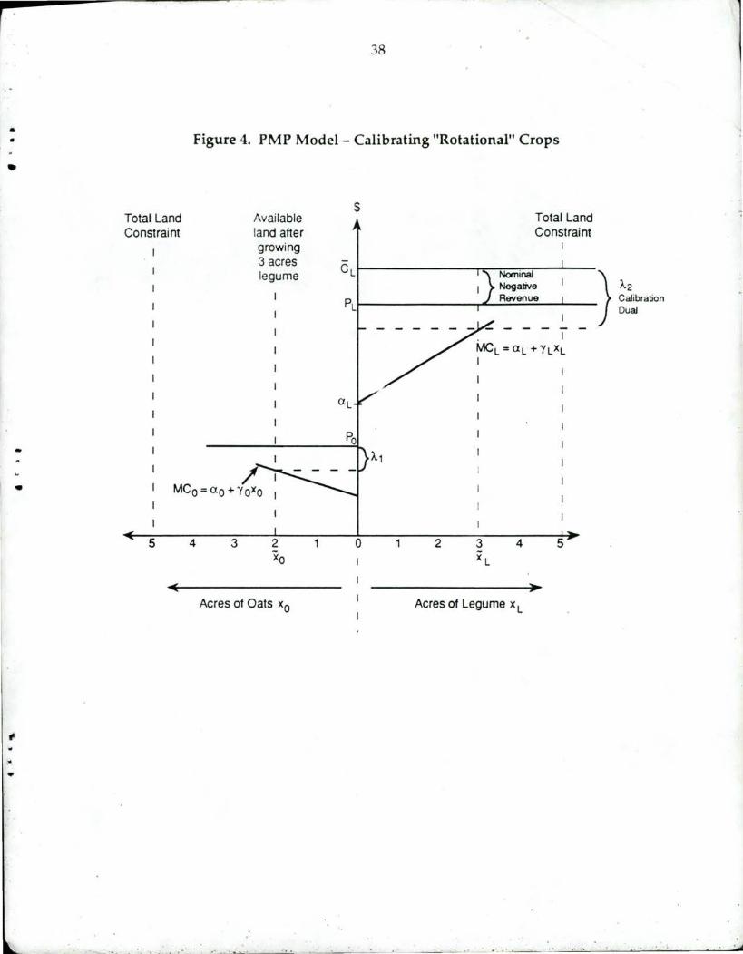
Using a simplified example shown in Figure 4, the "rotational" crop is

a legume with an observed acreage of x L· The nominal average cost per acre

is Ct and PL is the nominal revenue per acre. Since CL exceeds PL, the legume

crop appears to generate negative net revenues. Assuming similarly to

Figures 2 and 3, that the lowest positive revenue crop is oats, which sets the

opportunity cost of land at A 1, then the dual on the lower bound calibration

--- - - - - - --- ---- ---- -

23

constraint, A.2 in Figure 4, will have two components. The nominal negat ive

net revenue (PL - CL) and the opportunity cost of land A.1 .

(20)

Given the quadratic total cos t fu nction for the rotational crop xL

(21) TC= k + axL + 1/2 yxt The Marginal cost per acre is:

(22) MC= a+ yxL

Three conditions characterize the cost function for the rotational crops. First,

the marginal cost at the calibration acreage must equal the nominal cost

minus the dual value on the lower bound calibration constraint. Note that

the value of the dual is negat. . e.

(23) a+ y x = c + A.2

Second, the supply elasticity at the calibration acreage is equal to the specified

prior value 11, which implies that

(24) TlYX=a+yx

Third, the calibrated quadratic total cost function is revenue-neutral at the

calibration acreage x, implying

(25) ex = k + ax + 1 /2y x2

Equating the marginal cost condition and the elasticity condition at the

calibration acreage x we obtain:

(26)

(27)

llY x = c + A.2, solving for y we get

c + A.2 y= -

11x

Substituting this expression for y into the marginal condition results in

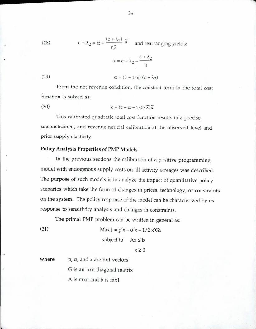
(28)

(29)

2-1

(c + A.2) -c + A.2 = a + _ x and rearranging yields:

rix

c + A.2 a=c+A.2---

Tl

From the net revenue condition, the constant term in the total cost

function is solved as:

(30) k = (c - a - 1 /2y x)x

This calibrated quadratic total cos t function results in a precise,

unconstrained, and revenue-neutral calibration at the observed level and

prior supply elasticity.

Policy Analysis Properties of PMP Models

In the previous sections the calibration of a p t) sitive programming

model with endogenous supply costs on all activity acreages was described .

The purpose of such models is to analyze the impact of quantitative policy

scenarios which take the form of changes in prices, technology, or constraints

on the system. The policy response of the model can be characterized by its

response to sensiti 0 ity analysis and changes in constraints .

(31)

where

The primal PMP problem can be written in general as:

Max J = p'x - a'x -1/2 x'Gx

subject to Ax ~ b

p, a, and x are nxl vectors

G is an nxn diagonal matrix

A is mxn and b is mxl

x~O

The revenue vector p is the product of the price and average yield as in

equations (7) and (8) . The properties of the dual values under parametric

changes to the model can be seen from the dual specification. The dual

specification of the PMP model in equation (31) is:

(32)

(33)

Min /... 1J + 1 /2 x'Gx

subject to A'/...~ p - a - Gx

A.~O

Briefly interpreted, the PMP dual problem minimizes the sum of resource

quasi rent (A.'b) and producer surplus (1 /2 x'Gx), subject to the constraint (33)

that the opportunity cost of resources used to produce each product cannot be

less than the marginal net revenue from that product.

Defining the optimal basis matrix in A to be of rank m, from the initial

PMP conditions, the number of nonzero activities is k (k>m). It follows that k

of then rows in (33) are equalities and can be written as:

(34) EA.= p - a - Gx

where E is a kxm submatrix of A, and P, a, x are kxl subvectors, and G is a kxk

diagonal matrix.

Defining the generalized inverse of E as E+, the dual values are defined

as:

(35) A. = E+(p - a - c x") .

Equation (35) shows that the dual values are linear combinations of the price

and cost parameters and the level of the nonzero activities. It follows that

parameterization of the PMP problem will result in smooth continuous

changes in all the optimal values of activity levels and dual values. This is in

contrast to LP or step-wise problems, where the dual values, and sometimes

26

the optimal solution are unchanged by parameterization unti l there is a

d iscrete change in bas is, when they jump d iscontinuously to a new level.

The ability to represent pol icies by constraint structu res is important.

The PMP formulation has the property tha t the nonlinear calibration can take

place at any level of aggregation. Tha t is, one can nes t an LP subcomponen t

within the quadra tic objectivt:. ;..inction and obtain the optimum solution to

the full problem. An example of this is used in technology selection.

Suppose a given regional commodity can oe produced by a combination of

five alternative linear technologies, whose aggregate output has a common

supply function . The PMP can calibrate the supply function while a nested LP

problem selects the set of linear technology levels that make up the aggregate

supply (Hatchett et al. 1991) .

Since the intersection of the convex sets of cons traints for the main

problem and the nested subproblem is itself convex (Marlow 1978) then the

optimal solution to the nested LP subproblem will be unchanged when the

main problem is calibrated by replacing the calibration constraints with

quadratic PMP cost functions. The calibrating functions can thus be

introduced at any level of the linear model. In some cases, the available data

on base year values will dictate the calibration level. Ideally, the level of

calibration would be determined by the properties of the cost functions, as in

the example of linear irrigation technology selection. The PMP approach does

not replace all linear cost functions with equivalent quadratic specifications,

but only replaces those that data or theory suggest are best modeled as

nonlinear .

.. 27

Conclusions

Programming models still have a strong role to play in agricultural

policy analysis, particularly for problems where time series data is absent, or

the shifts in market institutions or constraints have changed substantially

over time. The problem of calibrating programming models without

excessive constraints is addressed in this paper. The solution proposed by the

PMP approach is based on the derivation of nonlinear activity cost functions

from the base year data and prior supply elasticities . The derivation is

achieved by a simple two step procedure.

An analyst who is interested in direct applications can skip over the

derivations and calibration steps by using a menu driven program "AgMod"

(Howitt and Vayssieres 1990) . AgMod generates a GAMS program for the

model specified, and automatically runs the self cal ibra ting models, using the

GAMS/Minos optimization package. The AgMod program is available from

the authors.

The PMP approach is shown to satisfy the main criteria for calibrating

sectoral and regional models. Using PMP, the model calibrates precisely to

output and input quantities, the objective function value, and dual constraint

values and output prices. In addition, the PMP approach incorporates priors

on aggregate demand and supply elasticities.

The PMP method has been successfully used to calibrate a range of

optimization models of different size and complexity over the past eight

years. This paper has attempted to explain the economic and optimization

basis for the method, and thus broaden the discussion and exposure of the

approach among applied agricultural policy analysts . pg 7 /12/91 REH-11 .0

28

References

Bauer, S. and H . Kasnakoglu. "Non Linear Programming Models for Sector

Policy Analysis." Second International Conference on Economic

Modelling, London, March 1988.

Day, R. H. "Recursive Programming and the Production of Supply."

Agricultural Supply Functions, Heady et al., Iowa State University

Press, 1961.

Grimm, S. S., Q. Paris, and W. A. Williams. "A von Liebig Model for Water

and Nitrogen Crop Response." Western f. Agr. Econ . 12(1987):182-192.

Hatchett, S. A., G. L. Horner, and R. E. Howitt. "A Regional .Mathematical

Programming Model to Assess Drainage Control Policies." Chapter 24,

pp. 465-489. In The Economics and Managem o 1t of Water and

Drainage in Agriculture, Eds., A. Dinar and D. Zilberman. Kluwer,

1991.

Hazell P.B.R. and R. D. Norton. Mathematical Programming .for Economic

Analysis in Agriculture, MacMillan Co., New York, 1986.

House, R. M. "USMP Regional Agricultural Model. " National Economics

Division Report, Economic, Research Service, USDA, Washington,

July 1987, 30 pp.

Howitt, R. E. and M. Vayssieres. AgMod: A User's Guide. Department of

Agricultural Economics, University of California, Davis, 1990.

Just, R. E., D. Zilberman, and E. Hochman. "Estimation of Multicrop

Production Functions." Amer./. Agr. Econ. 65(1983):770-780.

29

Just, R. E., D. Zilberman, E. Hochman, and Z. Bar-Shira . "Input Allocation

Systems in Mul ticrop Systems." Amer. f. Agr. Econ. 72(1990):200-209.

Luenberger, D. G. Linear and No nlinear Programming, Addison-Wesley,

1984.

McCarl, B. A. "Cropping Activities in Agricultural Sector Models: A

Methodological Proposal. " America n Journal of Agricultural

Econom ics 64:768-771 , 1982.

Meister, A. D. , C. C. Chen, and E. 0 . Heady. Quadratic Programming Models

Applied to Agricu ltural Policies, Iowa State University Press, 1978.

Oamek G. and S. R. Johnson. "Economic and Environmental Impacts of a

Large Scale Water Transfer in the Colorado River Basin." Western

Journal of Agricu ltural Economics, forthcomi r~ . 991.

Paris, Q. and K. Knapp Estimation of von Liebig Response Functions. "

Amer.]. Agr. Econ. 71(1989):1 78-186.

Quinby, R. and D. J. Leuck. "Analysis of Selected E. C. Agricultural Policies

and Dutch Feed Composition Using Positive Mathematical

Programming. " Presented paper American Agricultural Economics

Association Annual Meeting, Knoxville, Tennessee, July 31, 1988.

Wichelns, D. and R. E. Howitt. "Price-Responsive Fixed Inputs and Fixed

Proportion Variable Inputs in Multicrop Systems." University of

Rhode Island, Department of Resource Economics Staff Paper 91-01,

32 pp., 1991.

-1

l

30

Appendix I

Proof of Constraint Decoupling

Given the degenerate problem

Problem Pl

(Al) Maximize

subject to

A

A =mxk A= (l-m)xk

f(x) - -Ax=b (I)

A A

A x<b

I x = - (II)

x = kxl k>m b = mxl A

b = (/-m)xl.

Where f(x) is monotonically increasing in x with first and second derivatives

at all points, and A is bounded and nondegenerate.

Proposition. There exists a perturbation E of the values x such that:

(a) The constraint set (I) in equation (Al) is decoupled from the

constraint set (II) in the sense that the dual values associated with

constraint set I do not depend on constraint set II.

(b) The number of binding constraints in constraint set II is reduced

so that the problem is no longer degenerate.

(c) The binding constraint set I remains unchanged.

Proof. Define the perturbed problem.

Problem P2 (A2) Maximize

subject to

f(x)

- -Ax~b (I)

A A

A x~b

I x ~ x + E (II)

I I I I I

I I I

31

A A

Any row of the nonbinding constraints Ax< b in problem Pl can be written

k A A

(A3) .I aij xi< bi i=l , ... ,(l-m) J=l

and a constraint i wi ll not become binding under the perturbation E if

k A [ k A J I ai · e· < bi - I ai · x· . 1 J J . 1 J J j= J=

(A4)

k A

Select the constraint i = 1, ... ,(/-m) such that bi - .I aij Xj is minimized. J=1

j = 1, .. . ,k are selected such that

k. [ k. J I ai · e· < bi - I ai · x· . 1 J J . 1 J J J= J=

(AS)

If Ej > 0

then no additional cons traints in the set Ax $ b will become binding under

the perturbation E.

The invariance of the binding resource constraints for the perturbation

E can be shown using the reduced gradient approach (Luenberger 1973). Using

(AS) we can w rite problem P2 using only constraint sets I and II.

(A6) Maximize f(x)

- -subject to Ax$b

Ix$x+e

where A (mxk), and I = kxk. Invoking the nondegeneracy assumption for A

and starting with the solution for problem Pl x, the constraints can be

partitioned

[: : l =b

(A7)

C:l $x5 + E

$XN + E

..,

32

where A = [B : N], B = m x m, N = m x(k-m). For brevity, we ass ume tha t the

partition of A has been made so that the (k-m) activities associated with >i

have the highest value of marginal products for the constraining resources . f rl

( i ~ i't! r .,z. IM1 t /Oex .,,,J. From Pl, the resource constraints can be written

,. '..,,! 0-" ~ (~-""'

,~~$ ~ (A8) thus,

I"'"",, ~ .(

and f(x) can be written in terms of XN, as f(B-1b - B- 1NxN, XN) the reduced

gradient for changes in x N is therefore: 1

(A9) rx =Y'L (•)-VL ( • )B-1N XN Xg

Since f( •) is monotonically increasing in XN and XB, the resource constraints

will continue to be binding since the optimization criterion will maximize

those activities with a nonnegative reduced gradient until the reduced

gradient is zero or the upper bound calibration cons traint XN +Eis

encountered. Since m<n, the model overspecializes in the more profitable

crops when subject only to constraint set I. Under the specification in

problem P2 the most profitable activities will not have a zero reduced

gradient before being constrained by the calibration set II at values of XN + £.

Thus, the binding constraint set I remains binding under the E perturbation.

The resource vector for the resource constrained crop activities (xB)

now is:

(AlO) b - N(xN + E) and from (A8)

XB = B-1[b - N(XN + £)].

Since B is of full rank m, exactly m values of XB are determined by the binding

resource constraints, which depend on the input requirements for the subset

of calibrated crop acre values XN + £.

•

33

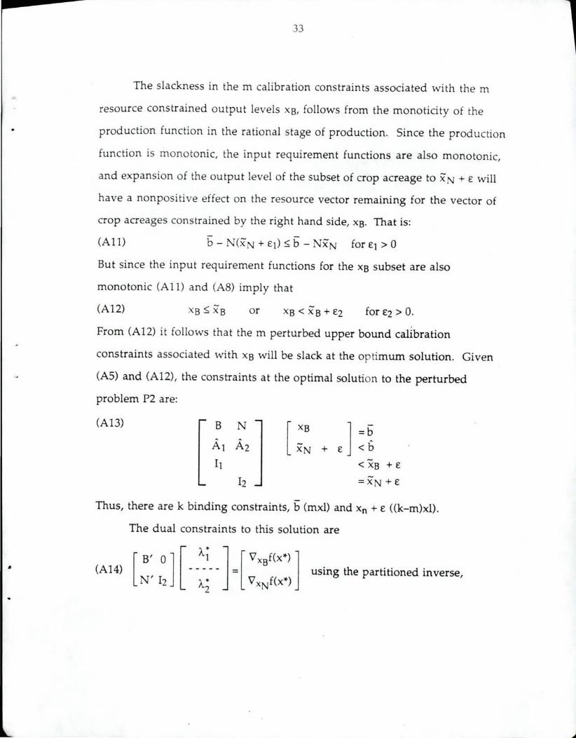
The slackness in the m calibration constraints associated with the m

resource constrained output levels xs, follows from the monoticity of the

production function in the rational stage of production. Since the production

function is monotonic, the input requirement functions are also monotonic,

and expansion of the output level of the subset of crop acreage to XN + £ will

have a nonpositive effect on the resource vector remaining for the vector of

crop acreages constrained by the right hand side, xs. That is: - -

(All) b - N(xN + £1) $ b - NxN for £1 > 0

But since the input requirement functions for the xs subset are also

monotonic (All) and (A8) imply that

(A12) or XB < Xg + £2 for £2 > 0.

From (Al2) it follows that them perturbed upper bound calibration

constraints associated with xs will be slack at the optimum solution. Given

(AS) and (A12), the constraints at the optimal solution to the perturbed

problem P2 are:

(A13) B N [ :E '] =b

A1 A2 <b XN +

11 < XB +£

12 =XN +£

Thus, there are k binding constraints, b (mxl) and Xn + £ ((k-m)xl).

The dual constraints to this solution are

using the partitioned inverse,

..

34

(AlS) OR ~! = [ P O l [ 'V x5Hx*) l 2 Q I 'V xNf(x*)

where P = B'-1 and Q = - N'B'-1.

Thus, the E perturbation on the upper bound constraint set II decouples the

dual values of constraint set I from constraint set II, and ensures that k

constraints are binding.

Footnotes to Appendix I

lA short intuitive explanation of the reduced gradient is that the net

effect of a change in x N is the gradient of the direct effect of x N on f( •) less the

effects of reductions forced on x B· The cost of reduction of xs is clearly

influenced by 'V L ( •) and the relative marginal physical products from the xs

scarce resources B-1 N .

35

Figure 1. L.P. Problem with Calibration Constraints Two Activity/One Resource Constraint

~

C>

Wheat $ calibration

Total Land Available constraint Total Land Constraint land after

!

i Constraint growing I

3acr~ wheat P.,.,

),; >-1l I I I 1 - MS-I I ~ !A?N Xw I I

/ I I Cw AC-

Xw I I

I I aw

I I

I I

I I Po

>- 1! I I

I I Co

I I

I I

_J I I .~

5 4 3 t2 0 2 3 4 5 x0 + E XW+E

Acres of Oats x 0 Acres of Wheat x w

..

..

. J

•

•

Total Land Constraint

5 4

36

Figure 2. PMP Cost Function on Wheat

Available land after growing 3 acres wheat

$

-__.;.---'------~ Co

3 0

Acres of Oats x0

Total Land Constraint

I

... ACw= aw+1 12'Yw'fw

2 4 5

Acres of Wheat x w

J

"

..

37

Figure 3. PMP Model - Quadratic Costs on all Crops

$ Total Land Available Constraint land after

growing 3 acres Pw wheat

c

MC0 =ao + Y0 x0 ~~~~_:.._~~~~-1Po

1 ACo-

5 4 3 2 0

Acres of Oats Xo

_..r--

2 3

Total Land Constraint

I

- "'AC

4 5

Acres of Wheat x w

r • •

•

-•

•

Total Land Constraint

5

38

Figure 4. PMP Model - Calibrating "Rotational" Crops

$ ~ Available Total Land

land after Constraint growing I

3 acres CL legume Nominal

) Negative A.2

pl Revenue Calibration Dual

I MCL =al + 'YLXL I

I

a l

4 3 0 2 4 5

Acres of Oats x0 Acres of Legume x L

-~~~ .. ~ • . • '--'' -~~-'-'-----'"'--"------=--:.........~-·~- -·--~--~-