The Demand for Liquid Assets: Evidence from the Minex Laurent Demand System with Conditionally Heteroscedastic Errors Dongfeng Chang School of Economics Shandong University Jinan, Shandong 250100 and Apostolos Serletis y Department of Economics University of Calgary Calgary, Alberta T3A 0Y6 Forthcoming in: Macroeconomic Dynamics October 9, 2017 This paper is based on Chapter 4 of Dongfeng Changs Ph.D. dissertation at the University of Calgary. We would like to thank Bill Barnett and the following members of Dongfengs dissertation committee: Herbert Emery, Daniel Gordon, Ron Kneebone, David Walls, and Philip Chang. y Corresponding author. Phone: (403) 220-4092; Fax: (403) 282-5262; E-mail: [email protected]; Web: http://econ.ucalgary.ca/serletis.htm. 1
Transcript
The Demand for Liquid Assets: Evidence from theMinflex Laurent Demand System with Conditionally
Heteroscedastic Errors∗
Dongfeng ChangSchool of EconomicsShandong University
Jinan, Shandong 250100and
Apostolos Serletis†
Department of EconomicsUniversity of Calgary
Calgary, Alberta T3A 0Y6
Forthcoming in: Macroeconomic Dynamics
October 9, 2017
∗This paper is based on Chapter 4 of Dongfeng Chang’s Ph.D. dissertation at the University of Calgary.We would like to thank Bill Barnett and the following members of Dongfeng’s dissertation committee:Herbert Emery, Daniel Gordon, Ron Kneebone, David Walls, and Philip Chang.†Corresponding author. Phone: (403) 220-4092; Fax: (403) 282-5262; E-mail: [email protected]; Web:
http://econ.ucalgary.ca/serletis.htm.
1
Abstract:We investigate the demand for money and the degree of substitutability among monetary
assets in the United States using the generalized Leontief and the Minflex Laurent modelsas suggested by Serletis and Shahmoradi (2007). In doing so, we merge the demand systemsliterature with the recent financial econometrics literature, relaxing the homoscedasticityassumption and instead assuming that the covariance matrix of the errors of flexible demandsystems is time-varying. We also pay explicit attention to theoretical regularity, treating thecurvature property as a maintained hypothesis. Our findings indicate that only the curvatureconstrained Minflex Laurent model with a BEKK specification for the conditional covariancematrix is able to generate inference consistent with theoretical regularity.
This paper focuses on the demand for money in the United States and investigates the degreeof substitutability among monetary assets using the flexible functional forms approach. Thisapproach, introduced by Diewert (1971), has been widely used to investigate the inter-relatedproblems of estimation of monetary asset demand functions and monetary aggregation issues.See, for example, Barnett (1983), Ewiss and Fisher (1984, 1985), Serletis and Robb (1986),Fisher and Fleissig (1994, 1997), Fleissig and Serletis (2002), and Serletis and Shahmoradi(2005, 2007), among others.As noted by Barnett (2002), the usefulness of flexible functional forms depends on whether
they satisfy the theoretical regularity conditions of positivity, monotonicity, and curvature,and in the empirical monetary demand literature there has been a tendency to ignore theo-retical regularity, as can be seen, for example, in Table 1. In this regard, as Barnett (2002,pp. 199) put it, without satisfaction of all three theoretical regularity conditions, “ . . . thesecond-order conditions for optimizing behavior fail, and duality theory fails. The resultingfirst-order conditions, demand functions, and supply functions become invalid.”Motivated by these considerations, in this paper we follow Serletis and Shahmoradi (2005,
2007) and estimate the degree of substitutability among monetary assets paying explicit at-tention to theoretical regularity, treating the curvature property as a maintained hypothesis.Furthermore, in the empirical demand systems literature, existing studies typically as-
sume that the covariance matrix of the error terms associated with the demand equationsare homoscedastic, as summarized in Table 1. In this paper we merge the demand systemsliterature with the recent financial econometrics literature by following Serletis and Isakin(2017) method to incorporate heteroscedastic variance in the demand system estimation sub-ject to full satisfaction of regularity conditions. In particular, we relax the homoscedasticityassumption and instead assume that the covariance matrix of the errors of flexible demandsystems is time-varying. By doing so, we achieve superior modeling using parametric non-linear demand systems that capture certain important features of the data.To obtain our estimates of the demand for money in the United States, we use the
monthly time series data on monetary asset quantities and their user costs recently producedby Barnett et al. (2013) and maintained within the Center of Financial Stability (CFS)program Advances in Monetary and Financial Measurement (AMFM). Our investigation isin the context of the best performed flexible functional forms in Serletis and Shahmoradi(2007): the generalized Leontief model of Diewert (1973, 1974) and the Minflex Laurentmodel introduced by Barnett (1983) and Barnett and Lee (1985). Our findings indicatethat only the curvature constrained Minflex Laurent model with a BEKK specification (seeEngle and Kroner (1995)) for the conditional covariance matrix is able to generate resultsconsistent with theoretical regularity.The rest of the paper is organized as follows. Section 2 provides a discussion of the
representative agent’s problem and Section 3 presents the two locally flexible functional
3
forms, paying explicit attention to the imposition of curvature. Section 4 discusses the datawhereas Section 5 focuses on related econometric issues and on the way to incorporate theBEKK specification for the conditional covariance matrix. Section 6 presents the empiricalresults and the final section briefly concludes the paper.
2 The Representative Agent’s Problem
We assume that the representative consumer has the following utility function
u = u(c, l,x) (1)
where c is a vector of consumption goods, l is leisure, and x is a vector of monetary assetquantities. The consumer maximizes (1) subject to the budget constraint
q′c+ wl + p′x = m
where q is a vector of prices of the consumption goods, c, w is the wage rate, p is thecorresponding vector of monetary asset user costs, and m is total income.We assume that monetary assets are as a group separable from consumption goods, c,
and leisure, l. That is, it is possible to write (1) as
u = u (c, l, f (x)) (2)
where f (x) is the aggregator function over monetary assets, x. The requirement of (direct)weak separability in x is that the marginal rate of substitution between any two componentsof x does not depend upon the values of c and l, meaning that the demand for monetaryassets is independent of relative prices outside the monetary sector – see Leontief (1947) andSono (1961). Under the weak separability assumption, we will focus on the representativeagent facing the following problem
maxxf(x) subject to p′x = y (3)
where x = (x1, x2, ..., x9) is the vector of monetary asset quantities described in Table 2,p = (p1, p2, ..., p9) is the corresponding vector of user costs, and y is the total expenditure onthe services of monetary assets. For details regarding the theory of multi-stage optimizationin the context of consumer theory, see Strotz (1957, 1959), Gorman (1959), and Blackorbyet al. (1978).Because the functional forms that we use in this paper are parameter intensive, we face
the problem of having a large number of parameters in estimation. To reduce the numberof parameters, we follow Serletis and Shahmoradi (2007) and separate the group of assets
4
into three collections based on empirical pretesting. Thus the monetary utility function in(3) can be written as
)where the subaggregate functions fi (i = A,B,C) provide subaggregate measures of mone-tary services.Instead of using the simple-sum index, currently in use by the Federal Reserve and most
central banks around the world, to construct the monetary subaggregates, fi (i = A, B, C),we follow Barnett (1980) and use the Divisia quantity index to allow for less than perfectsubstitutability among the relevant monetary components. The Divisia index (in discretetime) is defined as
logMDt − logMD
t−1 =n∑j=1
s∗jt(log xjt − log xjt−1)
according to which the growth rate of the aggregate is the weighted average of the growthrates of the component quantities, with the Divisia weights being defined as the expenditureshares averaged over the two periods of the change, s∗jt = (1/2)(sjt + sj,t−1) for j = 1, ..., n,where sjt = πjtxjt/πktxkt is the expenditure share of asset j during period t , and πjt is thenominal user cost of asset j, derived in Barnett (1978),
πjt = p∗tRt − rjt1 +Rt
which is just the opportunity cost of holding a dollar’s worth of the jth asset. Above, p∗tis the true-cost-of-living index, rjt is the market yield on the jth asset, and Rt is the yieldavailable on a benchmark asset that is held only to carry wealth between multiperiods.
3 Flexible Demand Systems
In this section we briefly discuss the generalized Leontief (GL) and the Minflex Laurent (ML)models that we use to approximate the unknown underlying indirect utility function of therepresentative economic agent as well as the procedure of imposing the curvature conditionsin each model. Both models are locally flexible and capable of approximating any unknownfunction up to the second order.
5
3.1 The Generalized Leontief
According to Diewert (1974), the generalized Leontief flexible functional form has the fol-lowing reciprocal indirect utility function
h(v) = a0 +
n∑i=1
aiv1/2i +
1
2
n∑i=1
n∑j=1
βijvivj (4)
where v = [v1, v2, ..., vn] is a vector of income normalized user costs with vi = pi/y, wherepi is the user cost of asset i and y is the total expenditure on the n assets. B = [βij] is ann × n symmetric matrix of parameters and a0 and ai are other parameters, for a total of(n2 + 3n+ 2)/2 parameters. The GL share equations, derived using the logarithmic form ofRoy’s identity are
si =
aiv1/2i +
n∑j=1
βijv1/2i v
1/2j
n∑j=1
ajv1/2j +
n∑k=1
n∑m=1
βkmv1/2k v
1/2m
, i = 1, ..., n. (5)
Since the share equations are homogenous of degree zero in the parameters, we followBarnett and Lee (1985) and impose the following normalization in estimation:
2n∑i=1
ai +n∑i=1
n∑j=1
βij = 1. (6)
Curvature condition of the GL reciprocal indirect utility function requires the Hessianmatrix to be negative semidefinite. Local curvature can be imposed using the Serletis andShahmoradi (2007) procedure by evaluating the Hessian terms of (4) at v∗= 1, as follows,
Hij = −δij
(ai +
n∑j=1, j 6=i
βij
)+ (1− δij) βij
where δij is the Kronecker delta (that is, δij = 1 when i = j and 0 otherwise).Replacing H with −KK ′, where K is an n× n lower triangular matrix so that −KK ′
is by construction a negative semidefinite matrix. The above can be written as
− (KK ′)ij = −δij
(ai +
n∑j=1, j 6=i
βij
)+ (1− δij) βij (7)
Solving for the ai and βij terms as a function of the (KK ′)ij , we can get the restrictionsthat ensure the negative semidefiniteness of the Hessian matrix.
6
In particular, when i 6= j , equation (7) implies that
βij = − (KK ′)ij (8)
and when i = j, it implies that
(KK ′)ii = ai +n∑
j=1, j 6=i
βij.
Substituting βij from (8) into the above equation, we get
ai =n∑j=1
(KK ′)ij . (9)
for i, j = 1, ..., n. See Serletis and Shahmoradi (2007) for an example with n = 3.
3.2 The Minflex Laurent Model
The Minflex Laurent (ML) model, introduced by Barnett (1983) and Barnett and Lee (1985),is a special case of the Full Laurent model also introduced by Barnett (1983). FollowingBarnett (1983), the Full Laurent reciprocal indirect utility function is
h(v) = a0 + 2n∑i=1
aiv1/2i +
n∑i=1
n∑j=1
aijv1/2i v
1/2j − 2
n∑i=1
biv−1/2i −
n∑i=1
n∑j=1
bijv−1/2i v
−1/2j (10)
where a0, ai, aij, bi, and bij are unknown parameters and vi denotes the income normalizedprice, pi/y.By assuming that bi = 0, bii = 0 ∀i, aijbij = 0 ∀i, j, and forcing the off diagonal elements
of the symmetric matrices A ≡ [aij] and B ≡ [bij] to be nonnegative, (10) reduces to theML reciprocal indirect utility function
h(v) = a0 + 2n∑i=1
aiv1/2i +
n∑i=1
aiivi +n∑i=1
n∑j=1
i 6=j
a2ijv1/2i v
1/2j −
n∑i=1
n∑j=1
i 6=j
b2ijv−1/2i v
−1/2j (11)
Note that the off diagonal elements of A and B are nonnegative as they are raised to thepower of two.By applying Roy’s identity to (11), the share equations of the ML demand system are
si =
aiv1/2i + aiivi +
n∑j=1
i 6=j
a2ijv1/2i v
1/2j +
n∑j=1
i 6=j
b2ijv−1/2i v
−1/2j
n∑i=1
aiv1/2i +
n∑i=1
aiivi +n∑i=1
n∑j=1
i 6=j
a2ijv1/2i v
1/2j +
n∑i=1
n∑j=1
i 6=j
b2ijv−1/2i v
−1/2j
(12)
7
Since the share equations are homogenous of degree zero in the parameters, we follow Barnettand Lee (1985) and impose the following normalization in the estimation of (12)
n∑i=1
aii + 2
n∑i=1
ai +
n∑j=1
i 6=j
a2ij −n∑j=1
i 6=j
b2ij = 1 (13)
Hence, there are
1 + n+n(n+ 1)
2+n(n− 1)
2
parameters in (11), but the n (n− 1) /2 equality restrictions, aijbij = 0 ∀i, j, and the nor-malization (13) reduce the number of parameters in equation (12) to (n2 + 3n) /2.As shown by Barnett (1983, Theorem A.3), (11) is globally concave for every v ≥ 0, if all
parameters are nonnegative, as in that case (11) would be a sum of concave functions. If theinitially estimated parameters of the vector a and matrix A are not nonnegative, curvaturecan be imposed globally by replacing each unsquared parameter by a squared parameter, asin Barnett (1983).
4 Data
We use monthly data on monetary asset quantities and their user costs for the nine itemslisted in Table 2, recently produced by Barnett et al. (2013) and maintained within the Cen-ter of Financial Stability (CFS) program Advances in Monetary and Financial Measurement(AMFM). The sample period is from 1967:1 to 2015:3 (a total of 579 observations). Fora detailed discussion of the data and the methodology of the calculation of user costs, seeBarnett et al. (2013) and http://www.centerforfinancialstability.org. As we require real percapita asset quantities for our empirical work, we have divided each measure of monetaryservices by the U.S. CPI (all items) and total U.S. population in each period.Because demand system estimation requires heavy dimension reduction (as already noted
in Section 2), we use the Divisia index to reduce the dimension of each model by constructingthe three subaggregates shown in Table 2. In particular, subaggregate A (M1) is composedof currency, traveler’s checks, and other checkable deposits, including Super NOW accountsissued by commercial banks and thrifts (series 1 to 5 in Table 2). Subaggregate B (Savingsdeposits) is composed of savings deposits issued by commercial banks and thrifts (series 6and 7), and subaggregate C (Time deposits) is composed of small time deposits issued bycommercial banks and thrifts (series 8 and 9). Divisia user cost indices for each of thesesubaggregates are calculated by applying Fisher’s (1922) weak factor reversal test.
8
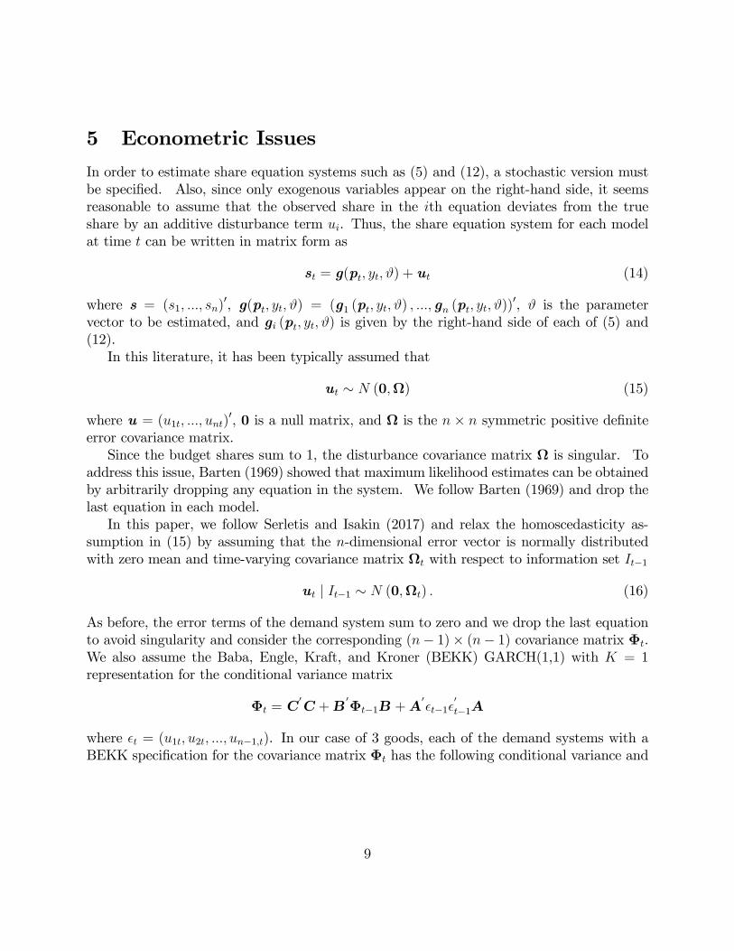
5 Econometric Issues
In order to estimate share equation systems such as (5) and (12), a stochastic version mustbe specified. Also, since only exogenous variables appear on the right-hand side, it seemsreasonable to assume that the observed share in the ith equation deviates from the trueshare by an additive disturbance term ui. Thus, the share equation system for each modelat time t can be written in matrix form as
st = g(pt, yt, ϑ) + ut (14)
where s = (s1, ..., sn)′, g(pt, yt, ϑ) = (g1 (pt, yt, ϑ) , ..., gn (pt, yt, ϑ))
′, ϑ is the parametervector to be estimated, and gi (pt, yt, ϑ) is given by the right-hand side of each of (5) and(12).In this literature, it has been typically assumed that
ut ∼ N (0,Ω) (15)
where u = (u1t, ..., unt)′, 0 is a null matrix, and Ω is the n × n symmetric positive definite
error covariance matrix.Since the budget shares sum to 1, the disturbance covariance matrix Ω is singular. To
address this issue, Barten (1969) showed that maximum likelihood estimates can be obtainedby arbitrarily dropping any equation in the system. We follow Barten (1969) and drop thelast equation in each model.In this paper, we follow Serletis and Isakin (2017) and relax the homoscedasticity as-
sumption in (15) by assuming that the n-dimensional error vector is normally distributedwith zero mean and time-varying covariance matrix Ωt with respect to information set It−1
ut | It−1 ∼ N (0,Ωt) . (16)
As before, the error terms of the demand system sum to zero and we drop the last equationto avoid singularity and consider the corresponding (n− 1)× (n− 1) covariance matrix Φt.We also assume the Baba, Engle, Kraft, and Kroner (BEKK) GARCH(1,1) with K = 1representation for the conditional variance matrix
Φt = C′C +B
′Φt−1B +A
′εt−1ε
′
t−1A
where εt = (u1t, u2t, ..., un−1,t). In our case of 3 goods, each of the demand systems with aBEKK specification for the covariance matrix Φt has the following conditional variance and
See Serletis and Isakin (2017) for a detailed discussion. All estimations are performed inEstima RATS.
6 Empirical Evidence
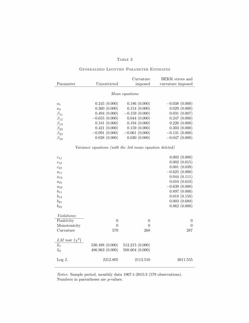
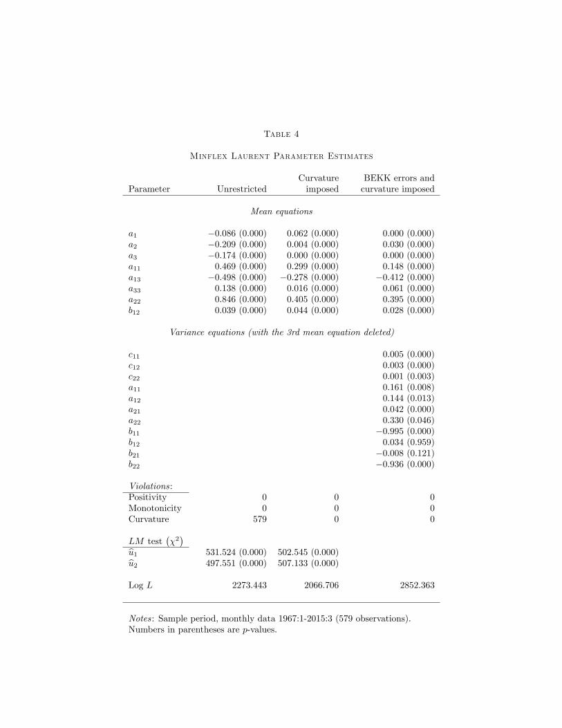
In Tables 3 and 4 we report a summary of results from the generalized Leontief and Min-flex Laurent models in terms of parameter estimates (with p-values in parentheses) for themean equations (5) and (12), and the variance equations (17). We also report positivity,monotonicity, and curvature violations, Lagrange Multiplier test results for ARCH effects, aswell as log likelihood values, when the models are estimated without the curvature conditionsimposed (in the first column), with the curvature conditions imposed (in the second column),and with both BEKK errors and curvature conditions imposed (in the last column).As can be seen in the first column of Tables 3 and 4, both models satisfy positivity and
monotonicity at all sample observations when the curvature conditions are not imposed, butboth unrestricted models violate curvature when curvature is not imposed. Because regu-larity has not been attained (by luck), we follow Barnett (2002) and estimate the modelsby imposing the curvature conditions, using the methodology discussed in Section 3. Theresults are disappointing in the case of the GL model. As can be seen in the second column ofTable 3, the imposition of local curvature on the GL model reduces the number of curvatureviolations, but does not completely eliminate them. Only the curvature restricted MinflexLaurent model satisfies full theoretical regularity (see the second column of Table 4). More-over, when we relax the homoscedasticity assumption and model the curvature constraineddemand systems with the BEKK GARCH(1,1) errors specification, we find that only thecurvature constrained Minflex Laurent model with BEKK errors satisfies all three regularityconditions at all data points (see the last column of Tables 3 and 4).To verify that homoscedasticity is not a good assumption in this literature, we report χ2
statistics of Lagrange Multiplier tests for the models estimated under the homoscedasticity
10
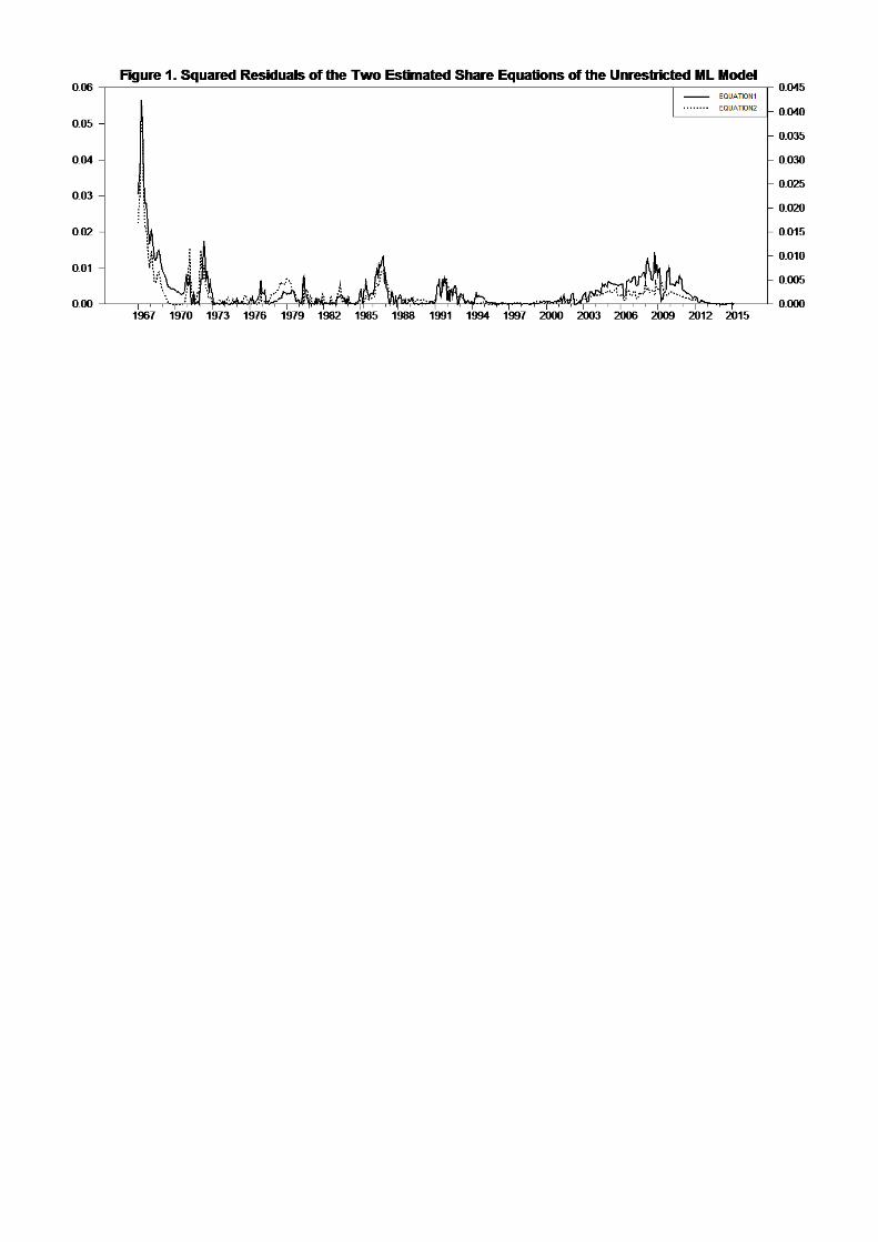
assumption (see the first and second columns) in Tables 3 and 4. Results show statisticallysignificant evidence of ARCH effects when the models are estimated under the homoscedas-ticity assumption. This is also supported by the plots of the estimated squared residuals,u21 and u
22, of the unrestricted and curvature restricted Minflex Laurent model in Figures 1
and 2, respectively; similar figures for the GL model are available upon request. Overall,based on our evidence, only the curvature constrained Minflex Laurent model with a BEKKspecification for the conditional variance matrix is able to provide inference that is consistentwith full theoretical regularity and the time series properties of the data.In the demand systems approach to the estimation of economic relationships, the primary
interest, especially in policy analysis, is in how the arguments of the underlying functionaffect the quantities demanded. This is conventionally expressed in terms of the income andprice elasticities and the Allen and Morishima elasticities of substitution. These elasticitiescan be calculated from the estimated budget share equations by writing the left-hand sideas
xi =siy
pi, i = 1, ..., n.
In particular, the income elasticities can be calculated by
ηiy = 1 +y
si
∂si∂y, i = 1, ..., n
and the Marshallian (or uncompensated) price elasticities by
ηij =pjsi
∂si∂pj− δij, i, j = 1, ..., n
where δij is the Kronecker delta (that is, δij = 1 when i = j and 0 otherwise). The Allen(1938) elasticities of substitution can be calculated by
σaij = ηiy +ηjisi= σaji, i, j = 1, ..., n
and the Morishima (1967) elasticities of substitution by
σmij = si(σaji − σaii), i, j = 1, ..., n.
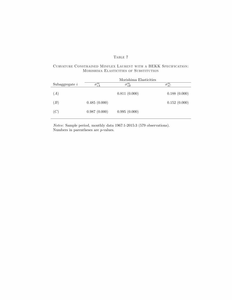
We report the income and the own- and cross-price elasticities evaluated at the mean ofthe data (with p-values in parentheses) in Table 5, the Allen elasticities of substitution inTable 6, and the Morishima elasticities of substitution in Table 7. We do so for each of thethree monetary subaggregates, A, B, and C, and only for the curvature constrained MinflexLaurent model with a BEKK specification for the conditional variance matrix, since thisis the only model that satisfies full theoretical regularity and reflects the data generating
11
process. Since the elasticities are functions of the parameter estimates, we construct thereported standard errors using the Delta method.As expected, all the income elasticities reported in Table 5, ηA, ηB, and ηC , are positive
and statistically significant (ηA = 1.171 with a p-value of 0.000, ηB = 0.864 with a p-value of0.000, and ηC = 2.304 with a p-value of 0.000), implying that M1 (A), savings deposits (B),and time deposits (C) are all normal goods, which is consistent with economic theory and theexisting literature. The own-price elasticities, ηii, are all negative, as predicted by the theory,and statistically significant (ηAA = −0.988 with a p-value of 0.000, ηBB = −0.639 with ap-value of 0.000, and ηCC = −1.015 with a p-value of 0.000). For the cross-price elasticities,ηij, economic theory does not predict any signs, but we note that the off-diagonal terms inTable 5 are negative, indicating that the assets taken as a whole are gross complements.This is (qualitatively) consistent with the evidence reported by Serletis and Shahmoradi(2005) using the Fourier and AIM globally flexible functional forms and that by Serletis andShahmoradi (2007) using the Minflex Laurent and generalized Leontief models.In addition to the standard Marshallian income and price elasticities, we show estimates
of the Allen elasticities of substitution in Table 6, evaluated at the means of the data. Asexpected, the three diagonal terms of the Allen own elasticities of substitution for the threeassets are negative (σaAA = −1.944 with a p-value of 0.000, σaBB = −1.697 with a p-value of0.000, and σaCC = −8.840 with a p-value of 0.000). However, because the Allen elasticityof substitution produces ambiguous results off diagonal, we use the Morishima elasticity ofsubstitution to investigate the substitutability/complementarity relationship between mon-etary assets– see Blackorby and Russell (1989) for more details. Based on the Morishimaelasticities of substitution shown in Table 7, the assets are Morishima substitutes, with allMorishima elasticities of substitution being less than unity.
7 Comparison with Other Studies
It is diffi cult to provide a comparison between our results and those obtained in previousstudies using different flexible functional forms and different monetary assets. Moreover,as we have already mentioned, most of the money demand studies listed in Table 1 do notproduce inference consistent with neoclassical microeconomic theory, and all of the studieslisted in Table 1 are based on the homoscedasticity assumption.Our results, however, are generally consistent with those reported by Serletis and Shah-
moradi (2007) who investigate the same monetary assets using the Minflex Laurent modelas we do in this paper. That is, the monetary assets are Morishima substitutes, with allthe Morishima elasticities of substitution being less than unity. This is evidence againstwhat Barnett (2016) refers to as the ‘Linearity Condition,’which requires infinite elasticitiesof substitution. It is also consistent with much of the earlier literature that was based ondifferent demand systems and different monetary assets. It means that the simple-sum mon-
12
etary aggregates used by the Federal Reserve (and other central banks around the world) areinconsistent with neoclassical microeconomic theory, and therefore should be abandoned.
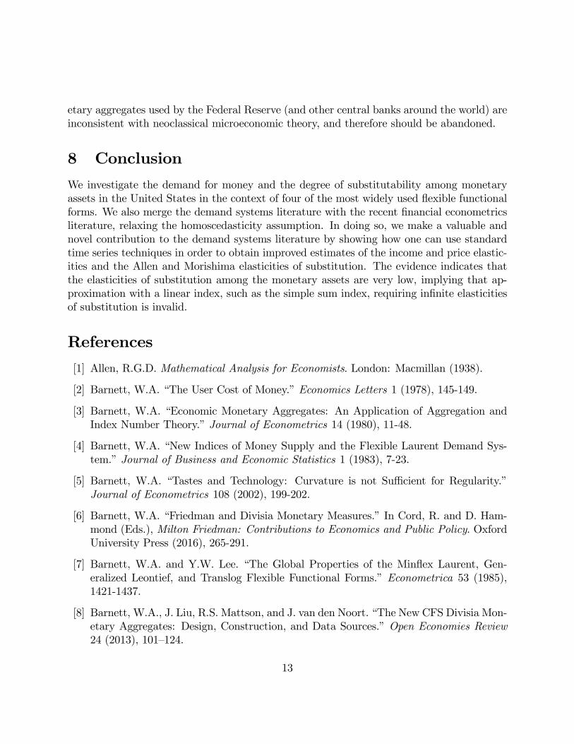
8 Conclusion
We investigate the demand for money and the degree of substitutability among monetaryassets in the United States in the context of four of the most widely used flexible functionalforms. We also merge the demand systems literature with the recent financial econometricsliterature, relaxing the homoscedasticity assumption. In doing so, we make a valuable andnovel contribution to the demand systems literature by showing how one can use standardtime series techniques in order to obtain improved estimates of the income and price elastic-ities and the Allen and Morishima elasticities of substitution. The evidence indicates thatthe elasticities of substitution among the monetary assets are very low, implying that ap-proximation with a linear index, such as the simple sum index, requiring infinite elasticitiesof substitution is invalid.
References
[1] Allen, R.G.D. Mathematical Analysis for Economists. London: Macmillan (1938).
[2] Barnett, W.A. “The User Cost of Money.”Economics Letters 1 (1978), 145-149.
[3] Barnett, W.A. “Economic Monetary Aggregates: An Application of Aggregation andIndex Number Theory.”Journal of Econometrics 14 (1980), 11-48.
[4] Barnett, W.A. “New Indices of Money Supply and the Flexible Laurent Demand Sys-tem.”Journal of Business and Economic Statistics 1 (1983), 7-23.
[5] Barnett, W.A. “Tastes and Technology: Curvature is not Suffi cient for Regularity.”Journal of Econometrics 108 (2002), 199-202.
[6] Barnett, W.A. “Friedman and Divisia Monetary Measures.”In Cord, R. and D. Ham-mond (Eds.), Milton Friedman: Contributions to Economics and Public Policy. OxfordUniversity Press (2016), 265-291.
[7] Barnett, W.A. and Y.W. Lee. “The Global Properties of the Minflex Laurent, Gen-eralized Leontief, and Translog Flexible Functional Forms.”Econometrica 53 (1985),1421-1437.
[8] Barnett, W.A., J. Liu, R.S. Mattson, and J. van den Noort. “The New CFS Divisia Mon-etary Aggregates: Design, Construction, and Data Sources.”Open Economies Review24 (2013), 101—124.
13
[9] Barten, A.P. “Maximum Likelihood Estimation of a Complete System of Demand Equa-tions.”European Economic Review 1 (1969), 7-73.
[10] Blackorby, C., D. Primont, and R.R. Russell. Duality, Separability, and FunctionalStructure. Amsterdam: North-Holland (1978).
[11] Blackorby, C., D. Primont, and R.R. Russell. “Will the Real Elasticity of SubstitutionPlease Stand Up?”American Economic Review 79 (1989), 882-888.
[12] Diewert, W.E. “An Application of the Shephard Duality Theorem: A Generalized Leon-tief Production Function.”Journal of Political Economy 79 (1971), 481-507.
[13] Diewert, W.E. “Functional Forms for Profit and Transformation Functions.”Journal ofEconomic Theory 6 (1973), 284-316.
[14] Diewert, W.E. “Applications of Duality Theory.” In M. Intriligator and D. Kendrick(eds.), Frontiers in Quantitive Economics. Amsterdam: North-Holland (1974), 106-171.
[15] Drake, L. and A.R. Fleissig. “Semi-Nonparametric Estimates of Currency Substitution:The Demand for Sterling in Europe.”Review of International Economics 12 (2004),374-394.
[16] Drake, L. and A.R. Fleissig. “Substitution between Monetary Assets and ConsumerGoods: New Evidence on the Monetary Transmission Mechanism.”Journal of Bankingand Finance 34 (2010), 2811-2821.
[17] Drake, L., A.R. Fleissig, and A. Mullineaux. “Are ‘Risky’Assets Substitutes for ‘Mon-etary Assets’? Evidence from an AIM Demand System.”Economic Inquiry 37 (1999),510-526.
[18] Drake, L., A.R. Fleissig, and J.L. Swofford. “A Seminonparametric Approach to theDemand for U.K. Monetary Assets.”Economica 70 (2003), 99-120.
[19] Engle, R.F. and K.F. Kroner. “Multivariate Simultaneous Generalized ARCH.”Econo-metric Theory 11 (1995), 122-150.
[20] Ewiss, N.A. and D. Fisher. “The Translog Utility Function and the Demand for Moneyin the United States.”Journal of Money, Credit and Banking 16 (1984), 34-52.
[21] Ewiss, N.A. and D. Fisher. “Toward a Consistent Estimate of the Substitutability be-tween Money and Near Monies: An Application of the Fourier Flexible Form.”Journalof Macroeconomics 7 (1985), 151-174.
14
[22] Fisher, D. and A.R. Fleissig. “Money Demand in a Flexible Dynamic Fourier Expendi-ture System.”Federal Reserve Bank of St. Louis Review 76 (1994), 117-128.
[23] Fisher, D. and A.R. Fleissig. “Monetary Aggregation and the Demand for Assets.”Journal of Money, Credit and Banking 29 (1997), 458-475.
[24] Fisher, I. The Making of Index Numbers: A Study of Their Varieties, Tests, and Relia-bility. Boston: Houghton Miffl in (1922).
[25] Fleissig, A.R. “The Dynamic Laurent Flexible Form and Long-Run Analysis.”Journalof Applied Econometrics 12 (1997), 687-699.
[26] Fleissig, A.R. and A. Serletis. “Seminonparametric Estimates of Substitution for Cana-dian Monetary Assets.”Canadian Journal of Economics 35 (2002), 78-91.
[27] Fleissig, A.R. and J.L. Swofford. “A Dynamic Asymptotically Ideal Model of MoneyDemand.”Journal of Monetary Economics 37 (1996), 371-380.
[28] Gorman, W.M. “Separable Utility and Aggregation.”Econometrica 27 (1959), 469-481.
[29] Leontief, W.W. “An Introduction to a Theory of the Internal Structure of FunctionalRelationships.”Econometrica 15 (1947), 361-373.
[30] Morishima, M. “A Few Suggestions on the Theory of Elasticity (in Japanese).”KeizaiHyoron (Economic Review) 16 (1967), 144-150.
[31] Serletis, A. “The Demand for Divisia M1, M2, and M3 in the United States.”Journalof Macroeconomics 9 (1987), 567-591.
[32] Serletis, A. “Translog Flexible Functional Forms and Substitutability of Monetary As-sets.”Journal of Business and Economic Statistics 6 (1988), 59-67.
[33] Serletis, A. and G. Feng. “Semi-Nonparametric Estimates of Currency SubstitutionBetween the Canadian Dollar and the U.S. Dollar.”Macroeconomic Dynamics 14 (2010),29-55.
[34] Serletis, A. and M. Isakin. “Stochastic Volatility Demand Systems.”Econometric Re-views 36 (2017), 1111-1122.
[35] Serletis, A. and A.L. Robb. “Divisia Aggregation and Substitutability among MonetaryAssets.”Journal of Money, Credit, and Banking 18 (1986), 430-446.
[36] Serletis, A. and A. Shahmoradi. “Semi-Nonparametric Estimates of the Demand forMoney in the United States.”Macroeconomic Dynamics 9 (2005), 542-559.
15
[37] Serletis, A. and A. Shahmoradi. “Flexible Functional Forms, Curvature Conditions, andthe Demand for Assets.”Macroeconomic Dynamics 11 (2007), 455-486.
[38] Sono, M. “The Effect of Price Changes on the Demand and Supply of Separable Goods.”International Economic Review 2 (1961), 239-271.
[39] Strotz, R.H. “The Empirical Implications of a Utility Tree.”Econometrica 25 (1957),169-180.
[40] Strotz, R.H. “The Utility Tree-A Correction and Further Appraisal.”Econometrica 27(1959), 482-488.
16
Table 1
A summary of flexible functional forms estimation of monetary assets demand
Curvature HomoscedasticityAuthor(s) Model used imposed assumed
Barnett (1983) Minex Laurent X XEwis and Fisher (1984) Translog XEwis and Fisher (1985) Fourier XSerletis and Robb (1986) Translog XSerletis (1987, 1988) Translog XFisher and Fleissig (1994, 1997) Fourier XFleissig (1997) Minex, GL, Translog XFleissig and Swoord (1996) AIM XDrake, Fleissig, and Mullineux (1999) AIM XFleissig and Serletis (2002) Fourier XDrake, Fleissig, and Swoord (2003) AIM XDrake and Fleissig (2004) Fourier XSerletis and Shahmoradi (2005) AIM and Fourier X XSerletis and Shahmoradi (2007) GL, BTL, AIDS, Minex, NQ X XDrake and Fleissig (2010) Fourier XSerletis and Feng (2010) AIM X X
Table 2
Monetary Assets/Components
A:1 Currency2 Travelers checks3 Demand deposits4 Other checkable deposits at banks including Super Now accounts5 Other checkable deposits at thrifts including Super Now accounts
B:6 Savings deposits at banks including money market deposit accounts7 Savings deposits at thrifts including money market deposit accounts
C:8 Small denomination time deposits at commercial banks9 Small denomination time deposits at thrift institutions