+ All Categories
Home > Documents > Department - Massachusetts Institute of Technology

Department - Massachusetts Institute of Technology

Date post: 16-Oct-2021
Category:
Upload: others
View: 3 times
Download: 0 times
Share this document with a friend
154
INCREMENTAL SYNTHESIS OF OPTIMAL CONTROL LAWS USING LEARNING ALGORITHMS Stephen C. Atkins S.B. Aeronautics and Astronautics Massachusetts Institute of Technology (1991) SUBMITTED TO THE DEPARTMENT OF AERONAUTICS AND ASTRONAUTICS IN PARTIAL FULFILLMENT OF THE REQUIREMENTS FOR THE DEGREE OF MASTER OF SCIENCE in AERONAUTICS AND ASTRONAUTICS at the MASSACHUSETTS INSTITUTE OF TECHNOLOGY May, 1993 @Stephen C. Atkins, 1993, All Rights Reserved Signature of Author Approved by /Department of Aeronautics and Astronautics May 7, 1993 Walter L. Baker Technical Supervisor, C. S. Draper Laboratory Certified by U..v Professor Wallace E. Vander Velde A Thesis Supervisor Accepted by 111- - ... .. Pofessor Marokd Y Wachman Chairman, Department Graduate Committee Aero MASSACHUSETTS INSTITUTE OF TECHN nnv JUN1 08 1993 - -
Transcript

INCREMENTAL SYNTHESIS OF OPTIMAL CONTROL LAWS

USING LEARNING ALGORITHMS

Stephen C. Atkins

S.B. Aeronautics and AstronauticsMassachusetts Institute of Technology

(1991)

SUBMITTED TO THE DEPARTMENT OF AERONAUTICS AND ASTRONAUTICSIN PARTIAL FULFILLMENT OF THE REQUIREMENTS FOR THE DEGREE OF

MASTER OF SCIENCE

in

AERONAUTICS AND ASTRONAUTICS

at the

MASSACHUSETTS INSTITUTE OF TECHNOLOGY

May, 1993

@Stephen C. Atkins, 1993, All Rights Reserved

Signature of Author

Approved by

/Department of Aeronautics and AstronauticsMay 7, 1993

Walter L. BakerTechnical Supervisor, C. S. Draper Laboratory

Certified by U..v

Professor Wallace E. Vander VeldeA Thesis Supervisor

Accepted by 111- -

... .. Pofessor Marokd Y WachmanChairman, Department Graduate Committee

AeroMASSACHUSETTS INSTITUTE

OF TECHN nnv

JUN1 08 1993i anaoRIFS

- -

INCREMENTAL SYNTHESIS OF OPTIMAL CONTROL LAWSUSING LEARNING ALGORITHMS

Stephen C. Atkins

Submitted to the Department of Aeronautics and Astronauticsat the Massachusetts Institute of Technology

on May 7, 1993 in partial fulfillment of the requirements for thedegree of Master of Science in Aeronautics and Astronautics

ABSTRACT

Learning systems represent an approach to optimal control law design forsituations where initial model uncertainty precludes the use of robust, fixed controllaws. This thesis analyzes a variety of techniques for the incremental synthesisof optimal control laws, where the descriptor incremental implies that an on-lineimplementation filters the information acquired through real-time interactions withthe plant and the operating environment. A direct/indirect framework is proposedas a means of classifying approaches to learning optimal control laws. Within thisframework, relationships among existing direct algorithms are examined, and aspecific class of indirect control laws is developed.

Direct learning control implies that the feedback loop that motivates the learn-ing process is closed around system performance. Reinforcement learning is a type ofdirect learning technique with origins in the prediction of animal learning phenom-ena that is largely restricted to discrete input and output spaces. Three algorithmsthat employ the concept of reinforcement learning are presented: the AssociativeControl Process, Q learning, and the Adaptive Heuristic Critic.

Indirect learning control denotes a class of incremental control law synthesismethods for which the learning loop is closed around the system model. The ap-proach discussed in this thesis integrates information from a learned mapping of theinitially unmodeled dynamics into finite horizon optimal control laws. Therefore,the derivation of the control law structure as well as the closed-loop performanceremain largely external to the learning process. Selection of a method to approxi-mate the nonlinear function that represents the initially unmodeled dynamics is aseparate issue not explicitly addressed in this thesis.

Dynamic programming and differential dynamic programming are reviewedto illustrate how learning methods relate to these classical approaches to optimalcontrol design.

The aeroelastic oscillator is a two state mass-spring-dashpot system excitedby a nonlinear lift force. Several learning control algorithms are applied to theaeroelastic oscillator to either regulate the mass position about a commanded pointor to track a position reference trajectory; the advantages and disadvantages ofthese algorithms are discussed.

Thesis Supervisor: Professor Wallace E. Vander VeldeTitle: Department of Aeronautics and Astronautics

Technical Supervisor: Walter L. BakerTitle: Senior Member of Technical Staff, C. S. Draper Laboratory

Acknowledgments

Love and appreciation to Mom and Dad (proper nouns?) for a lifetime ofattention, support, encouragement, and no pressure - well, maybe a little pressurein the beginning. I don't think I can express how grateful I am, and I probably willnot fully realize the importance of your commitment for many years, but I thinkyou know how I feel.

To brother Bob... thanks for leaving me alone as an undergraduate so thatI could learn to stop following in your footsteps. I've learned a lot from you and Ihope that I've taught you something, too. Congratulations on finally getting out ofthis place. Remember, getting everything you want in life is more important thanwinning!

Heather - thanks for years of emotional stability. I wished we were closer,but the friendship was great; and now after 71 years, what a misguided thing tolet happen. Have a wonderful life.

Walt Baker, I am obliged to you for the frequent guidance and technical as-sistance - even though we seem to think about everything a bit differently. Youhave been an excellent supervisor, football defensive lineman, and friend.

I appreciate the efforts of Professor VanderVelde, a very busy man, for care-fully reviewing my work.

Additionally, Pete Millington enthusiastically offered to give me some adviceif he ever has time... Pete, when we did talk, you always painted clear picturesPete is cool of what was important, thanks.

I acknowledge Harry Klopf, Jim Morgan, and Leemon Baird for giving me agood place whence to start.

I thank Mario Santarelli and the rest of the SimLab team for opening the door(twice).

Equally significant were the distractions, I mean the friends, who seldom al-lowed the past six years to get boring. Noel - I miss Kathy's cooking as well asthe competition of Nerf basketball games. I hope you get the aircraft you want.Thanks to everyone for making Draper a fun place to tool: Ruth, Dean, Tom(s),

6 Acknowledgments

Kortney, Bill, Ching, Roger, Eugene, Steve, Torsten, Dan, Mitch, Dino, etc... andthe same to the crowd who never understood why I was always at Draper: Jim,Kim, Jane, and Christine.

Jabin - 8.01 was so long ago! I never thought that you would get marriedbefore me; best wishes for the future. Thanks for all the random conversations andI hope you get a chance to put a hockey stick in orbit someday.

To J3/DC (Ojas, Ajit, Pat, Adrian, Hugo, Geno, and Trini), thanks for thecamaraderie. King - I'll see you in Sydney. Dave, Deb, Sanjeev, Tamal, Art, Pete,Chuck, Jason, Brent, Steve - thanks for always being there.

This thesis was prepared at the Charles Stark Draper Laboratory, Inc. with supportprovided by the U. S. Air Force Wright Laboratory under Contract F33615-88-C-1740. Publication of this report does not constitute approval by C. S. DraperLaboratory or the sponsoring agency of the findings or conclusions contained herein.This thesis is published for the exchange and stimulation of ideas.

The author reserves the right to reproduce and distribute this thesis document inwhole or in part.

I hereby grant permission to reproduce and distribute this thesis document, in wholeor in part, to the Massachusetts Institute of Technology, Cambridge, MA.

I hereby assign my copyright of this thesis to The Charles SIrk Draper La ratory,Inc., Cambridge, MA. (2 // 1-7 // I

Table of Contents

Abstract . . . . . . . . .

Acknowledgments .........

Table of Contents .........

List of Figures . . . . . . . . .

Chapter 1 Introduction . . . . . .

1.1 Problem Statement

1.2 Thesis Overview

1.3 Concepts

1.3.1 Optimal Control

1.3.2 Fixed and Adjust

1.3.3 Adaptive Control

1.3.4 Learning Control

1.3.5 Generalization an

1.3.6 Supervised and U

1.3.7 Direct and Indire

1.3.8 Reinforcement Le

1.3.9 BOXES . ..

. . . . . . . . . . . . . . . . . . 3

.................. 11

.................. 15

. . . . . . . . . . . . . . . . . . 15

. . . . . . . . . . . . . . . . . . 16

. . . . . . . . . . . . . . . . . .18

. . . . . . . . . . . . . . . . .18

able Control . .. .... .. . . 19

* . . . . . ......... . . . 20

. . . . . . . . . . . . . . . . . 21

id Locality in Learning . ...... 21

[nsupervised Learning . ...... 22

ct Learning . . . . . . . . . . . . 23

:arning . . . . . . . . . . . . .. 23

. . . . . . . . . . . . . . . . . . 25

7

8 Table of Contents

Chapter 2 The Aeroelastic Oscillator

Chapter 3

Chapter 4

. . . . . . . . . . . . . . . . . . 2 7

2.1 General Description .................. 27

2.2 The Equations of Motion ................ 28

2.3 The Open-loop Dynamics ................ 34

2.4 Benchmark Controllers ................. 36

2.4.1 Linear Dynamics ................. 37

2.4.2 The Linear Quadratic Regulator . ......... 38

2.4.3 Bang-bang Controller . .............. 39

The Associative Control Process . .............. 45

3.1 The Original Associative Control Process . ........ 46

3.2 Extension of the ACP to the Infinite Horizon, Optimal ControlProblem . . . . . . . . . . . . . . . . . . . . . . 57

3.3 Motivation for the Single Layer Architecture of the ACP . . 61

3.4 A Single Layer Formulation of the Associative Control Process

3.5 Implementation ..........

3.6 Results . . . . . . . . . . . . . .

Policy and Value Iteration ........

4.1 Terminology ...........

4.1.1 Total Discounted Future Return

4.1.2 The Markov Decision Process . .

4.1.3 Value Function ........

4.1.4 Action Values ........

4.2 Policy Iteration ..........

. . . . . . . . . . 65

. . . . . . . . . . 68

. . . . . . . . . .71

. . . . . . . . . . 75

. . . . . . . . . . 75

S . . . . . . . . . 75

S . . . . . . . . . 76

. . . . . . . . . .76

. . . . . . . . . . 77

. . . . . . . . . . 78

4.3 Value Iteration . . .

4.4 Q Learning .... ...

4.5 Implementation . . .

4.6 Results ........... ....

4.7 Continuous Q Learning . . .. . . . .

Chapter 5 Temporal Difference Methods. . . . .

5.1 TD (A) Learning Procedures . . .

5.2 An Extension of TD (A) . . .

5.3 A Comparison of Reinforcement Learning

Chapter 6 Indirect Learning Optiml Control

6.1 Single-Stage Quadr, ic Optimization

6.1.1 Linear Coni!i i ;ation . . . . .

6.1.2 Learning Co, . . . ...

6.1.3 Penalizing Cot iol Rate ....

6.2 Two-Step Quadra ir Optimization . . .

6.2.1 Linear Compnclsation . . .

6.2.2 Learning Control . . . . . .

6.2.3 Multi-stage Quadratic Optimization

6.3 Implementation and Results . . . . . .

6.3.1 Reference Model ....

6.3.2 Function Approximiation . . . . .

. . . . . . . . . 79

. . . . . . . . . 80

. . . . . . . . . 81

. . . . . . . . . 82

S . . . . . . . . 93

S . . . . . . . . 97

. . . . . . . . . 98

. . . . . . . . 100

Algorithms . . 101

. . . . . . . . 105

. . . . . . . . 106

. . . . . . . . 107

. . . . . . . . 108

. . . . . . . . 110

. . . . . . 111

. . . . . . . . 112

. . . . . . . . 113

. . . . . . . . 115

. . . . . . . . 116

. . . . . . . . 116

. . . . . . . . 117

6.3.3 Single-Stage . adratic Optimization Results 120

10 Table of Contents

Chapter 7 Summary ...................... . . 129

7.1 Conclusions . . . . . . . . . . . . . . . . . . . . . 130

7.1.1 Direct/Indirect Framework ........... . . 131

7.1.2 A Comparison of Direct Learning Algorithms . . . . 132

7.1.3 Limitations of Two-layer ACP Architectures . . . . 132

7.1.4 Discussion of Differential Dynamic Programming . . 133

7.2 Reccomendations for Future Research ... ..... . . 133

Appendix A Differential Dynamic Programming . ..... .... . . . 135

A.1 Classical Dynamic Programming . .......... 136

A.2 Differential Dynamic Programming ... ........ 137

Appendix B An Analysis of the AEO Open-loop Dynamics ..... . .. 143

References . . .. . . . . . . . . . . . . . . . . . . . ... . . . 151

List of Figures

2.1 The aeroelastic oscillator . . . . . . . . . . . . . . . . . . . . . 28

2.2 The aeroelastic oscillator nonlinear coefficient of lift . ........ 30

2.3 The total velocity vector v, and the effective angle of attack a . . . . 31

2.4 The aeroelastic oscillator open-loop dynamics. An outer stable limit cyclesurrounds an unstable limit cycle that in this picture decays inward to aninner stable limit cycle . . .. . . . . . . . . . . . . . . . . . 35

2.5 The AEO state trajectory achieved by a magnitude limited LQR control law. . . . . . . . . . . . . . . . . . . . . . . . . . . . . . . .40

2.6 The LQR control history and the limited force which yields Figure 2.5. . . . . . . . . . . . . . . . . . . . . . . . . . . . . . . .40

2.7 The AEO state trajectory achieved by a LQR solution which was derived froma model with error in the linear dynamics. x = {-1.0, 0.5} ..... 41

2.8 The control history for the LQR solution which was derived from a model ofthe AEO with error in the linear dynamics. . ........... . 41

2.9 The AEO state trajectory achieved by a bang-bang control law derived fromthe LQR solution . . . . . . . . . . . . . . . . . . . . . . . . 42

2.10 The control history of a bang-bang controller derived from the LQR solution,which yields Figure 2.9 . . .. . . . .. . . . . . . . . . . . . 42

3.1 The ACP network architecture . ................. 48

3.2 The output equation nonlinearity, (3.2) . .............. 50

3.3 The lower bound on excitatory weights, (3.11a) . .......... 55

11

12 List of Figures

3.4 The upper bound on inhibitory weights, (3.11b) . .......... 55

3.5 The single layer ACP architecture . ................ 66

3.6 A state transition and reinforcement accumulation cartoon . ..... 70

3.7 A characteristic AEO state trajectory achieved by a reinforcement learningalgorithm prior to learning . .................. 72

3.8 The AEO state trajectory achieved by the modified two-layer ACP after learn-ing . . . . . . . . . . . . . . . . . . . . . . . . . . . . . . 73

3.9 The AEO state trajectory achieved by the single layer ACP after learning. . . . . . . . . . . . . . . . . . . . . . . . . . . . . . .. . 73

4.1a A Cartesian representation of the two-action optimal control policy

4.1b A polar representation of the two-action optimal control policy

83

84

4.2 Experiment 1:action pair

4.3 Experiment 2:action pair

4.4 Experiment 1:

4.5 Experiment 1:

4.6 Experiment 1:

4.7 Experiment 1:

4.8 Experiment 2:

4.9 Experiment 2:

4.10 Experiment 2:

4.11 Experiment 2:

Expected discounted future return (Q value) for each state-. . . . . . . . . . . . . . . . . . . . . . . . . . 85

Expected discounted future return (Q value) for each state-. . . . . . . . . . . . . . . . . . . . . . . . . . 86

State trajectory, xo = {-1.0,0.5} . ......... 88

Control history, o = {-1.0, 0.5} . ......... 88

State trajectory, o = {1.0,0.5} . .......... 89

Control history, o = {1.0, 0.51 . .......... 89

State trajectory, o = {-1.0,0.51 . ......... 90

Control history, _o = {-1.0, 0.51 . ......... 90

State trajectory, ~ = {1.0,0.51 . .......... 91

Control history, o = {1.0, 0.51 . .......... 91

4.12 A continuous Q function for an arbitrary state x . . . . . . . . . .93

6.1 The initially unmodeled dynamics g(x2 ) as a function of velocity X2. .... . . . . . . . . . . . . . . . . . . . . . . . . . . . 119

6.2 Position and velocity time histories for the reference model as well as the AEOcontrolled by the linear and learning control laws, for the command r = 1 andthe initial condition xo = {0,0} . ................ 121

6.3 The state errors for the AEO controlled by the linear and learning controllaw s . . . . . . . . . . . . . . . . . . . . . . . . . . . . . 122

6.4 The network outputs that were used to compute Uk for the learning controllaw . . . . . . . . . . . . . . . . . . . . . . . . . . . . . . 122

6.5 The control uk and the constituent terms of the learning control law (6.14). . .. . . . . . . . . . . . . . . . . . . . . . . . . . . . . 124

6.6 The control uk and the constituent terms of the linear control law (6.7). . . . . . . . . . . . . . . . . . . . . . . . . . . . . . . 124

6.7 The estimated errors in the approximation of the initially unmodeled dynamicsfk.(k, Uk-1) . . . . . . . . . . . . . . . . . . . . . . . . . . 125

6.8 AEO regulation from xo = {-1.0, 0.5} with control saturation at +0.5. . . . . . . . . . . . . . . . . . . . . . . . . . . . . . 126

6.9 Control history associated with Figure 6.8 . ........... 126

B.1 The steady-state amplitudes of oscillation X,, versus the incident windspeedU . . . . . . . . . . . . . . . . . . . . . . . . . . . . . . 147

B.2 R versus R for U = 2766.5 .................. 148

14

Chapter 1

Introduction

1.1 Problem Statement

The primary objective of this thesis is to incrementally synthesize a nonlin-

ear optimal control law, through real-time, closed-loop interactions between the

dynamic system, its environment, and a learning system, when substantial initial

model uncertainty exists. The dynamic system is assumed to be nonlinear, time-

invariant, and of known state dimension, but otherwise only inaccurately described

by an a priori model. The problem, therefore, requires either explicit or implicit

system identification. No disturbances, noise, or other time varying dynamics ex-

ist. The optimal control law is assumed to extremize an evaluation of the state

trajectory and the control sequence, for any initial condition.

15

16 Chapter 1 - Introduction

1.2 Thesis Overview

One objective of this thesis is to present an investigation of several approaches

for incrementally synthesizing (on-line) an optimal control law. A second objec-

tive is to propose a direct/indirect framework, with which to distinguish learning

algorithms. This framework subsumes concepts such as supervised/unsupervised

learning and reinforcement learning, which are not directly related to control law

synthesis. This thesis unifies a variety of concepts from control theory and behav-

ioral science (where the learning process has been considered extensively) by pre-

senting two different learning algorithms applied to the same control problem: the

Associative Control Process (ACP) algorithm [14], which was initially developed to

predict animal behavior, and Q learning [16], which derives from the mathematical

theory of value iteration.

The aeroelastic oscillator (§2), a two-state physical system that exhibits inter-

esting nonlinear dynamics, is used throughout the thesis to evaluate different control

algorithms which incorporate learning. The algorithms that are explored in §3, §4,

and §5 do not explicitly employ dynamic models of the system and, therefore, may

be categorized as direct methods of learning an optimal control law. In contrast, §6

develops an indirect, model-based, approach to learning an optimal control law.

The Associative Control Process is a specific reinforcement learning algorithm

applied to optimal control, and a description of the ACP in §3 introduces the

concept of direct learning of an optimal control law. The ACP, which includes

a prominent network architecture, originated in the studies of animal behavior.

The Q learning algorithm, which derives from the mathematical theorems of policy

1.2 Thesis Overview

iteration and value iteration, is a simple reinforcement learning rule independent

of a network architecture and of biological origins. Interestingly, Klopf's ACP

[14] may be reduced so that the resulting system accomplishes Watkins' Q learning

algorithm [16]. Sutton's theory of the temporal difference methods [15], presented in

§5, subsumes the ACP and Q learning algorithms by generalizing the reinforcement

learning paradigm applied to optimal control.

Several control laws that are optimal with respect to various finite horizon cost

functionals are derived in §6 to introduce the indirect approach to learning optimal

controls. The structure of the control laws with and without learning augmentation

appears for several cost functionals, to illustrate the manner in which learning may

augment a fixed parameter control design.

Finally, dynamic programming (DP) and differential dynamic programming

(DDP) are reviewed in Appendix A as classical, alternative methods for synthesizing

optimal controls. DDP is not restricted to operations in a discrete input space

and discrete output space. The DP and DDP algorithms are model-based and,

therefore, learning may be introduced by explicitly improving the a priori model,

resulting in an indirect learning optimal controller. However, neither DP nor DDP

is easily implemented on-line. Additionally, DDP does not address the problem of

synthesizing a control law over the full state space.

18 Chapter 1 - Introduction

1.3 Concepts

The primary job of an automatic controller is to manipulate the inputs of a

dynamic system so that the system's behavior satisfies the stability and performance

specifications which constitute the control objective. The design of such a control

law may involve numerous difficulties, including multivariable, nonlinear, and time

varying dynamics, with many degrees of freedom. Further design challenges arise

from the existence of model uncertainty, disturbances and noise, complex objective

functions, operational constraints, and the possibility of component failure. An

examination of the literature reveals that control design methodologies typically

address a subset of these issues while making simplifying assumptions to satisfy the

remainder - a norm to which this thesis conforms.

This section is intended to introduce the reader to some of the relevant issues

by previewing concepts that appear throughout the thesis and are peculiar to learn-

ing systems and control law development. Additionally, this section motivates the

importance of learning control research.

1.3.1 Optimal Control

This thesis examines methods for synthesizing optimal control laws, the ob-

jective of which is to extremize a scalar functional evaluation of the state trajectory

and control history. The solution of an optimal control problem generally requires

the solution of a constrained optimization problem; the calculus of variations and

dynamic programming address this issue. However, an optimal control rule may be

evaluated by these methods only if an accurate model of the dynamics is available.

1.3 Concepts

In the absence of a complete and accurate a priori model, these approaches may

be applied to a model that is derived through observed objective function evalua-

tions and state transitions; this constitutes indirect learning control. Alternatively,

in environments with substantial initial uncertainty, direct learning control can be

considered to perform incremental dynamic programming without explicitly esti-

mating a system model [1].

1.3.2 Fixed and Adjustable Control

Most control laws may be classified into one of two broad categories: fixed or

adjustable. The constant parameters of fixed control designs are selected using an

a priori model of the plant dynamics. As a result, stability robustness to modeling

uncertainty is potentially traded against performance; the attainable performance

of the closed-loop system is limited by the accuracy of the a priori description

of the equations of motion and statistical descriptions of noise and disturbances.

Adjustable control laws incorporate real-time data to reduce, either explicitly or

implicitly, model uncertainty, with the intention of improving the closed-loop re-

sponse.

An adjustable control design becomes necessary in environments where the

controller must operate in uncertain conditions or when a fixed parameter control

law that performs sufficiently well cannot be designed from the limited a priori

information. The two main classes of adjustable control are adaptation and learn-

ing; both reduce the level of uncertainty by filtering empirical data that is gained

experientially [2,3].

20 Chapter 1 - Introduction

1.3.3 Adaptive Control

Noise and disturbances, which are present in all real systems, represent the

unpredictable, time dependent features of the dynamics. Nonlinearities and cou-

pled dynamics, which are predictable, spatial functions, constitute the remaining

model errors.1 Adaptive control techniques react to dynamics that appear to be

time varying, while learning controllers progressively acquire spatially dependent

knowledge about unmodeled dynamics. This fundamental difference in focus allows

learning systems to avoid several deficiencies exhibited by adaptive algorithms in

accommodating model errors. Whenever the plant operating condition changes, a

new region of the nonlinear dynamics may be encountered. A memoryless adaptive

control method must reactively adjust the control law parameters after observing

the system behavior for the current condition, even if that operating condition has

been previously experienced. The transient effects of frequently adapting control

parameters may degrade closed-loop performance. A learning system, which utilizes

memory to recall the appropriate control parameters as a function of the operating

condition or state of the system, may be characterized as predictive rather than

reactive.

Adaptive control exists in two flavors: direct and indirect. Indirect adaptive

control methods calculate control actions from an explicit model of the system,

which is enhanced with respect to the a priori description through a system iden-

tification procedure. Direct adaptive control methods modify the control system

parameters without explicitly developing improvements in the initial system model.

1 The term spatial implies a function that does not explicitly depend on time.

1.3 Concepts

While direct adaptive techniques to perform regulation and tracking are well estab-

lished, adaptive optimal controllers are primarily indirect.

1.3.4 Learning Control

A learning control system is characterized by the automatic synthesis of a

functional mapping through the filtering of information acquired during previous

real-time interactions with the plant and operating environment [2]. With the

availability of additional experience, the mapping of appropriate control actions as

a function of state or the mapping of unmodeled dynamics as a function of state and

control, is incrementally improved. A learning system, which is implemented using

a general function approximation scheme, may either augment traditional fixed or

adaptive control designs, or may operate independently.

1.3.5 Generalization and Locality in Learning

Generalization in a parameterized, continuous mapping implies that each ad-

justable parameter influences the mapping over a region of non-zero measure [4].

The effect of generalization in function synthesis is to provide automatic interpola-

tion between training data. If the plant dynamics are continuous functions of time

and state, then the control law will also be continuous. Therefore, the validity of

generalization follows directly from the continuity of the dynamics and the desired

control law [2].

The concept of locality of learning is related to generalization, but differs in

scope. Locality of learning implies that a change in any single adjustable parameter

will only alter the mapped function over a localized region of the input space. For

22 Chapter 1 - Introduction

non-localized learning, extensive training in a restricted region of the input space,

which might occur when a system is regulated about a trim condition, can corrupt

the previously acquired mapping for other regions. Therefore, on-line learning for

which training samples may be concentrated in a specific region of the input space,

requires the locality attribute [2,3,4].

1.3.6 Supervised and Unsupervised Learning

Learning procedures may be distinguished as supervised or unsupervised ac-

cording to the type of instructional information provided by the environment. A

supervised learning controller requires both a teacher that provides the desired sys-

tem response and the cost functional which depends on the system output error

[5]. Supervised learning control systems often form the error signal by comparing

measured system characteristics with predictions generated by an internal model.

The supervised learning process evaluates how each adjustable parameter, within

the internal model, influences the error signal.

The class of unsupervised control designs learns through a scalar evaluative

feedback signal, such as the measure generated by a cost function, that is less

informative than the gradient vector of the cost with respect to each adjustable

parameter. This type of learning is also referred to as learning with a critic. The

scalar evaluation which accrues from performing an action in a state does not indi-

cate the cost to perform any other action in that state. Therefore, even in the case

of only two possible actions, an evaluative learning signal contains significantly less

information than the feedback required by a supervised learning algorithm [6].

1.3 Concepts

1.3.7 Direct and Indirect Learning

The classifiers direct and indirect learning are borrowed from the concept of

direct versus indirect adaptive control. Direct learning control implies the feedback

loop that motivates the learning process is closed around system performance. In-

direct learning control denotes that the learning loop is closed around the system

model. Whereas in §3 - §5 the learning process is closed around system performance,

in §6, the learning loop is closed around system model improvement, leaving the

control law derivation and resulting system performance "open-loop."

Direct learning approaches to optimal control law synthesis, which employ re-

inforcement learning techniques, are not readily applicable to the reference model

tracking problem. The adjustable parameters in a reinforcement learning method

encode an evaluation of the cost to complete the objective. In a tracking envi-

ronment, the command objective changes and future values may not be known.

Therefore, the cost to complete the objective changes and the application of meth-

ods from §3 - §5 is restricted to regulation.

Indirect learning approaches to optimal control primarily employ supervised

learning algorithms. In contrast, direct learning methods for optimal control law

synthesis principally employ unsupervised learning algorithms.

1.3.8 Reinforcement Learning

Originally conceived in the study of animal learning phenomena, reinforce-

ment learning is a type of unsupervised learning that responds to a performance

measure feedback signal referred to as the reinforcement, which may represent a re-

24 Chapter 1 - Introduction

ward or a cost. At each discrete time step, the controller observes the current state,

selects and applies an action, observes the subsequent state, and receives reinforce-

ment; the control objective is to maximize the expected sum of discounted future

reinforcement. The probability of choosing an action that yields a large discounted

future reinforcement should be increased; actions that lead to small discounted fu-

ture reinforcement should be selected less frequently [1]. Reinforcement learning

methods often acquire successful action sequences by constructing two complimen-

tary functions: a policy function maps the states into appropriate control actions

and an evaluation function maps the states into expectations of the discounted

future reinforcement.

As the study of connectionist learning methods has evolved from research in

behavioral sciences to theories founded in the established disciplines of function

approximation and optimization, reinforcement learning has been demonstrated to

be a viable technique for solving some stable, nonlinear, optimal control problems

[4,7].

Reinforcement learning addresses the credit assignment problem, which refers

to the necessity of determining which actions in a sequence are "responsible" for

an assessment of reinforcement. The problem is most severe in environments where

evaluative feedback occurs infrequently. Additionally, the reinforcement learning

process highlights the compromise between passive and active learning. Passive

learning strategies are opportunistic and exploit any information that becomes avail-

able during the operation of the closed-loop system. In contrast, a control system

using an active learning scheme explicitly seeks to gain information in regions where

insufficient learning has occurred [4]. For on-line applications, that each action has

1.3 Concepts

an information collecting role implies a tradeoff between the expected gain of infor-

mation, which is related to future performance, and the immediate reinforcement,

which measures the current system performance [8].

1.3.9 BOXES

BOXES [8] is a simple implementation of a learning controller. The state

space is discretized into disjoint regions, and the learning algorithm maintains an

estimate of the appropriate control action for each region. Associated with any

approach using a discrete input space is an exponential growth in the number of

bins, as the state dimension or the number of quantization levels per state variable

increases [3]. Therefore, quantization of the state space is seldom an efficient map-

ping technique and a learning algorithm that uses this strategy can generally only

represent only a course approximation to a continuous control law. Although this

lookup table technique facilitates some aspects of implementation, any parameter-

ized function approximation scheme capable of representing continuous functions

will be more efficient with respect to the necessary number of free parameters. Ad-

ditionally, generalization is inherent to such continuous mappings [3]. A BOXES

approach exhibits locality in learning, but does not generalize information across

bin boundaries.

26

Chapter 2

The Aeroelastic Oscillator

2.1 General Description

A simple aeroelastic oscillator (AEO) may be modeled as a classical mass-

spring-dashpot system with the addition of two external forces: an aerodynamic

lift force and a control force (Figure 2.1). The mass, a rectangular block exposed

to a steady wind, is constrained to translate in the direction normal to the vector

of the incident wind and in the plane of the page in Figure 2.1. Specifications

of the AEO plant are borrowed from Parkinson and Smith [9] as well as from

Thompson and Stewart [10]. The low dimensionality of the dynamic state, which

consists of the position z(t) and the velocity of the mass, reduces the complexity

of computer simulations and allows the system dynamics to be easily viewed in

a two-dimensional phase plane. The AEO exhibits a combination of interesting

nonlinear dynamics, generated by the nonlinear aerodynamic lift, and parameter

27

28 Chapter 2 - The Aeroelastic Oscillator

uncertainty that constitute a good context in which to study learning as a method

of incrementally synthesizing an optimal control law. The control objective may be

either regulating the state near the origin of the phase plane or tracking a reference

trajectory.

vi-------

----- f

L(t), Fo(t)

A0((t)....

. . . . . . . . . . . . . . . .|

........ ......... . . . . . . . . . . . . . ..!

. . . . . . . . . . . . . ..

.. . . . . . . . . . . . . . . . :. . . . . . . . . . . . . . . . -

.................................

................

.................

Figure 2.1. The aeroelastic oscillator.

2.2 The Equations of Motion

To investigate the AEO dynamics, the block is modeled as a point mass at

which all forces act. The homogeneous equation of motion for the aeroelastic oscil-

lator is a second-order, linear, differential equation with constant coefficients. This

equation accurately represents the physical system for zero incident windspeed, in

2.2 The Equations of Motion

the range of block position and velocity for which the spring and dashpot respond

linearly.

d 2x dxm + r- + ka = 0

dt2 di(2.1)

Table 2.1. Physical variable definitions.

Physical Property Symbol

Block Position z(t)

Block Mass m

Damping Coefficient r

Spring Coefficient k

For the undriven system, the block position may be described as a function of

time by a weighted sum of exponentials whose powers are the roots of the charac-

teristic equation.

z(t) = Cl e" + C2e12

-r vr 2 -4mk -r 1 -1, 82= -- + v r - 4k

2m 2m 2m

(2.2)

(2.3)

(2.4)k > 0 and r,m > 0 = R[81,s 2 ] < 0

The condition that the dashpot coefficient is positive and the spring coefficient is

non-negative, implies that the position and velocity transients will decay exponen-

tially. This unforced system possesses a stable equilibrium at the origin of the phase

plane.

80 Chapter 2 - The Aeroelastic Oscillator

The aerodynamic lift L(t) and control force Fo(t) constitute the driving com-

ponent of the equation of motion. Including these forces, the equation of motion

becomes a non-homogeneous, second-order, differential equation with constant co-

efficients.

d2 x dxm- + r- + kx = L + Fo

dt2 di

0.6

0.4

0.2

0.0

-0.2

-0.4

-0.6£0 2 4 6 8 10 12

Angle of Attack a in Degrees

(2.5)

14 16

Figure 2.2. The aeroelastic oscillator nonlinear coefficient of lift.

The lift force is a nonlinear function of the effective angle of attack of the

mass block with respect to the incident air flow. No current aerodynamic theory

provides an analytic method for predicting the flow around an excited rectangular

block. Therefore, the coefficient of lift is approximated, using empirical data, as a

2.2 The Equations of Motion

seventh-order polynomial in the tangent of the effective angle of attack a (Figure

2.2) [9,10]. This approximation to the empirical data is valid for a range of angles

of attack near zero degrees, jcl < 180.

1L = p V2 hi CL

2

CL = A1 - A3 +(. 3V- +

tan(a) =

Figure 2.3. The total velocity vector v, and the effective angle ofattack a.

Table 2.2. Additional physical variable definitions.

Physical Property Symbol

Density of Air p

Velocity of Incident Wind V

Area of Cross-section of Mass Block hil

Coefficient of Lift CL

(2.6)

(2.7)

(2.8)

A5 .7

As(- - Ar -\Vl Vl

32 Chapter 2 - The Aeroelastic Oscillator

Following from the absence of even powers of in the polynomial (2.7), the

coefficient of lift is an odd symmetric function of the angle of attack, which, given

the geometry of the AEO, seems physically intuitive. The definition of the effective

angle of attack is most apparent from the perspective that the AEO is moving

through a stationary fluid. The total velocity v, equals the sum of two orthogonal

components: the velocity associated with the oscillator as a unit translating through

the medium (i.e. the incident flow V ), and the velocity : associated with the mass

block vibrating with respect to the fixed terminals of the spring and dashpot (Figure

2.3). This total velocity vector will form an effective angle of attack a with respect

to the incident flow vector.

The dimensional equation of motion (2.5) can be nondimensionalized by di-

viding through by k h and applying the rules listed in Table 2.3. The resulting

equation of motion may be written as (2.9) or equivalently (2.10).

d2X' dX' dX' (nA3 3 dX' (nAs (dX'- + 2P + X' = nAU --- d

(47) (dX )7+ F' (2.9)

dX' X A U (2,3) dX' A3 (dX' 3d- + X' = nA1 U - ddr2 knAj) dr kA 1U) dr

+A5U3 dr]- A7 (Us ' + F1 (2.10)

The coefficient of lift is parameterized by the following four empirically de-

termined constants: A1 = 2.69, A3 = 168, As = 6270, A 7 = 59900 [9,10]. The

2.2 The Equations of Motion

other nondimensional system parameters were selected to provide interesting non-

linear dynamics: n = 4.3 . 10-4, = 1.0, and U = 1.6. These parameters define

U, = 1729.06 and U = 2766.5, where the nondimensional critical windspeed U, is

defined in §2.3. The nondimensional time is expressed in radians.

Table 2.3. Required changes of variables.

New Variables Relationships

Reduced displacement X' = E

Mass parameter n = 22m

Natural frequency w = L

Reduced incident windspeed U =

Damping parameter -

Reduced time (radians) r = wt

Nondimensional Control Force F' = 'Fo

The transformation from nondimensional parameters (n, fl, and R) to di-

mensional parameters (p, h, 1, m, V, r, and k) is not unique. Moreover, the

nondimensional parameters that appear above will not transform to any physically

realistic set of dimensional parameters. However, this set of nondimensional param-

eters creates fast dynamics which facilitates the analysis of learning techniques.

An additional change of variables scales the maximum amplitudes of the

block's displacement and velocity to approximately unity in order of magnitude.

The dynamics that are used throughout this thesis for experiments with the aeroe-

34 Chapter 2 - The Aeroelastic Oscillator

lastic oscillator appear in (2.12).

X'X =

1000

F'

F =1000

d2X dX 1 dX nA3 dX+ 2 + X = 1000nAIU 1000d2 d- 1000 d0 d

+ (1000-- -u 1000dX1 + FU3 dr U5 dr

Equation (2.12) may be further rewritten as a pair of first-order differential

equations in a state space realization. Although in the dimensional form = ,

in the nondimensional form, X = dX

dXex = X X2 = -

d2 X' l = X 2 X 2 =

d7 2

[ +] = [21 1 1]+ ] F + +2 -1 nA1U - 20 x2 1 f(X2)

1 nA3 nAs( nA,f(x 2 ) = 1(100 2)3 + (1000X2)5 (1000x2)'1000 U U 3 U5 2

(2.13)

(2.14a)

(2.14b)

2.3 The Open-loop Dynamics

The reduced critical windspeed Uc, which depends on the nondimensional

mass parameter, the damping parameter, and the first-order coefficient in the coef-

ficient of lift polynomial, is the value of the incident windspeed at which the negative

(2.11)

(2.12)

2.3 The Open-loop Dynamics

linear aerodynamic damping exceeds the positive structural damping.'

2PnAl

1.0 7 S i i;I , I

* I I S S S0~ ( I0.5 .-- ...... --........------- .SI I

*I S*I S

- - - - - -- - --- - - - - - - .

) I tI

-1.0 L-1.5 -1.0 -0.5 0.0 0.5 1.0

Position

Figure 2.4. The aeroelastic oscillator open-loop dynamics. An outerstable limit cycle surrounds an unstable limit cycle thatin this picture decays inward to an inner stable limitcycle.

The nature of the open-loop dynamics is strongly dependent on the ratio of the

reduced incident windspeed to the reduced critical windspeed. At values of the

incident windspeed below the critical value, the focus of the phase plane is stable

1 The term reduced is synonymous with nondimensional.

(2.15)

1.5

388 Chapter 2 - The Aeroelastic Oscillator

and the state of the oscillator will return to the origin from any perturbed initial

condition. For windspeeds greater than the critical value, the focus of the two

dimensional state space is locally unstable; the system will oscillate, following a

stable limit cycle clockwise around the phase plane. The aeroelastic oscillator is

globally stable, in a bounded sense, for all U. 2 The existence of global stability

is suggested by the coefficient of lift curve (Figure 2.2); the coefficient of lift curve

predicts zero lift ( CL = 0) for a = +15.30 and a restoring lift force for larger lal.

That the aeroelastic oscillator is globally open-loop stable eliminates the necessity

for a feedback loop to provide nominal stability during learning experiments. For

incident windspeeds greater than Uc, a limit cycle is generated at a stable Hopf

bifurcation. In this simplest form of dynamic bifurcation, a stable focus bifurcates

into an unstable focus surrounded by a stable limit cycle under the variation of a

single independent parameter, Uc. For a range of incident wind velocity, two stable

limit cycles, separated by an unstable limit cycle, characterize the dynamics (Figure

2.4). Figure 2.4 was produced by a 200Hz simulation in continuous time of the AEO

equations of motion, using a fourth-order Runge-Kutta integration algorithm. An

analysis of the open-loop dynamics appears in Appendix B.

2.4 Benchmark Controllers

A simulation of the AEO equations of motion in continuous time was imple-

mented in the NetSim environment. NetSim is a general purpose simulation and

2 Each state trajectory is a member of L,. (i.e. II.(t)llo is finite) for all perturbations6 with bounded Euclidean norms, 116112 .

2.4 Benchmark Controllers

design software package developed at the C. S. Draper Laboratory [11]. Ten NetSim

cycles were completed for each nondimensional time unit while the equations of mo-

tion were integrated over twenty steps using a fourth-order Runge Kutta algorithm

for each NetSim cycle.

Two simple control laws, based on a linearization of the AEO equations of

motion, will serve as benchmarks for the learning controllers of §3, §4 and §5.

2.4.1 Linear Dynamics

From (2.14a), the linear dynamics about the origin may be expressed by (2.16)

where A and B are given in (2.17).

z(r) = Ax(r) + Bu(r) (2.16)

=[ 0 B=[ (2.17)

This linearization may be derived by defining a set of perturbation variables, (7r) =

.o + Ex(r) and u(r) = uo + Su(r), which must satisfy the differential equations.

Notice that b6(r) = +(r). The expansion of bx(r) in a Taylor series about (_o, uo)

yields (2.18).

b(-) = f [ + b(7), Uo + u(r)] (2.18)

Of Of= f(~o, Uo) + - () + = bu(r) +

OX quo Ouo

If the pair (.o, uo) represents an equilibrium of the dynamics, then f(o, uo) =

0 by definition. Equation (2.16) is achieved by discarding the nonlinear terms of

38 Chapter 2 - The Aeroelastic Oscillator

(2.18) and applying (2.19), where A and B are the Jacobian matrices.

A i B = - (2.19)

2.4.2 The Linear Quadratic Regulator

The LQR solution minimizes a cost functional J that is an infinite time

horizon integral of a quadratic expression in state and control. The system dynamics

must be linear. The optimal control is given by (2.21)

J = [1(r) (,r) + u2'()] dr (2.20)

u'(r) -- GT x(r) (2.21)

0.4142] (2.22)3.0079

The actuators which apply the control force to the AEO are assumed to saturate at

±0.5 nondimensional force units. Therefore, the control law tested in this section

was written as

u(r) = f (- [0.4142 3.0079] x(7)). (2.23)

( 0.5, if x > 0.5

f(x) = -0.5, if x < -0.5 (2.24)x, otherwise.

The state trajectory which resulted from applying the control law (2.23) to the

AEO, for the initial conditions {-1.0,0.5}, appears in Figure 2.5. The controller

2.4 Benchmark Controllers

applied the maximum force until the state approached the origin, where the dy-

namics are nearly linear (Figure 2.6). Therefore, the presence of the nonlinearity in

the dynamics did not strongly influence the performance of this control law.

If the linear dynamics were modeled perfectly (as above) and the magnitude

of the control were not limited, the LQR solution would perform extremely well.

Model uncertainty was introduced into the a priori model by designing the LQR

controller assuming the open-loop poles were 0.2 + 1.8j.

A' = - 2 1 (2.26)-3.28 0.4

The LQR solution of (2.20) using A' is GT = [0.1491,1.6075]. This control law

applied to the AEO, when the magnitude of the applied force was limited at 0.5,

produced the results shown in Figures 2.7 and 2.8. The closed-loop system was

significantly under-damped.

2.4.3 Bang-bang Controller

The bang-bang controller was restricted to two control actions, a maximum

positive force (0.5 nondimensional units) and a maximum negative force (-0.5);

this limitation will also be imposed on the initial direct learning experiments. The

control law is derived from the LQR solution and is non-optimal for the AEO system.

In the half of the state space where the LQR solution specifies a positive force, the

bang-bang control law (2.25) applies the maximum positive force. Similarly, in the

half of the state space where the LQR solution specifies a negative force, the bang-

bang control law applies the maximum negative force. The switching line which

40 Chapter 2 - The Aeroelastic Oscillator

1.0

0.8 ----------0.8 ..........

0.6

. 0.4. .

, 0.2 ----------

0.0 ----------

-0.2 L

-0.4-1.0

Figure 2.5.

-0.5 0.0 0.5 1.0

Position

The AEO state trajectory achievedlimited LQR control law.

by a magnitude

102 4 6 8Time

Figure 2.6. The LQR controlyields Figure 2.5.

history and the limited force which

1.0

0.5

0.0

-0.5

-1.0

-1.5

-2.0

-2.5

1.0

0.8

0.6

0.4

0.2

0.0

-0.2

-0.4--1.0 -0.5 0.0 0.5

Position

Figure 2.7. The AEO state trajectory achieved by a LQR solutionwhich was derived from a model with error in thelinear dynamics. &0 = {-1.0,0.5}.

1.0

0.5

0.0

-0.5

-1.0

-1.52 4 6

Figure 2.8.

8 10 12 14Time

The control history for the LQR solution which wasderived from a model of the AEO with error in thelinear dynamics.

2.4 Benchmark Controllers

Ur,

1.0

42 Chapter 2

0.8

0.6

0.40

S0.2

0.2

0.0

n 1)

- The Aeroelastlc Oscillator

iI (Iiiiiiiiiiiiiii

II i I

I o

I i!I i

-1.0 -0.5 0.0 0.5

Position

Figure 2.9. The AEO state trajectory achieved by a bang-bangcontrol law derived from the LQR solution.

0.8

0.6

0.4

0.2

0.0

-0.2

-0.4

-0.6

-0.8

1.0

Time

Figure 2.10. The control history of a bang-bang controller derivedfrom the LQR solution, which yields Figure 2.9.

..

.. . . .. . . . . . .. . . . ........ .................... ............ .. -----

1..................... ........, ............ ............ .. .,I-------------------- --------- ------------ --- i ------

.. ... .. ... ... .. .. .. .. .. .. .. ... ... .......... ,. . ,

..................... so ........ ..... -------- ------------.. ... .ii

,.... ................... L ............ q--------------------------,---

,.................................... . . . , .------------------ - -..... ...o eo (e e

.. .. . .. . . . .. . . . .. . . .. . . . . . . . . . . . , . . . . . . . . . . , . . . . . . . . . .II i

, , !

-V.,

2.4 Benchmark Controllers

divides the state space passes through the origin with slope -0.138; this is the line

of zero force in the LQR solution.

(r) 0.5, if -GTX(r) > 0 (2.25)

l-0.5, otherwise.

The result of applying this bang-bang control law to the AEO with initial

conditions {-1.0, 0.5} appears in Figure 2.7. The trajectory initially traces the

trajectory in Figure 2.5 because the LQR solution was saturated at -0.5. However,

the trajectory slowly converges toward the origin along the line which divides the

positive and negative control regions, while rapidly alternating between exerting the

maximum positive force and maximum negative force (Figure 2.8). Generally, this

would represent unacceptable performance. The bang-bang control law represents

a two-action, linear control policy and will serve as a non-optimal benchmark with

which to compare the direct learning control laws. The optimal two-action control

law cannot be written from only a brief inspection of the nonlinear dynamics.

44

Chapter 3

The Associative Control Process

The Associative Control Process (ACP) network [12,14] models certain funda-

mental aspects of the animal nervous system, accounting for numerous classical and

instrumental conditioning phenomena.' The original ACP network was intended

to model limbic system, hypothalamic, and sensorimotor function as well as to pro-

vide a general framework within which to relate animal learning psychology and

control theory. Through real-time, closed-loop, goal seeking interactions between

the learning system and the environment, the ACP algorithm can achieve solutions

to spatial and temporal credit assignment problems. This capability suggests that

the ACP algorithm, which accomplishes reinforcement or self-supervised learning,

may offer solutions to difficult optimal control problems.

1 Animal learning phenomena are investigated through two classes of laboratory con-ditioning procedures. Classical conditioning is an open-loop process in which theexperience of the animal is independent of the behavior of the animal. The experi-ence of the animal in closed-loop instrumental conditioning or operant conditioningexperiments is contingent on the animal's behavior (12].

45

46 Chapter 3 - The Associative Control Process

This chapter constitutes a thorough description of the ACP network, viewed

from the perspective of applying the architecture and process as a controller for

dynamic systems.2 A detailed description of the architecture and functionality

of the original ACP network (§3.1) serves as a foundation from which to describe

two levels of modification, intended to improve the applicability of the Associative

Control Process to optimal control problems. Initial modifications to the original

ACP specifications retain a two-layer network structure (§3.2); several difficulties

in this modified ACP motivate the development of a single layer architecture. A

single layer formulation of the ACP network abandons the biologically motivated

network structure while, preserving the mathematical basis of the modified ACP

(§3.4). This minimal representation of an Associative Control Process performs

an incremental value-iteration procedure similar to Q learning and is guaranteed to

converge to the optimal policy in the infinite horizon optimal control problem under

certain conditions [13]. This chapter concludes with a summary of the application

of the modified and single layer ACP methods to the regulation of the aeroelastic

oscillator (§3.5 and §3.6).

3.1 The Original Associative Control Process

The definition of the original ACP is derived from Klopf [12], Klopf, Morgan,

and Weaver [14], as well as Baird and Klopf [13]. Although originally introduced in

the literature as a model to predict a variety of animal learning results from classical

2 This context is in contrast to the perspective that an ACP network models aspectsof biological systems.

3.1 The Original ACP

and instrumental conditioning experiments, a recast version of the ACP network

has been shown to be capable of learning to optimally control any non-absorbing,

finite-state, finite-action, discrete time Markov decision process [13]. Although the

original form of the ACP may be incompatible with infinite time horizon optimal

control problems, as an introduction to the ACP derivatives, the original ACP

appears here with an accent toward applying the learning system to the optimal

control of dynamic systems. Where appropriate, analogies to animal learning re-

sults motivate the presence of those features of the original ACP architecture which

emanate from a biological origin. Although the output and learning equations are

central in formalizing the ACP system, to eliminate ambiguities concerning the in-

terconnection and functionality of network elements, substantial textual description

of rules is required.

The ACP network consists of five distinct elements: acquired drive sensors,

motor centers, reinforcement centers, primary drive sensors, and effectors (Figure

3.1). In the classical conditioning nomenclature, the acquired drive sensors represent

the conditioned stimuli; in the context of a control problem, the acquired drive

sensors encode the sensor measurements and will be used to identify the discrete

dynamic state. The ACP requires an interface with the environment that contains a

finite set of states. Therefore, for the application of the ACP to a control problem,

the state space of a dynamic system is quantized into a set of m disjoint, non-

uniform bins which fill the entire state space. 3 The ACP learning system operates

in discrete time. At any stage in discrete time, the state of the dynamic system

8 A sufficient condition is for the bins to fill the entire operational envelope, i.e. theregion of the state space that the state may enter.

48 Chapter 3 - The Associative Control Process

yp(k) - YN(k)

Reinfo]icementired , Centers

DriveSensors

PrimaryDrive Sensor

>-Iy,(k)

MotorCenters

The ACP network architecture.

Arn

Figure 3.1.

3.1 The Original ACP

will lie within exactly one bin, with which a single acquired drive sensor is uniquely

associated. The current output of the ith acquired drive sensor, xi(k), will be either

unity or zero, and exactly one acquired drive sensor will have unity output at each

time step. 4" The vector of m acquired drive signals, c(k), should not be confused

with the vector of state variables, the length of which equals the dimension of the

state space.

A motor center and effector pair exists for each discrete network output. s The

motor centers collectively determine the network's immediate action and, therefore,

the set of n motor centers operate as a single policy center. In animal learning

research, the effector encodes an action which the animal may choose to perform

(e.g. to turn left). As a component of a control system, each effector represents

a discrete control produced by an actuator (e.g. apply a force of 10.0 units). The

output of a motor center is a real number and should not be confused with the

output of the ACP network, which is an action performed by an effector.

The output of the jth motor center, yj(k), equals the evaluation of a nonlin-

ear, threshold-saturation function (Figure 3.2) applied to the weighted sum of the

acquired drive sensor inputs.

yj(k) = fn [i (W+(k) + Wi(k)) Xz(k) (3.1)

0 ifX <

f,()= 1 if a > 1 (3.2)z otherwise

4 This condition is not necessary in the application of the ACP to predict animal learn-ing results.

s Recall that the ACP network output must be a member of a finite set of controlactions.

50 Chapter 3 - The Associative Control Process

fn(X)

1.0

8 1.0

Figure 3.2. The output equation nonlinearity, (3.2).

The threshold 0 is a non-negative constant less than unity. Justification for the

presence of the output nonlinearity follows directly from the view that a neuronal

output measures the frequency of firing of the neuron, when that frequency exceeds

the neuronal threshold. 6 Negative values of yj(t), representing negative frequencies

of firing, are not physically realizable.

The motor center output equation (3.1) introduces two weights from each

acquired drive sensor to each motor center: a positive excitatory weight W+(k)

and a negative inhibitory weight Wi (kc). Biological evidence motivates the presence

of distinct excitatory and inhibitory weights that encode attraction and avoidance

6 The term neuronal output refers to the output of a motor center or a reinforcementcenter.

3.1 The Original ACP

behaviors, respectively, for each state-action pair. The time dependence of the

weights is explicitly shown to indicate that the weights change with time through

learning; the notation does not imply that functions of time are determined for each

weight.

Reciprocal inhibition, the process of comparing several neuronal outputs and

suppressing all except the largest to zero, prevents the motor centers that are not

responsible for the current action from undergoing weight changes. Reciprocal inhi-

bition is defined by (3.3). The motor center jma,,(k) which wins reciprocal inhibition

among the m motor center outputs at time k will be referred to as the currently

active motor center; jm,(k - a), therefore, is the motor center that was active a

time steps prior to the present, and yjm..(k-a)(k) is the current output of the motor

center that was active a time steps prior to the present.

such that for all lE {1, 2, ... n} and l4j

yi(k) < yj(k) (3.3)

The current network action corresponds to the effector associated with the

single motor center which has a non-zero output after reciprocal inhibition. Poten-

tially, multiple motor centers may have equally large outputs. In this case, reciprocal

inhibition for the original ACP is defined such that no motor center will be active,

no control action will be effected, and no learning will occur.

The ACP architecture contains two primary drive sensors, differentiated by the

labels positive and negative. The primary drive sensors provide external evaluations

52 Chapter 3 - The Associative Control Process

of the network's performance in the form of non-negative reinforcement signals;

the positive primary drive sensor measures reward while the negative primary drive

sensor measures cost or punishment. In the language of classical conditioning, these

evaluations are collectively labeled the unconditioned stimuli. In the optimal control

framework, the reward equals zero and the punishment represents an evaluation of

the cost functional which the control is attempting to minimize.

The ACP architecture also contains two reinforcement centers which are iden-

tified as positive and negative and which yield non-negative outputs. Each rein-

forcement center learns to predict the occurrence of the corresponding external

reinforcement and consequently serves as a source of internal reinforcement, allow-

ing learning to continue in the absence of frequent external reinforcement. In this

way, the two reinforcement centers direct the motor centers, through learning, to

select actions such that the state approaches reward and avoids cost.

Each motor center facilitates a pair of excitatory and inhibitory weights from

each acquired drive sensor to each reinforcement center. The output of the positive

reinforcement center, prior to reciprocal inhibition between the two reinforcement

centers, is the sum of the positive external reinforcement rp(k) and the weighted

sum of the acquired drive sensor inputs. The appropriate set of weights from the

acquired drive sensors to the reinforcement center corresponds to the currently

active motor center. Therefore, calculation of the outputs of the reinforcement

centers requires prior determination of j,ax(k).

yp(k) = fn rp(k) + (W+jma, (k)(k) + WPjjmad(k)(k)) xi(k) (3.4)

i=1

The output of the negative reinforcement center yN(k) is calculated similarly, using

8.1 The Original ACP

the negative external reinforcement rN(k).

yN (k) = fn r(k) + (wji.(k)(k) + WNI a.(k)(k)) ,(k) (3.5)

The ACP learning mechanism improves the stored policy and the predictions

of future reinforcements by adjusting the weights which connect the acquired drive

sensors to the motor and reinforcement centers. If the jth motor center is active

with the ith acquired drive sensor, then the reinforcement center weights Wf;j(k)

and W'ij(k) are eligible to change for r subsequent time steps. The motor center

weights WAi(k) are eligible to change only during the current time step. 7 Moreover,

all weights for other state-action pairs will remain constant this time step.

The impetus for motor center learning is the difference, after reciprocal inhi-

bition, between the outputs of the positive and negative reinforcement centers. The

following equations define the incremental changes in the motor center weights,

where the constants ca and Cb are non-negative. The nonlinear function f, in

(3.6), defined by (3.9), requires that only positive changes in presynaptic activity,

Azi(k), stimulate weight changes.

Sf( c(k) jW)(k)l f (AJs (k)) [yp(k) - YN(k) - y1(k)] if j = jmao(k)

0 otherwise(3.6)

c(k) = Ca + Cb lyp(k) - yN(k)I (3.7)

' The weights of both positive and negative reinforcement centers are eligible for changeeven though both reinforcement centers cannot win reciprocal inhibition. In contrast,only the motor center that wins reciprocal inhibition can experience weight changes.If no motor center is currently active, however, no learning occurs in either the motorcenters or the reinforcement centers.

54 Chapter 3 - The Associative Control Process

Axi(k) = zX(k) - x,(k - 1) (3.8)

S ifx > 0 (3.9)fa() 0 otherwise (3.9)

The learning process is divided into temporal intervals referred to as trials; the

weight changes, which are calculated at each time step, are accumulated throughout

the trial and implemented at the end of the trial. The symbols ko and k1 in (3.10)

represent the times before and after a trial, respectively. A lower bound on the

magnitude of every weight maintains each excitatory weight always positive and

each inhibitory weight always negative (Figures 3.3 and 3.4). The constant a in

(3.11) is a positive network parameter.

Wij(kf) = fw- Wy(k) + E AWij(k) (3.10b)

fw+ () = a if x <a (3.11a)x otherwise

-a if x > -aw- W( ) = a otherwise

Equations (3.12) through (3.15) define the Drive-Reinforcement (DR) learning

mechanism used in the positive reinforcement center; negative reinforcement center

learning follows directly [12,14]. Drive-Reinforcement learning, which is a flavor of

temporal difference learning [15], changes eligible connection weights as a function

of the correlation between earlier changes in input signals and later changes in

3.1 The Original ACP

fw+ ()

Figure 3.3. The lower bound on excitatory weights, (3.11a).

fw- (X)

-aoO

-a

Figure 3.4. The upper bound on inhibitory weights, (3.11b).

output signals. The constants r (which in animal learning represents the longest

interstimulus interval over which delay conditioning is effective) and c1 , c2 , ... c,

56 Chapter 3 - The Associative Control Process

are non-negative. Whereas 7 may be experimentally deduced for animal learning

problems, selection of an appropriate value of r in a control problem typically

requires experimentation with the particular application. The incremental change in

the weight associated with a reinforcement center connection depends on four terms.

The correlation between the current change in postsynaptic activity, Ayp(k), and

a previous change in presynaptic activity, Axi(k -a), is scaled by a learning rate

constant ca and the absolute value of the weight of the connection at the time of

the change in presynaptic activity.

AWYP(k) = Ayp(k) E Ca IWj(k - a) f. (Ax ,(k - a)) (3.12)a=l

Ayp(k) = yp(k) - yp(k - 1) (3.13)

Axi,(k - a)= i(k - a) - zx(k - a - 1) if j = jm,,(k - a)(3.14)

Wyj,(kf) = fw+ WpA3 (ko) + E AW=k ij(k) (3.15a)

k1Wj p;i ( k ) f w - Wj ( ko) + AW, (k) (3.15b)

k=ko

Note that the accumulation of weight changes until the completion of a trial elimi-

nates the significance of the time shift in the term IWpj(k-a)l in (3.12).

The credit assignment problem refers to the situation that some judicious

choice of action at the present time may yield little or no immediate return, rel-

ative to other possible actions, but may allow maximization of future returns.8

8 The term return denotes a single reinforcement signal that equals the reward minusthe cost. In an environment that measures simultaneous non-zero reward and costsignals, a controller should maximize the return.

3.2 Extension of the ACP

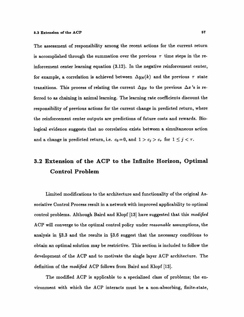
The assessment of responsibility among the recent actions for the current return

is accomplished through the summation over the previous r time steps in the re-

inforcement center learning equation (3.12). In the negative reinforcement center,

for example, a correlation is achieved between AyN(k) and the previous r state

transitions. This process of relating the current AyN to the previous As's is re-

ferred to as chaining in animal learning. The learning rate coefficients discount the

responsibility of previous actions for the current change in predicted return, where

the reinforcement center outputs are predictions of future costs and rewards. Bio-

logical evidence suggests that no correlation exists between a simultaneous action

and a change in predicted return, i.e. co = 0, and 1 > cj > c, for 1 < j < r.

3.2 Extension of the ACP to the Infinite Horizon, Optimal

Control Problem

Limited modifications to the architecture and functionality of the original As-

sociative Control Process result in a network with improved applicability to optimal

control problems. Although Baird and Klopf [13] have suggested that this modified

ACP will converge to the optimal control policy under reasonable assumptions, the

analysis in §3.3 and the results in §3.6 suggest that the necessary conditions to

obtain an optimal solution may be restrictive. This section is included to follow the

development of the ACP and to motivate the single layer ACP architecture. The

definition of the modified ACP follows from Baird and Klopf [13].

The modified ACP is applicable to a specialized class of problems; the en-

vironment with which the ACP interacts must be a non-absorbing, finite-state,

58 Chapter 8 - The Associative Control Process

finite-action, discrete-time Markov decision process. Additionally, the interface be-

tween the ACP and the environment guarantees that no acquired drive sensor will

exhibit unity output for more than a single consecutive time step. This stipulation

results in non-uniform time steps that are artificially defined as the intervals which

elapse while the dynamic state resides within a bin. 9 The learning equations of the

original ACP can be simplified by applying the fact that xz(k) E {1,0} and will

not equal unity for two or more consecutive time steps. Accordingly, (3.8) and (3.9)

yield,

r1 if z;(k)= 1

0f(A (k))= otherwise.

Therefore, a consequence of the interface between the ACP and the environment is

fS (Ax(k)) = xi(k). A similar result follows from (3.9) and (3.14).

1 if zi(k - a) = 1 and j = j,.,(k - a)f (Az(k - a))= otherwise (3.17)

The role of the reinforcement center weights becomes more well defined in the

modified ACP. The sum of the inhibitory and excitatory weights in a reinforcement

center estimate the expected discounted future reinforcement received if action j is

performed in state i, followed by optimal actions being performed in all subsequent

states. To achieve this significance, the reinforcement center output and learning

equations must be recast. The external reinforcement term does not appear in the

output equation of the reinforcement center; e.g. (3.4) becomes,

yp(k) = f (Wpim r(k)(k) + Wi j .. (k)(k)) xi(k) . (3.18)

9 Similar to §3.1, the state space is quantized into bins.

3.2 Extension of the ACP

The expression for the change in the reinforcement center output is also slightly

modified. Using the example of the negative reinforcement center, (3.13) becomes,

AyN(k) = yyN(k) - yN(k - 1) + rN(k) where 0 < 7 < 1. (3.19)

If the negative reinforcement center accurately estimates the expected discounted

future cost, AyN(k) will be zero and no weight changes will occur. Therefore, the

cost to complete the problem from time k -1 will approximately equal the cost

accrued from time k-1 to k plus the cost to complete the problem from time k. 10

yN(k - 1) = 7YN(k) + rN(k) when AyN(k) = 0 (3.20)

The value of rN(k), therefore, represents the increment in the cost functional AJ

from time k -1 to k. Recall that time steps are an artificially defined concept in

the modified ACP; the cost increment must be an assessment of the cost functional

over the real elapsed time. 11 The possibility that an action selected now does not

significantly effect the cost in the far future is described by the discount factor 7,

which also guarantees the convergence of the infinite horizon sum of discounted

future costs.

The constants in (3.7) are defined as follows: c~ = and cb=O0. Additionally,

the terms which involve the absolute values of the weights are removed from both

the motor center learning equation and the reinforcement center learning equation.

10 This statement is strictly true for 7 = 1.

"x Time is discrete in this system. Time steps will coincide with an integral number ofdiscrete time increments.

60 Chapter 3 - The Associative Control Process

Equations (3.6) and (3.12) are written as (3.21) and (3.22), respectively. With

the absence of these terms, the distinct excitatory and inhibitory weights could be

combined into a single weight, which can assume positive or negative values. This

change, however, is not made in [13].

AW =(k) I= f. (Aax(k)) [yp(k) - YN(k) - y(k)] if j = ma(k) (3.21)0 otherwise

AWgj(k) = Ayp(k) e caf, (Axij(k - a)) (3.22)a=1

The motor center learning equation (3.21) causes the motor center weights to be

adjusted so that Wg. (k) + W4j(k) will copy the corresponding sum of weights for

the reinforcement center that wins reciprocal inhibition. The saturation limits on

the motor center outputs are generalized; in contrast to (3.2), f,(x) is redefined as

fs,(x).fnf (X){1

fn,(X) = if X > P (3.23)x otherwise

Additionally, the definition of reciprocal inhibition is adjusted slightly; the non-

maximizing motor center outputs are suppressed to a minimum value -,f which is

not necessarily zero.

Although the learning process is still divided into trials, the weight increments

are incorporated into the weights at every time step, instead of after a trial has

been completed. Equations (3.10) and (3.15) are now written as (3.24) and (3.25),

respectively.

,(k) = fw+ [W (k - 1) + AW (k)] (3.24a)

W,-(k) = fw- [Wj(k - 1) + AWj(k)] (3.24b)

3.3 Motivation for the Single Layer ACP

WA(k) = fw+ [W (k - 1)+ AWA 1 (k)] (3.25a)

WFi,(k) = fw- [Wjj(k - 1) + AWYj(k)] (3.25b)

A procedural issue arises that is not encountered in the original ACP network,

where the weights are only updated at the end of a trial. The dependence of the

reinforcement center outputs on jma,(k) requires that the motor center outputs be

computed first. After learning, however, the motor center outputs and also jma,(k)

may have changed, resulting in the facilitation of a different set of reinforcement cen-

ter weights. Therefore, if weight changes are calculated such that im.,(k) changes,

these weight changes should be implemented and the learning process repeated until

jma,(k) does not further change this time step.

In general, exploration of the state-action space is necessary to assure global

convergence of the control policy to the optimal policy, and can be achieved by

occasionally randomly selecting jma(k), instead of following reciprocal inhibition.

Initiating new trials in random states also provides exploratory information.

3.3 Motivation for the Single Layer Architecture of the ACP

This section describes qualitative observations from the application of the

modified two-layer ACP to the regulation of the aeroelastic oscillator; additional

quantitative results appear in §3.6. In this environment, the modified ACP learning

system fails to converge to a useful control policy. This section explains the failure

by illustrating several characteristics of the two-layer implementation of the ACP

algorithm that are incompatible with the application to optimal control problems.

62 Chapter 3 - The Associative Control Process

The objective of a reinforcement learning controller is to construct a policy

that, when followed, maximizes the expectation of the discounted future return. For

the two-layer ACP network, the incremental return is presented as distinct cost and

reward signals, which stimulate the two reinforcement centers to learn estimates of

the expected discounted future cost and expected discounted future reward. The

optimal policy for this ACP algorithm is to select, for each state, the action with

the largest difference between estimates of expected discounted future reward and

cost. However, the two-layer ACP network performs reciprocal inhibition between

the two reinforcement centers and, therefore, selects the control action that either

maximizes the estimate of the expected discounted future reward, or minimizes the

estimate of the expected discounted future cost, depending on which reinforcement

center wins reciprocal inhibition. Consider a particular state-action pair evaluated

with both a large cost and a large reward. If the reward is slightly greater than the

cost, only the large reward will be associated with this state-action pair. Although

the true evaluation of this state-action pair is a small positive return, this action in

this state may be incorrectly selected as optimal.

The reinforcement center learning mechanism incorporates both the current

and the previous outputs of the reinforcement center. For example, the positive

reinforcement center learning equation includes the term Ayp(k), given in (3.26),

which represents the error in the estimate of the expected discounted future reward

for the previous state yp(k -1).

Ayp(k) = 7yp(k) - yp(k - 1) + rp(k) (3.26)

A reinforcement center that loses the reciprocal inhibition process will have an out-

3.3 Motivation for the Single Layer ACP

put equal to zero. Consequently, the value of Ayp(k) will not accurately represent

the error in yp(k -1) when yp(k) or yp(k -1) equals zero as a result of recipro-

cal inhibition. Therefore, Ayp(k) will be an invalid contribution to reinforcement

learning if the positive and negative reinforcement centers alternate winning re-

ciprocal inhibition. Similarly, AyN(k) may be erroneous by a parallel argument.

Moreover, the fact that learning occurs even for the reinforcement center which

loses reciprocal inhibition assures that either Ayp(k) or AyN(k) will be incorrect

on every time step that a motor center is active. If no motor center is active, no set

of weights between the acquired drive sensors and reinforcement centers are facili-

tated and both reinforcement centers will have zero outputs. Although no learning

occurs in the reinforcement centers on this time step, both Ayp and AyN will be

incorrect on the next time step that a motor center is active.

The difficulties discussed above, which arise from the presence of two com-

peting reinforcement centers, are reduced by providing a non-zero external rein-

forcement signal to only a single reinforcement center. However, the reinforcement

center which receives zero external reinforcement will occasionally win reciprocal

inhibition until it learns that zero is the correct output for every state. Using the

sum of the reinforcement center output and the external reinforcement signal as the

input to the reciprocal inhibition process may guarantee that a single reinforcement

center will always win reciprocal inhibition. 12

The optimal policy for each state is defined by the action which yields the

largest expected discounted future return. The ACP network represents this in-

12 The original ACP uses this technique in (3.4) and (3.5); the modified two-layer ACPeliminates the external reinforcement signal from the reinforcement center output in(3.18).

64 Chapter 3 - The Associative Control Process

formation in the reinforcement centers and, through learning, transfers the value

estimates to the motor centers, where an action is selected through reciprocal inhibi-

tion. The motor center learning mechanism copies either the estimate of expected

discounted future cost or the estimate of expected discounted future reward, de-

pending on which reinforcement center wins reciprocal inhibition, into the single

currently active motor center for a given state. Potentially, each time this state is

visited, a different reinforcement center will win reciprocal inhibition and a different

motor center will be active. Therefore, at a future point in time, when this state

is revisited, reciprocal inhibition between the motor center outputs may compare

estimates of expected discounted future cost with estimates of expected discounted

future reward. This situation, also generated when the two reinforcement centers

alternate winning reciprocal inhibition, invalidates the result of reciprocal inhibition

between motor centers. Therefore, the ACP algorithm to select a policy does not

guarantee that a complete set of estimates of a consistent evaluation (i.e. reward,

cost, or return) will be compared over all possible actions.

This section has introduced several fundamental limitations in the two-layer

implementation of the ACP algorithm, which restrict its applicability to optimal

control problems. By reducing the network to a single layer of learning cen-

ters, the resulting architecture does not interfere with the operation of the Drive-

Reinforcement concept to solve infinite-horizon optimization problems.

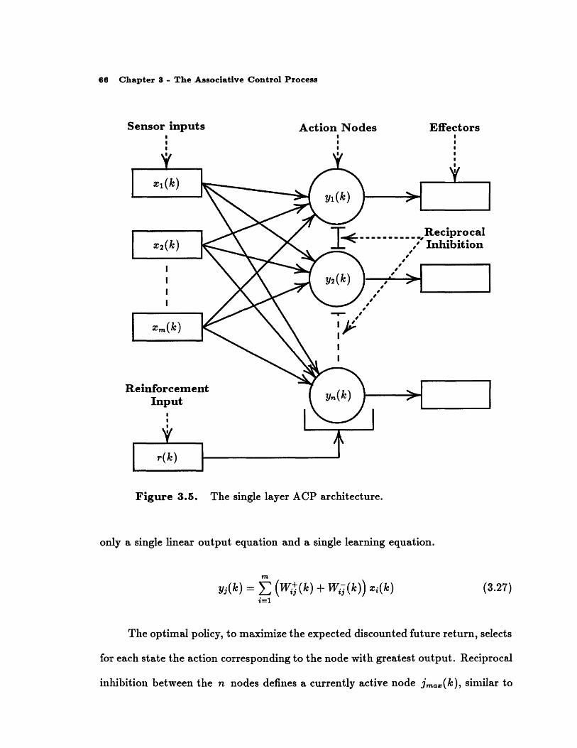
3.4 A Single Layer Formulation of the ACP

3.4 A Single Layer Formulation of the Associative Control

Process

The starting point for this research was the original Associative Control Pro-

cess. However, several elements present in the original ACP network, which are

consistent with the known physiology of biological neurons, are neither appropriate

nor necessary in a network solely intended as an optimal controller. This section

presents a single layer formulation of the modified ACP (Figure 3.5), and contains

significantly fewer adjustable parameters, fewer element types, and no nonlinearity

in the output equation. Although the physical structure of the single layer net-

work is not faithful to biological evidence, the network retains the ability to predict

classical and instrumental conditioning results [13].

The interface of the environment to the single layer network through m input

sensors is identical to the interface to the modified ACP network through the ac-

quired drive sensors. A single external reinforcement signal r(k), which assesses the

incremental return achieved by the controller's actions, replaces the distinct reward

and cost external reinforcement signals present in the two-layer network.

A node and effector pair exists for each discrete network action. 13 The output

of the jth node estimates the expected discounted future return for performing

action j in the current state and subsequently following an optimal policy. The

sum of an excitatory and an inhibitory weight encode this estimate. Constructed

from a single type of neuronal element, the single layer ACP architecture requires

'3 A node combines the functionality of the motor and reinforcement centers.

66 Chapter 3 - The Associative Control Process

Sensor inputs$

Action NodesI

Figure 3.5. The single layer ACP architecture.

only a single linear output equation and a single learning equation.

y (k) = T(W4(k) + W. -(k)) xi(k)i=1

(3.27)

The optimal policy, to maximize the expected discounted future return, selects

for each state the action corresponding to the node with greatest output. Reciprocal

inhibition between the n nodes defines a currently active node jm,,(k), similar to

Effectors

3.5 Implementation

the process between motor centers in the two-layer ACP. However, the definition of

reciprocal inhibition has been changed in the situation where multiple nodes have

equally large outputs. In this case, which represents a state with multiple equally

optimal actions, j,,,(k) will equal the node with the smallest index j. Therefore,

the controller will perform an action and will learn on every time step.

The learning equation for a node resembles that of a reinforcement center.

However, the absolute value of the connection weight at the time of the state change,

which was removed in the modified ACP, has been restored into the learning equa-

tion [13]. This term, which was originally introduced for biological reasons, is not

essential in the network and serves as a learning rate parameter. The discount fac-

tor y describes how an assessment of return in the future is less significant than

an assessment of return at the present. As before, only weights associated with a

state-action pair being active in the previous r time steps are eligible for change.

A W±(k)= [yjm.,(k)(k) - yjm..(k-1)(k - 1) + r(k)]

fC IWj±(k - a)I f. (Axij(k - a)) (3.28)a=1

0 otherwise

W,+(k) = fw+ [W+(k - 1) + AW4(k)] (3.30a)

WiJ(k) = fw- [W(k - 1) + AW(k)] (3.30b)

68 Chapter 3 - The Associative Control Process

3.5 Implementation

The modified two-layer ACP algorithm and the single layer ACP algorithm

were implemented in NetSim and evaluated as regulators of the AEO plant; fun-

damental limitations prevented a similar evaluation of the original ACP algorithm.

The experiments discussed in this section and in §3.6 were not intended to repre-

sent an exhaustive analysis of the ACP methods. For several reasons, investigations

focused more heavily on the Q learning technique, to be introduced in §4. First,

the ACP algorithms can be directly related to the Q learning algorithm. Second,

the relative functional simplicity of Q learning, which also possesses fewer free pa-

rameters, facilitated the analysis of general properties of direct learning techniques

applied to optimal control problems.

This section details the implementation of the ACP reinforcement learning

algorithms. The description of peripheral features that are common to both the

ACP and Q learning environments will not be repeated in §4.5.

The requirement that the learning algorithm's input space consist of a finite

set of disjoint states necessitated a BOXES [8] type algorithm to quantize the con-

tinuous dynamic state information that was generated by the simulation of the AEO

equations of motion. 14 As a result, the input space was divided into 200 discrete

states. The 20 angular boundaries occurred at 180 intervals, starting at 00; the 9

boundaries in magnitude occurred at 1.15, 1.0, 0.85, 0.7, 0.55, 0.4, 0.3, 0.2, and 0.1

14 The terms bins and discrete states are interpreted synonymously. The aeroelasticoscillator has two state variables: position and velocity. The measurement of thesevariables in the space of continuous real numbers will be referred to as the dynamicstate or continuous state.

3.5 Implementation

nondimensional units; the outer annulus of bins did not have a maximum limit on

the magnitude of the state vectors that it contained.

The artificial definition of time steps as the non-uniform intervals between

entering and leaving bins eliminates the significance of r as the longest interstimulus

interval over which delay conditioning is effective.

The ACP learning control system was limited to a finite number of discrete

outputs: +0.5 and -0.5 nondimensional force units.

The learning algorithm operated through a hierarchical process of trials and

experiments. Each experiment consisted of numerous trials and began with the ini-

tialization of weights and counters. Each trial began with the random initialization

of the state variables and ran for a specified length of time. 15 In the two-layer archi-

tecture, the motor center and reinforcement center weights were randomly initialized

using uniform distributions between {-1.0, -a} and {l, 1.0}. In the single layer

architecture, all excitatory weights were initialized within a small uniform random

deviation of 1.0, and all inhibitory weights were initialized within a small uniform

random deviation of -a. The impetus for this scheme was to originate weights suf-

ficiently large such that learning with non-positive reinforcement (i.e. zero reward

and non-negative cost) would only decrease the weights.

The learning system operates in discrete time. At every time step, the dy-

namic state transitions to a new value either in the same bin or in a new bin and

the system evaluates the current assessment of either cost and reward or reinforce-

ment. For each discrete time step that the state remains in a bin, the reinforcement

15 Initial states (position and velocity) were uniformly distributed between -1.2 and+1.2 nondimensional units.

70 Chapter 3 - The Associative Control Process

Table 3.1. ACP parameters.

Name Symbol Value

Discount Factor 7 0.95

Threshold 0 0.0

Minimum Bound on IWI a 0.1

Maximum Motor Center Output 13 1.0

Maximum Interstimulus Interval 7 5

accumulates as the sum of the current reinforcement and the accretion of previous

reinforcements discounted by 7. The arrows in Figure 3.6 with arrowheads lying in

Bin 1 represent the discrete time intervals that contribute reinforcement to learning

in Bin 1. Learning for Bin 1 occurs at ts where the total reinforcement equals the

sum of rs and 7 times the total reinforcement at t4.

Figure 3.6. A state transition and reinforcement accumulation car-toon.

For the two-layer ACP, the reward presented to the positive reinforcement

center was zero, while the cost presented to the negative reinforcement center was

a quadratic evaluation of the state error. In the single layer learning architecture,

Bin 1 t2 Bin 2

t3

3.6 Results

the quadratic expression for the reinforcement signal r, for a single discrete time

interval, was the negative of the product of the square of the magnitude of the

state vector, at the final time for that interval, and the length of that time interval.

The quadratic expression for cost in the two-layer ACP was -r. The magnitude of

the control expenditure was omitted from the reinforcement function because the

contribution was constant for the two-action control laws.

r= -(2 - t3 ) [X(t 2)2 ] (3.31)

3.6 Results

Figure 3.7 illustrates a typical segment of a trial, prior to learning, in which

an ACP learning system regulated the AEO plant; the state trajectory wandered

clockwise around the phase plane, suggesting the existence of two stable limit cycles.

The modified two-layer ACP system failed to learn a control law which drove

the state from an arbitrary initial condition to the origin. Instead, the learned

control law produced trajectories with unacceptable behavior near the origin (Figure

3.8). The terminal condition for the AEO state controlled by an optimal regulator

with a finite number of discrete control levels, is a limit cycle. However, the two-

layer ACP failed to converge to the optimal control policy. Although the absence of

a set of learning parameters for which the algorithm would converge to an optimal

solution cannot be easily demonstrated, §3.3 clearly identifies several undesirable

properties of the algorithm.

72 Chapter 3 - The Associative Control Process

1.0

0 .5 .............. .......... -4 -------- - ------- ------ ------------- ---- -- ----- ------------

05. .. ..................... ..........

-1.0'-2.0 -1.5 -1.0 -0.5 0.0 0.5 1.0 1.5

Position

Figure 3.7. A characteristic AEO state trajectory achieved by areinforcement learning algorithm prior to learning.

The single layer architecture of the ACP learned the optimal control law, which

successfully regulated the AEO state variables near zero from any initial condition

within the region of training, {-1.2,1.2}. The performance of the control policy

was limited by the coarseness of the bins and the proximity of bin boundaries to

features of the nonlinear dynamics. The restricted choice of control actions also

bounds the achievable performance, contributing to the rough trajectory in Figure

3.9. I I II (

i '-0 5 ............... ........ ......." ' II ,I r tI I-1. ' r

-2. -1. -1. -0. 0. . ..I~Position

Figure 3.7 A hrceitcAE tt rjcor civdbrifocmn lernn alorth prio tolrig

The ~ ( sigelyra ietre of he AC erndteoimlctrllwwhh

succesfull reulte the AEO stt vaibe erzr rm ntaodtowithir th eino rii, {-.2 1.} Th efrac ftecnrlplc

was liie by th oreeso h isadtepoiiyo In onais

feaure of theI nolna dyais Th resrite chieo otoltoss

bons h hevbe efomnccotibtn to the rog tajetr n Fiur

3.9. , I I

1.0

0.8---

0.6 -

0.4---

0.2----

0.0

-0.2

-0.4 --1.0 1.0-0.5 0.0 0.5

Position

Figure 3.8. The AEO state trajectory achieved by the modifiedtwo-layer ACP after learning.

.0 -0.5 0.0Position

0.5 1.0

Figure 3.9. The AEO state trajectory achieved by the single layerACP after learning.

3.6 Results

U)

2o0U

1.0

0.8

0.6

0.4

0.2

0.0

-0.2

-0.4

-0.6-1

. - -- -e -- -- --°---- ----------- o--------- ----- o ---- ---- ------- - -- ----- ----

I ,i........................... .......................... ............................-1

...........................,.........................., .............. ---- ------------------

.......................... ........................... ---- ................... .. .......................

.- 8

-

74

Chapter 4

Policy and Value Iteration

The notation and concepts presented in §4.1 through §4.4 follow directly from

Watkins' thesis [16] and [17]. §4.5 and §4.6 present results of applying Q learning

to the AEO. §4.7 explores a continuous version of Q learning.

4.1 Terminology

4.1.1 Total Discounted Future Return

A discrete-time system that performs an action ak in a state Xk, at time k,

receives a performance evaluation rk associated with the transition to the state Xk+1

at time k + 1; the evaluation rk is referred to as the return at time k. 1 The total

future return after time k, which equals the sum of the returns assessed between

time k and the completion of the problem, may be unbounded for an infinite

1 Watkins defines return as the total discounted future reward; this paper equates theterms return and reward.

76 Chapter 4 - Policy and Value Iteration

horizon problem. However, the return received in the distant future is frequently

less important, at the present time, than contemporary evaluations. Therefore,

the total discounted future return, defined in (4.1) and guaranteed to be finite, is

proposed.

00

7E "rk+n = k + 7rk+1 + 72rk+2 + ... + "rk+ +... (4.1)n=O

The discount factor, 0 < 7 < 1, determines the present value of future returns.

4.1.2 The Markov Decision Process

A non-absorbing, finite-state, finite-action, discrete time Markov decision pro-

cess is described by a bounded set of states S, a countable set of actions for each

state A(x) where x e S, a transition function T, and an evaluation mechanism R.

At time k, the state is designated by a random variable Xk and the true value xk.

The transition function defines Xk+ = T(Xk,ak) where ak E A(lk); the new state

must not equal the previous state with probability equal to unity. At time k, the

return is denoted by a random variable Rk = R(xk, ak) and the actual evaluation

T k. The expectation of the return is written RI . The Markov property implies that

the transition and evaluation functions depend on the current state and current

action, and do not depend on previous states, actions, or evaluations.

4.1.3 Value Function

In a Markov decision process, the expectation of the total discounted future

return depends only on the current state and the stationary policy. A convenient

notation for the probability that performing action a in state x will leave the

4.1 Terminology

system in state y is P,,(a). The random variable representing the future state

Xk+n achieved by starting in the state Xk at time k and following policy f for n

time steps is written as X(k, f,n).

X(k, f, 0) = Xk (4.2a)

X(Xk,f,1) = Xk+1 = T(xk,f(Xk)) (4.2b)

If policy f is followed for n time steps from state Xk at time k, the return realized

for applying f(zk+n) in state zk+n is expressed as R(xk, f, n).

R(k, f, O) = R(Zk, f(zk)) = Rk (4.3a)

R(Xk, f, n) = R(Xk+n, f(Xk+n)) = Rk+n (4.3b)

The expected total discounted future return subsequent to the state z, applying

the invariant policy f, is the value function Vf(z).

Vf(z) = R(z, f,O) + yR(x, f, 1) + ... + nR(., f,n) +... (4.4a)

= R(x, f, 0) + 7Vf (X(x, f, 1)) (4.4b)

= R(x, f, 0) + -E P,,(f(x)) V(y) (4.4c)

In (4.4c), y is the subset of S that is reachable from x in a single time step.

4.1.4 Action Value

The action-value Qf(z, a) is the expectation of the total discounted future

return for starting in state x, performing action a, and subsequently following

78 Chapter 4 - Policy and Value Iteration

policy f. Watkins refers to action-values as Q values. A Q value represents the

same information as the sum of an excitatory weight and an inhibitory weight in

Drive-Reinforcement learning, which is used in the single layer ACP.

Qf(z, a) = R(x, a) + y Py(a)Vf(y) (4.5)

The expression for an action-value (4.5) indicates that the value function for policy

f must be completely known prior to computing the action-values.

Similarly, Qf(x, g) is the expected total discounted future return for starting

in x, performing action g(x) according to policy g, and subsequently following

policy f.

4.2 Policy Iteration

The Policy Improvement Theorem [16] states that a policy g is uniformly

better than or equivalent to a policy f if and only if,

Qf(x,g) > V(x) for all x E S. (4.6)

This theorem and the definition of action-values imply that for a policy g which

satisfies (4.6), V,(x) > Vf(x) for all x E S. The Policy Improvement Algorithm

selects an improved policy g according to the rule: g(x) = a G A(x) such that

a is the argument that maximizes Qf(x,a). However, to determine the action-

values Qf(x, a) for f, the entire value function Vf(x) must first be calculated. In

4.3 Value Iteration

the context of a finite-state, finite-action Markov process, policy improvement will

terminate after applying the algorithm a finite number of times; the policy g will

converge to an optimal policy.

The Optimality Theorem [16] describes a policy f* which cannot be improved

using the policy improvement algorithm. The associated value function Vf.(x) and

action-values Qf.(, a) satisfy (4.7) and (4.8) for all x E S.

Vf.(x) = max Qf.(x,a) (4.7)aEA(,)

f*(x) = a such that Qf.(z,a)= Vf.(x) (4.8)

The optimal value function and action-values are unique; the optimal policy is

unique except in states for which several actions yield equal and maximizing action-

values.

4.3 Value Iteration

The value iteration [16] procedure calculates an optimal policy by choosing for

each state the action which effects a transition to the new state that possesses the

maximum evaluation; the optimal value function determines the evaluation of each

state that succeeds the current state. The expected total discounted future return

for a finite horizon process which consists of n transitions and a subsequent final

return, to evaluate the terminal state, is represented as V . The value function,

80 Chapter 4 - Policy and Value Iteration

which corresponds to the infinite horizon problem, is approximated by repeatedly

applying rule (4.9) to an initial estimate VO.

Vn(X A() ( (4.9)V"(m) = ax [R(x, a) + -rE Py(a)Vn-(Y)] (4.9)

Value iteration guarantees that the limit in (4.10) approaches zero uniformly over

all states. Therefore, V n converges to the optimal value function and the optimal

policy can be derived directly from V'7.

lirm I V - V.I = 0 (4.10)

Although this procedure is computationally simplest if all states are systematically

updated so that V n is completely determined from Vn- before Vn +1 is calculated

for any state, Watkins has demonstrated that the value iteration method will still

converge if the values of individual states are updated in an arbitrary order, provided

that all states are updated sufficiently frequently.

4.4 Q Learning

Unfortunately, neither the optimal policy nor optimal value function can be

initially known in a control problem. Therefore, the learning process involves si-

multaneous, incremental improvements in both the policy function and the value

function. Action-values Qf,(Zk, ak) for each state-action pair at time k contain

4.5 Implementation

both policy and value information; the policy and value functions at time k are

defined in (4.11) and (4.12) in terms of Q values.

fk() = a such that Qk(,a)=V2(x) (4.11)

VkQ(x) = max [Qk(x, a)] (4.12)

The superscript Q denotes the derivation of the policy and the value function from

the set of action-values Qfk (xk, ak). Single step Q learning adjusts the action-values

according to (4.13).

Qk+1(x, ak) = (1 - )Qk(xk, ak) + a(rk + 7Vk(Xk+l)) (4.13)

The positive learning rate constant a is less than unity. Only the action-value

of the state-action pair (xk, ak) is altered at time k; to guarantee convergence of

the value function to the optimal, each action must be repeatedly performed in

each state. As a form of dynamic programming, Q learning may be described as

incremental Monte-Carlo value iteration.

4.5 Implementation

This section formalizes the implementation of the Q learning algorithm as a

regulator for the aeroelastic oscillator plant. The environment external to the Q

learning process was similar to that used for the ACP experiments in §3.5 and §3.6.

82 Chapter 4 - Policy and Value Iteration

However, the quantization of the state space was altered. The boundaries of the

260 bins that covered the state space were defined by magnitudes M and angles

A; the outer annulus of bins did not have a maximum magnitude.

M = {0.0, 0.05, 0.1, 0.15, 0.2, 0.25, 0.3, 0.35, 0.4, 0.5, 0.6,

0.7, 0.85, 1.0}

A = {00, 180, 360, 540, 720, 900, 1080, 1260, 1440, 1620, 1800, 1980,

2160, 2340, 2520, 2700, 2880, 3060, 3240, 3420}

The bins were labeled with integer numbers from 0 to 259, starting with the bins

in the outer ring, within a ring increasing in index with increasing angle from 00,

and continuing to the next inner ring of bins.

For each state-action pair, the Q learning algorithm stores a real number that

represents the Q value. At the start of a new NetSim experiment, all Q values were

initialized to zero.

The two parameters which appear in (4.13) were: y = 0.95 and a = 0.5. In

this context, a is a learning rate parameter; in the ACP description, a was the

minimum bound on the absolute value of the weights. The return rk was given in

(3.31) as the negative of the product of the squared magnitude of the state vector

and the length of the time interval.

4.6 Results

The results of two experiments, conducted in the NetSim [11] environment,

characterize the performance of the Q learning algorithm. The two experiments

1.00

0.85

0.70

0.60

0.50

0.40

0.30

0.25

0.20

0.15

0.10

0.05

0.00

differ in the set of allowable control actions.

Ezperiment 1:

Experiment 2:

Uk E {0.5, -0.5}

Uk e {0.5, 0.33, 0.167, 0.0, -0.167, -0.33, -0.5}

The learned optimal policy for Ezperiment 1 appears in Figures 4.1a and 4.1b.

The control law applied a +0.5 force whenever the state resided in a bin containing

a + and applied -0.5 whenever the state was in an empty bin. The general form of

this control policy resembles the non-optimal bang-bang law that was derived from

4.6 Results

+ + + + + + + + + + +

+ + + + + + + +

+ + + + + + + +

+ + + + + + + + + + +

+ + + + + + + + + +

+ + + + + + + + ++ +S+ + + + + + + ++ + + + + + + + + +

+ + + + + + + + +++ + + + + + ++ +

+ + + + + + + + + +

0 342 324 306 288 270 252 234 216 198 180 162 144 126 108 90 72 54 36 18 0

Angular Divisions (degrees)

Figure 4.1a. A Cartesian representation of the two-action optimalcontrol policy.

108 0 72 0

1.00

.85

.70. . . . ... ..

+ .60 +

.50

.40

.30

.25

.20

++.10

+ + + +" .. + +. ' . • . .

++ +:+ + + + ±44.+ + .. -

+ + 4"

+ + ... +.. .. +. ++ ++:•~ ~ ~ ~+' .+-+ -.. -. +. i .:.:-+....+..-

• + • .. .+ - .. + : + . . . .+.'+ +

S. . . • .++. . ±-" +

2160 .+

+234 o0

252 0

54 o0

360

180

+ .:+

.. +.+ :

+

342 o0

+

t + .*. - - ++ + ... '4- . . +

+ + .. ±-1

: ±

±

.7

+324 0

306 o0

2880

270 o0

Figure 4.lb. A polar representation of the two-action optimal con-trol policy.

a LQR solution in §2.4.3. Figure 2.9 demonstrated that for the non-optimal bang-

bang control policy, the state trajectory slowly approached the origin along a linear

84 Chapter 4 - Policy and Value Iteration

90 o0

126 o0

144 o

+

1620

180 .

198 o0

+

+

.. :.. . . ..

4.6 Results

!!

.............. Force = -0.5-2.5 ---------- --------- ------ -------1.0 ......-1.50 50 00 150............... 200 250

-2.0 ........ .................... * ........ Force = 0.5 ...........

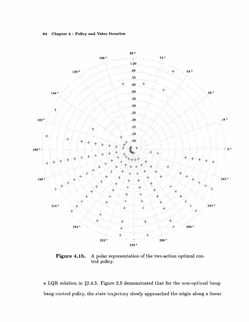
value) for each state-action pair.= -0.5-2.5 .......................................................................... .....................-3.0 '_'0 50 100 150 200 250Box Number

Figure 4.2. Experiment 1: Expected discounted future return (Qvalue) for each state-action pair.

switching curve. To avoid the high cost of this behavior, the optimal two-action

solution will not contain a linear switching curve. A positive force must be applied

in some states where the bang-bang rule (§2.4.3) dictated a negative force and a

negative force must be applied in some bins below the linear switching curve. The

trajectories that result from the control policies constructed in Experiments 1 and

2 avoid the problem of slow convergence along a single switching curve. Although

some regions of the control policy appear to be arbitrary, there exists a structure.

For two bins bounded by the same magnitudes and separated by 1800, the optimal

actions will typically be opposite. For example, the three + bins bounded by 0.6,

0.7, 54' , and 108' are reflections of the blank bins bounded by 0.6, 0.7, 2340, and

86 Chapter 4 - Policy and Value Iteration

0.0

-0.5 -------------- --.. .................... .....................

1......... ................--.............

I I

O Force = 0.5-1.5 - . .-- ....... .......... Force = 0.333 --------

S- - Force = 0.167Force = 0.0

-2.0 ............ ..................... ........ .......Force = -0.167Force = -0.33

-2.5 .-- -- .............------------------------------.....................--- ----- Force = -0.5 ........

-3.00 50 100 150 200 250

Box Number

Figure 4.3. Experiment 2: Expected discounted future return (Qvalue) for each state-action pair.

2880. The 15 pairs of bins which violate this pattern lie primarily near the linear

switching curve (§2.4.3).

Figures 4.2 and 4.3 compare the expected discounted future returns for all

state-action pairs in Experiments 1 and 2, respectively. The expected discounted

future return was negative for all state-action pairs because only negative return

(i.e. cost) was assessed. Moreover, the Q values for bins nearer the origin were

greater than the Q values for outlying bins. The fact that a non-optimal action

performed in a single bin does not significantly affect the total cost for a trajectory,

when optimal actions are followed in all other bins (in this problem), explains the

similarity between most Q values associated with different actions and the same

4.6 Results

state. Additionally, the Q values varied almost periodically as a function of the

bin number; the largest variance existed for the bins farthest from the origin. All

trajectories tended to approach the origin along the same paths through the second

and fourth quadrants (Figures 4.4, 4.6, 4.8, and 4.10). Therefore, if an initial

condition was such that the limited control authority could not move the state onto

the nearest path toward the origin, then the trajectory circled halfway around the

state space to the next path toward the origin. This characteristic was a property

of the AEO nonlinear dynamics, and accounted for the large differences in Q values

for neighboring bins. In Experiment 1, there existed bins for which the choice of the

initial control action determined whether this circling was necessary. For these bins,

the expected discounted future returns for the two actions differed substantially.

The control law constructed in Experiment 2 was expected to outperform

the control law constructed in Experiment 1 (i.e. for each bin, the maximum Q

value from Figure 4.3 would exceed the maximum Q value from Figure 4.2). For

the data presented, this expectation is true for 60% of the bins. The bins that

violate this prediction are entirely located in the regions of the state space that the

state enters least frequently. Experiment 2, with a greater number of state-action

pairs, requires substantially more training than Experiment 1. The fact that for

certain bins, the maximum Q value from Experiment 1 exceeds that for Experiment

2 signals insufficient learning in those bins for Experiment 2.

No explicit search mechanism was employed during learning. Moreover, the

dynamics tended to force all trajectories onto the same paths, so that many bins

were seldom entered. Therefore, to assure that a globally optimal policy was at-

tained, sufficient trials were required so that the random selection of the initial

88 Chapter 4 - Policy and Value Iteration

1.0

0.8 ------------------------ ------------------------------------

0.6 --------------------------------------------------- --------------- - --------------------------

-0.2 ----------.------------------------------------------ + .--------- - - ---------------------

0.8-----0.2 ------------ --------------------------- ....... ...- -

0.2 ------------ -------- ---------------........- --------- -Figure 4.4. Experiment 1: Contrajectory, ,o = f -1.0, 0.5}.

..... ... ............ .......

S0.0 -------- -I0.4 ----.0 ------------- - - - --

o o o - o o o o o - o o - o o o - o o o o o o - o - - o - - - - - ' - - - - - - - o o o - " o o o

. . .

-0.6 --------

-0.8

Time

Figure 4.5. Experiment 1: Control history, _o = {-1.0,0.5}.0 4 ............ --~- ~-- ----ri02 '

0.2 .......... ..

0 2 4 6 8 10--~~~~~~~~~~~~Time

Fiue .. ze imet1 oto istrZ_ -. ,.

4.6 Results 89

0.60.4 --------------------. --------------------- ...................... -------------------- -------------------0............. ......................--..---------------------------------- ------------------0.2 ----------------

0.0 ----

0 -0.2 ---------------- --- -------------------- --------------------- --------------------- -- ------------------0. ------------------- --..--------------- ----- --------------- ----- - ------------------.. .................

I ! I i

-1.0 -0.5 0.0 0.5 1.0 1.5

Position

Figure 4.6. Experiment 1: State trajectory, o = {1.0,0.5}.

0.6 ..................... -------------------- -------------------- --------------------- ---------------------

0.4 ------ ------- ------- --

0.-------- ------ ............ .. --..0.2 --------- -o 0.-2 --- ----- -- -- ------------------------ -

-0.2 -----

-0.4 -----

-0.6 -.. --....----- - ------------------- ----------------------------- ---- ----------------

-0.80 2 4 6 8 10

Time

Figure 4.7. Experiment 1: Control history, _o = {1.0,0.5}.

90 Chapter 4 - Policy and Value Iteration

Z%

1.0

0.8

0.6

0.4

0.2

0.0

-0.2 ----------

-04 -----------0.4 ..

-0.6-1.0

Figure 4.8.

0.8

0.6

0.4

0.2

0.0

-0.2

-0.4

-0.6

-0.8

-0.5 0.0 0.5

Position

Experiment 2: State trajectory, .o = {-1.0,0.5}.

Time

Experiment 2: Control history, o = {-1.0,0.5}.

1.0

* I I I. I IIII

.... .....I'. -. -

III I

I I i I

I I I I------------- i------------ --------------

i I IiI I II I I I

i I I

Figure 4.9.

I

4.6 Results

0.6

0.4

0.2

0.0

8 -0.2

-0.4

-0.6

-0.8

-1.0-1.0 -0.5 0.0 0.5 1.0

Position

Figure 4.10.

0.8

0.6

0.4

0.2

0.0

-0.2

-0.4

-0.6

-0.8

Experiment 2: State trajectory, o = {1.0,0.5}.

Time

Ezperiment 2: Control history, -o = {1.0, 0.5}.

I I I

............. ...--- --. ..... - ---------------- 4--------------- ---------------: I !

............--- - ------------ ---- ------------- - -------------- -- -------, , I'Ie o 8

.................. .................... --.........------ ---- ------.-------I I I .e iI~ i

I ! I !I II II I

Ir Iii

e i i i

o o I oI

, , , rI I II !,- - - -- - - - -- -- - - - - - - - - - - - - - - - - - --- - - - --- - - - - - - - - - - - - - - -- - - - -- - - - -

- - - -- - - - - -- - - - - - - - - -- - - - - - - - - - - - -

1.5

--.-.-.... ------------------------------ ----------

.- .-------- -------------- --

i I I iI S

- - -- - - -- 4 - - - - 4 -S.- ....................- -.----- -- - - --

I

Figure 4.11.

92 Chapter 4 - Policy and Value Iteration

state provided sufficient experience about performing every action in every bin.

Over 2000 trials were performed in each experiment to train the learning system.

If the learning rate had been a focus of the research, an explicit search procedure

could have been employed. Additionally, in some experiments, the Q values did not

converge to a steady state. Some of the bins were excessively large such that the

optimal actions (in a continuous sense) associated with extreme points within the

bin were quite different. Therefore, the Q values for such a bin, and subsequently

the optimal policy, would vary as long as training continued.

All Q learning experiments learned a control policy that successfully regulated

the aeroelastic oscillator. The state trajectories and control histories of the AEO,

with initial conditions {-1.0,0.5} and {1.0,0.5}, which resulted from the control

laws learned in Experiments 1 and 2, appear in Figures 4.4 through 4.11. The lim-

itation of the control to discrete levels, and the associated sharp control switching,

resulted in rough state trajectories as well as limit cycles around the origin. The

results illustrate the importance of a smooth control law; a continuous control law

(LQR) was discussed in §2.4.2 and a characteristic state trajectory appeared in Fig-

ure 2.5. The absence of actuator dynamics and a penalty on the magnitude of the

control allow the application of larger values of control to maximize reinforcement.

Therefore, Experiment 2 seldom selected a smaller or zero control force, even for

bins near the origin. In Experiment 1 the magnitude of the control was constant.

4.7 Continuous Q Learning

4.7 Continuous Q Learning

The algorithm described in §4.4 operates with both a finite set of states and

discrete control actions. The optimal control a* maximizes Q(x, a*) for the current

state z. To identify the optimal control for a specific state, therefore, requires the

comparison of Q(x, a) for each discrete action a E A(x).2 However, quantization

of the input and output spaces is seldom practical or acceptable

-........ 4--------------4 -- -------... . ..... --------10I I

I I .......... IiiI I

I e II I I i

-----------

Control

Figure 4.12. A continuous Q function for an arbitrary state x.I I ei ~Iii

i i IeeI l

e l e

lI e l eI Il e. | . . . . . .. . .

I I I. I

e i l I

I~ I Ie

i e e

l I e

i I I I

Ii r i i e

I e v ( eII e I l

I I I I I

eiur e.2 e eotnosQfnto o nabtaysae2

A potential new algorithm, related to the Q learning process of §4.4 might se-

2 A finite number of Q values exist and, therefore, the maximum Q value is easilyobtained.

94 Chapter 4 - Policy and Value Iteration

lect, for each discrete state, the optimal control action from a bounded continuum

and employ a continuous Q function that maps the control levels into evaluations

of the expected discounted future return (Figure 4.12). However, to identify the

optimal control for a state requires the maximization of a potentially multi-modal

bounded function; this extremization procedure is problematic relative to the max-

imization of discrete Q values. The maximization of a multi-modal function at each

stage in discrete time is itself a complicated optimization problem and, although not

intractable, makes any continuous Q learning procedure impractical for real-time,

on-line applications. This Q learning algorithm directly extends to incorporate

several control variables; the optimal controls for a state are the arguments that

maximize the multidimensional Q function.

The Q learning concept may be further generalized to employ continuous in-

puts and continuous outputs. The algorithm maps expectations of discounted future

returns as a smooth function of the state and control variables. The current state

will define a hyperplane through this Q function that resembles Figure 4.12 for a

single control variable. Again, a maximization of a potentially multi-modal func-

tion is required to compute each control. Although the continuous nature of the

state inputs does not operationally affect the identification of an optimal control,

the mapping and learning mechanisms must incorporate the local generalization of

information with respect to state, a phenomenon which does not occur for discrete

state bins. A continuous Q function could be represented by any function approxi-

mation scheme, such as the spatially localized connectionist network introduced in

§6.

Baird [42] addressed the difficulty of determining the global maximum of a

4.7 Continuous Q Learning 95

multi-modal function. Millington [41] proposed a direct learning control method

that used a spatially localized connectionist / Analog Learning Element. The

learning system defined, as a distributed function of state, a continuous probability

density function for control selection.

96

Chapter 5

Temporal Difference Methods

Temporal difference (TD) methods comprise a class of incremental learning

procedures that predict future system behavior as a function of current observa-

tions. The earliest temporal difference algorithm appeared in Samuel's checker-

playing program [18].1 Manifestations of the TD algorithm also exist in Holland's

bucket brigade [19], Sutton's Adaptive Heuristic Critic [5,20], and Klopf's Drive-

Reinforcement learning [12]. This chapter summarizes Sutton's unification of these

algorithms into a general temporal difference theory [15] and then analyzes the simi-

larities and distinctions between the Adaptive Heuristic Critic, Drive-Reinforcement

learning, and Q learning.

1 The phrase temporal difference was proposed by Sutton in 1988 [15].

97

98 Chapter 5 - Temporal Difference Methods

5.1 TD( A) Learning Procedures

Most problems to which learning methods are applicable can be formulated

as a prediction problem, where future system behavior must be estimated from

transient sequences of available sensor outputs. Conventional supervised learning

prediction methods associate an observation and a final outcome pair; after train-

ing, the learning system will predict the final outcome that corresponds to an input.

In contrast, temporal difference methods examine temporally successive predictions

of the final result to derive a similar mapping from the observations to the final

outcome. Sutton demonstrates that TD methods possess two benefits relative to

supervised learning prediction methods [15]. Supervised learning techniques must

wait until the final outcome has been observed before performing learning calcula-

tions and, therefore, to correlate each observation with the final outcome requires

storage of the sequence of observations that preceded the final result. In contrast,

the TD approach avoids this storage requirement, incrementally learning as each

new prediction and observation are made. This fact, and the associated temporal

distribution of required calculations, make the TD algorithm amenable to running

on-line with the physical plant. Through more efficient use of experience, TD al-

gorithms converge more rapidly and to more accurate predictions. Although any

learning method should converge to an equivalent evaluation with infinite expe-

rience, TD methods are guaranteed to perform better than supervised learning

techniques after limited experience with a Markov decision process.

Temporal difference and conventional supervised learning are indistinguishable

for single step prediction problems where the accuracy of a prediction is revealed

5.1 TD( A) Learning Procedures

immediately. In a multi-step prediction problem, partial information pertinent to

the precision of a prediction is incrementally disclosed through temporally suc-

cessive observations. This second situation is more prevalent in optimal control

problems. Multi-stage problems consist of several temporally sequential observa-

tions {zx, z2 , ... , ,m} followed by a final result z. At each discrete time t, the

learning system generates a prediction Pt of the final output, typically dependent

on the current values of a weight set w. The learning mechanism is expressed as a

rule for adjusting the weights.

Typically, supervised learning techniques employ a generalization of the

Widrow-Hoff rule [21] to derive weight updates. 2

Awt = a(z - Pt)AP (5.1)

In contrast to (5.1), TD methods are sensitive to changes in successive predictions

rather than the error between a prediction and the final outcome. Sutton has

demonstrated that for a multi-step prediction problem, a TD(1) algorithm produces

the same total weight changes for any observation-outcome sequence as the Widrow-

Hoff procedure. The TD(1) algorithm (5.2) alters prior predictions to an equal

degree.

Awt = a(Pt+1 - P) 1 A.Pt (5.2)k=1

The temporal difference method generalizes from TD(1) to an algorithm that adjusts

prior predictions in proportion to a factor that equals unity for the current time and

2 The Widrow-Hoff rule, also known as the delta rule, requires that Pt be a linearfunction of w and xt so that A,Pt = zt.

100 Chapter 5 - Temporal Difference Methods

decreases exponentially with increasing elapsed time. This algorithm is referred to

as TD( A) and (5.3) defines the learning process, where Pm+1 is identically z.

t

Aw = a(Pt+ - P,) E At -kAP (5.3)k=1

0 < A < 1 (5.4)

An advantage of this exponential weighting is the resulting simplicity of determining

future values of the summation term in (5.3).

t+1 t

S(t + 1)= At+1-k wpk = AWPt+1 + t+1- k (5.5)k=1 k=1

= A.p,+ + A At-kA"Pk = AWPt+ 1 + AS(t)k=1

In the limiting case where A = 0, the learning process determines the weight in-

crement entirely by the resulting effect on the most recent prediction. This TD(0)

algorithm (5.6) resembles (5.1) if the final outcome z is replaced by the subsequent

prediction.

awt = a(P+ - P)AWP (5.6)

5.2 An Extension of TD(A)

The TD family of learning procedures directly generalizes to accomplish the

prediction of a discounted, cumulative result, such as the expected discounted future

5.3 A Comparison of Reinforcement Learning Algorithms

cost associated with an infinite horizon optimal control problem. In conformance

with Sutton's notation, ct denotes the external evaluation of the cost incurred

during the time interval from t -1 to t. The prediction Pt, which is the output of

the TD learning system, estimates the expected discounted future cost.

00oo

Pt 7nCt+1+n (5.7)n=0

The discount parameter y specifies the time horizon with which the prediction

is concerned. The recursive nature of the expression for an accurate prediction

becomes apparent by rewriting (5.7).

oo00 00

Pt - = Ct + E 7 yct+ = Ct + 7t y _ct+n+l = Ct + 7Pt (5.8)n=1 n=O

Therefore, the error in a prediction, (ct + 7Pt) - Pt-i, serves as the impetus for

learning in (5.9).

Lwt = a(ct + P, - Pt-1) E At-kAwPk (5.9)k=1

5.3 A Comparison of Reinforcement Learning Algorithms

The modified TD( A) rule (5.9) is referred to as the Adaptive Heuristic Critic

(AHC) and learns to predict the summation of the discounted future values of the

signal ct. With slightly different learning equations, both Q learning and Drive-

Reinforcement (DR) learning accomplish a similar objective. This section compares

the form and function of these three direct learning algorithms.

101

102 Chapter 5 - Temporal Difference Methods

The single step Q learning algorithm (5.10) defines a change in a Q value,

which represents a prediction of expected discounted future cost, directly, rather

than through adjustments to a set of weights that define the Q value.

Qt+l(zt, at) = (1 - o)Qt(zt, a) + a(ct + Vt (t+l)) (5.10)

Although the form of the learning equation appears different than that of the AHC

or DR learning, the functionality is similar. The improved Q value Qt+1(xt, at)

equals a linear combination of the initial Q value Qt(xt, at) and the sum of the

cost for the current stage ct and the discounted prediction of the subsequent dis-

counted future cost yVQ (xt+i). A similar linear combination to perform incremental

improvements is achieved in both the AHC and Drive-Reinforcement learning by

calculating weight changes with respect to the current weights.

Both the Drive-Reinforcement (DR) and the Adaptive Heuristic Critic learn-

ing mechanisms calculate weight changes that are proportional to the prediction

error APt.

APt = ct + 7 Pt - Pt-1 (5.11)

The DR learning rule is rewritten in (5.12) to conform to the current notation.

Awt = AP ck fs (At-k) (5.12)k=l

In the DR and AHC algorithms, a non-zero prediction error causes the weights to

be adjusted so that Pt-1 would have been closer to ct + /Pt. The constant of

5.3 A Comparison of Reinforcement Learning Algorithms

proportionality between the weight change and the prediction error differs between

DR learning and the AHC.

The Drive-Reinforcement weight changes are defined by (5.12). The limits

oni the summation over previous stages in time and the binary facilitation function

f, prescribe modifications to a finite number of previous predictions. An array

of constants, Ck, encode a discount that determines the contribution of previous

actions to the current prediction error. In contrast, the summation term in the AHC

learning equation (5.9) allows all previous predictions to be adjusted in response

to a current prediction error. The extent to which an old prediction is modified

decreases exponentially with the elapsed time since that prediction. In the AHC

algorithm, the sensitivity of the prior prediction to changes in the weights, APk,

scales the weight adjustment.

Similar to the AHC and DR learning, an incremental change in a Q value is

proportional to the prediction error.

AQt(xt, at) = Qt+i(xt, at) - Qt(xt, at) = a (ct - Qt(xt, at) + TVt(xt+1 )) (5.13)

The expression for the prediction error in (5.13) appears different from (5.11) and

warrants some explanation. V(x+ 1l), which represents maxa [Qt(xt+l, at+l)], de-

notes the optimal prediction of discounted future cost and, therefore, is functionally

equivalent to Pt in (5.11). Moreover, the entire time basis for Q learning is shifted

forward one stage with respect to the AHC or DR learning rules. As a result, Qt

operates similar to Pt-1 in (5.11) and the symbol ct performs the same function in

(5.11) and (5.13), although the cost is measured over a different period of time in the

Q learning rule than in the AHC or DR learning rules (5.9) and (5.12), respectively.

103

104 Chapter 5 - Temporal Difference Methods

To summarize the comparison of direct learning algorithms, each of the three

temporal difference techniques will learn a value function for the expected dis-

counted future cost. More generally, any direct learning algorithm will maintain

and incrementally improve both policy and value function information. Further-

more, although the forms of the learning equations differ slightly, each method

attempts to reduce the prediction error APt.

Although the functionality of direct learning algorithms may be similar, the

structure will vary. For example, Q learning distinguishes the optimal action by

maximizing over the set of Q values. The Associative Control Process determines

the optimal action through the biologically motivated reciprocal inhibition proce-

dure. Furthermore, whereas Q values may equal any real number, the outputs of

ACP learning centers must be non-negative, acknowledging the inability of neurons

to realize negative frequencies of firing.

Chapter 6

Indirect Learning Optimal Control

Each control law derived in this chapter attempts to optimally track a refer-

ence trajectory that is generated by a linear, time-invariant reference model (6.1);

optimization is performed with respect to quadratic cost functionals over finite time

horizons. The notation in this chapter uses subscripts to indicate the stage in dis-

crete time and superscripts to distinguish the plant and reference model.

S= (rx + r'rk (6.la)

y = CO4 (6.lb)

Yk+I = Cr'rxr + crrrrk (6.lc)

Yk+2 = CP r + crt rrk + Cr t rk+l (6.1d)

Although a few subsequent values of the command input after rk may be charac-

terized at time k, the future input sequence will be largely unknown. To apply

105

106 Chapter 6 - Indirect Learning Optimal Control

infinite horizon, linear quadratic (LQ) control techniques to the tracking problem

requires a description of the future command inputs. Furthermore, in a multi-

objective mission, such as aircraft flight involving several different flight conditions,

the existence of future maneuvers should negligibly influence the optimization of

performance during the current operation. Finally, optimizations over unnecessar-

ily long time frames may require prohibitively long computations. Therefore, finite

horizon LQ control directly addresses relevant control problems.

6.1 Single-Stage Quadratic Optimization

The control objective is to minimize the quadratic cost functional Jk which

penalizes the current control expenditure and the output error ek+1, given by the

difference between the reference output and the system output at time k+1. The

weighting matrices R and Q are symmetric and positive definite.

2 [ kT+1lQek+ 1 + alRuk]

ek+1 = Yk+1 - Yk+l

(6.2)

(6.3)

A single first-order necessary condition defines the condition for a control uk to

minimize the cost functional Jk [22,23].

- 0 (6.4a)(uk

6.1 Single-Stage Quadratic Optimization

uek+ Qek+l + Ruk = 0 (6.4b)

6.1.1 Linear Compensation

Assuming a minimum-phase plant, the linear compensator is the solution to

the problem of optimal tracking, with respect to the cost functional (6.2), of the

reference system (6.1) with a linear, time-invariant system (6.5). Applied to a

nonlinear system, this control law serves as a baseline with which to compare a

single-stage, indirect learning control law. The fact that indirect learning control

is a model based technique distinguishes the approach from direct learning control

algorithms.

Xk+1 = (Xk + ruk (6.5a)

Yk = CXk (6.5b)

yk+i = Cixk + Cruk (6.5c)

That the partial derivative of ek+l with respect to uk is independent of uk implies

that (6.4b) is linear in the optimal control. Therefore, (6.4b) may be written as an

exact analytic expression for the optimal control [24].

= -CT (6.6)8Uk

k = [(cr)TQCr + R] -' (c)TQ [CG'4 + CT'rTk - Ck] (6.7)

107

108 Chapter 6 - Indirect Learning Optimal Control

The sufficient condition for this control to be a minimizing solution, that ' 2j

is non-negative, is satisfied for physical systems.

= -(CF)TQek+l + Ruk = 0 (6.8)8uk

a_= (Cr)TQ(CF) + R > 0 (6.9)

6.1.2 Learning Control

In contrast to the single-stage linear compensator, the single-stage, indirect

learning controller is the solution to the problem of optimal tracking of the refer-

ence system (6.1) by a nonlinear, time-invariant system (6.10), with respect to the

cost functional (6.2). Again, the zero dynamics of the plant must be stable. The

expression for the discrete time state propagation (6.10a) includes the a priori linear

terms from (6.5) as well as two nonlinear terms: fk(xk,Uk) represents the initially

unmodeled dynamics that have been learned by the system, and I~k(xk) represents

any state dependent dynamics not captured by either the a priori description or the

learning augmentation. The assumption of an absence of time varying disturbances

and noise from the real system implies that all dynamics are spatially dependent

and will be represented in the model. The system outputs are a known linear com-

bination of the states. The notation explicitly shows the time dependence of fk

and Tk, which change as learning progresses; fk will acquire more of the subtleties

in the dynamics and, consequently, "k will approach zero.

Xk+1 = 4Xk + rUk + fk(Xk, Uk) + ' k(Xk) (6.10a)

6.1 Single-Stage Quadratic Optimization

Yk = C k (6.10b)

Yk+1 = CkXk + cruk + Cfik(Xk,7k) + C]k(Xk) (6.10c)

In this formulation, the first-order necessary condition (6.4) for a control Uk

to be optimal with respect to (6.2) cannot be directly solved for Uk because of

the presence of the term fk(Xk, Uk) which may be nonlinear in uk. The Newton-

Raphson iterative technique [25] addresses this nonlinear programming problem by

linearizing fk(xk,ulk) with respect to u at uk-1. 2 is the Jacobian matrix of fk

with respect to u, evaluated at {Xk, Uk-1}. Using this approximation for fk(xk, uk),

yk+1 assumes a form linear in Uk and (6.4) may be written as an analytic expression

for Uk in terms of known quantities.

fkk(XkUik) F fk(XkUk-1) + (Uk - Uk-1) (6.11)Wk,uk-.1

Ofyk+, C9z k + Cruk + Cfk(k, uk-1) + C (Uk - Uk-1) + CXk(xk) (6.12)

9uXkUk-1

Bek+1 -SCr-C (6.13)OUk -9U & hkuh--

The solution (6.14) is the first Newton-Raphson estimate for the optimal con-

trols; a pseudo-inverse may be used in (6.14) if the full matrix inversion does not

exist. Subsequent estimates ui may be derived by linearizing (6.10) about u.-1

However, the estimate obtained in the first iteration is often sufficiently accurate

because the initial linearization is about uk-1 and the admissible change in control

Auk = Uk - Uk-1 will be limited by actuator rate limits and a sufficiently small

discrete time interval [25,26].

109

110 Chapter 6 - Indirect Learning Optimal Control

The form of the learning augmented control law closely resembles the linear

control law (6.7). In (6.14) CF is modified by ' which describes the variation in

control effectiveness that was unmodeled in the linear system. The final three terms

of (6.14) are not present in (6.7) and enter from the nonlinear terms in (6.10).

U= CF+C QjCF+CL R -

CF + C af Q C'['x + C 'rk - Cxk

Of ( (6.14- Cf(xk, Uk-1) + C k-1 - kk) 61)

A simple adaptive estimate for the unmodeled dynamics at time k is generated

by solving (6.10) at the previous time index for 'k-1(Xk-1) and assuming 'k(Xk) 1

Tk-(Xk-1). This adaptive technique is susceptible to noise and disturbances present

in the real system [27].

''k(Xk) = Xk - 44k-1 - ruk-l - fk(Xk-1,k-1) (6.15)

6.1.3 Penalizing Control Rate

A parallel set of arguments may be used to derive a control law that is opti-

mal with respect to a cost functional that also penalizes changes in control. The

A uTSAuk component in (6.16) discourages large control rates that may not be

achievable, as a result of physical limitations of the actuators. The control law

6.2 Two-Step Quadratic Optimization

(6.18) resembles (6.14) with the addition of two terms involving S, which is sym-

metric and positive definite.

S[eT Qek+ + uRuk + ATSAuk] (6.16)

AUk = uk - Uk-1 (6.17)

Uk= C[(r+ CO T Q C+C-) +R+S 1

Cv + TQ (CrrX + CTrk - k

- Cfk(xk, k-1) Cuk-1 - C Xk)) + Suk-1 (6.18)

6.2 Two-Step Quadratic Optimization

This section parallels the discussion of §6.1 to derive the control laws that are

optimal with respect to a two time step, quadratic cost functional (6.19); a few new

issues arise. The expression for the reference output two time steps into the future

(6.1d) involves a future value of the command input rk+1 . This derivation assumes

that rk+l e Trk

1= +[T Q le ke+ + T Q2ek+2 + U'R 0oU T+ U Ruk+1 (6.19)S= k+- k+2 k + uk+l

111

112 Chapter 6 - Indirect Learning Optimal Control

Two necessary conditions are required to define a control which is optimal with

respect to (6.19). Each of the weighting matrices in (6.19) is symmetric and positive

definite.

0Jk9 = 0

OUk,(6.20a)

(ek+1 T k+9U&k+l Qek+l +

+ (OUk +T Q2 ek+2 + RoUk = 0

OJk= 0

8Uk+l

8Uk+2) Q 2 ek+2 + Rluk+l = 0t9Uk+1/

6.2.1 Linear Compensation

The output of the linear system (6.5) two time steps into the future is easily

determined because the dynamics are assumed to be entirely known.

Yk+2 = Cmxk + C~ruk + Cruk+l (6.22)

ek+2 = Yk+2 - Yk+2 (6.23)

The simultaneous solution of (6.20b) and (6.21b) yields a solution for Uk; an ex-

pression for Uk+l, calculated at time k, is also available. However, to parallel the

learning control process, this control will be recalculated at the next time step. To

e 1k+ek+lkOUk / le~ (6.20b)

(6.21a)

(6.21b)

6.2 Two-Step Quadratic Optimization

illustrate the similarity of the linear and learning control laws, as well as to express

the laws in a compact form, several substitutions are defined.

A = CF (6.24a)

B = C(F (6.24b)

A = ATQ 2A + R 1 (6.25a)

T = BTQ 2 A (6.25b)

0 = ATQ 1 (6.25c)

= (BT - TA-1AT)Q 2 (6.25d)

uk = [ATQ 1 A + BTQ 2B + Ro - TA-1TT] 1

[(0 C'' + 2 C''#7 ) r

+ (o CT'r + E (C''r'r + C'r')) k

- (o Ct + E Ccbl) x] (6.26)

6.2.2 Learning Control

For the nonlinear system, the output yk+2 (6.27a) must be approximated by

known quantities that are linear in Uk and uk+1 . First, the nonlinear terms in

(6.27a) are evaluated at the current time k rather than at k +1 and an approxi-

mation 4k+l is derived for the next state. Additionally, the learned dynamics are

118

114 Chapter 6 - Indirect Learning Optimal Control

estimated by linearizing fk(xk+l,uk+1) about the point {Xk,Uk-1}.

k+1 = Xk + rUk + fk(Xk, Uk-) +

affk(Xk+1 Ek+1 0 fk(Xk, k-l)+

Xk k1

Uk k- Uk 1 ) + k(k)

(6.27a)

(6.27b)

(6.28)X

Xkstk-1

Of(Uk+l- Uk-+ '+1 - Xk) (6.29)

XkZUkl1

ofYk+2 C "- -k+ + CFUkl + Cfk(XkUk-l) C (Uk+ 1 - Uk- 1 )

k,Uk-- 1

+C (k+l - Xk) + Cl'k(X k+1)

XkUk-1

(6.30)

Using this approximation for yk+2, the simultaneous solution of (6.20b) and

(6.21b) yields an expression for uk in terms of (6.25) and (6.31). The variables A

and B include both the linear components of the a priori model as well as learned

state dependent corrections. 2f is a correction to the constant F matrix and 9f

is a correction to the constant ( matrix.

OfA = CF + Cu

Of Of OfB = C(P + C4Of + C r + Cu Oau 49X Ou ax

(6.31a)

(6.31b)

Although the simultaneous solution of the first-order necessary conditions also yields

an expression for Uk+l at k, uk is calculated on every time step. This control

Yk+2 = CPXk+l

SC &xk+l

+ CrUk+1 + Cfk+1(kl , Uk+l) + C'lk+l(Xk+1)

+ CrUk+1 + Cfk(Xk+1, k+l)+ C'lk( k+1)

6.3 Implementation and Results

law resembles the form of (6.26) and introduces several terms associated with the

nonlinear dynamics.

Uk = [ATQ 1A + BTQ 2 B + Ro - TA-xTT]-

(0 C?' + EO'' ") X,'

+ (o CT'r + E (C'9'r' + C'r)) rk

f f Of

+ C + C + C 1k-1ou Ou 9u ex ou))

-(oc+ (c+ E + C - k(Xk

- Ck(-k+1)] (6.32)

6.2.3 Multi-stage Quadratic Optimization

The arguments presented in §6.1 and thus far in §6.2 may be generalized to

derive a control law which is optimal with respect to a cost functional (6.33) that

looks n time steps into the future. The solution of this problem, however, will

require assumptions about the propagation of the command input r for n future

time steps. Additionally, the algebra required to write an explicit expression for uk

becomes involved and the necessary linearizations become less accurate.

1k = [e iQiek+ T+i- , k+i- AuT+i1SiA +i_]i (6.33)

115

116 Chapter 6 - Indirect Learning Optimal Control

6.3 Implementation and Results

6.3.1 Reference Model

The reference model, which generates trajectories that the plant states at-

tempt to follow, exhibits a substantial influence on the closed-loop system perfor-

mance. While a reference model that does not satisfy performance specifications will

yield an unacceptable closed-loop system, a reference model that demands unreal-

istic (i.e. unachievable) state trajectories may introduce instability through control

saturation. Therefore, the reference model must be selected to yield satisfactory

performance given the limitations of the dynamics [28].

The reference model was selected to be the closed-loop system that resulted

from applying the optimal control from a linear quadratic design, to the aeroelastic

oscillator dynamics linearized at the origin [29]. The discrete time representation of

the reference model as well as the AEO linear dynamics are presented for At = 0.1.

Q=[ 1 (6.34a)

R = 1.0 * 10-7 (6.34b)

C = C [ 0.11] (6.35)

[ 0.994798 0.1060701 (6.36a)-0.106070 1.122083

r=[0.005202] (6.36b)

6.3 Implementation and Results

[ 0.905124 0.000286-0.905124 -0.000286

F = [0.905124] (6.37b)

Design of an optimal control law might be accomplished with a learning system

that incrementally increases closed-loop performance requirements, by adjusting the

reference trajectory in regions of the state space where the current control law can

achieve near perfect tracking. This is a topic for future research.

6.3.2 Function Approximation

The discussion of direct learning optimal control (§3 - §5) focused on learn-

ing system architectures and algorithms which, themselves, operate as controllers.

The discussion of indirect learning optimal control is primarily concerned with the

manner in which experiential information about unmodeled dynamics may be in-

corporated into optimal control laws. The method by which a supervised learning

system approximates the initially unmodeled dynamics is a separate issue which

has received much investigation [21,30,31,32].

After a brief summary, this thesis abstracts the technique for realizing the

nonlinear mapping f(x, u) into a black box which provides the desired information:

fk(xk, Uk-l), 2 Jkk,uk1, and fk(Xk-1, Uk-l)*

A spatially localized connectionist network is used to represent the mapping

from the space of states and control to the initially unmodeled dynamics. The linear-

Gaussian network achieves spatial locality by coupling a local basis function with

an influence function [4,28]. The influence function, which determines the region in

117

118 Chapter 6 - Indirect Learning Optimal Control

the input space of applicability of the associated basis function, is a hyper-Gaussian;

the basis function is a hyperplane.

The contribution of a basis function to the network output equals the product

of the basis function and the influence function, evaluated at the current input,

where the influence function is normalized so that the sum of all the influence

functions at the current input is unity [28]. The control law provides to the network

an estimate of the model errors, Xk - xzk-1 - FUk-1. The supervised learning

procedure follows an incremental gradient descent algorithm in the space of the

network errors by adjusting the parameters that describe the slopes and offsets of

the basis functions.

In terms of equations and for arbitrary input and output dimensions, Y(x)

is the network output evaluated at the current input x. The network consists of n

nodes (i.e. basis function and influence function pairs).

Y(x) = Z Li()r(x) (6.38a)i=1

Li(x) is the evaluation of the ith basis function at the current input. Wi is a

weight matrix that defines the slopes of the hyperplane and bi is a bias vector. x0o

defines the center of the influence function.

L i (x) = Wi(x - xo) + bi (6.38b)

Fi(x) is the ith normalized influence function and is not related to the discrete time

B matrix. Gi(z) is the ith influence function evaluated at x, where the diagonal

6.3 Implementation and Results

matrix Di represents the spatial decays of the Gaussians.

Ii (X) - Gi(x)

Gi(x) = exp -(X - X0)TD?(x - XO)]

The learning network had three inputs (position, velocity, and control) and

two outputs (unmodeled position and velocity dynamics). In addition, the partial

derivatives of the system outputs with respect to the inputs were available.

1.0

0.5

-0.0

-0.5

-1.0-1.0 -0.5 0.0 0.5

Velocity

1.0

Figure 6.1. The initially unmodeled velocity dynamics g(x 2) as afunction of velocity z 2 .

(6.38c)

(6.38d)

119

120 Chapter 6 - Indirect Learning Optimal Control

The AEO dynamics are repeated in (6.39). The learning system must syn-

thesize on-line the initial model uncertainty, which consists of the nonlinear term

g(X 2) in the velocity dynamics.

]_ 0 ] [x] + [0 + 0(6.39a)1 nAjU - 2P x2 1 g(22)

g(X 2 ) = 1 n 3 (1000x2) 3 + (1000x 2 )5 A (1000x 2 (6.39b)g( 1000 U U U(10)7 (.9)

The manner in which the position and control enter the dynamics is linear and

perfectly modeled. Therefore, the function f will be independent of the position

and control (Figure 6.1). Additional model errors may be introduced to the a priori

model by altering the coefficients that describe how the state and control enter the

linear dynamics. The learning system will approximate all model uncertainty.

Although the magnitude of the control had been limited in the direct learning

control results, where the reinforcement signal was only a function of the state

error, limitation of the control magnitude was not necessary for indirect learning

controllers because control directly entered the cost functional.

6.3.3 Single-Stage Quadratic Optimization Results

For the minimization of the weighted sum of the squares of the current control

and the succeeding output error, the performance of the learning enhanced control

law (6.14) was compared to the associated linear control law (6.7), in the context

of the aeroelastic oscillator. Results appear in Figures 6.2 through 6.9. The control

and reference model were updated at 10 Hz; the AEO simulation was integrated

using a fourth-order Runge-Kutta algorithm with a step size of 0.005.

6.3 Implementation and Results

1.0

0.8 ---- .........

Reference Position0.6 " ------.----- --------. Reference Velocity

Learning PositionLearning Velocity

0.4 -..-.. .....-----i------ ------- --------- Linear Position

........... Linear Velocity

0.2 ------ .............. ------------. .---------- ------------------ 4

model as well as the AEO controlled by the linear andlearning control laws, for the command r = 1 and theinitial condition i = o, 0}.

Figure 6.2 illustrates the reference model position and velocity time histories

as well as two sets of state time histories for the AEO controlled by the linear and

learning control laws. The presence of unmodeled nonlinear dynamics prevented

the linear control law from closely tracking the reference position. In contrast,

the learning system closely followed the reference, after sufficient training. Both

control laws maintained the velocity near the reference. Although the full learning

control law (6.14) was implemented to produce these results, knowledge of the form

of the AEO nonlinearities could have been used to eliminate the terms containing

!. Figure 6.3 represents the errors between the AEO states and the referenceOu"

121

122 Chapter 6 - Indirect Learning Optimal Control

0.20

0.15

0.10

0.05

0.0

-0.05

-0.10

Time

Figure 6.3.

0.1-

-0.1 - -

-0.2 -

-0.3 -

-0.4 -.

The state errors for the AEOand learning control laws.

controlled by the linear

0 2 4 6 8Time

10

Figure 6.4. The network outputs that were used to compute Ukfor the learning control law.

2 4 6 8 10 12 14

6.3 Implementation and Results

model, for both control law designs. In a separate experiment that introduced

model uncertainty in the linear dynamics, the linear control law (6.7) failed to

track a command step input with zero steady-state error. The learning control law

results looked similar to Figure 6.2.

The specifics of the incremental function approximation were not a focus of

this indirect learning control research. The learning process involved numerous

trials (more than 1000) from random initial states within the range {-1.0, 1.0};

the commanded position was also selected randomly between the same limits. The

allocation of network resources (i.e. adjustable parameters) and the selection of

learning rates involved heuristics. Moreover, the learning performance depended

strongly on these decisions. Automation of the network design process would have

greatly facilitated this research.

The learning control law requires the values of the network outputs at the

current state and the previous control, as well as the partial derivative of the network

outputs with respect to the control, at the current state and the previous control.

Additionally, the adaptive term 'k(Xk) requires the values of the network outputs

at the previous state and the previous control. The network outputs, which appear

in Figure 6.4, change most rapidly when the velocity is not near zero, i.e. at the

beginning of a trial. Some rapid changes in the network outputs resulted from

learning errors where f did not accurately approximate the nonlinear dynamics.

For the learning control law, the control as well as the terms of (6.14) that

comprise the control appear in Figure 6.5. The control for the linear control law

and the individual terms of (6.7) appear in Figure 6.6.

After substantial training, some errors remained in the network's approxima-

128

124 Chapter

10

8

6

4

2

0

-2

-4

-6

6 - Indirect Learning Optimal Control

Uk

S---- -------- ---

. \

iiX- , ter -- fk( k,Uk - ) term

: r term ukl term- --

x term ----- k(k) term

0 2 4 6 8 10

Figure 6.5. The control uking control law

10

5

0

-5

-10

Time

and the constituent terms of the learn-(6.14).

0 2 4 6 8Time

Figure 6.6. The control Uk and the constituent terms of the linearcontrol law (6.7).

6.3 Implementation and Results

0.0

-0.05 - ---------

-0.10---------------------

Position Term-0.15 ...................................... ... ................----------- Velocity Term

-0.20 ---- -- ----------- -------------------- -------------------- -------------------- ---------------------

-0.25-0 1 2 3 4 5

Time

Figure 6.7. The estimated errors in the approximation of the ini-tially unmodeled dynamics fk(xk, k-1).

tion of the nonlinear dynamics. These errors are most noticeable in the estimation

of the velocity dynamics at velocities not near zero. Figure 6.8 illustrates the initial

model errors not represented by the function f; the adaptive term will reduce the

effect of these remaining model errors. Experiments demonstrated that the system

performed nearly as well when the adaptive contribution was removed from the con-

trol. A controller that augmented the linear law with only the adaptive correction

was not evaluated.

Figure 6.8 shows the results of control laws (6.14) and (6.7) regulating the AEO

from o = {-1.0, 0.5}. The control magnitude was limited at 0.5 so that the results

may be compared more easily to the benchmarks and the direct learning control

results. Time is not explicitly shown in Figure 6.8; the state trajectory produced by

125

126 Chapter 6 - Indirect Learning Optimal Control

0U>

1.0

0.8

0.6

0.4

0.2

0.0

-0.2

-0 A

-1.0 -0.5 0.0

Position

Figure 6.8. AEO Regulation from 0 = {-1.0,saturation at ±0.5.

0.5} with control

2 4 6 8Time

10 12 14

Control history associated with Figure 6.8.

. . . . . . .. .. .. .. . . . . -------------------------- ------------------------- --------------------------

................. .................... .- ----------------! e............................. . .........................-- ------------------------

.......... ............. ...... ........................... Linear aI a

0.5 1.0

0.6

0.4

0.2

0.0

-0.2

-0.4

-0.60

Figure 6.9.

6.3 Implementation and Results

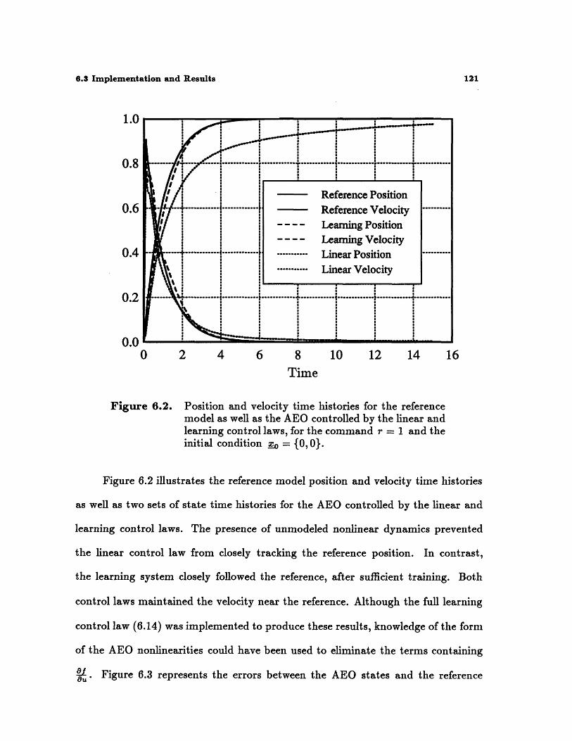
the learning controller approached the origin much more quickly than the trajectory

produced by the linear controller. The control objective remains to track a reference

trajectory and, therefore, subtly differs from the goal of LQR (Figure 2.5). Recall

that this reference model does not necessarily maximize system performance. Figure

6.9 shows the force histories which yielded the trajectories in Figure 6.8. The rapid

switching in the learning control force results from learning errors and the sensitivity

of the control law to the approximated Jacobian of fk(xk, k-1).

This indirect learning control technique was capable of learning, and therefore

reducing the effect of, model uncertainty (linear and nonlinear). Therefore, the

indirect learning controller derived from a linear model with model errors performed

similar to Figure 6.8 and outperformed the LQR solution which was derived from an

inaccurate linear model (Figure 2.7). The indirect learning controller with limited

control authority produced state trajectories similar to the results of the direct

learning control experiments.

127

128

Chapter 7

Summary

The aeroelastic oscillator demonstrated interesting nonlinear dynamics and

served as an acceptable context in which to evaluate the capability of several direct

and indirect learning controllers.

The ACP network was introduced to illustrate the biological origin of rein-

forcement learning techniques and to provide a foundation from which to develop

the modified two-layer and single layer ACP architectures. The modified two-layer

ACP introduced refinements that increased the architecture's applicability to the

infinite horizon optimal control problem. However, results demonstrated that, for

the defined plant and environment, this algorithm failed to synthesize an optimal

control policy. Finally, the single layer ACP, which functionally resembled Q learn-

ing, successfully constructed an optimal control policy that regulated the aeroelastic

oscillator.

Q learning approaches the direct learning paradigm from the mathematical

theory of value iteration rather than from behavioral science. With sufficient train-

129

180 Chapter 7 - Summary

ing, the Q learning algorithm converged to a set of Q values that accurately de-

scribed the expected discounted future return for each state-action pair. The opti-

mal policy that was defined by these Q values successfully regulated the aeroelastic

oscillator plant. The results of the direct learning algorithms (e.g. the ACP deriva-

tives and Q learning) demonstrated the limitations of optimal control laws that

are restricted to discrete controls and a quantized input space. The concept of ex-

tending Q learning to accommodate continuous inputs and controls was considered.

However, the necessary maximization at each time step of a continuous, poten-

tially multi-modal Q function may render impractical an on-line implementation of

a continuous Q learning algorithm.

The optimal control laws for single-stage and two-step finite time horizon,

quadratic cost functionals were derived for linear and nonlinear system models. The

results of applying these control laws to cause the AEO to optimally track a linear

reference model demonstrated that indirect learning control systems, which incor-

porate information about the unmodeled dynamics that is incrementally learned,

outperform fixed parameter, linear control laws. Additionally, operating with con-

tinuous inputs and outputs, indirect learning control methods provide better perfor-

mance than the direct learning methods previously mentioned. A spatially localized

connectionist network was employed to construct the approximation of the initially

unmodeled dynamics that is required for indirect learning control.

7.1 Conclusions

This thesis has collected several direct learning optimal control algorithms and

7.1 Conclusions

has also introduced a class of indirect learning optimal control laws. In the process

of investigating direct learning optimal controllers, the commonality between an

algorithm originating in behavioral science and another founded in mathematical

optimization help unify the concept of direct learning optimal control. More gen-

erally, this thesis has "drawn arrows" to illustrate how a variety of learning control

concepts are related. Several learning systems were applied as controllers for the

aeroelastic oscillator.

7.1.1 Direct / Indirect Framework

As a means of classifying approaches to learning optimal control laws, a di-

rect/indirect framework was introduced. Both direct and indirect classes of learning

controllers were shown to be capable of synthesizing optimal control laws, within

the restrictions of the particular method being used. Direct learning control implies

the feedback loop that motivates the learning process is closed around system per-

formance. This approach is largely limited to discrete inputs and outputs. Indirect

learning control denotes a class of incremental control law synthesis methods for

which the learning loop is closed around the system model. The indirect learning

control laws derived in §6 are not capable of yielding stable closed-loop systems for

non-minimum phase plants.

As a consequence of closing the learning loop around system performance,

direct learning control procedures acquire information about control saturation.

Indirect learning control methods will learn the unmodeled dynamics as a function

of the applied control, but will not "see" control saturation which occurs external

to the control system.

181

132 Chapter 7 - Summary

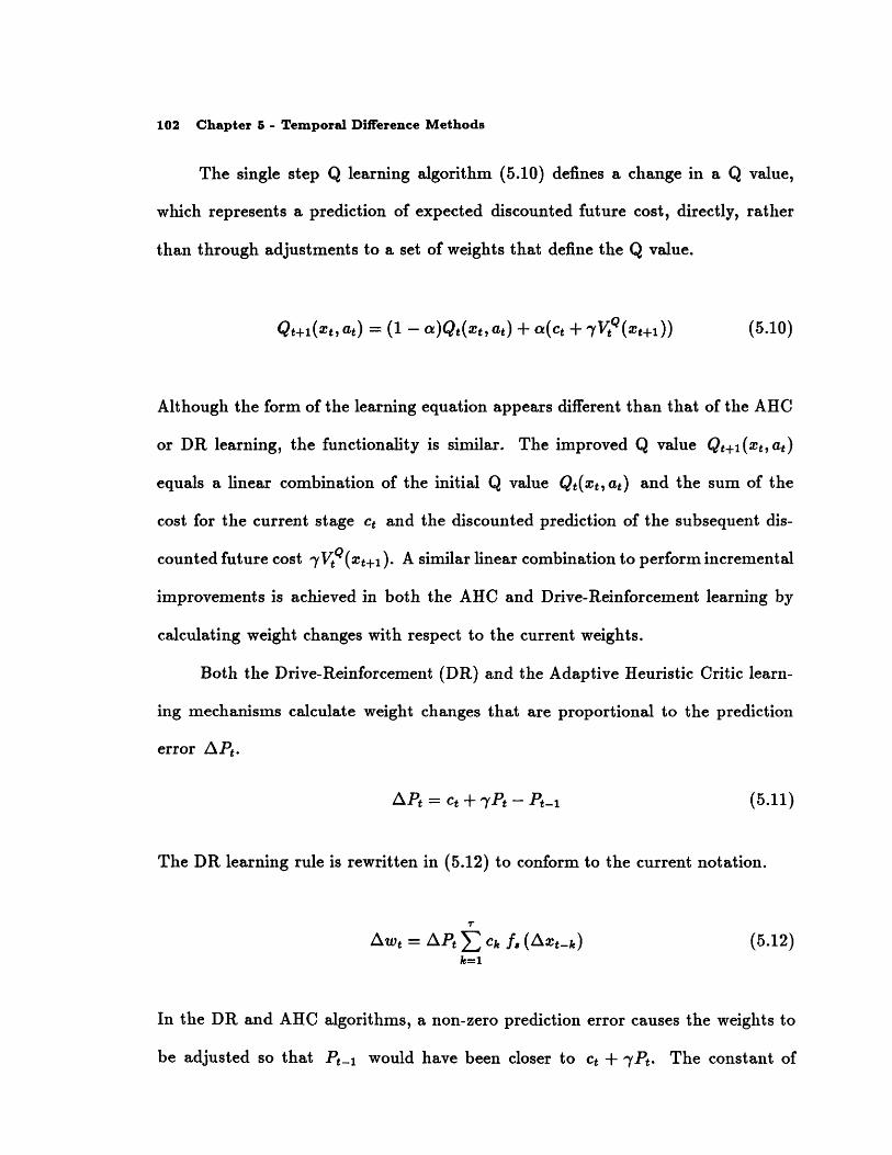
7.1.2 Comparison of Reinforcement Learning Algorithms

The learning rules for the Adaptive Heuristic Critic (a modified TD( A) pro-

cedure), Q learning, and Drive-Reinforcement learning (the procedure used in the

ACP reinforcement centers) were compared. Each learning system was shown to

predict an expected discounted future reinforcement. Moreover, each learning rule

was shown to adjust the previous predictions in proportion to a prediction error that

was the difference between the current reinforcement and the difference between the

previous expected discounted future reinforcement and the discounted current ex-

pected discounted future reinforcement. The constants of proportionality describe

the reduced importance of events that are separated by longer time intervals.

7.1.3 Limitations of Two-layer ACP Architectures

The limitations of the two-layer ACP architectures arise primarily from the

simultaneous operation of two opposing reinforcement centers. The distinct posi-

tive and negative reinforcement centers, which are present in the two-layer ACP,

incrementally improve estimates of the expected discounted future reward and cost,

respectively. The optimal policy is to select, for each state, the action that maxi-

mizes the difference between the expected discounted future reward and cost. How-

ever, the two-layer ACP network performs reciprocal inhibition between the two

reinforcement centers. Therefore, the information passed to the motor centers ef-

fects the selection of a control action that either maximizes the estimate of expected

discounted future reward, or minimizes the estimate of expected discounted future

cost. In general, a two-layer ACP architecture will not learn the optimal policy.

7.2 Recommendations for Future Research

7.1.4 Discussion of Differential Dynamic Programming

For several reasons, differential dynamic programming (DDP) is an inappro-

priate approach for solving the problem described in §1.1. First, the DDP algorithm

yields a control policy only in the vicinity of the nominally optimal trajectory. Ex-

tension of the technique to construct a control law that is valid throughout the state

space is tractable only for linear systems and quadratic cost functionals. Second,

the DDP algorithm explicitly requires, as does dynamic programming, an accurate

model of the plant dynamics. Therefore, for plants with initially unknown dynamics,

a system identification procedure must be included. The coordination of the DDP

algorithm with a learning systems that incrementally improves the system model

would constitute an indirect learning optimal controller. Third, since the quadratic

approximations are valid only in the vicinity of the nominal state and control trajec-

tories, the DDP algorithm may not extend to stochastic control problems for which

the process noise is significant. Fourth, similar to Newton's nonlinear programming

method, the original DDP algorithm will converge to a globally optimal solution

only if the initial state trajectory is sufficiently close to the optimal state trajectory.

7.2 Recommendations for Future Research

Several aspects of this research warrant additional thought. The extension

of direct learning methods to continuous inputs and continuous outputs might be

an ambitious endeavor. Millington [41] addressed this issue by using a spatially

localized connectionist / Analog Learning Element that defined, as a distributed

133

134 Chapter 7 - Summary

function of state, a continuous probability density function for control selection.

The learning procedure increased the probability of selecting a control that yielded,

with a high probability, a large positive reinforcement. The difficulty of generalizing

the Q learning algorithm to continuous inputs and outputs has previously been

discussed.

The focus of indirect learning control research should be towards methods of

incremental function approximation. The accuracy of the learned Jacobian of the

unmodeled dynamics critically impacts the performance of indirect learning optimal

control laws. The selection of network parameters (e.g. learning rates, the number

of nodes, and the influence function centers and spatial decay rates) determines how

successfully the network will map the initially unmodeled dynamics. The procedure

that was used for the selection of parameters was primarily heuristic. Automation of

this procedure could improve the learning performance and facilitate the control law

design process. Additionally, indirect learning optimal control methods should be

applied to problems with a higher dimension. The closed-loop system performance

as well as the difficulty of the control law design process should be compared with

a gain-scheduled linear approach to control law design.

Appendix A

Differential Dynamic Programming

A.1 Classical Dynamic Programming

Differential dynamic programming (DDP) shares many features with the clas-

sical dynamic programming (DP). For this reason, and because dynamic program-

ming is a more recognized algorithm, this chapter begins with a summary of the

dynamic programming algorithm. R. E. Bellman introduced the classical dynamic

programming technique, in 1957, as a method to determine the control function that

minimizes a performance criterion [33]. Dynamic programming, therefore, serves as

an alternative to the calculus of variations, and the associated two-point boundary

value problems, for determining optimal controls.

Starting from the set of state and time pairs which satisfy the terminal con-

ditions, the dynamic programming algorithm progresses backward in discrete time.

To accomplish the necessary minimizations, dynamic programming requires a quan-

tization of both the state and control spaces. At each discrete state, for every stage

135

136 Appendix A - Differential Dynamic Programming

in time, the optimal action is the action which yields the minimum cost to com-

plete the problem. Employing the principle of optimality, this completion cost from

a given discrete state, for a particular choice of action, equals the sum of the cost

associated with performing that action and the minimum cost to complete the prob-

lem from the resulting state [23]. J*(I_) equals the minimum cost to complete a

problem from state x and discrete time t, g(x, I, t) is the incremental cost func-

tion, where u is the control vector, and T(x, u, t) is the state transition function.

Further, define a mapping from the state to the optimal controls, S(_; t) = u(t)

where u(t) is the argument that minimizes the right side of (A.1).

Jt*(x(t)) = min [g(_(t), u(t),t) + Jt+(T((t), (t),t))] (A.1)

The principle of optimality substantially increases the efficiency of the dynamic

programming algorithm to construct S(x; t) with respect to an exhaustive search,

and is described by Bellman and S. E. Dreyfus.

An optimal policy has the property that whatever the initialstate and initial decision are, the remaining decisions mustconstitute an optimal policy with regard to the state resultingfrom the first decision [34].

The backward recursion process ends with the complete description of S(_; t)

for all states and for t = N-l, N-2, ... 1, where N is the final time. Given the

initial state :*(1) = _(1), (A.2) defines the forward DP recursion step.

u*(t) = S(x;t) (A.2a)

x*(t + 1) = T(j*, u*,t) (A.2b)

A.2 Differential Dynamic Programming

Although dynamic programming provides a general approach to optimal con-

trol problems, including the optimal control of nonlinear systems with state and

control constraints, the DP algorithm requires substantial data storage and a large

number of minimizations. The substantial data storage that dynamic program-

ming requires results from the inefficient lookup table representation of Jt and

u* at each quantized state and time; each item of data is represented exactly by

a unique adjustable parameter. This curse of dimensionality also existed in the

direct learning algorithms. Many practical problems, having fine levels of state and

control quantization, require a continuous functional mapping, for which a single

adjustable parameter encodes information over some region of the input space. Ad-

ditionally, a continuous mapping eliminates the necessity to interpolate between

discrete grid points in the input space to determine the appropriate control ac-

tion for an arbitrary input. A learning system could be employed to perform this

function approximation. A second disadvantage of the DP algorithm is the neces-

sity of an accurate dynamic model. If the equations of motion are not accurately

known a priori, explicit system identification is necessary to apply any dynamic

programming procedure. The coordination of the DP algorithm with a learning

system that incrementally improves the system model would constitute an indirect

learning optimal controller.

A.2 Differential Dynamic Programming

Discrete time differential dynamic programming, introduced by D. Q. Mayne

[35] and refined by D. H. Jacobson and Mayne [361, is a numeric approximation to

187

138 Appendix A - Differential Dynamic Programming

the classical dynamic programming algorithm and is, therefore, also applicable to

nonlinear discrete time optimal control problems.' Starting with a nominal state

trajectory and a nominal control sequence, the DDP algorithm selects neighbor-

ing trajectories and sequences that yield the optimal decrease in the second-order

approximation to the cost functional J(I_) = CL, Ng(,, t).

The differential dynamic programming class of algorithms incorporates fea-

tures of both dynamic programming and the calculus of variations. Before pre-

senting an overview of the basic DDP algorithm, several of these properties will

be reviewed. DDP does not involve the discretization of state and control spaces,

which dynamic programming requires. Additionally, whereas dynamic program-

ming constructs the value function of expected future cost to achieve the terminal

conditions for each discrete state and each stage in discrete time, DDP constructs

a continuous quadratic approximation to the value function for all states near the

nominal trajectory. Finally, DDP solves for a control sequence iteratively, as do

many solution techniques for the two-point boundary-value problems which arise

from the calculus of variations. Bellman's algorithm (DP), in contrast, generates a

control policy in a single computationally intensive procedure.

Each iteration of the differential dynamic programming algorithm consists of

two phases: a backward run to determine bu(Z; t), the linear policy which defines

the change from the nominal control as a function of state, for states near the nom-

inal, and a forward run to update the nominal state trajectory and nominal control

sequence [37,38]. The DDP algorithm requires accurate models of the incremental

1 Jacobson and Mayne also applied the differential dynamic programming method tocontinuous time systems [36].

A.2 Differential Dynamic Programming

cost function g(K, u, t) and the state transition function T(, t). Furthermore,

the original DDP algorithm requires that both of these functions are twice differ-

entiable with respect to states and controls; this condition is relaxed to a necessary

single differentiability in several modified DDP algorithms.

The following development of the original DDP algorithm follows primarily

from Yakowitz [39]. The nominal control sequence u along with the initial state

_(1) defines a nominal state trajectory x,.

u = {&(1), R.(2), ... .(N)} (A.3a)

xn = {_(1), ,(2), ... ,(N)} (A.3b)

The backward recursion commences at the final decision time, N, by constructing

a quadratic approximation to the nominal cost.

L(m, , N) = QP [g(_, ,N)] (A.4)

The QP[-] operator selects the quadratic and linear, but not the constant, terms of

the Taylor's series expansion of the argument about the nominal state and control

sequences. A first order necessary condition for a control u* to minimize L(x,u , N)

appears in (A.5), which can be solved for the optimal input.

AuL(m, u, N) = 0 (A.5)

(A.6a)

139

u(_, N) = u*(N) - un(N) = gN + PN6(N)

140 Appendix A - Differential Dynamic Programming

SL(N) = .*(N) - _.(N) (A.6b)

The optimal value function, f(-, N) = min, [g(x,u, N)], is also approximated by a

quadratic.

V(-; N) = L(, u(m, N), N) (A.7)

The DDP backward calculations proceed for t = N-1, N-2, ... 1. Assuming that

V(; t+l1) has been determined, the cost attributed to the current stage together

with the optimal subsequent cost to achieve the terminal conditions is represented

by L(_, u, t).

L(g, u, t) = QP [g(j, u, t) + V(T(x, u, t); t + 1)] (A.8)

The necessary condition AL(, u, t) = 0 yields the policy for the incremental

control.

Su(x; t) = -a + Pt((Q) - x.(t)) (A.9)

1(_, t) = n.(t) + 6u(_; t) (A.10)

The expression for the variation in control (A.9) is valid for any state x(t) suffi-

ciently close to the nominal state M.,(t). The vector a and matrix Pt, 1 < t < N,

must be maintained for use in the forward stage of DDP. The optimal value function

appears in (A.11).

V(-; t) = L(-, u(x, t), t) (A.11)

The forward run calculates a successor control sequence and the corresponding

state trajectory. Given g(1), g*(1) = 1,,(1) + a 1 by (A.9) and (A.10). Therefore,

A.2 Differential Dynamic Programming

x*(2) = T(x(1),u*(1),1). For t = 2, 3, ... N, (A.12) defines the new control and

state sequences which become the nominal values for the next iteration.

u*(_, t) = bu(I(t), t) + Ui,(t) (A.12a)

* (t + 1) = T(x*(t),u*(t),t) (A.12b)

The reduction of required computations, which differential dynamic program-

ming demonstrates with respect to conventional mathematical programming algo-

rithms, is most noticeable for problems with many state and control variables and

many stages in discrete time. Whereas each iteration of the DDP algorithm involves

solving a low dimensional problem for each stage in time, mathematical program-

ming schemes for the numerical determination of an optimal trajectory typically

require the solution of a single high dimensional problem for each iteration. To

quantify this relationship, consider the problem where the state vector is a member

of R", the control vector lies in Rm, and N represents the number of stages in

discrete time. The DDP algorithm inverts N matrices of order m, for each iter-

ation; the computational effort, therefore, grows linearly with N.2 The method

of variation of extremals provides a numeric solution to two-point boundary-value

problems [23]. A single iteration of Newton's method for determining the roots

of nonlinear equations, a technique for implementing the variation in extremals

algorithm, in contrast, requires an N - m matrix to be inverted; the cost of an

iteration, therefore, grows in proportion to N3 [40]. Furthermore, both algorithms

are quadratically convergent. In the case where N = 1, however, the DDP algo-

rithm and Newton's method define identical incremental improvements in state and

2 The control sequence will be in RN.m

141

142 Appendix A - Differential Dynamic Programming

control sequences. [39] Similar computational differences exist between the DDP

algorithm and other iterative numerical techniques such as the method of steepest

descent and quasilinearization [23].

Appendix B

An Analysis of the AEO Open-loopDynamics

This analysis follows directly from Parkinson and Smith [9]. Equation (2.12)

may be written in the form of an ordinary differential equation with small nonlinear

damping.

d2X (dX)dr 2 +X = f where t = nA < 1 (B.1)

If pt = 0, the solution is a harmonic oscillator with a constant maximum vibration

amplitude X and phase 4.1

X = Xcos(r + €) (B.2a)

dX- -Xsin(r + k) (B.2b)

dr

If p is non-zero but much less than one (0 < p < 1 ) the solution may be expressed

by a series expansion in powers of p.

X = Xcos(7 + q) + tg(,7, , ) + 2 g2(X,, ) + ... (B.3)

1 All quantities in this analysis are nondimensional.

143

144 Appendix B - Analysis of AEO Open-loop Dynamics

In the expansion, X and 4 are slowly varying functions of r. To first-order, this

series may be approximated by (B.2), where X and 0 are now functions of 7. For

slowly varying X and 0, these equations predict nearly circular trajectories in the

phase plane. The parameters presented in §2.2 and used for all AEO experiments

do not strictly satisfy these assumptions. However, the analysis provides insights

to the AEO dynamics.

Following the outline presented in [9], each side of (B.1) is multiplied by X

and the algebra is manipulated.

(k + X)X = picf (k) (B.4)

2 d

2 T -X2 +.k2+X) = _(X+ ) (B.5)

X 2 + j 2 = X 2 2(r + ) + -Xsin (r + ) = (B.6)

X kf(X) = -~lXsin(r + )f (-Xsin(r + )) (B.7)

1 dX 2

2 -lXsin(r + )f (-Xsin(r + (B.8)

That X varies slowly with r implies that the cycle period is small compared with

the time intervals during which appreciable changes in the amplitude occur. There-

fore, an average of the behavior over a single period eliminates the harmonics and

is still sufficient for the purpose of examining the time evolution of the amplitude.

d-21 dX 12 d -L- sin(r + 4) f (-( + 0)) dr (B.9)2 dr 2-7r fo

145

Recall from (2.12) and (B.1) that f(7) is given byf( l vis r iveby

dX 1 U 2) dX As( 1 0 dX) 3f( ) 100 0 ) dX A1dr 1000 0 U

+ )(1000 -) - (1000 )7 .AU3 dr AjU/ dr

Therefore, (B.9) reduces to

dX- = 1000 U( 2 - 3 A3 ) 10003 '

5 A 5 35 A7 000 ooo'8 AjU) -4 A 1U)

(B.10)

(B.11)

In the following analysis, let R represent the square of the amplitude of the

reduced vibration, i.e. R = X 2 . Equation (B.11) may immediately be rewritten in

terms of R.

dR= aR - bR2 + cR 3 - dR4 (B.12)

dr

Recalling that it <K 1, stationary oscillations are nearly circular and correspond to

constant values of X 2; constant values of X 2 are achieved when

dR= 0.

dr(B.13)

This condition is satisfied by R = 0 and also by the real, positive roots of the cubic

a - bR + cR 2 - dR3 = O. Negative or complex values for the squared amplitude of

vibration would not represent physical phenomena.

146 Appendix B - Analysis of AEO Open-loop Dynamics

Stability is determined by the tendency of the oscillator to converge or diverge

in response to a small displacement 6R. The sign of (R= determines the

stability of the focus and the limit cycles and will be positive, negative, or zero for

unstable, stable, and neutrally stable trajectories, respectively.

d dR\S-a- = a - 2bR + 3cR2 - 4dR3 (B.14)

The stability of the focus is easily analyzed.

d -dR ==- A U - A (B.15)dR d) R=O nAl

dCIA, = dC > 0 (B.16)da

Given that n, U, A 1, A3, As, and A 7 are positive, the coefficients b, c, and d

will also be positive. If # = 0, the system has no mechanical damping and a will

be positive for all values of windspeed. However, if / > 0, then a > 0 only if

U > Uc = 2,. Therefore, if 3 = 0 the focus is unstable for all windspeeds greater

than zero, and if # > 0 the focus is unstable for U > Uc. This minimum airspeed

for oscillation is the definition of the reduced critical windspeed; oscillation can

be eliminated for windspeeds below a specific value by sufficiently increasing the

mechanical damping.

Three distinct solutions exist when a > 0; the focus is unstable for each. The

choice among these possibilities, which are characterized by the real positive roots

of the cubic a - bR + cR 2 - dR3 = 0, depends upon the windspeed. (1) If R 1 is the

147

1.6- 14,

i i I I.8 ---- -- ----- - ----- -------------

S0. '

? 0. 6

Reduced Wind Velocity, U

Figure B.1. The steady state amplitudes of oscillation 7,, versus

he incident windspeed U.

single real, positive root, there is a single stable limit cycle of radius x around

the unstable focus. This condition exists for two ranges of the reduced windspeed.

positive root. The magnitude of the radius of the single stable limit cycle dependsS0.2 ------------------------ -------

at two values of the reduced incident windspeed.

Figure B.1 plots the steady state amplitude of oscillation ,,, for circularthe incident windspeed U.

single real, positive root, there is a single stable limit cycle of radius V'1j around

positive root. The magnitude of the radius of the single stable limit cycle depends

on prior state information; this hysteresis is discussed below. This condition occurs

The most interesting dynamics occur when the second of these situations ex-

ists. Figure B.1 plots the steady state amplitude of oscillation X.,, for circular

148 Appendix B - Analysis of AEO Open-loop Dynamics

S0.4 I

0.2 ----------------- --------------.............-- ----------- -.............. ..........

0o.o

0

Si i I I

o-0.4

0.0 0.1 0.2 0.3 0.4 0.5 0.6

Squared Oscillation Amplitude, R

Figure B.2. versus R for U = 2766.5.

limit cycles, as a function of incident windspeed.

A hysteresis in X,. can be demonstrated by increasing the reduced airspeed

from U < U, where X., = 0. For U, < U < U2 , the amplitude of the steady

state oscillation will correspond to the inner stable limit cycle; for U > U2, X.

jumps to the larger stable limit cycle. As the dimensionless windspeed is decreased

from U > U2 , the amplitude of the steady state oscillation will remain on the

outer stable limit cycle while U > U1.2 When the windspeed is decreased below

U = U1, the steady state amplitude of oscillation decreases to the inner stable limit

cycle. Therefore, for a constant windspeed U < U < U2 , X., resides on the inner

2 Uc <U<U2.

149

stable limit cycle when the initial displacement is less than the magnitude of the

unstable limit cycle, and X,, lies on the outer stable limit cycle when the initial

displacement is greater than the magnitude of the unstable limit cycle.

For a specific value of the reduced wind velocity, the rate of change of the

square of the oscillation amplitude, , can be plotted against the square of the

amplitude of oscillation R (Figure B.2). If AR is positive, the oscillation amplitude

will increase with time, and if AR is negative the oscillation amplitude will decrease

with time. Therefore, an oscillation amplitude where the value of - crosses from

positive to negative with increasing R is a stable amplitude. The focus will be

stable when the time rate of change of oscillation amplitude is negative for R

slightly greater than zero.

150

References

[1] Sutton, Richard S., Andrew G. Barto, and Ronald J. Williams, "Reinforce-ment Learning is Direct Adaptive Optimal Control," IEEE Control SystemsMagazine, vol. 12, no. 2, pp. 2143-21 4 6 , (1992).

[2] Farrell, Jay and Walter Baker, "Learning Augmented Control for AdvancedAutonomous Underwater Vehicles," Proceedings of The 18'th Annual Sympo-sium F Ezhibit of the Association for Unmanned Vehicle Systems, WashingtonD.C., (1991).

[3] Baker, Walter L. and Jay A. Farrell, "Learning Augmented Flight Control forHigh Performance Aircraft," Proceedings of AIAA GN&C Conference, NewOrleans, LA, (1991).

[4] Baker, Walter and Jay Farrell, "An Introduction to Connectionist LearningControl Systems," Handbook of Intelligent Control: Neural, Fuzzy, and Adap-tive, D. White and D. Sofge (eds.), Van Nostrand Reinhold, New York, pp. 35-64, (1992).

[5] Barto, Andrew G., Richard S. Sutton, and Charles W. Anderson, "NeuronlikeAdaptive Elements That Can Solve Difficult Learning Control Problems,"IEEE Transactions on Systems, Man, and Cybernetics, vol. SMC-13, no.5,(1983).

[6] Barto, Andrew G. and P. Anandan, "Pattern-Recognizing Stochastic Learn-ing Automata," IEEE Transactions on Systems, Man, and Cybernetics, vol.SMC-15, no. 3, pp. 360-375, (1985).

[7] Millington, Peter J. and Walter L. Baker, "Associative Reinforcement Learn-ing for Optimal Control," Proceedings of The AIAA Guidance, Navigation,and Control Conference, Portland, OR, (1990).

[8] Michie, D. and R. A. Chambers, "BOXES: An Experiment in Adaptive Con-trol," Machine Intelligence 2, Ella Dale and Donald Michie (eds.), AmericanElsevier Publishing Company, New York, pp. 137-152, (1968).

151

152 References

[9] Parkinson, G. V. and J. D. Smith, "The Square Prism as an Aeroelastic Non-linear Oscillator," Quarterly Journal of Mechanics and Applied Mathematics,vol. 17, pp. 225-239, (1964).

[10] Thompson, J. M. T. and H. B. Stewart, Nonlinear Dynamics and Chaos,pp. 60-64, John Wiley and Sons, New York, (1986).

[11] Alexander, Jeff, L. Baird, W. Baker, and J. Farrell, "A Design & SimulationTool for Connectionist Learning Control Systems: Application to AutonomousUnderwater Vehicles," Proceedings of The Conference of the Society for Com-puter Simulation, Baltimore, MD, (1991).

[12] Klopf, A. Harry, "A Neuronal Model of Classical Conditioning," Psychobiol-ogy, vol. 16, no. 2, pp. 85-125, (1988).

[13] Baird III, Leemon C. and A. Harry Klopf, "Extensions of the AssociativeControl Process (ACP) Network: Hierarchies and Provable Optimality," Pro-ceedings of the conference Simulation of Adaptive Behavior, (1992).

[14] Klopf, A. Harry, James S. Morgan, and Scott E. Weaver, "A HierarchicalNetwork of Control Systems that Learn: Modeling Nervous System FunctionDuring Classical and Instrumental Conditioning," Submitted to Adaptive Be-havior, (1992).

[15] Sutton, Richard S., "Learning to Predict by Methods of Temporal Differ-ences," Machine Intelligence 3, Kluwer Academic Publishers, Boston, pp.9-44, (1988).

[16] Watkins, C., "Learning from Delayed Rewards," Doctoral thesis, CambridgeUniversity, Cambridge, England, (1989).

[17] Watkins, Christopher J. C. H. and Peter Dayan, "Q-Learning," MachineLearning, (1992).

[18] Samuel, A. L., "Some Studies in Machine Learning Using the Game of Check-ers," Computers and Thought, E. A. Freigenbaum and J. Feldman (eds.), Mc-Graw Hill, New York, (1959).

[19] Holland, J. H., "Escaping Brittleness: The Possibility of General-purposeLearning Algorithms Applied to Parallel Rule-based Systems," MachineLearning: An Artificial Intelligence Approach, vol.2, R. S. Michalski, J. G.Carbonell, and J. M. Mitchell (eds.) Morgan Kaufmann, Los Altros, CA,(1986).

153

[20] Sutton, R. S., "Temporal Credit Assignment in Reinforcement Learning,"Doctoral thesis, Department of Computer and Information Science, Universityof Massachusetts, Amherst, MA, (1984).

[21] Widrow, B. and M. E. Hoff, "Adaptive Switching Circuits," 1960 WESCONConvention Record, Part 4, pp.96-104, (1960).

[22] Bryson, Jr., Arthur E. and Yu-Chi Ho, Applied Optimal Control, HemispherePublishing Corp., New York, (1975).

[23] Kirk, Donald E., Optimal Control Theory, Prentice-Hall Inc., EnglewoodCliffs, NJ, (1970).

[24] Anderson, Mark R. and David K. Schmidt, "Error Dynamics and PerfectModel Following with Application to Flight Control," AIAA Journal of Guid-ance, Control, and Dynamics, vol. 14, no. 5, pp. 912-919, (1991).

[25] Baker, Walter L. and Peter J. Millington, "Design and Evaluation of a Learn-ing Augmented Longitudinal Fight Control System," Proceedings of The 32'ndIEEE Conference on Decision and Control, San Antonio, TX, (1993).

[26] Press, W., B. Flannery, S. Teukolsky, and W. Vetterling, Numerical Recipesin C: The Art of Scientific Computing, Cambridge University Press, (1988).

[27] Youcef-Toumi, K. and Ito Osamu, "A Time Delay Controller for Systems withUnknown Dynamics," ASME Journal of Dynamic Systems, Measurement, andControl, vol. 112, (1990).

[28] Nistler, Noel F., "A Learning Enhanced Flight Control System for High Per-formance Aircraft," Master's thesis, Massachusetts Institute of Technology,Cambridge, MA, (1992).

[29] Franklin, G. F., J. D. Powell, and M. L. Workman, Digital Control of DynamicSystems, Addison-Wesley, Reading, MA, (1980).

[30] Funahashi, K. "On the Approximate Realization of Continuous Mappings byNeural Networks," Neural Networks, vol. 2, pp. 183-192, (1988).

[31] Minsk, L. and S. Papert, Perceptrons, MIT Press, Cambridge, MA, (1969).

[32] Poggio, T. and F. Girosi, "Networks for Approximation and Learning," Pro-ceedings of the IEEE, vol. 78, no. 9, pp. 1481-1497, (1990).

[33] Bellman, R. E., Dynamic Programming, Princeton University Press, Prince-ton, NJ, (1957).

154 References

[34] Bellman, R. E., and S. E. Dreyfus, Applied Dynamic Programming, PrincetonUniversity Press, Princeton, NJ, (1962).

[35] Mayne, D., "A Second-Order Gradient Method for Determining Optimal Tra-jectories of Nonlinear Discrete-Time Systems," International Journal on Con-trol, vol. 3, pp. 85-95, (1966).

[36] Jacobson, David H. and David Q. Mayne, Differential Dynamic Programming,American Elsevier Publishing Company, Inc., New York, (1970).

[37] Lopez-Coronado, J. and L. Le Letty, "Differential Dynamic Programming -Implementation of Algorithms and Applications," Simulation in EngineeringSciences, J. Burger and Y. Jarny (eds.), Elsevier Science Publishers, B. V.North-Holland, pp. 93-102, (1983).

[38] Sen, S. and S. J. Yakowitz, "A Quasi-Newton Differential Dynamic Pro-gramming Algorithm for Discrete-time Optimal Control," A utomatica, vol. 23,no. 6, pp. 749-752, (1987).

[39] Yakowitz, Sydney, "Algorithms and Computational Techniques in DifferentialDynamic Programming," Control and Dynamic Systems, vol. 31, (1989).

[40] Pantoja, J. F. A. DE O., "Differential Dynamic Programming and New-ton's Method," International Journal of Control, vol. 47, no. 5, pp. 1539-1553,(1988).

[41] Millington, Peter J., "Associative Reinforcement Learning for Optimal Con-trol," Master's thesis, Massachusetts Institute of Technology, Cambridge, MA,(1991).

[42] Baird, Leemon C., "Function Minimization for Dynamic Programming UsingConnectionist Networks," Proceedings of The IEEE Conference on Systems,Man, and Cybernetics, Chicago, IL, (1992).


Recommended