SediFoam: A general-purpose, open-source CFD–DEM solver for

particle-laden flow with emphasis on sediment transport

Rui Sun, Heng Xiao∗

Department of Aerospace and Ocean Engineering, Virginia Tech, Blacksburg, VA 24060, United States

Abstract

With the growth of available computational resource, CFD–DEM (computational fluid

dynamics–discrete element method) becomes an increasingly promising and feasible approach

for the study of sediment transport. Several existing CFD–DEM solvers are applied in

chemical engineering and mining industry. However, a robust CFD–DEM solver for the

simulation of sediment transport is still desirable. In this work, the development of a three-

dimensional, massively parallel, and open-source CFD–DEM solver SediFoam is detailed.

This solver is built based on open-source solvers OpenFOAM and LAMMPS. OpenFOAM

is a CFD toolbox that can perform three-dimensional fluid flow simulations on unstructured

meshes; LAMMPS is a massively parallel DEM solver for molecular dynamics. Several

validation tests of SediFoam are performed using cases of a wide range of complexities. The

results obtained in the present simulations are consistent with those in the literature, which

demonstrates the capability of SediFoam for sediment transport applications. In addition to

the validation test, the parallel efficiency of SediFoam is studied to test the performance of

the code for large-scale and complex simulations. The parallel efficiency tests show that the

scalability of SediFoam is satisfactory in the simulations using up to O(107) particles.

Keywords: CFD–DEM, Sediment Transport, Particle-laden Flow, Multi-scale Modeling

∗Corresponding author. Tel: +1 540 315 6242Email addresses: sunrui@vt.edu (Rui Sun), hengxiao@vt.edu (Heng Xiao)

Preprint submitted to Computers & Geosciences January 18, 2016

arX

iv:1

601.

0380

1v1

[ph

ysic

s.fl

u-dy

n] 1

5 Ja

n 20

16

1. Introduction

Particle-laden flows are frequently encountered in engineering applications such as coastal

sediment transport, gas-solid fluidization, and aerosol deposition. Numerical simulations of

these systems can improve the physical understanding of these flows. With the develop-

ment of available computational resources, the CFD–DEM approach becomes an increas-

ingly promising approach for particle-laden flows. In CFD–DEM, DEM approach tracks the

motion of Lagrangian particles based on Newton’s second law; CFD solves the motion of

fluid flow based on locally-averaged Navier–Stokes equations (Anderson and Jackson, 1967).

The CFD–DEM solvers include commercial solvers, research codes, and open-source

solvers. These solvers solve similar equations for fluid flow and particle motion, and use simi-

lar submodels (i.e., drag force model and particle collision model). Commercial solvers, such

as Fluent EDEM and the CFD–DEM packages in STAR-CCM+ and AVL-Fire (Ebrahimi,

2014; Eppinger et al., 2011; Fries et al., 2011; Jajcevic et al., 2013; Spogis, 2008), are general-

purposed solvers without emphasis on sediment transport. In-house research codes (Calan-

toni et al., 2004; Capecelatro and Desjardins, 2013; Deb and Tafti, 2013; Wu et al., 2014) can

also be applied to CFD–DEM simulations, but the accessibility of these solvers is limited.

On the other hand, open-source solvers (Garg et al., 2012; Goniva et al., 2009; Li et al.,

2012) provide the user with good versatility in the development of the numerical model.

The efforts in the development of CFD–DEM solver focus on gas-solid flows. However,

several unique features in sediment transport should be accounted for. First, for subaque-

ous sediment transport, the lubrication and the added mass force on the particle are much

larger than gas-solid flows. The influences of them should be accounted for in CFD–DEM

simulations. Moreover, sediment transport occurs at the boundary layer. To resolve the

fluid flow, the size of CFD mesh can be smaller than sediment particle. Therefore, a robust

algorithm is required when converting the properties of discrete particles to the Eulerian

CFD mesh. Finally, the parallel efficiency of the code is important since the number of

sediment particles can be as large as O(106) in the simulation of laboratory-scale prob-

lems. Because these unique features of sediment transport are ignored in previous numerical

2

simulations (Calantoni et al., 2004; Drake and Calantoni, 2001; Duran et al., 2012; Fur-

bish and Schmeeckle, 2013; Schmeeckle, 2014), a robust open-source solver is still desirable

for the study of sediment transport. In this work, a three-dimensional, massively parallel,

and open-source CFD–DEM solver SediFoam with emphasis on sediment transport is pre-

sented. The originality of SediFoam includes: (a) the lubrication and the added mass force

on the particle; (b) the averaging algorithm to map the properties of Lagrangian particles

to Eulerian mesh (Sun and Xiao, 2015b); (c) the parallel algorithm and the performance

test. The potential advantage of SediFoam include the ability to simulate polydispersed

particle mixtures, and the flexibility of applying turbulence models because of the robust-

ness of OpenFOAM, among others (Wang et al., 2014). The present solver is developed

based on two state-of-the-art open-source solvers, i.e., CFD solver OpenFOAM (Open Field

Operation and Manipulation), and molecular dynamics simulator LAMMPS (Large-scale

Atomic/Molecular Massively Parallel Simulator). The two solvers are selected because they

are both open-source, parallelized, highly modular and well established (OpenCFD, 2013;

Plimpton, 1995).

The rest of this paper is organized as follows. The methodology of the present code is

introduced in Section 2, including the mathematical formulation of fluid equations, particle

motion equations, and fluid–particle interactions. Section 3 describes the implementations,

including the communication and the parallelization of the code. The numerical validations

of the code for various sediment transport problems are performed in Section 4. The parallel

efficiency of the present solver is detailed in Section 5. Finally, Section 6 concludes the paper.

2. Methodology

2.1. Mathematical Model of Particle Motion

In the CFD–DEM approach, the translational and rotational motion of each particle is

calculated based on Newton’s second law as the following equations (Ball and Melrose, 1997;

3

Cundall and Strack, 1979):

mdu

dt= f col + f lub + f fp +mg, (1a)

IdΨ

dt= Tcol + Tlub + Tfp, (1b)

where u is the velocity of the particle; t is time; m is particle mass; f col represents the

contact forces due to particle–particle or particle–wall collisions; f lub is the lubrication force

due to the fluid squeezed out from the gaps between two particles; f fp denotes fluid–particle

interaction forces (e.g., drag, lift force, added mass force, and buoyancy); g denotes body

force. Similarly, I and Ψ are angular moment of inertia and angular velocity, respectively,

of the particle; Tcol, Tlub and Tfp are the torques due to contact forces, lubrication, and

fluid–particle interactions, respectively. To compute the collision forces and torques, the

particles are modeled as soft spheres with inter-particle contact represented by an elastic

spring and a viscous dashpot. Further details can be found in Tsuji et al. (1993).

2.2. Locally-Averaged Navier–Stokes Equations for Fluids

The fluid phase is described by the locally-averaged incompressible Navier–Stokes equa-

tions. Assuming constant fluid density ρf , the governing equations for the fluid are (Anderson

and Jackson, 1967; Kafui et al., 2002):

∇ · (εsUs + εfUf ) = 0, (2a)

∂ (εfUf )

∂t+∇ · (εfUfUf ) =

1

ρf

(−∇p+ εf∇ ·R+ εfρfg + Ffp

), (2b)

where εs is the solid volume fraction; εf = 1 − εs is the fluid volume fraction; Uf is the

fluid velocity. The terms on the right hand side of the momentum equation are: pressure (p)

gradient, divergence of the stress tensor R , gravity, and fluid–particle interactions forces,

respectively. Large eddy simulation is performed in the present work, the stress tensor is

composed of both viscous and Reynolds stresses R = µ∇Uf + ρfτ , where µ is the dynamic

viscosity of the fluid flow; τ is the Reynolds stress. The expression of the Reynolds stress

is:

τ =2

ρfµtS −

2

3kI; (3)

4

where µt is the dynamics eddy viscosity; S = (∇Uf + (∇Uf )T )/2; k is the turbulent kinetic

energy. It is noted that in the stress tensor R term, the fluctuations of the fluid flow at the

boundary of the particle are not resolved. The Eulerian fields εs, Us, and Ffp in Eq. (2) are

obtained by averaging the information of Lagrangian particles. However, the fluid variables

are not averaged before sending to the particle, which is because the averaged fluid variables

might be too diffusive for calculation. It is noted that the coupling of the fluid and solid

phases is similar with Scheme 3 according to the literature Feng and Yu (2004); Zhou et al.

(2010). At each time step, the fluid-particle interaction forces on individual particles are

calculated first in the CFD cell, and the values are then summed to produce the interaction

force at the cell scale. Detailed information of the coupling between the solvers can be found

in Section 3.

2.3. Fluid–Particle Interactions

The fluid-particle interaction force Ffp consists of buoyancy Fbuoy, drag Fdrag, lift force

Flift, and added mass force Fadd. Although the lift force and the added mass force are

usually ignored in fluidized bed simulation, they are important in the simulation of sediment

transport.

The drag on an individual particle i is formulated as:

fdragi =Vp,iεf,iεs,i

βi (up,i −Uf,i) , (4)

where Vp,i and up,i are the volume and the velocity of particle i, respectively; Uf,i is the

fluid velocity interpolated to the center of particle i; βi is the drag correlation coefficient

which accounts for the presence of other particles. The βi value for the drag force is based

on Syamlal et al. (1993):

βi =3

4

Cd

V 2r

ρf |up,i −Uf,i|dp,i

, with Cd =(

0.63 + 0.48√Vr/Re

), (5)

where the particle Reynolds number Re is defined as:

Re = ρidp,i|up,i −Uf,i|; (6)

5

the Vr is the correlation term:

Vr = 0.5

(A1 − 0.06Re +

√(0.06Re)2 + 0.12Re(2A2 − A1) + A2

1

), (7)

with

A1 = ε4.14f , A2 =

0.8ε1.28f if εf ≤ 0.85,

ε2.65f if εf > 0.85.

(8)

Note that other drag force models are also implemented in SediFoam with correlations for β

in dense particle-laden flows (Di Felice, 1994; Wen and Yu, 1966). In addition to drag, the

lift force on a spherical particle is modeled in SediFoam as (Saffman, 1965; van Rijn, 1984):

f lifti = Clρfν0.5D2 (up,i −Uf,i)×∇Uf,i, (9)

where × indicates the cross product of two vectors, and Cl = 1.6 is the lift coefficient. The

added mass force is considered in SediFoam due to the comparable densities of the carrier

and disperse phases in sediment transport applications. This is modeled as:

faddi = CaddρfVp,i

(Dup,i

Dt− DUf,i

Dt

), (10)

where Cadd = 0.5 is the coefficient of added mass. The Lagrangian particle acceleration term

Dup,i/Dt utilizes the particle velocity at the previous time; the material derivative of fluid

phase velocity DUf,i/Dt = dUf,i/dt + Uf,i · ∇Uf,i can be obtained in OpenFOAM at each

time step. The lift force and added mass models used in the present work is only applicable

for particle-laden flows in small Reynolds number and low volume fraction regime. The

study of van Rijn (1984) has indicated the accuracy of such modeling scheme is acceptable

for sediment transport applications.

2.4. Diffusion-Based Averaging Method

According to Eq. (2), the continuum Eulerian fields of εs, Us, and Ffp are obtained

by averaging from discrete particle data. In the present solver, the averaging algorithm

previously proposed by the authors (Sun and Xiao, 2015a,b) is implemented.

6

Taking the averaging process of εs as an example. In the first step, the particle volumes

at each CFD cell are obtained. Then, the solid volume fraction for cell k is calculated by

dividing the total particle volume by the volume of this cell Vc,k. That is:

εs,k(x, τ = 0) =

∑np,k

i=1 Vp,iVc,k

, (11)

where np,k is the number of particles in cell k. With the initial condition in Eq. (11), a

transient diffusion equation for εs(x, τ) is solved to obtain the continuum Eulerian field of

εs:∂εs∂τ

= ∇2εs (12)

where ∇2 is the Laplacian operator; τ is pseudo-time. It has been established in Sun and

Xiao (2015a,b) that the results obtained by Eq. (12) is equivalent with Gaussian kernel

based averaging with bandwidth b =√

4τ . Similarly, the smoothed Us and Ffp fields can

be obtained by using this approach.

We note that a similar averaging procedure has been proposed earlier by Capecelatro and

Desjardins (2013), where a mollification procedure with Gaussian kernel is followed by solv-

ing a diffusion equation of the obtained volume fraction. Both methods are conservative and

mesh-independent, and are theoretically equivalent. The novelty of Sun and Xiao (2015a,b)

lies in the following aspects. First, they established the theoretical equivalence between

the diffusion based averaging procedure and the Gaussian kernel averaging commonly used

in statistical mechanics (Zhu and Yu, 2002). Based on this insight, they provided a clear

physical interpretation of the normalized diffusion time, rendering it a physical parameter

related to the wake of the particles. Second, the wall boundaries are treated in Sun and Xiao

(2015b) with a straightforward, efficient no-flux boundary condition, and the conservative-

ness has been proved analytically. In contrast, Capecelatro and Desjardins (2013) ensured

the conservativeness of the averaging procedure at wall boundaries by using ghost particles.

Finally, the coarse-graining procedure of Sun and Xiao (2015a,b) is implemented based on

the open-source, general-purpose, three-dimensional, massively parallel CFD solver with a

generic unstructured body-fitting mesh, while Capecelatro and Desjardins (2013) used an

7

in-house CFD solver based on a Cartesian mesh with an immersed boundary method. More

details of the averaging algorithm can be found in Sun and Xiao (2015a,b).

2.5. Numerical Methods

The solution of the particle motions including their interactions via collisions and en-

dured contacts are handled by LAMMPS. The fluid forces f fp on the particles are computed

in OpenFOAM, supplied into LAMMPS, and used in the integration of particle motion equa-

tions (1). The particle forces in the fluid equations are computed in OpenFOAM according

to the forces on individual particles via the averaging procedure.

The fluid equations in (2) are solved by OpenFOAM using the finite volume method

(Jasak, 1996). The discretization is based on a collocated grid, i.e., pressure and all velocity

components are stored in cell centers. PISO (Pressure Implicit Splitting Operation) algo-

rithm is used for velocity–pressure decoupling (Issa, 1986). Second-order central schemes are

used for the spatial discretization of convection terms and diffusion terms. Time integrations

are performed using a second-order implicit scheme. The averaging method involves solving

transient diffusion equations based on the OpenFOAM platform. The diffusion equations

are also solved on the CFD mesh. A second-order central scheme is used for the spatial dis-

cretization of the diffusion equation; a second-order implicit scheme is used for the temporal

integration.

To solve the equation of motion of the particles in (1), the nearest particles of each

particle are tracked. To find the nearest particles, LAMMPS uses a combination of neighbor

lists and link-cell binning (Hockney et al., 1974) and the scale of the computation is only

O(N) (Plimpton, 1995). The collision force is computed with a linear spring-dashpot model,

in which the normal elastic contact force between two particles is linearly proportional to

the overlapping distance (Cundall and Strack, 1979). The lubrication model is based on Ball

and Melrose (1997), in which the force is proportional to the relative velocity and inversely

proportional to the relative distance. The torque on the particles due to the lubrication and

collision are integrated to calculate the particle rotation, but the interaction of the particle

rotation and fluid is not considered. Finally, the time step to resolve the particle collision is

8

1/50 the contact time to avoid particle inter-penetration (Sun et al., 2007).

3. Implementations

SediFoam was originally developed by the second author and his co-workers to study

particle segregation dynamics (Sun et al., 2009). To improved the solver, we enhanced its

parallel computing capabilities and implemented the averaging algorithm for sediment trans-

port. The source code of SediFoam is available at https://github.com/iurnus/SediFoam.git.

The diagram of the code is shown in Fig. 1. It can be seen in the figure that the fluid

and particle equations are solved individually by the CFD and DEM module at each time

step. The averaging procedure is performed in the CFD module before solving the fluid

equations. In addition to solving the equations, the information of the sediment particles

is updated before CFD module starts the averaging procedure; the fluid-particle interaction

force of each particle is updated the before DEM module evolves the motion of the particles.

These procedures before solving the fluid and particle equations are the coupling between

CFD and DEM modules.

In the parallelization of SediFoam, which is essential for simulating large granular sys-

tems, the equations are solved in parallel by the DEM and CFD modules. Therefore, the

parallelization of SediFoam concerns with the coupling of the modules between multiple

processors. When using multiple processors to accelerate the simulation, both modules de-

compose the computational domain into Nproc subdomains. In the coupling procedure, the

particle information obtained in each module is transfered to the other module. If the sub-

domains of individual processors in each module were perfectly consistent, the information

of every particle would be local to each processor for both CFD and DEM modules. In

this situation, inter-processor communication is unnecessary in the coupling. However, the

subdomains in most numerical simulations are inconsistent (see Fig. 2). This is due to the

consideration of parallel efficiency when decomposing the domain. In this situation, the

information of some particles obtained in CFD and DEM module are not stored in the same

processor. Hence, inter-processor communication is required for these non-local particles.

9

An example is used to describe the parallelization of the coupling procedure in Sedi-

Foam. The geometry of this example employing three processors is shown in Fig. 3. The

parallelization in the present solver is performed as follows:

1. The DEM module of SediFoam evolved the particles one step forward, shown in

Fig. 4(a).

2. The non-local particles are found in the DEM module, shown in Fig. 4(b). This is the

preparation step before transferring non-local data.

3. In each processor, the information of non-local particles is transfered to other proces-

sors. This step is illustrated in Fig. 4(c).

4. The particle information obtained in the DEM module is now local to the CFD module,

shown in Fig. 4(d). The information of the particles in the CFD module is updated

and can be used in the next CFD step.

After Step 4, the inter-processor communication is finished. The non-local data obtained by

the DEM module is transferred to update the information of sediment particles in the CFD

module. Following this approach, the non-local information obtained in the CFD module

can also be transferred to the particles in the DEM module.

4. Results

Extensive validation tests of SediFoam have been performed previously for fluidized bed

simulations (Gupta, 2015; Sun et al., 2009; Sun and Xiao, 2015a; Xiao and Sun, 2011). In the

present work, three numerical tests are presented to demonstrate the capability of SediFoam

in the simulation of sediment transport. The sedimentation of a single particle in water is

detailed in Section 4.1, which aims to validate the implementation of lubrication and added

mass. The motion of 500 particles on fixed sediment bed is discussed in Section 4.2. The

purpose of this case is to validate the properties of the fluid and sediment particles obtained

by using SediFoam. Simulations of relatively large number of particles (O(105)) are detailed

in Section 4.3. The objective of this test is to demonstrate the capability of the present

solver in the simulation of large and complex cases.

10

4.1. Case 1: Single Particle Sedimentation in Water

Most numerical simulations using CFD–DEM are performed to study gas–solid flows.

However, the behavior of a sediment particle in liquid is different with that in gaseous

flow. This is because liquid has higher density and dynamic viscosity than gas. As such,

lubrication and virtual mass force of the same particle in liquid–solid flows are approximately

O(103) times larger than those in gas–solid flows, and can be comparable to the weight of the

sediment particle. Therefore, the influences of lubrication and virtual mass (usually negligible

in gas–solid flows) can be critical in the simulation of subaqueous sediment transport. To

test the implementation of the two forces in SediFoam, a series of simulations of particle–wall

collision are performed based on the experiments of Gondret et al. (2002).

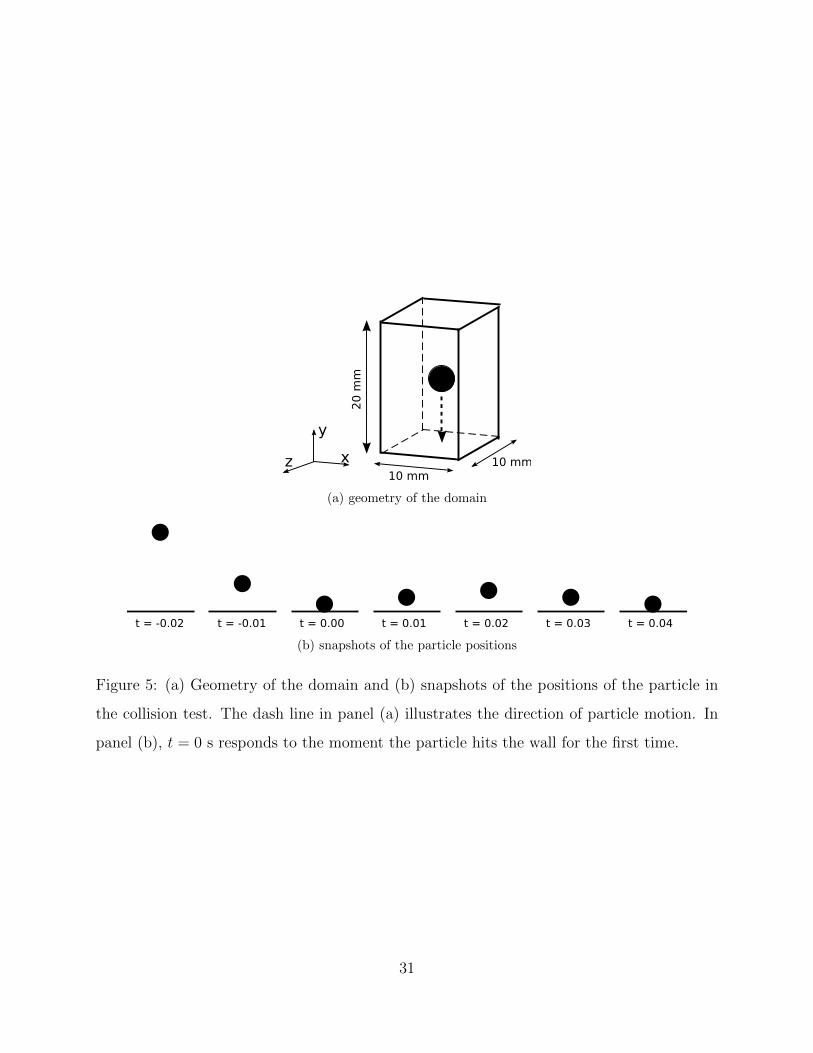
The geometry of the domain in the particle–wall collision test is shown in Figure 5 along

with the coordinate system. The parameters used in this case are detailed in Table 1.

Periodic boundary condition is applied at the boundaries in both x- and z-directions. In the

simulation, the fluid is quiescent initially and the particle falls in the vertical direction due

to the gravity force. The initial particle–wall distance is large enough so that the particle

accelerates to the terminal velocity before the collision occurs.

To test the influence of lubrication and added mass, the locations of the particle obtained

in the collision test are compared with the experimental results. The comparison is performed

at two different Stokes numbers, which is defined as:

St =ρpDpup9νfρf

=ρp

9ρfRep. (13)

In Fig. 6, the locations of the center of the sphere are plotted as a function of time. It

can be seen that the results obtained in the simulation that considered both lubrication and

added mass are consistent with the experimental measurements. Theoretically, added mass

force adds to the inertia of the particle, which leads to larger rebound height regardless

of the Stokes number. On the other hand, the lubrication depends on the viscous effect

and decreases with Stokes number. At St = 27, the viscous effect is large by definition.

Consequently, the locations of the particle predicted without lubrication are significantly

11

different from the experimental data. At St = 742, the viscous effects is small, so accounting

for lubrication at large Stokes number does not significantly influence the predictions of the

particle motions.

The prediction of the effective restitution coefficient using SediFoam in particle–wall

bouncing test is shown in Fig. 7. The effective restitution coefficient is defined as e =

ewater/eair, where ewater and eair are the restitution coefficients for the same collision occurs

in water and air, respectively. The amount of decrease of e from 1 denotes the influence of

lubrication and added mass in the collision. It can be seen in Fig. 7 that the predictions from

SediFoam agree favorably with the experimental data when the influence of lubrication and

added mass is considered. In contrast, the predictions without accounting for these forces

deviate significantly from experimental measurements by over-predicting the effective resti-

tution coefficients, particularly at small Stokes number. Accordingly, if sediment transport

occurs at relatively low Stokes number (Kidanemariam and Uhlmann, 2014b), the influence

of lubrication and added mass should be considered in CFD–DEM modeling of sediment

transport. Note that the calculation of lubrication incurs significant increase in computa-

tional costs. Consequently, lubrication are accounted for by using a smaller dry restitution

coefficient in the literature (Kidanemariam and Uhlmann, 2014a; Schmeeckle, 2014).

In summary, the influence of added mass and lubrication is important in the CFD–DEM

modeling of sediment transport. Additionally, the test cases validate the implementation of

the added mass force and lubrication force in SediFoam.

4.2. Case 2: Sediment Transport with 500 Particles

In this case, sediment transport at the boundary layer in the channel is studied. The

results obtained by using SediFoam are compared with the numerical benchmark to illustrate

the capability of the present solver. The averaging algorithm proposed by Sun and Xiao

(2015b) is applied to obtain the continuum Eulerian quantities from discrete particles. This

algorithm enables CFD–DEM simulation at the boundary layer where the size of CFD cells

is smaller than particles.

The numerical setup is based on the numerical benchmark studying the motion of 500

12

movable particles (Kempe et al., 2014). The geometry of the simulation is shown in Figure 8.

The dimensions of the domain, the mesh resolutions, and the fluid and particle properties

used are detailed in Table 1. The CFD mesh in the vertical (y-) direction is progressively

refined towards the bottom boundary. Periodic boundary condition is applied in both x-

and z-directions, no-slip wall condition is applied at the bottom in y-direction, and slip wall

condition is applied on the top in y-direction. The bulk Reynolds number Reb of the flow

in the channel is 3010. Six layers of fixed particles are arranged hexagonally to provide a

bottom boundary condition to the moving particles, as is shown in Fig. 8. In the coordinate

system, the top of the fixed particle bed is at y = 0. To obtain the profiles of fluid velocity

and Reynolds stresses, the simulations are averaged for 50 flow-through times, and spatial

average is performed in the horizontal domain. The bandwidth b used in the averaging

procedure is 2dp in width and thickness directions and dp in vertical direction.

The flow properties are presented in Fig. 9, including the streamwise velocity and Reynolds

stresses Rxx, Rxy, and Ryy. Fig. 9(a) shows that SediFoam is able to capture the decrease

of the fluid velocity in the near-wall boundary layer and within the bed, which is due to

the drag force of the sediment particles. The velocity profile near the particle bed at y = 0

is negative because of the diffusion effect of the averaging algorithm. Therefore, the diffu-

sion bandwidth in the vertical direction is taken as small as dp to reduce the effect of the

numerical diffusion. It can be seen from Fig. 9(b) to Fig. 9(d) that the predictions of differ-

ent components of Reynolds stresses from the present solver agree well with the numerical

benchmark. Compared with the flow that has no particles in the channel, SediFoam captures

the increase of the Reynolds stresses induced by the motion and collision of particles. It can

be seen that the overall agreement of results obtained by using SediFoam and DNS is good

for Rxx and Ryy. The discrepancy in Ryy is slightly larger than other components, which

may be attributed to the fact that CFD–DEM do not resolve the flow fluctuation at the

particle surface and cannot capture this quantity as good as the DNS.

Other quantities of interest in sediment transport include solid volume fraction and par-

ticle velocity. Figure 10 demonstrates the time-averaged probability density function (PDF)

13

and streamwise velocity of the particles at different vertical locations. It can be seen that

both the probability density function and streamwise velocity agree well with the results

in the numerical benchmark (Kempe et al., 2014). In the present simulation, the averaged

streamwise velocity of all particles up/ub is 0.28. Compared with the prediction 0.35 from

the numerical benchmark, the error is 20%. However, this error is insignificant since up is

proportional to the sediment transport rate, which varies significantly in the experimental

measurements. Therefore, the accuracy of CFD–DEM modeling is acceptable. It is notewor-

thy considering the fact that the total computational costs of CFD–DEM are much smaller

than the interface-resolved method. For this case, the number of CFD mesh in the present

simulation is 1.4× 105, whereas this number in the DNS simulation is 1.0× 108.

4.3. Case 3: Sediment Transport with O(105) Particles

The purpose of this simulation is to test the performance of the present code in the

simulation of larger problems of sediment transport. The results of both bed load sediment

transport and suspended sediment transport are demonstrated.

The layout of this case is similar to Case 2. The domain geometry, the mesh resolution,

and the properties of fluid and particles are detailed in Table 1. Periodic boundary condition

is applied in both x- and z-directions. Slip wall condition is applied at the top of the domain,

and no-slip wall condition is applied at the bottom. Three layers of solid particles are fixed

at the bottom to provide rough wall boundary condition for DEM simulation. The flow

velocities in five numerical simulations range from 0.3 m/s to 1.1 m/s. Each simulation

is performed for 50 flow-through times for time-averaging. The bandwidth b used in the

averaging procedure is 4dp in width and thickness directions and 2dp in vertical direction.

The geometry of this case is identical to the numerical tests using the same number of

particles by Schmeeckle (2014).

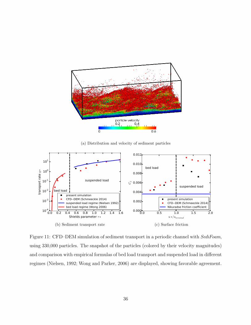
The averaged properties of sediment particles are presented in Fig. 11, including the

sediment transport rate and the friction coefficient. The sediment transport rate qsx is

obtained by multiplying the mean streamwise velocity of all particles by the total volume of

the particles, and divide it by the area of the horizontal plane. The non-dimensional sediment

14

fluxes q∗ = qsx/((ρs/ρf − 1)gd3p)1/2 at different Shields parameters τ∗ = ρfu

2∗/(ρs − ρf )gdp

are shown in Fig. 11(b). It can be seen in the figure that the sediment transport rates

agree favorably with the experimental data. Note that the q∗ in different regimes (i.e.,

bed load and suspended load) used different regression curves. It is worth mentioning that

the predictions of q∗ in suspended load regime using SediFoam are better than the results

obtained in the literature (Schmeeckle, 2014). This is because the drag force model in the

present simulations can better predict the motion of sediment particles since the influence

of εs is accounted for. The coefficient of friction of the surface is defined as Cf = u2∗/〈u〉2

and describes the roughness of the bed. Shown in Fig. 11(c), Cf obtained in the present

simulation are larger than the predictions by the law of the wall (i.e., Nikuradse value).

This increase in Cf is because the hydraulic roughness over a loose bed is larger in the

presence of movable particles. Note that the Cf predicted by SediFoam is slightly smaller

than the results predicted by Schmeeckle (2014). This is because Schmeeckle (2014) ignored

the volume fraction in the numerical simulation and used a smaller 〈u〉 when calculating Cf .

The spatially and temporally averaged profiles of solid volume fraction and flow velocity

are shown in Fig. 12. It can be seen from Fig. 12(a) that the εs above y/H = 0.2 is

approximately zero in the bed load regime. This is because the sediment particles are rolling

and sliding on the sediment bed in this regime. In the suspended load regime, the particles

are suspended in the flow due to turbulent eddies. Therefore, the εs above y/H = 0.2 is

much larger. The flow velocity profiles also vary at different regimes of sediment transport.

In the bed load regime, the height of the sediment bed is approximately 0.1H. The sediment

particles on the sediment bed are moving slowly in this regime. Hence, the streamwise flow

velocity decays rapidly under the sediment bed. In the suspended load regime, the flow

velocity at the sediment bed is more diffusive since the particles at the sediment bed are

moving more rapidly. Compared with the data obtained in the literature (Schmeeckle, 2014),

the overall agreement of solid volume fraction and flow velocity is satisfactory.

15

5. Scalability

The parallel efficiency is crucial to CFD–DEM solvers for simulations of large and complex

problems. In Section 5.1 and 5.2, the parallel efficiencies in the simulations of fluidized bed

and sediment transport are studied separately. This is because the setup, the flow regime,

and the behavior of particles are different between the two cases. The CPU time spent on

different parts of SediFoam is detailed in Section 5.3.

Both strong and weak scalability are studied in the parallel efficiency tests. The strong

scalability is to evaluate the performance of a solver for a constant sized problem being

separated by using more and more processors. The amount of the total work is constant

but the amount of communication work increases. The parallel efficiency of the strong

scalability test is Np0tp0/Npntpn, where Np0 and Npn are the number of processors employed

in the simulation of the baseline case and the test case, respectively; tp0 and tpn are the CPU

time. The speed-up is defined as tp0/tpn, which is the relative improvement of the CPU time

when solving the problem. The weak scalability evaluates the performance of a solver for

the problem with increasing number of processors. In the weak scalability test, the amount

of the work in different processors is the same. The parallel efficiency of the weak scalability

test is tp0/tpn. The scale-up is defined as Npntp0/tpn, which is the improvement in the scale

of the problem that SediFoam can solve.

5.1. Scalability of Fluidized Bed Simulation

The validation case of fluidized bed (Sun and Xiao, 2015a) is applied to test the parallel

efficiency of SediFoam. PCM-based averaging, which requires little computational cost, is

applied to reduce the influence of averaging algorithm. In the simulation of fluidized bed,

various numbers of processors are used from 4 to 256. The computational hours are calculated

by running 100 time steps in each case.

To test the strong scalability of the code for large-scale simulations, the numerical test

is performed using 5.3 million sediment particles and 1.3 million CFD cells. The domain

is 1056 mm × 600 mm × 240 mm in width (x-), height (y-), and transverse thickness (z-)

16

directions. The results obtained in the strong scalability test are shown in Fig. 13(a). It can

be seen that the parallel efficiency of SediFoam is close to 100% when employing less than

32 processors and is still as high as 85% when using 128 processors. However, the parallel

efficiency decreases to 52% when using 256 processors. In the test using 256 processors, the

number of sediment particles in each processor is as small as 20,000. From the results reported

in the literature, the parallel efficiency of SediFoam is approximately 15% higher than other

solvers when using this number of particles (Gopalakrishnan and Tafti, 2013). It is noted

in Fig. 13(a) that the parallel efficiency fluctuates when using 4 to 32 processors. This may

attributes to the fluctuation of the CPU time when solving the linear system. When using

different numbers of processors, the decomposition of the domain leads to different linear

systems and different converge rates when solving these linear systems. This fluctuation may

also be due to the variation of CPU cache or memory. The fluctuation of the CPU time can

also be seen in the speed-up curve, but the magnitude is small.

To test the weak scalability of SediFoam, 8.3×104 particles are located in each processor

with the dimensions of 66 mm × 600 mm × 60 mm in width (x-), height (y-), and transverse

thickness (z-) directions. The numbers of processors vary from 4 to 256, and thus the total

numbers of particles vary from 0.3 million to 21 million. It can be seen in Fig. 13(b) that

good weak scalability is observed. The parallel efficiency is close to 100% when using less

than 32 processors and gradually decreases to 61% when using 256 processors. Therefore,

the ultimate scale-up of the code by using 256 processors is as large as 156.

5.2. Scalability of Sediment Transport Simulation

Simulations of sediment transport cases are performed to test the parallel efficiency of

SediFoam when the number of CFD mesh is larger than the number of particles. The

diffusion-based averaging algorithm is applied in the simulations. The numbers of processors

used vary from 8 to 512.

To test the strong scalability of the code for large-scale simulations, we expanded the

domain in Case 3 to be 480 mm × 40 mm × 480 mm in width (x-), height (y-), and

transverse thickness (z-) directions. The numbers of sediment particles and CFD cells are

17

10 million and 13 million, respectively. It can be seen in Fig. 14(a) that good scalability

and parallel efficiency are obtained in this test. The parallel efficiency is close to 100% when

using less than 64 processors and decreases to 52% when using 512 processors.

To test the weak scalability for sediment transport, 7.8 × 104 particles are located in

each processor with the dimension of 60 mm × 40 mm × 30 mm in width (x-), height

(y-), and transverse thickness (z-) directions. The total numbers of particles vary from

0.6 million to 40 million. The parallel efficiency and the scale-up of SediFoam are shown

in Fig. 13(b). Compared with the results obtained in the fluidized bed test, the parallel

efficiency in sediment transport test is lower. This is because solving the fluid equations is

difficult in parallel when the number of CFD cells is very large.

In summary, although the parallel efficiency of SediFoam in the sediment transport cases

is smaller than the fluidized bed cases, the general efficiency is still satisfactory compared to

other CFD–DEM solvers (Amritkar et al., 2012; Capecelatro and Desjardins, 2013; Gopalakr-

ishnan and Tafti, 2013). Moreover, simulations of O(107) number of particles are performed,

which demonstrates the capability of SediFoam in the simulation of relatively large scale

problems.

5.3. Parallel performance of different components

The investigation of the computational costs of different components in SediFoam is

detailed in this section. The study consists of both simulations of fluidized bed and sediment

transport, using the results obtained in the tests of Section 5.1 and 5.2. The time spent on the

CFD module, the DEM module, the coupling between the two modules, and the averaging

algorithm are discussed.

The results obtained in the fluidized bed simulation are shown in Table. 2. It can be

seen in the table that the most time-consuming process is solving the collision between the

particles, which accounts for 46% to 76% of the total costs. Solving the fluid equations is the

second most time-consuming process, which takes 21% to 31% of the total computational

costs for both strong scaling and weak scaling. It is noted that the coupling process takes

less than 2% of the total costs when using less than 64 processors. However, the proportion

18

of this part increases significantly to about 20% when using 256 processors. This is because

the time spent on the inter-processor communication increases due to the increase number

of processors used in the simulation. This increase can also be seen in the weak scaling test

for both the CFD and DEM modules, which are well-established solvers with good parallel

efficiency.

The computational costs of different components in the sediment transport simulation are

detailed in Table. 3. Since the number of CFD cells is larger than the number of sediment

particles, the computational costs of the CFD module are larger than the DEM module.

It can be seen that the proportion of CFD part is approximately 21% to 48% the total

computational costs for both strong scaling and weak scaling tests. The DEM part accounts

for about 17% to 37% of the total costs. It is noted that the computational overhead of

the averaging also accounts for 20% to 33% of the total computational overhead. The time

spent on the coupling is less than 2% of the total time when using less than 128 processors.

However, when using as many as 512 processors the time spend on the communication

increases significantly.

6. Conclusion

In this work, the parallelized open-source CFD–DEM solver SediFoam is developed with

emphasis on the simulation of sediment transport. The CFD and DEM modules are based

on OpenFOAM and LAMMPS, respectively. The communication between the modules is

implemented using parallel algorithm to enable the simulation of large-scale problems.

Numerical validations are performed to test the capability of the present solver. The

single particle sedimentation test demonstrates the importance of added mass and lubrication

in CFD–DEM simulations. In the numerical simulations of with 500 sediment particles, the

fluid and particle properties obtained are consistent with the results obtained by interface-

resolved method. This indicates the accuracy of SediFoam is desirable. The numerical

simulation using O(105) particles demonstrates the capability of SediFoam in the simulation

of various regimes in sediment transport.

19

Parallel efficiency tests are conducted to investigate the scalability of SediFoam. From

the test, the scalability of SediFoam is satisfactory compared with other existing CFD–DEM

solvers. This demonstrates that SediFoam is a desirable solver for the simulation of sediment

transport of large-scale and complex problems.

7. Acknowledgment

The computational resources used for this project are provided by the Advanced Research

Computing (ARC) of Virginia Tech, which is gratefully acknowledged. We also thank Dr. Jin

Sun at University of Edingburgh, who helped improve the quality of the manuscript through

technical discussions. Moreover, we thank Dr. Calantoni for the discussions, which helped

with the numerical simulations in the present paper. The authors gratefully acknowledge

partial funding of graduate research assistantship from the Institute for Critical Technology

and Applied Science (ICTAS, grant number 175258) in this effort.

References

Amritkar, A., Tafti, D., Liu, R., Kufrin, R., Chapman, B., 2012. OpenMP parallelism for

fluid and fluid–particulate systems. Parallel Computing 38 (9), 501–517.

Anderson, T., Jackson, R., 1967. A fluid mechanical description of fluidized beds: Equations

of motion. Industrial and Chemistry Engineering Fundamentals 6, 527–534.

Ball, R. C., Melrose, J. R., 1997. A simulation technique for many spheres in quasi-static

motion under frame-invariant pair drag and Brownian forces. Physica A: Statistical Me-

chanics and its Applications 247 (1), 444–472.

Calantoni, J., Holland, K. T., Drake, T. G., 2004. Modelling sheet-flow sediment transport

in wave-bottom boundary layers using discrete-element modelling. Philosophical Transac-

tions of Royal Society of London: Series A 362, 1987–2002.

Capecelatro, J., Desjardins, O., 2013. An Euler–Lagrange strategy for simulating particle-

laden flows. Journal of Computational Physics 238, 1–31.

20

Cundall, P., Strack, D., 1979. A discrete numerical model for granular assemblies.

Geotechnique 29, 47–65.

Deb, S., Tafti, D. K., 2013. A novel two-grid formulation for fluid–particle systems using the

discrete element method. Powder Technology 246, 601–616.

Di Felice, R., 1994. The voidage function for fluid–particle interaction systems. International

Journal of Multiphase Flow 20 (1), 153–159.

Drake, T. G., Calantoni, J., 2001. Discrete particle model for sheet flow sediment transport

in the nearshore. Journal of Geophysical Research: Oceans (1978–2012) 106 (C9), 19859–

19868.

Duran, O., Andreotti, B., Claudin, P., 2012. Numerical simulation of turbulent sediment

transport, from bed load to saltation. Physics of Fluids (1994-present) 24 (10), 103306.

Ebrahimi, M., 2014. CFD–DEM modelling of two-phase pneumatic conveying with experi-

mental validation. Ph.D. thesis.

Eppinger, T., Seidler, K., Kraume, M., 2011. DEM-CFD simulations of fixed bed reactors

with small tube to particle diameter ratios. Chemical Engineering Journal 166 (1), 324–

331.

Feng, Y., Yu, A., 2004. Assessment of model formulations in the discrete particle simulation

of gas-solid flow. Industrial & engineering chemistry research 43 (26), 8378–8390.

Fries, L., Antonyuk, S., Heinrich, S., Palzer, S., 2011. DEM–CFD modeling of a fluidized

bed spray granulator. Chemical Engineering Science 66 (11), 2340–2355.

Furbish, D., Schmeeckle, M., 2013. A probabilistic derivation of the exponential-like distri-

bution of bed load particle velocities. Water Resources Research 49 (3), 1537–1551.

Garg, R., Galvin, J., Li, T., Pannala, S., 2012. Open-source MFIX-DEM software for gas–

solids flows: Part I–Verification studies. Powder Technology 220, 122–137.

21

Gondret, P., Lance, M., Petit, L., 2002. Bouncing motion of spherical particles in fluids.

Physics of Fluids (1994-present) 14 (2), 643–652.

Goniva, C., Kloss, C., Pirker, S., 2009. Towards fast parallel CFD–DEM: an open-source

perspective. In: Proc. of Open Source CFD International Conference. November 12-13,

Barcelona, Spain.

Gopalakrishnan, P., Tafti, D., 2013. Development of parallel DEM for the open source code

MFIX. Powder Technology 235, 33–41.

Gupta, P., 2015. Verification and validation of a DEM–CFD model and multiscale modelling

of cohesive fluidization regimes. Ph.D. thesis.

Hockney, R., Goel, S., Eastwood, J., 1974. Quiet high-resolution computer models of a

plasma. Journal of Computational Physics 14 (2), 148–158.

Issa, R. I., 1986. Solution of the implicitly discretised fluid flow equations by operator-

splitting. Journal of Computational Physics 62 (1), 40–65.

Jajcevic, D., Siegmann, E., Radeke, C., Khinast, J. G., 2013. Large-scale CFD–DEM simu-

lations of fluidized granular systems. Chemical Engineering Science 98, 298–310.

Jasak, H., 1996. Error analysis and estimation for the finite volume method with applications

to fluid flows. Ph.D. thesis, Imperial College London (University of London).

Kafui, K., Thornton, C., Adams, M., 2002. Discrete particle–continuum fluid modelling of

gas–solid fluidised beds. Chemical Engineering Science 57 (13).

Kempe, T., Vowinckel, B., Frohlich, J., 2014. On the relevance of collision modeling for

interface-resolving simulations of sediment transport in open channel flow. International

Journal of Multiphase Flow 58, 214–235.

Kidanemariam, A. G., Uhlmann, M., 2014a. Direct numerical simulation of pattern formation

in subaqueous sediment. Journal of Fluid Mechanics 750, 1–13.

22

Kidanemariam, A. G., Uhlmann, M., 2014b. Interface-resolved direct numerical simulation

of the erosion of a sediment bed sheared by laminar channel flow. International Journal of

Multiphase Flow 67, 174–188.

Li, T., Garg, R., Galvin, J., Pannala, S., 2012. Open-source MFIX-DEM software for gas-

solids flows: Part II-validation studies. Powder Technology 220, 138–150.

Nielsen, P., 1992. Coastal bottom boudary layers and sediment transport. World Scientific

Publishing.

OpenCFD, 2013. OpenFOAM User Guide. See also http://www.opencfd.co.uk/openfoam.

Plimpton, J., 1995. Fast parallel algorithms for short-range molecular dynamics. Journal of

Computational Physics 117, 1–19, see also http://lammps.sandia.gov/index.html.

Saffman, P., 1965. The lift on a small sphere in a slow shear flow. Journal of fluid mechanics

22 (02), 385–400.

Schmeeckle, M. W., 2014. Numerical simulation of turbulence and sediment transport of

medium sand. Journal of Geophysical Research: Earth Surface 119, 1240–1262.

Spogis, N., 2008. Multiphase modeling using EDEM–CFD coupling for FLUENT. CFD OIL,

18–19.

Sun, J., Battaglia, F., Subramaniam, S., 2007. Hybrid two-fluid DEM simulation of gas-solid

fluidized beds. Journal of Fluids Engineering 129 (11), 1394–1403.

Sun, J., Xiao, H., Gao, D., 2009. Numerical study of segregation using multiscale models.

International Journal of Computational Fluid Dynamics 23, 81–92.

Sun, R., Xiao, H., 2015a. Diffusion-based coarse graining in hybrid continuum–discrete

solvers: Applications in CFD–DEM. International Journal of Multiphase Flow 72, 233–

247.

23

Sun, R., Xiao, H., 2015b. Diffusion-based coarse graining in hybrid continuumdiscrete solvers:

Theoretical formulation and a priori tests. International Journal of Multiphase Flow 77,

142 – 157.

Syamlal, M., Rogers, W., O’Brien, T., 1993. MFIX documentation: Theory guide.

Tech. rep., National Energy Technology Laboratory, Department of Energy, see also

http://www.mfix.org.

Tsuji, Y., Kawaguchi, T., Tanaka, T., 1993. Discrete particle simulation of two-dimensional

fluidized bed. Powder Technolgy 77 (79-87).

van Rijn, L., 1984. Sediment transport, part I: Bed load transport. Journal of hydraulic

engineering 110 (10), 1431–1456.

Wang, R.-Q., Law, A. W.-K., Adams, E. E., 2014. Large-Eddy Simulation (LES) of settling

particle cloud dynamics. International Journal of Multiphase Flow 67, 65–75.

Wen, C., Yu, Y., 1966. Mechanics of fluidization. In: Chem. Eng. Prog. Symp. Ser. Vol. 62.

p. 100.

Wong, M., Parker, G., 2006. Reanalysis and correction of bed-load relation of Meyer–Peter

and Muller using their own database. Journal of Hydraulic Engineering 132 (11), 1159–

1168.

Wu, C. L., Ayeni, O., Berrouk, A. S., Nandakumar, K., 2014. Parallel algorithms for CFD–

DEM modeling of dense particulate flows. Chemical Engineering Science 118, 221–244.

Xiao, H., Sun, J., 2011. Algorithms in a robust hybrid CFD–DEM solver for particle-laden

flows. Communications in Computational Physics 9, 297–323.

Zhou, Z., Kuang, S., Chu, K., Yu, A., 2010. Discrete particle simulation of particle–fluid flow:

model formulations and their applicability. Journal of Fluid Mechanics 661, 482–510.

24

Zhu, H. P., Yu, A. B., 2002. Averaging method of granular materials. Physical Review E

66 (2), 021302.

Table 1: Parameters of the numerical simulations.

Case 1 Case 2 Case 3

domain dimensions

width (Lx) (mm) 100 58.4 120

height (Ly) (mm) 200 13.5 40

transverse thickness (Lz) (mm) 100 29.2 60

mesh resolutions

width (Nx) 10 52 140

height (Ny) 20 102 65

transverse thickness (Nz) 10 26 60

particle properties

total number 1 500 3.3× 105

diameter dp (mm) 6 1.12 0.5

density ρs (×103 kg/m3) 2.5/7.8 (sand/steel) 2.0 2.5

particle stiffness coefficient (N/m) 800 800 800

normal restitution coefficient 0.97 0.97 0.01

coefficient of friction 0.1 0.1 0.1

fluid properties

viscosity ν (×10−6 m2/) 1.0∼5.4 1.0 1.0

density ρf (×103 kg/m3) 1.0 1.0 1.0

25

Table 2: Breakdown of computational costs associated with different parts of fluidized bed

simulations. For the both tests, the CPU times presented here are normalized by the time

spent on the CFD part of the case using 256 processors.

Np = 4 16 64 256

strong scaling

CFD 33.6(28%) 7.7 (27%) 1.9(23%) 1.0(28%)

DEM 89.0(71%) 20.4(72%) 5.9(74%) 1.6(46%)

coupling 3.1 (2%) 0.4 (1%) 0.2(3%) 0.9(21%)

total 125.7 28.5 8.0 3.6

weak scaling

CFD 0.4(21%) 0.3(27%) 0.7(26%) 1.0(31%)

DEM 1.6(76%) 1.7(72%) 1.7(70%) 1.9(56%)

coupling 0.1(3%) 0.0(1%) 0.1(4%) 0.4(13%)

total 2.1 2.1 2.5 3.3

26

Table 3: Breakdown of computational costs associated with different parts of sediment

transport simulations. For the both tests, the CPU times presented here are normalized by

the time spent on the CFD part of the case using 8 processors.

Np = 8 32 128 512

strong scaling

CFD 74.4(47%) 20.1(47%) 4.4(45%) 1.0(21%)

DEM 35.8(23%) 10.1(23%) 2.8(29%) 0.8(17%)

averaging 45.7(29%) 12.9(30%) 2.5(25%) 1.4(29%)

coupling 1.2 (0%) 0.2 (0%) 0.1(1%) 1.6(33%)

total 157.0 43.2 8.0 4.7

weak scaling

CFD 0.2(29%) 0.3(37%) 0.6(45%) 1.0(48%)

DEM 0.3(37%) 0.3(36%) 0.4(29%) 0.4(20%)

averaging 0.3(33%) 0.2(27%) 0.3(25%) 0.4(20%)

coupling 0.0(1%) 0.0(1%) 0.0(1%) 0.2(11%)

total 0.8 0.9 1.4 2.1

27

Solve fluid equations

Update fluid-particle interaction force

Simulate particle motion

Solve averaging equations

Next time step

CFD module(OpenFOAM)

DEM module(LAMMPS)

Update particleinformation

Figure 1: The block diagram of the code.

Processor 1 Processor 2 Processor 3

Figure 2: Decomposition of the computational domain in CFD–DEM simulation. Different

colors in the CFD mesh denotes different subdomains in the CFD module, while the bound

boxes of different colors denotes different subdomains in the DEM module.

28

DEM subdomainfor processor (a)

CFD subdomainfor processor (1)

CFD subdomainfor processor (2)

CFD subdomainfor processor (3)

DEM subdomainfor processor (b)

DEM subdomainfor processor (c)

Figure 3: The geometry of a representative CFD–DEM case that the decompositions of the

CFD and the DEM modules are different. The blue lines are the CFD mesh and the black

dash lines illustrate the subdomains of the CFD module; the red lines are the subdomains

of the DEM module.

29

1,aProcessor I

1,a

1,b

2,a

2,a2,a

2,b

(a) Evolve particles in DEM module (b) DEM module find non-local particle

(c) Transfer data (d) Update particle information in CFD module

3,a

2,b

3,b

3,b

1,c 1,c

1,c

2,c 3,c 3,c

3,c

1,a

1,a

1,b

2,a

2,a2,a

2,b

3,a

2,b

3,b

3,b

1,c 1,c

1,c

2,c 3,c 3,c

3,c

1,a

1,a

1,b

2,a

2,a2,a

2,b

3,a

2,b

3,b

3,b

1,c 1,c

1,c

2,c 3,c 3,c

3,c

1,a

1,a1,b

2,a

2,a2,a

2,b

3,a

2,b

3,b

3,b

1,c 1,c

1,c

2,c

3,c 3,c

3,c

Processor II

Processor III

Processor I

Processor II

Processor III

Processor I

Processor II

Processor III

Processor I

Processor II

Processor III

Figure 4: Inter-processor communication of the particle information. Each circle represents

a sediment particle in the simulation. Number 1, 2, and 3 indicates the processor that stores

the data of the particle in the CFD module; character “a”, “b” and “c” denote the processor

that store the data of the particle in the DEM module.

30

20

mm

xz

y

10 mm10 mm

(a) geometry of the domain

t = -0.02 t = -0.01 t = 0.00 t = 0.01 t = 0.02 t = 0.03 t = 0.04

(b) snapshots of the particle positions

Figure 5: (a) Geometry of the domain and (b) snapshots of the positions of the particle in

the collision test. The dash line in panel (a) illustrates the direction of particle motion. In

panel (b), t = 0 s responds to the moment the particle hits the wall for the first time.

31

0.02 0.00 0.02 0.04 0.06 0.08 0.10t

0.000

0.005

0.010

0.015

0.020

h

drag onlydrag + added massdrag + added mass + lubricationexperimental (Gondret 2002)

(a) St = 27

0.1 0.0 0.1 0.2 0.3t

0.00

0.02

0.04

0.06

0.08

0.10

h(b) St = 742

Figure 6: The positions of the particle plotted as a function of time in the particle–wall

bouncing test. The influence of lubrication and added mass are considered at Stokes number

(a) St = 27 and (b) St = 742.

100 101 102 103 104 105

Stokes number

0.0

0.2

0.4

0.6

0.8

1.0

eff

ect

ive r

est

ituti

on c

oeff

icie

nt

without added mass and lubrication (steel)

with added mass and lubrication (steel)

without added mass and lubrication (sand)

with added mass and lubrication (sand)

experiment (Gondret 2002)

Figure 7: The influence of lubrication and added mass on the effective restitution coefficient

in particle–wall collisions for different particles at different Stokes numbers.

32

Figure 8: Layout of sediment transport simulation according to Kempe et al. (2014). The

white particles are fixed on the bottom; the gray particles are movable.

33

0.0 0.5 1.0 1.5<u>/Ub

0.2

0.0

0.2

0.4

0.6

0.8

1.0

y/H

present simulationDNS (Kempe et al. 2014)

0.00 0.02 0.04 0.06 0.08 0.10Rxx/U

2b

0.2

0.0

0.2

0.4

0.6

0.8

1.0

y/H

0.0100.0080.0060.0040.0020.000Rxy/U

2b

0.2

0.0

0.2

0.4

0.6

0.8

1.0

y/H

0.000 0.002 0.004 0.006 0.008 0.010Ryy/U

2b

0.2

0.0

0.2

0.4

0.6

0.8

1.0

y/H

Figure 9: Comparison of mean velocity 〈u〉 and Reynolds stresses Rxx, Rxy, and Ryy along

the wall normal direction (y) obtained by using SediFoam with the DNS results (Kempe

et al., 2014). The mean location of the particle bed is at y = 0.

34

0.0 0.5 1.0 1.5 2.0 2.5y/D

0.00

0.05

0.10

0.15

P(yp)

present simulationDNS (Kempe et al. 2014)

0.0 0.5 1.0 1.5 2.0 2.5y/D

0.00

0.25

0.50

0.75

1.00

<up>/U

b

Figure 10: Probability density function and streamwise velocity in the simulation of 500

movable particles.

35

(a) Distribution and velocity of sediment particles

0.0 0.2 0.4 0.6 0.8 1.0 1.2 1.4 1.6Shields parameter τ ∗

10-4

10-3

10-2

10-1

100

101

transp

ort

rate

q∗

bed load

suspended load

present simulationCFD--DEM (Schmeeckle 2014)suspended load regime (Nielsen 1992)bed load regime (Wong 2006)

(b) Sediment transport rate

0.0 0.5 1.0 1.5 2.0u ∗/uterminal

0.000

0.002

0.004

0.006

0.008

0.010

0.012

Cf

bed load

suspended load

present simulationCFD--DEM (Schmeeckle 2014)Nikuradse friction coefficient

(c) Surface friction

Figure 11: CFD–DEM simulation of sediment transport in a periodic channel with SediFoam,

using 330,000 particles. The snapshot of the particles (colored by their velocity magnitudes)

and comparison with empirical formulas of bed load transport and suspended load in different

regimes (Nielsen, 1992; Wong and Parker, 2006) are displayed, showing favorable agreement.

36

10-6 10-5 10-4 10-3 10-2 10-1 100

solid volume fraction

10-3

10-2

10-1

100y/H <u>=0.3 m/s

<u>=0.5 m/s<u>=0.7 m/s<u>=0.9 m/s<u>=1.1 m/s

(a) Solid volume fraction εs

0 5 10 15 20<u>/u ∗

10-3

10-2

10-1

100

y/H

(b) Streamwise flow velocity

Figure 12: The solid volume fraction εs and streamwise flow velocity of different flow veloci-

ties. The blue lines are the simulations in bed load regime; the red lines are the simulations

in suspended load regime.

0 50 100 150 200 250number of CPUs

0.0

0.2

0.4

0.6

0.8

1.0

effic

ienc

y

parallel efficiency

0

50

100

150

200

250

300

para

llel s

peed

-up

idealactural speed-up

(a) strong scaling

0 50 100 150 200 250number of CPUs

0.0

0.2

0.4

0.6

0.8

1.0

effic

ienc

y

0

50

100

150

200

250

300

para

llel s

cale

-up

(b) weak scaling

Figure 13: The parallel efficiency of SediFoam for strong scaling and weak scaling in flu-

idized bed. The test case employs up to 21 million sediment particles using up to 256

CPU cores. The simulation with the smallest number cores is regarded as base case

when computing speed-up. Tests are performed on Virginia Tech’s BlueRidge cluster.

(http://www.arc.vt.edu/)

37

0 100 200 300 400 500number of CPUs

0.0

0.2

0.4

0.6

0.8

1.0

effic

ienc

y

0

100

200

300

400

500

600

para

llel s

peed

-up

(a) strong scaling

0 100 200 300 400 500number of CPUs

0.0

0.2

0.4

0.6

0.8

1.0

effic

ienc

y

0

100

200

300

400

500

600

para

llel s

cale

-up

(b) weak scaling

Figure 14: The parallel efficiency of SediFoam for strong scaling and weak scaling in sedi-

ment transport. The test case employs up to 40 million sediment particles using up to 512

CPU cores. The simulation with the smallest number cores is regarded as base case when

computing speed-up.

38