University of Newcastle upon Tyne Department of Computing Science An Investigation of Collocation Algorithms for Solving Boundary Value Problems System of ODEs A thesis submitted in partial fulfilment of the requirements for the degree of Doctor of Philosophy in Computing Science Edy Hermansyah September 2001 NrWCASTLE UNIV[R~ITV LIBRARV ----------------------- ----- 201 09968 6 ---------------------------- ~(WCASTLE UPON TYNE 418RA~~//
Transcript
University of Newcastle upon Tyne
Department of Computing Science
An Investigation of Collocation Algorithmsfor Solving Boundary Value Problems
System of ODEs
A thesis submitted in partial fulfilmentof the requirements for the degree of
I would like to express my special thanks to Dr Kenneth Wright, for having
suggested this subject of research. I am very grateful to him for his valuable
guidance, advice and encouragement during development of this thesis. He has
demonstrated a great deal of patience during his time as my supervisor, and offered
innumerable valuable insight into my research topic. lowe Dr Kenneth Wright
a significant debt for this work, and I fear that it may be one I will never be able to
repay sufficiently.
My deepest gratitude goes to Dr John Lloyd and Dr Chris Phillips, both member of
my thesis committee, for their valuable inputs and their very helpful comments
throughout this work.
Many staff members of the Department of Computing Science deserve my gratitude.
In particular, I wish to acknowledge Ms Shirley Craig who helped me so much in
obtaining bibliographical references for this research.
Financial support has been provided by The Higher Education Project - University of
Bengkulu (Proyek Pengembangan Sebelas Lembaga Pendidikan Tinggi, P2SLPT-
Universitas Bengkulu).
The last but not the least, I am very grateful to my family in Palembang and
Bengkulu who gave me a lot encouragement in my most difficult time. My very
especial thanks are due to Ika, Tity and her husband, Yanti and her husband, Donga
Yassin and his wife, Pak Cik B and his wife, my brothers Co , Oji and Man, as well
as to Risma and her husband.
This thesis is dedicated to Sri Wahyuni who gave me almost every things needed
when I attempted to recognize myself; and also to Annisa si Kanda, Amelia si Intan,
and Afif si Willy. mang kimang kiming anak anak ayah ...
Abstract
This thesis is concerned with an investigation and evaluation of collocation
algorithms for solving two-point boundary value problems for systems of ordinary
differential equations. An emphasis is on developing reliable and efficient adaptive
mesh selection algorithms in piecewise collocation methods.
General background materials including basic concepts and descriptions of the
method as well as some functional analysis tools needed in developing some error
estimates are given at the beginning. A brief review of some developments in the
methods to be used is provided for later referencing.
By utilising the special structure of the collocation matrices, a more compact block
matrix structure is introduced and an algorithm for generating and solving the
matrix is proposed. Some practical aspects and computational considerations of
matrices involved in the collocation process such as analysis of arithmetic
operations and amount of memory spaces needed are considered. An examination of
scaling process to reduce the condition number is also presented.
A numerical evaluation of some error estimates developed by considering the
differential operator, the related matrices and the residual is carried out. These
estimates are used to develop adaptive mesh selection algorithms, in particular as a
cheap criterion for terminating the computation process.
Following a discussion on mesh selection strategies, a criterion function for use in
adaptive algorithms is introduced and a numerical scheme to equidistributing values
of the criterion function is proposed. An adaptive algorithm based on this criterion
is developed and the results of numerical experiments are compared with those using
some well known criterion functions. The various examples are chosen in such a way
that they include problems with interior or boundary layers.
In addition, an algorithm has been developed to predict the necessary number of
subintervals for a given tolerance, with the aim of improving the efficiency of the
whole process.
Using a good initial mesh in adaptive algorithms would be expected to provide some
further improvement in the algorithms. This leads to the idea of locating the layer
regions and determining suitable break points in such regions before the numerical
process. Based on examining the eigenvalues of the coefficient matrix in the
differential equation in the specified interval, using their magnitudes and rates of
change, the algorithms for predicting possible layer regions and estimating the
number of break points needed in such regions are constructed. The effectiveness of
these algorithms is evaluated by carrying out a number of numerical experiments.
The final chapter gives some concluding remarks of the work and comment on results
of numerical experiments. Certain possible improvements and extensions for further
research are also briefly given.
ii
Contents
Page
AbstractContents iii
Chapter 1 Introduction and Preliminaries........................................ 11.1 General Background 11.2 Collocation Methods 2
1.2.1 Global and Piecewise Polynomial Solutions 21.2.2 Adaptive Mesh Selection Algorithms 6
1.3 A im 61.4 Structure of the Thesis 7
Chapter 2 Review of Some Developments in the Collocation Methods 92.1 Introduction 92.2 Collocation and Projection Method 102.3 Error Bounds for Collocation Solutions 122.4 Brief Review of Some Other Developments 16
Chapter 3 Developing Algorithms for Solving the Collocation Matrix ... .... 203.1 Introduction 203.2 Computational Consideration of Collocation Matrix 21
3.2.1 Scaling Operation and Condition Number 223.2.2 Some Results of Numerical Experiments 25
3.3 Basic Structure of the Collocation Matrix 293.4 Block Matrix Representation 31
3.4.1 Reduction to Block Matrix Form 323.4.2 Analysis of Works and Amount of Memory Spaces 35
3.5 Computationallllustrations 37
Chapter 4 Numerical Evaluation of the Error Estimates 414.1 Introduction 414.2 Behaviour of the Collocation Matrix Norms 434.3 The Residual 444.4 The Error Estimates 524.5 Numerical Experiments 554.6 Numerical Evaluation of the Estimate E* for Stiff BVPs 66
III
Chapter 5 Adaptive Mesh Selection Strategies for CollocationAlgorithms 705.1 Introduction 705.2 Some Basic Concepts 71
5.2.1 Structure of Adaptive Mesh Selection Algorithms 715.2.2 Error Equidistribution and Criterion Function 735.2.3 Mesh Placement and Mesh Subdivision Algorithms 75
5.3 Some Well Known Criterion Functions 765.3.1 Maximum Residual 765.3.2 De Boor's Algorithm 775.3.3 Other Criterion Functions 79
5.4 Using rh, as the Criterion Function 805.4.1 Motivation for Using rh, as the Criterion Function 805.4.2 Developing the Scheme for Equidistributing the
Terms rh, 825.5 Numerical Results 85
Chapter 6 Predicting the Number of Subintervals Needed in theCollocation Processes 966.1 Introduction 966.2 Mesh Placement Algorithms 986.3 Estimating the Constant C 1016.4 Practical Implementation 1026.5 Mesh Subdivision Algorithms 1126.6 Numerical Illustrations 114
Chapter 7 Locating the Layer Regions and Estimating Their InitialMesh Points............................................................... 1217.1 Nature of Stiffness 1217.2 Eigenvalues for Predicting the Layer Locations 1237.3 Determining the Width of Layers 1317.4 Initial Mesh Points in the Layer Regions 1337.5 Numerical Implementations 137
Piecewise collocation methods not only allow great flexibility in placement of the
collocation points but also provide a wider choice of basis functions. Ahmed [1],
Gerrard [26] and Seleman [48] in their theses have used local Chebyshev
polynomials. The use of B-Spline can be found in Ascher et al. [8], de Boor [22] and
Dodson [24]. Hermite polynomials were used by de Boor and Swartz [23]. Ascher
et al. [8] also used monomial basis functions and further application of this kind of
basis can be found in Ascher [6] and Ascher et al. [10].
As mentioned earlier, to guarantee the convergence of the global collocation
methods the collocation points should be chosen from known orthogonal
polynomials. In most references mentioned the collocation points are either the zeros
of Chebyshev polynomial (Chebyshev zeros) or the zeros of Legendre polynomials
(Gauss points). A discussion of piecewise collocation based on Lobatto and Radau
points can be found in Ascher and Bader [7], while Wright [56] considered the use of
zeros of the ultra-spherical polynomials which is a generalisation of the choice of
collocation points which includes Chebyshev and Gauss points.
5
Chapter 1 I n t rod u c ti 0 n
1.2.2 Adaptive Mesh Selection Algorithms
There are some problems of the form 0.3) in which a collocation method using
only uniform meshes will be either inefficient or it will not work at all. In this
category will be most problems whose solutions (or their derivatives) have very sharp
gradients such as problems with boundary layers.
Choosing a good mesh is essential if a method is to be efficient, in the sense a
sufficiently accurate solution should be obtained as inexpensively as possible, for
problems with solution having a narrow region of rapid change such as occur even
for the very simple problems of this type.
Since the collocation methods on a computer involve repetitions of some
computation processes to achieve a desired approximate solution, two issues arise.
Firstly a reliable strategy in choosing the break points in a mesh is needed; secondly
a good initial mesh to start the collocation process is also important. The first issue
corresponds to adaptive mesh selection, where the approximate solution and the
mesh are repeatedly updated until prescribed error criteria are deemed satisfied. The
second one relate to initial consideration of the problem itself, possibly by a
preliminary mathematical analysis, for instance an initial solution profile can be used
to construct an initial mesh, the stiffness may give some hint that in some regions we
should place more points than other regions.
Despite the tremendous importance of mesh placement strategies in collocation
methods, very little has been carried out about the problem of choosing those
nonuniform meshes in the way most adequate for a given problem. Beside the most
outstanding contribution of de Boor [22], the other references include Ahmed [1],
Russell and Christiansen [45], Seleman [48] and Wright et al. [60].
1.3 A im
This thesis is primarily concerned with developing some reliable, in terms of
accuracy and efficiency, collocation algorithms for solving boundary value problems
for system of ordinary differential equations. In particular we shall investigate a
6
Chapter 1 I n t rod u c ti 0 n
variety of mesh selection strategies for piecewise collocation methods. An efficient
criterion function to be used in adaptive mesh selection algorithms will be introduced
and some results of numerical comparisons will be discussed, followed by drawing
some conclusion.
When attempting to develop an adaptive mesh selection algorithm, at least we
deal with the process of
• choosing an initial mesh
• setting up and solving system of linear equations
• constructing a new mesh for the next stage
• a criterion for terminating the process.
In this work all the above will be considered in detail, and some discussion and
evaluation based on numerical experiment will be presented.
Some error estimate processes based on consideration of the differential operator
involved and on the residual will be evaluated in numerical experiments. One of
these estimates will then be used in constructing a new mesh and for terminating the
computation process.
1.4 Structure of the Thesis
In chapter 2, the boundary value problem of the form (1.3) is transformed and
defined in operator form. This enables us to relate it to the theory of the projection
method needed in developing our work. Subsequently, a brief review of recent
developments in collocation algorithms is presented.
Chapter 3 deals with developing algorithms for solving the system of linear
equations generated in the collocation process. Some computational considerations
such as column scaling schemes for reducing the condition number of the matrix
involved in the equation system will be examined and some practical results will be
displayed and discussed. Analysis of arithmetic operations and amount of memory
needed for both full matrix representation and developed block matrix are considered
and then followed by carrying out numerical comparisons.
7
Chapter 1 I n t rod u c ti 0 n
Some numerical evaluations of the error estimates are presented in chapter 4.
Particular attention is given to boundary value problems having severe layers, from
which we observe the reliability of the error estimates when dealing with these
problems.
Chapter 5 consists of investigation of some adaptive mesh selection algorithms
and their numerical comparisons. Firstly we present some basic concepts used in
adaptive mesh selection algorithms, followed by discussing some well established
algorithms. We then introduce the rh, criterion function including the motivation for
using it, and developing special numerical scheme to equidistribute the terms rihi in
mesh placement algorithms. Finally, a comprehensive numerical comparison is
carried out.
A possibility of using multiple interval increment/decrement in mesh selection
algorithms is introduced in chapter 6. The developments discussed here are based on
results of chapters 4 and 5.
In chapter 7, we introduce some possibilities in determining location of the layer
regions based on consideration of behaviour of the eigenvalues of the matrix in the
differential equations. This is followed by introducing an algorithm for estimating the
width of layer regions and determining an initial mesh in the layer regions.
Finally, the last chapter gives some concluding remarks and final notes. These
lead to some possibilities in further improvement and extension.
It is now convenient to state that a variety of algorithms developed in this work
were implemented in g++which is a free C++compiler provided by GNU Project. All
computations were performed in double precision arithmetic on a PC based on Intel
Pentium" ill 650MHz processor with 256 MHz RAM running Linux Mandrake TM 7.1.
Some graphical illustrations were generated using MATLAB® 5.2. running on
Microsoft Windows® 2000.
8
chapter
Review of Some Developmentsin the Collocation Methods
2.1 Introduction
As we have mentioned in the previous chapter we are principally concerned with
the practical aspects in developing collocation algorithms. However much of the
argument which we need to justify our developed algorithms utilise and make use
some theoretical aspects of the collocation methods. These background materials
involve a variety of areas in numerical analysis, as well as some functional analysis
tools in addition to ordinary differential equation theory.
In this chapter, we first introduce the theoretical background for certain operator
equations and their approximate solution. Most of the results are well known but are
included for completeness. Based on these results the collocation method can be
considered as projection method from which some properties may be deduced.
Following discussion on the relationship between the projection and the collocation
method we provide a brief survey of some development in the theory of these
methods as a convenient review for later referencing.
A model problem we will consider is a linear system of n first order differential
equations of the form
x'(t) = A(t) x(t) + yet), a < t < b ... (2.1)
subject to the general form linear two-point boundary conditions for a first order
system
B, x(a) + Bb x(b) = P ... (2.2)
here Ba and Bb E R'?" and P E R". It is notable that, even though in all our work
the boundary conditions considered are in the separated form, there is no difficulty to
Chapter 2 Review of Some Developments in the Collocation Methods
convert a problem with condition of the form (2.2) to the separated one. A simple
trick to do this can be found in Ascher et al. [10], though it does double the size of
the system.
2.2 Collocation and Projection Method
To examine the relationship between the collocation and the projection method
we need to introduce some concepts and notations usually used in functional
analysis. A nice book of Moore [38] provides a practical approach to the theory of
functional analysis and contains those basic concepts.
Let X and Y be nonned linear spaces and suppose 11.11 x and 11.11 y denote the
norm in X and Y respectively. Let [X,y] denotes the space of bounded linear
operator mapping X ~ Y with subordinate norm. Suppose we are given an equation
of the form
Fx = y ... (2.3)
where F E [X,y], yE Y. The equation (2.3) is to be solved for x E X.
Since it is not always possible to solve (2.3) analytically, a numerical method
should be considered to approximate (2.3). Le.
F s = y ... (2.4)
should be solved for x, where x E X C X and y E feY, F E [X ,f].
Let qJ be a projection from Y ~ f, i.e. ~Y) = f = ~f). With this
background we now define a projection method as a method in which an approximate
solution for equation (2.3) is sought to satisfy an equation in the form
~Fx-y) = 0 ...(2.5)
In words, we can say that for any approximate solution x to problem (2.3) the
value of (F x - y), known as the residual, should be made to be as close to zero as
possible (since this is so for the true solution) and the projection methods require the
approximate solution x to satisfy the condition that the corresponding residual is
mapped to zero under the influence of the projection method.
10
Chapter 2 Review of Some Developments in the Collocation Methods
Having introduced the projection method in general setting, it is now
demonstrated that collocation process can be viewed as a projection method.
As described in detail in chapter 1, the basic idea of collocation methods has great
generality and simplicity. Given a system of ordinary differential equations which
can be written as an operator equation and its associated boundary conditions, an
approximate solution is then sought in the form of a linear combination of some basis
functions. The coefficients in the linear combination are found by substitution into
the equation, then by satisfying the boundary conditions and the differential equation
at certain distinct points. The number of collocation points is chosen so that the
number of generating equations is equal to the number of unknowns.
Suppose a collocation solution for problem (2.1) in the form
~xq(t) = L Pilf/i (t)
i=1
... (2.6)
is sought by requiring xq(t) to satisfy the boundary condition (2.2) and the equation
(2.1) exactly at a set of distinct points {Q}, 1 ~ i ~ q. Let f/Jq be the projection
from Y 7 Y mapping each continuous function using interpolation at the
collocation points {Q}. This means that for a continuous function y, f/Jq y can be
expressed as a combination of q basis functions for Y and is such that
Since the method requires that the approximate solution xq(t) exactly satisfies the
differential equation at the collocation points. Le.
x~ (Q) - A(Q ) Xq(Q) - Y(Q) = 0, 1s i s q ... (2.7)
By rewriting (2.1) as
Lx(t) == x'(t) - A(t) x(t) = y(t) ... (2.8)
then equation (2.7) can be written
11
Chapter 2 Review of Some Developments in the Collocation Methods
This means that the polynomial of degree (q-l) interpolating the residual at these q
points must be identically zero, i.e.
.. .(2.9)
It is clear that the approximate solution Xq satisfies an equation of the form (2.5)
showing that we have indeed a projection method. Even though we have shown this
fact in this fairly specific case, but the collocation method is in fact a projection
method under very general circumstances. For further details can be seen in [17]
and [26].
As mentioned in the previous chapter, Karpilovskaya described in [32], Shindler
and Vainiko described in [46] have considered and use some special polynomials as
the basis functions in the global collocation methods. In their analysis the differential
equation is transformed into an associated operator equation, the collocation
condition then turns out to be equivalent to a projection of the operator equation into
finite dimensional subspace. It is also described in [46] that despite of classical result
of Natanson saying that the projection operator cannot be uniformly bounded, by
using the special case of interpolation at the zeros of some orthogonal polynomials
the collocation methods can be shown to converge and the rate of growth of the
norms of such operators may be obtained.
2.3 Error Bounds for Collocation Solutions
The result in the previous section in which it is shown that the collocation
methods may be viewed as projection methods is the starting point to theoretically
obtain some error bounds. Concepts in functional analysis are other important tools,
though this will not be discussed in detail here.
The following analysis is related to work of Anselone [5], Cruickshank [17],
Kantorovich and Akilov [32], and Phillips [41].
To be more consistent in using notation, let Xq and Yq be subspaces of the
normed linear spaces X and Y respectively and let ({Jq denotes linear projection
12
Chapter 2 Review of Some Developments in the Collocation Methods
Y ~ Yq. So far, there is no restriction in dimensionality, here the subscript q
indicates the dimension of subspace Yq•
In the following discussion we are concerned with the operator F defined in
equation (2.3) which may be split into two parts
F = D - M ... (2.10)
where the operator D denotes the differentiation operator which is assumed to be
invertible, i.e. there exists D-1 E [Y,X]. In certain circumstance F may be deduced
to be invertible as well. Note that equation (2.3) may now be written as
(D-M)x = y ... (2.11)
and equation (2.9) becomes
orrpq(Dxq - MXq - y) = 0 ... (2.12)
It is assumed that rpqDxq = Dxq" i.e. D is defined in Xq establishes a bijection
between Xq and Yq = rpqY. Hence equation (2.12) can further be simplified
(D - rpqM) Xq = rpqY ... (2.13)
An illustration of the concept described can be drawn as follows
(D-M)
x (D-rpqM)
(D - rpqM): Xq ~ Yq
Y
(D -M): X ~ Y.
13
Chapter 2 Review of Some Developments in the Collocation Methods
For the purposes of analysis it is convenient to work in terms of the functions
U = Dx and uq = Dxq, which satisfy the equations
(/ -K) U = Y ... (2.14)and
(/ - ((JqK)uq = ((JqY
where I denotes the identity operator and K =MD-I.
... (2.15)
Let the residual be defined as
rq = (/ - K) uq - Y ... (2.16)
then the error e« = (uq - u) in uq is related to rq by
... (2.17)
and the error in Xq is related to e, by
D-IXq-X = eu ... (2.18)
so that once a bound on 11(/ - K)-I II has been obtained, (2.17) can be used to bound
II eu II and bound for the error can be obtained from (2.18).
By considering the collocation method as projection method and applying
Anselone's proposition [5]
(/ _K)-I = / + (/ -K)-IK
a bound on II (/ - K)-III can be related to bound on projection operator II (/ - ((JqK)-IIIby
if ... (2.19)
In [18] Cruickshank and Wright consider the mIll-order linear differential equation
of the form
m-I
x(m)(t) + L p/t)x(j)(t) = yet),j=O
a <t c.b
with m associated boundary conditions. This may be written in operator form
14
Chapter 2 Review of Some Developments in the Collocation Methods
(Dill- M)x = y
where Dill denotes the differential operator (DlIlx)(t) = dm
x(t).dtm
In the paper they discussed how to bound the norm of the operator (I - rpqK)-! by
relating it to the matrix used in the numerical solution of the original problem. They
also analysed some other quantities needed to establish a bound on II(I - K)-!II.Further investigation by Wright [56] where he introduced certain matrix called
matrix Wq which is related to q-point global collocation solution of mth-order
differential equation. The Wq is related to the associated collocation matrix using
Wq = CoC!
where Co is the collocation matrix corresponding to Dill and C is that of (Dill-M).
It was shown that if the zeros of certain orthogonal polynomials are taken as the
collocation points, then the matrix Wq has maximum norm which tends, as q ~ 00,
to the maximum norm of the operator (I - K)-! related to the differential equation.
In similar spirit, for piecewise polynomial collocation with w subintervals
Gerrard and Wright [27] shown that under suitable conditions if the maximum
subinterval size tends to zero as w ~ 00, the norm of certain matrix Wwq related to
q-point piecewise collocation solution of mtll-order differential equation, tends to the
norm of (I - K)-! .
An extended analysis of Ahmed and Wright [2] in which they considered the
related operator in the form (D - M) rather than (I - K) as in equation (2.16)
resulted in introducing certain matrix Qwq. In the paper the matrix Qwq is defined as
the matrix that maps the right hand side values into solution values where the right
hand side is evaluated at the collocation points while the solution is evaluated at a set
of points which, for simplicity, could be the collocation points. The results suggest
direct estimates for the error in the solution rather than the use of the mtll derivative as
an intermediate stage. Under some assumptions it is shown that the norm of this
matrix tends to the norm of (D - M)-!, provide either q ~ 00 or q fixed and w ~ 00.
15
Chapter 2 Review of Some Developments in the Collocation Methods
2.4 Brief Review of Some Other Developments
In early 1970's, Russell and Shampine [46] analysed a class of collocation
methods for the numerical solution of BVP for a higher order ordinary differential
equations. They considered existence and uniqueness of a collocation solution for
single higher order ordinary differential equations, and the convergence of such
solution as h tends to zero. Here h denotes the maximum subinterval size of the
partition rt, Moreover, their results also indicate that the solution of an mth order
linear ordinary differential equation can be approximated to within O(lhlk) by
collocation when using spline function of order (m+k) on a partition Tt and the
solution is in er». Their estimate is to be compared with error of O(lhlk+m) often
achievable with the same spline spaces using certain other projection methods, such
as Galerkin's method, the least square method and certain of its variants.
Russell and Shampine's work was extended and supplemented by a number of
ways, for example de Boor and Swartz [23] shown the same order of convergence
O(lhlk+m) can be achieved by collocation with spline function in em-I) using zeros of
the Legendre polynomial (Gauss points) relative to each subinterval as the
collocation points, provided the differential equation is sufficiently smooth.
Furthermore, at the end of each subinterval additionally convergence order called
superconvergence order, i.e. an order of convergence higher than the best possible
global order, is also achieved. In [23] it was shown that the approximation is
O(lhI2k) accurate at these points.
While the concept of stability plays important rule for initial value problems as a
description of asymptotic behaviour (t ---t 00), sensitivity of boundary value
problems on a finite interval is more appropriately described in terms of conditioning
which is closely connected with concept dichotomy. Details discussion of these can
be referred to [10] and [11]. An interesting paper of Swartz [50] discusses, in
particular, the conditioning of collocation matrices.
Ascher and Bader [7] considered stiff problem and carried out some comparisons
using Gauss, Lobatto and Radau points. One of important results in the paper is that
16
Chapter 2 Review of Some Developments in the Collocation Methods
using collocating at Gauss points give better results. Also when solving certain very
stiff boundary value problems there is a reduction in the superconvergence order of
Gaussian collocation points, and no such order reduction is present for collocation
with Lobatto or Radau points.
We have mentioned stiffness without looking in further detail. Stiffness cannot be
defined in precise mathematical terms in a satisfactory manner, even for restricted
class of linear constant coefficient systems [36]. However, for our purposes,
qualitatively a boundary value problem is said to be stiff if its solution rapidly
change in some narrow regions. Stiffness has close connections with singular
perturbation problems; indeed system exhibiting singular perturbation can be seen as
a sub-class of stiff system [36]. Solving these problems with collocation have been
widely discussed and references include Ascher and Weiss [9], Kreiss et al. [34,35],
Russell and Shampine [47]. More general approach in solving such problems can be
found in Aitken (ed.) [4], Ascher and Russell (eds.) [11], Hemker [29], Hairer and
Wanner [31].
Another important issue is how to choose the basis function If/i(t) so as to obtain
an efficient and stable method. In series of Wright's papers and his PhD student's
works the Chebyshev polynomials have been intensively used as basis function. The
other references include Ascher at al. [8] and Clenshaw and Norton [15] . Notes on
applied computing by the National Physical Lab. [39], Fox and Parker [25]
summarise the properties of these famous polynomials and indicate their use in
numerical analysis. The choice of B-Spline basis representation motivated primarily
by the fundamental work of de Boor and Swartz [23] has been increasingly popular,
for example Ascher et al. [10] provide a general purpose code for solving boundary
value ordinary differential equations. Despite the popularity of B-Splines including
their utility in approximation problems such as surface fitting and curve design, some
doubt has been expressed as to their suitability for solving differential equations,
especially when low continuity piecewise polynomials are used. With this motivation
Ascher et al. [8] carried out some comparison of various representation of the
solution. A notable point of their work is that using Chebyshev series representation
17
Chapter 2 Review of Some Developments in the Collocation Methods
is recommended since experimentally it produces roundoff errors at most as large as
those for B-splines, and it is much easier and shorter to implement. Moreover it is
slightly cheaper than the others.
Most of the references mentioned deal with single higher order differential
equations though some of them theoretically consider a general form of first order
system of differential equations. Some theoretical and practical considerations for
system of differential equations has been made by Russell [44].
A discussion of block matrix structures arising in the discretisation of a given
boundary value problem can be found in Ascher et al [10], where they considered
general banded matrices arise when one is solving a boundary value problem using
multiple shooting or finite difference scheme. While in [58] a parallel treatment of
some matrices in the solution of boundary value problems is discussed and some
numerical comparisons are presented.
As mentioned in the previous chapter, very little has been added about the
problem of choosing those nonuniform meshes in the way most adequate for a given
problem. By utilising the matrix Qwq mentioned in §2.3, Ahmed [1] introduced the
use of such matrix in adaptive mesh selection algorithm. The algorithm works well
for problems having smooth solutions, however the algorithm is very expensive since
it involves forming for the inverse of the collocation matrix. The work of Seleman
[48] tried to reduce the cost by developing some modified algorithms, but the cost is
still fairly high. In [48] an algorithm based on an error estimate is also introduced.
This error estimate is obtained by multiplying two polynomials, one representing the
residual and the other approximating the Green's function at collocation points.
Numerical results indicate that this algorithm performs better than those using the
matrix Qwq, however, again the computational cost is not cheap. For further
references, two comprehensive reviews of some developments in error estimation
and mesh selection for collocation methods illustrated with some results of numerical
experiments can be found in [57] and [59].
The most recent work published by Wright et al. [60] introduce some subdivision
criterion functions developed by taking into account the influence of the behaviour in
18
Chapter 2 Review of Some Developments in the Collocation Methods
one subinterval on the error in others. They show that the algorithms developed do
work well when the solution is sufficiently smooth. Unfortunately, their numerical
experiments also indicate that the most sophisticated criterion function, SINFLB,
gives very poor results when severe layers are present.
19
chapter
Developing Algorithms forSolving the Collocation Matrix
3.1 Introduction
We shall consider the linear system of n first order differential equations of the
form
x'(t) = A(t) x(t) +yet), a «t c b ... (3.1)
subject to the linear separated two-point boundary conditions
... (3.2)
in which x(t) and yet) are n-dimensional vectors. A(t) is an (nxn) matrix valued
function. Ba and Bb are (mxn) matrix and ((n-m)xn) matrix respectively, where
m < n. PI and /h. are fixed vectors of size m and (n-m).
Suppose the partition:
where w denotes number of subintervals, is chosen and we wish to compute a
piecewise approximate solution of the boundary value problem (3.1)-(3.2) using q
collocation points in each subinterval. In each subinterval [tk ,tk+d, the q collocation
points are determined by
):,'k = tk + tk+1
2- tk (1+ ):,.), where l' 12k 1 2~, ~, = , , ...,q; =, , ...,w.
{ ;;"}, i = 1, 2, ... , q, denote the chosen reference points in interval [-1,1]. In
principle, any point in [-1,1] can be taken as reference points, though they are
particularly chosen as the zeros of either Legendre polynomials (Gauss points) or
Chebyshev polynomials (Chebyshev zeros/points).
Chapter 3 Developing Algorithms for Solving the Collocation Matrix
After carrying out the discretisation process to the boundary value problem (3.1)-
(3.2) over the partition 1tw we then encounter the need to solve a large, staircase form,
system of linear equations
Cp = g ... (3.3)
here, matrix C and vector p will be referred as the collocation matrix and the
parameter of collocation process respectively.
In this chapter, firstly we shall studysome numerical considerations in solving the
collocation equations, specifically, some column scaling scheme will be examined
and implemented to observe the numerical behaviour. Secondly we shall examine
some well-known techniques in setting up the collocation matrix and, finally,
followed by discussing some proposed algorithms to construct and deal with the
special structure of the collocation matrix.
Gaussian elimination with partial pivoting works very well in practice, even
though an accurate solution is not absolutely guaranteed, in the sense there exist ill-
conditioned systems that simply can not be solved accurately in the presence of
roundoff errors. A more accurate algorithm can be guaranteed, if the complete
pivoting strategy is employed in the algorithm. The theoretical superiority of
complete pivoting over partial pivoting is discussed in detail in [28] and [51].
In spite of the theoretical superiority of complete pivoting over partial pivoting,
Gaussian elimination with partial pivoting is much more widely used for some
reasons, firstly it works very well in practice, and secondly it is much less expensive.
Hence, the Gaussian elimination with partial pivoting will be used as basic tool for
solving the linear system (3.3).
3.2 Computational Consideration of Collocation Matrices
In this section, some relationship between the condition number of a matrix and
column scaling operations will be highlighted. The column scaling operation
particularly developed for collocation matrix will also be described in some details.
Finally, a number of illustrative numerical results are presented.
21
Chapter 3 Developing Algorithms for Solving the Collocation Matrix
3.2.1 Scaling Operation and Condition Number
The condition number K(C) of any non-singular matrix C is defined as IIclill c'].The condition number K(C) provides a simple but useful measure of the sensitivity of
the linear system Cp = g. If K(C) is large we say that C is ill conditioned.
It is well known that any matrix that has columns whose norms differ by several
orders of magnitude is ill conditioned. The same can be said of the rows. Thus a
necessary condition for a matrix to be well conditioned is that the norms of its rows
and columns be of roughly the same magnitude.
Any equation in linear system (3.3) can be multiplied by any nonzero constant
without changing the solution of the system. Such operation is called a row scaling
operation. A similar operation can be applied to the columns of matrix C. By contrast
this so called column scaling operations do change the solution, hence an appropriate
descaling operations needs to be carried out afterward.
Although the rows and columns of any matrix can easily be rescaled so that all
rows and columns have about the same magnitude, there is no unique way of doing
it. This suggests that a particular matrix may need some special treatments such that
its condition number reduces.
Gaussian elimination with partial pivoting, although not unconditionally stable, is
stable in practice. Therefore, this could guarantee that if the collocation matrix is well
conditioned then this method will solve the linear system (3.3) accurately.
In studying the methods for solving linear systems, some linear systems are ill
conditioned simply because they are out of scale, this turns out that scaling
operations are necessary since these operations may affect the numerical properties of
a system.
This section contains the work on column scaling of collocation matrices. Firstly
we consider the simple full matrix resulting from implementation of the global
collocation method, then it is followed by considering the column scaling process for
piecewise representation.
Let an approximate solution Xq of boundary value problem (3.1)-(3.2) for global
collocation method be written as follows
22
Chapter 3 Developing Algorithms for Solving the Collocation Matrix
z
Xq = I Pi If/i(t);=1
... (3.4)
where Pi = [pi] Pi2 ••• Pin]T and { If/i} are the unknown vectors and certain
polynomials of degree (r-I) respectively.
In the collocation process, the linear system generated will be in the form
[C](nzXnz) . [Pl<nzXI) = [g] (nzXI) ... (3.5)
where
C is a matrix associated with the collocation, continuity and boundary conditions
g is a column matrix, associated with the right hand side of equation (3.1)
P represents the unknown parameters of the collocation process which is a
column matrix, the solution of the linear system Cp = g.
In the discretisation process, for convenience the elements of the collocation
matrix C and parameters Pi are arranged such that they have the form
PiP2[cl (nzXnz) =
Pil
Pi2where Pi = 1s i $ z
Pz (nzXl) gz (nzXl) Pin (nXl)
Looking at the parameter P = [PI I PI2 ••• PIn 1 P21 P22· •• P2n 1 ... 1 PzI P'l2··· pznf,
we can see that the blocks [pi] Pi2 ... Pin], 1 $ i $ z, correspond to the (i-l)-degree
of polynomial If/i, hence elements of the matrix C associated with these blocks will
be treated in the same way.
The column scaling operation will be applied to the collocation matrix C by
multiplying C with block diagonal matrix D(nzXnz) = diag(dj), j = 1, 2, ... , Z, to
give
d1 0o d2
[cs] (nzXnz) = [c] (nzXnz)
oo
o 0 dz (nzXnz)
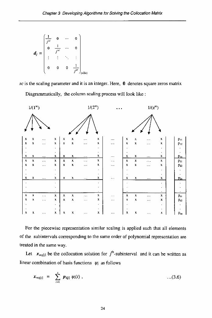
where dj are diagonal matrices of form
23
Chapter 3 Developing Algorithms for Solving the Collocation Matrix
0 0JSC0 0
dj = lC
0 0 0 le(nXn)
se is the scaling parameter and it is an integer. Here, 0 denotes square zeros matrix
Diagrammatically, the column scaling process will look like:
1/(1 SC) 1/(2SC) 1/(ZSC)
~ A\ 4\x x x x x x x x X PIIX X X X X X X X X PI2
X X X X X X X X X
X X X X X X X X X
X X X X X X X X X
X X X X X X X X X
x xx x
x x xx x x
xx
x x xx x x
x xx x
xx
PzI
Pz2
x x x PZIl
For the piecewise representation similar scaling is applied such that all elements
of the subintervals corresponding to the same order of polynomial representation are
treated in the same way.
Let xwqUl be the collocation solution for l-subinterval and it can be written as
linear combination of basis functions If/; as follows
XwqUl = :t PiU] If/i(t) ,i=1
24
... (3.6)
Chapter 3 Developing Algorithms for Solving the Collocation Matrix
where j = 1, 2, 3, ... w; w is number of subintervals and t is the independent
variable in the lh-subinterval and PiU] = [PilU] PiZU] ... PinU] ]T. Note that the
unusual notation for the additional index [j] which appears in vector PiU] is for
clarity since Pi itself is a vector.
The collocation parameter P then has the form :
P = [P1[1] PZ[I] ... Pz[l] I PI[Z) PZ[Z) .•• Pz[Z)
<:> <:>I PI[w] PZ[w) ... Pz[w)]T
corresponding to: 1st -subinterval 2nd-subinterval w'h-subinterval
Elements of the collocation matrix C associated with the elements of P will be
treated in the same ways as follows:
where i = 1,2,3, ... , z; j = 1,2,3, ... , n; k = 1,2,3, ... , w.
3.2.2 Some Results of Numerical Experiments
For illustration we employ such column scaling operation in the collocation
algorithm for solving the following boundary value problems.
Chapter 3 Developing Algorithms for Solving the Collocation Matrix
Table 3.2(Condition number & Actual Error -- Gauss Points)
-~---~--t---~~-~---------~---------------~----------------~--------------~---------------~---------8 3 I K(C) I 2.011e+08 7.775e+07 3.830e+07 3.900e+07 6.222e+07
terror t 2.2607276e-02 2.2607275e-02 2.2607276e-02 2.2607275e-02 2.2607275e-02
, I K(C) 11.68ge+08 5.602e+07 3.36ge+07 4.291e+07 6.942e+07terror t 5. 8773596e-04 5. 8773594e-04 5. 8773602e-04 5. 8773592e-04 5. 8773602e-04
5 I K(C) 12.773e+08 7.610e+07 3.887e+07 4.505e+07 7.03ge+07terror t 7.5306217e-07 7.5309675e-07 7.5299208e-07 7.5291883e-07 7.5314650e-07
8 5 I K(C) I 6.13ge+08 1.593e+08 5.512e+07 4.471e+07 6.470e+07terror t 1. 6222150e-08 1. 6039261e-08 1. 6195687e-08 1. 6138884e-08 1. 607348ge-08
This chapter is mainly concerned with numerical investigation of error estimates
for the collocation solution of linear system of differential equations. Our main
goal is to obtain a reasonable error estimate to be used directly in estimating the
number of subintervals needed in an adaptive mesh selection algorithm. Hence,
these error estimates should be inexpensive computationally and they can easily be
implemented. Some error estimates based on consideration of the linear operator
involved and on the residuals will be examined in some details.
Firstly, let us state precisely the form of problem considered and notations
used. We shall consider the linear system of n first order differential equations of
the form
x' - A(t) x(t) = yet), a < t c b ... (4.1)
where x(t) and yet) are n-dimensional vectors with components Xi(t) and Yi(t),
1::; i::; n, respectively. A(t) is an (nxn) matrix valued function.
The system of ordinary differential equations (4.1) is furnished by m and (n-m)
associated homogeneous boundary conditions at the left and right boundaries
respectively, for some positive constant m < n.
The equation (4.1) may be written in operator form
(D-M)x = y ... (4.2)
Chapter 4 Numerical Evaluation of the Error Estimates
where X E X and Y E Y in which X and Y are suitable Banach space. Here D
denoting the differentiation operator Dx(t) = dx/dt is the principal part of the
operator, and we assume that both operators D and (D - M) with the associated
conditions are invertible, Le. D-1 and (D - M)-I exist.
Suppose xwq denote the collocation solution found by collocating at q points in
each subinterval using the partition:
1tw : a = tl < ti < ts < ... < i; < tw+1 = b.
where w indicates the number of subintervals. In each subinterval [tk, tk+I],
1 :::;k :::;w, the q collocation points are uniquely determined by
tk I -tk • h . 1 2~ik = tk + + 2 (1+ ~i ) , were t = , , ... , q.
where {~;"}, 1:::; i ::;q, are the chosen reference points in interval [-1,1].
Let Xwq and Ywq be subspaces of X and Y respectively and f/Jwq is a
projection Y ~ Ywq- The approximate solution xwq taken in a subspace Xwq is
found by applying an interpolatory projection f/Jwq to the equation (4.2) with xwq
substituted for x, that is
f/Jwq(DXwq - MXwq - y) = 0 ... (4.3)
By assuming f/JwqDxwq = DXwq that is that the operator D restricted to Xwq
establishes a bijection between Xwq and Ywq so that the equation (4.3) may be
simplified as follows
f/JwqDxwq - f/JwqMxwq = f/JwqY
(f/JwqD - f/JwqM)xwq = f/JwqY
or
... (4.4)
42
Chapter 4 Numerical Evaluation of the Error Estimates
To be used in constructing the error estimate, it is convenient here to define the
compact operator K by
K = MD-I ... (4.5)
As described by Anselone in [5], the inverse of (I - K) where I the identity
operator on space X can be expressed in terms of the so called resolvent operator
(I - K)-IK as follows
(I-K)-I = I+(I-K)-I K ... (4.6)
4.2 Behaviour of the Collocation Matrix Norms
For solving single higher order differential equations, Ahmed and Wright in [2]
introduced certain matrices Qwq developed from Ahmed's thesis [1] and the
properties of those matrices were discussed in some detail. They also suggested
some efficient ways in defining and constructing such matrix Qwq. Firstly they
consider two vectors, i.e. the evaluation vector tPq: y ~ Rq to give a vector
consisting of the values of a function at the collocation points; and an additional
evaluation vector tPs: X ~ RS relating to a set of evaluation points {Si}' 1 ~ i ~ s
for some s. Secondly, for convenience they define those evaluation vectors as
Xo = tPs xwq and Yo = tPqy, both based on the collocation points. The matrix Qwq
can then be written as
xn = QwqYo ... (4.7)
that is the matrix Qwq relates the values of the right hand side and the approximate
solution at the collocation points. The equation (4.7) can be regarded as the
definition of Qwq. Under some assumptions and conditions it has been shown in [2]
that by keeping q to be fixed the norm of matrix Qwq converges to the norm of
(D - M)-I as w tends to infinity.
43
Chapter 4 Numerical Evaluation of the Error Estimates
The results presented in [2] confirm the intuitively reasonable notion that a
collocation matrix inverse can give an idea of the error magnification inherent in
the collocation process, justifying the use of IIQwq II as estimates of II (D - M)01 II.The details of matrices Qwq will not be discussed further here since our motivation
is to see the idea of using those matrices in constructing the error estimates.
For solving the first order systems of boundary value problems using global and
piecewise representation, here we have carried out further work on observing the
convergence of IIQwq II based on numerical investigations. The usefulness of
IIQwq II as estimates of II (D - M)0111 is observed. Moreover, in some cases the
IIQwq II may settle down early. Briefly, the numerical results which are not
presented here indicate that
and
IIQwq II ~ II (D - M)0111 ' as q ~ 00, w fixed
However, since the evaluation of IIQwq II involves the inversion of a large
matrix generated by the collocation process, certainly it is a massive computational
task and the estimate is very expensive. This in tum suggests that one would expect
considerable cancellation in using this estimate for adaptive mesh selection
algorithms.
4.3 The Res id u a I
Having carried out the collocation process, suppose an approximate solution Xwq
satisfying the differential equation (4.1) and its associated boundary conditions has
been found. The residual of the approximate solution xwq denoted by r wq is
defined as
rwq = (D -M)xwq - Y '0.(4.8)
44
Chapter 4 Numerical Evaluation of the Error Estimates
Using the following simple algebraic manipulation and applying the equation
(4.4) we have relationship
rwq = (D - M + f/JwqM - f/JwqM )xwq - y
= (D - f/JwqM)xwq - MXwq + f/JwqMxwq - y
= f/JwqY - Y + f/JwqMXwq - MXwq
= (f/Jwq - I)y + (f/Jwq -I)Mxwq
= (f/Jwq -1)(Mxwq +y) ... (4.9)
From the equation (4.9), it is clear that the residual rwq is the error in the
interpolation of the function (Mxwq + y), hence this enables us to examine its
behaviour using some properties of the interpolation theory.
The Cauchy remainder theorem for polynomial interpolation described in detail
in Davis [20] states that in interpolating a continuous function fit) over the closed
interval [a,b] based on (n+1) interpolation points: a :5 to < tl < ... < t« :5 b
providing r=» exists at each point of (a.b), the remainder RnCt) then satisfies
where the point ~ depend upon t, to, tl, ... , tn and function fAs we can see from the Cauchy theorem, the remainder RnCt) splits into two
nparts. The first part, the factor (n~l) IT (t - ti) , is independent of function fit), but
i=O
depends upon the interpolation points. The second part, jn+I)(?>, depends upon
function interpolated, but is independent of the manner in which the interpolation is
carried out. The second part tells us that the remainder RnCt) is affected by the
smoothness of fit).
Looking at the function CMxwq + y), if we assume that the coefficient ACt) in
differential equation (4.1) is sufficiently smooth and using the fact that xwq itself is
a piecewise polynomial function and if yet) is assumed to be smooth enough as
45
Chapter 4 Numerical Evaluation of the Error Estimates
well, then r wq should be well approximated by a piecewise polynomial found by
interpolation using additional points in each subinterval. Furthermore the residual
rwq will have a factor
in the kth-subintervals.
This suggests that the residual may split into two parts, the first part called the
principal part of the residual consists of a polynomial which is interpolating the
residual; the second part is the error in the interpolation. Let r;q denotes the
principal part of the residual rwq and r;; denotes the error term in the interpolation
we then have
From this point, there are several ways to construct a polynomial interpolation
for the principal part of residual r;q. At least there are two considerations which
should be taken into account in constructing such a polynomial. Firstly, we wish
that the integration process of the chosen polynomial interpolation can be carried
out in a simple way, since we need to carry out the integrations to form D-1 r;q(discussed in the following section). Secondly, the polynomial interpolation should
be sufficiently accurate even for the cases where the number of interpolation points
is small. For the first consideration, it is convenient to represent r;q as a
Chebyshev series since the integration process can be carried out easily. The
second consideration relates to the way of choosing the interpolation points. Here,
since the residual is zero at the collocation points, one might consider to choose
points between the collocation points, so as to get close to the extrema of the
residual. If the end points of the subintervals are not the collocation points, one
46
Chapter 4 Numerical Evaluation of the Error Estimates
might also consider to take them as additional interpolation points. Based on those
considerations, it is convenient to use (2q+1) interpolation points determined by
t, = cos(~-~1£), i = 1, 2, ... ,(2q+l); q is the number of collocation
points, and then express r;q as
• *rwq (t ) 2q *= I Cj 1)(t ),j=O
... (4.10)
where 1)(t*) are Chebyshev polynomials and t* denotes a local variable in each
subinterval.
To examine how well the polynomial interpolation based on equation (4.10)
performs in computation, we observe some results of numerical experiments using
a number of problems having different nature.
In tables (4.1), (4.2) and (4.3) the capital letters R, R*, R** denote values of the
norms, i.e. R = Ilrll, R* = II r;q II, R** = II r;; II; the letters C and G standing for
Chebyshev and Gauss indicate whether Chebyshev zeros or Gauss points have been
used as the collocation points. As usual, q and w indicate the number of
collocation points and the number of subintervals respectively.
For the first illustration, let us consider the following problem
Example 1 :
constrained by the boundary conditions
x1(-1) = e-1 + 1. x2(-1) = e-1 - 3;
x1(2)= e2_8
47
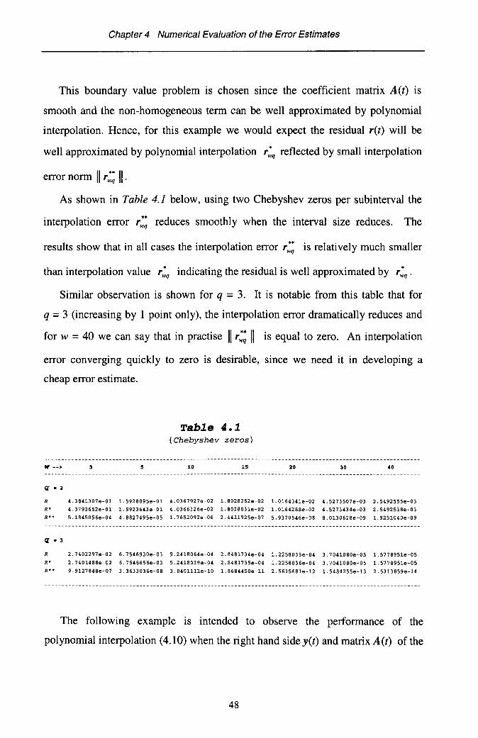
Chapter 4 Numerical Evaluation of the Error Estimates
This boundary value problem is chosen since the coefficient matrix A(t) is
smooth and the non-homogeneous term can be well approximated by polynomial
interpolation. Hence, for this example we would expect the residual ret) will be
well approximated by polynomial interpolation r:q reflected by small interpolation
error norm II -: II.
As shown in Table 4.1 below, using two Chebyshev zeros per subinterval the
interpolation error r:; reduces smoothly when the interval size reduces. The
results show that in all cases the interpolation error r:; is relatively much smaller
than interpolation value r:q indicating the residual is well approximated by r:q.Similar observation is shown for q = 3. It is notable from this table that for
q = 3 (increasing by 1 point only), the interpolation error dramatically reduces and
for w = 40 we can say that in practise II r:; II is equal to zero. An interpolation
error converging quickly to zero is desirable, since we need it in developing a
Chapter 4 Numerical Evaluation of the Error Estimates
4.6 Numerical Evaluation of the estimate E* for Stiff' BVPs
Although here the concept of stiffness for system of differential equations will
not be discussed in detail, in this section using numerical experiments we shall
observe performance of the error estimate E* when dealing with stiff problems
having severe layers.
Firstly let us consider the following problem
Problem 6:
(;:) = (: ~)(;:)+LcOS'(,")+~'COS(2mJThe boundary conditions and the analytical solutions are given by
XI(O) = xl(l) = 0
This is a 'real' problem and one reason for choosing this problem is that it has
been used elsewhere to show that some procedures do not perform well [19]. In
this problem, since the solution X2 behaves badly, i.e. it undergoes a drop from
X2 = ~Jl to X2 = 0 within small subinterval [0,. II'JJl] and near the right end it
rises from X2 = 0 to X2 = ~Jl within subinterval [~I , 1], we may expect that
the errors in calculating X2 should be worse compared to those in calculating XI.
Moreover, even though the non-homogeneous term of this problem is not a
polynomial it can be well approximated by a polynomial, hence the residual will
be well approximated by r;q in which the interpolation error r;; will be very
close to zero, hence we would expect that the cheaper estimates E* can be used
instead of the estimates E2 and E3•
Using the Gauss points, Table 4.9A and Table 4.9B contain results with
problem parameter Jl = 102 and Jl = 104 respectively.
66
Chapter 4 Numerical Evaluation of the Error Estimates
In Table 4.9A it is observed that the estimate E* is reasonably satisfactory even
if the approximate solution is poor. The estimate improves as the number of points
q increases as well as the interval sizes decrease. Looking at q = 2 and w = 3,
since IID-l r;q II is much smaller than IIKr;q II it is clear that large IIKr;q II resultsin a poor error estimate. Comparing the norms IIr II and IIrh II it is again very
clear that IIrh II provides a better approximation.
With problem parameter Jl = 104 the problem is set to have more severe layers.
As can be seen in Table 4.9B, this implies that 11K r;q II become even larger and in
all cases IIK r;q II is much larger than liD-I r;q II. It is clear that 11K r;q II is the
*dominant term in the equation forming E. From this table, it is notable that if the
solution is very poor then the estimate will also be very poor. With this important
note, we realise that the estimate may perform very poorly at initial stages of a
mesh selection algorithm.
q w
2 32 52 102 202 402 50
3 33 53 103 203 403 50
5 35 55 105 205 405 50
Table 4.9A(Gauss Points, problem parameter ~ = 102)
At some stage of the piecewise polynomial collocation methods for solving
boundary value problems, discretisation of the differential equations on a mesh is
involved. The purpose of this chapter is to study the practical selection of such a
mesh, with the objective of achieving a sufficiently accurate solution as cheaply as
possible.
We will start by introducing some basic concepts. For comparison purposes, it
will then be followed by reconsidering some well known mesh selection algorithms.
Subsequently, we will introduce and discuss a proposed criterion function to be used
in adaptive mesh selection algorithms. Finally some results of numerical
comparisons are presented.
The basic problem considered is the two-point boundary value problem
x'(t) = A(t) x(t) + y(t), a <t< b ... (5.la)
... (5.lb)
Here we assume that there is an unique solution x(t) that we wish to compute and
that matrix valued function A(t) is sufficiently smooth.
In the collocation process using q collocation points per subinterval, the
discretisation of the differential equations will be carried out on the mesh
1t : a = tl < ti < ... < tw < tw+1= b ... (5.2)
Chapter 5 Adaptive Mesh Selection Algorithms
where w denotes number of initial subintervals.
The mesh sizes are defined as hi = ti+l - t, , 1 ~ i ~ wand the maximum mesh size
is h = max hi. For convenience, the resulting collocation solution on the mesh 1ti
will be denoted by x1t(t) rather than Xwq(t) as in previous chapters.
Since we shall be interested mainly in developing our proposed criterion function
and examining its performance by carrying out numerical comparisons with those
well known mesh selection strategies, here the problem of selecting a good mesh is
considered independently from error estimates. To be precise, in the numerical
experiments we shall directly examine and compare the performance of algorithms
by looking at the actual error at certain number of collocation points w.
For simplicity and to make numerical comparisons more straightforward and
more clear, in implementing the adaptive mesh selection algorithms to be presented
here the number of subintervals will be incremented by one subinterval per iteration.
This means that neither the possibility of adding a number of knots nor reducing the
number of knots will be pursued here, however it will be considered in the next
chapter.
5.2 Some Basic Concepts
In the three following subsections some basic concepts underlying our work will
be introduced.
5.2.1 Structure of Adaptive Mesh Selection Algorithms
The idea of adaptive refinement of a mesh and a redistribution of meshes are now
well established. A number of robust mesh selection algorithms are available and
have been applied widely in developing many software packages.
There is not much theoretical justification for the different strategies which have
been used widely. Even though some strategies based upon asymptotic formulas
perform quite satisfactorily in many practical applications, despite this lack of
rigorous theoretical justification. It is important to realise that in the development of
71
Chapter 5 Adaptive Mesh Selection Algorithms
mesh selection algorithms that the choice of a good mesh is not very sensitive; i.e.
often there is a wide range of acceptable meshes of a given size w for a given
boundary value problem, even when a uniform mesh of the same size yields poor
results.
In developing mesh selection strategy, the aim is to find an algorithm which
determines a sequence of partitions defined by the points (knots) in an adaptive way,
so that an accurate solution to the problem is obtained with as small number of
subintervals w as possible.
To be more precise, let TOL be the desired tolerance, and suppose we wish to
compute the approximate collocation solution x1t(t) of BVP (5.1) over partition (5.2)
using q collocation point per subinterval. Having computed x1t(t) on mesh n, our
main goal is to efficiently determine a new partition of [a, b]
*n ... '" '" lie ba = tl < t2 < ... < two < twO+1 = ... (5.3)
such that w* is small but if the collocation solution is computed using n* then the
global error e(t) satisfies
II ell == max II e(t) II s TOLas/Sb
... (5.4)
Needless to say that the mesh (5.3) and collocation solution may need to be
repeatedly updated until (5.4) is satisfied.
It is clear that some criterion function Ti(t) is needed to construct a new mesh n*.
Basically, there are two approaches to do this, firstly by trying to redistribute Ti(t)
which should be some measure of the error in the ith-subinterval, such that they have
approximately the same norm in whole range [a, b], i.e. by requiring
IITi II = constant = F;, 1$ i$ w ... (5.5)
secondly, we directly attempt to minimise Ti(t) simply by searching for the
subinterval(s) having large IITi II and then subdivide these subintervals.
72
Chapter 5 Adaptive Mesh Selection Algorithms
Having chosen a particular criterion function, an adaptive mesh selection
algorithm can be constructed by means of an iterative procedure, adding or removing
points as necessary to equilibrate to level E. An approximately equilibrating mesh is
produced such that the equation (5.4) is fulfilled.
An outline of basic structure of the procedure is as follows
o
1. Compute the first stage collocation solution on initial mesh n
2. Evaluate the global error and check whether either
(5.4) is satisfied ornumber of iterations exceed some prescribed constant Imax or
number of subintervals greater than some constant wmax
~ and then break
3. Evaluate the criterion function
4. Construct a new partition n· based on result of step-3
o
o
5. Compute the collocation solution on new mesh n·
6. Repeat step-2
5.2.2 Error Equidistribution and Criterion Function
A particular approach to adaptive collocation schemes was introduced by
de Boor [22]. In the paper, de Boor proposed to equidistribute some certain measure
of the error in each subinterval [ti, ti+d. Furthermore, a paper of Pereyra and
Sewell [40] discusses in some detail the concept of equidistribution for discrete
solutions. In the paper they extend the idea of de Boor to discrete variable
approximation for more general for boundary value problems.
Recall 'Zl the local error measure mentioned in the previous section. The
requirement using equation (5.5) may be regarded as the basic definition of the
equidistribution concept. However, as described in Ascher et al. [10], since this
error measure is not independent of its associated subinterval [ti, ti+1] and in
general 'Zl increases as the mesh size increases, it will tum out to be convenient to
73
Chapter 5 Adaptive Mesh Selection Algorithms
consider a corresponding error measure fA which only varies linearly with hi , Le.
they are related by
... (5.6)
where T, is independent of mesh size hi.
Having chosen a suitable criterion function 11 (or perhaps, the converted one of
the form (5.6)) the new mesh n· may be found by requiring max II fA II to bel$i$w
minimised. This brings us to the minimax problem with one constraint as follows
find the set of points {I;, I;, ... , I:.} c (a, b) such that
max II t, II (/;+1 - I;) is minimum,l$i$w·
where (/;+1 - t;) > 0 and the sum of (t;+1 - t;) must satisfy
•w,,* *~ (ti+l-ti) = (b-a).i=l
The above optimisation problem can be solved, simply by making all f/J; = T, hi
equal to the same constant E. This result enables us to define formally the concept
of equidistribution as follows
Definition: A mesh points is said to be equidistributing with respect to the function
T(t) if and only if
II T(t) II i hi = constant, i = 1,2, ... , w ... (5.7)
For the sake of generality, especially to understand what has been done by de
Boor, we can extend the definition (5.7) by considering a more general function p (t),
instead of just discrete values function II T(t) II i on partition rt. Let us assume that
a positive valued function At) is continuous and sufficiently smooth. With these
assumptions, we come to the following definition.
74
Chapter 5 Adaptive Mesh Selection Algorithms
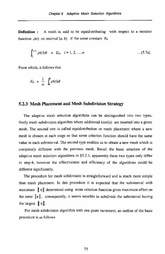
Definition: A mesh is said to be equidistributing with respect to a monitor
function !Xt) on interval [a, b] if for some constant Eo
(+1J,' p(t)dt = Eo,, i = 1,2, ... ,W ... (5.7a)
From which, it follows that
Eo = ~ f p(t)dt
5.2.3 Mesh Placement and Mesh Subdivision Strategy
The adaptive mesh selection algorithms can be distinguished into two types,
firstly mesh subdivision algorithm where additional knot(s) are inserted into a given
mesh. The second one is called equidistribution or mesh placement where a new
mesh is chosen at each stage so that some criterion function should have the same
value in each subinterval. The second type enables us to obtain a new mesh which is
completely different with the previous mesh. Recall the basic structure of the
adaptive mesh selection algorithms in §5.2.1, apparently these two types only differ
in step-4, however the effectiveness and efficiency of the algorithms could be
different significantly.
The procedure for mesh subdivision is straightforward and is much more simple
than mesh placement. In this procedure it is expected that the subinterval with
maximum II 1; II determined using some criterion function gives maximum effect on
the error IIell, consequently, it seems sensible to subdivide the subinterval having
the largest II 1; II·For mesh subdivision algorithm with one point increment, an outline of the basic
procedure is as follows
75
Chapter 5 Adaptive Mesh Selection Algorithms
or w > wm••' for some constant wm••
1. Solve the BVPusing a crude initial mesh points
2. Evaluate the criterion IltJ, i = 1,2, ... , W
3. Searching for the subinterval which has maximum IItJ4. Halve this subinterval5. Repeat first step till either (5.4) is satisfied
Note that, the basic procedure above can be developed further to obtain an adaptive
mesh algorithm with multiple subdivisions.
For mesh placement algorithms, a special procedure is needed which involves
setting up and finding the inverse of a certain function. A detailed description on this
can be found in §5.4.2.
5.3 Some Well Known Criterion Functions
In the following subsections, we shall examine some well known criterion
functions widely used in applications. Our main attention is the maximum residual
and de Boor criterion functions which will be employed for numerical comparisons.
Some other criteria will be described briefly.
5.3.1 Maximum Residual
Residuals have been commonly used to estimate the local errors for mesh
selection. Carey and Humphrey [14] studied in detail the use of residual as criterion
function in developing adaptive mesh selection algorithms. In their work they also
found some empirical relations for some specific problems for which they come to
conclusion that reducing the residuals in some region will reduce the residual in
whole interval and consequently, the global error. This result is also pointed out in
Seleman's thesis [48].
76
Chapter 5 Adaptive Mesh Selection Algorithms
To recall, for a given mesh 1t of (5.2) and q given collocation points in each
subinterval, the residual r1t(t) for the boundary value problem (5.la-5.1b) is
determined by
rit) = (D - A) xit) - yet) ... (5.8)
where D denotes the differential operator defined in chapter 2.
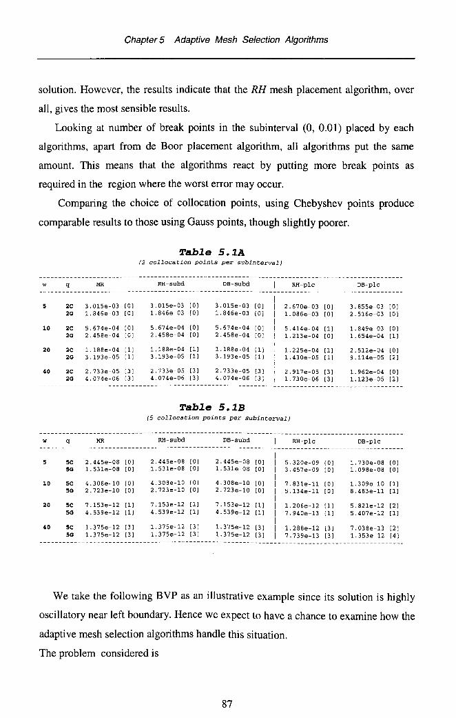
Implementing this strategy which will be called the MR strategy is fairly simple.
The main task is to search for the subinterval having the largest residual and then
subdivide the subinterval into two equal subintervals. As we can see in
equation (5.8), the residual can be evaluated at any point straightforwardly,
nevertheless obtaining its maximum is not a cheap computation task, especially if the
mesh is a non-uniform one. Obviously, the success of a maximum residual strategy
also depends on the success of estimating the largest residual. There are various ways
that an approximate residual can be found and used for this purpose, here we will
make use the polynomial interpolation discussed in chapter 4 to obtain an estimate
of maximum residual.
5.3.2 De Boor's Algorithm
De Boor's paper of 1973 [22] is recognised as one of the most outstanding
contribution in developing adaptive mesh selection algorithms. De Boor introduced
a criterion function based on the error analysis given in de Boor and Swartz's
paper [23]. A comprehensive paper of Russell and Christiansen [45] discusses
further de Boor's idea, and this is implemented in the COLSYS code by Ascher,
Christiansen and Russell as described in Ascher et al. [IO].
For comparison purposes, first of all we shall take a look at de Boor's idea in
constructing an adaptive mesh placement algorithm.
Let us start by reconsidering some theoretical results about collocation
approximation method and its error estimates which can be found in [22,45].
77
Chapter 5 Adaptive Mesh Selection Algorithms
For t E (ti, ti+1) , under certain conditions it is known that for some integer d > q
the global error e(t) satisfies the local inequality
... (5.9)
and
IIx1t(t) - x(t) II i :5 O(hd), 1:5 i:5 w+1
where hi, h denote the interval sizes and C is a constant determined by
1 r qC = 1 max {l IT(s - qj )ds}
2q+ q! -rs.sr 1 j=l... (5.10)
where Q are the collocation points in [-1,1]
It is also shown that closer examination of the error reveals that (5.9) can be
replaced by the equality
... (5.11)
This implies that, for sufficiently small h
... (5.12)
and therefore suggest that break points tz. ts, ... , t; be placed so as to minimise the
maximum of local terms hjq+11Ix(q+1) (t) II j. This can be achieved by requiring
hjq+1 Ilx(q+I)(t) II i = constant, i = 1,2, ... ,W ... (5.13)
Based on (5.13) de Boor constructed an adaptive mesh selection procedure which
produces a complete new mesh in each iteration, in other words it is a mesh
placement algorithm. Due to unavailability of X(q+1)(t), and since X1t(q+1)(t) is zero
within each subinterval, de Boor proposed a numerical scheme to obtain an
approximate for the terms IIx(q+l)(t) II j using values in neighbouring subintervals.
The piecewise constant function to approximate X(q+1) (t) is determined using
78
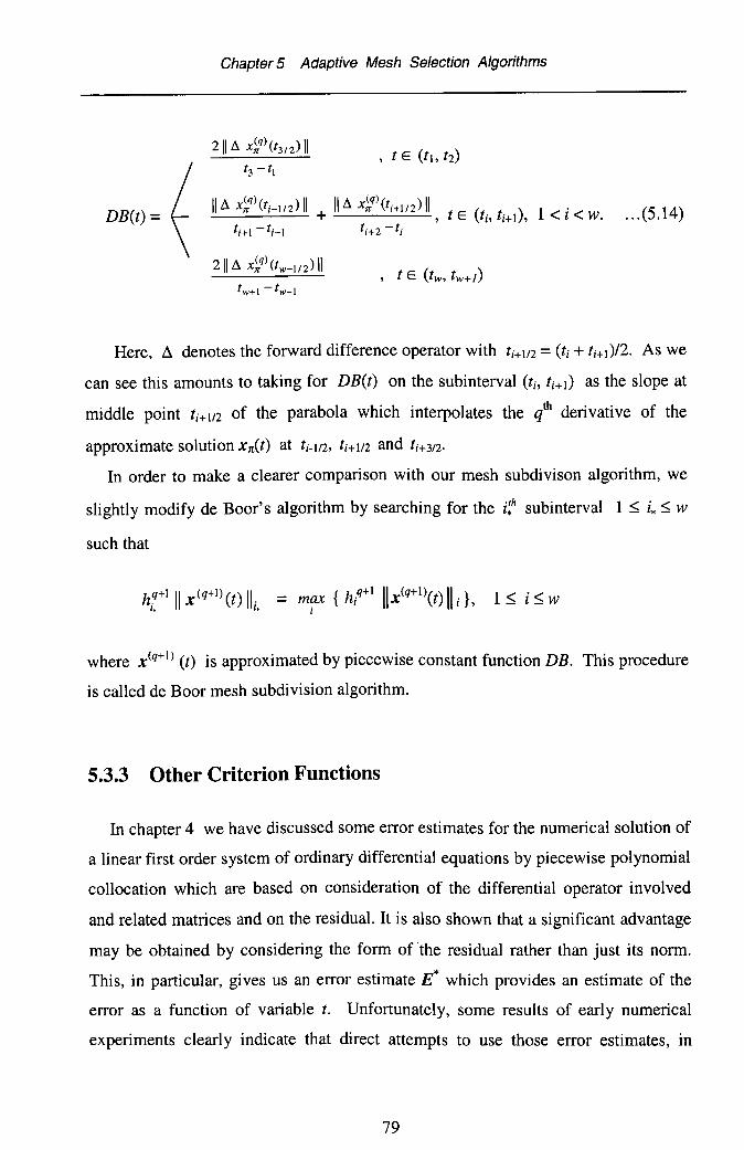
Chapter 5 Adaptive Mesh Selection Algorithms
211 ~ x~q)(t3l2) IIt3 - t1
DB(t) = ... (5.14)
Here, fj. denotes the forward difference operator with ti+1I2= (ti + ti+I)/2. As we
can see this amounts to taking for DB(t) on the subinterval (ti' ti+l) as the slope at
middle point tusn of the parabola which interpolates the qth derivative of the
approximate solution x1t(t) at ti-1I2, ti+1I2 and ti+312.
In order to make a clearer comparison with our mesh subdivison algorithm, we
slightly modify de Boor's algorithm by searching for the i!h subinterval 1:::; i.:::; w
such that
htl II X(q+l) (t) IIi. = max { hiq+1 Ilx(q+I)(t) IId, 1:::; i:::; w
I
where X(q+l) (t) is approximated by piecewise constant function DB. This procedure
is called de Boor mesh subdivision algorithm.
5.3.3 Other Criterion Functions
In chapter 4 we have discussed some error estimates for the numerical solution of
a linear first order system of ordinary differential equations by piecewise polynomial
collocation which are based on consideration of the differential operator involved
and related matrices and on the residual. It is also shown that a significant advantage
may be obtained by considering the form of the residual rather than just its norm.
This, in particular, gives us an error estimate E* which provides an estimate of the
error as a function of variable t. Unfortunately, some results of early numerical
experiments clearly indicate that direct attempts to use those error estimates, in
79
Chapter 5 Adaptive Mesh Selection Algorithms
particular E*, as criterion function in developing an adaptive mesh selection
algorithm for solving system BPVs give unsatisfactory results. Though, Wright,
Ahmed and Seleman [60] have shown that if the influence of the behaviour in one
subinterval on the error in others is taken into account then some criterion functions
based on those error estimates for solving single higher order boundary value
problems may give a good results in some cases. These modified criteria tum out,
however, to be very expensive and their practical utility is doubtful.
For solving single higher order boundary value problems, there have been many
suggestions for criteria. Some of these aim to reflect some measure of smoothness of
the approximate solution, for example the magnitude of a particular derivative of the
collocation solution in each subinterval. For this purpose, White [53] suggested the
use of arc-length, while Dodson [24] proposed to approximate the particular
derivative by differentiating the piecewise linear function that interpolates the
derivative at the middle of subintervals. Other criterion functions relate to some
measure of error. These criterion functions, however, will not be considered further
here except to remark that the de Boor algorithm which involves approximating the
particular derivative of xit) is widely used and performs quite well as pointed out by
Russell and Christiansen [45]
5.4 Using rh, as the Criterion Function
In this section, a criterion function to be used in developing adaptive mesh
selection algorithm will be introduced. Firstly we consider some motivation for
choosing this criterion and then it is followed by developing a numerical scheme for
mesh placement algorithm based on our criterion function.
5.4.1 Motivation for Using rh, as the Criterion Function
The standard analysis of collocation process for solving the boundary value
problem (5.la-5.lb) using q points per subinterval over mesh points (5.2), yields the
error e(t) which can be expressed as
80
Chapter 5 Adaptive Mesh Selection Algorithms
e(t) = f f+1 G(t,s)r(s)ds;=1 I
... (5.15)
where res) is the residual defined in equation (5.8) and G(t,s) denotes the Green's
function. For t E (ti' ti+l) let us consider the terms
ej(t) = rG(t,s)r(s)ds, i = 1,2, ... , w.I
.. .(5.16)
It is notable that firstly the residual res) is local in nature and has been used as
criterion function in adaptive mesh selection algorithm [10,14,59], secondly
regarding the relationship between the global error and local terms Russell and
Christiansen [45] have pointed out that the global error is asymptotically dominated
by local term when Gauss points are used. Lastly, in applications usually the Green
matrix function is diagonally dominant [29,31]. These results suggest that ei(t) in
equation (5.16) is dominated by the residual res) and G(t,s) may be taken to be
constant for t E (ti' ti+l) , S E (ti' ti+l) and zero elsewhere, we then have the local
term
Ilei(t) II = II c t+1 r(s)ds II s C f+1Ilr(s)lIds = Cllrlli hi
I I
... (5.17)
For some constant C. hi, as usual, denotes the mesh size of ith -subinterval.
Since the equation (5.17) reflects some measurement of the error and is local in
nature, it seems reasonable to take it as a criterion for an adaptive mesh selection
algorithm which will be called RH mesh selection algorithm.
Furthermore, taking equation (5.17) as criterion is also suggested by the following
results. Suppose the collocation points are the zeros of certain orthogonal polynomial
and we take the number of collocation points q to be even, i.e. the ODE (5.1a) will
not be collocated at the middle of subintervals. Using the fact that the residual ret) is
zero at the collocation points Qj, it has been shown in [45] that in each subinterval
the residual satisfies
81
Chapter 5 Adaptive Mesh Selection Algorithms
... (5.18)
Since the middle of subinterval is not the collocation point solving (5.18) for X(q+l)
in term of r(ti+ll2) gives
(q+I)( )X ti+1I2 =
By taking the norm of the last equation and substituting into (5.11) we then have
an error estimate
... (5.19)
This suggests, corresponding to the discussion in §5.2.2, that trying to
equidistribute the equation (5.19) introduce a mesh selection algorithm with respect
to the function T(t) (see equation (5.6»
II T(t) II i == II r(ti+1I2) II '
hence equation (5.17) can be regarded as the general form of equation (5.19).
It is notable that in computing the error estimate E*, we have to evaluate residuals
and construct an approximate residual r*(t). This, in tum, makes the application of
criterion rh, more convenient and less expensive if we develop an adaptive mesh
selection algorithm while also using the error estimate E*, since we can make use
the computed r *(t) for approximating the local terms II r(t) II i » It is also notable that
the RH algorithm is as cheap as the MR algorithm since the main cost is to evaluate
the residual in each subinterval.
5.4.2 Developing the Scheme for Equidistributing the Terms rh,
We will now employ the equation (5.17) in constructing two adaptive mesh
selection algorithms, i.e. RH mesh subdivision and RH mesh placement algorithms.
82
Chapter 5 Adaptive Mesh Selection Algorithms
The RH mesh subdivision algorithm is quite simple in implementation, where the
main task consists of searching for the subinterval which has maximum II r(t) II i hi,and then subdividing this subinterval into two equal subintervals.
Unlike the RH mesh subdivision algorithm, the RH mesh placement algorithm
needs a special scheme to equdistribute the local terms II r(t) II i hi which will be
developed in this section.
The residual r(t) can be related to mesh size hi by equation
... (5.20)
for some positive constant k, and some constant integer s.
Multiplying both sides by hi we have
... (5.21)
Therefore, equidistributing the local terms in (5.17) is equivalent to equidistributing
the local terms kihrl.
Having computed rn on the initial mesh n, a new partition n* of the form (5.3)
producing a more accurate solution is desired.
Supposed that the width of ith-subinterval in new mesh n* is denoted by
* * *h i = (t i+1 - t D. To equidistribute (5.21), it requires
k1h1*s+1 - k h*s+1 - - k h*s+1- 22 -···-ww
to give
(h~ / h;) = (k2 / k1)1/(s+1)
o; /hi) = (k3 / k1 )lI(s+ 1)
83
Chapter 5 Adaptive Mesh Selection Algorithms
By taking (k, / kl)lI(s+l), 1 ~ i ~ w, as the slopes of a piecewise linear function
with the slope in the first subinterval is set to be one, we can then construct a
piecewise linear function fJ.,t) as follows
fJ.,t) ::: ... (5.22)
where ki::: Ilrll J ht , i::: 1,2, ... ,w.
Here we approximate ret) using the principal part of the residual (described in
chapter 4) formed by evaluation at a suitable set of Chebyshev extrema.
Since fJ.,t) is a continuous and monotone increasing piecewise linear function,
we can then easily compute e-I(t) and evaluate it at the (w *+1) points
((i-I) e(b) / w\ 1s i s (w*+1)
giving us a new mesh n*.
For illustration, suppose the current number of subintervals w ::: 4 and it is
increased by one subinterval in the next stage, i.e. w * ::: 5. Using the approximate
residual /(t) we then construct the piecewise linear function e(t). The new mesh n*
having break points {t*;}, 1~ i ~ (w*+l), is determined as follows
* ::: e-I(O) . * e-I( 8(b) )t I ::: a t 2 :::w*
* e-I( 2 8;b) ). * e' 3 8(b)t 3 ::: t 4 ::: (~)W
* e-I( 4 8;b) ). * b ::: e-I(fJ.,b»t 5 ::: t 6 :::w
A graphical illustration of the process is shown by the graph on the following page
84
Chapter 5 Adaptive Mesh Selection Algorithms
...---- B(t)
5.5 Numerical Results
o
Several numerical experiments were performed with the adaptive mesh selection
algorithms described in the previous sections. In order to give an impression of the
performance of the algorithms we consider some examples having various features.
These include some problems having either interior or boundary layers as well as
problems with a singularity at an end point.
In the tables below displaying some results of numerical experiments, MR stands
for maximum residual indicating the maximum residual is used as the criterion
function. RH and DB indicate max RH and de Boor algorithms respectively, while
subd and pic stand for subdivision and placement algorithm. The integer in the square
bracket [...] shows the number of subintervals in the layer regions. The last
abbreviations the capital letters C and G indicate that Chebyshev and Gauss points
are used in the numerical experiments.
85
Chapter 5 Adaptive Mesh Selection Algorithms
In all computations, we start with four-equal subintervals and then increase the
number of subintervals w by one. At certain w, we retrieve the actual error to be
displayed in the tables.
As the first example we consider the following problem
Problem 1 :
furnished by boundary conditions
X2(0) = ° and xl(l) = 5.5
The analytical solution is given by
(Xl) ( -t + _~S-"-sii~--:-~("':-:(~~i JX2
= lOt cosh(2t) - 5sinh(2t)
t2 sinh(2)
This boundary value problem is taken from Russell and Shampine [47] in which
they discuss some collocation methods for dealing with singular boundary value
problems. The problem has a singularity at t = 0, but only in the coefficient and its
solution is smooth. In their paper, it is also shown that numerically the maximum
error always occurred at the left boundary. In this example, it is expected that the
adaptive mesh selection algorithms should concentrate break points near left
boundary.
Tables S.lA and S.lB contain the results obtained by using two and five
collocation points per subinterval respectively. By looking at the actual error, it is
clear that all strategies perform quite well. In both tables we can see that the accuracy
improves smoothly as the number of subinterval increases indicating the
convergence of the collocation solution.
It is interesting to note that for the subdivision strategies, all criterion functions
used produce identical results, this means if we use subdivision strategy for this
problem the cheapest criteria MR may be adequate to obtain a sufficiently accurate
86
Chapter 5 Adaptive Mesh Selection Algorithms
solution. However, the results indicate that the RH mesh placement algorithm, over
all, gives the most sensible results.
Looking at number of break points in the subinterval (0, 0.01) placed by each
algorithms, apart from de Boor placement algorithm, all algorithms put the same
amount. This means that the algorithms react by putting more break points as
required in the region where the worst errormay occur.
Comparing the choice of collocation points, using Chebyshev points produce
comparable results to those using Gauss points, though slightly poorer.
Table 5.IA(2 collocation points per subinterval)
w q MR RH-subd DB-subd I RH-plc DB-plc------------------- ----------------------------------------------------------- -----------------
IS 2C 3.015e-03 [OJ 3.015e-03 [OJ 3.015e-03 [OJ I 2.670e-03 [OJ 3.S55e-03 [OJ
and produces therefore asymptotically the same distribution of t; 's as the problem of
determini {* * *} hetermining t2, t3, ••• , tw* so t at
w(C ki )lI(s+ 1) h;_* = -;.. I (C ki )1I(s+ 1) h;_*
w i=1
since k, are constant values, the above can be written as
t+l(Cki)1/(S+1)dt =I
... (6.9)
where k(t) is a piecewise constant function, i.e. k(t) = k;, t E (t;, t;+l)
Using (6.8) and (6.9) we have
~C1l(s+1) t k1/(s+1)dt = (TOL)1I(s+1)w
or
+w =
f k1l(s+ 1)dt
(TOL)1I(s+ 1)C
... (6.10)
99
Chapter 6 Predicting the Number of Subintervals Needed in the Collocation Process
Our developed numerical scheme to determine the break points {t;, t;, ... , t:.}
using criterion function rh, does not have the form 1kl/(s+l)dt, hence we slightly
modify the equation (6.9) by multiplying both sides with factor dc}J(S+l) to give
I _1_C1/(s+1) ~ kll(s+l)dt =(A;F(s+l) w* .b
I
I (TOL)7+i(A;F(s+l)
-;'Cll(S+I) l(kl kl)l/(s+l)dt =w
or
*w =f (k I kl )lI(s+ I) dt
(TOLl Ckl)lI(s+l)
The estimate w *, therefore, can be written
... (6.11)
here the notation r ...1 indicates the smallest integer greater than expression.
With a given TOL, w * can be calculated easily since ~ is the value of the piecewise
constant function at the right boundary described in §5.4, ki = II r II i I h/ , while C is a
constant estimated using the algorithm on the following section.
Let w; denotes the estimate of number of subintervals needed in i1h-subinterval for
the next iteration. This estimate will be proportional to r (k I kl )lI(s+ I)dt , and can be,
determined
ClI(s+l) f+l (k I kl)lI(s+l) dtI
Cl/(s+ I) f (k I kl )lI(s+ I) dt*W
to give
w; = I(T~L)I/(S+I) f+l (k)lI(s+l) dt l, 1 s i ~w ... (6.12)
100
Chapter 6 Predicting the Number of Subintervals Needed in the Collocation Process
6.3 Estimating the Constant C
Let the error estimate for the current iteration E* be found using the formulae
described in chapter 4. It has been shown that for problems having sufficiently smooth
solution and the matrix coefficient is not very large the error estimate E* is a very
reliable estimate even if the approximate solution is very poor. The basic idea here is to
employ the estimate E* in predicting the constant C in equation (6.7).
Since the residual res) is zero at the collocation points, it can be written in form
... (6.13)
By considering the local terms e. , 1 ~ i ~ W, as in equation (6.3) and then using
(6.13) and the properties of the Green's function, it has been shown in [23] that the
global error e(t) = x(t) - xwq(t) satisfies the local terms:
... (6.14)
where x(t) and xwq(t) are the exact and the approximate solution respectively, and the
constant C shown in the appendix part of [45] is dependent only on the number of
collocation points q, and satisfies
q
C = \ max {~ IT (s - ~j )ds}, ~ the collocation points in [-1,1]2q+ q! -1~t~1 11 j=t
Furthermore, Russell and Christiansen [45] have also shown that the residual ret) and
exact solution x(t) are related by
Using equations (6.7) and (6.14), the RH algorithm may be regarded as an adaptive
mesh algorithm trying to equidistribute the local terms in equation (6.5).
Hence, using equation (6.6) we then have
max {C IIr IIi hj} = max { C k, h;'+l } =i I
max IlelljI
1s t ~W
this immediately gives an estimation for C
101
Chapter 6 Predicting the Number of Subintervals Needed in the Collocation Process
c: = E* / (max {II r IIi hd)i
... (6.15)
It is also worthwhile to note here that for some boundary value problems having
severe layers the estimate E* is unsatisfactory if the approximate solution is very poor,
in particular it is larger than the actual error. As the result, the estimate C*might be very
large. This clearly indicates that the estimate w * should be used carefully, especially in
the initial stages of the collocation process, where the approximation may be very poor.
6.4 Practical Implementation
As mentioned in the previous section the approximation w;' might be very poor in
the first iterations of the collocation process, especially when the initial mesh points are
very crude and the problems have severe layers. From this point of view, it is
unreasonable to apply the estimate w * into algorithm without any additional restrictions
in the first few iterations. Hence, to implement a practical mesh selection strategy,
additional modifications are needed to ensure that the strategy does not go awry.
Firstly we note that it seems sensible to restrict the size of w * particularly in the first
few iterations. Some simple techniques widely used in mesh adaptive algorithms, for
example doubling the number of subintervals, immediately give us an obvious choice of
such restriction, i.e. w * should be taken no more than doubling the current number of
subintervals w. Furthermore, we may utilise some values arising in the computation
process, for example the average and the maximum of w;·. Involving the average and
standard deviation might be relevant since these two quantities are widely used as a
simple tool to examine the distribution of data, hence in our case they would be useful
to predicting the homogeneity of w;' .
Basically the outline of proposed strategies which could be applied before directly
attempting to use w * is as follows
A. If the estimate w * is greater than 2w, there are two obvious choices
1. The number of subintervals in new mesh 1t* is set by doubling the current one,
i.e. w* = 2w.
102
Chapter 6 Predicting the Number of Subintervals Needed in the Collocation Process
2. Increasing the number of subintervals by one, i.e. w * = (w+1).
B. Before applying the first restriction mentioned in A, one may include some
additional test in the algorithm by searching for the maximum of {w; } where w; 'sare the estimations of number of intervals needed for each subintervals, 1 5 i 5 w,
and then calculate the average w· and, if necessary, the standard deviation STD.
The strategies then are
1. If w~x is less than 2w· we may expect that the local terms are sufficiently
equidistributed. Hence, we keep using the current mesh points and halve all
subintervals where the estimate w; is greater than w* , i.e. we use subdivision rather
than mesh placement.
2. Like the above step Bl, however here, we restrict subdivision all subintervals
having w; > (w* +STD), and keeping the rest.
C. This is a variant of algorithm B, where firstly we check some constraints mentioned
in B, if they are not satisfied, then we use the second strategy of A, i.e. increase w
by one.
We summarise the above by writing them in C++ like pseudo code form for each
strategy as follows
if (w' > 2w) w = 2w;else w' is used in the next iteration;
Algorithm Al:
if (w' > 2w) w' = (w+l);else w' is used in the next iteration;
Algorithm A2:
103
Chapter 6 Predicting the Number of Subintervals Needed in the Collocation Process
Algorithm Bl:" -"if (wmax < 2 W
(
// the mesh sufficiently equidist
int j=O;for(i=l; iSw; i++){
" _.set», >W
{
// halving this subinterval
hal ve i thsubinterval;j++;
}}w* wr+i,
}else if (w' > 2w) w' = 2w;else w' is used in the next iteration;
Algorithm B2:" -"if (Wmax < 2W
(
// the mesh sufficiently equidist
int j=O;for{i=l; i5w; i++){
" -"secw, >(W +STD))
{
// halving this subinterval
halve i<hsubinterval;j++;
w* = w*+j;
else jf (w' > 2w) w' = 2w;else w' is used in the next iteration;
Algorithm Cl:. -"if (wmax < 2 W )
(
// the mesh sufficiently equidist
int j=O;for(i=l; iSw; i++){
// halving this subinterval
{halve ithsubinterval;j++;
}}
w* w*+j i}else if (w' > 2w) w = (w+l);else w' is used in the next iteration;
104
Chapter 6 Predicting the Number of Subintervals Needed in the Collocation Process
for(i=l; iSw; i++){
if (w; > (w· +STD) )
{
II halving this subinterval
Algorithm C2:* _.
jf (wmax < 2 W
{
II the mesh sufficiently equidist
int j=O;
halve ithsubinterval;j++;
}}w* = w*+j;
} . .else jf (w > 2w) w = (w+l);else w' is used in the next iteration;
To illustrate how the above strategies work in practice and to show how important
the estimate w * can be in improving efficiency of the collocation algorithms, we
consider two problems having severe boundary layers.
Problem 1 :
[::] = (; a~HpCos2(m)+°2Jr2COS(2mJ 0< t< 1
subject to boundary conditions:
XICO) = Xl(1) = 0
fl is the problem parameter, Ifll » 1
Taking the problem parameter fl = 108, the problem has severe boundary layers with
thickness 10-4 near both ends. Tables 6.1A - 6.1B - 6.2 and 6.3 display selected results of
numerical experiments using different strategies. In the tables, E and E* indicate the
actual error and its estimate, while the sequence of w value displays the number of
subintervals for each iteration. The rows indicated by time show the total time needed to
satisfy a required accuracy. The error estimate E* is used to terminate the computation
process.
105
Chapter 6 Predicting the Number of Subintervals Needed in the Collocation Process
The following Table 6.1A is intended to show what may happen if the estimate w * is
directly taken as the number of subintervals in next stage of the collocation process
without any additional restriction.
Table 6.1A(w' used without any additional restriction)
roL --> 1e-01 1e-02 1e-03-------------------------------------------------------------------------q = 3E* 7.400e-02E 3.988e-02time 0:6:10
E* 6.620e-03 E* 4.153e-04E 2.69ge-03 E 3.084e-04time 0:6:36 time 0:11:1
w 255 w 404417 40780 13385 155163 217126 187104 165130 152
160220
w 161454495012910061677693105100
-------------------------------------------------------------------------q = 4E* 8.666e-02 E* 4.147e-03 E* 9.301e-04E 9.145e-03 E 2.623e-03 E 1.182e-05time 0:5:5 time 0:4:40 time 0:7:46
w 83 w 123 w 180384 375 35536 45 7233 48 7546 89 10847 9353 11252 8755 10957 10957 12159 11389 186
-------------------------------------------------------------------------q = 5E* 1.61ge-02 E* 3.71ge-03 E* 5.970e-04E 1.202e-02 E 1.711e-03 E 3.627e-04time 0:2:27 time 0:3:36 time 0:4:7
w 52 w 73 w 102269 317 32038 37 4019 27 7136 50 45
Al A2-------------------------------------------------------------------------------------q I TOL --> 18-01 18-02 18-03 18-01 18-02 18-03-------------- --------------------------------------------- --------------------------3 I time 0:3:52 0:3:11 0:8:28 0:1:21 0:2:12 0:5:28
6.967e-03 I 7.902e-02 I 7.815e-02 I 3.547e-02 I 9.720e-02 I 2.285e-024.727e-03 I 1.585e-02 I 5.573e-02 I 1.972e-02 I 1.842e-02 I 7.390e-030:1:35 I 0:2:59 I 0:1:0 I 0:1:2 I 0:1:0 I 0:1:7
9.80ge-03 I 2.00ge-04 I 2.377e-03 I 1.050e-03 I 4.242e-03 I 1.748e-032.144e-03 I 1.224e-04 I 1.61ge-03 I 1.035e-03 I 5.401e-04 I 2.536e-040:2:6 I 0:3:22 I 0:1:23 I 0:1:44 I 0:1:12 I 0:1:54
6.674e-02 I 1.17ge-02 I 7.901e-02 I 3.392e-03 I 7.901e-026.51ge-02 I 1.175e-02 I 4.388e-02 I 1.S63e-03 I 4.388e-020:1:20 I 0:0:44 I 0:0:S8 I O:O:SO I 0:0:59
I 6.502e-04 I 5.138e-04 I 8.954e-05 I 4.171e-05 I 7.665e-04 I 4.171e-05I 4.435e-05 I 5.078e-04 I 2.576e-05 I 3.768e-05 I 3.092e-05 I 3.768e-05I 0:3:26 I 0:1:48 I 0:1:57 I 0:1:54 I 0:2:58 I 0:1:54
I 3.156e-05 I 1.995e-05 I 1.242e-05 I 4.171e-05 I 2.54ge-05 I 4.171e-05I 2.632e-05 I 1.688e-05 I 8.914e-06 I 3.768e-05 I 1.803e-05 I 3.768e-05I 0:2:58 I 0:1:58 I 0:2:41 I 0:1:54 I 0:3:29 I 0:1:54
-------------------------------------------------------------------------------------... conti r d
III
Chapter 6 Predicting the Number of Subintervals Needed in the Collocation Process
•••(cant 'd)
q = ,TOL = 1e-05E* -->E -->time -->
q = 5TOL = 1e-03E* -->E -->time -->
q = 5TOL = 1e-04E* -->E -->time -->
q = 5TOL = 1e-05E* -->E -->time -->
q = 8TOL = 1e-03E* -->E -->time -->
q = 8TOL = 1e-04E* -->E -->time -->
q = 8TOL = 1e-05E* -->E -->time -->
Table 6.4
Al Bl ClB2
I 9.561e-06 I 3.045e-06 I 6.681e-06 I 3.850e-06 I 9.637e-06 I 3.850e-06I 4.343e-06 I 5.442e-07 I 4.096e-07 I 1.221e-06 I 4.558e-06 I 1.221e-06I 0:3:27 I 0:2:56 I 0:3:29 I 0:2:58 I 0:6:27 I 0:2:59
I 3.110e-04 I 3.673e-04 I 1.676e-05 I 7.900e-04 I 4.611e-05 I 7.900e-04I 1.21ge-04 I 3.660e-04 I 1.657e-05 I 7.895e-04 I 4.294e-05 I 7.895e-04I 0:1:34 I 0:0:51 I 0:1:12 I 0:0:46 I 0:1:24 I 0:0:46
I 3.135e-05 I 6.052e-05 I 4.832e-06 I 1.601e-05 I 6.343e-06 I 1.601e-05I 3.58ge-06 I 5.935e-05 I 4.156e-06 I 1.434e-05 I 2.862e-06 I 1.434e-05I 0:2:13 I 0:0:58 I 0:2:21 I 0:1:4 I 0:1:29 I 0:1:4
I 3.923e-06 I 3.332e-06 I 2.066e-06 I 3. 581e-06 I 4. 576e-06 I 3. 581e-06I 2.497e-06 I 1.362e-07 I 8.696e-07 I 2.417e-07 I 3.644e-06 I 2.417e-07I 0:2:26 I 0:1:29 I 0:4:58 I 0:1:36 I 0:2:2 I 0:1:36
I 9.546e-04 I 3.460e-04 I 9.311e-05 I 7.388e-04 I 7.715e-04 I 7.388e-04I 2.341e-04 I 3.361e-04 I 5.167e-05 I 6.628e-04 I 4.396e-04 I 6.628e-04I 0:1:12 I 0:1:34 I 0:1:1 I 0:0:21 I 0:0:51 I 0:0:21
I 3.236e-05 I 4.602e-06 I 7.082e-06 I 7.044e-05 I 7.476e-05 I 3.695e-05I 2.824e-05 I 1.682e-06 I 6.531e-06 I 1.950e-06 I 1.892e-06 I 3.452e-05I 0:1:36 I 0:0:49 I 0:1:0 I 0:0:29 I 0:0:41 I 0:0:48
I 2.461e-06 I 3.257e-06 I 2.878e-06 I 2.924e-06 I 4.381e-06 I 3.442e-06I 1.80ge-06 I 9.585e-07 I 1.574e-07 I 1.262e-07 I 4.252e-06 I 6.464e-07I 0:1:36 I 0:0:52 I 0:1:12 I 0:0:33 I 0:0:23 I 0:0:46
6.5 Mesh Subdivision Algorithms
Apart from replacing the integral process used in section 6.3 with appropriate
summation notation, in principle there is no difference in obtaining the estimate w * for
mesh subdivision algorithms. Nevertheless, for completeness, we briefly derive the
estimate w * and then take a look another simple way to obtain it.
112
Chapter 6 Predicting the Number of Subintervals Needed in the Collocation Process
We have to solve the problem of determining {t2, t3, ... , two } C (a,b) so as to
minimise the problem:
max { C kiCh;*)S+l} = max { lie Iii }, 1 s i sw*i I
which is equivalent to determining {t;, t;, ... , t:.} c (a,b) so that
6.466e-02 I 9.030e-02 I 8.037e-02 I 8.526e-02 I 2.514e-02 I 2.514e-026.471e-02 I 7.751e-02 I 8.050e-02 I 8.537e-02 I 2.518e-02 I 2.518e-020:25:19 I 0:1:57 I 0:8:18 I 0:2:27 I 0:2:59 I 0:2:8
9.707e-04 I 4.207e-04 I 9.175e-04 I 6.378e-04 I 1.897e-04 I 5.706e-049.693e-04 I 4.192e-04 I 9.162e-04 I 2.580e-04 I 9.403e-05 I 5.687e-041:21:32 I 0:16:1 I 0:35:29 I 0:7:30 I 0:9:59 I 0:6:37
5.555e-04 I 8.442e-04 I 5.555e-04 I 8.472e-04 I 8.472e-04 I 8.472e-045.532e-04 I 8.42ge-04 I 5.532e-04 I 8.42ge-04 I 5.635e-04 I 8.42ge-040:19:8 I 0:1:16 I 0:5:58 I 0:1:5 I 0:2:33 I 0:0:44
Throughout this chapter we are concerned with the standard first order linear
system ODE of the form
x'(t) = A(t) x(t) + yet), a < t c b ... (7.1)
with associated boundary conditions at the end of range [a,b].
Here, we assumed that there exists one small parameter e occurring in the
boundary value problem.
In studying IVPs, the problems whose solutions exhibit both quickly and slowly
change modes in such a manner that a numerical computation process for its solution
must be stable for all step sizes to facilitate efficiency in the computation process, are
referred to as stiff differential equations. They are important in numerical analysis
since they frequently arise in practical problems and they are difficult to solve by
some numerical methods, even though the methods perform quite well in solving
non-stiff problems.
Stiffness arises if there is a conflict between stability and accuracy requirements
that appear in certain problems. Focusing on initial value problems, Lambert [36]
discuss in some detail various aspects of the phenomenon of stiffness, and propose to
use word 'phenomenon' instead of 'property', since the latter rather implies that
stiffness can be defined in precise mathematical terms. In [36] it is also illustrated
that two different systems of ordinary differential equations with the same conditions
could have identically the same exact solution, but they behave very differently when
tackled numerically. This implies that the phenomenon cannot be a function of the
Chapter 7 Locating the Layer Regions and Estimating Their Initial Mesh Points
particular solution, it must be a property of the differential equation itself. In tum this
suggests that we consider, not the particular solution of problem satisfying the given
boundary condition but the general solution of the systems, which in tum requires us
to look at the eigenvalues of the coefficient matrix of the systems. In general, if the
eigenvalues of matrix A vary over several orders of magnitude, there are difficulties.
There are essentially two features of stiff boundary value problems that make
their solution by numerical methods difficult. One is that the matrix A has large
eigenvalues. The second is that there may be turning points in the problem. The
concept of a turning points is not particularly well defined in the literatures [34],
however, for our purposes we take it to mean a subinterval of [a,b] to which an
eigenvalue of A changes its order of magnitude and its sign from positive to
negative.
When studying singular perturbation theory, it can be found that there seem some
connection between stiffness and that phenomenon; As described in [36] systems
exhibiting singular perturbation can be seen as a sub-class of stiff system. Though we
are not going to pursue this connection further, let us quote a simple example as
follows
Let A be a constant (2x2) matrix and yet) :: 0 and consider a system in form
Suppose that matrix A has real eigenvalues AI, ,1,2 such that ,1,1« ,1,2 < O. By
eliminating XI and X2 we obtain the equivalent second order scalar equation
Since Al ,,1,2 are the zeros of the quadratic
which can be written as
As Al ---f _00 we have the singular perturbation situation.
122
Chapter 7 Locating the Layer Regions and Estimating Their Initial Mesh Points
7.2 Eigenvalues for Predicting the Layer Location
In solving some simple boundary value problems a crude equal-spaced initial
mesh might suffice to obtain the required approximate solution successfully in terms
of effort and time consumed. However for boundary value problem having severe
layers, it might be not sensible to expect the collocation iteration schemes to perform
efficiently when one does not have some reasonable estimate of the location of layer
regions.
In this section, our aim is to involve computing eigenvalues of matrix A(t) within
interval [a,b] and using their magnitude and rate of change to predict possible
transition regions.
Firstly let us consider the linear constant coefficient system
x'(t) = Ax(t) + yet), a < t < b ... (7.2)
where A is a constant (nxn) matrix with eigenvalues Ai E C, and corresponding
eigenvectors "1, i = 1, 2, ... , n.
The general solution of (7.2) takes the form
m
x(t) = I c, exp(Ait) "1 + y(t);=1
... (7.3)
where c, are arbitrary constants and y(t) is a particular integral.
In general we will deal with situation where ~ is very large in magnitude for
some i = 1,2,3, ... , n. If the imaginary part of the eigenvalues Ai , i = 1, 2, ... , n
of matrix A is dominant then we would expect that the solution of the system will
have oscillatory behaviour.
Let ReciApI) be the maximum of Re(IAi I), i = 1,2, ... , n and let us consider two
cases for the matrix A in equation (7.2)
1. Suppose that Re(Ap) < O. If Ap is very large in magnitude, the term
exp(Re(Ap)t) will decay rapidly if t is close to the left boundary a and it will be
slower when t is away from a. We could then expect that there is a boundary
layer around a.
123
Chapter 7 Locating the Layer Regions and Estimating Their Initial Mesh Points
2. Suppose that Re(Ap) > O. The term exp(Re(Ap)t) will increase rapidly if t is
closer to the right boundary b. Again if Ap is very large in magnitude, we then
could expect that there is a boundary layer around b.
Having considered a linear system having a constant coefficient matrix, we now
examine a first order system in the form of equation (7.1). Let the coefficient matrix
A(t) assumed to be constant (or 'frozen') in a subregion [t*-8, t*+bJ c [a, b] for
some t* E [a, b] and 8> o. By taking Ac = A(t*), the differential equation in this
small region may be written as x'(t) = AcX(t) + y(t). With this constant matrix An
behaviour of the exact solution x(t) will not be correctly represented. However, if
the matrix A is taken to be piecewise frozen, then we could expect that the solution
of this frozen system to behave like the exact solution. Moreover, in cases of
boundary layers, since the layers are located in small regions around end points, it is
reasonable to expect the solution corresponding to the frozen matrix Ac to behave
like corresponding to those of A(t) in these small regions. In cases of transition
layers, the similar situation is expected to occur around small region in which the
eigenvalue changes sign from positive to negative, since it is well known that if an
eigenvalue changes sign from positive to negative around to there might be a
transition layer around to [4,29]. For this case we should examine behaviour of the
solution in two small subregions, i.e. by taking t* E [to-8, to] and then t* E [to, to+bJ.
By assuming that the matrix A(t) can be locally frozen, then the equation (7.1)
takes the form x' = Ax + yet). By ignoring yet) in our analysis we can conclude
that the behaviour of the solution x' = AcX where Ac is a piecewise frozen of the
matrix A, in some way locally represents the behaviour of the solution of (7.1), thus
justifying the use of the linear test equation x' = AcX in predicting the location of
layer region.
Let t* be some fixed value of t; then the piecewise frozen of A would assert
that in some neighbourhood of t*, the solution of (7.1) behaves like those of
x' = A(t*)x. Since A(t*) is constant matrix the general solution of x' = A(t*)x has
the form of (7.3) and we can carry out similar analysis.
124
Chapter 7 Locating the Layer Regions and Estimating Their Initial Mesh Points
Let Ai(t), i = 1,2, ... , n be eigenvalues of matrix A(t) and suppose that Re(IAp(t)l)
is the maximum of Re( IAi(t)1 ), for some p E { 1, 2, ... , n } and t E [a, b]. We
now observe a number of possibilities as follows
1. Suppose that for some tt. E [a, b], and t* E [a,td the term lexp(Re(Ap(t*) t))) -
exp(Re(Ap«t*)) t2))1 is much larger than It2 - td for all t), ti E [a,td, then for
t E [a,td the term exp«Ap((t*))t) will vary rapidly if t is close to the left
boundary a and it will be slower when t is away from a, we then could expect
that there is a layer around left boundary a.
2. Suppose that for some tR E [a, b], and t* E [tR, b] the term lexp(Re(Ap(r*) t))) -
exp(Re(Ap(t*) t2))1 » It2 - td for all t), tz E [b - te, b] , then for t E [b-tR, b]
the term exp«Ap(t*)t) will vary rapidly if t is close to b and will be slower when
t is away from b, we then could expect that there is a boundary layer around b.
3. From 1 and 2 it is possible to have boundary layers at both sides
4. Suppose that the eigenvalue Ap(t) changes sign from positive to negative at to for
some to within small subinterval (tn, t72) c (a,b). Let t* E (tTl, to) and suppose
that the term lexp(Re(Ap(t*) t})) - exp(Re(Ap(t*) t2))1 is much larger than It2 - tdfor all t), t: E (tTl, to), then for t E (tT), to) the term exp«Ap(t*)t) will grow
rapidly. It is also assumed that that the term exp(Re(Ap(t*) t) varies faster if t tend
to to-. Similarly, let r* E (to, t72) and suppose that the term lexp(Re(Ap(t*) t})) -
exp(Re(Ap(t *) t2))1 is much larger than It2 - td for all t), t2 E (to, t72), then for t E
(to, t72) the term exp«Ap(t*)t) will decrease rapidly. We could expect there is a
transition layer inside subinterval [tTl, t72 ].
It is worth noting that all observations also take into account the rate of change
in the fundamental solution component x(t) = exp(Re(Ap)t) which is assumed to be
large. In particular, for determining the location of transition layer, we need to check
whether it varies over several order of magnitude as well as checking whether the
eigenvalue (equivalently the derivative term) changes sign in such a neighbourhood.
To illustrate how we work out to locate possible layer regions, we consider a
number of examples. Firstly consider the following problem
125
Chapter 7 Locating the Layer Regions and Estimating Their Initial Mesh Points
Example 1 :
fl is the problem parameter, Ifll »1
The boundary conditions are
xJ(O) = 0
xJ(2) = O.
The eigenvalues are AI = 0, ,.1,2= -fl; and Ap = -fl. The term exp(Apt) = exp(-flt)
will vary very rapidly within subinterval [0; -lIfl]. It will vary more rapidly if t is
closer to the left boundary and will be slower if t is away from the left boundary.
We may expect that there will be a boundary layer around the left hand boundary.
Example 2:
The boundary conditions are
xJ(-l) = 0
xJ(l) = O.
While fl is a parameter, Ifll » 1.
The eigenvalues are AI = 0 and A2(t) = flt· Ap is given by Ap(t) = iu. By taking
a fixed point t* on small subinterval (-1, -1+£5) for some 8 > 0 sufficiently small,
the term exp(Ap(l)t ) = exp{flt* t) will vary rapidly if t is close to the left boundary.
Similarly, if we take t* E (1-8, 1) for some 8 > 0 we also found that the term
exp{flt*t) will vary rapidly if t is close to the right boundary. As we can see there is
a change of sign of the eigenvalue but there is no interior layer as the change of sign
is from negative to positive. In this case we could then expect that there are two
boundary layers, i.e. one boundary layer for each side.
Chapter 7 Locating the Layer Regions and Estimating Their Initial Mesh Points
Example3 :
BCs: xJ(-l) = xJ(1) = 0 f.J is a parameter, 1f.J I » 1.
The eigenvalues are AJ = 0 and A2(t) = -j.Jt. The second eigenvalue A2(t) changes
sign from positive to negative at point t = O. Let t* be a fix point within subinterval
(-8, 0) for some £5 >0 sufficiently small, then the term expi -j.Jt*)t) varies rapidly if
t ---t 0-. Similar observation can be obtained if t* is taken from (0, b) and t ---t 0+.
Looking at the following graphs where f.J = 102 we can see that the term exp«-j.Jt)t)
will vary rapidly if t is around the origin points t = O. Moreover the derivative term
(-2j.Jt)exp«-j.Jt)t) changes sign and it varies rapidly around t = O. We then could
expect that there is a transition layer at the middle of interval.
O~
os0
Of
Of
o~0<
m01 1 _\-1 ()'5 0 05
Fig.7 . 1 Graphs exp (-/-lt2)
~'r---~----~--~----,
10
O~---___.J
-1C
-1 os o 0,5
Fig.7.2 Graphs (-2/-lt)exp(-/-le)
127
Chapter 7 Locating the Layer Regions and Estimating Their Initial Mesh Points
The next example illustrates situation where the interior layer is not at the origin.
Example 4:
BCs: XI (0) = XI (1) = 0, P, is a parameter, Ip, I » 1.
The eigenvalues are Al = 0 and A_z(t) = -f-l (t-0.5). The second eigenvalues A_z(t) changes
value from positive to negative at t = 0.5. Taking a fix point t' E (0.5-&, 0.5) for some 6> 0
sufficiently small and then checking the rate of change of the term exp(-f.1(t·-0.5)t) for
t E (0.5-&, 0.5), we can see that the term varies rapidly and it will be faster if t~0.5-.
Similar observation found if t' is taken from (0.5, 0.5+b) and t tend to 0.5 from right side.
For illustration, the graph of the functions exp( -f.1(t-0.5)t) and (-f.1(2t-0.5) )exp( -f.1(t-O.5 )t)
around the middle of interval are depicted below. As shown in the graphs the term
exp( -f.1(t-0.5)t) will vary very fast if t is around the point t = 0.5. Moreover the derivative
term (-f-l (2t-0.5»exp( -f.1(t-O.5)t) changes sign and varies rapidly in small region around
t = 0.5. We then could expect that there is a transition layer.
1 .4 .------r------,
1.1
0.9
100
180
0.49 0.5 0.51
Fig.7.3 Graphs exp(-p(t-O.5)t)
0,-------.------,
0.55
Fig.7.4 Graphs (-P(2t-O.5))exp(-p(t-O.5)t)
128
0.45 0.5
Chapter 7 Locating the Layer Regions and Estimating Their Initial Mesh Points
The following example shows the case where the eigenvalue changes sign but
there is no a transition layer.
Example 5:
The boundary conditions are
XI(O) = 0
and
XI(1) = O.
While Jl denotes the problem parameter, IJlI »1.
Two eigenvalues are AI = 0 and A2(t) = Jl (t-0.5). Here the second eigenvalue
A2(t) changes value from negative to positive at t = 0.5.
Even though the second eigenvalue changes sign at t = 0.5, we observe that for
a fixed t* E (0.5-a, 0.5) the term exp(Jl(t*-0.5)t) will vary slower if t~0.5-. Similar
case if l is taken within subinterval (0.5;0.5+b), the term will vary slower if t~0.5+.
The following graphical illustrations on the following page,figure 7.5 andfigure 7.6,
show that the term exp(Jl (t-0.5)t) does not vary rapidly if t is around the point
t = 0.5. Comparing with its behaviour around the left and right boundaries, this
function is a smooth in subinterval ('h-a, Y2+b), for some 0 > O. Similar behaviour
is shown by the term (Jl(2t-0.5»exp(Jl(t-0.5)t), even though it changes sign at
t=0.5.
In this example, the term exp(jl(t-05)t) will vary rapidly if t tends to the end
points, i.e. it varies rapidly in a small region around boundary points.
For this problem we may expect that there are boundary layers at end points.
This example confirms the well known fact that a boundary value problem having
changing eigenvalue at a point is not necessarily to have an interior boundary layer at
that point.
129
Chapter 7 Locating the Layer Regions and Estimating Their Initial Mesh Points
_,~ ~ ,
0.'0.•
left boundary
Fig.7.5 Graphs exp(#(t-O.5)t)
Example 6:
X 10238 r-----.----,------,
OL-_..I.o:oc:::::"""""'___...J
0.94 0.96 0.98
Fig.7.6 Graphs (#(2t-O.5))exp(#(t-O.5)t)
right boundary
BCs: x}(-l) = x}(l) = O. f.i is the problem parameter, If.i I » 1.
The eigenvalues are determined by functions
Aj(t) = -~j.J(2_t2)
A2(t) = ~j.J(2_t2)
There is no changing values in both eigenvalues. The first eigenvalue A}(t) has
negative values in the whole interval [-1,1], while the second one has positive values.
130
Chapter 7 Locating the Layer Regions and Estimating Their Initial Mesh Points
Taking a fixed point t* close to the left boundary, it is clear that the solution*component set up by this fix point varies rapidly around the left boundary. For t
close to the right boundary, the similar situation is observed. In this problem, we
may expect there is a boundary layer at each end point.
7.3 Determining the Width of Layers
Having predicted possible layer regions, we shall now attempt to determine the
width of the layer region and initial mesh points in such region. Here, the term width
of layer is taken to mean a suitable width of layer for collocation process such that
using it in the collocation algorithms should improve the performance of the
algorithms.
Recall equation (7.1), and let us assume, for simplicity, that there are n.. rapidly
decreasing modes and n., rapidly increasing modes throughout interval [a, b]. In case
of separated boundary conditions, then the initial n.: boundary conditions control the
decreasing modes and the n+ terminal boundary conditions control the increasing
modes.
Let us examine a simple test problem
x' (t) = M(t), 0:5; t :5; 1
x(o) = 1
... (7.4)
The coefficient A represents an eigenvalue, so it is in general complex.
Let AR denotes the real part of the eigenvalue A
Assuming that AR < ° and its magnitude is very large, i.e. IARI »1. It is also
assumed that the highly oscillatory case is excluded by assuming that
pi AR I ~ I Im(A) I , for some constant p of moderate size.
Let x(t) be the solution of (7.4). Since IARI » 1, x(t) is a fast decreasing mode in
small subinterval [O,c] c [0,1] for some c > ° and is sufficiently smooth in
subinterval [c,1]. This situation is illustrated graphically as follows
131
Chapter 7 Locating the Layer Regions and Estimating Their Initial Mesh Points
1
gradient = -I
As t moves away from the left boundary the magnitude of gradient of the
solution x(t) = exp(ARt) will decrease. When the magnitude of gradient is equal to
one the solution x(t) could be said to be no longer in fast decreasing mode. This
enable us to determine c, a suitable subdivision point, in a simple way by requiring
or
We then take the natural logarithm of both sides
to give
hmaxl = c = ... (7.5)
We may extend the idea to more general problem of form (7.1). Let A!R'i = 1,2, ... , n denote the real part of the negative eigenvalues of matrix A. Obtaining
expression like (7.5) for each negative eigenvalue, we have a set of points {c.},
i = 1, 2, ... , n and the width of the left layer region hmaxl may be taken as their
minimum.
hmax1 ::::: min {-In(A~) / A~}, i = 1,2, ... , n_
132
Chapter 7 Locating the Layer Regions and Estimating Their Initial Mesh Points
Similarly, the point d close to the right end point b can be determined by
considering the positive eigenvalues.
Note that the points c found using the equation (7.5) depend solely on the
parameter AR,more precisely there is no direct relationship with the desired tolerance
TOL. The following alternative estimation of the layer region attempts to relate not
only the parameter AfR but also the required tolerance TOL.
Since the fundamental solution component x(t) = exp(ARt) decays rapidly in a
small region [O,e] close to the left boundary, and outside this region it is
approximately zero. This gives us another simple way to determine such point e, by
requiring
we then take the natural logarithm of both side to give
ARe < In (TOL)
which finally gives us the desired point
hmax2 = e = In (TOL)
AR ... (7.6)
Note that hmax2 will increase if the desired tolerance TOL decreases, in other words a
more accurate desired approximate solution will produce a larger layer region.
7.4 Initial Mesh Points in the Layer Regions
Pade approximations provide both the optimal rational approximations and the
error in the approximation for exponential function exp(t). Here we shall relate
these optimal approximations to the fundamental solution component x(t) = exp(ARt)
and use them in estimating the number of initial mesh points in the layer regions.
The (k,j) Pade approximation is given by the rational function:
133
Chapter 7 Locating the Layer Regions and Estimating Their Initial Mesh Points
It is also shown that for any polynomial M(t) of exact degree q, R(t) is an
approximation to exp(t) of order greater or equal to q and its error is given by
134
Chapter 7 Locating the Layer Regions and Estimating Their Initial Mesh Points
/ _ R(t) = (tq+1 iel(l-~) M (~)d~) I Q(t)
Moreover, Hairer and Wanner [31] show that the stability function of some
numerical schemes for solving test function x' = Ax, x(O) = 1, Re(A) < 0 satisfy
diagonal Pade approximation.
Let us now consider the fundamental solution component vet) = exp(ARt) which
is assumed to dominate the behaviour of the solution in the layer region. We can
relate this solution component with the Pade approximation by firstly noting that for
a given degree of the numerator and the denominator the Pade approximation is a
rational function having highest order of approximation. Secondly, from the above
results the collocation solution using q Gauss collocation points has an
approximation of order (2q) at the end of subinterval, and thirdly the diagonal Pade
approximation should be used since it is associated with the stability function.
We are now attempting to relate the error of the Pade approximation determined
in (7.7) with the required tolerance TOL by choosing h appropriately. By taking k = j
and the fact that the Pade approximation is of order O(j+k) which have to be equal
to the order of q stage collocation solution, these give
k+ j = 2q, ... (7.8)
hence
j = k = q ... (7.9)
If hp. denotes the estimate of the first subinterval used in the collocation
algorithm and TOL is a required tolerance, we then apply the equation (7.9) into
equation (7.7) and obtain
TOL = q/ q/ (A. h • )2q+l(2q)/ (2q +1)/ R p
to give
(2q)! (2q + I)!2q+l TOL
q! q!... (7.10)
135
Chapter 7 Locating the Layer Regions and Estimating Their Initial Mesh Points
The next step, using the results from previous section, there are now three
computable values hp*, hmaxl' and hmax2 which immediately give two estimates for
the number of initial subintervals in the layer region, they are
w~ = rhmaxl / hp*l ... (7.11)and
... (7.12)
Since hp*, hmaxl' and hmax2 are real numbers, in implementation we have to take
the integer part of the estimates w~ and w~. Here notation r ...1 indicates the round
up of a real number.
In preliminary numerical experiments using the estimates (7.11) and (7.12) it
was observed that these estimates are not satisfactory when dealing with problems
having severe layers. This can be explained since for problems having severe layers
the additional accuracy at break points in the Gauss collocation scheme due to higher
order O(h2q) is lost, and the order of approximation is then O(hq+1). Such reduction
in superconvergence order has been pointed out by Ascher and Bader [7].
Now let hp be the estimate of the first subinterval. Using similar steps to obtain
equation (7.10), we then have
k+j=q+1or
j = k = (q+1) / 2 ... (7.13)
and substitute equation (7.13) to equation (7.7) giving us
(q+J)!(q+2)! / I Ihp = q+2 TOL AR
(( q + 1)12)! (( q + 1)12)!... (7.14)
Using equation (7.14) we now have the estimates for the number of initial
subintervals in the layer region
w~ = rhmax1 / hp1 ... (7.15)and
... (7.16)
136
Chapter 7 Locating the Layer Regions and Estimating Their Initial Mesh Points
Using either w~ or w; as the estimate of the number of initial mesh points in the
layer region, and let wZ denotes the actual estimate, the initial mesh points will be
no: a = tJ < a+hp < a+2hp < ... < a+(wZ -1) hp < t; < ... < ... < b = tw
layer region smooth region
For illustration, let us take wZ = 4 to give a typical example as follows
layer region smooth region
b
7.5 Numerical Implementation
In this part, our aim is to observe how well the estimates w: and w~ perform in
the numerical computation. In practice it is reasonable that the estimate for layer
region width hmax is taken from max{hmax1, h111l1X2}, this gives the number of initial
subintervals in the layer region to be WO = max { w:' w~}. In case both ends have
boundary layers, wZ and w; will denote the estimate for initial subintervals in the
left and right boundary respectively. For the smooth region, at the first sight the
simplest choice for initial number of subintervals is to take the maximum of wZ and
w;, even though as we will see later in the numerical experiments a small
modification may be helpful.
In the numerical experiments, firstly we employ WO the estimates of number of
initial subintervals in the layer regions taken from max{ w; ,w~}, in cases either
w~ > 2 w; or w; > 2 w~we make a slight modification. i.e. WO = 2w; or WO = 2w~.In the smooth region we place (wO_I) break points. Through experiments, we shall
intensively compare the performance of the RH algorithms and de Boor algorithms
using multiple and single point increment as well as the effect of using Gauss and
Chebyshev collocation points. For predicted initial mesh we use algorithm C2
137
Chapter 7 Locating the Layer Regions and Estimating Their Initial Mesh Points
described in chapter 6. In addition, for comparison purposes we also implement the
adaptive mesh algorithms using a crude initial mesh, here we use 4-equally spaced
initial mesh.
7.5.1 Mesh Placement Algorithm
As the first illustration, we consider a boundary value problem having a severe
layer at the left boundary, where the layer thickness depends upon the problem
parameter p.
The problem is
Problem 1:
BCs: Xl(O) = xl(2) = O. p is the problem parameter, Ipi » 1
Taking p = 102, tables 7.la, 7.lb and 7.2 display the number of initial
subintervals in the layer region obtained using hp, hmaxl' hmax2, q Gauss collocation
points per subintervals, the desired tolerance TOL, and eigenvalue IARI = 102• In
these tables the single subinterval increment is used. The tables also contain values
wand WC which denote the total number of subintervals and the number of
subintervals in the layer region used in the final stage of the collocation process. The
heading hfirs, and hiasl indicate the width of the first and the last subinterval in the
final computation process respectively. The columns under heading i and T show
the number of iterations and the time needed in the numerical computation. The
results using 4-equal initial subintervals are indicated by B in the tables.
From tables 7.la and 7.lb where the problem parameter p = 102, it clearly
indicates that using predicted initial subintervals improve the performance of the
collocation algorithm, especially in terms of decreasing number of iterations and
time needed in computation process. From these tables it is also observed that the
width of the first subinterval in the actual computation is reasonably close to hp,
138
Chapter 7 Locating the Layer Regions and Estimating Their Initial Mesh Points
moreover the number of mesh points in the layer region is reasonable. It is notable
that for q = 2 and TOL = 10-4, A and B give almost identical results for wand wc,
however in term of number of iterations i (and computation time Ty; there is a
significant improvement, i.e. i = 11 in A compared to i = 80 in B. In the
meantime the estimate WO is reasonable not only for lower accuracy but also for
higher accuracy, though in some cases the final stage puts too many points in the
layer region, for example from Table 7.la for q = 3 and TOL = 10-4 the actual
number of subintervals in the layer region WC is 40 subintervals (computation time
T = 6 secs) which is larger than those needed in the computation B. Similar
indication is also observed for number of collocation points q = 5 with tolerances
10-5, 10-8; and q = 8 with tolerances 10-8, 10-1°, 10-12•
In Table 7.lb, the numerical results using the de Boor criterion function are
presented for comparison. For this criterion function, it can be seen that using the
predicted initial subintervals the algorithms clearly perform better in terms of
iterations and time needed compared to those using 4-equal initial subintervals.
Comparing Table 7.la and Table 7.lb, the most notable result we have is that in
all cases the RH criterion function gives much better results than those using de Boor
criterion function. A dramatic improvement shown when q = 2 and the tolerance
TOL = 10-4 where de Boor algorithm needs 61 iterations (computation time
9 minutes and 21 seconds), in contrast the RH algorithm just needs 11 iterations
(1 minutes and 2 seconds), further more it is also observed that the de Boor algorithm
puts too many points in the layer region before reaching the desired tolerance, even
when the width of the first subintervals in both algorithm is reasonable close.
As mentioned above, in some cases, the results in A are poorer than B. Since
these appear in cases where w~ is greater than twice w;, hence we might suspect
that these might be caused by putting too many points in the layer and smooth region
at the first stage of the computation process. This suggests making a slight
modification to the predicted initial mesh points by taking
WO = 2 w; if w~ is greater than 2 w;or
WO = 2 w~ if w; is greater than 2 w~.
139
Chapter 7 Locating the Layer Regions and Estimating Their Initial Mesh Points
----------------------------------------------------------------------------------------------------q TaL bp 1l..axl b..a,a w; w· raP bUrst blut rtr w j T2
--------------------------------------------------------_- ------------------------------------------A using predicted ini tial subintervalB , using 4-equal initial subinterval
140
Chapter 7 Locating the Layer Regions and Estimating Their Initial Mesh Points
Table 7.1b(problem 1, de Boor Criterion,I-interval increment, J.L = 102
)
---------------------------------------------------------------------------------------------------------q TOL hp .h"".,.l .ll,...,a W;l w~,PI' h~1r.t h1.. t wP w i T------------------- --------------------------------------------------------------------------------------
---------------------------------- -----------------------------------------------------------------------A : using predicted initial subintervalB : using 4-equal initial subinterval
The last four columns of Table 7.1c present some numerical results using the
modified algorithm, in which 'mod' stands for modified algorithm, '4-eq' and
'without mod' indicate that 4-equal initial subintervals and predicted subinterval
without modification are used respectively. Comparing the modified algorithm and
141
Chapter 7 Locating the Layer Regions and Estimating Their Initial Mesh Points
without modification, it is clear that the modified algorithm gives better estimate WO
indicated by impressive reduction in both the actual number of subintervals wO in the
layer region and actual number of subintervals. It is observed that in some cases the
modified algorithm still produces larger WC than those using 4-equally spaced initial
mesh. However, if we take a look at the computation time, using 4-equally spaced
initial mesh needs longer computation time. It is also notable that since in these cases
the estimate WO is close to the associated WC in the column under the heading 4-eq
indicating that the estimate wO is reasonable, we may suspect that the large w might
be caused by putting too many points in the smooth region.
Table 7.10
4-eq without mod mod------------------------ ----------------------------------------------------------q TOL WI wzl Til' Til' w !I'.tme 1 Til' Til' w !I'.tme 1 Til' Til' w !I'.tme I--------------------------------------------------------------------------------
Chapter 7 Locating the Layer Regions and Estimating Their Initial Mesh Points
Table 7.3b(problem 2 , multiple subintervals, p = Id)
--------------------------------------------------------------------------------------------------------------q TaL bp w~ w· w· w· ht'1r.t hI••t B w' w' '" 1. T, L R I. R--------------------------------------------------------------------------------------------------------------
To illustrate the behaviour of the above aspects when the matrix ACt) has
eigenvalues which vary in the specified interval, we consider the following example
147
Chapter 7 Locating the Layer Regions and Estimating Their Initial Mesh Points
Problem 3:
The boundary conditions are determined by
xI(-l) = 0
XI(1) = 0
and the eigenvalues are
AI(t) = -~,u(2_t2)
A2(t) = ~,u(2_t2)
u; IJlI» 1, is the problem parameter. This problem has boundary layers at both
end points.
The first eigenvalue AI(t) has negative values in whole interval [-1,1], while
the second one has positive values. The eigenvalues at both ends are Al = -..Jji and
.12 =..Jji which will be used for predicting the width of layer regions and determining
the initial mesh in the layer regions. Results of numerical experiments with problem
parameter Jl = 104 are presented in Table 7.5 on the following page.
For this problem, as in the previous problems it is observed that the estimates wZand w~ are reasonably close to wi and w~, and the break points are well
distributed in the layer regions indicated by the fact that the width of the first and the
last subinterval are very close to hp. It is again shown that in terms of number of
iterations and time needed in most cases the de Boor algorithm using Gauss points
produces better results than using Chebyshev points, on the other hand the RH
algorithm using Chebyshev points give reasonable results.
Comparing the RH algorithm and de Boor algorithm it is clear that the RH
algorithm performs significantly better than the de Boor algorithm.
148
Chapter 7 Locating the Layer Regions and Estimating Their Initial Mesh Points
Table 7.5(problem parameter Ii = 104
)
RH
q TaL 1.
30 1e-02 6.762e-03 5 I 6,062e-03 6.062e-03se la-02 6.762e-03 5 I 5.4268-03 5.426e-03
q 'l'OL hp WO WO ~ .hur•e hl ... e ~ W i T1 2---------------- -------------------------------- -------------- ------------------------------------------B 2 le-Ol 3.906e-03 5.000e-Ol 8 16 13 0:0:3
Table 7.8 corresponding to problem-2 with problem parameter J...l = 106 contains
some numerical results obtained by implementing the RH and de Boor algorithms.
Using the results shown in this table we shall focus on comparing the performance of
the RH algorithm and de Boor algorithm. On the other hand, Table 7.9a and
Table 7.9b are intended to illustrate the effect of using Gauss and Chebyshev
collocation points as well as comparing single and multi points increment when we
deal with the problems which have more severe layers indicated by a large problem
parameter, i.e. J...l = 1010.The results in the tables show that the estimates w~ and
w~ are reasonably close to the actual number of mesh points in the layer region
required in the computation.
From Table 7.8, the numerical results confirm the indication obtained in the
previous section that the RH adaptive mesh selection algorithm performs very well
and it is much better than the de Boor mesh selection algorithm. An observation can
be taken from this table is that in some cases the performance of the de Boor mesh
subdivision algorithm is very poor, for example for q = 8 and TOL = 10-8 the de Boor
algorithm required 61 iterations (number of subintervals w = 114, computation time
T = 20 mins and 13 secs) while the RH algorithm just needs 8 iterations (number of
subintervals w = 61, computation time T = 1 min and 17 secs). Looking at the
columns w~, w~ and w, a further important observation which can also be made is
that the de Boor algorithm may put too many points in the smooth region, even
though the distribution of mesh points in the layer regions are as good as those using
154
Chapter 7 Locating the Layer Regions and Estimating Their Initial Mesh Points
the RH algorithm. As can be seen for case q = 8, TOL = 10-8 the number of
subintervals in the smooth region is 77 (= 114-19-18), while for the RH algorithm it
is 24 (= 61-19-18), even though the number of mesh points in the layer regions
produced by both algorithms is same. From this observation it seems that the de Boor
criterion function puts unnecessary break points in the smooth region before placing
required points in the layer region.
'l'able 7.8(problem parameter u = ](1)
------------_ ..... ------------- ..._---------------------_ ..- .... _ .._-------------------------------------------q TOL lip WO w· w· w· llt1rat hl••t Err w' w' w i T1 2 L R L R..................................................................................................................................................................................................................................................................................................................I. Criterion I RH (Gauss Points)
As stated at the beginning of this thesis, we primarily intended to investigate
some collocation algorithms, in particular our aim was to develop practical mesh
selection algorithms by comparing their performance with those using some well
known algorithms. This task certainly needed a lot experimental works which in tum
required substantial programming. Nevertheless, more importantly we also needed
background theoretical aspects of the methods to be used in developing and
implementing such algorithms which this was covered in chapter 2.
In Chapter 3, by utilising the special structure of the collocation matrices we have
developed a block matrix with more compact structure. A very significant reduction
in the amount of memory needed and number of arithmetic operation performed has
been shown, and computational examples demonstrated that a tremendous time
saving can be made. An improvement in condition number made by the use of
column scaling operations is also presented in chapter 3 . It was observed that
without any column scaling operation the condition number for Gauss collocation
points are smaller than those using Chebyshev points. Note also that the results show
that significant reductions are made in both cases. Moreover, the results indicate that
employing column scaling operation may result in not only reducing the condition
number but also improving the accuracy of the solution, even though this may occur
only in a few problems.
For future extension, it might be interesting to do further development in order to
obtain a parallel version of this block matrix structure, such that it can be solved
using multi processor machines.
Chapter 8 Concluding Remarks and Future Improvements
From chapter 4, firstly we note that the interpolation polynomial for the residual
is fairly good and its form is also convenient for carrying out the integration needed
in developing the error estimates. Secondly, some error estimates have been*described and for our purposes it is more convenient to use the cheapest one E .
Numerical evidence indicates that the error estimate E* described is effective and
does appear to be satisfactory at least later in the process, especially for problems
with sufficiently smooth solution. Nevertheless, the results of numerical experiments
clearly indicate that the estimate is pretty poor when dealing with problems having
severe boundary or interior layers, and it is worse when the approximate solution
itself is very poor. This result implies that adaptive mesh selection algorithms
utilising this error estimate may lead to inappropriate results in whole process since a
poor approximate solution at the initial stage of collocation process is likely. It is
hoped to consider further investigation for the estimate E* in future, possibly by
developing some additional corrections when dealing with difficult problems.
In chapter 5, we have discussed in some detail various aspects of the mesh
selection strategies including their theories and motivations. For the RH algorithm, a
special scheme to equidistribute local terms rh; has been developed and it seems
that this scheme is fairly simple with low cost since we used the approximate residual
developed in chapter 3. It is notable that although the MR algorithm often performs
very well, unfortunately in some other cases it gives very unsatisfactory results, by
putting too many break points in some regions without improving the accuracy of the
approximate solution. On the other hand, the widely used de Boor algorithm though
better than the MR algorithm occasionally gives unsatisfactory results. Unsatisfactory
results using de Boor algorithms were also observed by Seleman [48] where he
considered Q matrix mesh selection algorithm for solving boundary value single
higher order differential equations.
Perhaps the most notable observation about results in chapter 5 is that in our
selected examples the RH algorithm is more reliable than the de Boor algorithms,
indicated by the fact that in some cases the de Boor algorithm performed very
unsatisfactorily while the RH algorithm worked very well. In most cases using the
160
Chapter 8 Concluding Remarks and Future Improvements
RH algorithm gave better results than those using de Boor algorithm. In particular,
the results of numerical experiments clearly indicate that in most cases using the
mesh placement algorithm with the RH criterion function gave the best approximate
solution.
In chapter 6, we have derived and evaluated w*'s the estimates for number of
subintervals needed in the next stage of collocation process which enable multiple
subdivisions to be applied in the adaptive algorithms. The results of numerical
experiments clearly show that using the estimate w * without any additional
restrictions may lead to completely unsatisfactory results, in particular for mesh
subdivision strategies. This is not surprising since these estimates make use the error
estimate E* which may perform very poorly in the early stages of collocation process.
To cope with this problem some modified algorithms have been introduced, and
together with the supporting numerical results of section 6.4 and section 6.6, it is
clear that they are sound and valuable. It is also notable that one strategy may be very
efficient in, for example, mesh subdivision strategy but it performs unsatisfactorily in
mesh placement strategy, and vice versa. The results in chapter 6 provide practical
indications about which modified algorithms more suitable for each strategy. Further
study and experiments would be useful to obtain more efficient algorithms, possibly
by using a more refined statistical approaches.
In the beginning of chapter 7 we have described phenomenon of stiffness arising
in some boundary value problems. This phenomenon has connection with the
eigenvalues of associated coefficient matrix in the differential equations. We then
utilised these eigenvalues to predict the layer locations. This was followed by
developing some algorithms to estimate the width of such regions and suitable
number of breakpoints in such regions. Finally, a number of numerical experiments
were carried out and some improvements, especially in term of computation time,
were observed. Moreover the estimates for number of subintervals needed in the
layer regions perform satisfactorily in practice. This investigation needs further work,
for example on how to determine suitable number of break points in an interior layer,
as well as more experiments using a wider selection of problems. Also the possibility
161
Chapter 8 Concluding Remarks and Future Improvements
of unequal distribution within the layer, and multiple layers in larger systems should
be considered.
Comparing the results using Gauss and Chebyshev points, in most cases the
superiority of Gauss points over Chebyshev points in producing higher accuracy
solutions was observed. However, the results also indicate that the RH algorithms
using Chebyshev points gives very satisfactory results and they are comparable with
those using de Boor algorithms with Gauss points.
It is important to realise that since the numerical experiments we have carried out
here are based on a limited set of test problems, even though they have been chosen
carefully to accommodate problems with various natures, some conclusions which
have been drawn should not be generalised too far. What we can say is that the
results of numerical experiments presented here indicate the relative merits of
algorithms. Clearly, a more extensive comparison both on a wider selection of
problems and with alternative algorithms would be valuable.
162
Bibliography
[1] Ahmed, A.H. (1981), Collocation Algorithm and Error Analysis for ApproximationSolutions of ODEs, Ph.D. Thesis, University of Newcastle upon Tyne
[2] Ahmed, A.H. and Wright, K. (1985), Further Asymptotic Properties of CollocationMatrix Norm. IMA Journal of Numerical Analysis 5, pp 235-246
[3] Ahmed, A.H. and Wright, K. (1986), Error Estimation for Collocation Solution ofLinear Ordinary Differential Equation. Compo and Maths with Applications 12B,pp. 1053-1059
[4] Aitken, Richard C.(ed) (1985), Stiff Computation, Oxford University Press. Inc.,NewYork - Oxford
[6] Ascher, U. (1986), Collocation for Two point Boundary Value Problems Revisited,SIAM Journal of Numerical Analysis 23, pp. 596-609
[7] Ascher, U. and Bader, G. (1986), Stability of Collocation at Gaussian Points, SIAMJournal of Numerical Analysis 23, pp. 412-422
[8] Ascher, U., Pruess, S. and Russell, R.D. (1983), On Spline Basis Selection forSolving Differential Equations, SIAM Journal of Numerical Analysis 20, pp.121-142
[9] Ascher, U. and Weiss, R. (1983), Collocation for Singular Perturbation Problem I :First Order System with Constant Coefficients, SIAM Journal of Numerical Analysis20, pp. 537-557
[10] Ascher, U. and Mattheij, R.M.M and Russell, R.D. (1988), Numerical Solution ofBoundary Value Problems for Ordinary Differential Equations, Prentice Hall,Englewood Cliffs, New Jersey
[11] Ascher, U. and Russell, R.D.(ed) (1985), Numerical Boundary Value ODEs,Birkhauser, Boston - Basel- Stuttgart
[12] Aziz, A.K. (ed) (1975), Numerical Solutions of Boundary Value problems forOrdinary Differential Equations, Academic Press, Inc. New York - San Francisco -London
[13] Butcher, J.e. (1987), The Numerical Analysis of Ordinary Differential Equations,John Wiley and Sons, Chichester - New York - Brisbane - Toronto - Singapore
Bibliography
[14] Carey, G.E. and Humphrey, D.L. (1979), Finite element Mesh RefinementAlgorithm using Element Residuals., in Code For Boundary Value Problems inOrdinary Differential Equations, ed. B. Childs et al , Springer-Verlag, New York
[15] Clenshaw, C.W. and Norton, J..J. (1963), The Solution of Linear DifferentialEquations Chebyshev Series, Computer Journal 6, pp. 88-92
[16] Collatz, L. (1966), The numerical of Differential Equations, Springer-Verlag, Berlin-Heidelberg - New York
[17] Cruickshank, D.M. (1974), Error Analysis of Collocation Methods for theNumerical Solution of ODEs. Ph.D. Thesis, University of Newcastle upon Tyne
[18] Cruickshank, D.M. and Wright, K. (1978), Computable error bounds forpolynomial collocation methods, SIAM Journal of Numerical Analysis 15, pp.134-151
[19] Daniel, J.W. and Martin, A..J. (1977), Numerov's Method with Differed Correctionsfor two-point Boundary Value Problems, SIAM Journal of Numerical Analysis 14,pp. 1046-1062
[20] Davis, P..J. (1963) Interpolation and Approximation, Blaisdell
[21] Davis, P. and Rabinowitz, P. (1967) Numerical Integration, Blaisdell
[22] de Boor, C. (1973), Good Approximation by Splines with Variable Knots II, inLecture Notes in mathematics, vol 363, Springer-verlag, Berlin. pp. 12-20
[23] de Boor, C. and Swartz, B. (1973), Collocation at Gaussian Points, SIAM Journal ofNumerical Analysis 10, pp. 582-606
[24] Dodson, D.S. (1972), Optimal Order Approximation by Polynomial Spline Functions,PhD Thesis, Purdue University. Lafayette.
[25] Fox, L. and Parker, (1966), Chebyshev Polynomials in Numerical Analysis. OxfordMathematical Handbook, London
[26] Gerrard, C. (1979), Computable Error Bounds for Approximate Solution ofOrdinary Differential Equations. PhD Thesis, University of Newcastle upon Tyne
[27] Gerrard, D. and Wright, K. (1984), Asymptotic Properties of Collocation MatrixNorms 2 : Piecewise Polynomial Approximation, IMA Journal of NumericalAnalysis 4. pp 185-202.
[28] Golub, G and Van Loan, C. (1983), Matrix Computation, John Hopkins Press,Baltimore
[29] Hemker, P.W. and Miller, J..J.H. (ed) (1979), Numerical Analysis of SingularPerturbation Problems, Academic Press, London
164
Bibliography
[30] Hairer, E. and Norsett, S.P. and Wanner, G. (1991), Solving Ordinary DifferentialEquations I, Springer-Verlag, Berlin - Heidenberg - New York - London - Tokyo
[31] Hairer, E. and Wanner, G. (1991), Solving Ordinary Differential Equations II,Springer-Verlag, Berlin-Heidenberg-New York- Tokyo-Budapest
[32] Kantorovich, L.V. and Akilov, G.P. (1964), Functional Analysis in Normed Space,Pergamon, New York
[33] Keller, H.B. (1968), Numerical Methods For Two-Point Boundary Value Problems,Blaisdell Publishing Company, Waltham-Massachusetts-Toronto-London
[34] Kreiss, B. and Kreiss, H.O. (1981), Numerical Methods For Singular PerturbationProblems, SIAM Journal of Numerical Analysis 18,pp. 262-276
[35] Kreiss, H.O. and Nichols, N.K, and Brown, D.L. (1986), Numerical Methods ForStiff Two point Boundary Value Problems, SIAM Journal of Numerical Analysis 23,pp.325-368
[36] Lambert, J.D. (1991), Numerical Methods For Ordinary Differential Systems, JohnWiley and Sons, Chichester, New York, Brisbane, Singapore
[37] Lentini, M. and Pereyra, V. (1977), An Adaptive Finite Difference Solver fornonlinear two-point Boundary Value Problems with Mild Boundary Layers,Numerische Mathematik 14,pp. 91-111
[38] Moore, R.E. (1985), Computational Functional Analysis, Ellis Horwood LTD., JohnWiley and Sons, Chichester, New York, Ontario, Brisbane
[39] National Physical Lab. (1962), Modern Computing Methods, Notes on AppliedScience 16,Her Majesty's Stationery Office, London
[40] Pereyra, V. and Sewell, G.E. (1975), Mesh Selection for Discrete Solution ofBoundary Value Problems in DEs, Numerische Mathematik 23, pp.261-268
[41] Philips, J .L. (1972), Collocation as a Projection Method for Solving Integral andother Operator Equation, SIAM Journal of Numerical Analysis. 9, pp. 14
[42] Rheinboldt, W.C. (1980), On a Theory of Mesh-refinement Processes, SIAMJournal of Numerical Analysis 17, pp. 766-778
[43] Roberts, S.M. and Shipman, J.S. (1972), Two-Point Boundary Value Problems:Shooting Methods, American Elseivier Publishing Company, New York
[44] Russell, R.D. (1974), Collocation for Systems of Boundary Value Problems,Numerische Mathematik 23, pp. 119-133
[45] Russell, R.D. and Christiansen, J. (1978), Adaptive Mesh Selection Strategies forSolving BVPs, SIAM Journal of Numerical Analysis 15, pp. 59-80
165
Bibliography
[46] Russell, R.D. and Shampine, L.F. (1972), A Collocation Method for BoundaryValue Problems, Numerische Mathematik 19, pp. 1-28
[47] Russell, R.D. and Shampine, L.F. (1975), Numerical Methods for SingularBoundary Value Problems, SIAM Journal of Numerical Analysis 12, pp. 13-36
[48] Seleman, A.H. (1984), An Investigation of Mesh Selection Algorithms in theNumerical Solution of BVPs by Piecewise Polynomial Collocation. PhD Thesis,University of Newcastle upon Tyne
[49] Stetter, H. J. (1979), The Defect Correction Principle and Discretization Methods,Numeriche Mathematik, 29, pp. 425-433
[50] Swartz, B. (1988), Conditioning Collocation, SIAM Journal of Numerical Analysis25, pp. 124-147
[51] Watkins, D.S. (1991), Fundamentals of Matrix Computations, John Wiley andSons, Chichester- New York-Brisbane-Toronto-Singapore
[52] Weinmuller, E. (1986), Collocation for Singular Boundary Value Problems ofSecond Order, SIAM Journal of Numerical Analysis 23, pp. 1062-1095
[53] White, A.B. (1979), On the Selection of Equidistributing Meshes for Two-PointBoundary Value Problem, SIAM Journal of Numerical Analysis 16, pp. 472-502
[54] Wright, K. (1964), Chebyshev Collocation Methods for Ordinary DifferentialEquations, Computer Journal 6, pp. 358-365
[55] Wright, K. (1970), Some Relationships between Implicit Runge Kutta, Collocation,Lanczos tau Methods and Their Stability Properties, BIT 20. pp. 217-227
[56] Wright, K. (1984), Asymptotic Properties of Collocation Matrix Norms 1 : GlobalPolynomial Approximation, IMA Journal of Numerical Analysis 4, pp 185-202.
[57] Wright, K. (1992), A Review of some Developments in Collocation Algorithms, inComputational ODEs, Clarendon Press, Oxford, pp. 215-223
[58] Wright, K. (1993), Parallel Treatment of Block -bidiagonal Matrices in the SolutionofOD BVPs, Journal ofComp and Applied Maths 45, pp 191-200
[59] Wright, K. (1995), Recent Developments in Collocation Methods for OrdinaryDifferential Equations, proceeding Fifth International Colloquium on DifferentialEquations, The Netherlands. pp. 353-362
[60] Wright, K., Ahmed, A.H. and Seleman, A.H. (1991), Mesh Selection in Collocationfor Boundary Value Problems, IMA Journal of Numerical Analysis 11, pp. 7-20.