ESD-TR-81-101 DEPARTMENT OF DEFENSE Electromagnetic Compatibility Analysis Center Annapolis, Maryland 21402 AN INITIAL CRITICAL SUMMARY OF MODELS FOR PREDICTING THE ATTENUATION OF RADIO WAVES BY TREES / PREPARED FOR ' >1 DEPARTMENT OF DEFENSE cl) ELECTROMAGNETIC COMPATIBILITY ANALYSIS CENTER ANNAPOLIS, MARYLAND 21402 JULY 1982 FINAL REPORT Prepared by Mark A. Weissberger of. lIT Research Institute Under Contract to LJj Department of Defense ! t i, "3, Approved for public release; distribution unlimited. 82 0 023
Transcript
ESD-TR-81-101
DEPARTMENT OF DEFENSEElectromagnetic Compatibility Analysis Center
Annapolis, Maryland 21402
AN INITIAL CRITICAL SUMMARY OF MODELSFOR PREDICTING THE ATTENUATION OF
Approved for public release; distribution unlimited.
82 0 023
ESD-TR-81 -101
This report was prepared by the IIT Research institute under ContractF-19628-80-C-0042 with the Electronic Systems Division of the Air ForceSystems Command in support of the DoD Electromagnetic Compatibility AnalysisCenter, Annapolis, Maryland.
This report has been reviewed. and is approved for publication.
Reviewed by:
MARK A. WEISSBEkGER H. COOKProject Manager, IITRI Assistant Director
Contractor Operations
Approved by:
1RES L.LRYNN A. M. MESSERvZo6lonel, USAF Chief, Plans & Resource
Director Management
iiI
UNCLASSIFIEDSECURITY CLAISIPICAY10h OIP THIS PAGE tMhet Dot& Enlerfii)________________
REPORT DOCUMENTATION PAGE PAo ISTRUCTNS
1. REPORT NUMUER 2. GOVT ~cc ASION N RECIPIENT'S CATALOG NUMBER
FSD-TR-81-101.
4. TITLE (men Shabtill) a. ITY09 or REPORY a PERIOO COVERED
AN INITIAL CRITICAL SUMMARY OF MODELS FOR FINAL REPORTPREDICTING TNE ATTENUATION OF RADIO WAVES',., BY TREES a, PER Io oR. R1PORT NUMSER
7. AUTHOR(*) S. CONTRACT OR GMANY NUM".R(.)F-19628 80-C-0042Mark A. Weissberger F- ,1 k0SO
CDRL *#*10S
9.PERFORMING ORGANIZATION NAME AND ADDRESS to. PROGRAM ELEMENT.PROJECT, TASKAREA A WORK UNIT NUMDCRS
Department of DefenseElectromagnetic Compatibility Analysis Center _
Annapolis, Maryland 214021,. CONTROLLING OFFICE NAME AND ADDRESS 1' . R'PORT CATE
Department of Defense July 1982Electromagnetic Compatibility Analysis Center 13. NUM9ER OF PAG'S
Annapolis, Maryland 21402 14014. MONITORING AGENCY NAME 6 AOODRSSI different heom Contr•.l.in Office) 1s. SECURITY CLASS. -of this report)
UNCLASSIFIED
Ie. OXCLASSIFICATION/ DOWNGRADINGSCH 11 U Itf!-
It. DISTRIGUTION STATEMENT (o1 this Report)
Appcoved foi. ptblic .el.ease; distribution unlimited.
17. &.ISTAIISUTION ý'TATEMENT (of the obstr&.. entered lei Stooki 20, It different tro. Report)
III. SUPPLEMENTARY NOTES
PROPAGATION MODELS FOLIAGE
PROPAGATION LOSS JUNGLE FOLIAGEPROPAGATION TREESFOLIAGE PENETRATION TRANSMISSION LOSS
20. At .T (C•a•,lum. an rtaee aoo it noseoede f a" 46id5i5ty 1W' Whee* nimw )""-his report is a review of .xodels and data that can be used to predict
the increase in attenuation due to trees and underbrush that are locatedbetween a radio transmitter and receiver. Applications in the 3 MHz to95 GHz band are addressed with emphasis placed on the 200 to 9200 MHz range.It is shown that the conventional technique for predicting the loss caused"by propagation through a small grc.ve of trees is often substantially in"error. An improved empiri-ral model is developed to mitigate the problem:a physical justification for the model is presented.
Do t 14'AW 1473 torn iN O, I Nov ,5 is oeUsatiT A\CSSIFIED
The Electromagnetic O~mpatibility Analysis Clnter (ECAC) is a Department
of Defense facility, established to provide advice and assistance on
electromagnetic compatibility matters to the Secretary of Defense, the Joint
Chiefs k f Staff, the military departments and other DoD components. The
center, lcated at North Severn, Annapolis, Maryland 21402, is under the
policy control of the Assistant Secretary of Defense for Communication,
Command, Control and Intelligence and the Chairman, Joint Chiefs of Staff, or
their designees, who jointly provide policy guidance, assign projects, and
establish priorities. ECAC functions under the executive direction of the
Secretary of the Air Fbrce and the management and technical direction of theCenter are provided by military and civil service personnel. The technicalsupport function is provided through an Air Florce-sponsored contract with the
IIT Research Institute (IITRI).
To the extent possible, all abbreviations and symbols used in this report
are taken from American National Standard ANSI Y10.19 (1969) "Letter Symbols
for Units Used in Science and Technology" issued by the American National
Standards Institute (ANSI), Inc.
Users o' this report are invited to submit comments that would be useful
in revising or adding to this material to the Director, ECAC, North Severn,
Annapolis, MD, 21402, Attention: XM.
J LI:, U . -
Z P 1 Distrti!ut, ionAvnj l,,! int / Cod(?7-
IA%,',,l zmd/or ..."Dist Special
iji/iv
NSD.-OTR-81 .-101
EXEC•UTIVE SUMMARY
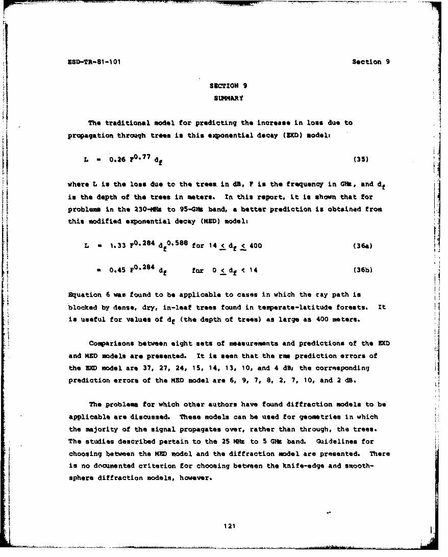
The traditional model for predicting the increase in loss due to
propagation through trees is this exponential decay (EXD) model.-
L - 0.26 F0 7 7 df
where L is the loss due to the trees in dB, F is the frequency in GHz, and df
is the depth of the trees in meters. In this report, it is shown that for
problems in the 230-44Hz to 95-GHz band, a better prediction is obtained from
this modified exponential decay (MED) model:
L - 1.33 F0"2 8 4 df 0 - 5 88 for 14 < df < 400
0.45 F 0 °2 8 4 df for 0 <_df < 14
The MED model is found to be applicable to cases in which the ray path is
blocked by dense, dry, in-leaf trees found in temperate-latitude forests.
Comparisons between eight sets of measurements and predictions of the EXU
and MED models are presented. It is seen that the rms prediction errors of
the EXD model are 37, 27, 24, 15, 14, 13, 10, and 4 dB; the corresponding
prediction errors of the MED model are 6, 9, 7, 8, 2, 7, 10, and 2 dB.
The problems for which other authors have found diffraction models to be
applicable are discussed. These models can be used for geometries in which
the majority of the signal propagates over, rather than through, the tries.
The studies described pertain to the 25-MHz to 5-GHz band. Guidelines for
choosing between the MED model and the diffraction models are presented.
There is no documented criterion for choosing between the knife-edge and
smooth-sphere diffraction models, however.
v
ESD-TR-81 -101
Kinase's empirical-theoretical model was found to be applicable to
problems where one antenna is located waell above the foliage. The model is
based on the assumption that the socond antenna is in an area n% of which is
covered with trees. n is an input parameter which can be varied from I to
50. Kinase's model is based on data in the 80 - 700 MHz frequency range.
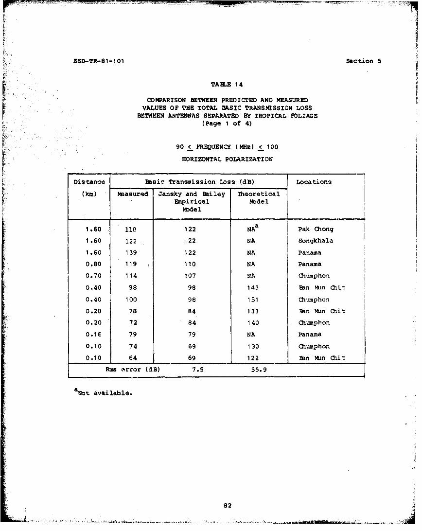
The Jansky and Bailey empirical model was found to be applicable to
problems where both antennas are immersed in a tropical forest. Path lengths
can vary from 8 to 1600 meters, frequencies from 25 to 400 MHz. Antenna
heights should he less than 7 meters. A comparison between a limited set of
measurements and predictions of the Jansky and Bailey empirical and a lateral-
wave theoretical model is presented. In this comparison, the empirical model
is seen to be more accurate. The theoretical model predictions were made
using measured values of the electrical parameters of the forests in which the
loss measurements were made. Use of effective values of these electrical
parameters appears to increase the accuracy of the theoretical model, but no
guidelines for determining such values have been reported.
A review of tropical and nontropical measurements showed that, very
often, the field strength at an antenna that is moved through foliaqe will be
Rayleigh distributed. Thus, circuit performance calculations should account
for this multipath-fading behavior in addition to accounting for the median
foliage loss. Euations for computing bit-error rates for signals subjected
to frequency-flat Rayleigh fading are presented for FSK and PSK.
vi
S-,. - -- ~.~---4'.----- -
ESD-TR-e1-101
GLOSSARY
symbol Word Definition
Basic transmission The ratio of the powerloss (ratio) in the input to a losslessabsence of foliage isotropic transmitting
antenna to the power
available at the terminalsof a remote lossless
isotropic receiving
antenna. I is a valuebo1that is computed or measured
with no trees between the
transmitter or receiver.
Basic transmission 10 log XboLbo
loss, dB, in the
absence of foliage
df Depth of foliage, meters The depth of the trees
between the transmitter and
receiver, in meters.
a Differential attenuation This quantity is determined
due to foliage, dB/meter by first subtracting the loss
on a path without trees from
the loss on a comparable path
with trees. The result, in
dB, is divided by the depth
; •of the trees, in meters.
vii
ES o..,R .e8 -10o1
symbol Word Def inition
Lb Basic transmission Lb + d
loss, dB, with foliage
EXD Model Exponential decay model A model based on the
assumption that a will not be
a function of the depth of
trees*
MED Model Modified exponential A model in which a is
26 True tree heicht minus effective obstacle height required to
obtain accurate diffraction loss calculation...... .......... 74
27 Kinase's estimate of the additional loss due to foliage and
man-made structures that cover n% of the surface area ....... 76
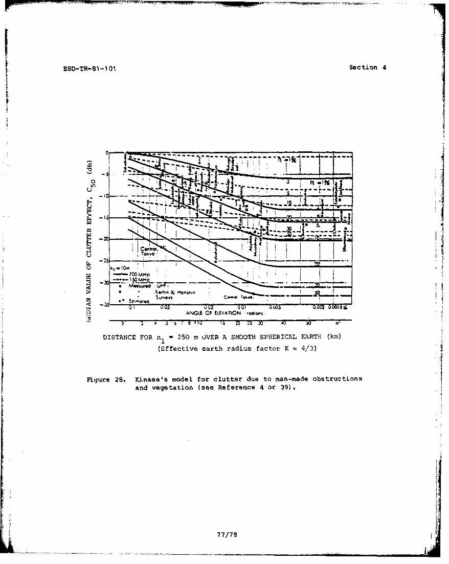
28 Kinase's model for clutter due to man-made obstructions
ýind ve e a i n. . . . . . . . . . . . . . . . . . . . . . . .77
29 Additional loss due to foliage vs frequency -- one
antenna blocked by a 60-90 meter grove ..................... 92
30 Additional loss due to foliage vs frequency -- extensive
grove of trees, no clearing. .. . ......... .................. 93
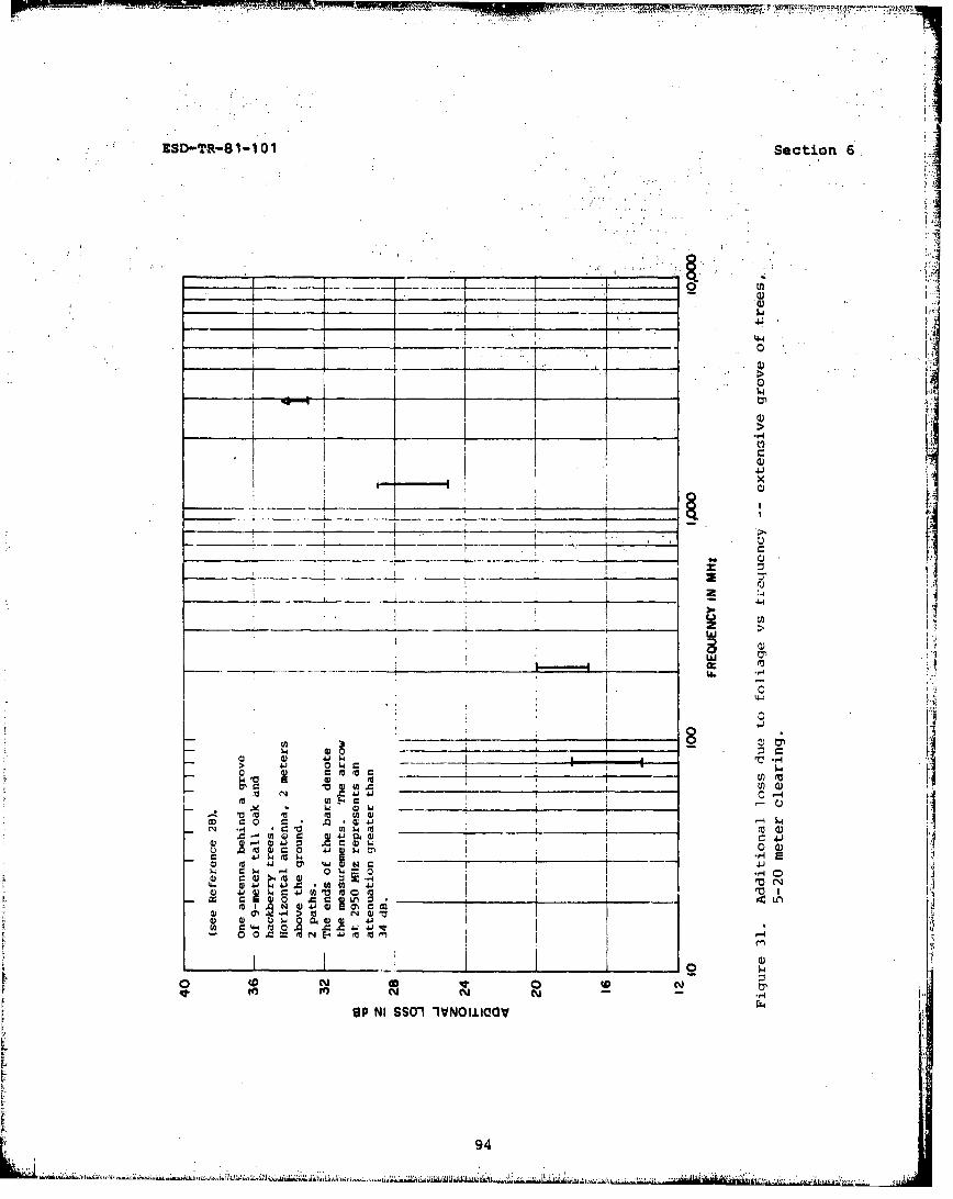
31 Additional loss due to foliage vs frequency -- extensive
grove of trees. 5-20 meter clearing ......................... 94
xiv
[- -
ESD-TR-81 -101
TABLE OF CONTENTS (Continued)
Figure Pg
LIST OF ILLUSTRATIONS (Continued)
32 Additional loss due to foliage vs frequency -- extensive
grove of trees, 35-65'meter 9a........................5
33 Additional loss due to foliage vs frequency -- one
antenna immediately behind a, single tree... ... . ...,........ 96
34 Additional loss due to foliage vs frequency -- both Iantennas immersed in a tropical jun9le, antenna separation.0.3 .. . . . . . . . . . . . . . . . . . . . . . . . . .97 i
35 Additional loss due to foliage vs frequency -- both Ij
antennas immersed in a tropical jungle, antenna separation
A ALTERNATE FORMULATIONS FOR a FOR THE EXD MODEL.. .............. 23
LIST OF REFERENCES 135 1
ii
XVi i/xviii iIJ
ESD-TR-81-101 Section 1
SECTION I
r INTR CDWTI 0N
101 BACKGR JND
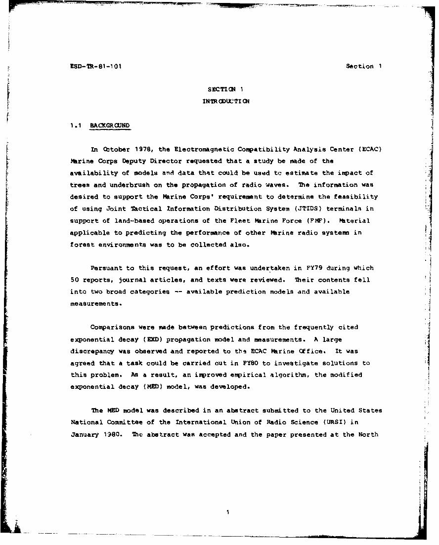
In October 1978, the Electromagnetic Compatibility Analysis Center (ECAC)
Marine Corps Deputy Director requested that a study be made of the
availability of models and data that could be used tc estimate the impact of
trees and underbrush on the propagation of radio waves. The information was
desired to support the Marine Corps' requirement to determine the feasibility
of using Joint Tactical Information Distribution System (JTIDS) terminals in L.I
support of land-based operations of the Fleet Marine Force (FM). Material
applicable to predicting the performance of other Marine radio systems in
forest environments was to be collected also.
Persuant to this request, an effort was undertaken in FY79 during which
50 reports, journal articles, and texts were reviewed. Their contents fell
into two broad categories -- available prediction models and available
measurements.
Comparisons were made between predictions from the frequently cited
exponential decay (EXD) propagation model and measurements. A large A
discrepancy was observed and reported to tbs ECAC Marine Office. It was
agreed that a task could be carried out in FY80 to investigate solutions to
this problem. As a result, an improved empirical algorithm, the modified
exponential decay (MED) model, was developed.
The MED model was deacribed in an abstract submitted to the United States
National Committee of the International Union of Radio Science (URSI) in
January 1980. The abstract was accepted and the paper presented at the North
4
11
A _..__._._ _ _ _
ZSD-TR- 81-1 01 Section I
American Radio Science ?4eting. A formal document was prepared for thelMarine Corps Developmenc and Education Command later in the year. 2
Subject to the l/.mitations documented in References 1 and 2, the MED
model was accepted by the Study Group 5 of the International Radio
Consultative Committie (CCIR). 3
In FY81, the material in the Consulting Report (see Reference 2) was
expanded and redocumented in the form of this Technical Report. The reasons
for this action were as follows.[!1. Readers of the Consulting Report had requested more evidence to
support the conclusions in that document.
2. The acceptance of the MED model by the CCIR had led to a need for
a report that described the basis and limitations of the model and that was
accessible to the international radio-engineering community.
II
Weissberger, M. and Hauber, J., "Modeling the Increase in Loss Caused byPropagation Through a Grove of Trees," Program and Abstracts of the NorthAmerican Radio Science Meeting, Quebec, Canada, 2-6 June 1980.
2Weisserger, M.A., An Initial Critical Summary of Models for Predicting theAttenuation of Radio Waves by Foliage, ECAC-CR-80-035, ElectromagneticCompatibity Analysis Center, Annapolis, MD, July 1980.
3 International Radio Consultative Committee (CCIR), Influenceof Terrain Irregularities and Vegetation on Tropospheric Propagation,Report 236-4 (MOD F), Doc. 5/5007-E, 7 September 1981.
2
ESD-TR-81-1 01 Section I
1 2 OBJECTIVE
The objective of this effort was to present an integrated description of
the FY79-FY81 ECAC study of the effects of trees aid underbrush on radio-wave
propagation.
1.3 APPR(.CH
7he information gathered during the study was organized into the
remaining eight sections of this report.
Section 2 is a review of the models and data that can he used to predict
the attenuation caused by propagation through (rather than ovt\r) groves of
trees that are as deep as 400 meters. It is shown that the expqnential decay I(EXD) model, though generally assumed applicable to such problea4, is often
inaccurate. The MED model is presented as a means to overcome so*m of the
problems with the EXD algorithm. Coaarisons between MED predicti.-ns, EXD
predictions, and measured data in the 230-MHz to 95-GHz frequency range are
documented. An approximate rule for determining which antenna-tree geometries
will be conducive to propagation through the trees (and MED applicability) is
developed.
Section 3 is a sumrmary of data relating to paths in which the trees are
far enough from both antennas so that the waves diffract over the forest. The
examples reported are in the 25-MHz to 5-GHz frequency range.
Section 4 contains a description of Kinase's model 4 for predicting the
loss that occurs when one antenna is elevated well above the forest and the
4Kinase, A., Influences of Tlerrain Irregularities and Evironmental ClutterSurrounding! on the Propagation of Broadcasting Waves in the UHF and VHFBands, NHK Technical Monograph No. 14, Japan Broadcasting Corporation,Tokyo, Japan, March 1969.
3
IM-TR-81 -101 Section 1
second antenna is located in a region, n% of which is covered with vegetation
or man-made structures. The basis for the model is data in the 80-700 4Hz
band.
Section 5 is a description of the Janaky and Baileys empirical model for
comuting the loss between two antennas immersed in a tropical jungle. Path
Lengths can vary from 0.08 to 1.6 km. The model applies to the 25-400 MJ~z
band.
Section 6 contains a collection of plots of measured foliage attenuation
versus frequency in the 2-MNz to 10-GRs range. Plots of attenuation versus
distance and attenuation versus antenna height are shown for the 900-12.00 MHz
band.
Section 7 is a summary of information relating to the variation of signal
strength with position that occurs when an antenna is moved through a
forest. It is seen that, very often, a Rayleigh distribution can be used to
categorize the variations.
Section 8 includes closed-form expressions for the bit-error rate that
can be expected for FSK and PSK transmissions when the signal strength is
Rayleigh distributed.
Section 9 is a summary of this report.
Differences between this report and the original Consulting Report
include the following.
5jansky and Bailey Engineering Department, Tropical ?ropagation Research,Final Report, Volume 1, Atlantic Research Corporation, Alexandria, VA,1966, AD660318.
4
ESD-TR-81-101 Section 1
! a. Additional data is presented to demonr,trate that the loss-
versus-frequency trend is more accurately predicted by the Mf) model than byS• other models.
b. Quantitative evidence has been included to demonstrate that the
Jansky and Bailey empirical model is a reasonably accurate means of predicting
the attenuation of VHF signals coupled between low antennas separated by
tropical foliage. Contrasts with another prediction procedure are alsopresented*
c. Summaries of three sets of measurement.s of the multipath-induced
spatial variability of signal strength in nontropical forests are presented.
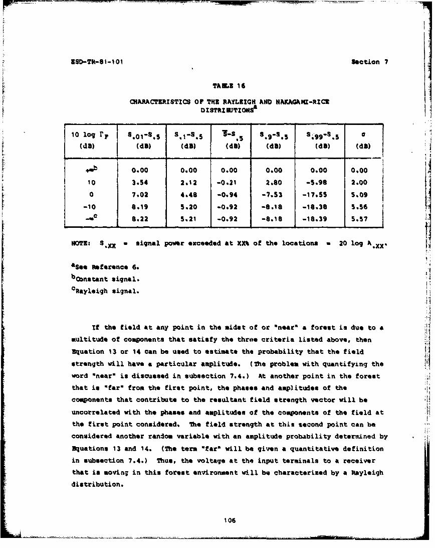
These complement the tropical data in the original documentation.do A clearer presentation of the percentiles of the Nakagami-Rice
distribution has been included. This is based on an earlier report by
Norton. 6
t
4Rice, P., Longley, A., Norton, K., and Barsis, A., Transmission LossPredictions for Tropospheric Comm.munications Circuits, NBS TN 101, NationalBureau of Standards, Boulder, CO, Revised January 1967.
5/6
m
8ED-T -•i-101 Section 2
SECTI ON 2
PRWIfCTING THE INCREASE IN LOSS CAUSED BY
PRc AGATION THROUGH A GROE OP TREESI
2e1 TUBE EMQNENTIAL DECAY (EXD) MODEL: BACKGROUND
1he traditional approach to modeling the additional loss caused by•, propagation through vegetation is to assume that this love increases
exponentially with the distance through the foliage. 7,8,9, 1 0, 1 1 Thus,
received power is calculated using:
P t gt gr "df
Pr J~bo
where
Pt transmitted power, in watts
Pr = received power, in watts
gt - transmitter antenna gain (ratio)
gr receiver antenna gain (ratio)
7Saxton, J*A. and Lane, J.A., *VHF and UHF Reception, Effects of Trees andOther Obstacles," Wireless World, May 1955.
8 LaGrone, Al.H, "Forecasting Televisicn Service Fields," Proceedings of theIRE, June 1960.
9Currie, NC., Martin, E.g., and Dyer, F.8%, Radar Foliage Penetration2tasurements at K llimeter Wavelengths, ESS/GI h-A-1485-TR-4, GeorgiaInstitute of Tchnology, Atlanta, GA, 31 December 1975, ADA023838.
1 0lnternational Radio Consultative Committee (CCIR), "Influence of TerrainIrregularities and Vegetation on Tropospheric Propagation," Report 236-4,XIV Plenary Assembly, International Telecommunication Union, Geneva,Switzerland, 1978.
1 1Krevsky, S., "HF and VHF Radio Wave Attenuation Through Jungle and Woods,"
IEEE Transactions on Antennas and Propagation, July 1963.
7
RSD-TR81 -101 section 2
ak< basic~l transmision1 loss i1n the absence of foXliage (ratio)hoal - differential attenuation due to foliage, in meter 1
df distance through the foliage, in meters.
Equation I describes the flow of electromagnetic radiation through an
infinite medium composed of either a lossy dielectric continuum or a
collection of randomly located discrete lousy scatterers. 2 A variation of
the equation was used by Bouguer in 1729 to describe the propagation of lightthrough liquids.
In logarithmic units, Equation 1 becomes:
(2)
where PR and PT are in dB, GT and GR in dBi, Lbo in dM, df in meters, and a
in dB/meter. a in Equation 2 is related to a, in Equation 1 by:
a - a, x 10 log e - 4.34 a, (3)
Values of a can be obtained from measurements using:
a- (1 - L2 )/df (4)
where
L, - the measured loss, in dB
L2 - the measured loss on a comparable path without trees, in dB.
Therefore, the additional dB of attenuation due to the trees on the path
is Qdf.
1 2 Ishimaru, A., Wave Propagation and Scatterins in Random Media, AcademicPress, New York, NY, 1978.
8 I
ESD-TR-81 -101 Section 2
Equations 1 and 2 describe a decay of the received signal (watts) due to
trees (or an increase in the loss due to trees) that varies exponentially with
df when a (and *a) do not vary with df. Models composed of Equation I (or 2)I
and a formula for a, (or a) that does not contain df will be called
exponential decay (EXD) models in this report. Subsection 2.2 contains
examples of this type of model. In subsection 2. 3, preliminary evidence is
"presented to show that for df ?. 15 meters,. a decreases with increasing df and, 4therefore, the EXU model is not valid here. An empirical "modified
exponential decay" (MED) model, that accounts for this behavior of a, is
described. In subsection 2.4. predictions from the N4ED and EXD models are
shown in comparison with measured values. It is seen that the NED model is Iconsistently more accurate.
2. 2 EXAMPLES OF EXPONENTIAL DECAY MO0DELS REPORTED IN THE LITERATURE]
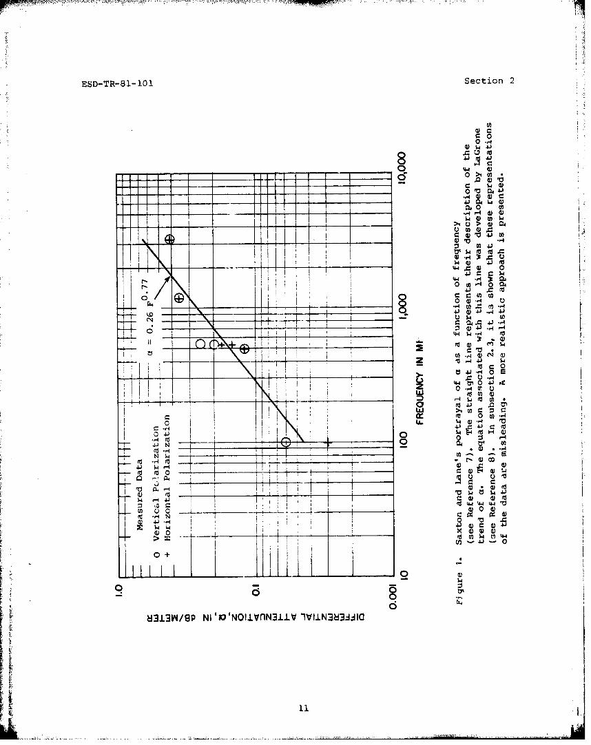
Saxton and Lane (see Reference 7) summarized groups of measurements taken
by Saxton, Trevor,'1 3 and IHoPetrie 1 4 in nontropical deciduous woods. In
TABLE 1, the subset of this data that relates to propagation through dry
(i.eo., not rained upon), in-leaf trees, is provided. Saxton used Equation 4
to compute values of a and plotted them in a manner similar to that shown in
Figure 1. LaGrone (see Reference 8) documented this analytical expression for
Saxton, a plot:
a 0. 26 F0.77 (5) I
"1 3Trevor, B., "Ultra-High-Frequency Propagation Through Woods and Underbrush,"RCA Review, July 1940.
14%cPstrie, J.S. and Ford, L.H., "Some Experiments on the Propagation of9. 2-cm Wavelength, Especially on the Effects of Obstacles," Journal ofthe IEN, Part 1lia, London, England, 1946, p. 531.
•.•_ " 9
ESD-TR01l-1O1 Section 2
A
cc
S a
£04
U 9-
ad4 0C~0 '
00
va¶ ,JI~ ~ . 4_ _ _ _ _ _ _
3.4 *o
'~ E~0
o 0 n 00
cc 0 vq
00 0n 00 00
10
ESD-TR- 81-101 Section 2
))
44 u
4J C4J_44
____ ~ 0) 4JE
d4J-4~ 0) 0
z 0 -, tr~ U
.0 4J
4J W~ .-4"-
(a 0 0)I
___ d__ _ _) 4)
u 0 0an
oV 4 0 r H
*04) .*.-0
(1)0 t0) *W
___ _ ___ _ __54C5 W
833)13 NI __ ____ ____.
___ L 0 .... 0--
ESD-TR-81-101 Section 2
where
a - the differential attenuation, in dB/m
F - the frequency, in GHz.
Alternative values for a were published in ensuing years -- one by
Krevsky in 1963 (see Reference 11), one in NE3 TN 101 (see Reference 6),15another in a paper by Rice in 1971, and a fourth in the CCIR Plenary-
approved reports (see Reference 10). Each is a form of the EXD model -- that
is, a is presented as being independent of the depth of trees, df. To allow a
compact presentation, quantitative examples of EXD predictions presented in
the main body of this report will be based on LaGrone's equation. Studies of
the alternate formulations are included in APPENDIX A.
2.3 THE BASIS OF THE MED MODEL
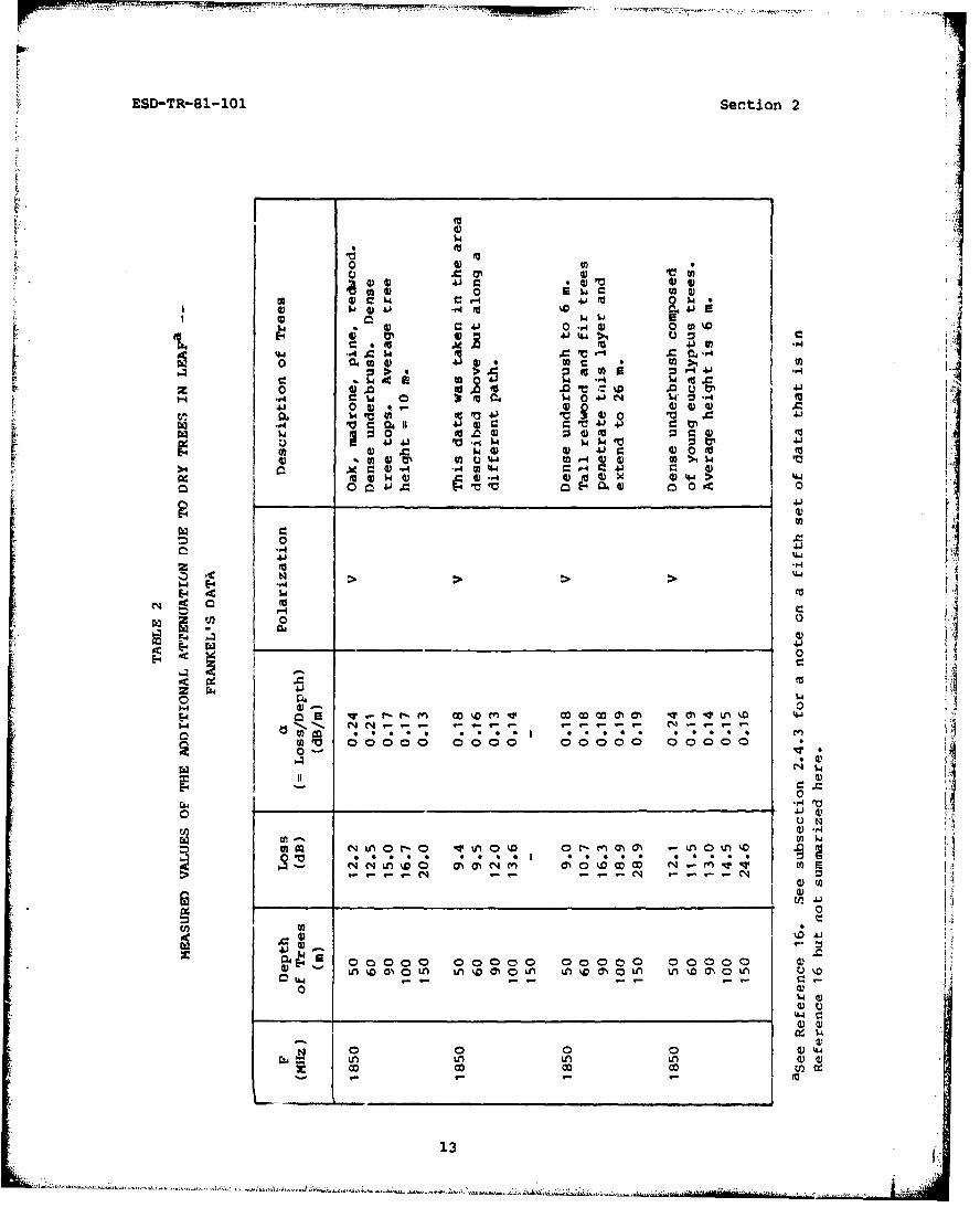
The EXD model is based on the data in TABLE 1, which extends in frequency ;_2
from 0.1 to 3.2 GHz and encompasses values of foliage depth (df) from 24 to
200 meters. As part of the ECAC study, predictions from the EXD model were
compared with measurements (different from those within TABLE 1) that fell
both within and beyond this range of frequency and df. One of the sets of
measurements that fell within the parameter range was collected by Frankel' 6
at several sites in west-central California. The data is listed in TABLE 2.
Figure 2 is a comparison between EXD predictions (a from Equation 5 times df)
and the measurements. It is seen that the agreement is poor with errors
ranging as high as 43 dB. Comparisons with other sets of measurements, which
will appear in later figures, showed similar problems.
1 5Rice, P.L., "Some Effects of Buildings and Vegetation on HF/UHFPropagation," Conf. Proc. of the 1971 IEEE Mountain-West Conference onElectromagnetic Compatibility, Tucson, AZ, November 1971.
s0 -- o-- Range of measured values.The measurements were collected Iby Frankel (see Reference 16), I I
S- IO , I II ,i
!50K1
I I
40 I , .l"•
0 0
S20 rj x
10 T T
010 100 2L0 300 1,000F, df (GHz. METERS)
Figure 2. Graph illustrating the errors that may arise when the E modelis used. The MED model, as will be shown, mitigates theseproblems. The frequency is 1850 MHz and the polarization isvertical. The x-axis of this graph is the product of frequency(F) in GHz and the depth of trees (df) in meters. Ihisparameter was selected because the applicability of the EXD
model can be more readily described in terms of ranges of F. dfthan it can be by individual ranges of F and df.
141
ESD-TR-81-1 01 iectior 2
As early as 19r8, Josephson1 7 had observed that the EMD nodel was not
applicable for prediction of loss through large depths of trees in temperate
forests. However, he provided no substitute computational procedure. Reviews
of the literature by this author and others1 0 ',1 8 revealed that no one else had
reported a successful alternativeea Therefore, the MED model was developed to
mitigate the problems associated with the use of the EXD model. T0%. MEZJ model
was first documented in an abstract submitted in January 1980 for a paper
presented later in that year (see Reference 1). The development of this model
will now be described.
Figure 2 demonstrates that use of the EXD model could result in
substantial errors. Figure 3 shows one source of the problem -- namely thatthe measured differential attenuation, a, decreases as the .iepth of trees |
increases. The EXD model is bised on the assumption that a is not a function
of the depth of trees. 2hus, if the attenuation rate measured at 50 meters,
a - 0.21 dB/m, were used in the EXD model to predict the loss at 150 meters,
the predicted value would be 32 dB. IT contrast, the average measured loss at
150 meters is only 24 dB, corresponding to a - 0.16 dB/lm.
A key step in developing the MED model was quantify-ng the decrease of
a. The California data was not used to develop the actual MED equation,
because it was limited to a single frequency. The Saxton and Lane data was
unsuitable, because the measurements for each frequency were taken through a
depth of trees different than the depth for any of the other frequencies.
IaaEmpirical and theoretical procedures were developed for the 1-400 Mfz band
for the problem of antennas separated by a tropical j!ng_. Theseprocedures are discussed in Section 5 of tfis report.
17Josephson, B. and Blonquist, A., "'he Influenc,, of Moisture in the Ground,
Temperature and Terrain on Ground Wave Propagation in the VHF-Band," IRETransactions on Antennas and Propagatior, April 1958.
1 8 Nelson, R.A., UHF Propagation in Vegetative MWia, Final Report forProject 8998, SRI International, Menlo Park, CA, April 1980.
15
ESD-TR-81-101 Section 2
0 41 ~ - _____ _ _ _ _
-1 u a)Aj41
AF -.0 a-
>e -4 I
ow C4
WwwW'~ ___ __ :1(DH
d d,
ItI
!01 -M-
ESD-TR-81-101 Section 2
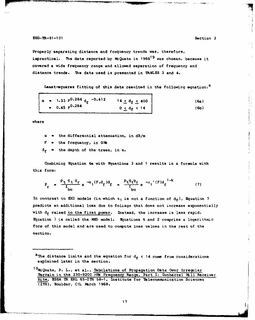
Properly separating distance and frequency trends was, therefore,
impractical. The data reported by McQuate in 1968i9 was chosen, because it
covered a wide frequency range and allowed separation of frequency and
distance trends. 7he data used is presented in TABLES 3 and 4.
Least-squares fitting of this data resulted in the following equation:a
a= 1.33 F0284 -0.412 14 < df _400 (6a)
a 0.45 F 0.284 0 <_dr < 14 (6b)
where
a - the differential attenuation, in dB/m
F - the frequency, in GHI
df - the depth of the trees, in m.
Combining Equation 6a with Equations 3 and 1 results in a formula with
this form:
p Pt gt gr -a (F,d f)df =Ptgtgr -1(F)d f 1-k (7)
bo bo
In contrast to EXD models (in which al is not a function of df), Equation 7
predicts an additional loss due to foliage that dons not increase exponentially
with df raised to the first power. Instead, the increase is less rapid.
Equation 7 is called the MED model. Equations 6 and 2 comprise a logarithmic
form of this model and are used to compute loss values in the rest of the
section.
aTe distance limits and the equation for df < 14 come from considerations
explained later in the section.1 9 McQuate, P. L., et al., Tabulations of Propagation Data Ove-r Irregular
Terrain in the 230-9200 MHz Frequency Range, Part I; Gunbarrel fill ReceiverSite, ESSA TR ERL 65-ITS 58-1, Institute for Telecommnnication Sciences(ITS), Boulder, CO, March 1968.
17
ESD-TR-81-101 Section 2
P0 f-.)
I- - a
be 4j4
Aa. .14 C
*j 0' 61 0
PU 89 4.441 u.g
E-6 E-4) 4) t8 2 C* m m0 mLn
Ln vLnen N m % - N N rC; C 8 C;C;
0 a61b LM LA %A r- 0
M 0 %n 0 04)4 06oo 16o14) n
en M * 0 m n v N 8
VU-M M% -M000 - N Vt n - r
0~~~ M__ ___________
6-18
ESD-TR-81-101 Section 2
r U4 IA 0
0 0% 4)404 '"
'.4 Q Al w 0 1.
41 4a 4 A 0 .4 4 "4 A 4)U4l44 U . 4 0 24
00
4P4
'.04
00.4)
cci
OMOOMO 00%O;NIO M 00 O
00-00000 0 000000% 0000000O
M L v .%L
N V- nMU
0M 0~0 ifaA 0N ~a~19u~
--7 -tw
ESD-TR-Cl1-101 Section 2
I.4U r-4
to u 0 FA
oili -0 0i*Iz 0 *
ba 14~b4 041 4 144 41*,III F4~
Lb o
4.)
AjC
F liii *.4
P
1 9
am-
U4)
N r-0 %ý 00 i r0u~ r, M r l- U)
ESD-TR-81- 101 Section 2
P4J
oo a, N R4A C
14 A0 1O U 0 a
Cuu C~4R u $4J IfI~
r0.
"E-4 04knNo % %. mr
C.FA0 aak W O Z 0r n0C
04A4eq1 N4N
MCnemo* ~ ~ L C4 v t- ON -.
*~~ ~~~~~ 00 0 0M00 0 0 0 0
U2
ESD-TR-81 -101 Section 2
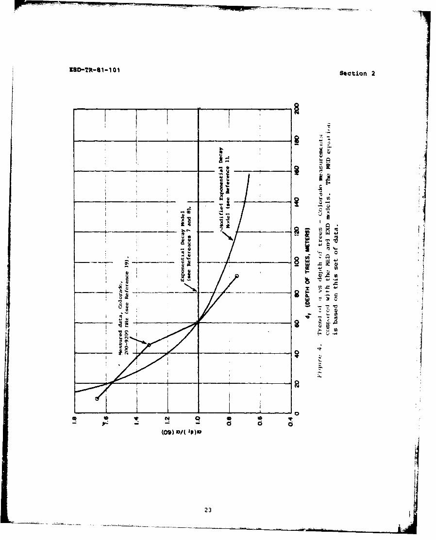
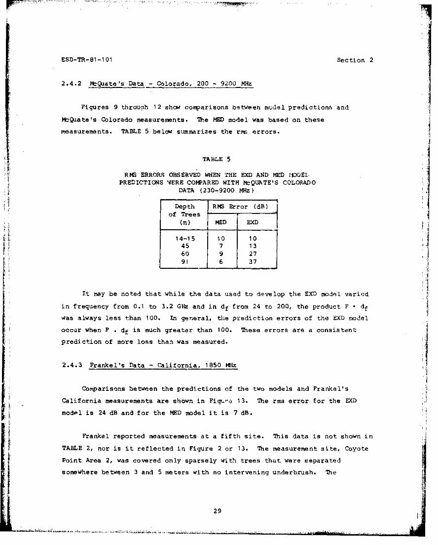
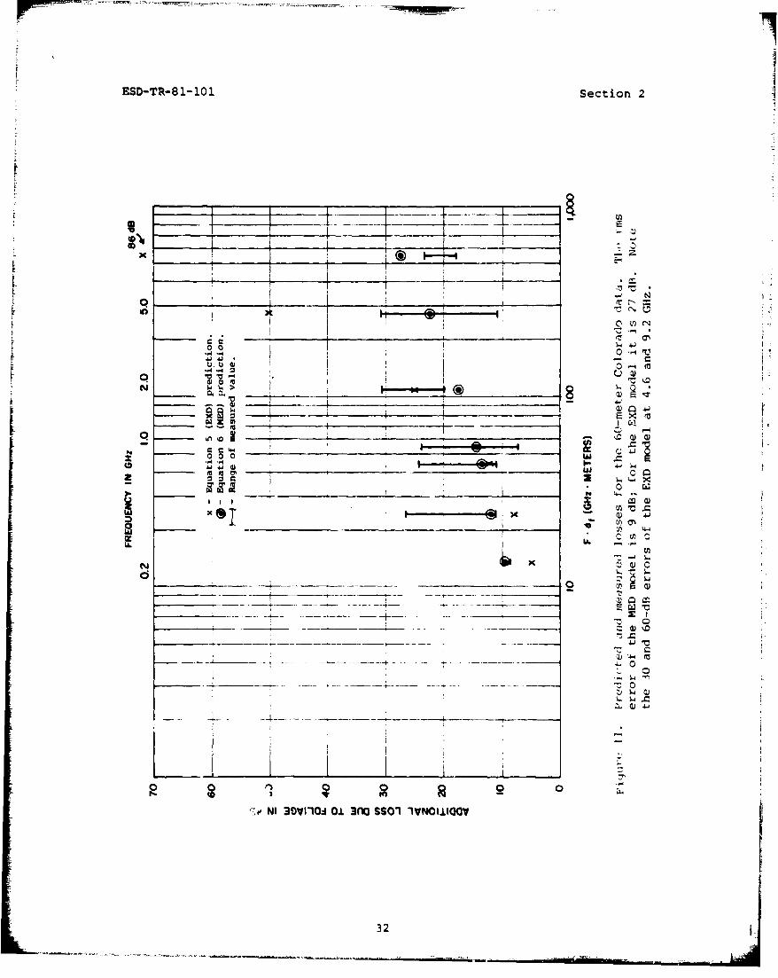
Figures 4 through 7 illustrate how the trend of a versus distance
predicted by Squation 6 cempares with four sets of measurements. Figure 4
shows the trend of the means of the Oolorado data. Good agreement is expected
here because the model is based fully on this data. The EXD trend is shown
for contrast. Figure 5 shows the comparison with the California data. The
agreement is reasonably good, even though this data was not used in the
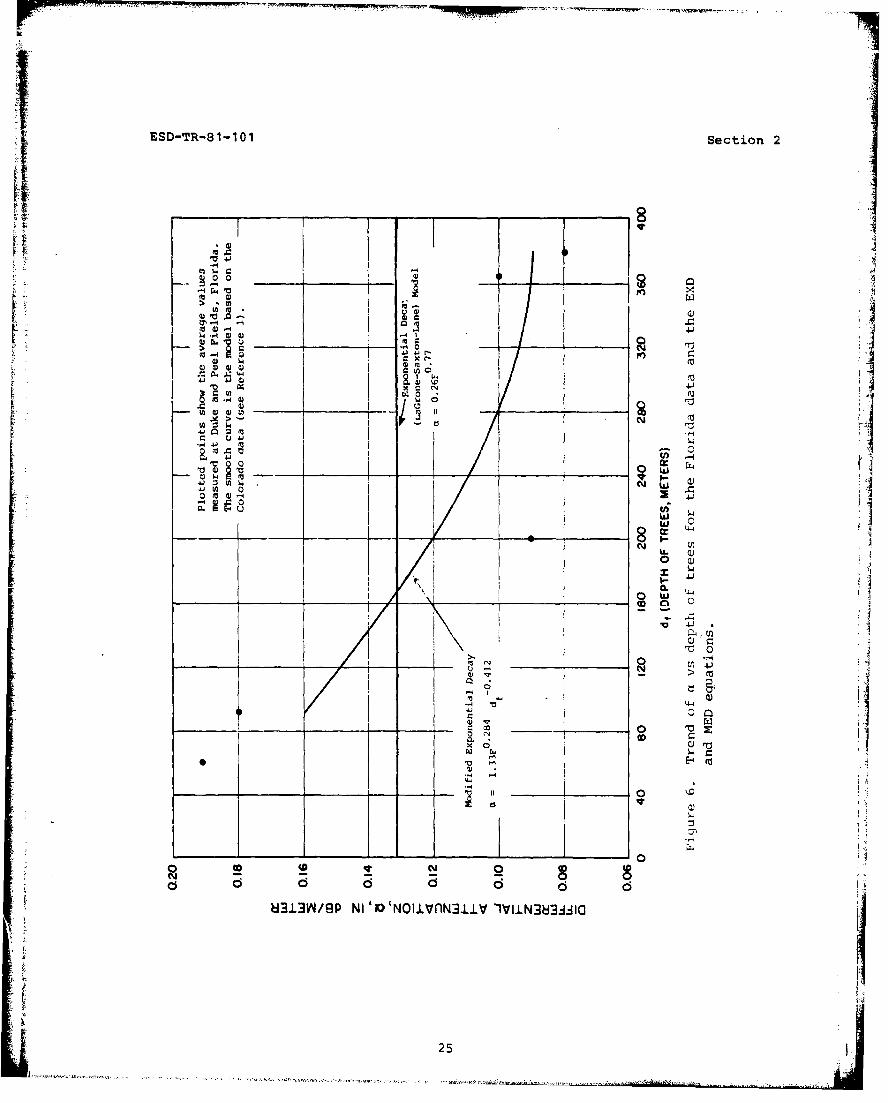
development of the model. Figure 6 shows the comparison with measurements
taken by the highes Aircraft Company in Florida at 400 oft.0 Again, the MED
model predicts the general decrease of a with distance, as was measured. The
EXD model does not.
IFigure 7 shows the trend of a versus depth of trees measured by
Currie 9 " 2 1 in Georgia at 9 and 16 GHk. It is seen that, at the short tree- I jdepths (0 < df < 14) reported, the measured values of a actually increase
slightly with increasing df. Possible reasons for this are discussed in
subsection ".5.2. Because of this observation and the lack of sufficient
information t - allow development of a general model for loss-versus-distance
behavior at these short distances, the decreasing a-versus-distance trend of
the MED model was modified for df < 14 to predict a constant a-versus-dLstance
trend (like the EXD model). This is reflected in Sjuation 6b.
2.4 VALIDATION OF THE MED MODEL
ht end of the previous subsection it was demonstrated that the MED model
predicted the trend of differential attenuation, a, versus distance more
2 0Kivett, J.A. and Diederichs, P.J., PLRS Ground-to-Ground Propagation TestTechnical Report (Draft), FR 80-14-6, 1bghes Aircraft Company, Fullerton,CA, January 1980.
0.3 - 6.7, and 0.3 - 6.7 meters. For this data, the rms prediction error of
the EXD model is 15 dB. For the MED model it is 8 dB.
Comparisons with measurements at tree depths larger than 400 meters
showed that the NED model consistently overpredicted loss. Since the equation
was based on data taken for tree depths less than 100 meters, inaccurate Vbehavior at much longer distances is not unexpected. The EXD model was less
accurate than the MED model at the large distances.
Comparisons were made with measurements taken at a third Florida site,Basin Bayou, where the tree density was much less than at the other two sites-- 5.1 m2 of trunk area per acrea versus 7.4 and 10. 2. Both the EXD and NEU
equations overpredicted the loss at this site.
aSome physical insight into the meaning of these values may be gained by
noting that in another Hughes report, the Basin Bayou area is described asone in which the vegetation was sparse enough so that you could walk throughit easily and ride through it, with care, on a two-wheeled vehicle. In thearea with the 10.2-mn2 trunk area density, walking would be difficult andriding not possible.
35
ESD-TR-8 1- 101 Section 2
to U
0
4j "4 -
F 0.. V~J'4 *#4' -H W
0 C 0 ~ 0,
so 6
~"4 W49
04 -HC4CC'bIN
CaM' a U -l
-- 7Ca 0
haa
'0 1
14 4
rCA .. r. A-
00 4 f" W14 ') r4 r4.
'~w-f44 fig *
H M
360
9SD..TR- 1 -10 1 Section 2
Restrictions on the use of the NED model that have been derived from
these and other observations are summarised in subsection 2.6.
2.4.5 The Georgia Institute of Technology Data - Georgia, 9,.4-95.0 G~z 1
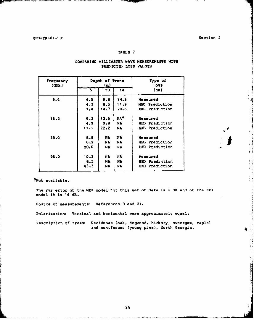
Currie (soe References 9 and 21) reported sea3urements of the attenuation
caused by propagation through deciduous (oak, dogwood, hickory, sweetgum,
maple) in-leaf trees, and coniferous (young pine) trees in northern Georgia.
TABLE 7summrizes his results. Currie's data was I::enawith a radar and
refectr.Hisvalesof the mesrdloss have been revised here to account
fo h sumto htthe attenuation for a normal communications link would
be oe-hlf f te vluemeaure wih aradar. Purthermore, the depth-of-
treevales avebee reise undr te asumtio tht astraight line
between the two antennas would intercept branches along 50% of its length. In
his reports, Currie endorses these approximations.
The predictions of the two modela are shown in TAMEB 7. The rms error of
the E)OD model is 14 d3 while the error of the NED model is 2 dB. It may be
noted that Saxton and Lane never recommended use of their empirical model at
frequencies greater than 3.2 Gft . However, it was used as a basis for
comparison in this 9.4 - 95.0 GH& study, because other authors (see References
9 and 21) have recommended it for use in this range.
2.4.6 Summery of Subsection 2.4
Cor~arisons of measurements and predictions from the MED and EXD models
have shown that the NED model is consistently more accurate than the EXD
model. Rme errors of the NED model were (from highest to lowest) 10, 9, 8, 7,
7, 6, 2, and 2 dB. For the W~O model the rms errors were 10, 27, 15, 24, 13,
37, 14, and 4 dB. The measurements all involved blockage of at least one
antenna by dry (i.e., not rained upon), dense groves of trees that were either
in-leaf deciduous or evergreen. The depth of the groves ranged from 2 to 400
meters. The vegetation was the type found in mid-latitude wooded areas.
37
EC.-TR-,81-101 Section 2
TABLE 7
COMPARING MILLIMETER W&VF MEASUREMENTS WITHPRW ICTM LOSS VALUES
16.2 6.3 13.5 NAa Measured4.9 9.9 NA MNE Prediction
11.1 22.2 NA EXD Prediction
35.0 8.8 NA NA Measured £6.2 NA NA NED Prediction
20.0 NA NA EXM Prediction
95.0 10.3 NA NA Measured8.2 NA NA NED Prediction
43.3 NA NA EXD Prediction
aNot available.
The rms error of the MED model for this set of data is 2 dB and of the EXMmodel it is 14 dB.
Source of measurements: References 9 and 21.
Polarization: Vertical and horizontal were approximately equal.
')escription of trees; Deciduous (oak, dogwood, hickory, sweetgum, maple)and coniferous (young pine), North Georgia. ,
38
LLi ,
ESD-TR-81-1 01 Section 2
There were three paths for which the MED model, while more accurate than
the EXD model, could not; be described as being applicable. Che involved tree
depths greater than 400 meters, and the other two involved sparse
vegetation. Further, no attempt was made to compare the model with
measurements taken at frequencies lower than 200 MHz.
2.5 FURTHER DISCUSSIa4 CF THE MED MCDEL
It has been demonstrated that the MED model is a worthwhile problem-
solving tool. Further discussion on the basis of the MED model follows. The
topics addressed are:
a. The mode of propagation that is described by the MED model
(subsection 2.5.1)
b. Tihe reasons for the loss-versus-distance dependence of the MED
model (subsection 2.5.2)
c. The justification of the frequency-dependence of the MED
predictions (subsection 2.5.3)
d. The justification of the lack of polarization dependence of the
MED model (subsection 2.5.4).
2.5.1 The Mode of Propagation Described by the MED Model
In subsection 2.4, it is demonstrated that the modified exponential decay
(MED) model provides a reasonably accurate description of five sets of
measurements. In this subsection, supplementary information concerning three
of these sets will be presented to demonstrate that the measurements represent
instances of propagation (at least initially) through the forest rather than
over the forest. This conclusion is used in subsection 2.6 to help define
antenna-forest geometries to which the MED model is applicable. a
In the Hughoms Aircraft Florida (see Reference 20) measurement program,
antennas were placed initially (see Figure 14) at opposite ends of a 400-ineter
grove of trees. Then both antennas were moved away from the trees until
39
ESD-TR-81-101 Section 2
H--40 . 400M - 40 -M
-I,
X X -- -- _ : :
4040'
X . X tX'1x I"".
00 0.20 Q40 20.40 40.40
RELATtVE CLLEARING LOCATION (G,C)
Figure 14. An experiment at 400 i4IZ (see Reference.20)demonstrating that a particular propagationpath starts through the strees rather than over them.If the path started over the trees, increasing theclearing size would have decreased the loss.This does not occur. Since the MED model doespredict the measured loss (* 4 dB), this constitutesevidence that the MED 'model applies to geometries inwhich the energy flow is, for the part of the ray pathnearest to an antenna, through the trees.
40 t;
ESD-TR- 81-101 Section 2
40-meter clearings existed at each end of the grove. The loss did not change
as the antennas were moved. Had the majority of the energy been propagating
over the trees, then the loss would have been reduced by at least 6 dB when
the antennas were moved away. This is because the angle over the tree tops
through which the rays would have had to diffract would have been
significantly reduced as the clearings were enlarged. Since no reduction in
loss was observed, this constitutes evidence that the energy propagatedprimarily through the trees. Signal transit-time measurements taken by Hughes
Aircraft confirm this conclusion.
In the California study, Frankel (see Reference 16' changed the mainbeam
orientation of the 15-dBi antennas used in the measurements. The greatest
received power was achieved when the horns were aimed at each other. Tilting
the antennas towards the top of the trees caused a decrease in the received
power. Again, this is -vidence that the majority of the energy propagated
through the vegetation.
The third set of measurements germane to this discussion is the one
reported by Saxton and Lane (see Reference 7). Saxton and Lane compared the
measured attenuations with the attenuations predicted by diffraction theory.
They concluded that the measurements were of propagation through the trees.
Because the MED modeL provided fairly accurate predictions (rms errors of
8, 7, and 2 dB) of these three sets of measurements, it is reasonable to
assume that the MED model describes propagation in which the antenna-forestgeometry is such that the power flow is, for the part of the ray path nearest
to tho an antenna, through the forest.
2.5.2 Notes on the Loss-Versus-Distance Trend
Figures 3 through 6 illustrate that for depths of trees (df) greater than
about 15 meters, the differential attenuation, a, in dB/meter, decreases as df
increases. A review of theory (see Reference 12) indicates that this type of
behavior does not generally describe propagation through an infinite medium --
whether it is filled with discrete scatterers or a lossy-dielectric
-. 41
ESD-TR-81-101 Section 2
continuum. Therefore, it is likely that the decreasing a is due to the finite
size of the region that offers the largest attenuaticn per meter.
It appears that this region of large attenuation per meter is the volume
filled densely with in-leaf (or in-needle) branches. Three cases can be cited
here to support this statement. One is Frankel's (see Reference 16) vertical
polarization data at 1850 MHz. He measured attenuation at a site where there
were only bare trunks between the -two. antennas.. Loss values for 60-90 meter
tree depths averaged 8 dB for this area in contrast to the 13-dB average for
the areas withi foliage. Figure, 15 illustrates the. second case. Here it is
seen that as the height o! a tree-obs trcted antenna is lowered from the
branchy region (- 8 meters) to the bare-trur~ka region below the branches, the
attenuation decreases by 20 ;dB.. In subsection '.7, data is summarizedindicating\ that the attenuation decreasas when leaves fall from the' Ibranches.. This data constitutes the t~ird case.
Therefor6', there .are regions cif lower loss on top ol (i.e., free space) -
and beneath (i.e., the bare trunk region) the high loss region. !t is
possible that while the ray. path starts in the lossy region of the trees
nearest to the antenna, a fYaction of the pat*, is in the lower Yoss regions. As:
If increases, the fraction grows larger and, therefore, the average value of aC
for.the path decreases.. The MED: moaet is an empirical description of this
decrease.
Kivett's (see Reference 20) 4C1'-,MHz measurements involved transit time as
well as attenuation. He noted that when the antennr, height: was lowered from
above to below the tree'tops, the transit time of the dominait sigualincreased. This suggests that, for his data, the low-loss route was across
the top of the trees.
A formal theoretical explanation of thý*s behavlor is not presently
available for frequencies greater than 200 MHz. (The lateral-wave model
provides one possible explanation for freque;icies belau 200 MHz and for very
dense tropical forests. See Section 5 of this report. )
42
ESD-TR-8 1 -101 Section 2
**U)
ISO
iT
1600 1 5 0 -S S .. ..u
E- tre - -u-k-Lo.sss through b
,,,, _ oss1hrouh branches"-m ;.with leavesi
IS
200 2 A 6 s 10 12 14 1* 10 20 22 24 26 2?
Antenna Height Above Ground, in m.
Figure 15. An example cE the loss cuused by propagation through bare trunksbeing lcwer than the loss through the branchy region: 9190 MHz,horizontal polarization. 2 2
"McQuate, P.L., Harman, J.M., and McClanahan, M.F., Tabulations ofPropagation Data Over Irregular Terrain in the 230-9200 MHz Frequency Range,Part IV: Receiver Site in Grove of Trees, OT/TRER 19, Institute forTelecommunication Sciences (ITS), Boulder, CO, October 197/1.i-1
43+• !W
ESD-TR-81- 01 Section 2
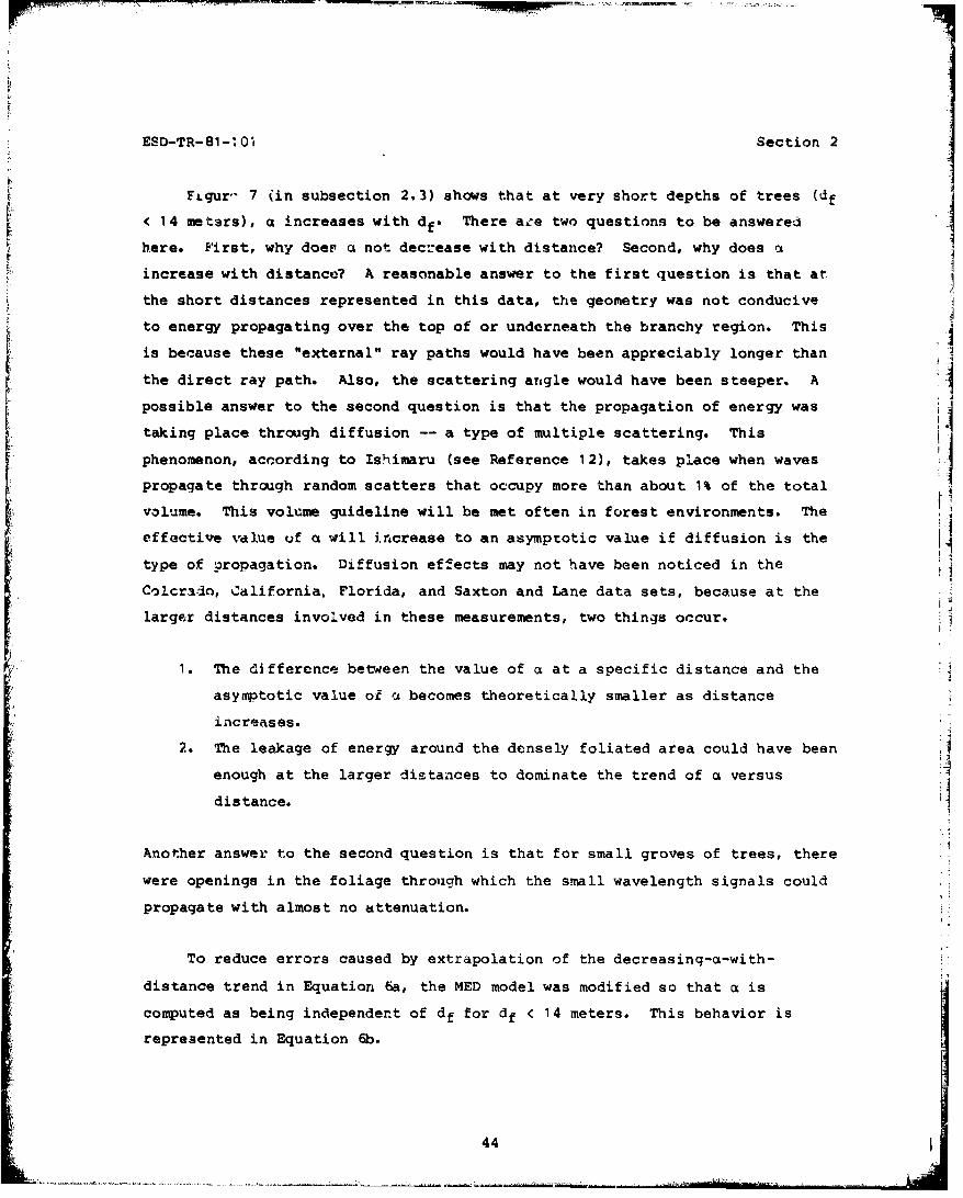
Figur- 7 (in subsection 2,3) shows that at very short depths of trees (df
< 14 metars), a increases with df. There aze two questions to be answered
here. First, why does a not decrease with distance? Second, why does a
increase with distance? A reasonable answer to the first question is that at
the short distances represented in this data, the geometry was not conducive
to energy propagating over the top of or underneath the branchy region. This
is because these "external" ray paths would have been appreciably longer than
the direct ray path. Also, the scattering angle would have been steeper. A
possible answer to the second question is that the propagation of energy was
taking place through diffusion -- a type of multiple scattering. This
phenomenon, according to Ishimaru (see Reference 1 2), takes place when waves
propagate through random scatters that occupy more than about 1% of the total
volume. This volume guideline will be met often in forest environments. The
effective value of a will increase to an asymptotic value if diffusion is the
type of propagation. Diffusion effects may not have been noticed in the
Colcra-o, California, Florida, and Saxton and Lane data sets, because at the
larger distances involved in these measurements, two things occur.
1. The difference between the value of a at a specific distance and the
asymptotic value of as becomes theoretically smaller as distance
increases.
2. The leakage of energy around the densely foliated area could have been
enough at the larger distances to dominate the trend of a versus
distance.
Another answer to the second question is that for small groves of trees, there
were openings in the foliage through which the small wavelength signals could
propagate with almost no attenuation.
To reduce errors caused by extrapolation of the decreasing-a-with-
distance trend in Equation 6a, the MED model was modified so that a is
computed as being independent of df for df < 14 meters. This behavior is
repreaented in Equation 6b.
44
ESD-TR-81 -101 Section 2
2.5.3 Justification of the Loss-Versus-Frequency Trend of the MED Model
The MED model was developed as an empirical means of accounting for the
observed dependence of differential attenuation on distance. Comparison of
MED Equation 6 with EXD Equation 5 shows that the former predicts that loss
will increase with frequency according to F0 2 8 4 , whereas the latter indicates
an increase proportional to F0 "770o Figure 16 illustrates the trends. The
magnitude of the difference between these relations can be better appreciated
by noting that the MED equation predicts that the lc'ss due to foliage at
4000 MHz will be 130% larger than the loss at 200 MHz. The EXD equation
predicts that the increase will be 900%. The questior. then arises as to why
there is such a difference and which is the more realistic model. Ahypothesis supporting the MED model is presented. Empirical verification for
the hypothesis follows.
It appears that the loss-versus-frequency trend predicted by the EXD
model is inaccurate because of the nature of the data on which it was based.
This data is the Saxton and Lane measurement set which appears in TABLE I of
this report. An examination shows that the higher frequency data was measured
through smaller tree depths, in general, than was lower frequency data. The
effective a's computed from this data were larger at the high frequencies for
two reasons. First, the loss due to a fixed amount of foliage becomes
greater, in general, as frequency increases. Second, at a fixed frequency,the dB/meter due to a small grove of trees is more than the dB/meter due to a
large grove. This is because, as has just been suggested, when the tree depth
increases, a higher percentage of energy propagates outside the highly
attenuating branchy region. Thus, since tree depth was not considered in the
development of EXD Equation 5, the empirically determined exponent of Fcarried the weight of two different phenomena. It appears that the developers
of Equation 5 would have arrived at a smaller (and more generally applicable)
value of the exponent of F if they had had access to measurements of signals
at many frequencies propagating through a single depth of trees.
45
ESD-TR-81 -101 Section 2
1.0 1 1IIz
Modified --- -____-
5 Exponential
Decay Mode
~( F070
(d u 50 meters)
Z.. 05
0t _______ A~Exponential Decay Model -
z_ _
W
U-u.
200 400 1,000 2P00 4,000
FREQUENCY IN MHz
Figure 16. The trends of a vs frequency for the Saxton-Lane-L&Grone EXD model and the MED model. Theexpression of the EXD model predicts that losswill increase 900% between 200 and 4000 Mz. TheMED model predicts a 130% rise over this range.Data studied indicate that the MED model ismore accurate.
46
ESD-TR-81 -101 Section 2
(Another contributing factor to the discrepancy between the two
relationships is the fact that they were developed, from data in different
frequency ranges. The EXD relations were developed from data at frequencies
as low as 100 M•. The NED relation is based on data at 230 M•z and above.
There is some evidence that F0 7 7 is an appropriate relationship at
frequencies of 100 MHz and below. 2 3 ' 2 4 )
Figures 17 through 20 represent empirical support for the hypothesis
that, at frequencies from 150 MHz to 95 GHk, the trend of loss versus
frequency is better described by F0 ' 2 8 4 than F0 "7 7 0 . A quantitative summary
of these figures is provided in TABLE 8. These rms errors were computed using
Equation 8. However, each error, E, is defined as a percentage using
Equation 10 below:
E.(%) Predicted loss (dB) - Measured loss (dB) X 100% (10)S~Measured loss (dB)
Use of percentages prevented the high-frequency (and high attenuation) part of
the data from playing an unduely large role in determining the overall error
statistics.
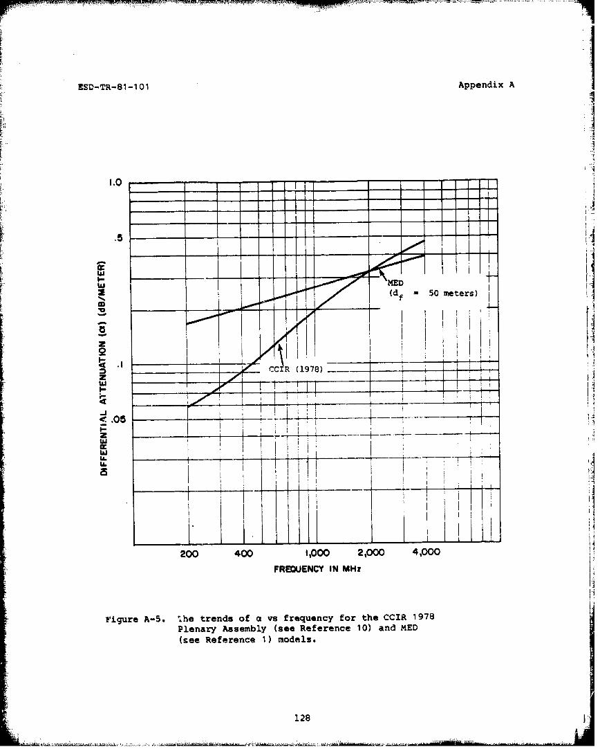
A comparison between the p0 . 2 S4 trend of the MED model and frequency
trends recommended by other authors (see References 6, 10, 11, and 15) is
provided in APPENDIX A.
2.5.4 Justification of the Lack of Polarization-Dependence of the MED Model
The measurements taken by KtQuate that form the basis of the MED model
were of horizontally polarized signals. It also appears that the model
provides a reasonable estimate of the attenuation of vertically polarized
signals in mid-latitude woods within the 200 MHz to 95 GHz band. This
subsection contains a summary of the observations supporting this statement.
2 3Hagn, G.H., SRI Special Tchnical Report 19, SRI, enlo Park, CA,January 1966, ,D484239.
2 4 Hagn, G.H., Research Engineering and Support for Tropical Communications.SRI, Menlo Park, CA, 1 September 1962, AD889169.
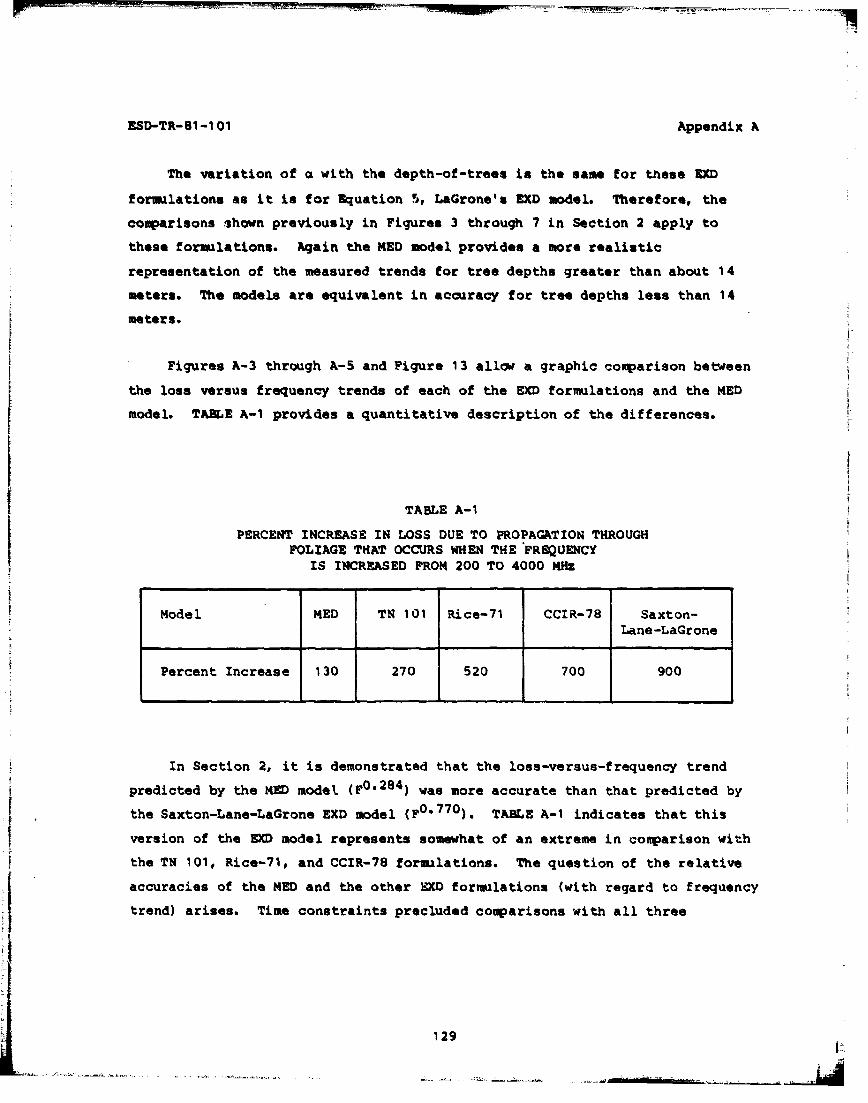
Figure 17. Illustration comparing the trends of loss vs frequency
predicted by two models with the measured values of thetrend. The rms error of the MED model is 26%. The error
of the Saxton-Lane-LaGrone model is 54%.
......................~ . -48
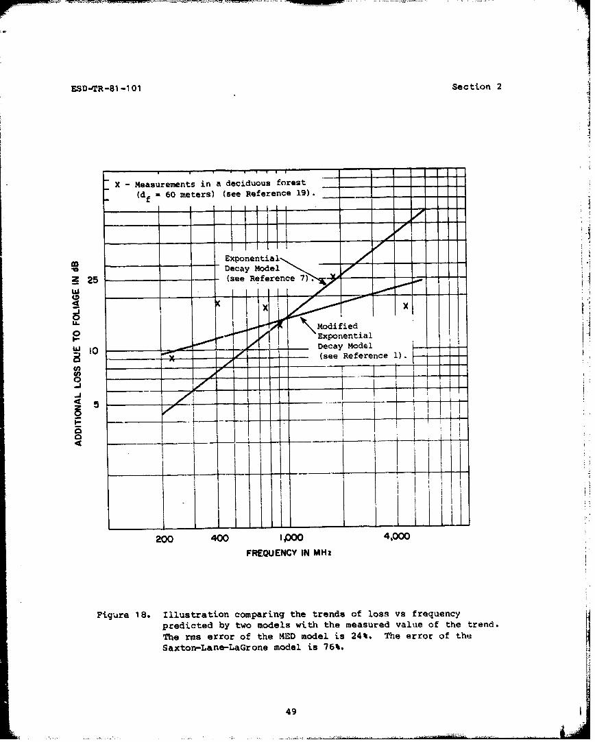
ESD-TR-81 -101 Section 2
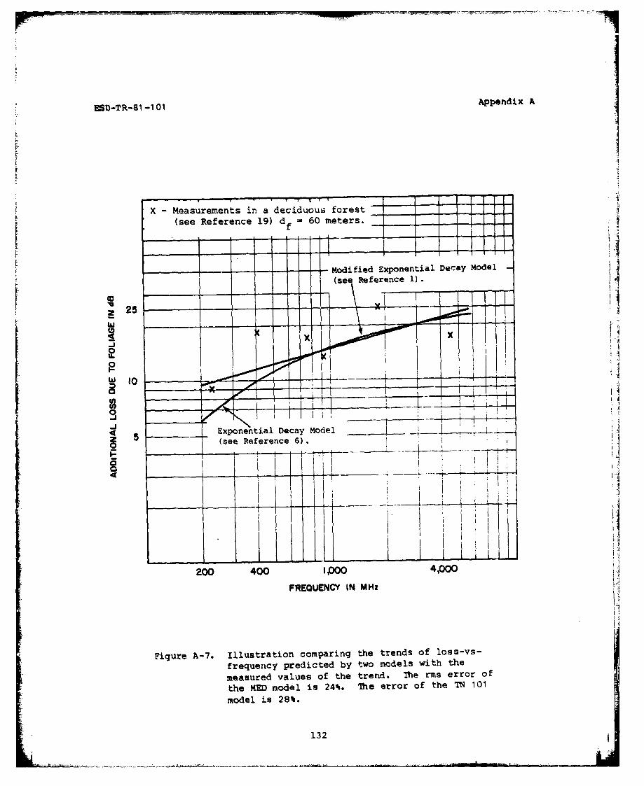
X - Measurements in a deciduous forest
(df - 60 meters) (see Reference 19). ._,
Exponential•
- - Decay Model
225 (see Reference 7). H_u
W I0 Decay Model(seReference1)
CD)0-j
I IL
200 400 I P 4,000
FREQUENCY IN MHz
Figure 18. Illustration comparing the trends of loss vs frequencypredicted by two models with the measured value of the trend.The rms error of the MED model is 24%. The error of theSaxton-Lane-LaGrone model is 76%.
49
ESD-TR-81 -101 Section 2
- .- Ti I
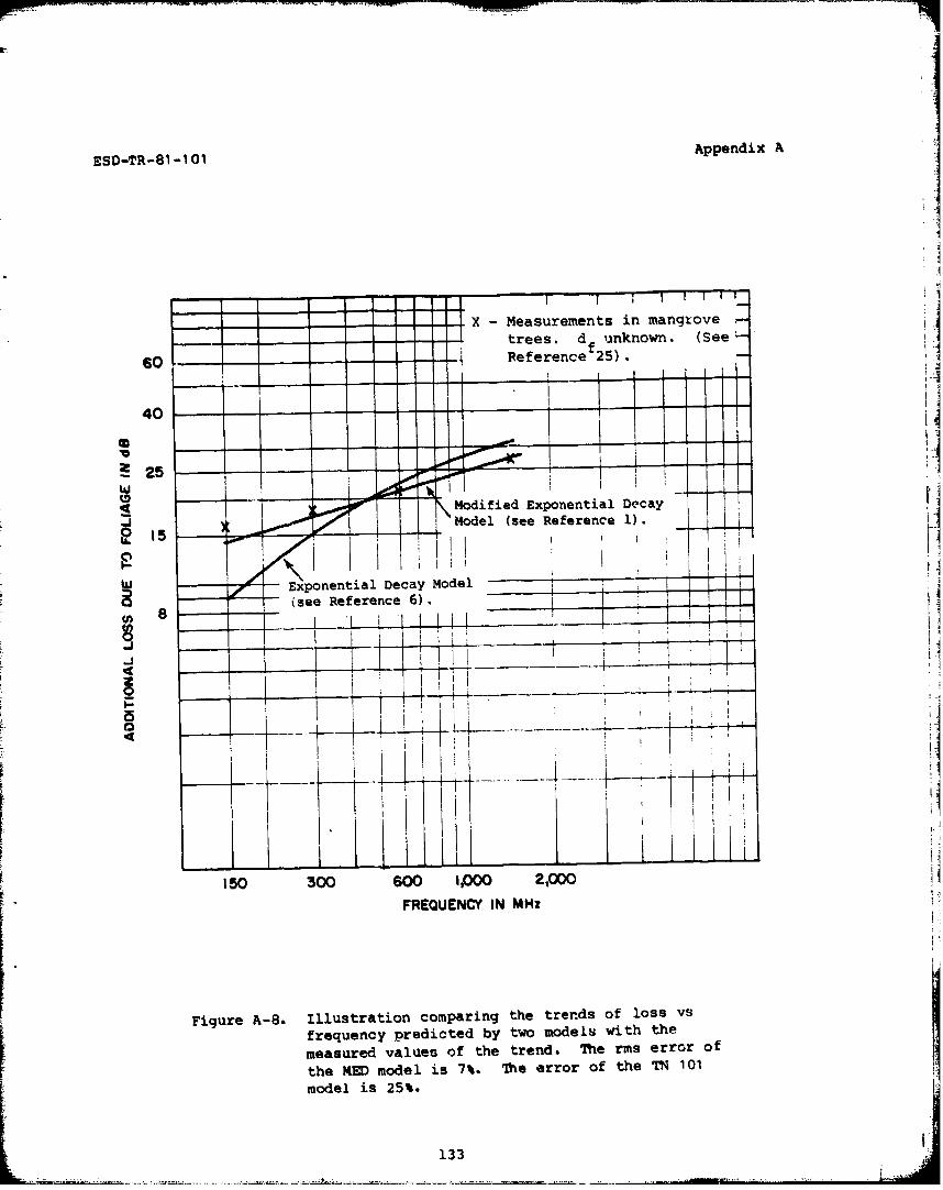
X - Measurements in
-0 mangrove trees60 (see Reference 25)
Exponential (df unknown).
Decay Model40 (see Reference 7).
25 - --
_ ~~~~Exponential --. t~~~oI• )Decay Model I1-5 (see Reference 1). i i
"r- 1 5 •:
F I
prdce bytomdlIihth esrdvleo
Figure -19. Illostraionsicompangtetroens of loss vsin fanroequnc
1/2 (loss ins f f mangroves)l i r
50
ESD-TR-81-101 Section 2
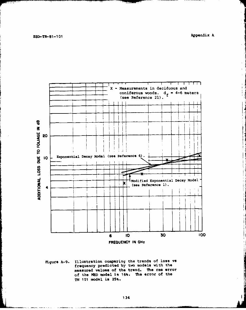
""-4 4 X - Measurements in Jdeciduous and -v
coniferous woods] ' i (df a 4-6 meters) -
..i (see Reference 21).
SI0 ! - *zz'z Decay Model.... .... •' r
_____ -- • (see Reference 1).'._... __ , !
20
J
•[1 Exponentionetaa ' 0
Decay Model
(seseern e 1eeene7.)
ji,'' iI I Iii,
6 t0 30 Ic'•)FREQUEN~CY IN GHu
Figure 20. Tllustrati'rn comparing the trends of loss vsfrequency predicted by two models with themeasured value of the trend. Th¶e rns error of
the ME•D model is 16%. ihe error of the Saxton-
Lane-LaGrone model is 39%.
i j
4 A.
ESD-TR-81-101 Section 2
TABLE 8
A COMPARISON OF THE RMS ERRORS OF THE NED ANDSAXTON-LANE-LaGRONE EXO MODELS WHEN THEY ARE USED TO
PRD• ICT LOSS -VERSUS-FREQUENCY TRENDS
A
Models UsedSaxton-Lane-
Data LaGroneDescription MED(E)
Deciduous forest, 26% 54%Colorado, 200-4500 MHz,horizontal polarization,df - 14-15 m
Deciduous and coniferous 16% 39%woods, Georgia, 9-95 GHzboth Polarizations,df 4-6 m
fiRms Error of
Predicted Trend
2 5Horwitz, C.M., "Optimization of Radio Tracking Frequencies," IEEETransactions on Antennas and Propagation, May 1979.
L52 52
ESD-TR-81-1 01 Section 2
These include:
1. Mihe model predicts the measurementa o'. vertically polarized
signals made by &ighes at 400 MHz (see TABLE 6) ani by SRI at 1850 M!z (see
Figure 13). ]2. The Georgia Institute of Technologo researchers observed no
difference between the attenuation of the two polar.Lzations in the
9.5-95 Git band (see References 9 and 21).3. Saxton ani Lane's data summary (see [ABLE 1) shows only a 2-dB
difference between the polarizations at 540 MHz. The 500 and 1200 MHz data
showed no differences. I4. Iiighes' measuremants 2 6 at 1 Glk showed that the average
difference between vertical and horizontal polarization was 1.5 dB.
As frequency decreases, the difference between the attenuation of the two
polarizations increases (see, for example, the 100-M~z data in TABLE 1). This
is one reason that it is not re'.commended that the MED model be used at
frequencies less than 200 MFz.
2.6 SUMMNRY OF N0£ES ON THE APPLICABILITY OF THE MED MODEL
2.6.1 Frequency and Depth-of-Trees Criteria
Figure 21 shows the frequency and depth-of-trees combinations fur which
Euation 6 (the MM model) has been shown to give reasonably accurate results
(rms error 10 dB or less). The model will predict too much loss if the depth
of trees is greater than 400 meters or if the frequency is below
200 MHz.
2 6 Hughes Aircraft Company, Final Report -JTIDS Ground Foliage Propagation1ý.sts, Technical Report FR-80-16-503, Fullerton, CA, April 1980.
53
ESD-TR-81-101 Section 2
1,000.,. -• .--.. ..
-. ".id boundaries (230 MHz, 400 meters) show
regions beyond which the model wiil nnt perform -
we.ll. Dashed boundaries indicate limits of avail- -_ able data. It is possible that the model will besatisfactory outside of these limits.
I..SI00
~Z Z Z / Z. Z Z. Z ,
w I0
,REQUZNCY IN G!
Fge1 OoAb
tempeate frestso54
O.,. .O100-FROCC I r
771,
1.0.
54
ESD- TR- 81 -101 Section 2
2.6.2 Clearing-Size Criteria
In subsection 2.5.1, it was demonstrated that the MED model applied to Iproblems in which the flow of power was primarily through the forest rather
than over the forest. Section 3 of this report will present diffraction
models 2 7 ' 2 8 ' 2 9 that apply to the problem .of propagation over the forest. This
subsection is a discussion of guidelines for determining which type of
algorithm is applicable.
The general guidance for predicting which algorithm should be used is
this: the M model will be applicable to problems in which one or both
antennas are very near to groves of trees that are less than 400 meters
deep. The diffraction model will be applicable to problems in which both
antennas are separated by a large clearing from a large grove of trees.
The most accurate approach to determinf- applicability is to compute the
loss using both methods. The more appropriate method is that which results in
the lower estimated loss for the particular problem.
A preliminary estimate of the result may be obtained by considering thetypes of problems for which the M model has been found to be accurate in the
past and the types of problems for which diffraction models have been shown to
be accurate. The clearing size is a parameter which can be used to describe
the different problems. The measure of clearing size that will be used in
this discussion is the take-off angle from the antenna that is nearest the
2 7 Head, H.R., "The Influence of Trees on Television Field Strengths atUltra-High 1requencies," Proceedings of tne IRE, June 1960.
2 8 LaGrone, A.H., "Propagation of VHF and UHF Electromagnetic Waves Over aGrove of Trees in Full Leaf," IEEE Transactions on Antennas and Propagation,November 1977.
2 9 Meeks, M.L., "A Low-Angle Propagation Experiment Combining Reflection andDiffraction," 1979 International Antennas and Propagation Symposium Digest,18-22 June 1979.
55
J1••"
CSD-TR-81-101 Section 2
trees to the tops of the trees. When one of the antennas is immersed in the
foliage, for example, this angle will be 900. As both antennas art- moved
farther away from the forest, this angle will approach 0*.
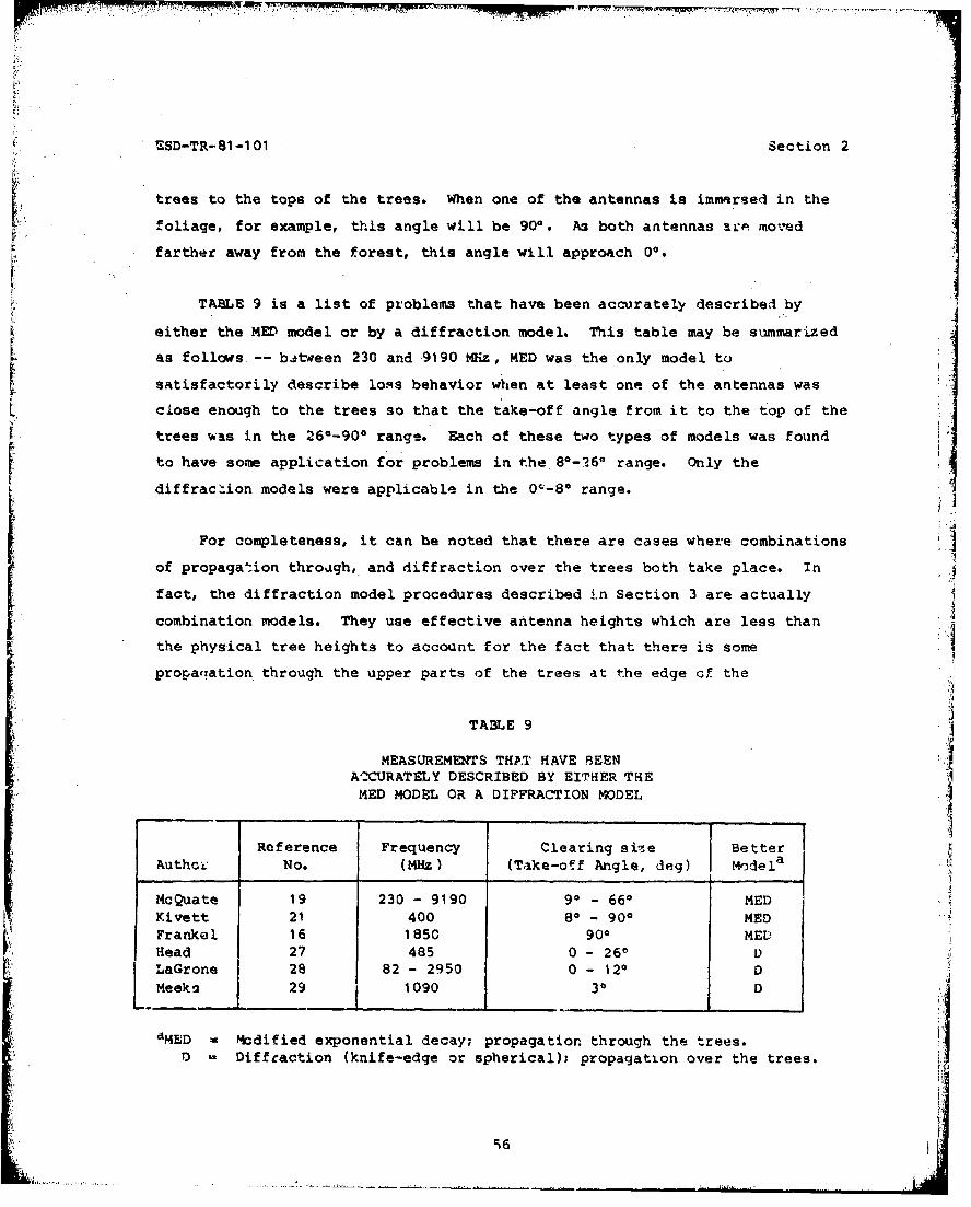
TABLE 9 is a list of problems that have been accurately described by
either the MED model or by a diffraction model. This table may be summarized
as follows.-- btveen 230 and 9190 MHz, MED was the only model to
satisfactorily describe loss behavior when at least one of the antennas was
close enough to the trees so that the take-off angle from it to the top of the
trees was in the 260-90* range. Each of these two types of models was found
to have some application for problems in the 8*-26* range. Only the
diffraction models were applicable in the 01-8* range.
For completeness, it can be noted that there are cases where combinations
of propagation through, and diffraction over the trees both take place. In
fact, the diffraction model procedures described in Section 3 are actually
combination models. They use effective antenna heights which are less than
the physical tree heights to account for the fact that there is some
propacTation through the upper parts of the trees at the edge cf the
TABLE 9
MEASUREMENTS THAT HAVE BEENA2CURATELY DESCRIBED BY EITHER THE
aMED - Modified exponential decay; propagation through the trees.-) Diffraction (knife-edge or spherical); propagation over the trees.
6I
ESD-TR-81-1 01 Section 2
30 230clearing. !ongley and the Hughes 2 6 researchers proposed their own
techlniques for combining "prcpagation over" and "propagation through"
models. Studies have not been conducted yet to determine which of the two
models is mote accurate.
2.6.3 Trunk-Density Criteria
The MED model applies to problems in which the ray path is blocked by a
dense grove of tzees. It was observed (subsection 2.4) that the model was
applicable to the FVorida data when the trunk density was 7.4 to 10.2 m2/acre
but not for cases in which the density was 5.1 m2 /acre. This was investigated
as the basis for developing a quar-titative defiaiition of "dense." Using data
reported by Ooeppker,31 calculations were done of the a .?oximate trunk
density in a wet-dry tropii:al forest. A value ot 3.3 m2/anre was obtained.
Since, as will be shown in subsection 2.7.' of this report, the attenuation in
this type ot tropical forest is much larger than in the tempelate forests
discussed previously, it does not appear that trunk-area density by itself is
a usef,.' indicator of the regions where N'ED Equation 6 will apply. The amount
of underbrush, actual nuniber of trunks per unit area, orientation of branches,
mcisture content of th-. "ood, iu.d Lypt of leaves are all fctcors oe potential
significance in determining the general applicability of an MED equation.
F1urther data related to the correlation between trunk density aA.Q loss is
provided by Presnell. 3 2 ' 3 3
30Loge,'Longlay, A.G. and Hufford, G.A., Sensor Path Loss Maasurements - Analysisand Comparison with Propagation Models, OTR-75-74, Institute forTelecommuniloation Sciences (ITS), Boulder, CO, October 1975.
3 1Doeppner, T.W., Hagn, G.H., and Sturgill, L.G., "Electromagnetic Propagationin a Tropical Environment," Journal of Defense Research, Winte.. 1972.
3Presnell, P.I., PLRS Ground-to-Ground Propagation Measurements, SRI Project8171, SRI, Menlo V'ark, CA, June 1900.
S-. ~~33,rselIresnell, PI., JTIDS Ground-to-Grour.d Propagation Measurements, SRI Project
6171, SRI, Mienlo Park, CA~, Jure 1990.
57
ESD-TR-81-10! Section 2
2.6.4 Antenna-Height Criteria
Since leakage over and under the brenchy region of the trees plays a role
in determining 13ss, factors such as antenna height, tree height, and
structure of the tross will also affect the loss. At present, there is not
enough data to allow development of a general model to account for thesefactors.
Further data relat.ed to the correlation between antenna height and lossi n a temperate forest is presented in the Hughes studies (see References 20
and 26).
2.6.5 Polarization Criteria!IIn light of the discussion in subsection 2.5.4, it is reasonable to
recommend the uae of the MED model for both horizontal and vertical
polarization predictions.
2.7 SUPPLEMFNTARY M4EASUREMENTS OF THE LOSS CACSED BY PROPAGATION THROUGH A
GROVE or TREES
In the preceding parts of Section 2, data haa been presented which
pertains to the attenuation caused by propagation through groves of dry, in-
leaf trees in temperkte mid-latitude for zsts. In this subsection,
measurements of the loss caused by propagation through groves of trees under
other circumstances are cited.
2.7.1 Tropical-Forest Data
Jansky and Baiiey researchers (see Reference 5) determined that
prcpagation through short (< 80 meters) distances in a Pak-Chong, Thailand,
jungle could he described by the EXD model, Equation 2. At these distances in
the 50-400 MHz band, it was found that Lbo was Lbfs, the free-space
58
ESD-TR-81- 101 Section 2
transmission loss. Measured values of a are listed in TABLE 10. The vertical
polarization data from TABLE 10 is platted in Figure 22; the horizontal data
is plotted in Figure 23. For comparison, Equation 6 is plotted as a dashed
line. It is seen that the jungle attenuation is 2 to 5 times larger than the itemperate-forest data represented by the equation.
(it is possible that an analysis of the raw Jansky and Bailey data would
show that a form of the MED model would be more accurate than the EXD model.
Such a study was beyond the scope of this effort. However, it can be noted
that the Jansky and Bailey researchers only recommended use of the EXDrelation for distances small enough so the F • df was less than 32. Figures 8
through 13 indicate that for this range, the MED model is not significantly
better than the EXD model -- at least in temperate forests.)
TABLE 10
EXPERIMENTAL VALUES OF a FOR h TROPICAL FOREST
F Depth a Polarization Description of Trees 34
(MHz) of Trees (- Loss/Depth)(i) (dB/m)
50 10 < df < 80 0.0 V - H Leafy jungle with heavy jundergrowth. Median
100 10 < df < 80 0.39 V tree diameter is 10 cm.0.17 H Mean separation between
trees is 1.3 m. Total250 10 < df < 80 0.43 V number of trees is
0.22 H 362 per acre. This isa semi-dry tropical
400 10 < df < 80 0.48 V forest. Annual average0.30 H temperature is 80.70 F.
Average annual rainfallis 63 inches.
3 4 Hicks, J.J., et al., Tropical Propagation Research, Final Report, Vol. II,Atlantic Research Corporation, Alexandria, VA, November 1969, p. 10.(See also Reference 31, p. 370, and Reference 5, p. 29.)
59
ESD-TR-81-101 Section 2
10.0
X Jansky and Bailey Data
(see Reference 5, p. 99). --------
S- 1.33 F0 2 8 4 df"0.412
(Temperate values computed
W for d , 45 meterc. ShownW•only for contrast.)"w 2
WiI I I
I I
Recommended values _ ,
for tropical jungles 1I.•,
0.1.0
1 0 100 1,000
FREQUENCY IN MHz
Figure 22. Differential attenuation due to oliage -tropical
jungle and vertical polarization.
60
ESD-TR-31-101 Section 2
10.0 -77_ _ A-
x Jaansky and Bailey Data
(see Reference 5, p. 99). -
0. 284 -0.412-- L f = . -F
(Temperate values computed
for df = 45 meters. Shown ---
only for contrast.)
o ,.o__,___
o I,
"a __ __ ,
1.0,
for tropical jungles. ;!
0.
7 7 - 1, i i L0ý
10 100 1,000
FREQUENCY IN MHz
Figure 23. Differential attenuation due to foliage --
tropical jungle and horizontal polarization.
61
ESD-TR-81-101 Section 2
The Jansky and Bailey researchers reported that losses at tree depths
greater than 80 meters were less than the EXD model predicted. Section 5 of
this report summarizes behavior at these larger distances In the tropical
forest.
LISection 5 of this report also includes a validation of the Jansky and
Bailey empirical model. Although no comparisons were made with data taken at
distances less than 80 meters, there were comparisons made with data in the
100-160 meter range. The values of a from TABLE 10 still play a significant
role in determining the predicted loss at these distances. A total of eight,
100-160 meter tropical-forest measurements taken at three sites (none of them
Pak Chong) were compared with the Jansky and Bailey empirical model
predictions. The mean error was -1.3 dBI the rms error was 8 d3. Thus, the
values of a shown in TABLE 10 appear to provide reasonable accuracy for
predicting attenuation at short distances in tropical forests at Pak Chong and
at other sites.
2.7.2 Leafless-Tree Data
Trevor (see Reference 8) found that the attenuation caused by 152 meters
of leafless deciduous trees with underbrush at 500 MHz was 15 dB for vertical
polarization and 12 dB for horizontal polarization. In contrast, the
attenuation for this same grove with leaves was 18 dB for both
polarizations. The corresponding effective . were 0.10 and U.08 dB/meter
without leaves and 0.12 dR/meter with leavs.
At 250 MHz, Trevor found that the attenuation through the same grove of
leafless trees was 14 dB for the vertical polarization and 10 dB for
horizontal polarization. No data at this frequency was taken for the trees in
leaf. However, for comparison, it may be noted that the MED equation
62
ESD-TR-81-101 Section 2
indicates a loss of 17 dB due to in-leaf trees at this value of frequency and
depth of trees. Sofaer and Bell 3 5 reported the data listed in TABLE 11.
TABLE 1)
LOSS DUE TO IN-LEAF TREES VERSUS LEAFLESS TREES
Description Freq. Pol. Additional Loss (dB)Of Trees (MHz) In Leaf Few Leaves
50 V ~0 -0
Large Grove 200 V 9 5
750 H 19 15
50 V -0 -0
Single Row 200 V 30 0
750 H 5.5 3
The Federal Communications Commission (FCC) reported3 6 that the
additional loss caused by leaves was 4.5 dB at 450 and 950 MHz. Values of the
depth of trees and of the comparable loss without any trees were not
reported. More data with these limitations appears in Reference 22.
I
35 Sofaer, E. and Bell, C.P., "Factors Affecting the Propagation and Receptionof Broadcasting Signals in the UHF Bands," Proceedings of the IEE, London,England, July 1966.
3 6 International Radio Consultative Commi.ttee (CCIR), Methods and Statistics
for Estimating Field-strength Values in the Land Mobile Services Using theFrequency Range 30 MHz to 1 GHz, Doc. USSG 5/D-11, 1981 (Submitted by theFCC)•
63
ESD-TR-81-101 Section 2
2.7*3 Data for Trees After a Rainstorm
The attenuation caused by propagation through a grove of trees that is
wet from rain is an important factor in determining system performance. Only
a small amount of data has been reported. This includes the following.
a. At 400 MHz, rain on 1000 meters of trees increased the
[ attenuation by 4 dB (see Reference 20).
b. At 1000 MHz, rain on 200 meters of trees increased the loss by
20 dB at low antenna heights. When the antennas were raised so that the
energy propagated across the top of the forest, the loss did not change when
it rained (see Reference 26).
c. The increase in loss in the 9.4-95 GHz band varied from 14 to 50L
dB. TABLE 12 is a summary of this data (see Reference 9).
TABLE 12
THE ATTENUATION DUE TO WET TREES IN LEAFa
F Loss Due to Foliage Polarization Description Depth of.(GHz) (dB) Trees (mn)
Wet Dry (Approximate)
9.4 19.0 4.5 V Z H Deciduous trees 5(oak, dogwood,
16e2 25.5 6.3 V 19H hickory, sweet- 5gum, maple);
35.0 30.9 8.8 V 1 H North Georgia. 5
95.0 60.6 10.3 V H 5
aSee Reference 9, Figures 21 and 22.
64
ESD-TR-81 -101 Sec tion 2
2.8 Su•MMAY OF SIrON 2
If a transwitted signal propagates through • grove of trees df meters
deep, the mean received power can be estimated with this equation:
i- T + %+ -L -df (2)
It has been shown, that for propagation through the branchy region of dry
temperate forests with trees in leaf, the attenuation coefficient, a, can be
computed by this NED equation:
1., 3 F f- 4 < f ý.400(6a)
0.45 F0"284 0 <_dr < 14 (6b)
Equation 6 was developed from measurements of the attenuation caused by
propagation through deciduous trees in Colorado. Comparisons with
measurements demonstrated that this equation is more accurate than the
commonly reported EXD equation:
a= 0.26 F 0 " 7 (5)
The data examined in the comparison was taken in England, Pennsylvania,
California, Georgia, Florida, and Colorado,
The MED equation was shown to be applicable in the 230 kHz to 95 GHz
frequency raage and for groves of trees as deep as 400 meters. Figure 21
shows the frequency-depth combinations that were examined.
aAs final typing of this report was being completed, a study prepared by
E. J. Violette of the Institute for Telecommunication Sciences was received.TABLE 4.3 of the document, CECOM-81-CS020-F, June 1981, contains measurementsof a at 9.6 - 57.6 GHz. The trends of these values au a function of F and dfare quite close to those predicted by MED Equation 6. However, the actualvalues are notably larger than the predictions. They are also larger thanCurrie's and McQuate's measured values in this frequency range. A study toresolve these differences is desirable.
65
SSD-TR-81 -10 01 Section 2
Th~e equation is applicable to dense, temperate, mid-latitude forests.
There is presently, however, no dependable means of quantifying density.
The equation is applicable when at least one of the antennas is within or
near the grove of trees. An approximate criterion for being n~ar the trees is
that the take-off angle from the antenna nearest the trees to the tree tops is
greater than 160. in somte instances, however, the model was found to be
applicable for angles as low as 80s It is desirable to compute the 14 loss
and the diffraction loss (described in Section 3) for each specific problem.
The appropriate model will be the one with the lower predicted loss.
if the foliage is wet from a rainstorm or if it is characteristic of
tropical areas (very lush and with heavy underbrush), then a will be larger Ithan is predicted by Equation 6. If the~re are no leaves on the trees, Q will
be smaller. Available data for these circumstances is presented in
subsection 2.7.
66
ESD-TR-81-101 Section 3
SECTION 3
DIFFRACTION OVER TREES
3.1 INTRODUCTION
This section summarizes reports of cases in which it was found that tilp
characteristics of loss were predicted by the assumption that the majority of
the energy propagated was caused by diffraction over the trees.
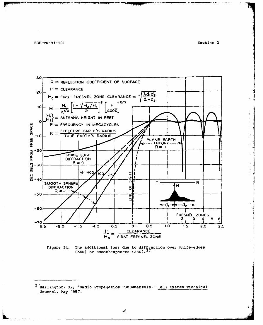
Figure 24 illustrates the basic parameters for a diffraction
calculation. While the fic'-e shows that the calculations can be done for a
continuum of geometries, reptrts on the model have only dealt with two
extremes: the infinitely narrow obstacle -- knife-edge diffraction (KED)
and the smooth-spherical obstacle with a radius equal to 4/3 times the true
radius of the earth.
With the l.imited amount of information available, it has not been
possible to develop a precise criterion for determining when the KED model
should be used and when the smooth-spherical diffraction (SSD) model is
applicahle.'I
3.2 HEkD -- THE SSD MODEL
HeaJ's study (see Reference 27) discusses two models. One, the SSD that
requires knowledge of the specific antenna-forest geometry, and the other, a
type of "area" model in which the details of the location of the trees in
relation to the antennas are not required. In this subsection, Head's
findings on the SSD model are summarized. His area model is discussed in
Section 4 of this report.
67
ESD-TR-81-1 01 Section 3
30- --
R REFLECTION COEFFICIENT OF SURFACE
H = CLEARANCE20-
Ho = FIRST FRESNEL ZONE CLEARANCE FXd-id 2
10 -____ M _+____ H ][_O
K 1/3 22/0
w F = FREQUENCY IN MEGACYCLES 00,1U
a. _EFFECTIVE EARTH'S RADIUS-10 -TRUE EARTH'S RADIUS______
2-20 JewI_0 _N0FEEG
LL DIFFRACTION
0j-30
-40A 400_ to__
-50
DIFHRAC7LEARANCE
H 0 FESE FZSTFRSNESON
Figure 24. The additional loss due to diffraction over knife-edges(KED) or smooth-spheres (SSD). 3 7
3 Bullington, X., "Radio Propagation Fundamentals," Bell. System TechnicalJournal, May 1957.
68
ESD-TR-81 -101 Section 3
The salient features of Head's study were:
1. The terrain (Eastern Shore, Maryland) was very smooth. Thus, the
tops of the trees could be reasonably described as a portion of a
smooth spherical shell.
2. The measurements were made at 485 MHz using horizontal polarization.
3. The trees were approximately divided evenly between deciduous and
coniferous types. The data was taken in December and January; thus,
the deciduous trees were leafless.
4. The model only provided a good match to the data for clearing depths
of at least 0.01 miles (- 53' - 16 mn). When the antenna was closer *to the trees, the diffraction loss was so large that the signal
through the trees (such as the one described by the MED model) became
more significant than the diffracted signal.
5. The model provided a good match to the data only for cases in which
the ratio of ray-path clearance to Fresnel-zone radius (H/H0 in
Figure 24) was greater than -0.6. The reason for this presumably is
the samne as the reason for the antenna-forest separation criterion
cited in number 4 above.
6. The height of the antenna nearest to the trees was 9.1 meters. The
height of the trees was 16.8 mn. When combined with the 0.01 mile
(16 m) antenna-tree sepiration, this corresponds to take-off angles
between the antenna and the tree tops of less than 26*.
7. Head found that the comparison between calculations and measurementsI
was best when the height of the trees was assumed to be 3.0 meters
less than their physical height. It seems possible that the
difference between the true and effective heights would have been
less if all of the trees were in leaf.
8. The "M" parameter for the diffraction analysis was calculated using
antenna heights above local terrain; the height of the trees did not
enter into this calculation.
69
ESD-TR-81-101 Section 3
3.3 MEEKS -- THE KED MODEL
Meek's study (see Reference 29) involves propagation of vertically-
polarized signals over an isolated pine-tree covered hill at 1090 MHz. Both
antennas were in clearings and were more than 3.9 km from the hill. Meeks
used KED calculations in which the height of the obstacle was assumed to be
the height of the hill plus the height of the trees. He accounted for terrain
reflections when the reflection points fell on unvegetated terrain. He
assumed that they were negligible in other cases. Generally, his predictions
compared well with the measurements.
3.4 LaGRONE -- THE KED MODEL
LaGrone (see Reference 28) showed that KED provided a good description of
measured data in an experiment involving these circumstances:
1. Frequencies ranged from 82 to 2950 MHz.
2. Horizontal polarization was used.
3. The trees were live oak and hackberry, in full leaf. The grove was
800-1600 meters thick. There was some underbrush.
4. The receiver was moved from 4.5 to 111.3 meters from the trees. The
transmitter was (apparently) at least 2 km from the trees.
5. The knife-edge was assumed to be at the edge of the grove of trees
that was closest to the receiver.
6. The optimum height of the knife-edge was found to be 4.5 meters less
than the true tree height (9 meters) at 82 MHz. The difference was
1.3 meters at 210 and 633 MHz and 0.6 meters at 1280 and 2950 MHz,
respectively.
7. The reflected ray between the trees and the receiver was taken into
account in the modeling.
8. In LaGrone's article, comparisons with KED predictions are only shown
for clearing depths of 35 meters or greater. The implication is that
the model was less satisfactory for smaller clearings.
70
Iv
ESD-TR-81 -101 Section 3
9. The height of the antenna nearest to the trees was varied from 1.5 to
10 meters. Thus, the take-off angle to the tree tops was less than
120.
10. While LaGrone shows "spherical earth" propagation curves for
comparison with the data, these curves do not include either the
effects of the trees or the terrain. Thus, while he shows that KED
does provide a good model for the additional loss due to trees, he
does not demonstrate that a rounded obstacle (such as was used by
Head) would not be a better model.I
3. 5 OTHER EXAMPLES OF KED BEHAVIOR -
Figure 25 is an example of the relationship between knife-edge
diffraction calculations and measurements at 25 MHz. It is seen that themodel predictions are resonably accurate.
The review of the accuracy of ECAC's propagation predictions for the
38Gallant Eagle exercise suggests that the KED model is useful in predicting
foliage effects at 5 GHZ.
Longley and Hufford's study (see Reference 30) of data at 170 and 410 MHz
suggests that models like KED are valid when the take-off angle to the tree
tops is less than 60. For cases when the clearing size is small enough that
the take-off angle is greater than 60, they use a combination of the EXO model
and diffraction models. Direct empirical support of the 60 thireshold is not
provided.
3 8Shiers, A., Tactical Performance Assessment Program Report, Gallant Eagle79, Patrick AFB, FL, December 1978.
Diffraction modeling has been shown to be useful from 25 to 5000 MHz. It
t can be used as the sole measure of foliage effects if it results in a loverloss than the loss through the trees as calculated by the MED model. This
will occur when the antennas are in clearings. The clearing size required
will depend on the frequency, tree height, antenna height, and depth of
trees. Reported nominal required clearing sizes range from 16 to 35 metersifor the VHF and UHF bands for temperate forests. When antenna heiights and
tree heights are included in the list of characteristics, it appears that a
rough guideline for determining when diffraction is a factor is that the
antenna nearest to the trees must be in a clearing large enough so that the
take-off angle to the tree tops is smaller than about B* to 260. (Other
information regarding this criterion is provided in subsection 2.6.2.)4
The effective height of the diffracting obstacle is smaller than the
height of the tree tops. Reported differences are plotted in Figure 26.
In the KED model, a reasonable approximation can be made by assuming that
the obstacle is located at the edge of the grove that is closest to the
antenna. Ground reflections between this location and the antenna should be
taken into account.
Presently, there is some ambiguity as to when a tree grove should be Imodeled as a knife edge and when it should be modeled as a spherical
obstruction. A further analysis of Head and LaGrone's data might help clarify
this matter. Kinase's formula (see Reference 4) for propagation over an
extended-slab obstacle may also be applicable to this problem.
73
ESD-TR-81-1 01 Section 3
0
0
0 u u0-. 4,
"Pd
C u)
I'I
>tn
--- 4----
$4J
X a
I b3.N .. g3H N N l~n••
4-7_ _0- _ _ _ _ _ _ _ _ _ _ _
4- -t
"F-4 0
SW3.L3M NI J.HO13H NI Wuon0fl38
74
ESD-TR-81 -101 Section 4
SECTION 4
KINASE'S AR"EA MODEL FOR TRANSMISSION FROM AN ELEVATED ANTENNA
By combining theoretical analysis with observed loss behavior at 80, 150,
aad 700 MHz, Kinase (see Reference 4) developed a model for computing the loss
due to obstructions in the foreground of one antenna. The model assumes that
the second antenna is elevated well above the clutter. The obstructions that
were involved in the measurements were both foliage and man-made structures.
A key input to Kinase's model is, n, which is defined as the percent of
the land in a 2-km square around the 'randomly sited" terminal that is covered
by vegetation. It is reasonable to assume that better results could be
achieved by considering only the 1 x 2 km rectangle in frant of this terminal.
Figures 27 and 28 show the loss predicted by Kinase's model.
Head (see Reference 27) also developed an area model that solved the same
type of problem as the Kinase model, i.e., one antenna elvated above the
clutter and the other in a region where only the percentage of forest cover
was defined. However, the Head model is probably less precise than the Kinase
model because it does not use the take-off angle from the randomly sited
terminal to the base station as a parameter. For cases in which diffraction
is the dominant mechanism, this is a shortcoming because the angle through
which the rays must diffract will be lower (and the loss lower) for higher
take-off angles. For cases in which most of the energy propagates through the
trees, this is again a shortcoming because higher take-off angles will mean
shorter path lengths through the foliage and lower losses. Thus, excluding
take-off angle as a parameter represents, in theory, a weakness of the Head
"percent cover" model.
Further evaluation of these procedures is desirable. An interim
recommendation is that the Kinase model be used for this type of problem.
S75
ESD-TR-81 -101 Section 4
-rad5
-44
I-6
I-1
-14
I _j
LL.
w I
~-26 01
u.13 4 68a102 2 4 6 a 03
FREQUENCY IN MHz
Figure 27. Kinase's estimate of the additional loss due to foliage andman-made structu1res that cover ri% of the surface area. 4 , 3 9
is the takeoff Aingle from the randomly sited terminal to thebase-station antenna.
3I
39Longley, A.G., Rad:,,, Pt'opagation in Urban Areas, OT Report 78-144, Institutefor Telecommunication Sciences (ITS), Boulder, CO, April 1978. The curves Ioriginally appeared in Reference 4.
76
ESD-TR-81 -101 Section 4j
£0
k, ti1
E-4
ANisPEE~rO o~~
3 1 a 2_30
DITAC FO 1 = 5 i VRASOOHSHRCL AT kn
Contra erh aiu aco K 43
Figure 28. Kinasesmdlfrcutrdet a-aeosrcin
an0eeain(e eeec r3)
700,MmH
moaxy77/78
ESD-TR-81-1 01 Section 5
SECTION 5
THE JANSKY AND BAILEY EMPIRICAL MODEL
FOR LOSS IN A TROPICAL FORESTI
5.1 THE BASIC EQUATION
This model applies to cases in which both antennas are immert;ed in
foliage and separated by distances from a to 1600 meters (0.005 - 1.0j
miles). Frequencies can range from 25 to 400 MHz. Antenna heights can be
from 2 to 7 meters. The model can be adapted to either polarization. The
model was developed by Jansky and Bailey researchers from the measurements
that they took in a Pak Chong, Thailand, tropical forest (see Reference 5,
p. 93).* A description of that environment is presented in TABLE 10 of this
report (see Subsection 2.7.1).
The equation for calculating loss ist
r16O9adLb .9 Ae] B11
wher 36.57 +20 log - 20 log d
L b = basic transmission loss, in dB
f - frequency, in MHz
ctAB- empirical constants listed in TABLE 13
d -path length, in mi (statute).
For distances less than 80 meters, the loss trend followjs that of the E)D
model. For distances greater than about 160 meters, the loss increases as
40 log d.
This model predicts the mean of the attenuations expected for a set ofA
paths of length d. There is, however, substantial variability of loss as an
antenna moves a distance of about half a wavelength. In order to predictIactuial system performance, this local variability of the signal should be takeninto account. Sections 7 and 8 describe techniques for accomplishing this.
79
ESD-TR-81-101 Section 5
TABLE 13
CONSTANTS FOR THE JANSKY AND BAILEY EMPIRICAL MOOEL
Frequency Polarization A B(MHz)
25 V 0.0 0.0 0.00212
50 V 0.0 0.0 0.00106
100 V 0.045 0.615 0.000529
250 V 06050 0.759 0.000443
400 V 0.055 1.02 0.000523
25 H 0.0 0.0 0.00424
50 H 0.0 0.0 0.00424
100 H 0.020 0.472 0.00551
250 H 0.025 0.774 0.000588
400 H 0.035 1.11 0.000598
5.2 VALIDATION OF THE JANSKY AND BAILEY EMPIRICAL MODEL
5.2.1 Low Antenna Height Data - the Accuracy of the Jansky and Bailey
Empirical Model
As part of this ECAC study, predictions of the Jansky and Bailey
empirical model were generated for conparison with published measurements that
had been taken at five sites. The sites, each containing a different type of
tropical foliage, were:
a. Pak Chong, Thailand (see Reference 5, Figures 5.13, 5.14, 5,21,
and 5.22) - A wet-dry semi-evergreen forest. Median tree height is 9.1
meters, median trunk diameter is 0.1 meters. The Jansky and Bailey empirical
model is based on this data.
80
ESO-TR-81-1 01 Section 5
b. Songkhala, Thailand (see Reference 34) - A tropical rain forest.
Median tree height is 13.3 meters, median trunk diameter is 0.3 meters. (The
measured values in TABLE 14 are the average of the x- and y- radial values for
a transmitter height of 4 meters and receiver heights of 2.4 and 4.5 meters.
This data was reported in Semiannual Report 10 of the Tropical Propagation
F Research series).
c) Panama 4 0 - Median tree height is estimated (see Reference 31) to
F be 11*6 meters. Trunk diameter is 0.2 meters.
d) Chumphon, Thailand4 1 - A fresh-water swamp forest. Median tree
height is 11.9 meters. Median trunk diameter is 0.1 meters.
e) Ban Mun Chit (see Reference 41) - A dry evergreen forest. Median
tree height is 6.1 meters. Median trunk diameter is 0.1 meters.
All measurements were made on circuits with antennas that were less than
6.1 meters above the ground. ]
The predictions and measurements are listed in TABLE 14. It is seen that
the rms errors of the Jansky and Bailey empirical model lie between 5 and
14 dB, depending on frequency and polarization. The column labeled
"Theoretical Model" will be described in the next subsection.
4 0 Herbstreit, J.W. and Crichlow, W.Q., "Measurement of the Attenuation ofRadio Signals by Junglss," Radio Science, August 1964.
4 1 Hagn, G.H., Shrauger, N.K., and Shepherd, R.A., VHF Propagation ResultsUsing Low kAtenna Heights in Tropical Forests, Special Technical Report 46, i
Stanford Research Institute, Menlo Park, CA, March 1973.
-.1
ESD-TR-81-1 01 Section 5
TABLE 14
COMPARISON BETWEEN PREDICTED AND MEASUREDVALUES OF THE TOTAL BASIC TRANSMXSSICN LOSS
BETWEEN ANTENNAS SEPARATED BY TROPICAL FOLIAGE
(Page 1 of 4)
S. .90 < FREQUENCY (MHz) < 100
HORIZONTAL POLARIZATION
Distance Basic Transmission Loss (dB) Locations I(kin) "Measured Jansky and Bailey Theoretical
Empirical Modelt Model
1.60 118 122 NAa Pak Chong
1.60 122 22 NA Songkhala
1.60 139 122 NA Panama
0.80 119 110 NA Panama
0.70 114 107 NA 0iumphon0.40 98 98 143 Ban Mun (it
0.40 100 98 151 Chumphon
0.20 78 84 133 Ban Min Chit0.20 72 84 140 chumphon
0.16 79 79 NA Panama
0.10 74 69 130 Chumphon
0.10 64 69 122 Ban Mun Chit
RPns error (dB) 7.5 55.9
aNot available.
82
J.
. .. . .-
ESD-.TR-81-101 Section 5
TABLE 14A (QCntinued)
(Page 2 of 4)
90 < FREQUENCY (fMz) < 100
VERTICAL POLARIZATION
Distance Basic Transmission Loss (dB) Location
(km) Measured Jansky and Bailey TheoreticalEmpirical mode 1
ftodel
1.6 132 142 NAa Pak Chong
1.6 139 142 NA Songkhala
1.6 142 142 NA Panama
0.8 129 130 NA Panama
0.4 125 118 147 Chumphon
0.2 112 106 137 Chumphon
0.2 88 101 NA Panama
0.1 86 89 126 Chiumphon
Rms Error (dB) 6.8 30.0
aNot available.
p.
I,
A
-KI
ESD-TR-81-10 Section 5
TALE 14 (Mntinued)
(Page 3 of 4)
40 < FREQUENCY (MHz) < 50
HORIZONTAL POLARIZATION
Distance Basic Transmission Loss (dB) Location
(k1m) M.asured Jansky and tiley TheoreticalEmpirical Ibde 1
(kin) Mbasured Jansky and Bailey IheoreticalEmpirical Model
Model
1.60 i18 130 NAa Pak Chong
1.60 141 130 NA Songkhala
1.60 149 130 NA Panama
0.80 125 118 NA Panama0.16 92 90 NA Panama
0.10 101 82 72 Chumphon
Rms errors (dB) 13.2 29.0
aNot available.
85
ESD-TR-81 -101 Section 5
5.2.2 Low Antenna Height Data -. Cofarisons with the Theoretical Lateral-Wave
Mode l
A lateral-wave mechanism has been proposed by several autlhors 4 2 , 4 3 , 4 4 , 4 5 , 4 6
as a means of explaining the observed loss in tropical forests. The lateral-
wave behaves in such a way that loss increases with distance as 40 log d.
Thus, trends predicted by theoretical lateral-wave models are consistent with
the trends observed in tropical forests in Thailand (25 to 400 MHz, see
Reference 5) and in India, (50 to 800 MHz, see Reference 10). Further
lateral-wave models predict loss-versus-frequency (see Reference 46) and loss-
versus-antenna height (see Reference 43) trends that have been observed in
measurement programs. with regard to predicting the actual basic transmission
loss for a particulir set of parameters, the theoretical lateral-wave models
do not appear to be as accurate as the Jansky and Bailey empirical model.
Evidence supporting this remark will follow.
Comparisons between the theoretical model predictions and measurements
are also listed in TABLE 14. The predicted values were computed by Hagn (see
Reference 41) using the equations of Dence and Tamir (see Reference 45).
I44 2 Sachs, D.L. and Wyatt, P.J., "A Conducting Slab Model Electromagnetic
Propagation Within a Jungle Medium," Radio Science, February 1968.
4 3 Tamir, T., "Radio Wave Propagation in Forest Environments," IEEETransactions on Antennas and Propagation, November 1967.
4 4 Tamir, T., "Radio Wave Propagation Along Mixed Paths in ForestEnvironments," IEEE Transactions on Antennas and Propagation, July 1977.
4 50ence, D. and Tamir, T., "Radio Loss of Lateral Waves in Forest H1Environments," Radio Science, April 1969.
4 6 Ott, R.H. and Wait, J.R., Excitation Mechanisms for Forest-Covered andVegetated Media, Tech. Report ACC-ACO-8-73, Institute for TelecommunicationSciences (ITS), Boulder, CO, November 1973.
86
ESD- TR-81-101 Section 5
The physical parameters of the forest -- conductivity, dielectric
constant, and height -- that were used as model inputs were values measurad by
Hagn. The computed rms errors of the model with these inputs range from 24 to
56 de, depending on the frequency and polarization.
In another couparison between theoretical model predictions and
measurements, Ott (see Reference 46) reported that his version of the lat:eral-
wave model over-predicted the loss measured in the 50 - 300 MHz range by 18 dB.
The Jansky and Bailey research team also investigated a version of the
lateral-wave model (see Reference 34). They demonstrated that the model would
yield quite accurate results if cLrefully selected "effective" values of the
forest's physical parameters were used as model inputs. They obtained their
effective values through an iterative process in which coirparisons were
continuously made between model predictions and the loss values measured at a
particular site. The effective values were different for each site
investigated. No clear-cut procedure was defined to determine the effectivevalues for a site at which loss measurements had not yet been made. Fozur
years later, researchers from Jansky and Bailey and SRI observed that this
problem remained. 4 7 To this author's knowledge, no further progress h~ad been
made on this aspect of the use of the lateral-wave model prior to the z
preparation of this report.
As another example if errors that may occur when one tries to use the
theoretical lateral-wave model, consider the comparison between predictions
and Pak-Chong measurements that appeared in a paper by Dence and TaIm.r (see
Reference 45) documenting a "second generation" lateral-wave model. The
results are listed in TABLE 15.
4 7Wait, J., Ott, R., and Telfer, T., editors, Workshop on Radio Systems inForested and/or Vegetated Environments, AD 780-712, Institute forTelecommunication Sciences (ITS), Boulder, CO, February 1974, pp. I-E-2,I-E-4, and I-C-10.
87
ESD-TR-81 -101 Section 5
TABLE 15
PREDICTED AND MEASURED BASIC-TRANSMISSION LOSSES(50 MHz, I km., Pak Chong, 3--m ant. hts.)
Polarization Measured Theoretical Model Theoretical Model Jansky and BaileyLoss (dB)a Values Cited by Values Made by Empirical
model Developers Using Measured Modela and cb
Verti.al 117 1i1 94 122
Horizontal 104 107 92 110
aReference 45, Figure 7.
bRoference 45, Figure 9.
The predictions reported by the model developers are based on the
electrical parameters of an "average" forest. These are defined as c - 1.1
and a - I x 10-4 mho/m. Measured values of c and c at 50 MHz near Pak Chong,
however, were c - 1.02 and a - 4 x 10⁻⁵ (see Reference 47, p I-C-Il). The
predictions resulting from use of those measured values are listed in the
third column of numbers in TABLE 15. The magnitudes of the errors are 23 and
12 dB. The errors of the Jansky and Bailey empirical model would be 5 and
6 dB for this problem.
(The subset of basic-transmission-loss values in TABLES 14 and 15 that
are attributed to References 41 and 45 were derived from the "radio-loss" and
"system-loss" values in those reports by adding 4 dB to these other losses.
This is the procedure recommended on p. 105 of Reference 41. It is also
consistent with Equations 1 and 13 and Figure 6 of Reference 45.)
A "lateral wave" model was recently endorsed by the Hughes research team
(see Reference 26). They reported correlation between model predictions and
measurements taken at 1000 MHz in Florida. However, their model, while indeed
using a lateral-wave geometry, is really an empirical model. Their empirical
estimate of the trend of the tree-top mode loss is:
88
ESD-TR-81-101 Section 5
L - 20 log d + (.01) x d (12)
where d t the distance across the top of the trees, in seters. In cantrast,
the theoretical lateral-wave model predicts a 40 loq d dependence. (It should
be remembered that the developers of this theoret..cal :idol did not claim that
it would be Accurate at frequencies higher than about 200 Mlz.*) I
In summary, at frequencies greater than 50 M41, selected empirical models
have been observed to be more practical for generating accurate predictions of
Lb in forest environments than selected theoretical lateral-wave nodels. In
particular, when predicting Lb between two low (2-7 m) antennas in a tropical
jungle at 50 and 100 MHz, the Jansky and Bailey empirical model is more
accurate than one particular theoretical later&i-wave model, if measured
values of the jungle's electrical parameters are used as inputs to the
theoretical model. Pending further research, it appears reasonable to
recommend use of this empirical model over the frequency range for which it
was designed, i.e., 25 - 400 MHz.
5. 2. 3 Further Discussion on the Accuracy of the Jansky and Bailey Empirical
Model
Preliminary studies were done in which the predictions from Equation 11
were modified, in accordance with guidelines in Reference 5, to account for
antenna heights greater than 7 meters. When comparisons between these
predictions and high-antenna height measurements were made, the resulting
errors were larger than those shown in TABLES 14 and 15.
Theoretical considerations reported in Reference 45 indicate that when
antenna heights are lower than the 2-meter minimum considered in TABLES 14 and
15, the actual received power may be lower than that predicted through use of
Equation 11.
Studies of data reported by Dence (see Reference 47) indicate that areas
exist for improvement in the empirical modeling of loss in a tropical
89
SD-TR-81 -101 Section 5
jungle. F"or example, a study of some of the Jansky and Bailey data reveals
that Lb is proportional to 13 loq d in one parameter ranqe and 53 tog d in
another. These are situations for which Equation 11 would predict 40 log 4.
Donce cites the development of an improved empirical model as a desirable
future task.
5.3 SUMMIIARY OF SECTIONu 5LI
The Jansky and Bailey empirical model (Equation 11) offers reasonably
accurate (raw errors from 5 to 14 dB) predictions of basic transmission loss
for the problem of two low (2 - 7 m) antennas, separated by distances from 8
to 1600 meters in tropical forests. The model is applicable in t.he
25 - 400 MHz band. Comparis4ons with a limited set of 50 - 100 MHz
measurements indicate that the theoretical lateral-wave model is not as
accurate if measured values of the forest's electrical parametersi are used as
inputs to the model. Use of effective values of the forest's parameters will
increase the accuracy of the theoretical model, but no guidelines for choosing
these values have been reported.
The empirical model predicts the mean of the attenuattons exnectel for a
set of paths of length d. There is, however, substantial variability of loss
as an antenna is moved a distance of about half a wavelenqth. In orAer to
predict actual system performance, this local variability of the signal should
be taken into account. Sections 7 and 8 describe techniques for accomplishing
thiq•.
q0
ESD-TR-81-1 01 Secticon 6 jSECTION 6 j
NMESURED VALUES OF THE ADDITIONAL LOSS CAUSED BY TRIESA
This section contains a set of plots of the additional loss that is
caused by the intervention of trees between the transmitting and receiving
antennas. The values platted represent the lose on a path with trees minus A
the loss on a nearby path without irees. ,
Figures 29 through 36 are plots of measured lose versus frequency. These
graph* should be esptcially useful to analyst* who have the task of
recommending the optimua, band for a new equipent. Figures 37 and 38 .1supplement the preceding plots by shoing further details of the data from the v900 to 1300 Mt~t band.
The figures are intended to supplement the preceding sections by
providing data that is not necessarily described by any of the previously
THE VARIATION OF SIGNAL STRENGTH WITH POSITION IN A FOREST
7. 1 INTRODUCTION
In a forest environment, transmitted waves may reach the receiver via a
number of paths, e.g., direct, ground-reflected, lateral-wave, air-tre,-
interface reflected, single-tree scattered, and multiple-tree scattered.
Because each path will generally have a length that is diff.rent from that of
the other paths, the phase of a signal received from one path will be
different than the phase of a signal received from another path. Signals from
several paths will usually be rece..ved at any specified point. The
combination of signals with differing phases results in phenomena that appear iJin the space, frequency, and time domains. The phenomena in the space
(position) domain will be discussed in this section.
The models presented in Sections 2 and 5 of this report can be used to
predict the mean of the powers that is expected at the set of all points that
are at a constant distance from the transmitter. Figure 39 illustrates that
there is, however, considerable variation of the signal about the mean level
due to multipath phenomena. Subsections 7.2 and 7.3 describe two theoretical
models that can be used to describe the statiqtical behavior of these
variations. observed statistics are discussed in subsection 7.4. Two methodsfor expressing the performance of communication.% systems in an environmentwith spatial multipath patterns are presented in Section 8.
4I1.
-;-.-'.- . . . . .---... . ,103
SD--TR-8i-101 Section 7
4
20
0
10,0 I
1.0 MIE .8 MILE
Distance
Figure 39. An i~lhstration oi the ,patial variation in signalstret.gth due tQ multipath in the forest environment.The frequency .s 250 MHz, polarization is vertical,and the receiver is located in a tropical forestir. -entral Thailand (see Reference 5, p. 104).
104
&SD-TR-81 -101 Section 7
7. 2 A MODEL UTILIZING THE RYLEIGH DISTRIBUTTON- 0
If the signal strength at a point can be modeled with these assumptionsa
1. The total. field is due to contributions from many paths; the
magnitudes of the component vectors are random, but the total
power of the sum of the vectors is constanta
2. The contribution of any one vector to the total received power is
small
3. The phase of each vector is a random variable that is uniformly
distributed over the range 0-21
then the probability that the amplitude of the resultant vector is greater Lthan A, P(A), is given by the Rayleigh distribution: f
P(A) - exp(-A 2 /AR2 ) (13)
where
AR the RMS value of the resultant vector.
When Equation 13 is solved for P(A) - 0%5, the median amplitude, A0 . 5 , isfound to be equal to %R W. Thus, Equation 13 is equivalent tot
PIA "ex) 2 (14)A 0.5 i
Values from Equation 14 are shown on the bottom line of TABLE 16, (The
remainder of the Table is explained in subsection 7.3.)
aRayleigh stipulated that the amplitudes were equali Norton showed that this
condition was not necessary.
5 %orton, K.A., et al., "The Probability Distribution of the Amplitude of aConstant Vector Plus a Rayleigh-Distributed Vector," Proceedings of the IRE,October 1955.
105
38D.-.TR-81.-101 section 7
TAME3 16
CHARACTERISTICS OP THR RAYLEIGH AND NAI•AGANZ-RICLD IST•I UTZONSa
- - S09910 loq l, S.01-SS S.1-3.S .-9 S-.S 9
(dB) (dZ) (dO) (dB) (dB) (dB) (dB)
0.00 0.00 0.00 000
10 3.54 2012 -0.21 2.80 -5.98 2900
0 7.02 4o48 -0s94 -7.53 -17.55 5o09
-10 8.19 5.20 -0.92 -8.18 -18.38 5.56
8.22 5.21 -0.92 -8.18 -18.39 5.57:
"NOTRE S Xx signal power exceeded at XX% of the locations 2 20 log A.XX%
as.e Reference 6.
Constant signal.0Rayleigh signal.
if the field at any point in the midst of or "near* a forest is due to a
multitude of components that satisfy the three criteria listed above, then
Equation 13 or 14 can be used to estimate the probability that the field
strength will have a particular amplitude. (The problem with quantifying the
word "near" is discussed in subsection 7.4.) At another point in the forest
that is "far" from the first point, the phases and amplitudes of the
components that contribute to the resultant field strength vector will be
uncorrelated with the phases and amplitudes of the components of the field at
the first point considered, The field strength at this second point can be
considered another random variable with an amplitude probability determined by
Equations 13 and 14. (The term "far" will be given a quantitative definition
in subsection 7.4.) Thus, the voltage at the input terminals to a receiver
that is moving in this forest environment will be characterized by a Rayleigh
distribution.
106
~ .--------- -
ESD-TR-B1-1 01 Section 7
7,3 A MODEL UTILIIZNG THE M)•AAGRd4?-R!' DISTRIBUTIOHN1 #a
This distribution describes the field that is obtained when a constant
vector is added to a Rayleigh-distributed vector with random relative phase
uniformly distributed between 0 and 2w% It will apply to situations in which
one component of the field at a receiver remains relatively constant for small
changes -in position, but a multitude of scattered components, also contributing
to the field, do change randomly as the receiver is noved. The probability of
the normalized resultant amplitude being larger than A, P(A) is:
"2P(A) 2a r I 12a r i ex(] r (a + 1)] da (15)Fo F
whereI;
A = normalized resultant amplitude = resultant amplitude/A3
r. A,2/2a2
A32 /2 - the power in the constant vector
0 the power in the Rayleigh-distributed vector -
o the modified bessel function of the first 1'ind, zeroth order.
This distribution was derived independently by Nakagami in 1940 and
S.O. Rice in 1944. TABKLE 16 contains values of the distribution with
10 log rp as a parameter. When this parameter is -, there is no constant
component and a Rayleigh distribution results. LIWhen the criteria for this model are met, movement of an antenna from
place to place produces a voltage at the receiver input terminals that has a
Nakagami-Rice distribution. The movements have to be in an area small enough
so that rF remains relatively constant.
&Also, see Reference 50 and Reference 6, p. V-5.
5 1Robertson, R.G., et al., Tropical Propagation Research, Final Report,Vol. I11, Atlantic Research Corporation, Alexandria, VA, 1969, p. 31.
107
SII
38D-TR-81-101 Section 7
7.4 M1ASURE VALUES OF THE DZSTRIBEION OF FIELD STRENGTHS THAT RESULT FRON
NOVSHENT OF A TBRMMNALr. -
7.4.1 Tropical Pbrests
Robertson (see Reference 51) measured the distribution of received
signals that occurred when a receiver was moved about in a dense tropical rain
forest in southern Thailand. His study covered the 50 - 150 MW band. t
Robertson's experiments involved path lengths in the 0,3 - 2.4 km
range. Transmitter heights varied from 4 to 61 meters, receiver heights from
I.•-'.o 6.1 meters. The tree canopy height varied from 19.8 te. A.6 meters.
The number of trunks per acre was 590 (see Reference 31, p. 370).
Robertson observed tl'atz
1. lbr receivers within the forest, the field strength can be
characterized by a Nakagami-Rice distribution (Pr > 0) for
horizontal polarization and by a Rayleigh distribution (rF = 0)
for vertical polarization.
2. rF is larger in clearings than it is ia the forest. That is, the
steady component of the signal is more significant in relation to
the randomly varying component when the receiver is in a
clearing.
3. rF becomes smaller as frequency increases. That is, the randomly
varying component of the signal increases significantly as the
frequency increases.
4. In some cases, raising the antenna height increases FF. In other
cases, there is no change.
5. r becomes smaller as the height or density of the forest
increases.
108
p. .....
ESD-TR-81-1 01 Section 7
Fbr horizontal polarization, 10 log rF was always less than 11 dB for
receivers in the forest. In 22 percent of the cases, the Rayleigh
distribution (10 log rp = - •) provided a suitable model. Fbr receivers inclearings, 10 log rF was as high as 18 dB; the Rayleigh distribution applied
to 7 percent of the cases.
Fbr vertical polarization with the receiving antenna in the forest,.
10 log •F was always less than 4 dB. The Rayleigh distribution applied to
69 percent of the cases. With the receiver in asclearing, 10 log r. was as
high as 10 dB, and the Rayleigh distribution was suitable for modeling
11 percent of the cases.
in subsections 7.2 and 7.3, it was mentioned that the Rayleigh and-
Nakagami-Rice distributions applied to receivers in the midst of or "ner " a
forest. There is not enough data to support an empirical definition of
"near." It is noted, however, that Fobertson did observe a Rayleigh
distribution with the receiver 61 meters from the trees. This observation was
made for both polarizations. Antenna heights were less than 6.1 meters.
The separation between the terminal and the trees that is required to
preclude multipath effects is a function of the many parameters that influence
propagation in a forest environment: antenna heights, path length, terrain
features, height and density of the trees, seasonal variations of foliage,
polarization, and frequency. Generalization from a small number of
observations is not recommended.
In the Rayleigh model description, it was mentioned that two points would
have to be separated "far enough" from each other in order for the field
strength at one point to be uncorrelated with the field strength at another
point. Robertson observed that 0.5 X was a sufficient separation for
reception points located along the same great circle path to the receiver.
1.0 X separation was needed if the two reception points were on a line
transverse to the great circle path.
109
ESD-TR- 81-101 Section 7
In another area of Thailand, Jansky and Bailey crews found 0.37 X wassufficient for uncorrelated amplitudes. This was based on measurements taken
along a single great circle path from the transmitter. This result was found
to be independent of frequency in the 25 - 400 MHz band (see Reference 5,
p. 107).
These measurements confirm a theoretical prediction by Gans. 5 2 He
determined that 0.5 X would be appropriate for the separation between
receiving antennas along the same great circle path. He showed that the
distance will increase if the receiver is moved away from the scatterers.
At frequencies where small correlation distances are expected, it is
reasonable to consider space diversity as a technique for reducing loss of
signal due to multipath fades. 5 3
7.4.2 Nontropical Forests
Measured values of the distribution of field strengths resulting from theI A
movement of a terminal in temperate forests have been reported by Josephson, 1 7
Okumura, and Englund. 5 5
Josephson published a graph. reproduced here as Figure 40, that shows the
range of small scale variability of VHF signals in a pine forest. The
5 2Gans, M.J., "A Power Spectral Theory of Propagation in the Mobile RadioEnvironment," TEEE Transactions on Vehicular Technology, February 1972.
5Vincent, W.R. and Iagn, G.H., "Comments on the Performance of VHF VehicularRadio Sets in Tropical Forests," IEEE Transactions on Vehicular Technology,August 1969.
54.5 4Okumura, Y., et al., "Field Strength and Its Variability in VHF and UH?Land-Mobile Radio Service Station," Review of the Tokyo ElectricalCommunication Laboratory, September 1968.
5 5 Englund, C.R., et al., "Scme Results of a Study of Ultra-Short-WaveTransmission Phenomena," Proceevlings of the IRE, March 1933.
110
ESD-TR-81-1 01 Section 7
variability isi described as the difference between the levels not exceeded at
10% and at 90% of the lodations., FomITABLE 16 one can see that thisdifference is 13.5 dB for a Rayleigh-distributed signal. This difference is
reached at 80 MHz.
4S __ __ _ '__ __' _
•REQUENCY 14 MHz
Figure 40. The observed variability of the isignal received in a nontropicalforest (see R~ference 17).
Okumura shoved that measurements t~aken at: 450, 900, and 1900 !*Iz "in orS~~behind" a forest were Rayleigh-distributed. The antennas were vertically •
polarized.
Englund reported a fluctuation of about 10 dE, peak-to-peak in the iI-
60 - 80 MHz band in woods and at the edge of the woods in New Jersey. This is {.less severe than the fluctuation of a Rayleigh-distributed signal. Vertical{i
" ~~polarization was used in this test. ,
7.5 SUMMARY OF SECTION 77
The field at any point in a forest generally consists of components that
have traveled along different paths. As one or both antennas is moved through
. the trees, the phase relationship betweien the components changes. Therefore,the magnitude of the composite field changes. iarthermore, the shadowing
111 ( 11
Okmr showedI tha mesuemnt takenAVQO. at 45,90-n 10 "no
ESO-TR-81 -101 Section 7
effect of individual near-by trees changes as the antennas are moved. These
changes. c'aused substantial fluctuations of the received power. The
distribution of the received power has been found experimentally to be
described'by a Nakagami-Rice distribution. In many cases, the best
description is a special •case of this distribution -- the Rayleigh
distribution -- which tends to occur when the antennas are in dense forests
* and when the'frequency is above 100 MHz.. For vertically polarized antennas,
it has also been observed ,at. Irequencies as low as 50 MHz.
Measurements have been made in tropical forests of the minimum separation
between two points such that the field strengths at these points are not
correlated. These separations were less than 1 X in the 25 - 400 MHz band.
1i
'i1i
112
~ ~ ~ I4 ~ {
liESD-TR-81-101 Section 8
SECTION 8
THE IMPACT OF FREQUENCY-FLAT FADING ON SYSTEM PERFORMANCE
8.1 THE EFFECTS OF THE VARIATION OF SIGNAL STRENGTH WITH POSITION ON SYSTEMPERFORMANCE
In the previous section it was shown that a terminal carried through a
forest will be subjected to multipath effects. Two methods for describing the
resulting degradation to system performance will now be discussed. The first
results in the prediction of the overall bit-error rate that can be
expected. The second leads to a prediction of the fraction cf time that the
bit-error rate will not fall below a specified level. The latter technique
can be applied to analog systems also. In that case, the method will result
in a prediction of the percentage of time that a specified articulation index
or articulation score will not fall below a particular value.
Both prediction methods are based on these two assumptions:
1. The transmitted signal bandwidth is narrow enough so that
frequency-selective fading does not distort the signal. A
2. The spacing between the trar..mitted bits is large enough so that
multipath delays do not result in intersymbol interference. d
With these assumptions, the key multipath effect is the random increase and
decrease of the signal level as one or both terminals move about.
It should be noted that the forsulas in this section represent
theoretical predictions of system performance given a frequency flat
channel. In many instances, the forest will produce a channel that has a
significant variation in gain within the bandwidth of a signal. In these
cases, the degradation to the quality of the received signal will be even more
severe than is indicated by the tormulas in this section (see, e.g., Jakes 5 6 ).
'565 6 Jakes, W.C., "An Approximate Method to Estimate an Upper Bound on the Effect
of Multipath Oelay Distortion on Digital Transmission," IEEE Transactions onCommunications Systems, January 1979.
113
ESD-TR-81-101 Section 8
8.2 PREDICTING AN OVERALL BIT-ERROR RATE
This method is described by Robertson,51 Nesenbergs,57 and Sunde. 5 8 Bit-
error rates are calculated using a form of the theorem of total probability:
BER - (seRIs/N) p(s/N) d(S/N)
where
BER - the actual bit-error rate in the presence of fading
BERIS/N - the bit-error rate for a fixed signal-to-noise ratio
p(S/N) - the probability density for S/N.
Robertson calculated the bit-error rate for a noncoherent FSK system
using Equation 16. The bit-error rate in the absence of fading (but with
Gaussian noise) was assumed to be:
a•.ls/. 1 -(s/N)/2BERIS/N - (17)
Combining Equations 17, 16, and 13 results in a BER in the presence of
Rayleigh fading of:
II BER S/N + 2 (18)
Here the signal-to-noise ratio is the mean value. The values are plotted in
Figure 41. It is observed that for 10 log S/N - 11 dB, the BER for a Rayleigh
faded signal is almost two orders of magnitude larger than the BER for an
unfaded channel with the same average signal strength.
5 7Nesenberge, M., "Binary Error Probability Due to an Adaptable Fading Model,"IEEE Transactions on Communications System, March 1964.
58 Sunde, E.D., Communication Systems Engineering Theory, John Wiley and Sons,New York, NY, 1969.
114
ESD-TR-81-101 Section 8
'0-1
WIl*1
0 1O-2CIi
10-
Iýr4
I Ii
2p I
III
10"4 1__
0 10 20 30
AVERAGE SIGNAL-TO-NOISE RATIO IN dB
Figure 41. BER for noncoherent FSK system subjected to Rayleigh orNakagami-Rice fades. The curve labeled Gaussian representsthe error rate for a constant signal power and Gaussiannoise (see Reference 51, p. 74).
115-
ESD-TR-81 -101 Section 8
Using Euation 16, Sunde shows that for coherently detectud binary PN,
the unfaded BER, expressed by: IBERIS/N 1 1/2 erfci$SS7 (19)
becomes:
SIBER 1/2 1 (20)
1 .2.
14 (20a)
[ 4 SIN
in r,.e presence of Rayleigh fading.
For binary PH with differential phase detection, the unfaded BER is:
a • -- 1 -- ----/ IN1BER - 2 / (21)
With Rr. eigh fading it becomes-
BER 2 1)(22)
1'1--(2 2 a )2 SIN (2a
For e..ary FM (i.e., FSK) with dual filter synchronous detection: -.
1/2 -BE .- 1/2 erfc s- .. 2123) ,i
which becomes: l
BER - 1/2 -1 +S /N/2 / (24)
= 1/21/+ () 24a)
in the presence of Rayleigh fading.
116 I,
ESD-TR-81-1 01 Section 8
Jbr binary FM with frequency discriminator detection, the error rate is
approximatelyt
BER * (25)2 s/N
in the presence of Rayleigh fading.
In a forest environment, these effects can be reduced, in theory, by
employing space diversity with two antennas separated by distances on the
order of 0.37 to 1.0 X (see subsection 7.4.)
8.3 PREDICTING THE FRACTION OF TIME THAT A SPECIFIED B'T-ERROR RATE WILL
NOT BE EXCEEDED
This technique is described in the Lenkurt Handbook. 5 9 It is used in the
Institute for Telecommunication Sciences codes such as the Automated Digital
Systems Engineering Mdel (ADSEM) 6 0 and in ECAC codes such as the Exercise
Support Programoa The method can be applied to cases of both Rayleigh and
Nakagami-Rice signal strength distributions. The Rayleigh case can be treated
with a closed-form equation. The development of this equation will now be
shown.
aIaThese do-uments and models do not address foliage effects specifically.
They do, however, desczribe a technique for predicting the effect of aRayleigh-faded signal on system performance.
5 9GTE Lenkurt, Inc., Engineering Cbnsiderations for microwave Cbmmunicationsystems, San Carlos, CA, 1975.
6 0Hause, L.G. and Hildebrandt, T.H., Programmer's Guide for the AutomatedL.O.S. Microwave Engineering Program, Institute for Telecommunication"Sciences (ITS), Boulder, CO, November 1978.
117
ESD-TR-81-1 01 Section 8
if the signal power needed for a spec"-fied bit-error rate is SER, then
the fade margin relative to the mean signal power, S ( A is
fa S/S R (26)
and, 1
Fm - 10 loq(lf/S (ERI 27) II
The probability of having a signal power greater than SR is, from Equation
13:
P(S R) - ep(-SM/RS) - e 1 (28)
"- ep F(29)
Thus, given a fade margin referenced to a mean signal level, Equation 28
or 29 can be used to predict the probability (which is equivalent to the
fraction of time) that the circuit will achieve the specified bit-error rate
if the spatial variation of signal strength due to multipath in the forestenvirontment is Rayleigh-distributed and the transmitter or receiver moves i
about in this environment.
it the fade margins calculated relative to the median signal levels aredesignated an fO. and F~5(.10 log fO,) then: i
f o . " o s/ E " o s2/ A E 2 " x 2 ln 2/ A E 2 i0. S0.5/SJZR AOS DR A -
(30)
• S-ln2/S - f ln2 - f •0.693
118R
RSD-TR-81-101 Section 8
Solving Eluation 30 for fm and inserting this into Equation 29 yields.
f(S ) n2/0 (31)- xP n2" 10- 'Po."P5/10) (32)
Pbr completeness, it can be noted that Equations 29 and 32 are a more
generalized form of equation than sometimes appear in handbooks (e.go, see
Reference 59M. These latter equations are obtained by assuming that the fade
margin is larger than 10 dBo Then, using the first two terms of the series
expansion for ea-, the following relations are obtained:
-F /10P(SBER) - 1 - 10 (33)
and
-F0.5/10P(SBa) - 1 - Xn2 • 10 (34)
8.4 suMVRY OF SECTION 8
Two methods for describing the degradation to system performance that
occurs when a terminal moves through a forest are described. One is a
prediction of the overall bit-error rate that can be expected. calculations
are presented for binary phase and frequency-modulAted systems. The second
method yields a prediction of the fraction of time that the received-signal
lerel would be above a user-specified signal-to-noise ratio. This can beapplied to both analog and digital systems. Neither technique accounts for
degradation which can occur if the transmission bandwidth is larger than the
bandwidth over which the fades are flat. Thus, it can be stated that the
degradation will be at least as great as is predicted by these methods.
119/120
ESD-TR-81-1 01 Section 9
SCTION 9
SUP•4•Y
-j
The traditional model for predicting the increase in loss due to
propagation throuqh trees is this exponential decay (EXD) model:
L - 0.26 F0 . 7 7 df (35)
where L is the loss due to the trees, in dD, F is the frequency in GHk, and df
in the depth of the trees in meters. In this report, it is shown that for
problem in the 230-.H1 to 95-4H1 band, a better prediction is obtainad from
this modified exponential decay (NED) model:
L 1.33 F0O 2 e4 d 0$588 for 14_ df . 400 (36a)
- 0.45 p 0 2 8 4 df for 0 < df < 14 (36b)
Equation 6 was found to be applicable to cases in which the ray path is
blocked by dense, dry, in-leaf trees found in teoperate-latitude forests. It
is useful for values of df (the depth of trees) as large as 400 meters.
Comparisons between eight sets of measurements and predictions of the ECD
and MED models are presented. It is seen that the rua prediction errors of
the WCD model are 37, 27, 24, 15, 14, 13, 10, and 4 dBI the corresponding
prediction errors of the MED model are 6, 9, 7, 8, 2, 7, 10, and 2 dB.
The problem for which other authors have found diffraction models to be
applicable are discussed. These models can be used for geometries in which
the majority of the signal propagates over, rather than through, the trees.
The studies described pertain to the 25 Kft to 5 GHz band. Gid'elines for
choosing between the MN model and the diffraction model are presented. There
is no documented criterion for choosing between the knife-edge and smooth-
sphere diffraction models, however.
121
i .-. °--
ESD-Th-8J1 -101 Section 9
Winase's empirical-theoretical model was found to be applicahl, to
problems in which one antenna is located well above the foliage. Th'i model is
based on the assumption that the second antenna is in an area 1% of which is
covered with treese ri is an input parameter which can be varied from 1 to
50. Kinase's model is based on data in the 80-700 MHz frequency renqe.
The Jansky and Bailey empirical model was found to be applicable toproblems in which both antennas are immersed in a tropical forest. Path
lengths can vary from 8 to 1600 meteor, froquencies from 25 to 400 Utx.
Antenna heights should be less than 7 meters. A comparison between a limited
set of measurements and predictions of the Jansky and Bailey empirical and a
lateral-wave theoretical model is presented. In this comparison, the
empirical model is seen to be more accurate. The theoretical model
predictions were made using measured values of the electrical pitrameters of
the forests in which the loss measurements were made. Use of effective values
of the forest electrical parameters will increase the accuracy of the
theoretical model, but no quidelines for choosinq such parameters have been
reported.
A review of tropical and nontropical measurements shows that, very often,
the field strenqth at an antenna that is moved throuqh foliage will be
Rayleiqh-distributed. Thus, circuit performance calculations should account
for this multipath-fadinq behavior in addition to accountinq for the median
foliage loss. Equations for computing bit-error rates f,3r signals subjected
to frequency-flat Rayleigh fading are presented for FSK and PSK.
122
- - .. ~ - ~'L~J.. ~ .-
ESD-TR-11-1 01 Appendix A
APPENDIX A
ALTERNATE FORMULATIONS FOR ot FOR THE EXD MODEL ISection 2 of this report presents LaGrone's formula for a and shows how
it compares with the modified exponential decay (MED) model and with measured
values of loss. This appendix shows three alternate formulations of C, Each
is based (for frequencies above 100 #4k) on Saxton and Lane's data (see
Reference 7)% Each represents a form of the exponential decay (EXD) model,
i.e., a is described as being independent of distance. This appendix includes
a comparison between the parameter sensitivities of these expressions, the MED
model, and measurements. IIn NBS TN 101 (see Reference 6), Rine presented this equation for a:
m = 0.244 log F + 0.290 (A-i)
where a is in dB/meter and F is the frequency in GHc.
In 1971, Rice presented (see Reference 15) a more elaborate graphic
description. This is illustrated in Figure A-I.
The CCIR Plenary Assembly of 1976 (see Reference 10) approved the graph
reproduced here as Figure A-2.a IFigures A-3 through A-5 show how these values of at conpare waith those
predicted by the MED model (Equation 6). The 1D values have been conputed
for df = 50 meters.
aKrevsky developed a formula for a (see Reference 11) which was, for mid-
latitude woods, i = .09 F0 ' 4 8 . This was based on the assumption that theforest was a lossy dielectric. He suggested that the formula only be appliedto signals at frequencies below 100 MHz. It is not considered in futurediscussions since they are concerned with frequencies higher than this.
123
ESD-TR-81 -101 Appendix A
0.34 ..... _
0.321- - j0.30
Estimated effective dielectric0.28 -constant, el, and conductivity, a:
e =1.012, a 1.2 x 10 -mhos/m
0.26 ___ ~ -___
0.22
w
z 0.18
0.12 /j/
0.1
0.08 Polarization. N_____
0.06
0.04 Polarization
0.02
10 20 30 50 70 100 200 500 700 1,000
FREQUENCY IN MHz
Figure A-I. Rice's 1971 representation of a (see Reference 15).
• X -Measurements in a deciduousforest (see Reference 19). _
df = 14-15 meters.
•~z_-___ _ i'izz *
--- 15
Modif ied Exponential Decay Model T- ---
•0 (see Reference 1)..., , : i
th. ° -i....
Modified E xponential Decay Model- -
s e(see Reference 6).1
%() .O000 4,000_
| ~ ~FRE'QUENCY IN MHz -
Figure A-6. Illlustr; ...I comparing the trends of loss vsfrequexpo predicted by two models with themeasured values of trend. che rms error of
Fiurof MED model is 26%. The eredor of the TN 101
model is 34%.
11
, 131
ESD-TR-81 -101 Appendix A
X - Measurements in a deciduous forest
(see Reference 19) df - 60 meters. -
t
__._.__-modified Exponential Decay Model
(see Reference 1).CD1S25
J X X
Exponential Decay Model
•"20 40 I IPM , ,
meaure vauso heted h serroW130
0 L!
-oa0 •x xoiFR-ECYI azI:
4i
132 1
ESD-TR-81-101 Appendix A
-• - I I I I I /II
- .X Measurements in mangrove _S- trees. d unknown. (See'
60 s Reference 25).
40
~25-
9 -Modified Exponential Decay
J Model (see Reference 1).
W Exponential Decay Model(seReference 6).
" - FREQUENCY IN M"z
me i
zl __ _____133
Fiur - 8 Iluta io coprn 1h rnso osv
frqun~ pedctd y womoel ithth
Figur N- mellstrevatio s comprn the trends ofe oss errr o
the MED model is 7%. rlhe error of the TN 101model is 25%.
133
ESD-TR-81-1 01 Appendix A
"I ' i"- - 'I , I 1 I 1 ! I I
L - ! X - Measurements in deciduous andS]_ ] coniferous woods. df = 4-6 meters
(see Reference 21).S' !-r 'prtII i
F Ii il I ! 1 1
I T 1c20 ________ I II _____________
SI K i: / I
0 I !I I4 [ -t ] iw Exponential Decay Model (see Reference
1Ml4 - Exponetial Decay Model
4 (se Refeenc 1 ) . ! ,
__ ____ . I. 16 tO 30 100
FREQUENCY IN GHz
Figure A-9. Illustration comparing the trends of loss vs
frequency predicted by two models with the
measured values of the trend. The rms error
of the MED model is 16%. The error of theTN 101 model is 25%.
134
":-. -
ESD-TR-81 -1 01
REFERENCES
1. Weissberger, M. and Hauber, J., "Modeling the Increase in Loss Caused byPropagation Through a Grove of Trees," Program and Abstracts of the NorthAmerican Radio Science Meeting, Quebec, Canada, 2-6 June 1980.
2. Weissbergsr, M.A., An Initial Critical Summary of Models for Predictingthe Attenuation of Radio Waves by Foliage, ECAC-CR-80-035,Electromagnetic Compatibility Analysis Center, Annapolis, MD, July 1980.
3. International Radio Consultative Committee (CCIR), Influence of TerrainIrregularities and Vegetation on Tropospheric Propagation, Report 236-4,(Mod F), Doc. 5/5007-E, 7 September 1981.
4. Kinase, A., Influences of Terrain Irregularities and Environment ClutterSurroundings on the Propagation of Broadcasting Waves in the UHF and VHFBands, NHK Technical Monograph No. 14, Japan Broadcasting Corporation,Tokyo, Japan, March 1969.
5. Jansky and Bailey Engineering Department, Tropical Propagation Research,Final Report, Volume 1, of the Atlantic Research Corporation, Alexandria,VA, 1966, AD660318.
6. Rice, P., et al., Transmission Loss Predictions for TroposphericComnunications Circuits, NBS TN 101, National Bureau of Standards,Boulder, CO, Revised January 1967.
7. Saxton, J.A. and Lane J.A., "VHF and UHF Reception, Effects of Trees andOther Obstacles," Wireless World, May 1955.
8, LaGrone, A.H., "Forecasting Television Service Fields," Proceedings ofthe IRE, June 1960.
9. Currie, N.Co, Martin, E.E., and Dyer, F.B., Radar Foliage PenetrationMeasurements at Millimeter Wavelengths, ESS/GIT-A-1485-TR-4, GeorgiaInstitute of Technology, Atlanta, GA, 31 December 1975, ADA023838.
10. International Radio Consultative Committee (CCIR), "Influence of TerrainIrregularities and Vegetation on Tropospheric Propagation," Report 236-4,XIV Plenary Assembly, International Telecommu tnication Union, Geneva,Switzerland, 1978.
11. Krevsky, S., "HF and VHF Radio Wave Attenuation Through Jungle andWoods," IEEE Transactions on Antennas and Propagation, July 1963.
12. Ishimaru, A., Wave Propagation and Scattering in Random Media, AcademicPress, New York, NY, 1978.
135
ESD-TR-81-1 01
13. Trevor, B., "Ultra-High-Frequency Propagation Through Woods andUnderbrush,* RCA Review, July 1940.
14. ItPetrie, J.S. and Ford, L.*., "Some Experiments on the Propagation of9.2 cm Wavelength, Especially on the Effects of Obstacles," Journal ofthe IRE, Part 1lia, London, England, 1946, p. 531.
15. Rice, PL,, "Some Effects of Bildings and Vegetation on HF/UHFPropagation," Obnf. Proc. of the 1971 IEEE Mountain-West Conference onElectromagnatic Compatibility, Tucson, AZ, November 1971.
16. Frankel, H.S., L-Bnd Forest Experiments, Packet Radio Temporary Note254, SRI International, Menlo Park, CA, 19 my 1978.
17. Josephson, B. and Blomquist, A., "The Influence of Moisture in theGround, Temperature and Terrain on Ground Wave Propagation in the VHF-
Bind," IRE Transactions on Antenna and Propagation, April 1958.
-18. Nelson, R.A., UHF Propagation in vegetative Nedia, Final Report forProject 8998, SRI International, Menlo Park, CA, April 1980.
19. MtQuate, P.L., at al., Tabulations of Propagation Data Over IrregularTerrain in the 230-9200 M4z Frequency Range, Part I; Gunbarrel HillReceiver Site, ESSA TR ERL 65-ITS 58-1, Institute for TelecommunicationSciences (ITS), Boulder, CO, March 1968.
20. Kivett, J.A. and Diederichs, P.J., PLRS Ground-to-Ground Propagation TestTechnical Report (Draft), FR 80-14-6, Hughes Aircraft O~mpany, Fullerton,CA, January 1980.
21. COrrie, N.C., Dyer, F.B., and Martin, E.E., "Millimeter FoliagePenetration Experiments," 1976 IEEE Antennas and Propagation SympoiiumRecord, Amherst, MA, 1976.
22. MbQuate, P.L., Harman, J.M., and McClanahan, M.E., Tabulation ofPropagation Data Over Irregular Terrain in the 230-9200 MHz FrequencyRange, Part IV: Receiver Site in Grove of Trees, OT/TRER 19, Institutefor Telecommunication Sciences (ITS), Poulder, CO, October 1971.
23. Hagn, G.H., SRI Special Technical Report 19, SRI, Menlo Park, CA,January 1966, AD484239.
24. •Hgn, G.H., Research Engineering and Support for Tropical Communications,SRI, Menlo Park, CA, I September 1962, AD889169.
25. Horwitz, C.M., "Optimization of Radio Tracking Frequencies," IEEETransactions on Antennas and Propagation, May 1979.
Tests, Technical Report FR-80-16-503, Fullerton, CA, April 1980.
136
ES2-TR-81-1 01
27. Head, H.R., "The Influence of Trees on Television Field Strengths atUltra-High Frequencies," Proceedings of the IRE, June 1960.
28. LaGrone, A.A., "Propagation of VHF and UHF Electromagnetic Waves Over aGrove of Trees in Full Leaf," IEEE Transactions on Antennas andPropagation, November 1977.
29. Meeks, M.L., "A Lofi-Angle Propagation Experiment Combining Reflection andDiffraction," 1979 International Antennas and Propagation SymposiumDigest, 18-22 June 1979.
30. Longley, A.G. and Hufford, G.A., Sensor Path Loss Measurements - Analysisand Comparison With Propagation Models, OTR-75-74, Institute forTelecommunication Sciences (ITS), Boulder, CO, October 1975. .
31. Doeppner, T.W., Hagn, G.H.. and Sturgill, L.G., "ElectromagneticPropagation in a Trc-ical Environment," Journal of Defense Research,Winter 1972.
32. Presnell, R.I., PLRS Ground-to-Ground Propagation Measurements, SRIProject 8171, SRI, Menlo Park, CA, June 1980. , I
33. Presnell, R.I., JTIDS Ground-to-Ground Propagation Measurements, SRIProject 8171, SRI, Menlo Park, CA, June 1980.
34. Hicks, J.J., et al., Tropical Propagation Research, Final Report,Vol. II, Atlantic Research Corporation, Alexandria, VA, November 1969.
35. Sofaer, E. and Bell, C.P., "Factors Affecting the Propagation andReception of Broadcasting Signals in the UHF Bands," Proceedings of theIEE, London, England, July 1966.
36. International Radio Consultative Committee (CCIR), Methods and Statisticsfor Estimating Field-Strength Values in the Land Mobile Services Usingthe Frequency Range 30 MHz to I GHz, Doc. USSG 5/D-11, 1981.
37. Bullington, K., "Radio Propagation Fundamentals," Bell System Technical
Journal, May 1957.
38. Tactical Performance Assessment Program Report, Gallant Eagle 79, PatrickAFB, FL, December 1978.
39. Longley, A.G., Radio Propagation in Urban Areas, OT Report 78-144,Institute for Telecommunication Sciences (ITS), Boulder, CO, April 1978.
40. Herbstreit, J.W. and Crichlow, W.Q., "Measurtment of the Attenuation ofRadio Signals by Jungles," Radio Science, A'iqust 1964.
137
ESD-TR- 81-101
41. Hagn, G.H., Shrauger, N.K., and Shepherd, R.A., VHF Propagation ResultsF Using Low Antenna Heights in Tropical Forests, Special Technical Report
46, Stanford Research Institute, Menlo Park, CA, March 1973.
42. Sachs,'D.L. and Wyatt, P.J., "A Conducting, Slab Model ElectromagneticPropagation Within a Jungle Median," Radio Science, February 1968.
"43.' Tamir, T., "Radio, Wave Propagation -in Forests Environments," IEEETransactions, on Antennas and Propagation, November 1967.
44. Tamir,' T., "ARadio Wave Propagation'Along Mixed Paths in ForestSEnvirorments," IEEE Transactions on Antennas and Propagation, July 1977.
45. Dence, D. and Tamir, To, "Radio Loss of Lateral Waves in: ForestEnvironments, " Radio Science,,April 1969.
46. Ott, R.H. and Wait, J.R., Excitation Mechanism for Forest-Covered and
Vegetated Media, Tech. Report ACC-ACO-8-73, Institute forTelecommunication Sciences (ITS), Boulder, CO, November 1973.
47.' Wait, J., Ott, R., and Telfer, T., editors, Workshop on Radio Systems in•Y. K Forested and/or Vegetated Environments, AD 780-712, Institute for
Telecommunication Sciences, (ITS), Boulder, CO, February 1974.
.48." McQtiat e, P.L.,.et ail., Tabulations of Propagation Data Over IrregularTerrain',in the 230-9200 MHz Frequency Range, Part II: Fritz PeakRece~iver Site, ESSA TR ERL 65-ITS 58-2, Institue for Telecommunication.,Sciences (ITS), Boulder, CO, December 1968.
.49. McQuate, P.L'., et al., Tabulations of Propagation Data Over leregularTerrain in the 230-9200 MHz Frequency Range, Part III: North TableMountain-Golden, ESSA TR ERL 65-ITS 58-3, Institute for TelecommunicationiSciences (ITS), Boulder, CO, 1970.
50. Norton, K.A., et al., "The Probability Distribution of the Amplitude of aConstant Vector Plus A Rayleigh-Distributed Vector," Proceedings of theIRE, October 1955.
51. Robertson, R.G., et al., Tropical Propagation Research, Final Report,'Vol. III, Atlantic Research Corporation, Alexandria, VA, 1969, p. 31.
52. Gans, M.J., "A Power Spectral Theory of Propagation in the Mobile RadioEnvironment," IEEE Transactions on Vehicular Technoloqc, February 1972.
53. Vincent, W.R. and Hagn, G.H., "Comments on the Performance of VHFVehicular Radio Sets in Tropical Forests," IEEE Transactions on VehicularTechnology, August 1969.
54. Okumura, Y., et al., "Field Strength and Its Variability in VHF and UHFLand-Mobile Radio Service Station," Review of the Tokyo ElectricalCommunication Laboratory, September 1968.
138
ESD-OrR-81 -101
55. Eniglund, C.R., et al., "Some Results of a Study of Ultra-Short-WaveTransmission Phenomena," Proceedings of the IRE, Mikrch 1933.
560. Jakes, W.C., "An Approxcimate Mebthod to Estimate an Upper Bound on. theEffect of Multipath Delay Distortion on Dilital Transmission,," IEEETransactions on Cbmmunications Systems, January 1979.-
57. Nesenberga, M., "Blnarý Error~ Probability Du1e toAdaptable Fadin4g' ?.bel,"IEEE Transactions on Communications Systems, Ma~rch 19.64...
58. Sunde, E.D., Communication Systems Engineering Theory, John? Wi ley' andSons, New York, -NY, 1969. .
59. GTE Lenkurt, Inc. , Engineering Cbnsiderations for MicrowaveCommunications Systems, San Carlos, CA., 1975. I
60. Hause, L.G. and Hildebrandt, T.H., Programmer's Guide for the AutomatedL.0.S. Microwave Engineering Program, Institute for Te-lecommunicationSciences (ITS), Boulder, CO, November 1978.
139I4
ESD-TR-81 -1 01
-, DISTRIBUTION LIST FOR
AN INITIAL CRIT~ICAL SUMMARY OF MODELSI
FOR PREDICTING THE ATTENUATION 0FRADIO WAVES BY TREES
DISTRIBUTION LIST FOR ESD-TR-81-101 (Continued) 'ISpecial Projects No. of Copies ]NATIONAL TELECOMMUNICATIONS £ 1INFORMATION ADMIN.ATTN: STAN COHN1325 E. ST., N.W.WASHINGTON, DC 20005
MR* RICHARD TELLENVIRONMENTAL PROTECTION AGENCY9100 BROOKVILLE ROADSILVER SPRING, MD 20910
DCEC
ATTN: (R 410) 11860 WEIHLE AVENUERESTON, VA 22090
DIRECTOR 3
DEFENSE COMMUNICATIONS AGENCY
ATTN: N240 HWASHINGTON, DC 20305
RAPID. DEPLOYMENT AGENCY1ATTN• RDJ 6-T
MACDILL AFH, FL 33608
Other
HQ JEWCATTN: MR. MESKILLSAN ANTONIO, TX 78243
MR, WILLIAM DANIEL 1OFFICE OF THE CHIEF ENGINEER, RESEARCH DIVISIONFEDERAL COMMUNICATIONS COMMISSION1909 M STREET, N.W.
WASHINGTON, DC 20554
DR. G, HUFFORDINSTITUTE FOR TELECOMMUNICATION SCIENCESBOULDER, CO 80303
ESD-TR-81 -1 01
DISTRIBUTION LIST FOR ESD-TR-81-101 (Continued)
Other No. of Copies
MR. E. VIOLETTE 1INSTITUTE FOR TELECOMMUNICATION SCIENCESBOULDER, CO 80303
MR. HOWARD HEAD 1AD RING & ASSOCIATES
1771 N. STREET, N.W.WASHINGTON, DC 20036
MR. GEORGE HAGNSRI INTERNATIONAL1611 NORTH KENT STREETARLINGTON, VA 22209
PROFESSOR WARREN STUTZMAN 1VIRGINIA POLYTECHNIC INSTITUTE AND STATE UNIVERSITYBLACKSBURG, VA 24061
DR. S. PARL 1SIGNATRON, INC.12 HARTWELL AVENUELEXINGTON, MA 02173
DR. E. K. SMITH 1JET PROPULSION LABORATORYCALIFORNIA INSTITUTE OF TECHNOLOGY4800 OAK GROVE DRIVEPASADENA, CA 91103
DR. D. H. BLISSCOLLINS TELECOMMUNICATIONS PRODUCTS DIVISION855 35TH STREET, N. E.P.O. 1OX 728CEDAR RAPIDS, IA 52406 12PROFESSOR RICHARD MOORE 1THE UNIVERSITY OF KANSAS CENTER FOR RESEARCH, INC.2291 IRVING HILL DRIVE - CAMPUS WESTLAWRENCE, KS 66045
DR. M• LITTLETON MEEKS 1P.O. BOX 73MIT LINCOLN LABORATORYLEXINGTON, RA 02173
ESD-TR-81 -101
DISTRIBUTION LIST FOR ESD-TR-81-101 (Continued)
Other No. of Copies
DR. MICHAEL S. PRANKEL 1RADIO PHYSICS LABORATORYSRI INTERNATIONAL333 RAVENSWOOD AVENUEMENLO PARK, CA 94025
PROFESSOR A. H. LAGRONEDEPARTMENT OF ELECTRICAL ENGINEERINGTHE UNIVERSITY OF TEXASAUSTIN, TX 78712
PROFESSOR TI TAMIRDEPARTMENT OF ELECTRICAL ENGINEERING AND ELECTROPHYSICSPOLYTECHNIC INSTITUTE OF NEW YORK
BROOKLYN, NY 11201
DR. K. CHAMBERLIN 1
DEPARTMENT OF ELECTRICAL ENGINEERINGOHIO UNIVERSITYATHENS, OR 45701
MR, t JILLIAM FRA.IER 2U.S. DEPARTMENT OF COMMERCENTIAAD•4RAL COCHRANE DRIVEANNAPOLIS, RD 21401
MR, PHILLIP L. RICECONSULTING PHYS IC IST3076 11TH STREETBOULDER, CO 80302
DR. HAROLD T. DOUGHERTY 1INSTITUTE FOR TELECOMMUNICATION SCIENCESBOULDER, CO 80303
DEFENSE TECHNICAL INFORMATION CENTER 12CAMERON STATIONALEANDRIA, VA 22314