Department of Electronics & Communication Overview of signals

Chameli Devi Group of Institutions, Indore Department of Electronics & Communication

Signals & Systems (EC402) Unit- I : Overview of signals: Basic definitions. Classification of signals, Continuous and discrete time signals, Signal operations and properties, discretization of continuous time signals, Signal sampling and quantization. Continuous Time and Discrete Time System characterization: Basic system properties: Linearity, Static and dynamic, stability and causality, time invariant and variant system, invertible and non-invertible, representation of continuous systems. Basic Definitions: Signals : A function of one or more independent variables which contain some information is called signal. Systems: A system is a set of elements or functional blocks that are connected together and produces an output in response to an input signal. Classification of Signals :

I. Periodic and Non-Periodic Signals : A signal that repeats at regular time interval is called as periodic signal. The periodicity of the signal is represented mathematically x(t) = x(t+T0) ; T0 is the period of the continuous time (CT) signal x(n) = x(n+N) ; N is the period of the discrete time (DT) signal A signal that does not repeats at regular time interval is called non-periodic signal. It does not satisfy the periodicity condition. x(t) ≠ x(t+T0) ; for continuous time (CT) signal x(n) ≠ x(n+N) ; for discrete time (DT) signal

(a) The sum of two continuous-time periodic signals x1(t) and x2(t) with period T1 and T2 is periodic if the

ratio of their respective periods T1/T2 is a rational number or ratio of two integers, otherwise not periodic.

(b) The fundamental period is the least common multiple (LCM) of T1 and T2. (c) The sum of two discrete-time periodic sequence is always periodic.

Example: Determine whether the following signals are periodic or not? If periodic find the fundamental period.

(a) sin (12πt) (b) ej4 πt (c) sin(10 πt) + cos(20 πt) (a) Given x(t) = sin (12πt) , Since x(t) is a sinusoidal signal it is periodic Comparing x(t) with sin(ωt), we get ω = 12π or T =2π/ω = 2π / 12π = 1/6 sec. (b) Given x(t) = ej4 πt , Since x(t) is complex exponential signal it is periodic. Comparing x(t) with ejωt , we get ω = 4π or T =2π/ω = 2π / 4π = 1/2 sec. (c) Given x(t) = sin(10 πt) + cos(20 πt), Let x(t) = x1(t) +x2(t), where x1(t)= sin(10 πt) and x2(t) = cos(20 πt) Comparing x1(t) and x2(t) with sin(ω1t) and cos(ω2t). we get ω1 = 10π and ω2 = 20π

t

x(t)

Fig. 1.1 (b) : Non-Periodic Signal

0 T0

t

x(t)

Fig. 1.1 (a) : Periodic Signal

0


∴T1

T2=

1/5

1/10= 2 , Since T1/T2 is a rational number, the given signal is periodic and the fundamental

period is T= T1 =2T2 = 1/5 Sec.

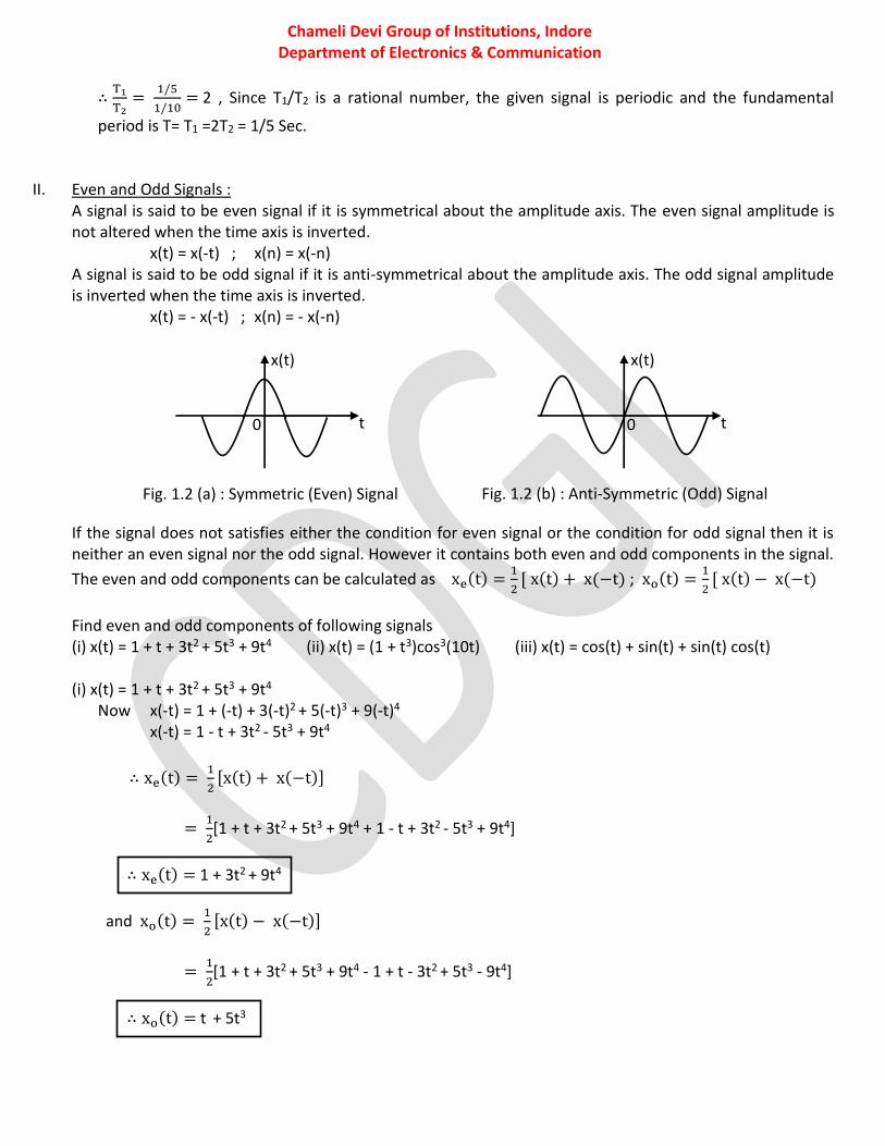
II. Even and Odd Signals : A signal is said to be even signal if it is symmetrical about the amplitude axis. The even signal amplitude is not altered when the time axis is inverted. x(t) = x(-t) ; x(n) = x(-n) A signal is said to be odd signal if it is anti-symmetrical about the amplitude axis. The odd signal amplitude is inverted when the time axis is inverted. x(t) = - x(-t) ; x(n) = - x(-n)

If the signal does not satisfies either the condition for even signal or the condition for odd signal then it is neither an even signal nor the odd signal. However it contains both even and odd components in the signal.

The even and odd components can be calculated as xe(t) =1

2[ x(t) + x(−t) ; xo(t) =

1

2[ x(t) − x(−t)

Find even and odd components of following signals (i) x(t) = 1 + t + 3t2 + 5t3 + 9t4 (ii) x(t) = (1 + t3)cos3(10t) (iii) x(t) = cos(t) + sin(t) + sin(t) cos(t) (i) x(t) = 1 + t + 3t2 + 5t3 + 9t4

Now x(-t) = 1 + (-t) + 3(-t)2 + 5(-t)3 + 9(-t)4

x(-t) = 1 - t + 3t2 - 5t3 + 9t4

∴ xe(t) = 1

2[x(t) + x(−t)]

= 1

2[1 + t + 3t2 + 5t3 + 9t4 + 1 - t + 3t2 - 5t3 + 9t4]

∴ xe(t) = 1 + 3t2 + 9t4

and xo(t) = 1

2[x(t) − x(−t)]

= 1

2[1 + t + 3t2 + 5t3 + 9t4 - 1 + t - 3t2 + 5t3 - 9t4]

∴ xo(t) = t + 5t3

Fig. 1.2 (a) : Symmetric (Even) Signal Signal

Fig. 1.2 (b) : Anti-Symmetric (Odd) Signal Signal

t

x(t)

0 t

x(t)

0


(ii) x(t) = (1 + t3)cos3(10t)

Now x(t) = (1 + t3)(3

4cos(10t) +

1

4cos(30t))

∴ x(−t) = (1 + (−t)3)(3

4cos(−10t) +

1

4cos(−30t))

x(−t) = (1 − t3)(3

4cos(10t) +

1

4cos(30t)

To find the even and odd components, consider the equation

xe(t) = 1

2[x(t) + x(−t)]

xe(t) = 1

2[(1 + t3)(

3

4cos(10t) +

1

4cos(30t)] + [(1 − t3)(

3

4cos(10t) +

1

4cos(30t))]

∴ xe(t) = (3

4cos(10t) +

1

4cos(30t))

and

xo(t) = 1

2[x(t) − x(−t)]

xo(t) = 1

2[(1 + t3) (

3

4cos(10t) +

1

4cos(30t)] − [(1 − t3)(

3

4cos(10t) +

1

4cos(30t))]

∴ xo(t) = t3(3

4cos(10t) +

1

4cos(30t))

(iii) x(t) = cos(t) + sin(t) + sin(t) cos(t)

Now x(-t) = cos(-t) + sin(-t) + sin(-t) cos(-t)

x(-t) = cos(t) - sin(t) - sin(t) cos(t)

∴ xe(t) = 1

2[x(t) + x(−t)]

= 1

2[cos(t) + sin(t) + sin(t) cos(t) + cos(t) - sin(t) - sin(t) cos(t)]

∴ xe(t) = cos(t)

and xo(t) = 1

2[x(t) − x(−t)]

= 1

2[cos(t) + sin(t) + sin(t) cos(t) - cos(t) + sin(t) + sin(t) cos(t)]

∴ xo(t) = sin(t) cos(t) + cos(t)

III. Energy and Power Signals : The signal which has finite energy and zero average power is called as energy signal. If x(t) has 0 < E < ∞ and P = 0 , then it is a energy signal, where E is the energy and P is the average power of signal x(t).

The signal which has finite average power and infinite energy is called as power signal.


If x(t) has 0 < P < ∞ and E = ∞ , then it is a power signal, where E is the energy and P is the average power of signal x(t). If the signal does not satisfies either the condition for energy signal or the condition for power signal then it is neither an energy signal nor the power signal. Energy of Signal: For real CT signal, energy is calculated as

E = ∫ x2(t)dt∞

−∞

For complex valued CT signal, energy is calculated as

E = ∫ |x(t)|2dt∞

−∞

For real DT signal, energy is calculated as

E = ∑ x(n)2∞

n=−∞

For complex valued DT signal, energy is calculated as

E = ∑ |x(n)|2∞

n=−∞

Power of Signal: For real CT signal, average power is calculated as

P = limT→∞

1

T ∫ x2(t)dt

∞

−∞

For complex valued CT signal, average power is calculated as

P = limT→∞

1

T ∫ |x(t)|2dt∞

−∞

For real DT signal, average power is calculated as

P = limN→∞

1

N ∑ x(n)2∞

n=−∞

For complex valued DT signal, average power is calculated as

P = limN→∞

1

N∑ |x(n)|2∞

n=−∞

Comparison of Energy Signal & Power Signal

Sl. No. Energy Signal Power Signal

1 Total normalized energy is finite and non zero

The normalized average power is finite and non zero

2 Non periodic signals are energy signals Periodical signals are power signals

3 Power of energy signal is zero Energy of power signal is infinite

Example : (i) Prove the following (a) The power of the energy signal is zero over infinite time (b) The energy of the power signal is infinite over infinite time Solution : (a) Power of the energy signal

Let x(t) be an energy signal


∴ Power P = limT→∞

1

2T∫ |x(t)|2dtT

−T

= limT→∞

1

2T[ limT→∞

∫ |x(t)|2dtT

−T

]

P = limT→∞

1

2T∫ |x(t)|2dt∞

−∞

= limT→∞

1

2T[E] Since E = ∫ |x(t)|2dt

∞

−∞

∴ P = 1

2∞[E] = 0 X E = 0 Thus, the power of the energy signal is zero over infinite time.

(b) Energy of the power signal

Let x(t) be the power signal

∴ Energy E = ∫ |x(t)|2dt∞

−∞

Consider the limits of integration as –T to T and take limit T tends to . this will not change the meaning of above equation

∴ E = limT→∞

∫ |x(t)|2dtT

−T

= limT→∞

[2T1

2T∫ |x(t)|2dtT

−T

]

∴ E = limT→∞

2T [ limT→∞

1

2T∫ |x(t)|2dtT

−T

] = limT→∞

2TP

∴ E = ∞ Thus, the energy of the power signal is infinite over infinite time. Example : (ii) Sketch the given signal x(t) = e-a|t| for a > 0. Also determine whether the signal is a power signal or energy signal or neither. Solution : The given signal is x(t) = e-a|t| for a > 0 It can be expressed as

x(t) = e−at for t > 0eat for t < 0

The sketch of this signal is shown in Fig. (a)

The energy of the signal is expressed as

Energy E = ∫ |x(t)|2dt∞

−∞

= ∫ e−2a|t|dt∞

−∞

∴ E = ∫ e−2a(−t)0

−∞

dt + ∫ e−2a(t)dt∞

0

∴ E = ∫ e−2at∞

0

dt + ∫ e−2atdt∞

0

= 2∫ e−2atdt∞

0

∴ E = 2 [e−2at

−2a]0

∞

= −1

a [e−∞ − e0] =

1

a Joules

Since energy is finite, the signal is energy signal.

Example : (iii) The signal x(t) is shown in Fig.(b). Determine whether the signal is a power signal or energy signal or neither. Solution : The given signal x(t) can be expressed as

x(t) = 2 for − 1 ≤ t ≤ 02e−t/2 for t > 0

Fig.(a) : Waveforms for Example (ii)

t 0

x(t) = e –a|t|

e –at e at


The energy of the signal is expressed as

Energy E = ∫ |x(t)|2dt∞

−∞

∴ E = ∫ 220

−1

dt + ∫ [2e−(t/2)]2dt∞

0

∴ E = ∫ 40

−1

dt + ∫ 4e−tdt∞

0

∴ E = 4[t]−10 + 4 [

e−t

−1]0

∞

= 4 − 4 [e−∞ − e0] = 4 + 4 = 8 Joules


Example : (iv) The signal x(t) is shown in Fig.(c). Determine whether the signal is a power signal or energy signal or neither. Solution : The given signal x(t) is a periodic signal with period from -1 to 1 (T=2) , can be expressed as

x(t) = t for − 1 ≤ t ≤ 1 Since the signal is periodic, it is a power signal and the average power can be calculated.

The average power of the signal is expressed as

Power P = limT→∞

1

T∫ |x(t)|2dtT/2

−T/2

∴ p =1

2∫ |x(t)|2dtT/2

−T/2

= 1

2∫ t2dt1

−1

∴ P =1

2[t3

3]−1

1

=1

6 .2 =

1

3 Watts


IV. Deterministic and Random Signals A signal which has regular pattern and can be completely represented by mathematical equation at any time is call deterministic signal. i.e., sine wave, exponential signal, square wave and triangular wave etc. A signal which has uncertainty about its occurrence is called random signal. A random signal cannot be represented by mathematical equation. i.e., noise is a random signal

Elementary Signals : (i) Unit Step Signal : The unit step signal has a constant amplitude of unity for t ≥ 0 and zero for negative

values of t.

The mathematical expression for CT unit step signal : u(t) = 1 for t ≥ 0 0 for t < 0

Fig.(c) : Waveforms for Example (iv)

t 0

x(t) = e –a|t|

-1 1 2 3 4 -2

1

-1

Fig.(b) : Waveforms for Example (iii)

t 0

x(t)

2e –t/2

-1 1 2 3 4


The mathematical expression for DT unit step signal : u(n) = 1 for n ≥ 0 0 for n < 0

(ii) Unit Impulse Signal: This signal is most widely used elementary signal in the analysis of systems. It is also

called Dirac delta signal. It is defined as

∫ δ(t)dt = 1∞

−∞

and δ(t) = 0 for t ≠ 0 δ(t)

δ(t)i.e., δ(t) = 1 for t = 00 for t ≠ 0

(iii) Unit Ramp Signal: The unit ramp signal r(t) is that signal which starts at t=0 and increases linearly with time

and is defined as

Continuous time ramp signal r(t) = t for t ≥ 00 for t < 0

or r(t) = t u(t)

Discrete time ramp sequence r(n) = n for n ≥ 00 for n < 0

or r(n) = n u(n)

(iv) Exponential Signal : The continuous-time real exponential signal has general form as x(t) = A eαt , where

both A and α are real number.

t

Fig. 1.4 (a) : CT Ramp Signal

x(t) = r(t)

0

Fig. 1.4 (b) : DT Ramp Signal

n 1 2 3 4

x(t) = r(n)

0

t

x(t) = u(t)

Fig. 1.3 (a) : CT unit Step Signal

0

1

n

x(n) = u(n)

Fig. 1.3 (b) : DT unit Step Signal

0

1

1 2 3 4 5 6

δ(t)

1

t 0

δ(t − a)

1

t 0 a


(v) Sinusoidal Signal: The CT sinusoidal signal has general form as x(t) = A sin (ωt+φ)

Relationships between the signals:

Relation between unit step and unit ramp signal: The unit ramp signal is defined as,

r(t) = t for t ≥ 0 0 for t < 0

Differentiating r(t) with respect to t,

d r(t)

dt=

d (t)

dt for t ≥ 0

0 for t < 0

= 1 for t ≥ 0 0 for t < 0

∴ u(t) =d r(t)

dt

The unit step signal is defined as,

u(t) = 1 for t ≥ 0 0 for t < 0

Integrating u(t) with respect to t,

∫u(t) dt = ∫1dt = t

∴ r(t) = ∫u(t) dt

T0

t

x(t)

Fig. 1.6: CT Sinusoidal Signal

0

t

x(t)

Fig. 1.5: CT Exponential Signal

0 t

x(t)

0

A A

t

x(t)

0

A

x(t) = A eαt for α =0 x(t) = A eαt for α >0 x(t) = A eαt for α <0


Signal Operations and Properties: Following are the operations performed on the signals; (i) Time Shifting (Delay / Advance): The signal can be delayed or advanced by a constant time factor. The signal

x(t) is time delayed if the time factor is having negative value. The signal x(t) is time advanced if the time factor is having positive value. i.e., x(t) is right shifted if it is represented as x(t-2) and left shifted if it is represented as x(t+2). The Fig. shows the time shifting operations.

(ii) Time Folding: Time folding is also called as time reversal of signal x(t) and is denoted by x(-t). The signal x(-t)

is obtained by replacing t with –t in the given x(t).

(a) : CT unit Step Signal

t

x(t) = u(t)

0

1

Fig. 1.8: Time Shifting Operation

n

x(n) = u(n)

0

1

1 2 3 4 5 6

0 t

x(t) = u(t-2)

1

2

t

x(t) = u(t+2)

0

1

-2

n

x(n) = u(n-2)

0

1

1 2 3 4 5 6

n

x(n) = u(n+2)

0

1

1 2 3 4 5 6 -1 -2

Delaying or right shift

Advancing or left shift

(b) : DT unit Step Signal


(iii) Time Scaling (Compression / Expansion): The time scaling may be compression or expansion of time x(t). It is

expressed as y(t) = x(at) where a is the scaling factor. (iv) Amplitude Scaling: The amplitude scaling of the CT signal x(t) is represented as y(t) = A x(t) (v) Signal Addition : The two or more CT signals can be added. The value of new signal is obtained by adding

the value of each signal at every instant of time. Subtraction of one signal from other can also be performed in the similar way.

(vi) Signal Multiplication: The two signal can be multiplied in its continuous time domain. The value of new signal is obtained by multiplying the two signal values at every instant of time.

Signal Sampling: Signal sampling is a process through which the continuous time signal can be represented into discrete time signal. The continuous time signal x(t) is sampled at a regular interval of nT and the x(nT) is called the sampled sequence of x(t). Sampling Theorem: The sampling theorem states that “A band limited signal x(t) with X(ω)=0 for |ω|≥ωm can be represented into and uniquely determined from its samples x(nT) if the sampling frequency fs ≥2fm, where fm is the highest frequency component present in it”. That is, for signal recovery, the sampling frequency must be atleast twice the highest frequency present in the signal.

t

x(t) = u(t)

0

1

Fig. 1.9: Time Folding Operation

n

x(n) = u(n)

0

1

1 2 3 4 5 6

0 t

x(-t) = u(-t)

1

(b) : DT unit Step Signal

x(-n) = u(-n)

n 0

1

-5 -4 -3 -2 -1

(a) : CT unit Step Signal


Example : Sketch the following signals

(a) x(t) = 2u(t+2) – 2u(t-3) (b) x(t) = u(t+4) u(-t+4) (c) x(t) = r(-t) u(t+2) (c) x(t) = r(t) – r(t-1) – r(t-3) + r(t-4)

Solution: (a) Given x(t) = 2u(t+2) – 2u(t-3)

Consider the elementary signal u(t).

The signal 2u(t+2) is obtained by shifting u(t) to the left by 2 units and multiplying by 2

The signal -2u(t-3) is obtained by shifting u(t) to the right by 3 units and multiplying by -2

The signal x(t) is obtained by adding 2u(t+2) and – 2u(t-3)

The sketch of all the signals are shown in Fig. (a).

Solution: (b) Given x(t) = u(t+4) u(-t+4)

t

t

0

2

t 0

u(t)

-2 3

Fig.(a) : Waveforms for Example (a)

1

2u(t+2) – 2u(t-3)

0

-2

-2u(t-3)

3

t 0

2 2u(t+2)

-2


Consider the elementary signal u(t).

The signal u(t+4) is obtained by shifting u(t) to the left by 4 units

The signal u(-t+4) is obtained by reversing u(t) and then shifting u(-t) to the right by 4 units

The signal x(t) is obtained by multiplying u(t+4) and u(-t+4)

The sketch of all the signals are shown in Fig. (b).

Solution: (c) Given x(t) = r(-t) u(t+2)

Consider the elementary signals u(t) and r(t).

The signal u(t+2) is obtained by shifting u(t) to the left by 2 units

The signal r(-t) is obtained by time reversing r(t)

The signal x(t) is obtained by multiplying r(-t) and u(t+2)

The sketch of all the signals are shown in Fig. (c).

(a) Solution: (d) Given x(t) = r(t) – r(t-1) – r(t-3) + r(t-4)

Consider the elementary signals r(t).

The signal r(t-1) is

t

t

t

t

0

0

0

0

2

2

1 1

u(t) u(t+2)

r(-t)

-2

-2 4

r(-t) u(t+2)

Fig.(c) : Waveforms for Example (c)

t 0

2 r(t)

2 -2

t

t

t

t

0

0

0

0

1

1

1 1

u(t) u(t+4)

u(-t+4)

4

-4

-4 4

u(-t+4) u(t+4)

t 0

1

u(-t)

Fig.(b) : Waveforms for Example (b)


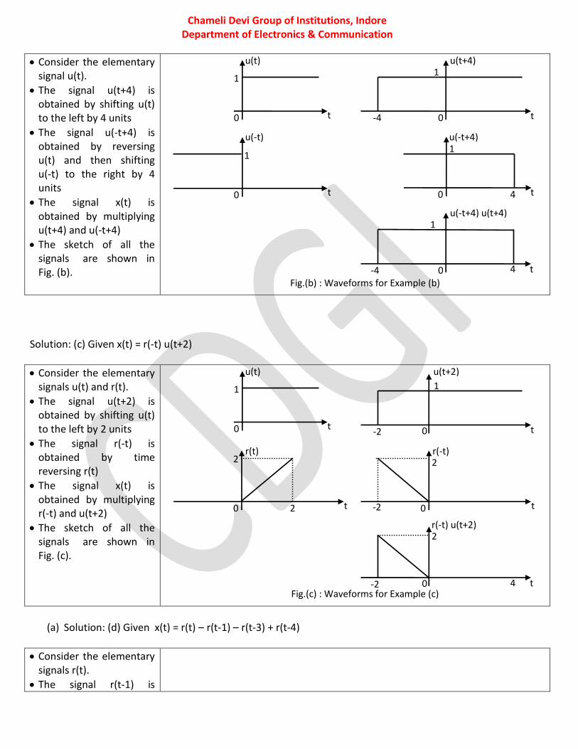
obtained by shifting r(t) to the right by 1 unit with slope -1

Similarly the signal r(t-3) is obtained by shifting r(t) to the right by 3 units with slope -1 and the signal r(t-4) is obtained by shifting r(t) to the right by 4 units with slope 1

The signal x(t) is obtained by adding r(-t), -r(t-1), -r(t-3) and r(t+4)

The sketch of all the signals are shown in Fig. (d).

Basic System Properties : (I) Causality (II) Time Invariant & Variant (III) Linearity (IV) Stability (V) Static & Dynamic (VI) Invertible & Non-Invertible (I) Causal and Non-causal System : A system is said to be causal if its output y(t) at any arbitrary time t0

depends only on the values of its input x(t) for t ≤ t0. In the causal system the output does not begin before the input signal is applied. If the independent variable represents time, a system must be causal in order to be physically realizable. Noncausal systems can sometimes be useful in practice, however, as the independent variable need not always represent time.

Example : Determine whether the following systems are causal or non-causal

(i) y(t) = 0.2x(t) – x(t-1) (ii) y(t) = 0.8x(t-1) (iii) y(n) = x(n-1) (iv) y(t) = x(t+1) (v) y(n-2) = x(n) (vi) y(n) = x(n) –x(n+1) Solution:

(i) Given that y(t) = 0.2x(t) – x(t-1) In the above equation put t=0 then y(0) = 0.2x(0) – x(-1) put t=1 then y(1) = 0.2x(1) – x(0) Since the output y(t) depends on the present and the past input values of x(t), the system is causal

(ii) Given that y(t) = 0.8x(t-1) In the above equation put t=0 then y(0) = 0.8 x(-1) put t=1 then y(1) = 0.8 x(0)

t t 0 0

1

r(t)- r(t-1)

Fig.(d) : Waveforms for Example (d)

1 3 4

r(t)

-r(t-1) -r(t-3)

r(t-4)

t 0

1

r(t)- r(t-1)-r(t-3)

t 0

1

r(t)- r(t-1)-r(t-3)+r(t-4)


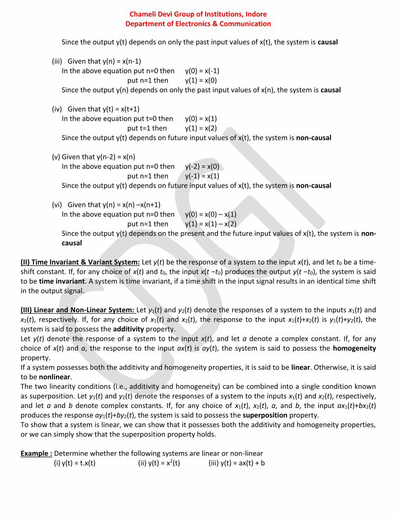
Since the output y(t) depends on only the past input values of x(t), the system is causal

(iii) Given that y(n) = x(n-1) In the above equation put n=0 then y(0) = x(-1) put n=1 then y(1) = x(0) Since the output y(n) depends on only the past input values of x(n), the system is causal

(iv) Given that y(t) = x(t+1) In the above equation put t=0 then y(0) = x(1) put t=1 then y(1) = x(2) Since the output y(t) depends on future input values of x(t), the system is non-causal

(v) Given that y(n-2) = x(n) In the above equation put n=0 then y(-2) = x(0) put n=1 then y(-1) = x(1) Since the output y(t) depends on future input values of x(t), the system is non-causal

(vi) Given that y(n) = x(n) –x(n+1) In the above equation put n=0 then y(0) = x(0) – x(1) put n=1 then y(1) = x(1) – x(2) Since the output y(t) depends on the present and the future input values of x(t), the system is non-causal

(II) Time Invariant & Variant System: Let y(t) be the response of a system to the input x(t), and let t0 be a time-shift constant. If, for any choice of x(t) and t0, the input x(t −t0) produces the output y(t −t0), the system is said to be time invariant. A system is time invariant, if a time shift in the input signal results in an identical time shift in the output signal. (III) Linear and Non-Linear System: Let y1(t) and y2(t) denote the responses of a system to the inputs x1(t) and x2(t), respectively. If, for any choice of x1(t) and x2(t), the response to the input x1(t)+x2(t) is y1(t)+y2(t), the system is said to possess the additivity property. Let y(t) denote the response of a system to the input x(t), and let a denote a complex constant. If, for any choice of x(t) and a, the response to the input ax(t) is ay(t), the system is said to possess the homogeneity property. If a system possesses both the additivity and homogeneity properties, it is said to be linear. Otherwise, it is said to be nonlinear. The two linearity conditions (i.e., additivity and homogeneity) can be combined into a single condition known as superposition. Let y1(t) and y2(t) denote the responses of a system to the inputs x1(t) and x2(t), respectively, and let a and b denote complex constants. If, for any choice of x1(t), x2(t), a, and b, the input ax1(t)+bx2(t) produces the response ay1(t)+by2(t), the system is said to possess the superposition property. To show that a system is linear, we can show that it possesses both the additivity and homogeneity properties, or we can simply show that the superposition property holds. Example : Determine whether the following systems are linear or non-linear

(i) y(t) = t.x(t) (ii) y(t) = x2(t) (iii) y(t) = ax(t) + b


Solution: (i) Given that y(t) = t.x(t)

Let y1(t) = tx1(t) and y2(t) = tx2(t) Now, the linear combination of the two outputs will be y3(t) = a1 y1(t) + a2y2(t) = a1 tx1(t) + a2tx2(t) Also the response to the linear combination of input will be y4(t) =f[a1x1(t) + a2x2(t)] = t[a1x1(t) + a2x2(t)] y4(t) = a1t x1(t) + a2t x2(t) Since the output y3(t) = y4(t), the system is linear system.

(ii) Given that y(t) = x2(t)

Let y1(t) = x12(t) and y2(t) = x2

2(t) Now, the linear combination of the two outputs will be y3(t) = a1 y1(t) + a2y2(t) = a1 x1

2(t) + a2 x22(t)

Also the response to the linear combination of input will be y4(t) =f[a1x1(t) + a2x2(t)] = [a1x1(t) + a2x2(t)]2 y4(t) = a1 x1

2(t) + a2 x22(t) + 2a1 a2 x1(t) x2(t)

Since the output y3(t) ≠ y4(t), the system is not a linear system.

(iii) Given that y(t) = ax(t) + b

Let y1(t) = ax1(t)+b and y2(t) = ax2(t)+b Now, the linear combination of the two outputs will be y3(t) = a1 y1(t) + a2y2(t) = a1(ax1(t)+b) + a2 (ax2(t)+b) Also the response to the linear combination of input will be y4(t) =f[a1x1(t) + a2x2(t)] = a[a1x1(t) + a2x2(t)] + b Since the output y3(t) ≠ y4(t), the system is not a linear system.

(IV) Memory and Memory-less System: A system is said to have memory if its output y(t) at any arbitrary time t0 depends on the value of its input x(t) at any time other than t = t0. If a system does not have memory, it is said to be memory less. (V) Invertible and Non-invertible System: A system is said to be invertible if its input x(t) can always be uniquely determined from its output y(t). From this definition, it follows that an invertible system will always produce distinct outputs from any two distinct inputs. If a system is invertible, this is most easily demonstrated by finding the inverse system. If a system is not invertible, often the easiest way to prove this is to show that two distinct inputs result in identical outputs. (VI) Stability : The bounded-input bounded-output (BIBO) stability is most commonly defined in system analysis. A system having the input x(t) and output y(t) is BIBO stable if, a bounded input produces a bounded output.


Unit-II : Response of Continuous Time–LTI System: Impulse response and convolution integral, properties of convolution, signal responses to CT-LTI system. Impulse response and convolution integral: Convolution is a mathematical operation which is used to find the response of LTI system. In the LTI system analysis it relates the impulse response of the system and input signal to the output. Any signal x(t) can be represented as a continuous sum of impulse signals. The response y(t) can then be represented as sum of responses of various impulse components. The impulse response is denoted as h(t) = T[δ(t)] Any arbitrary signal can be represented as


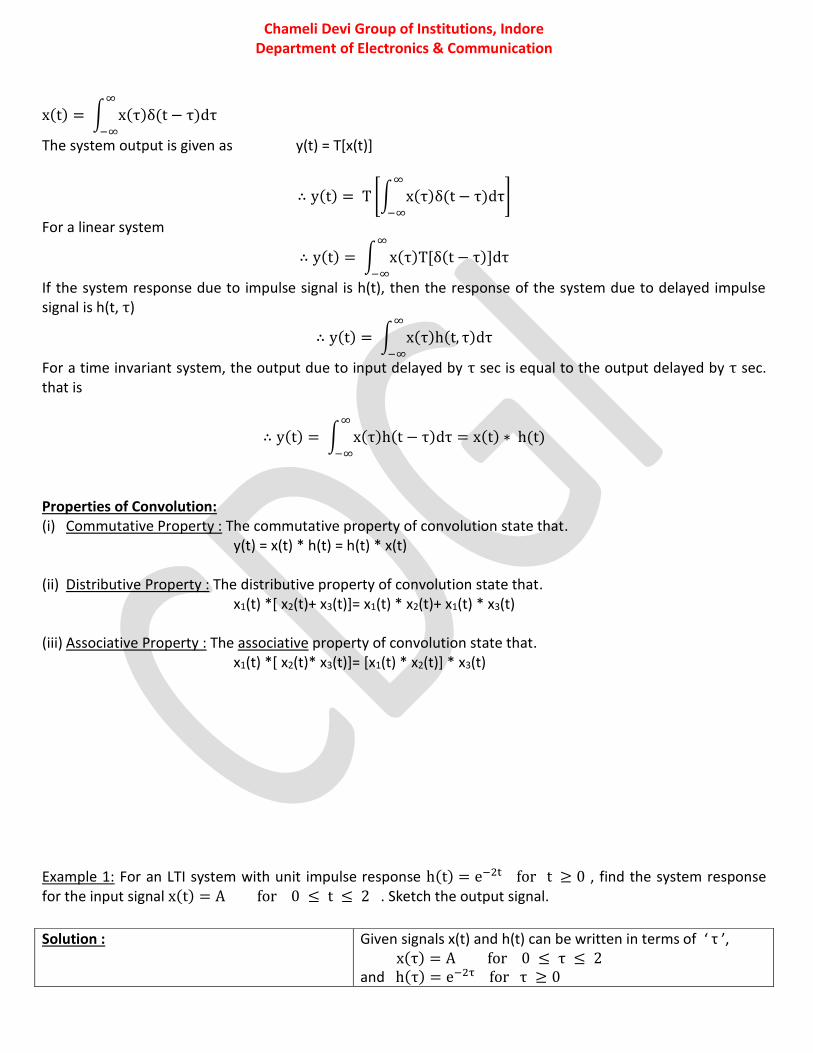
x(t) = ∫ x(τ)δ(t − τ)dτ∞

−∞

The system output is given as y(t) = T[x(t)]

∴ y(t) = T [∫ x(τ)δ(t − τ)dτ∞

−∞

]

For a linear system

∴ y(t) = ∫ x(τ)T[δ(t − τ)]dτ∞

−∞

If the system response due to impulse signal is h(t), then the response of the system due to delayed impulse signal is h(t, τ)

∴ y(t) = ∫ x(τ)h(t, τ)dτ∞

−∞

For a time invariant system, the output due to input delayed by τ sec is equal to the output delayed by τ sec. that is

∴ y(t) = ∫ x(τ)h(t − τ)dτ∞

−∞

= x(t) ∗ h(t)

Properties of Convolution: (i) Commutative Property : The commutative property of convolution state that.

y(t) = x(t) * h(t) = h(t) * x(t)

(ii) Distributive Property : The distributive property of convolution state that. x1(t) *[ x2(t)+ x3(t)]= x1(t) * x2(t)+ x1(t) * x3(t)

(iii) Associative Property : The associative property of convolution state that.

x1(t) *[ x2(t)* x3(t)]= [x1(t) * x2(t)] * x3(t)

Example 1: For an LTI system with unit impulse response h(t) = e−2t for t ≥ 0 , find the system response for the input signal x(t) = A for 0 ≤ t ≤ 2 . Sketch the output signal.

Solution : Given signals x(t) and h(t) can be written in terms of ‘ τ ’, x(τ) = A for 0 ≤ τ ≤ 2 and h(τ) = e−2τ for τ ≥ 0


Example 2: Consider x(t) = 2 for 1 ≤ t ≤ 2

Now h(t − τ) = e−2(t−τ) for t − τ ≥ 0 The signals x(τ) and h(t − τ) are shown in Fig. . The output of the system is given by the linear convolution as,

y(t) = ∫ x(τ) h(t − τ)dτ∞

−∞

The integral is non Zero for overlap between Case – I : For 0 ≤ t ≤ 2 In this case, there will be partial overlap between x(τ) and h(t − τ) as shown in the Fig.

∴ y(t) = ∫ x(τ) h(t − τ)dτt

0

∴ y(t) = ∫ A e−2(t−τ)dτt

0

= Ae−2t ∫ e2τdτt

0

= Ae−2t 1

2[e2τ]0

t = Ae−2t 1

2(e2t − 1)

∴ y(t) = A

2(1 − e−2t)

Case – I : For t > 2 In this case, there will be complete overlap from 0 to 2 as shown in the Fig.

∴ y(t) = ∫ x(τ) h(t − τ)dτ2

0

= ∫ A e−2(t−τ)dτ2

0

= Ae−2t ∫ e2τdτ2

0

∴ y(t) = Ae−2t 1

2[e2τ]0

2 = 26.8Ae−2t

Thus y(t) =

0 for t < 0A

2(1 − e−2t) for 0 ≤ t ≤ 2

26.8Ae−2t for t < 0

x(τ)

τ 0 2 1

A

h(τ)

τ 0

h(-τ)

τ 0

h(t-τ)

τ 0 t

0 ≤ t ≤ 2

h(t-τ)

τ 0 t

t > 2

2 1

Fig. :Evaluation of Convolution Integral

0.49A

y(t)

t 0 2 1

Fig. :Sketch of output Signal


and h(t) = 1 for 0 ≤ t ≤ 3 , find x(t) * h(t)

Solution :

Given signals x(t) and h(t) can be written in terms of ‘ τ ’, x(τ) = 2 for 1 ≤ τ ≤ 2 and h(τ) = 1 for 0 ≤ τ ≤ 3 The signals x(τ) and h(t − τ) are shown in Fig.2a. The output of the system is given by the linear convolution as,

y(t) = ∫ x(τ) h(t − τ)dτ∞

−∞

The integral is non Zero for overlap between x(τ) and h(t − τ) Case – I : For 0 ≤ t < 1 In this case, there is no overlap between x(τ) and h(t − τ) as shown in the Fig. ∴ y(t) = 0 Case – II : For 1 ≤ t ≤ 2 In this case, there is partial overlap between x(τ) and h(t − τ) as shown in the Fig. The limits of integration are 1 to t

∴ y(t) = ∫ x(τ) h(t − τ)dτt

1

∴ y(t) = ∫ 2.1. dτt

1= 2 ∫ dτ = 2 [τ]1

t = 2t t

1

∴ y(t) = 2t Case – III : For 2 ≤ t ≤ 4 In this case, there is complete overlap between x(τ) and h(t − τ) as shown in the Fig. The limits of integration are 1 to 2

∴ y(t) = ∫ x(τ) h(t − τ)dτ2

1

∴ y(t) = ∫ 2.1. dτ2

1= 2 ∫ dτ = 2 [τ]1

2 = 2 2

1

∴ y(t) = 2 Case – IV : For 4 ≤ t ≤ 5 In this case, there is partial overlap between x(τ) and h(t − τ) as shown in the Fig. The limits of integration are t-3 to 2

∴ y(t) = ∫ x(τ) h(t − τ)dτ2

t−3

0 ≤ t < 1

Fig.2a :Evaluation of Convolution Integral

x(τ)

τ 0 2 1

h(τ)

τ 0

2

3

τ 0 -3

1

1 h(-τ)

τ 0 t-3

1 h(t-τ)

t

0 t-3

1 h(t-τ)

t

1 ≤ t ≤ 2

τ 1

0 t-3

1

t 1 τ

2 ≤ t ≤ 4

2

0

1

1 τ 2

4 ≤ t ≤ 5

t-3 t

h(t-τ)

h(t-τ)

0

1

1 2

t > 5

t-3 t

h(t-τ)

τ


Example 3: Consider x(t) = u(t + 2) and h(t) = u(t − 3) , find x(t) * h(t)

∴ y(t) = ∫ 2.1. dτ2t

t−3

= 2 ∫ dτ = 2 [τ]t−32 = 2(1 − t)

2t

t−3

∴ y(t) = 2(1 − t) Case – V : For t > 5 In this case, there is no overlap between x(τ) and h(t − τ) as shown in the Fig. ∴ y(t) = 0

y(t)

0 2 1

Fig.2b :Sketch of output Signal

t 3 4 5

2


Example 4: Obtain the convolution of the following two signals

Solution :

Given signals x(t) and h(t) can be written in terms of ‘ τ ’, x(τ) = u(τ + 2) and h(τ) = u(τ − 3) The signals x(τ) and h(t − τ) are shown in Fig.3a. The output of the system is given by the linear convolution as,

y(t) = ∫ x(τ) h(t − τ)dτ∞

−∞

The integral is non Zero for overlap between x(τ) and h(t − τ) Case – I : For t < 1 In this case, there is no overlap between x(τ) and h(t − τ) as shown in the Fig. ∴ y(t) = 0 Case – II : For t ≥ 1 In this case, there is overlap between x(τ) and h(t − τ) as shown in the Fig. The limits of integration are -2 to t-3

∴ y(t) = ∫ x(τ) h(t − τ)dτt−3

−2

∴ y(t) = ∫ 1.1. dτt−3

−2

= ∫ dτ = [τ]−2t−3 = (t − 3 + 2)

t

1

∴ y(t) = t − 1


x(τ)= u(τ+2)

τ 0 -2

1

τ

t < 1

t

h(τ)= u(τ-3)

τ 0 3

1

h(τ)= u(-τ+3)

τ 0

1

-3

h(τ)= u(t-τ+3)

τ 0

1

t-3 -2 t ≥ 1 h(τ)= u(t-τ+3)

0

1

t-3 -2

0 2 1


3 4 5

1 y(t)=t-1


Solution :

Given signals x(t) and h(t) can be written in terms of ‘ τ ’, The signals x(τ) and h(t − τ) are shown in Fig.4a. The output of the system is given by the linear convolution as,

y(t) = ∫ x(τ) h(t − τ)dτ∞

−∞

The integral is non Zero for overlap between x(τ) and h(t − τ) Case – I : For t < -3 In this case, there is no overlap between x(τ) and h(t − τ) as shown in the Fig. ∴ y(t) = 0 Case – II : For -3 ≤ t ≤ 0 In this case, there is overlap between x(τ) and h(t − τ) as shown in the Fig. The limits of integration are -3 to t

∴ y(t) = ∫ x(τ) h(t − τ)dτt

−3

∴ y(t) = ∫ 1.2. dτt

−3

= 2∫ dτ = 2[τ]−3t = 2(t + 3)

t

−3

∴ y(t) = 2( t + 3)

Case – III : For 0 ≤ t ≤ 3 In this case, there is overlap between x(τ) and h(t − τ) as shown in the Fig. The limits of integration are t-3 to t

∴ y(t) = ∫ x(τ) h(t − τ)dτt

t−3

∴ y(t) = ∫ 1.2. dτt

t−3

= 2∫ dτ = 2[τ]t−3t = 2(t − t + 3)

t

t−3

∴ y(t) = 6

Case – IV : For 3 ≤ t ≤ 6 In this case, there is overlap between x(τ) and h(t − τ) as shown in the Fig. The limits of integration are t-3 to 3

∴ y(t) = ∫ x(τ) h(t − τ)dτ3

t−3

∴ y(t) = ∫ 1.2. dτ3

t−3

= 2∫ dτ = 2[τ]t−33 = 2(3 − t + 3)

3

t−3

∴ y(t) = 2(−t + 6)

Case – V : For t >6 In this case, there is no overlap between x(τ) and


x(τ)

τ 0 -3

1

t

h(τ)

τ 0 3

2

-3 2 -2


3 4 5

6

y(t)

3

h(-τ)

τ 0 -3

2

h(t-τ)

τ 0 t-3

2

t -3 3

-3 ≤ t ≤ 0

h(t-τ)

τ 0 t-3

2

t -3 3

0 ≤ t ≤ 3

1

1

h(t-τ)

τ 0 t-3

2

t -3 3

3 ≤ t ≤ 6

1

-1 0 1 6


x(t) = 1 for − 3 ≤ t ≤ 30 else where

and h(t) = 2 for 0 ≤ t ≤ 30 else where

Example 5: Obtain the convolution of the following two signals shown in Fig.5a.

h(t − τ) as shown in the Fig. ∴ y(t) = 0


Solution :

Given signals x(t) and h(t) can be written in terms of ‘ τ ’, The signals x(τ) and h(t − τ) are shown in Fig.5a. The output of the system is given by the linear convolution as,

y(t) = ∫ x(τ) h(t − τ)dτ∞

−∞

The integral is non Zero for overlap between x(τ) and h(t − τ) Case – I : For t < 0 In this case, there is no overlap between x(τ) and h(t − τ) as shown in the Fig. ∴ y(t) = 0 Case – II : For 0 ≤ t ≤ 2 In this case, there is overlap between x(τ) and h(t − τ) as shown in the Fig. The limits of integration are 0 to t

∴ y(t) = ∫ x(τ) h(t − τ)dτt

0

∴ y(t) = ∫ τ. 2. dτt

0

= 2∫ τdτ = 2 [τ2

2]0

t

= t2 t

0

∴ y(t) = t2

Case – III : For 2 ≤ t ≤ 4 In this case, there is overlap between x(τ) and h(t − τ) as shown in the Fig. The limits of integration are t-2 to t

∴ y(t) = ∫ x(τ) h(t − τ)dτt

t−2

∴ y(t) = ∫ τ. 2. dτ + ∫ (4 − τ).2. dτt

2

2

t−2

∴ y(t) = 2 [τ2

2]t−2

2

+ 2 [(4 − τ)2

2]2

t

∴ y(t) = (4 − (t − 2)2) + ((4 − t)2 − 4) ∴ y(t) = 12 − 4t Case – IV : For 4 ≤ t ≤ 6 In this case, there is overlap between x(τ) and h(t − τ) as shown in the Fig. The limits of integration are t-2 to 4

∴ y(t) = ∫ x(τ) h(t − τ)dτ4

t−2

∴ y(t) = ∫ (4 − τ).2. dτ4

t−2

= 2 [(4 − τ)2

2]t−2

4

∴ y(t) = −(6 − t)2

Case – V : For t >6


x(τ)

τ 0

2

h(τ)

τ 0 2

2

0 ≤ t ≤ 2

2 ≤ t ≤ 4

4 ≤ t ≤ 6

4 2

h(-τ)

τ 0 -2

2

h(t-τ)

τ 0 t-2

2

4 2 t

h(t-τ)

τ 0 t-2

2

4 2 t

h(t-τ)

τ 0 t-2

2

4 2 t


Unit- III : z-Transform: Introduction, ROC of finite duration sequence, ROC of infinite duration sequence, Relation between Discrete time Fourier Transform and z-transform, properties of the ROC, Properties of z-transform, Inverse z-Transform, Analysis of discrete time LTI system using z-Transform, Unilateral z-Transform Introduction: The z-transform of x(n) is denoted by X(z). It is defined as,

In this case, there is no overlap between x(τ) and h(t − τ) as shown in the Fig. ∴ y(t) = 0


X(z) = ∑ x[n]𝑧−𝑛∞

𝑛=−∞

Region of Convergence (ROC): The set of values of z in the z-plane for which the magnitude of X(z) is finite is called the Region of Convergence (ROC). The ROC of X(z) consists of a circle in the z-plane centered about the origin. The Fig.3.1 shows the two possible representation of ROC in z-plane.

Significance of ROC: (i) ROC gives an idea about values of z for which z-transform can be calculated (ii) ROC can be used to test the causality of the system. (iii) ROC can also be used to test the stability of the system. Examples: (1) Determine the z-transform of following sequence

(i) x1(n) = 1,2,3,4,5,0,7 (ii) x2(n) = 1,2,3,4,5,0,7

Re (Z)

Im (Z)

Unit Circle

Region of Convergence (ROC)

Re (Z)

Im (Z)

Unit Circle

Region of Convergence (ROC)

Fig.3.1 : Region of Convergence Plot in Z-Plane

(a): ROC outside Unit Circle (b): ROC inside Unit Circle


Solution: (i) Given that x1(n) = 1,2,3,4,5,0,7 By definition,

X1(z) = ∑ x1[n]z−n

∞

n=−∞

∴ X1(z) = ∑x1[n]z−n

6

n=0

∴ X1(z) = x(0) + x(1)z

−1 + x(2)z−2 + x(3)z−3 + x(4)z−4 + x(5)z−5 + x(6)z−6

X1(z) = 1 + 2z−1 + 3z−2 + 4z−3 + 5z−4 + 7z−6

X1(z) is convergent for all values of z, except z=0. Because X1(z) = ∞ for z=0. Therefore the ROC is entire z=plane

except z=0. (ii) Given that x2(n) = 1,2,3,4,5,0,7 By definition,

X2(z) = ∑ x2[n]z−n

∞

n=−∞

∴ X2(z) = ∑ x2[n]z−n

3

n=−3

∴ X2(z) = x(−3)z

3 + x(−2)z2 + x(−1)z1 + x(0) + x(1)z−1 + x(2)z−2 + x(3)z−3

X1(z) = z3 + 2z2 + 3z1 + 4 + 5z−1 + 7z−3

X2(z) is convergent for all values of z, except z=0 and z=∞. Because X2(z) = ∞ for z=0. Therefore the ROC is entire

z=plane except z=0 and z=∞.


Z-Transform of Unit Step, u(n) We know that u(n) = 1 for n≥0 = 0 otherwise By definition

X(z) = ∑ x(n)z−n∞

n=−∞

Now x(n) = u(n) present from n=0 to ∞

∴ X(z) = ∑u(n)z−n∞

n=0

∴ X(z) = ∑1. z−n∞

n=0

= 1 + 𝑧−1 + 𝑧−2 + 𝑧−3 + 𝑧−4 + ………. = 1 + 𝑧−1 + (𝑧−1)2 + (𝑧−1)3 + (𝑧−1)4 + …… ..

X(z) = 1

1 − 𝑧−1=

𝑧

𝑧 − 1

The above equation converges if |z-1|<1 i.e., ROC is |z| >1. Therefore the ROC is the exterior to the unit circle in the z-plane.

Find Z-transform of given sequence x(n) = -an u(n-1)

Given that x(n) = −an for n ≤ 10 for n ≥ 0

By definition

X(z) = ∑ x(n)z−n∞

n=−∞

The given sequence x(n) exists from -∞ to -1

∴ X(z) = ∑ x(n)z−n−1

n=−∞

= ∑ −anz−n−1

n=−∞

= − ∑ (a−1z)−n−1

n=−∞

= −∑(a−1z)n∞

n=1

= −∑(a−1z)n∞

n=0

+ 1

= −[1 + (a−1𝑧)1 + (a−1𝑧)2 + (a−1𝑧)3+. . . . ] + 1

X(z) = 1 −1

1 − a−1z= 1 − a−1z − 1

1 − a−1z=−a−1z

1 − a−1z

X(z) = z

z − a

Relation between Discrete time Fourier Transform and z-transform

The Z-transform of a discrete sequence x(n) is defined as

X(z) = ∑ x(n)z−n∞

𝑛=−∞

The Fourier transform of a discrete sequence x(n) is defined as

X(ω) = ∑ x[n]e−jωn∞

n=−∞

The X(z) is the unique representation of the sequence x(n) in the complex z-plane. Let z = rejω

∴ X(z) = ∑ x(n)(rejω)−n

∞

𝑛=−∞

= ∑ [x(n)r−n]e−jωn∞

𝑛=−∞

The RHS of the above equation is the Fourier transform of x(n)r-n , ∴ The Z-transform of x(n) is the Fourier transform of x(n)r-n. If r=1, then


∴ X(z) = ∑ x(n)e−jωn∞

𝑛=−∞

= X(ω)

Therefore the Fourier transform of x(n) is same as the Z-transform of x(n) evaluated along the unit circle centered at the origin of the z-plane.

∴ X(ω) = X(z)|z=ejω = ∑ x(n)z−n|z=ejω

∞

n=−∞

= ∑ x(n)e−jωn∞

n=−∞

For X(ω) to exist, the ROC must include the unit circle. Since ROC cannot contain any poles of X(z) all the poles must lie inside the unit circle. Therefore, the Fourier transform can be obtained from Z-transform X(z) for any sequence x(n) if the poles of X(z) are inside the unit circle. Properties of Z – Transform: The Z-transform has different properties which can be used to obtain the z-transform of a given sequence. Any complex sequence z-transform can be determined by using the properties, which makes the z-transform a powerful tool for discrete-time system analysis.

(i) Linearity Property It states that, the Z-transform of a weighted sum of two sequences is equal to the weighted sum of individual Z-transforms.

If x1(n) ZT ↔ X1(z), with ROC = R1

and x2(n) ZT ↔ X2(z), with ROC = R2

then

ax1(n) + bx2(n) ZT↔ aX1(z) + bX2(z), with ROC = R1 ∩ R2

Proof: By definition

Z[x(n)] = X(z) = ∑ x(n)z−n∞

n=−∞

Z[ax1(n) + bx2(n)] = ∑ [ax1(n) + bx2(n)]z−n

∞

n=−∞

= ∑ ax1(n)z−n

∞

n=−∞

+ ∑ bx2(n)z−n

∞

n=−∞

= a ∑ x1(n)z−n

∞

n=−∞

+ b ∑ x2(n)z−n

∞

n=−∞

= aX1(z) + bX2(z) ; ROC = R1 ∩ R2

ax1(n) + bx2(n) ZT↔ aX1(z) + bX2(z)

(ii) Time Shifting Property It states that,

If x(n) ZT ↔ X(z), with ROC = R

and with zero initial conditions

then x(n − m) ZT ↔ z−m X2(z),

with ROC =R except for the possible addition or deletion of the origin or infinity. Proof: By definition

Z[x(n)] = X(z) = ∑ x(n)z−n∞

n=−∞

Z[x(n − m)] = ∑ x(n − m)z−n∞

n=−∞

Put p=n-m in the summation, then n=m+p.

Z[x(n − m)] = ∑ x(p)z−(m+p)∞

p=−∞

Z[x(n − m)] = z−m ∑ x(p)z−p∞

p=−∞

Z[x(n − m)] = z−mX(z)

Z[x(n − m)] ZT↔ z−mX(z)

Z[x(n + m)] ZT↔ zmX(z)


(iii) Multiplication by an Exponential Sequence Property (Scaling Property) It states that,

If x(n) ZT↔ X(z), with ROC = R

then anx(n) ZT↔ X (

z

a) , with ROC = |a|R

where ‘a’ is a complex number Proof: By definition

Z[x(n)] = X(z) = ∑ x(n)z−n∞

n=−∞

Z[anx(n)] = ∑ anx(n)z−n∞

n=−∞

= ∑x(n) (z

a)−n

∞

n=−∞

= X (z

a)

anx(n) ZT↔ X (

z

a)

ejωnx(n) ZT↔ X (

z

ejω)= X(e−jωz)

e−jωnx(n) ZT↔ X (

z

e−jω)= X(ejωz)

(iv) Time Reversal Property It states that,

If x(n) ZT↔ X(z), with ROC = R

then x(−n) ZT↔ X (

1

z) , with ROC =

1

R


Z[x(n)] = X(z) = ∑ x(n)z−n∞

n=−∞

Z[x(−n)] = ∑ x(−n)zn∞

n=−∞

Z[x(−n)] = ∑ x(−n)(z−1)−n∞

n=−∞

∴ Z[x(−n)] = X(z−1)

Sl. No. Time Domain Sequence x(n)

Z-Transform X(z) ROC

1. δ(n) 1 Entire Z-plane

2. u(n) 1

1 − z−1 |z|>1


3. anu(n) 1

1 − az−1 |z|>|a|

4. -anu(-n-1) 1

1 − az−1 |z|<|a|

5. n.anu(n) az−1

(1 − az−1)2 |z|>|a|

6. -n.anu(-n-1) az−1

(1 − az−1)2 |z|<|a|

Inverse z-Transform: Inverse z-transform of X(z) can be obtained by three different methods,

(i) Power Series Expansion (Long Division Method) (ii) Partial Fraction Expansion (iii) Contour Integration (Residue Method)

(i) Power Series Expansion (Long Division Method): Example: Determine the inverse z-transform of the following (i) X(z) = (1/(1-az-1) , ROC |z|>|a| (ii) X(z) = (1/(1-az-1) , ROC |z|<|a|

Thus we have

X(z) = 1

1 − az−1= 1 + az−1 + a2z−2 + a3z−3 +−−−

Taking Inverse z-transform , x(n) = 1,a,a2,a3,-------- x(n) = an u(n)

1-az-1 1 1 - az-1

- +

az-1

az-1 - a2z-2 - +

a2z-2

a2z-2 - a3z-3 - +

a3z-3

a3z-3 - a4z-4 - +

a4z-4 -----

1+az-1+a2z-2+a3z-3+ ------ Solution: (i)


Thus we have

X(z) = 1

1 − az−1= − a−1z − a−2z2 − a−3z3 +−−−

Taking Inverse z-transform , x(n) = ---------------, -a-3,-a-2,-a-1, x(n) = -an u(-n-1) (ii) Partial Fraction Method:

Step - 1 : First convert given X(z) into positive powers of z and then write X(z)

z

Step - 2 : Using partial fraction method, write the equation in terms of summation of poles. Find the constants in the numerator.

Step - 3 : Rewrite the equation in the form of X(z). Step - 4 : Based on the condition of ROC, write the inverse z-transform x(n) of X(z). (iii) Contour Integration (Residue Method: Step-1: Define the function X0(z) which is rational and its denominator is expanded into product of poles. X0(z) = X(z) zn-1 Step-2: (i) For Simple poles, the residue of X0(z) at pole pi is given as,

Resz=pi

= limz=pi(z − pi) X0(z)

(ii) For multiple poles of order m0, the residue of X0(z) can be calculated as,

Resz=pi

= 1

(m − 1)!dm−1

dzm−1(z − pi)X0(z)

z=pi

Step-3: (i) Using residue theorem, calculate x(n), for poles inside the unit circle

x(n) = ∑Resz=pi

N

i=1

X0(z) with n ≥ 0

(ii) Using residue theorem, calculate x(n), for poles outside the unit circle

-az-1 + 1 1 1 – a-1z

- +

a-1z

a-1z - a-2z2 - +

a-2z2

a-2z2 - a-3z3 - +

a-3z3

a-3z3 - a-4z4 - +

a-4z-4 -----

- a-1z - a-2z2 - a-3z3 - ------ Solution: (ii)


x(n) = − ∑Resz=pi

N

i=1

X0(z) with n < 0

Solution of Difference Equations using Z-transform: The difference equations can be easily solved using z-transform. Examples : (1) Given that y(-1) =5 and y(-2)=0, solve the difference equation y(n) - 3y(n-1) – 4y(n-2) = 0 , n ≥ 0. Solution : Consider the given difference equation y(n) - 3y(n-1) – 4y(n-2) = 0 Taking unilateral z-transform of the given difference equation Y(z) – 3 [z-1Y(z) + y(-1)] - 4 [z-2Y(z) + z-1y(-1) + y(-2)] = 0 Put the initial conditions in above equation, we get Y(z) – 3 [z-1Y(z) + 5] - 4 [z-2Y(z) + 5z-1 + 0] = 0 Y(z)[1 – 3z-1 - 4 z-2] - 20z-1 -15 = 0

Y(z) =15 + 20z−1

1 − 3z−1 − 4z−2=z(15z + 20)

z2 − 3z − 4

Y(z)

z=(15z + 20)

z2 − 3z − 4=

(15z + 20)

(z + 1)(z − 4)

Using partial faction method, the above equation can be written as, (15z + 20)

(z + 1)(z − 4)=

A

(z + 1)+

B

(z − 4)

(15z + 20) = A (z − 4) + B (z + 1)

∴ A|z=−1 = 15z + 20

(z − 4)= −1 and B|z=4 =

15z + 20

(z + 1)= 16

∴ Y(z)

z=

−1

(z + 1)+

16

(z − 4)

∴ Y(z) = −z

(z + 1)+

16z

(z − 4)=

−1

(1 + z−1)+

−16

(1 − 4z−1)

Taking Inverse Z-transform of the above equation, we get y(n) = - (-1)n u(n) +16 (4)n u(n) = [- (-1)n +16 (4)n ] u(n) (2) Solve the difference equation using z-transform method x(n-2) – 9x(n-1) + 18x(n) =0. Initial conditions are x(-1)=1 , x(-2) =9. Solution : Consider the given difference equation x(n-2) – 9x(n-1) + 18x(n) =0 Taking unilateral z-transform of the given difference equation [z-2X(z) + z-1x(-1) + x(-2)] -9[z-1X(z) + x(-1)] +18 X(z) = 0 Put the initial conditions in above equation, we get


[z-2X(z) + z-1 +9] -9[z-1X(z) +1] +18 X(z) = 0 [z-2-9z-1+18 ] X(z) + z-1 = 0

X(z) = −z−1

z−2 − 9z−1 + 18=

−z

1 − 9z + 18z2

X(z)

z=

−1

18z2 − 9z + 1=

−1

(6z − 1)(3z − 1)

Using partial faction method, the above equation can be written as, −1

(6z − 1)(3z − 1)=

A

(6z − 1)+

B

(3z − 1)

−1 = A(3z − 1) + B(6z − 1)

∴ A|z=16=

−1

(3z − 1)= 1

2 and B|

z=13=

−1

(6z − 1)= −1

∴ X(z)

z=

12

(6z − 1)−

1

(3z − 1)

Now X(z) =

12 z

(6z − 1)−

z

(3z − 1)=

13

(1 −16 z

−1)−

13

(1 −13 z

−1)

Taking Inverse Z-transform of the above equation, we get

x(n) = 1

3(1

6)n

u(n) −1

3(1

3)n

u(n) = [1

3(1

6)n

−1

3(1

3)n

] u(n)

Signals & Systems (EC402) Unit-4 Fourier analysis of discrete time signals: Introduction, Properties and application ofdiscrete time Fourier series, Representation of Aperiodic signals, Fourier transform and itsproperties, Convergence of discrete time Fourier transform, Fourier Transform for periodicsignals, Applications of DTFT. Introduction: A signal is said to be a continuous time signal if it is available at all instants of time. The signal is naturally available in the form of time domain. However, the analysis of a signal is far more convenient in the frequency domain. There are three important classes of transformation methods available for continuous time systems. They are (i) Fourier Series (ii) Fourier Transform (iii) Laplace transform. (i) Fourier Series : It is applicable only to periodic signals which repeat periodically over - ∞ <t< ∞. (ii) Fourier Transform: It is mostly used to analyze aperiodic signals and can be used to analyze periodic signals

also. So it overcomes the limitation of Fourier series.


Fourier Series (FS): The representation of signals over a certain interval of time in terms of the linear combination of orthogonal functions is called Fourier Series. Fourier series is applicable only for periodic signals. It cannot be applied to non-periodic signals. Three important classes of Fourier series methods are available. They are (i)Trigonometric form (ii) Cosine form (iii) Exponential form. Condition of Fourier Series Existence: Following are the Dirichlet’s condition for FS existence. In each period

(i) The function x(t) must be a single valued function. (ii) The function x(t) has only a finite number of maxima and minima. (iii) The function x(t) has a finite number of discontinuities.

(iv) The function x(t) is absolutely integrable over one period, that is ∫ |𝑥(𝑡)|𝑑𝑡 < ∞𝑇

0

Trigonometric Form of Fourier Series: The infinite series of sine and cosine terms of frequencies 0, ω0, 2ω0, 3ω0,…….., kω0 is known as trigonometric form of Fourier series and can be written as:

𝒙(𝒕) = ∑𝒂𝒏𝒄𝒐𝒔(𝒏𝝎𝟎𝒕) + 𝒃𝒏𝒔𝒊𝒏(𝒏𝝎𝟎𝒕)

∞

𝒏=𝟎

𝒙(𝒕) = 𝒂𝟎 +∑𝒂𝒏𝒄𝒐𝒔(𝒏𝝎𝟎𝒕) + 𝒃𝒏𝒔𝒊𝒏(𝒏𝝎𝟎𝒕)

∞

𝒏=𝟏

where an and bnare constants, the coefficient a0 is called the dc component. The constant coefficients are calculated as

𝑎0 = 1

𝑇∫ 𝑥(𝑡)𝑑𝑡

𝑡0+𝑇

𝑡0

𝑎𝑛 = 2

𝑇∫ 𝑥(𝑡)cos(nω0t)𝑑𝑡

𝑡0+𝑇

𝑡0

𝑏𝑛 = 2

𝑇∫ 𝑥(𝑡)sin(nω0t)𝑑𝑡

𝑡0+𝑇

𝑡0

The Fourier series for discrete time periodic sequence is defined as

x(n) = ∑ X(k)ejkΩ0nN−1

k=0

where the coefficients are defined as,

X(k) =1

N∑ x(n)e−jkΩ0nN−1

n=0

Ω0 = 2π/N ; N is no. of sample in one time period.

Example-1: Obtain the trigonometric Fourier series for the waveform shown in Fig. 4.1


Solution: The waveform shown in Fig. 4.1 is periodic with a period T=2π. Therefore to = 0 and to+T = 2π .

The fundamental frequency 𝜔0 =2𝜋

𝑇=

2𝜋

2𝜋= 1

The waveform is described by𝑥(𝑡) = (𝐴

𝜋) 𝑡 𝑓𝑜𝑟 0 ≤ 𝑡 ≤ 𝜋

0 𝑓𝑜𝑟 𝜋 ≤ 𝑡 ≤ 2𝜋

𝑎0 = 1

𝑇∫ 𝑥(𝑡)𝑑𝑡

𝑡0+𝑇

𝑡0

= 1

2𝜋∫ (

𝐴

𝜋) 𝑡 𝑑𝑡

2𝜋

0

𝑎0 = 𝐴

2𝜋2(𝑡2

2)0

𝜋

= 𝐴

4

𝑎𝑛 = 2

𝑇∫ 𝑥(𝑡)cos(nt)𝑑𝑡

𝑡0+𝑇

𝑡0

= 2

2𝜋∫ (

𝐴

𝜋) 𝑡 cos(nt)𝑑𝑡

2𝜋

0

= 𝐴

𝜋2[[𝑡 sin(𝑛𝑡)

𝑛]0

𝜋

−∫sin(𝑛𝑡)

𝑛𝑑𝑡

𝜋

0

] = 𝐴

𝜋2[[0 − 0

𝑛] + [

cos(𝑛𝑡)

𝑛2]0

𝜋

]

= 𝐴

𝜋2𝑛2[cos(𝑛𝜋) − cos (0)]

𝑎𝑛 = −(2𝐴/𝜋2𝑛2) 𝑓𝑜𝑟 𝑜𝑑𝑑 𝑛0 𝑓𝑜𝑟 𝑒𝑣𝑒𝑛 𝑛

t

A

π 2π 3π -2π -π 0 -3π -4π

x(t)

Fig.4.1 : Waveform for Example-1


𝑏𝑛 = 2

𝑇∫ 𝑥(𝑡)sin(nt)𝑑𝑡

𝑡0+𝑇

𝑡0

= 2

2𝜋∫ (

𝐴

𝜋) 𝑡 sin(nt)𝑑𝑡

2𝜋

0

= 𝐴

𝜋2[[𝑡 (−cos(𝑛𝑡)

𝑛]0

𝜋

−∫−cos(𝑛𝑡)

𝑛𝑑𝑡

𝜋

0

] = 𝐴

𝜋2[[−𝜋cos (𝑛𝜋)

𝑛] + [

sin(𝑛𝑡)

𝑛2]0

𝜋

]

= − 𝐴

𝑛𝜋[cos(𝑛𝜋)]

𝑏𝑛 = 𝐴/𝑛𝜋 𝑓𝑜𝑟 𝑜𝑑𝑑 𝑛−(𝐴/𝑛𝜋) 𝑓𝑜𝑟 𝑒𝑣𝑒𝑛 𝑛

The trigonometric Fourier series is

𝒙(𝒕) = 𝒂𝟎 +∑𝒂𝒏𝒄𝒐𝒔(𝒏𝝎𝟎𝒕) + 𝒃𝒏𝒔𝒊𝒏(𝒏𝝎𝟎𝒕)

∞

𝒏=𝟏

𝑥(𝑡) = 𝐴

4− 2𝐴

𝜋2∑

𝑐𝑜𝑠(𝑛𝑡)

𝑛2

∞

𝑛=1(𝑜𝑑𝑑)

+𝐴

𝜋∑(−1)𝑛+1𝑠𝑖𝑛(𝑛𝑡)

𝑛

∞

𝑛=1

𝑥(𝑡) = 𝐴

4− 2𝐴

𝜋2[𝑐𝑜𝑠𝑡 +

1

32cos 3𝑡 +

1

52cos 5𝑡 + ……… ] +

𝐴

𝜋[𝑠𝑖𝑛𝑡 −

1

2sin 2𝑡 +

1

3sin 3𝑡 + ……… ]

Example-2: Determine the coefficients of DTFS for the periodic sequence x(n)=0,0.5,1,-0.5,0 Solution:Given that, N=5 , Ω0 = 2π/N = 2π/5 , n = -2 to 2. We know that, the DTFS coefficients of a given sequence is given by

X(k) =1

N∑ x(n)e−jkΩ0nN−1

n=0

X(k) =1

5[x(−2)e

jk4π5 + x(−1)e

jk2π5 + x(0)e0 + x(1)e

−jk2π5 + x(2)e

−jk4π5 ]

X(k) =1

5[0.5e

jk2π5 + 1 − 0.5e

−jk2π5 ] =

1

5[1 + j sin (

k2π

5)]

X(−2) = 0.232 e−j0.531 X(−1) = 0.276 e−j0.760

X(1) = 0.2 X(1) = 0.276 ej0.760 X(2) = 0.232 ej0.531


Example-3: Determine the coefficients of DTFS for the periodic sequence x(n)=cos (nπ/3 +Φ) by inspection. Solution: Using Euler’s formula, we can write the given trigonometric sequence as,

x(n) =ej(nπ3+𝛷) + e−j(

nπ3+𝛷)

2

x(n) =1

2e−j𝛷e−j

nπ

3 + 1

2ej𝛷ej

nπ

3 ------- Eq.1

From Eq.1 we identify that Ω0 = π/3 = 2π/6 , N=6 , n = -2 to 3. By definition the DTFS is given we,


k=0

x(n) =∑X(k)ejkπ3n

3

k=−2

x(n) = X(−2)e−j2πn

3 + X(−1)e−jπn

3 + X(0)e0 + X(1)ejπn

3 + X(2)ej2πn

3 + X(3)ej3πn

3 ------- Eq.2 Comparing Eq. 1 and Eq.2, we get the coefficients as,

X(−1) =1

2e−j𝛷X(1) =

1

2ej𝛷

x(n) DTFT ;

2π

6↔ X(k) =

1

2e−j𝛷for k = −1

1

2ej𝛷for k = 1

0 otherwise for − 2 ≤ k ≤ 3

Example-4: Determine the coefficients of DTFS for the periodic sequence x(n)=1+sin (nπ/12 +3π/8) by inspection. Solution: Using Euler’s formula, we can write the given trigonometric sequence as,

x(n) = 1 +ej(nπ12+3π8) − e−j(

nπ12+3π8)

2j

x(n) = 1 +1

2jej3π

8)ej

nπ

12 −1

2je−j

3π

8)e−j

nπ

12 ------- Eq.1

From Eq.1 we identify that Ω0 = π/12 = 2π/24 , N=24 , n = -11 to 12. By definition the DTFS is given we,


k=0


x(n) =∑X(k)ejkπ12n

12

k=−11

x(n) = X(−11)e−j11πn

12 + _ _ _ _ + X(−1)e−jπn

12 + X(0)e0 + X(1)ejπn

12 + _ _ _ _ + X(12)ej12πn

12 ------- Eq.2 Comparing Eq. 1 and Eq.2, we get the coefficients as,

X(−1) = −1

2je−j3𝜋8 X(0) = 1X(1) =

1

2jej3𝜋8

x(n) DTFT ;

2π

24↔ X(k) =

−

1

2je−j3𝜋8 for k = −1

1 for k = 0 1

2jej3𝜋8 for k = 1

0 otherwise for − 11 ≤ k ≤ 12

Discrete Time Fourier Transform (DTFT): The Fourier transform of a discrete sequence x(n) is defined as The DTFT of x(n) is defined as,

F[x(n)] = X(ω) = ∑ x(n)e−jωn∞

n=−∞

The inverse DTFT of X(ω) is defined as,

F−1[X(ω)] = x(n) =1

2π∫ X(ω)

π

−π

e−jωn dω

Examples: Find the DTFT of the following sequences.

(a) δ(n) (b) u(n) (c) anu(n) Solution:

(a) Given, x(n) = δ(n)

δ(n) = 1 for n = 00 for n ≠ 0

F[δ(n)] = X(ω) = ∑ δ(n)e−jωn|n=0 = 1

∞

n=−∞

∴ F[δ(n)] = 1

(b) Given, x(n) = u(n)

u(n) = 1 for n ≥ 00 for n < 0

F[u(n)] = X(ω) = ∑ u(n)e−jωn∞

n=−∞

=∑(1)e−jωn∞

n=0

= 1

1 − e−jω

(c) Given, x(n) =anu(n)

x(n) = an for n ≥ 00 for n < 0


F[x(n)] = X(ω) = ∑ x(n)e−jωn∞

n=−∞

= ∑ anu(n)e−jωn∞

n=−∞

=∑(ae−jω)n∞

n=0

= 1

1 − ae−jω

Convergence of discrete time Fourier transform: The Fourier transform of a sequence x(n) exists if and only if the summation is finite value.

𝑖. 𝑒. , ∑ |x(n)| < ∞

∞

n=−∞

The DTFT of the sequence does not exist if the sequence is growing exponentially. The DTFT can be used only for the systems whose system function H(z) has poles inside the unit circle. The Fourier transform represents the frequency components of the sequence x(n). It is unique in the frequency range –π to π . Properties of DTFT:

(v) Linearity Property It states that, the DTFT of a weighted sum of two sequences is equal to the weighted sum of individual DTFT.

If x1(n) DTFT ↔ X1(ω),

and x2(n) DTFT ↔ X2(ω),

then ax1(n) + bx2(n) DTFT ↔ aX1(ω) + bX2(ω)


F[x(n)] = X(ω) = ∑ x(n)e−jωn∞

n=−∞

F[ax1(n) + bx2(n)] = ∑ [ax1(n) + bx2(n)]e−jωn

∞

n=−∞

= ∑ ax1(n)e−jωn

∞

n=−∞

+ ∑ bx2(n)e−jωn

∞

n=−∞

= a ∑ x1(n)e−jωn

∞

n=−∞

+ b ∑ x2(n)e−jωn

∞

n=−∞

= aX1(ω) + bX2(ω)

∴ ax1(n) + bx2(n) DTFT ↔ aX1(ω) + bX2(ω)

(vi) Time Shifting Property It states that,

If x(n) DTFT ↔ X(ω),

then x(n − m) DTFT ↔ e−jωmX(ω),

where m is an integer. Proof: By definition

F[x(n)] = X(ω) = ∑ x(n)e−jωn∞

n=−∞

F[x(n − m)] = ∑ x(n − m)e−jωn∞

n=−∞

Put p=n-m in the summation, then n=m+p.

F[x(p)] = ∑ x(p)e−jω(m+p)∞

p=−∞

F[x(p)] = e−jωm ∑ x(p)e−jωp∞

p=−∞

F[x(p)] = e−jωmX(ω)

∴ x(n − m) DTFT ↔ e−jωmX(ω),


(vii) Frequency Shifting Property It states that,


then x(n)ejω0n DTFT ↔ X(ω − ω0)


F[x(n)] = X(ω) = ∑ x(n)e−jωn∞

n=−∞

F[x(n)ejω0n] = ∑ x(n)ejω0n e−jωn∞

n=−∞

F[x(n)ejω0n] = ∑ x(n) e−j(ω−ω0)n = X(ω −ω0)

∞

n=−∞

∴ x(n)ejω0n DTFT ↔ X(ω − ω0)

This property is dual of time shifting property.

(viii) Time Reversal Property It states that,


then x(−n) DTFT ↔ X(−ω)


F[x(n)] = X(ω) = ∑ x(n)e−jωn∞

n=−∞

F[x(−n)] = ∑ x(−n) e−jωn∞

n=−∞

F[x(−n)] = ∑ x(n) ejωn∞

n=−∞

= ∑ x(n) e−j(−ω)n∞

n=−∞

F[x(−n)] = X(−ω)

∴ x(−n) DTFT ↔ X(−ω)

(ix) Differentiation in Frequency Domain Property It states that,


then n. x(n) DTFT ↔ j

dX(ω)

dω


F[x(n)] = X(ω) = ∑ x(n)e−jωn∞

n=−∞

Differentiating on both sides w.r.t ω we get,

d

dωX(ω) =

d

dω∑ x(n)e−jωn∞

n=−∞

=∑x(n)d

dωe−jωn

∞

n=−∞

=∑x(n)(−jn)e−jωn = −j ∑ (n)x(n)e−jωn∞

n=−∞

∞

n=−∞

jd

dωX(ω) = F(nx(n))

∴ n. x(n) DTFT ↔ j

dX(ω)

dω

(x) Time Convolution Property It states that,

If x1(n) DTFT ↔ X1(ω),

and x2(n) DTFT ↔ X2(ω),

then x1(n) ∗ x2(n) DTFT ↔ X1(ω). X2(ω)


x1(n) ∗ x2(n) = ∑ x1(k)x2(n − k)

∞

k=−∞

F[x1(n) ∗ x2(n)] = ∑ x1(n) ∗ x2(n)e−jωn

∞

n=−∞

= ∑ ∑ x1(k)x2(n − k)

∞

k=−∞

e−jωn

∞

n=−∞

= ∑ x1(k)

∞

k=−∞

∑ x2(n − k)

∞

n=−∞

e−jωn

Put n-k=p and n=p+k


= ∑ x1(k)

∞

k=−∞

∑ x2(p)

∞

p=−∞

e−jω(p+k)

= ∑ x1(k)e−jωk

∞

k=−∞

∑ x2(p)

∞

p=−∞

e−jωp

∴ F[x1(n) ∗ x2(n)] = X1(ω). X2(ω)

x1(n) ∗ x2(n) DTFT ↔ X1(ω). X2(ω)

(xi) The Modulation Theorem It states that,


then x(n)cosω0n DTFT ↔

1

2X(ω + ω0) + X(ω + ω0)


F[x(n)cosω0n] = ∑ x(n)cosω0ne−jωn

∞

n=−∞

= ∑x(n)(ejω0n + e−jω0n)

2e−jωn

∞

n=−∞

=1

2∑ x(n)e−j(ω−ω0)n +

∞

n=−∞

∑ x(n)e−j(ω+ω0)n∞

n=−∞

=1

2X(ω + ω0) + X(ω + ω0)

∴ x(n)cosω0n DTFT ↔

1

2X(ω + ω0) + X(ω + ω0)

Examples: Using properties of DTFT, find the DTFT of the following (i) n(1/2)nu(n) (ii) u(n+1)-u(n+2)(iii) ej3n u(n) Solution: (i) Using Differentiation in frequency domain property, we have

F n (1

2)n

u(n) = jd

dω[F (

1

2)n

u(n)]

= jd

dω[

1

1 − (12)e

−jω]

= j [−[− (

12) e

−jω(−j)]

1 − (12) e

−jω2]

= [(12)e

−jω

1 − (12) e

−jω2]

(ii) Using time shifting property Fu(n + 1) − u(n + 2) = Fu(n + 1) − u(n + 2)

= ejωFu(n) − ej2ωu(n)


=ejω

1 − e−jω−

ej2ω

1 − e−jω

(iii) Using Frequency shifting property

Fej3nu(n) = Fu(n)|ω=ω−3

= 1

1 − e−jωω=ω−3

= 1

1 − e−j(ω−3)

Signals & Systems (EC402) Unit-5 State-space analysis and multi-input, multi-output representation. The state-transition matrix and its role. The Sampling Theorem and its implications- Spectra of sampled signals. Reconstruction:

The state variable model is basically a generalized representation of the system in terms of state equations. The ‘n’ states and ‘m’ inputs to the system can be expressed in the matrix form as,

ẋ (t) = A x(t) + B r(t) The values of various matrices are,

ẋ (t) =

[ ẋ 1ẋ 2::ẋ n]

x (t) =

[ x 1x 2::x n]

r (t) =

[ r 1r 2::r m]

Here, x(t) is n x 1 state vector and r(t) is m x 1 input vector. The coefficient matrices A and B are as under

A = [

a11 a21 :

an1

a12 a22 :

an2

… . . a1n… . . a2n:

… . . ann

] B = [

b11 b21 :

bn1

b12 b22 :

bn2

… . . b1m… . . b2m:

… . . bnm

]

A is n x n coefficient matrix and B is n x m coefficient matrix. The output y(t) is the linear combination of state variables and input. For multiple output and multiple inputs, we can write ‘p’ number of outputs expressed in terms of ‘m’ inputs and ‘n’ states. This equation is called output equation and it can be expressed in matrix form as

y(t) = C x(t) + D r(t) The coefficient matrices are defined as

C = [

c11 c21 :

cp1

c12 c22 :

cp2

… . . c1n… . . c2n:

… . . cpn

] D = [

d11 d21 :

dp1

d12 d22 :

dp2

… . . d1m… . . d2m:

… . . dpm

]

Thus, we define the state variable model of multiple input multiple output variable system as under,

ẋ (t) = A x(t) + B r(t) y(t) = C x(t) + D r(t)

The state-transition matrix and its role: We know that the state variable model is given by

ẋ (t) = A x(t) + B r(t) y(t) = C x(t) + D r(t)

If there is only one input and one output y(t), x(t) and r(t) will be scalars. Hence the above equations become ẋ (t) = A x(t) + B r(t) ------------ Eq. 1


y(t) = C x(t) + D r(t) ------------ Eq. 2 Here, we shall find the transfer function for one input and one output system for simplicity. Taking Laplace transform of Eq.1, we get

sX(s) – x(0) = A X(s) + B R(s) Consider zero initial condition, x(0) =0, and above equation becomes,

sX(s) = A X(s) + B R(s) (s I – A) X(s) = B R(s) .

X(s) =(s I – A)-1 B R(s) Similarly, taking Laplace transform of Eq.2, we get

Y(s) = C X(s) + D R(s) Y(s) = C (s I – A)-1 B R(s)+ D R(s)

Y(s) = [C (s I – A)-1 B +D] R(s) Hence the transfer function is given by

H(s) =Y(s)

R(s)= C (s I − A)−1B + D

H(s) =Y(s)

R(s)= D(s I − A)−1B + C

Here (s I – A)-1 is called the state transition matrix in s domain. It is given by

(s I − A)−1 =adj (s I − A)−1

det(s I − A)−1

Here det (s I – A ) -1 = 0 is called the characteristic equation of the system. It represents the poles of the transfer function. The Sampling Theorem and its implications: Signal Sampling: Signal sampling is a process through which the continuous time signal can be represented into discrete time signal. The continuous time signal x(t) is sampled at a regular interval of nT and the x(nT) is called the sampled sequence of x(t). Sampling Theorem: The sampling theorem states that “A band limited signal x(t) with X(ω)=0 for |ω|≥ωm can be represented into and uniquely determined from its samples x(nT) if the sampling frequency fs≥2fm, where fm is the highest frequency component present in it”. That is, for signal recovery, the sampling frequency must be at least twice the highest frequency present in the signal. Example: The system is described by the second order differential equation, Ӱ (t) + a1 ẏ(t) + a2 y(t) = b r(t) ; Obtain the state variable model Solution: Consider the phase variables to obtain state variable model of the system. Let x1(t) = y(t) ; x2(t) = ẏ(t) = ẋ1 (t) ; therefore ẋ2 (t) = Ӱ (t) Now, we can write the given differential equation as, ẋ2 (t) + a1 x2(t) + a2 x1(t) = b r(t) Therefore, ẋ2 (t) = - a2 x1(t)- a1 x2(t) + b r(t) Thus the state equations are, ẋ1 (t) = x2(t)

ẋ2 (t) = - a2 x1(t)- a1 x2(t) + b r(t) The matrix form of the state equations can be written as,


[ẋ 1(t)

ẋ 2(t)] = [

0 1−a1 −a2

] [x 1(t)

x 2(t)] + [

0b] r(t) --------- Eq. 1

The output equation is given by y(t)=x1(t)

The matrix form of the output equation can be written as,

y(t) = [1 0] [x 1(t)x 2(t)

] --------- Eq. 2

The above Eq. 1 and Eq.2 give state variable model of the given system.

Date post:	18-Dec-2021
Category:	Documents
Upload:	others
View:	4 times
Download:	0 times

Department of Electronics & Communication Overview of signals

Documents