ANSTO/E-772

Description of ANSTO’s confocal microprobe simulation program

by

D. D. Cohen J. Crawford R. Siegele

Prepared within the Institute for Environmental Research Australian Nuclear Science and Technology Organisation

February 2011

Abstract

The elemental composition of a sample can be determined by the analysis of its characteristic X-ray spectrum. Proton induced X-ray emission (PIXE) has been used for a number of decades for this purpose (e.g. Clayton et al. 1981). More recently techniques aimed at enhancing the spatial resolution in the samples have been investigated. One of these techniques is to restrict the field of view of the X-ray detector by the use of a polycapillary lens. In such a confocal set-up the sample is driven across the sensitive volume formed at the intersection of the proton beam and the area from which the lens collects radiation (Zitnik at al. 2009, Wolff et al. 2009). Here we detail early investigations of a set-up with a polycapilary lens attached to the detector and a FORTRAN program which calculates the yield from a homogeneous material. Once the working of the set-up and program have been investigated and validated for homogeneous sample, heterogeneous samples can be considered. Keywords: confocal lens, PIXE

ISSN 10307745 ISBN 1921268115

i

Table Of Contents 1. Introduction............................................................................................................1

1.1. Configuration .................................................................................................1 2. Geometry................................................................................................................1 3. Estimating the yield from a homogeneous material ..............................................3

3.1.1. Number of atoms........................................................................................4 3.1.2. Number of protons .....................................................................................4 3.1.3. Solid angle subtended by the detector .......................................................4 3.1.4. Proton energy loss......................................................................................4 3.1.5. X-ray attenuation .......................................................................................5 3.1.6. Confocal lens acceptance intensity distribution.........................................5 3.1.7. Confocal lens energy transmission probability..........................................7

4. Program confocalPIXEyld-ver1.............................................................................8 4.1. Units used by the program .............................................................................8 4.2. File configuration.txt......................................................................................8 4.3. Data files ......................................................................................................10 4.4. Output files...................................................................................................10

5. Verification ..........................................................................................................10 5.1. Verification against PIXE............................................................................10 5.2. Yield dependence on grid size .....................................................................11

6. Example – Nickel (Ni) .........................................................................................12 6.1. Wide beam ...................................................................................................12 6.2. Narrow beam................................................................................................14

7. References............................................................................................................17 8. Appendix 1: File conf_log.txt ..............................................................................17 9. Appendix 2 – file configuration.txt for the simulation of Ni...............................20

ii

List of Figures

Figure 1: The setup of the beam and polycapillary lens mounted on the detector (a) and an example of the three dimensional view of the lens acceptance function within the sample, with colour coded intensity (b)................................................1

Figure 2: Geometry of the set-up and the three coordinate systems. The origin of the proton beam (S) and the lens (S’) frame is at the fixed common focal point of the beam and the lens. The sample frame (S’’) is attached to the sample and moves in space when Zi is changed. Zi is the distance between the sample surface and the focal point. A positive Zi results in the focal point being inside the sample whereas a negative Zi implies that the sample surface is below the focal point. (Reproduced from Zitnik et al. 2009). ...................................................................2

Figure 3: Discretisation of the sample. Type I, II and III are along the beam axis (beam alignment), along the sample axis (sample alignment) and along the lens axis (lens alignment), respectively (reproduced from Zitnik at al. 2009)..............3

Figure 4: FWHM of intensity function at the focal point against the X-ray energy......6 Figure 5: FWHM of the intensity function along the lens’ z axis for X-ray energy

emitted by Ti (4.51 keV)........................................................................................7 Figure 6: Polycapillary lens transmission for a given X-ray energy. ............................8 Figure 7: Confocal lens acceptance intensity function for Ni......................................13 Figure 8: The contribution of each three-dimensional volume to the yield for Ni. .....13 Figure 9: Yield from each grid cell for Ni when the proton beam is at 0 degrees to the

normal of the sample (top). A slice through y=0 (bottom). .................................14 Figure 10: Yield from each grid cell for Ni when the proton beam is at 45 degrees to

the normal of the sample (top). A slice through y=0 (bottom). ...........................15 Figure 11: Yield (conventional setup in with solid lines, and confocal setup with

dashed lines) from a Ni sample up to a given depth for the beam at 0° and 45° to the normal to the sample. .....................................................................................16

Figure 12: Confocal yield (ppm) with sample surface at different distances from the focal point for Ni with the beam at 0° and 45°. For comparison results for Ti and Au are also included.............................................................................................17

iii

List of Tables

Table 1: Terms used in equations. .................................................................................3 Table 2: Yield (ppm) as generated by conventional PIXE and that of confocalPIXEyld

(volume integrated)..............................................................................................10 Table 3: Yield (ppm) for thick PIXE target and confocal setup for Ni when the layer

thickness is kept at 1µm.......................................................................................11 Table 4: Yield (ppm) for thick PIXE target and confocal setup for Ni when dx=dy are

kept at 1µm and the layer thickness (dz) is varied...............................................12 Table 5: Yield (ppm) for thick PIXE target and confocal setup for Ni when dx=dy=dz

are varied..............................................................................................................12

1

1. Introduction The elemental composition of a sample can be determined by the analysis of its characteristic X-ray spectrum. Proton induced X-ray emission (PIXE) has been used for a number of decades for this purpose (e.g. Clayton et al. 1981). More recently techniques aimed at enhancing the spatial resolution in the samples have been investigated. One of these techniques is to restrict the field of view of the X-ray detector by the use of a polycapillary lens. In such a confocal set-up the sample is driven across the sensitive volume formed at the intersection of the proton beam and the area from which the lens collects radiation (Zitnik at al. 2009, Wolff et al. 2009). Here we detail early investigations of a set-up with a polycapilary lens attached to the detector and a FORTRAN program which calculates the yield from a homogeneous material. Once the working of the set-up and program have been investigated and validated for homogeneous sample, heterogeneous samples can be considered.

1.1. Configuration The configuration of a confocal setup is as shown in Figure 1, where a polycapillary lens is mounted on the detector. The X-rays received by the detector are those from the volume in the sample formed by the intersection of the beam and the lens’ three dimensional collection space, shown by the dotted lines in Figure 1a and iso-surfaces in Figure 1b. The X-ray acceptance intensity from a plane perpendicular to the lens’ axis is represented as a two-dimensional Gaussian function (a three dimensional view shown in Figure 1b) the standard deviation of which is dependent of the X-ray energy.

Figure 1: The setup of the beam and polycapillary lens mounted on the detector (a) and an example of the three dimensional view of the lens acceptance function within the sample, with colour coded intensity (b).

2. Geometry Three components need to be considered; the beam, the sample and the lens, each with its own coordinate system (Figure 2; reproduced from Zitnik at al. 2009). The focal point of the lens forms the common origin. In Figure 2 quantities with a single quote are relative to the lens coordinate system, those with two quotes are relative to the sample coordinate system and those without quotes are relative to the proton beam coordinate system. The proton beam and the lens are centred on the y=0 plane. On this plane the beam’s z-axis (labelled z) is at an angle α to the normal to the sample

2

(labelled z’’) measured in the clockwise direction, and the detector’s z-axis (labelled z’) is at and angle β to the normal to the sample measured anti-clockwise. A given point relative to one axis can then be obtained relative to the other axis by a rotation. For example for a point defined in the sample-axis (x’’,y’’,z’’) one can obtain its location relative to the lens’ axis by

)cos('')sin(''''''

)sin('')cos('''

ββ

ββ

zxzyy

zxx

+==

−=

Figure 2: Geometry of the set-up and the three coordinate systems. The origin of the proton beam (S) and the lens (S’) frame is at the fixed common focal point of the beam and the lens. The sample frame (S’’) is attached to the sample and moves in space when Zi is changed. Zi is the distance between the sample surface and the focal point. A positive Zi results in the focal point being inside the sample whereas a negative Zi implies that the sample surface is below the focal point. (Reproduced from Zitnik et al. 2009). For the calculation of the yield the sample is sub-divided into a three dimensional grid resulting into three dimensional cells of equal volume. This is achieved by dividing the sample into a number of layers, of equal thickness along the z’’ axis forming

3

planes perpendicular to the z’’ axis. Following this Zitnik at al. (2009) introduced three different approaches for subdividing the sample along the x’’-axis i.e. the subdivision can be achieved with slices parallel to any of the three vertical (z, z’, z’’) axis (Figure 3). The third slices are at equal distance along the y’’-axis. The X-ray yield from the total volume formed by the intersection of the beam and the lens acceptance volume is then calculated by the integration over each grid cell volume. Alternative approaches are discussed in Zitnik et al. (2009). In this implementation the beam alignment discretisation is used.

Figure 3: Discretisation of the sample. Type I, II and III are along the beam axis (beam alignment), along the sample axis (sample alignment) and along the lens axis (lens alignment), respectively (reproduced from Zitnik at al. 2009).

3. Estimating the yield from a homogeneous material In this implementation a uniform matrix of known concentration of elements is considered. The effect of these elements on the proton energy loss (stopping power) as well as the attenuation of the emitted x-ray is calculated. The Yield for each grid cell is calculated according to the equation:

( ) ( ) ( ) ( ) ( )AtExTExLExpeIt

WCN

Yield xt

in

εωασπθ

ρ4cos

0 Ω= (1)

Table 1: Terms used in equations.

Symbol Description Unit Values C Relative concentration by weight of

the trace element being considered g/g

N0 Avogadro constant atoms/mole 6.0221415e23

W Atomic weight of trace element g/mole

4

Ω Detector solid angle (eq 4) Steradians Eq 2 ρ Total density of trace elements g/cm3 t Distance travelled by proton in the

layer cm

θin Angle of the proton beam with respect to the sample normal

radians

It The total proton charge impinging on the sample.

Micro coulomb

e Proton charge Micro coulomb 1.6021919e-13 α Branching ratio ω Fluorescence yield σx(p) X-ray ionisation cross section for

protons of energy p Barns 1.0e-24 cm2

ε(Ex) Detector efficiency for X-rays of energy, Ex

L(x,y,z,Ex) Lens acceptance intensity function for an X-ray of energy Ex at location x,y,z

T(Ex) Lens transmission probability for an X-ray of energy, Ex

At Attenuation of emitted X-ray (eq 6) NOTE: For version 1 in the code C in equation 1 is not used and an equivalent of 1.6021919e-7 is used for e, resulting in ppm.

3.1.1. Number of atoms The number of atoms (atoms cm-1), for a layer thickness of t cm is given by:

( )in

tW

CNAtoms

θρ

cos0= (2)

Where the quantities on the right hand side are as defined in Table 1.

3.1.2. Number of protons The total number of protons impinging on the target is calculated as:

eI

otons t=Pr (3)

Proton energy is also needed, which is and input to the program.

3.1.3. Solid angle subtended by the detector

2

2

2

2

2

25.0L

DLr

Larea ππ

===Ω (4)

Where D is the detector diameter and L is the distance from the detector to the sample.

3.1.4. Proton energy loss Proton energy loss is applied at depth in the sample. For layer (l) an energy loss (ΔEl) is calculated, as follows.

5

∑=

−=ΔN

elellell CESDE

11 )(ρ and

lll EEE Δ−= −1 (5) Where Sel(E) is the stopping power for proton energy E by element el (MeV cm2/g), Cel is the relative concentration by weight (g/g) of the trace element (N elements in all), ρ is the density (g/cm3) and D is the distance in layer l (cm) which is equal to the layer thickness divided by the cosine of θin. The initial proton energy at the surface of the sample is assigned to E0. The proton energy used for the calculations in each layer is the layer entry energy minus half of the energy loss for that layer. For each element the polynomial coefficients are used to generate stopping powers, as defined by Andersen and Ziegler (1977).

3.1.5. X-ray attenuation The combined attenuation of X-rays of energy Ex, (as determined by the major X-ray emitted by each element) by the N elements in the sample are calculated as follows:

( ) ( )∑=

=N

elelel CExEx

1μμ and

( ) ( )⎟⎟⎠

⎞⎜⎜⎝

⎛−= Exdnattenuatio

out

μθρ

cosexp (6)

Where μel(Ex) is the mass attenuation coefficient for X-ray energy Ex (keV) by element el (cm2/g), Cel is the relative concentration by weight (g/g) of the trace element (N elements in all), ρ is the density (g/cm3) and d is the depth in the sample (cm, calculated to the vertical mid-point of layer l), θout is the angle of the detector with respect to the sample normal. The mass attenuation coefficients are calculated according to Theisen and Vollath (1967). Wernisch et al. (1984) is also used.

3.1.6. Confocal lens acceptance intensity distribution The lens acceptance intensity is given by

( ) ( )( )Exz

yxExzyxL,2

exp(),,,( 2

22

′′+′

−=′′′σ

(7)

Where x`,y` and z` represent the distance from the focal point in the detector coordinate system (mm), and Ex is the photon energy (KeV). At the lens focal point, i.e. at (0,0,0) the spot size has been experimentally determined (FWHM0) and is given by :

5.2265.180 +=ExfoutFWHM (8)

Where “fout” is the distance from the lens to the focal point in mm and Ex is the photon energy (KeV). A plot of the FWHM0 of the two dimensional Gaussian intensity function at the focal point against the X-ray energy is given in Figure 4.

6

Minimum Confocal Spot Size vs Energy

y = 531.93x-1.1951

R2 = 0.9574

0

10

20

30

40

50

60

70

0 5 10 15 20

X-ray Energy (keV)

FWH

M P

olyc

ap S

ize

(µm

)

TiAuZr18.65f/E+22.5ThryPower (Au)

Figure 4: FWHM of intensity function at the focal point against the X-ray energy. Symbols represent the experimental results. At a distance z (mm) from the focal point along the lens axis, the spot size (FWHM) is given by:

0234 86115.10178.4426173.269248.1 FWHMzzzzFWHM +++−−=

Where FWHM0 is given by equation 8, which implies that FWMH=2ln22σ or σ=FWHM/2.3549 (μm). The experimentally determined points are presented in Figure 5 together with a fitted curve.

7

Confocal Spot Size X&Y AllFit

y = -1.69248E+00x4 - 2.26173E+00x3 + 4.40178E+01x2 + 1.86115E+00x + 6.02668E-04

R² = 9.42781E-01

-20

0

20

40

60

80

100

120

140

160

180

200

-2.4 -2.0 -1.6 -1.2 -0.8 -0.4 0.0 0.4 0.8 1.2 1.6 2.0 2.4

Z Detector Dist (mm)

FWH

M S

pot S

ize

(µm

)

Figure 5: FWHM of the intensity function along the lens’ z axis fitted curve together with the experimentally determined points.

3.1.7. Confocal lens energy transmission probability The transmission of X-rays in the lens is represented by the following function (as a percentage and is presented in Figure 6). This function was determined experimentally.

1155.1758925.6550731.00132704.0)( 23 −+−= xxxxT Where, x is the X-ray energy in keV.

8

PolyCap Transmission Zr

y = 1.32704E-02x3 - 5.50731E-01x2 + 6.58925E+00x - 1.71155E+01

R2 = 5.84796E-01

0

5

10

15

20

25

0 5 10 15 20

Ex (keV)

Poly

Tra

nsm

issi

on (%

)

6.74Scale=

Figure 6: Polycapillary lens transmission for a given X-ray energy, experimental data (blue line) and the fitted curve (black line).

4. Program confocalPIXEyld-ver1

4.1. Units used by the program Quantity Internal Input Ouput Charge Micro coulomb Micro coulomb Micro coulomb Energy (proton) MeV MeV MeV Energy (photon) keV keV keV Spatial dimensions# cm Micro m Micro m Distance* cm mm mm Mass g Micro g Micro g Angles radians degrees radians Density g/cm3 g /cm3 # Beam lateral distance, sample thickness, sample initial location * Detector distance and detector diameter

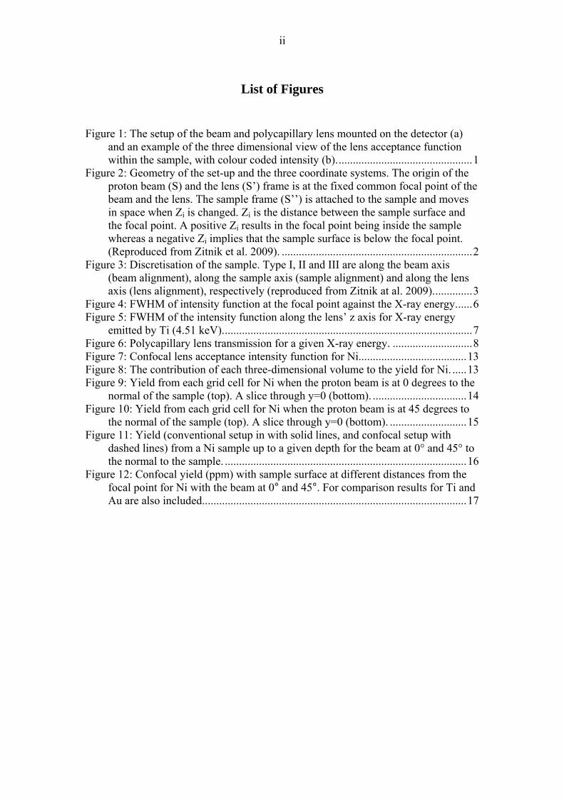
4.2. File configuration.txt The sample, detector and proton beam configuration is described to the program in the input file, configuration.txt, which has the following information. Line 1: 1 1 Line 2: 115.00000 0.00000 45.00000 6.00000 6.00000 1.000 Line 3: 2.60000 0.20000 3.00000

9

Line 4: 25.000000 0.000000 0.000000 0.300000 1.000000 0.000000 Line 5: 4 Line 6: 45.00 0.000 Line 7: 100 100 100 100 200 200 0.0 19300000 10 10 Line 8: AL SI P S CL K CA TI V CR MN FE CO NI CU ZN BR SR PBL END Line 9: AL SI P S CL K CA TI V CR MN FE CO NI CU ZN BR SR PB END Line 10: 1 1 1 1 1 1 1 1 1 1 1 1 1 1 1 1 1 1 1 Line 11: -30 30 10 Line 12: 1 Line 13: Title Line 14: trans = off Line 1: IPRT = 1 print intermediate results, =0 don’t print, IOUT = 1 print to the log file “conf_log.txt”, iout = 0 don’t generate log file Line 2: DIST THTIN THEOUT DIAM Poly_dist Poly_diam DIST – distance of the detector to the sample (mm) THTIN – angle between the beam and normal to the sample (clockwise) THEOUT – angle between the detector and normal to the sample (anticlockwise) DIAM – detector diameter (mm) Poly_dist – distance from polycarpellary lens to sample in mm Poly_diam – diameter of polycarpellary lens (mm) Line 3: EHI ELO CHARG proton energy EHI – incident proton energy MeV ELO – not used CHARG – charge in micro coulombs Line 4: XBE,XSI,XAU,XTHICK,FG,XICE – detector information Line 5: IFILT – filter type Line 6: THICK HOLE – filter information Line 7: XRANGE YRANGE NXCELLS NYCELLS THICKNESS LAYERS Zs DENSITY XBEAM YBEAM XRANGE – Beam x range micro meters = 2*XRANGE YRANGE – Beam y range micro meters = 2*YRANGE NXCELLS – number of cells in the x direction = 2*NXCELLS NYCELLS – number of cells in the y direction = 2*NYCELLS THICKNESS – sample thickness micro meters LAYERS – number of layers Zs – distance of sample surface from focal point, positive value implies that the focal point is Zs micro meters into the sample, whereas negative values implies that the focal point is outside of the sample

z

Positive z Focal point (0,0,0)

x Negative z

Sample With sample surface located at z = -10 micro meters, i.e. Zs is -10.

DENSITY – density of material grams / cm3

XBEAM beam in x direction micro meters YBEAN beam in y direction micro meters Line 8: list of elements, but need e.g. PBL for PB Line 9: list of matrix elements e.g. without the L for PB Line 10: concentration of each element Line 11: z1 z2 zinc Loop over the location of the surface of the sample in relation to the focal point. Start with location of sample surface at z1 microns from the focal point. Calculate the yield for this location, then

10

increment the location by zinc and repeat the calculation. Repeat the incrementing the location of the surface of the sample and recalculation of the yield until z2 is reached. Line 12: IGENPLOT – 1 generate a tecplot files 0 don’t generate the plot Line 13: Title to appear in tecplot file Line 14: trans = off results in Lens transmission probability to be set to 1 else the actual probability is used.

4.3. Data files The input files dset3, dset4 and dset5 are also used. These are as for PIXE (Clayton et al., 1981).

4.4. Output files The confocalPIXEyld program generates up to 3 output files:

• conf_log.txt which contains the yield information and contains the same information to what is printed on the screen

• XYZtaget.dat – a file that is optionally produced which contains the three dimensional data for plotting in tecplot.

• Zyield.dat – a file that is optionally produced and contains the yield when the location of the target surface is varied.

The contents of conf_log.txt are reproduced in Appendix 1.

5. Verification

5.1. Verification against PIXE The confocalPIXEyld program generates the yield for a thick target for a detector without the lens as well as the yield for the confocal setup, by performing the volume integration. The yield for the thick target has been compared against that obtained for conventional PIXE, for the same configuration, (Table 2) and it was found that for most elements the difference in yield was 1% or less.

Table 2: Yield (ppm) as generated by conventional PIXE and that of confocalPIXEyld (volume integrated).

PIXE Volume Integration

MG 1.09080 1.02660AL 6.68971 6.73884SI 21.38400 21.53830P 11.50900 11.58300S 19.06390 19.25000CL 25.75850 26.03700K 37.22700 37.55910CA 40.50400 40.81400TI 35.72800 35.95160V 32.04000 32.22300CR 29.07000 29.22400MN 24.59280 24.72200FE 21.02330 21.12900CO 16.99000 17.08300NI 14.30000 14.37400

11

CU 10.95170 11.01600ZN 8.67000 8.72300AS 3.57950 3.60440BR 1.86678 1.88050SR 0.65233 0.65750ZR 0.31326 0.31500MO 0.14909 0.15000RU 0.07077 0.07140AG 0.02384 0.02400SN 0.00798 0.00806

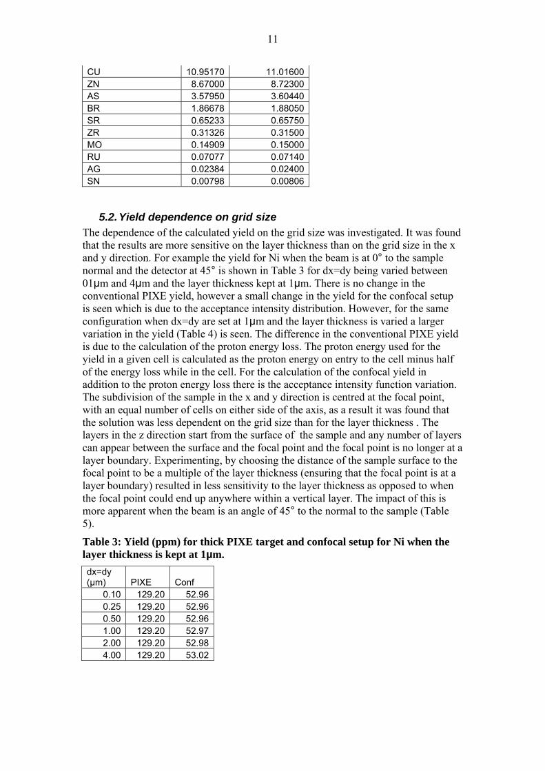
5.2. Yield dependence on grid size The dependence of the calculated yield on the grid size was investigated. It was found that the results are more sensitive on the layer thickness than on the grid size in the x and y direction. For example the yield for Ni when the beam is at 0° to the sample normal and the detector at 45° is shown in Table 3 for dx=dy being varied between 01µm and 4µm and the layer thickness kept at 1µm. There is no change in the conventional PIXE yield, however a small change in the yield for the confocal setup is seen which is due to the acceptance intensity distribution. However, for the same configuration when dx=dy are set at 1µm and the layer thickness is varied a larger variation in the yield (Table 4) is seen. The difference in the conventional PIXE yield is due to the calculation of the proton energy loss. The proton energy used for the yield in a given cell is calculated as the proton energy on entry to the cell minus half of the energy loss while in the cell. For the calculation of the confocal yield in addition to the proton energy loss there is the acceptance intensity function variation. The subdivision of the sample in the x and y direction is centred at the focal point, with an equal number of cells on either side of the axis, as a result it was found that the solution was less dependent on the grid size than for the layer thickness . The layers in the z direction start from the surface of the sample and any number of layers can appear between the surface and the focal point and the focal point is no longer at a layer boundary. Experimenting, by choosing the distance of the sample surface to the focal point to be a multiple of the layer thickness (ensuring that the focal point is at a layer boundary) resulted in less sensitivity to the layer thickness as opposed to when the focal point could end up anywhere within a vertical layer. The impact of this is more apparent when the beam is an angle of 45° to the normal to the sample (Table 5).

Table 3: Yield (ppm) for thick PIXE target and confocal setup for Ni when the layer thickness is kept at 1µm. dx=dy (µm) PIXE Conf

0.10 129.20 52.96 0.25 129.20 52.96 0.50 129.20 52.96 1.00 129.20 52.97 2.00 129.20 52.98 4.00 129.20 53.02

12

Table 4: Yield (ppm) for thick PIXE target and confocal setup for Ni when dx=dy are kept at 1µm and the layer thickness (dz) is varied. dz (µm) PIXE Conf

0.10 129.00 52.89 0.25 129.10 52.91 0.50 129.10 52.93 1.00 129.20 52.27 2.00 129.30 53.02 4.00 129.10 53.07

Table 5: Yield (ppm) for thick PIXE target and confocal setup for Ni when dx=dy=dz are varied. dx=dy=dz (µm) PIXE Conf

0.10 159.80 43.51 0.25 159.90 43.51 0.50 160.10 43.00 1.00 160.30 42.75 2.00 160.60 43.72 4.00 160.60 39.74

6. Example – Nickel (Ni)

6.1. Wide beam In order to illustrate the volume formed by the intersection of the beam and the confocal lens acceptance intensity function a beam of 80x80 μm was used on a Ni target. The angle of the proton beam to the normal to the sample surface was chosen as 0° and the detector placed at a 45° angle to the normal to the sample surface. The confocal lens acceptance intensity function is shown in Figure 7, where the highest intensity is seen along the lens’ z-axis (note the z-axis in the diagram is relative to the target, and the z-axis relative to the lens is at 45° to this axis). The contribution to the total yield from each three-dimensional volume is presented in Figure 8. The shape of the volume is as a result of a number of contributing factors:

• The depth penetration of the proton in the sample • The attenuation of the X-ray by the material • The confocal lens acceptance intensity function.

The larger yield (orange region in Figure 8) is produced when the beam intersects with regions of higher value of the confocal lens acceptance function (see Figure 7). On any xy-plane the largest yield is produced along the confocal lens’ z-axis and then we see a reduction in the yield as we move out of this region. In addition a reduction of the yield is seen as we move down the sample due to the reduced proton energy and then the larger attenuation of the X-rays travelling to the detector from further in the sample.

13

Figure 7: Confocal lens acceptance intensity function for Ni.

Figure 8: The contribution of each three-dimensional volume to the yield for Ni.

14

6.2. Narrow beam The set up is more likely to be used with a narrow beam to target specific region of the sample. To illustrate tis two configurations were compared for the simulation of a sample of pure Ni. In both configurations the detector is placed at a 45° angle to the normal to the sample surface. However, the angle of the proton beam to the normal to the sample surface was chosen as 0° for one simulation (Figure 9) and as 45° for the second simulation (Figure 10).

Figure 9: Yield from each grid cell for Ni when the proton beam is at 0 degrees to the normal of the sample (top). A slice through y=0 (bottom).

15

Figure 10: Yield from each grid cell for Ni when the proton beam is at 45 degrees to the normal of the sample (top). A slice through y=0 (bottom). The yield from the sample up to a given depth is presented in Figure 11. The conventional PIXI yield (solid lines) is larger when the beam is at 45° to the normal to the sample as the beam is at a smaller distance from the surface of the sample, thus the attenuation of the emitted X-rays is lower. However, for the confocal setup the yield at 45° is less than that at 0° degrees. This is due to the confocal spatial intensity function and the point at which the beam intersects. In addition to the angles at which the beam and detector are positioned the distance of the sample surface from the beam

16

and lens focal point play a role in the resulting yield (see Figure 12). Comparing the slice through the y=0 plane in Figures 9 and 10, we can see that a larger proportion of the beam intersects with higher intensity acceptance function when the beam angle is at 0°.

Sample depth (micro m)

Yie

ld(p

pm)

0 10 20 30 40 500

20

40

60

80

100

120

140

160

0 yld0 Conf. Yld45 Yld45 Conf. Yld

Ni

Figure 11: Yield (conventional setup in with solid lines, and confocal setup with dashed lines) from a Ni sample up to a given depth for the beam at 0° and 45° to the normal to the sample. Varying the location of the sample surface in the z-direction shows that the maximum yield for Ni is obtained when the sample surface is located at 6μm from the focal point (Figure 12, also includes results for Ti and Au). For comparison Ti and Au are also included in Figure 12. The emitted X-ray energy for Ti, Ni and Au are 4.51, 7.477 and 9.712 (keV) respectively. These X-ray energies correspond to a FWHM at the focal point of 47.48, 37.53 and 34.02 (μm) for Ti, Ni and Au, respectively. When the beam was at 45° to the normal to the sample surface the maximum yield was obtained when the sample surface was at 8, 6 and 2 (μm) from the focal point (for Ti, Ni and Au respectively) which is a result of the lens acceptance intensity function.

17

Sample surface distance from focal point

Yie

ld

-50 0 500

10

20

30

40

50

60

70Ti 0Ti 45Ni 0Ni 45Au 0Au 45

Figure 12: Confocal yield (ppm) with sample surface at different distances from the focal point for Ni with the beam at 0° and 45°. For comparison results for Ti and Au are also included.

7. References Andersen H.H, Ziegler J.F. 1977. The stopping and Range of Ions in Matter, Vol 3. Pergamon Press, New York. Clayton E., Cohen D.D., Duerden P. 1981. Thick target PIXE analysis and yield curve calculations. Nuclear Instruments and Methods 180, 541-548. Theisen R., Vollath D., 1967. Tables of X-ray Mass Attenuation Coefficients. Verlag Stahleisen, M.B.H. Dusseldorf. Wernisch J., Pohn C., Hanke W., Ebel H., 1984. μ/ρ Algorithm valid for 1keV ≤ E ≤ 50keV and 11 ≤ Z ≤ 83. X-Ray Spectrom, 13:180. Wolff T., Mantouvalon I., Malzer W., Nissen J., Berger D., Zizak I., et al., 2009. Performance of a polycapillary halflens as focussing and collecting optic – a comparison. Journal of Analytical Atomic Spectrometry, 24, 669-675. Zitnik M., Pelicon P., Bucar K., Grlj N., Katydas A.G., Sokaras D., Schutz R., KanngieBer B., 2099. Element-selective three-dimensional imaging of microparticles with a confocal micro-PIXE arrangement. X-Ray Spectrometry 38, 526-539.

8. Appendix 1: File conf_log.txt The contents of the output file conf_log.txt are form 4 main groups:

1. Reproduction of the input data configuration.txt

18

2. A list of parameters and their values to be used in the calculation 3. The yield for each layer of the sample 4. The yield as the position of the sample surface relative to the focal point is

varied. These are labelled in the following file contents. 1. Reproduction of the input file, configuration.txt The yield calculation data set is ******************************************************************************* * 42.00000 0.0000 45.00000 4.00000 6.00 0.94 * * 4.00000 0.10000 3.00000 * * 25.000000 0.100000 0.020000 4.230000 1.000000 0.000000 * * 1 filter 1 for mylar 2 pespex 3 kapton 4 graphi * * 0.1400 0.000 * * 40 40 80 40 160 160 18.8 8.902 13.2 8 xrnge,yrnge,nx,ny,zrnge,nzs,Zstart,de * * NI END Elt * * NI END Matrix + composition * * 1 0.000001 0.000001 0.000001 * * -30 30 5 Vary Zs by 5 starting at -30 to 30 * * 1 one to generate tecplot zero not to generate tecplot output * * 4 MeVp on Ni Q=3µC 140µm Mylar 10x10µm beam at 90 degrees * * trans = on IF off transmission is 1 otherwise use polynomial * *******************************************************************************

2. Parameter values used in the simulation Detector parameters Be window 25.000 Si deadlayer 0.100 Gold contact 0.020 Thickness 4.230 FG 1.000 Ice thickness 0.000 Filter type is 1 Thickness and hole fraction 0.140 0.000 4 MeVp on Ni Q=3µC 140µm Mylar 10x10µm beam at 90 degrees Accumulated Charge (microCoulombs) 3.00 Solid angle (Steradians) 7.124D-03 Conf. Solid angle (Steradians) 1.928D-02 Number of protons 1.872D+13 Detector diameter (mm) 4.00 Detector distance (mm) 42.00 Polycapillary distance (mm) 6.00 Polycapillary diameter (mm) 0.94 Incident proton Energy (MeV) 4.000D+00 Low proton Energy (MeV) 1.000D-01 Beam angle (deg) 0.00 Detector angle (deg) 45.00

19

Density (g/cm^3) 8.90 Theoretical gain 2.71 Beam dimensions (micro m) x 13.20 y 8.00 Dimensions (micro m) x 80.00 y 80.00 dx 0.50 dy 1.00 z 160.00 Zs 18.80 z modelled 160.00 dz modelled 1.00 ************* Yld, EXR NI 7.47700D+00 EFFICIENCY 0.8344 SIGMAX SIGMAI 1.579D+02 4.415D+02 Element, Xray energy, Lens transmission NI 7.48 0.18 NI X-Ray Energy 7.4770 WK 4.060D-01 ALPHAK 8.811D-01 A WEIGHT 58.7100 NI (conc, mu) 1.0000 59.1027 Total mu 59.1027 3. Yield as each layer of the sample is processed. For each layer the yield over the two dimensional region making up the layer is estimated. The total up and including that layer is then displayed. Layer Energy(MeV) Depth Rhox NI (micro m) (mg/cm2) Yld no poly Yld with poly 1 3.951333 1.00 8.902E-01 1.221E+01 4.202E+00 2 3.902262 2.00 1.780E+00 2.335E+01 8.172E+00 3 3.852776 3.00 2.671E+00 3.352E+01 1.191E+01 4 3.802863 4.00 3.561E+00 4.279E+01 1.543E+01 5 3.752511 5.00 4.451E+00 5.125E+01 1.873E+01 6 3.701705 6.00 5.341E+00 5.895E+01 2.181E+01 7 3.650434 7.00 6.231E+00 6.596E+01 2.469E+01 8 3.598682 8.00 7.122E+00 7.234E+01 2.737E+01 9 3.546433 9.00 8.012E+00 7.814E+01 2.986E+01 10 3.493673 10.00 8.902E+00 8.341E+01 3.216E+01 11 3.440383 11.00 9.792E+00 8.819E+01 3.429E+01 12 3.386547 12.00 1.068E+01 9.253E+01 3.624E+01 13 3.332144 13.00 1.157E+01 9.646E+01 3.804E+01 14 3.277155 14.00 1.246E+01 1.000E+02 3.968E+01 15 3.221558 15.00 1.335E+01 1.032E+02 4.118E+01 16 3.165330 16.00 1.424E+01 1.061E+02 4.255E+01 17 3.108448 17.00 1.513E+01 1.088E+02 4.379E+01 18 3.050884 18.00 1.602E+01 1.111E+02 4.491E+01 19 2.992612 19.00 1.691E+01 1.133E+02 4.592E+01 20 2.933601 20.00 1.780E+01 1.152E+02 4.682E+01 21 2.873819 21.00 1.869E+01 1.169E+02 4.764E+01 22 2.813233 22.00 1.958E+01 1.184E+02 4.836E+01 23 2.751804 23.00 2.047E+01 1.198E+02 4.900E+01 24 2.689493 24.00 2.136E+01 1.210E+02 4.957E+01 25 2.626256 25.00 2.225E+01 1.221E+02 5.008E+01 26 2.562046 26.00 2.315E+01 1.231E+02 5.052E+01

20

27 2.496812 27.00 2.404E+01 1.240E+02 5.090E+01 28 2.430496 28.00 2.493E+01 1.247E+02 5.124E+01 29 2.363037 29.00 2.582E+01 1.254E+02 5.153E+01 30 2.294366 30.00 2.671E+01 1.260E+02 5.178E+01 31 2.224409 31.00 2.760E+01 1.265E+02 5.200E+01 32 2.153080 32.00 2.849E+01 1.269E+02 5.218E+01 33 2.080287 33.00 2.938E+01 1.273E+02 5.233E+01 34 2.005924 34.00 3.027E+01 1.277E+02 5.246E+01 35 1.929872 35.00 3.116E+01 1.279E+02 5.257E+01 36 1.851996 36.00 3.205E+01 1.282E+02 5.266E+01 37 1.772141 37.00 3.294E+01 1.284E+02 5.273E+01 38 1.690130 38.00 3.383E+01 1.286E+02 5.279E+01 39 1.605755 39.00 3.472E+01 1.287E+02 5.284E+01 40 1.518770 40.00 3.561E+01 1.288E+02 5.287E+01 41 1.428886 41.00 3.650E+01 1.289E+02 5.290E+01 42 1.335752 42.00 3.739E+01 1.290E+02 5.292E+01 43 1.238937 43.00 3.828E+01 1.291E+02 5.294E+01 44 1.137906 44.00 3.917E+01 1.291E+02 5.295E+01 45 1.031971 45.00 4.006E+01 1.291E+02 5.296E+01 46 0.920231 46.00 4.095E+01 1.292E+02 5.297E+01 47 0.801118 47.00 4.184E+01 1.292E+02 5.297E+01 48 0.673772 48.00 4.273E+01 1.292E+02 5.297E+01 49 0.535829 49.00 4.362E+01 1.292E+02 5.297E+01 50 0.383289 50.00 4.451E+01 1.292E+02 5.297E+01 51 0.208127 51.00 4.540E+01 1.292E+02 5.297E+01 Smallest proton energy reached at layer 52 Distance travelled (micro m), target depth (micro m), proton enery (MeV) = 51.00000000000001 51.00000000000001 0.2081267474449019 4. Yield as the position of the sample surface relative to the focal point is changed. Total Yield from sum of volumes Sample Pos (z) NI (micro m) Yld no ploy Yld with pol 1.880E+01 1.292E+02 5.297E+01 ---------------------------------------------------------------------- -3.000E+01 1.292E+02 1.563E+01 -2.500E+01 1.292E+02 2.155E+01 -2.000E+01 1.292E+02 2.837E+01 -1.500E+01 1.292E+02 3.571E+01 -1.000E+01 1.292E+02 4.296E+01 -5.000E+00 1.292E+02 4.944E+01 0.000E+00 1.292E+02 5.443E+01 5.000E+00 1.292E+02 5.736E+01 1.000E+01 1.292E+02 5.787E+01 1.500E+01 1.292E+02 5.593E+01 2.000E+01 1.292E+02 5.181E+01 2.500E+01 1.292E+02 4.601E+01 3.000E+01 1.292E+02 3.921E+01 confocalPIXEyld completed

9. Appendix 2 – file configuration.txt for the simulation of Ni The contents of the configuration.txt file for the simulation of Ni is as follows: 1 1 42.00000 0.0000 45.00000 4.00000 6.00 0.94

21

4.00000 0.10000 3.00000 25.000000 0.100000 0.020000 4.230000 1.000000 0.000000 1 filter 1 for mylar 2 pespex 3 kapton 4 graphite 0.1400 0.000 40 40 80 40 160 160 18.0 8.902 13.2 NI END Elt NI END Matrix + composition 1 -30 30 5 Vary Zs by 5 starting at -30 to 30 1 one to generate tecplot zero not to generate tecplot output 4 MeVp on Ni Q=3µC trans = on