Joint Completion Report on IDNP Redt # 3 "Computer Modeling in Irrigation and Drainage" 7. DESIGN AND EVALUATION OF SURFACE IRRIGATION METHODS IN SOUTHERN GUJARAT USING SURDEV (GAU) 7.1 Introduction The study area is located in the central western coast of India in the Southern Gujarat. South Gujarat comprises of the Valsad, the Navsari, the Dang, the Surat and the Bharuch districts with rainfall varying from about 850 mm to 2000 mm. The general topography of the area is flat. The soils of the area are clayey while some parts also have clay loamsoils. The main crops of the South Gujarat are sugarcane, paddy and fruit crops. Paddy is taken both during khavifand summer seasons. Sugarcane crop occupies more than 50% of the culturable command area in South Gujarat and it is mostly irrigated with furrow method of irrigation. Furrow method of irrigation is also adopted for many other vegetable crops of this area. Paddy and fruit crops like banana, mango, and papaya are irrigated using basin irrigation method. In fruit crops, ring basin method of irrigation is adopted. In paddy, farmers adopt field to field irrigation. The area, in addition to heavy rainfall, receives canal water throughout the year. The region has many streams flowing from eastern side and draining into the Arabian Sea. Farmers of the region, due to easy availability of water, knowingly or unknowingly apply more water, especially in the upper reaches of the canal. On the other hand, in mid and tail reaches of canal command and in well-irrigated areas, the water application is less than the demand and is non-uniform. Drip irrigation method is common for fruit crops. However, high initial investments; non- availability of after-sales service; lack of technical knowhow; and poor designs of the system has discouraged the farmers from adopting the drip method of irrigation. The advantage of the drip irrigation method is also achievable with surface irrigation methods if the land is perfectly graded and systems are properly designed and managed. In order to achieve this, a computer model has been developed at ILRI and is named as SURDEV. The SURDEV model package consists of three different models: BASDEV for basin design, FURDEV for furrow design and BORDEV for border design. The three models can be used for the design) operation and evaluation of these methods. In the present study, on the basis of the data collected from the field, an attempt has been made to assess the design parameters of basin and furrow irrigation method so as to attain high on-farm irrigation efficiencies. 7.2 Model Parameters The variables involved in surface irrigation modelling are classified in two categories: field parameters and decision variables. Field parameters include the infiltration characteristics, the surface roughness or flow resistance and the required irrigation depth. In border and furrow irrigation, the gradient in the downstream direction is also a field parameter. In furrow irrigation, the shape and spacing of the furrows are also field parameters. 33
Transcript
Joint Completion Report on IDNP R e d t # 3 "Computer Modeling in Irrigation and Drainage"
7. DESIGN AND EVALUATION OF SURFACE IRRIGATION METHODS IN SOUTHERN GUJARAT USING SURDEV (GAU)
7.1 Introduction
The study area is located in the central western coast of India in the Southern Gujarat. South Gujarat comprises of the Valsad, the Navsari, the Dang, the Surat and the Bharuch districts with rainfall varying from about 850 mm to 2000 mm. The general topography of the area is flat. The soils of the area are clayey while some parts also have clay loamsoils. The main crops of the South Gujarat are sugarcane, paddy and fruit crops. Paddy is taken both during khavifand summer seasons.
Sugarcane crop occupies more than 50% of the culturable command area in South Gujarat and it is mostly irrigated with furrow method of irrigation. Furrow method of irrigation is also adopted for many other vegetable crops of this area. Paddy and fruit crops like banana, mango, and papaya are irrigated using basin irrigation method. In fruit crops, ring basin method of irrigation is adopted. In paddy, farmers adopt field to field irrigation.
The area, in addition to heavy rainfall, receives canal water throughout the year. The region has many streams flowing from eastern side and draining into the Arabian Sea. Farmers of the region, due to easy availability of water, knowingly or unknowingly apply more water, especially in the upper reaches of the canal. On the other hand, in mid and tail reaches of canal command and in well-irrigated areas, the water application is less than the demand and is non-uniform.
Drip irrigation method is common for fruit crops. However, high initial investments; non- availability of after-sales service; lack of technical knowhow; and poor designs of the system has discouraged the farmers from adopting the drip method of irrigation. The advantage of the drip irrigation method is also achievable with surface irrigation methods if the land is perfectly graded and systems are properly designed and managed. In order to achieve this, a computer model has been developed at ILRI and is named as SURDEV.
The SURDEV model package consists of three different models: BASDEV for basin design, FURDEV for furrow design and BORDEV for border design. The three models can be used for the design) operation and evaluation of these methods. In the present study, on the basis of the data collected from the field, an attempt has been made to assess the design parameters of basin and furrow irrigation method so as to attain high on-farm irrigation efficiencies.
7.2 Model Parameters
The variables involved in surface irrigation modelling are classified in two categories: field parameters and decision variables. Field parameters include the infiltration characteristics, the surface roughness or flow resistance and the required irrigation depth. In border and furrow irrigation, the gradient in the downstream direction is also a field parameter. In furrow irrigation, the shape and spacing of the furrows are also field parameters.
33
Joint Completion Report on IDNP Result ## 3 "Computer Modeling in lrrigation and Drainage"
In the present study, SCS intake families are used to describe the infiltration characteristics of the soil. SCS intake families # 0.1 and 0.3 can be used to represent clay soils and SCS intake families 0.3 and 0.5 for clay loam soils (Table 19). This table also shows the corresponding values of the infiltration constant and infiltration exponent of the Kostiakov equation. In various model runs, the flow resistance was taken as 0.15 and it was assumed that 80 mm depth of water is needed per irrigation.
Decision variables are those parameters or variables that a design engineer can manipulate to obtain the best irrigation performance for given or selected field parameters. The decision variables in surface irrigation are normally the field size (length and width), the discharge and the cut-off time. In various runs, commonly used field sizes and discharges were used.
Table 19. Model infiltration characteristics
Soil class' SCS family Parameters of Kostiakov equation
K (mm I minA) A (4 Clay, silty clay 0.1 1.10 0.595
Silty clay, clay loam Clay loam, loam
0.3 0.5
1.59
1.93
0.650
0.684
7.3 Application of BASDEV for Basin Design
The data collected at Segwa pilot area were used as input for designing the optimum time of irrigation. From field observations it was observed that most paddy fields vary from 10 m x 10 m, 20 m x 20 m, 30 m x 20 m, 40 m x 30 m. Some additional dimensions of the basins are also included. The water discharge from different wells ranged from 10 to 15 Ips. An attempt was also made to measure the discharge from the canal, but since canal discharge enters at several points in the farmers' field, especially at the head reaches of the canal, it was difficult to measure. However the discharges in the mid and tail reaches of the canal are comparable with the well discharges. Two additional discharges of 20 and 25 Ips have also bken considered.
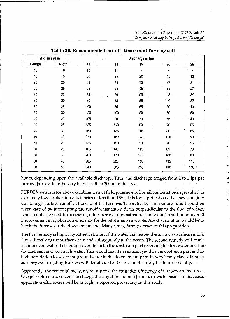
For each combination of field size and available discharge, the BASDEV model was run in such a way that high application, storage and distribution efficiencies were achieved by optimising the cut-off time of irrigation. Table 20 shows the recommended cut-off times for current discharges; these are applicable both for clay soils as well as for clay loam soils.
The above recommended cut-off times will result in application efficiencies of at least 80% and under-irrigation at the downstream end of the basins would not be more than 10% of the application depth.
7.4 Application of FURDEV for Furrow Evaluation
The FURDEV model was applied to evaluate the existing practices of farmers irrigating sugarcane in the Segwa pilot area. It was observed that at a time, farmers open 3 to 5 furrows for 8 to 10
34
Joint Completion Report on IDNP Result # 3 “Computer Modeling in Irrigation aizd Drainage”
Table 20. Recommended cut-off time (min) for clay soil
Field size in m Discharge in Ips Length Width 10 12 15 20 25
10 10 13 15 15 30
20 20 55
20
25
30
30
30 40
40
40 40
50 50
50 50 50
25
25
20
25
30
20 25
30
40
20
25
30
40
50
65
85
80
1 O0
120
105 135
160
210
135
165
200
285
340
11
25 20 15 12
45 35 27 21
55 70
65
85
1 O0
90
110
135
180
120
140
170 225
300
45
55
55 65
80
70
90
105
140
90
120
140 180
250
35
42
40
50 60 55
70
80
110
70
85
1 O0
135 180
27
34
32
40
50 * 43
55 65
90
55
70
80 110
135
t
...
I
. . I
.t
c i
hours, depending upon the available discharge. Thus, the discharge ranged from 2 to 3 Ips per 1
furrow. Furrow lengths vary between 30 to 100 m in the area.
FURDEV was run for above combinations of field parameters. For all combinations, it resulted in
due to high surface runoff at the end of the furrows. Theoretically, this surface runoff could be taken care of by intercepting the runoff water into a drain perpendicular to the flow of water, which could be used for irrigating other furrows downstream. This would result in an overall improvement in application efficiency for the pilot area as a whole. Another solution would be to block the furrows at the downstream end. Many times, farmers practice this proposition.
!
J
extremely low application efficiencies of less than 15%. This low application efficiency is mainly 7,
The first remedy is highly hypothetical; most of the water that leaves the furrow as surface runoff, flows directly to the surface drain and subsequently to the ocean. The second remedy will result in an uneven water distribution over the field; the upstream part receiving too less water and the downstream end too much water. This would result in reduced yield in the upstream part and in high percolation losses to the groundwater in the downstream part. In very heavy clay soils such as in Segwa, irrigating furrows with length up to 100 m cannot simply be done efficiently.
Apparently, the remedial measures to improve the irrigation efficiency of furrows are required. One possible solution seems to change the irrigation method from furrows to basins. In that case, . application efficiencies will be as high as reported previously in this study.
35
Joint Completion Report on IDNP Result # 3 "Computer Modeling in lrrigation and Drainage"
7.5 Conclusions and Recommendations
On the basis of applications of the BASDEV and FURDEV models in this study, the following conclusions and recommendations are formulated:
The SURDEV model is an effective tool for developing guidelines to optimise the irrigation performance in level basin irrigation and for judging the irrigation performance in existing furrow irrigation.
The prepared tables for level basin irrigation can be readily used as a guideline in Southern Gujarat for maximising the irrigation efficiencies for specific field sizes and available discharges. Similar guidelines could be prepared for other surface irrigation methods or for other areas.
Under the prevailing conditions, furrow irrigation in heavy clay soils should be applied with care. Experiments should be framed where furrow irrigation is replaced by basin irrigation in farmers' fields to assess the performance and crop yield.
. ".
Joint Completion Report on IDNP Result # 3 “Computer Modeling in lrrigation and Drainage”
8. SALT AND WATER BALANCE MODELING: THE SEGWA PILOT AREA (GAU)
8.1 Introduction
Ukai-Kakrapar is a major irrigation project in South Gujarat. This is the biggest multi-purpose project built on the river Tapi. The Kakrapar weir was constructed as stage I and regular irrigation in its command commenced in 1957. The Ukai dam was constructed as stage I1 and regular irrigation and construction of Ukai canal distributary system was started in 1974 and completed by 1983. The total cultivable command area of the project is 3.31 lakh ha distributed in Surat (1.9 lakh ha), Valsad (0.96 lakh ha) and Bharuch (0.45 lahk ha) districts.
,
I
Before inception of the canal irrigation, farmers used to take only one rain fed crop during kharif
also grown in a small area. The groundwater table was at around 10 m depth. So most of the good quality rainwater percolated into the soil. There were only few open wells and ponds in every village, which were used for domestic and drinking purposes. These water bodies eventually helped to recharge the deep aquifers. Due to thick vegetative cover all around and sustained ecosystem, rainwater leached all the accumulated salts during the year. Water table was deep and there was absolutely no salinity during that period.
With the inception of canal irrigation in mid seventies, cropping pattern changed significantly, the farmers switched to high water requiring and perennial cash crops. Due to shift in cropping pattern in the canal command areas, sugar factories came up which prompted farmers of adjoining areas also to shift to sugarcane and paddy cultivation. The other important crops of the command which were formerly grown in the rainy season are now cultivated in the rabi / summer season under irrigated conditions. With the availability of cheap irrigation water, many head end farmers use excessive amounts of water. The excessive use of irrigation water combined with high rainfall in the area led to a rapid rise of the water table, resulting in the development of waterlogging and salinity in large areas. The use of poor quality irrigation water in non-command areas introduced another dimension to the problem of soil salinization in the command. The water table in Ukai Kakrapar command rose ralatively faster than other commands. The area where water table is within 1.5 m and 1.5 to 3.0 m cover an area of 13,000 ha and 1,06,000 ha respectively. Though no regular survey data on salt-affected soils is available, it is estimated that about 60,000 ha of the command area has problem of salinity, particularly in the coastal areas.
Models are effective tools for studying the effects of certain interventions if they are implemented in the field. In pilot area research, only a limited number of field experiments can be framed whereas many more combinations of parameters are actually possible. Therefore, it is very useful to calibrate a model on the basis of pilot area studies and use it for studying various scenarios. Data collected from the pilot area during the last six years of the project have been used to develop various scenarios of salt build-up and status of the water table using SALTMOD.
season. The main crops at that time were pigeon pea, sorghum, etc. However, kharifpaddy was ‘i
- 1
37
Joint Completion Report on IDNP Result # 3 “Conzputer Modeling in Irrigation and Drainage”
8.2 Study Site
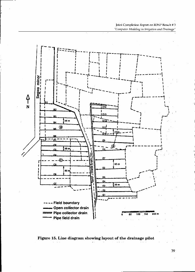
A 188 ha block (Fig. 15) in Segwa minor of Surat branch in Kakrapar irrigation command was selected for operational research on drainage and related water management. It is located in between 73” 2’ 51” to 73” 3‘ 25” E longitudes and 21” 12’ 18” to 21” 13’ 31” N latitudes. The site encompasses four villages namely Segwa, Sevni, Asta and Vansda Rundhi in the Kamrej taluka of the Surat district at the Segwa minor ex. Surat branch of Kakrapar Left Bank Main Canal. The area is bounded in the North by Surat branch, Natural drain in South, Segwa minor in the west and a cart road in the East. This area is about 10 km inside towards East of Bombay-Ahmedabad road (National highway No. 8). A metalled road-joining village Segwa and Vansda Rundhi is bifurcating the area towards the East and the West. About one third of the area on the eastern side of this road is irrigated by tube wells while remaining is irrigated through canal water. Conjunctive use of water is also made in some parts of the canal command. Waterlogging coupled with initiation of secondary salinisation is deteriorating the soil health and crop productivity in the pilot area.
8.3 Model Calibration and Validation
The data used in SALTMOD are collected before and after the installation of drainage system. The model was calibrated by using the data on cropping pattern, water table, hydraulic conductivity, salinity status, leaching efficiencies, drain discharges etc. Tbe input parameters used in calibrating the model are shown in Tables 21 and 22.
Table 21. Season-wise input parameter for use in SALTMQD
S.No.Parameters Season 1 Season 2 Season 3
1
2
3
4
5
6
7
8
9
10
11
12
‘13
Duration 15Ih Jun to 1 5Ih Nov (5 months)
Crops grown Sugarcane, Paddy
Water sources Canal, Well
Fraction of area occupied by irrigated crop other than rice 0.60
Fraction of area occupied by irrigated rice crop 0.15
Fallow /barren 0.25
Rainfall (m) 0.90
Water used for irrigation in crops other than rice (m)
Water used for irrigation in rice crop (m)
Potential evapotranspiration of crops other than rice (m)
0.30
0.65
0.80
1.35
0.80
Potential evapotranspiration of rice crop (m)
Potential evapotranspiration from unirrigated area (m)
Outgoing surface runoff (m) 0.28.
16Ih Nov to 15th Mar (4 months)
Sugarcane
Canal, Well, Drain
0.75
0.00
0.25
0.02
1 .o0
0.00
0.50
0.00
0.70
16th Mar to 1 5Ih Jun (3 months)
Sugarcane, Paddy
Canal, Well, Drain
0.60
0.15
0.25
0.10
0.80
1.40
0.50
0.90
0.75 I ,
Joint Completion Report on IDNP Result # 3 "Computer Modeling in lrriga tion and Drainage"
f\ N
! r-' Í t 1
f
t
- \ II
I 4 k - - - ~ r - i - - - - - - - - - J
4 EP .*A .
*cc -
-- -. Field boundary - Open collector drain = Pipe collector drain - Pipe field drain
0-150900 m
'i
Figure 15. Line diagram showing layout of the drainage pilot . *
39
Joint Completion Report on IDNP Result # 3 "Computer Modeling in Irrigation and Drainage"
Table 22. Other input parameter for use in SALTMOD I S.No Parameter Value
1 2 3 4 5 6 7 8 9 10 11
12 13 14
Storage efficiency Depth of root zone Depth of transition zone Depth of aquifer Total pore space of root zone Total pore space of transition zone Total pore space of aquifer Effective porosity of root zone Effective porosity of transition zone Effective porosity of the aquifer Initial salt content of the soil moisture (dS/m) at field saturation in
-Root zone -Transition zone -Aquifer
Mean salt concentration of irrigation water in the pilot area (dS/m) Initial depth of water table from ground surface Critical depth of water table for capillary rise
0.'75 0.85 6.0 50
0.50 0.50 0.60 0.05 0.05 0.20
12.0 7.0
0.9 1 .o 1.6
8.3.1 Determining the Natural Subsurface Drainage
Natural subsurface drainage (Gn = Go - GI) is defined as excess of the horizontally outgoing water minus the horizontally incoming groundwater in m / season. The values were determined by keeping value of G, as zero and arbitrarily changing the Go values to find values of depth to water table (Dw) and Gd that correspond with the observed values. The annual Go values of O, . O M , .020, .040, .050, .075,0.100 and 0.125 were considered. Table 23 shows final Dw and Gd values after one year of installation of the drainage system. This table shows that observed values coincided with Gn values at around 0.018.
Table 23. Determination of natural drainage
Season 1 Season 2 Season 3 Gn Gd Dw Gd Dw Gd Dw .o00 .O1 8 .O20 .O40 .O50 .O75 .loo ,125
Joint Completion Report on IDNP Result # 3 "Computer Modeling in lrngation and Drainage"
8.3.2 Calibration of Leaching Efficiency
Leaching efficiency of the root zone (Flr) is given arbitrary values of 0.2, 0.4, 0.6, 0.8 and 1.0 and the corresponding salinity results are compared with the actual field observations. The graphical representations of leaching efficiencies of root zone and transition zone are depicted in Fig. 16 and Fig. 17 respectively. The observed salinities were found to be close when the Flr and Flx were given a value of 0.7. However, while calibrating the leaching efficiency of transition zone, very slight difference was observed amongst different efficiencies (Flx) mainly because of the existing subsurface drains, as they drain out the salts in the upper layer itself and only part of leached water passes through the transition layer. Further, after first three years irrespective of variation in the leaching efficiency of transition zone, the root zone salinity is not affected.
-+- Flr = 0.2 + Flr = 0.4 -&- Flr = 0.6 * Flr = 0.7 ili Flr = 0.8 + F l r = 1 +observed
Figure 16. Calibration of the leaching efficiency of the root zone
l4 W l
O ' O I 2 2 3 4 4 5 6 6 7 8 8 9 1 0 1 0
Time after installation of drain (vrs)
&FIX = 0.2
-w- FIX = 0.4
-+- FIX = 0.6
+FIX = 0.7
+ FIX = 0.8
+FIX = 1.0
+ Observed
Figure 17. Calibration of the leaching efficiency of the transition zone
Joint Completion Report on IDNPResult ## 3 "Computer Modeling in lrrigation and Drainage"
8.4 Scenario Building
8.4.1 Prediction of Soil Salinity with Drainage System
Predicted of salinities for 10 years period after installation of subsurface drainage system are shown in Fig. 18. The root zone salinity (Cr4) decreased form 12 dS/m to around 7 dS/m in the first year and after 3 years the salts get leached to the acceptable limit of 2 to 3 dS/m. The soil salinity above drain level (Cxa) increased from 7 dS/m to around 9 dS/m during the first year, as salts leached from the top layers built-up the salinity above drain level. Thereafter, the Cxa values constantly declined reaching the acceptable range in third year and varying from 2 to 3 dS/m thereafter. However, the soil salinity below drain level (Cxb) declines at slower pace and would come below 4 dS/m only after 10 years. The figure shows an interesting feature that the salinity of the aquifer zone (Cqf) which was assumed to be 2 dS/ m shows slight increase with time because part of the leached salts from the upper layers would percolate to the aquifer zone.
O 0 1 2 2 3 4 4 5 6 6 7 8 8 9 1 0 1 0 Time after installation of drains (yrs) i OL---
Figure 18. Behaviour of salinity of the root, transition, aquifer zones following drainage
,
8.4.2 Reconstruction of the Initial Situation
Prediction of salinities for 10 years period without subsurface drainage system is shown in 1
Fig. 19. The model calculates the ayerage soil salinity of the whole pilot area in the rooting zone. It varies from 6 to 7.dS/m and shows a steady increase, though at a slow pace over the years, reaching the levels of 8 dS/m in second season of loth year. This figure also depicts that after first year during kharifseason, Cr4 values are the lowest in the rooting zone because good quality rainwater leaches down the salts from the top layer. During rabi and summer seasons due to capillary action the salts accumulation is more than kharif season. The model predicts that salt concentration of transition zone increases from 2.5 dS/m to 3.5 dS/m in 10 years. The salt concentration in the aquifer remains at 2 dS/m level.
42
Joint Completion Report on IDNP Result ## 3 "Computer Modeling zn Irrigation and Drainage"
i
i I I
~ __ - - __-- I ~ i It- ' O
I
1 1 2 3 3 4 5 5 6 7 7 8 9 9 10
T i m e after installation of drains (yrs)
Figure 19. Simulated salinity in the root, transition and aquifer zones assuming no drainage in the pilot
8.4.3 Effect of Varying Drain Spacing on Root Zone Salinity
Variation in root zone salinities (Cr4) due to change in drain spacing, which would ultimately affect the QH1 relationship is depicted in Fig. 20. Therefore, with reference to the actual QH1 value of 0.0015, simulations were made using QH1 values which are lower by 20%, 40% and 60% of the actual value. The lesser than the present lateral drain spacing was not tested. It could be seen that only when the QH1 was 0.0006 (60 % less than .0015) the root zone salinity remained above 3 dS/m whereas in rest of the cases the salinities dropped and stabilised at around 2.5 dS/ m. It does indicate some possibility of increasing drain spacing from the present one. This observation needs field testing as by increasing the lateral drain spacing, cost of subsurface drainage could be reduced.
Figure 20. Root zone salinity at the end of rabi season as influenced by drain spacing
43
Joint Completion Report on IDNP Result # 3 “Computer Modeling in Irrigation and Drainage”
-
8.4.4 Effect of Varying Drain Depth and Irrigation Water Applied on Water Table
Depth of the water table due to variation in drain depths (Dd) and irrigation water supplies (IWS) is shown in Fig. 21. The model runs show that the water table remains 1 m below the ground level when the irrigation water supplies are kept at the same level or below the present supplies. Simdarly, the water table could be kept a t lower than 0.8 m below ground level only when the drain depth is either at the present level or more than the present level.
4
3.5
Change in parameter ! + D d , I -A- IWS
Figure 21. Depth to water table as influenced by changes in diffrent parameters
8.5 Conclusions and Recommendations
The model SALTMOD for the Segwa minor canal command, once it was calibrated and validated with the data collected in the Segwa pilot area, predicted fairly correct trends for both the water table and soil salinity.
Canal command areas are likely to get salinised if appropriate drainage intervention is not introduced.
SALTMOD is an effective tool to forecast water table and soil salinity under various situations and therefore, could help in the design of drainage systems once the basic input parameters are known.