Design & Construction of subsonic wind Tunnel focusing on...

Design & Construction of subsonic wind Tunnel

focusing on two dimensional contraction cone

profile using sixth order polynomial (Design of Subsnic Wind Tunnel Contraction cone profile through CFD Simulation)

Kashif Javed1

1Assistant Professor, Department of Mechanical,

Mechatronics & Manufacturing Engineering

University of Engineering & Technology, KSK Campus

Lahore, Pakistan

[email protected]

[email protected]

[email protected]

Mazhar Ali2

2Lecturer, Department of Mechanical Engineering,

University of Lahore, Pakistan

Student, Skolkovo institute of Science & Technology

(MIT collaboration), Moscow, Russia

[email protected]

[email protected]

Abstract

This research work is focused on design and construction of

subsonic laboratory wind tunnel with “Ma=0.1”.During wind

tunnel design, mostly difficulties arise in generating a profile

for contraction cone; that must be selected to achieve uniform

flow with negligible losses and boundary layer growth. Since,

the design of contraction cone requires proper selection of

polynomial equation, A sixth order polynomial was chosen to

get a smooth design of contraction cone. The design work was

completed through CFD analysis using “ANSYS-FLOTRAN”

in which velocity & pressure contour profiles were finalized

after analyzing 12 different contraction cone profiles. The

current research not only includes verification of contraction

cone design by comparing the velocity of air at different

sections obtained during CFD analysis with the experimental

values at corresponding points; but also covers proper

selection of low cost material for test section, diffuser,

contraction cone, instrumentation as well as size and type of

fan.

Keywords: 2D, contraction cone, design optimization, CFD,

subsonic, wind tunnel, manometer

Nomenclature:

Ρw Density of water (kg/mᶟ)

Ρa Density of air (kg/mᶟ)

g Gravitational acceleration (m/sec²)

hm Head of water in manometer (m)

P Pressure (Pa)

Pa Pascal (S.I Unit of Pressure)

a,b,c,d,e,f,g, Polynomial coefficients

Q Discharge (mᶟ/sec or ftᶟ/min)

h Height (m)

I Axial distance to point of inflection (m)

L Total length of contraction cone (m)

x, y Cartesian coordinates (streamwise, vertical)

α Curvature at inlet (/m)

‘ d/dx

‘’ d²/dx²

2D Two Dimensional

CFM Cubic Feet Per Minute

U Axial velocity (m/sec)

V Redial velocity (m/sec)

Y Redial distance (m)

X Axial distance (m)

A Area (m²)

1. INTRODUCTION

Wind tunnels have proven to be the most advantageous and demanding equipment in science and technology. They have been extensively used to understand the effects of air resistance on automotive and aeronautical objects. This research uses computational as well as experimental techniques in order to validate primarily the contraction cone design for a subsonic (low speed), open circuit, laboratory wind tunnel. The stated equipment was designed and fabricated for the purpose of carrying out research including testing and experimentation in laboratory on different Airfoils associated with small aerodynamic and automotive models. The maximum velocity attained at test section was 35 m/sec. Though the current work

Scientific Cooperations International Workshops on Engineering Branches 8-9 August 2014, Koc University, ISTANBUL/TURKEY

287

mailto:[email protected]





covers detailed analysis on all the parts of wind tunnel including diffuser, test section, fan & instrumentation; however attention has been focused on contraction cone designing (2D) in major using CFD modeling which was subsequently authenticated through experimentation after its construction. The 2D design of contraction cone was carried out using 6th degree polynomial wall profile with a square working section.

2. Literature Review

Wind tunnel is an essential tool in engineering, both for model

tests and basic research. Based upon the practical utilization of

this tool, a lot of work has been done in its designing. [1] The

definition of a wind tunnel as given by Pankhurst and Holder

(1952), is, “A device for producing a moving airstream for

experimental purposes”. [2] The first real scientific

investigation started into the fledgling field of aeronautics,

scientists hoping to achieve heavier than air flight soon realized

that they would need to understand airflow dynamics about an

airfoil in order to design a practical wing. Until the early 1700s,

natural wind sources such as high ridges and the mouths of

caves were used for early testing, so-called whirling arm

apparatus. Benjamin Robins is credited as being the first to use

a whirling arm for aeronautical study. Dissatisfaction with the

whirling arms led Frank H. Wenham to design and built a

twelve foot long blower tunnel with a steam powered fan. Sir

Hiram Maxim also put his efforts to construct a wind tunnel

with a three-foot diameter and twice the size of Wenham’s. [3]

The Wright brothers also made extensive use of a wind tunnel

during the development of their third flyer after their first two

failed to meet their expectations and so built their own six foot

wind tunnel. Since the 1930s, when the strong effect of free

stream turbulence on the shear layers became apparent,

emphasis has been laid on wind tunnels with low levels of

turbulence and unsteadiness. [4] A generalization of the Tsien

method of contraction-cone design was described in 1972 by

Raymond L. Barger and John T. Bowen. The design velocity

distribution was expressed in such a form that the required

high-order derivatives can be obtained by recursion. This

method was applicable to the design of diffusers and

converging-diverging ducts as well as contraction cones.[5]

Since the 1930s, when the strong effect of free stream

turbulence on the shear layers became apparent, emphasis has

been laid on wind tunnels with low levels of turbulence and

unsteadiness. Consequently most of high performance wind

tunnels were designed as closed type to ensure a controlled

return flow. It is possible with care to achieve high

performance from an open wind tunnel, thus saving space and

construction cost. A research on the whole design of the low

speed subsonic wind tunnel was conducted by R.D. Mehta and

P. Bradshaw. That not only covers design information but they

also covers selection information about the essential parts of

the wind tunnel. [6] In 1980’s researchers and scientist began

to develop more accurate designs for the development of 2D

and 3D- contraction cones for low speed wind tunnels. An

adaptive design procedure was introduced by James H. Bell

and Rabindra D. Mehta .This method proceeded by computing

the potential flow field and pressure distributions along the

walls of a contraction of given size and shape using a three-

dimensional numerical panel method. [7] In 1986 Jonathan H.

Watmuff described the analytical methods of contraction cone

design for subsonic wind tunnels. [8] For design of Laboratory

wind tunnels that commonly have velocity less than 50m/s,

Daniel Brassard introduced a special five degree polynomial

equation for the design of contraction cone profile followed by

the condition that wall profile was having zero first and second

order derivatives, further, inlet and outlet profile radii roughly

proportional to the area. The result was hoped to be the most

favorable combination of flow uniformity, thin boundary

layers, and negligible losses. [9] J.E. Sargison, G.J. Walker and

R. Rossi published his research which describes the design of a

2D contraction cone with 6th degree polynomial wall profile

for a wind tunnel with a square test section. The objective was

to design low speed subsonic wind tunnel with uniformity of

flow in the working section through CFD modeling with the

variation of inflection point and inlet curvature. [10, 11, 12, 3]

For designing low speed subsonic wind tunnel contraction with

Ma<0.3 using a 6th degree polynomial equation,

incompressible and adiabatic flow conditions can be

considered.

3. Current Reserch

3.1 Design Features:

This section covers discussion and selection of all the features of wind tunnel on the basis of which the contraction cone was designed.

3.1.1. Test Section:

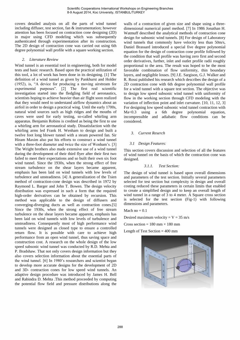
The design of wind tunnel is based upon overall dimensions and parameters of the test section. Initially several parameters selected for test section but complexity in design and overall costing reduced these parameters in certain limits that enabled to create a simplified design and to keep an overall length of wind tunnel in a range of 3 to 4 meter. A Square cross section is selected for the test section (Fig-1) with following dimensions and parameters.

Mach no = 0.1

Desired maximum velocity = V = 35 m/s

Cross section = 180 mm × 180 mm

Length of Test Section = 400 mm


288

Fig.1. 3D-Model of Test Section

3.1.2. Fan Selection

In order to select a proper size of fan, very simple procedure

was followed. Since the area of test section selected was “180

mm x 180 mm” or “0.36 sq. ft” and the velocity of air was “35

m/sec” or “117 ft/sec” so firstly, the volume flow rate of air at

test section was determined by the following equation.

Q = v x A

= 117 (ft/sec) x 0.36 (sq. ft)

= 42.12 cubic ft/sec = 2527.2 CFM

[3, 10, 11, 12] The above equation was used after assuming

the incompressible flow of air in test section due to low “Mach

number” (i.e. Ma < 0.3) [3, 10, 11, & 12]. The size of Fan was

based on desired CFM output. A fan was chosen with “15

inches” diameter and 1.5 hp motor which could move 3500

cubic feet of air per minute. This value was greater than the

desired CFM output i.e. 2527.2 CFM. The fan was in circular

metal frame with a flange of heavy gauge sheet metal at the

exhaust side. The frame houses a direct drive motor assembly

attached to fan hub and secured with a set screw. The fan itself

had seven cambered blades, also made from sheet metal, and

the whole unit was rated for an output of 3500 CFM with

variable output and following specifications in general.

Fig.2. Fan

A control box with a pull chain control drives the fan motor between the off position and a low and high speed setting. This limited the range of possible experimental velocities, so the power cable was connected to a variable output AC power supply with a maximum output of 440 volts. This Variable AC power supply allowed a much wider operating range, though performance suffered somewhat at extreme low or high velocities which were not taken during the analysis. A quick, back-of-the-envelope calculation predicted top centerline velocities in the neighborhood of about 35 m/s, or close to this value. Of course, this calculation was incredibly optimistic as the power losses due to honeycomb, screens, and contraction were completely neglected.

3.1.3. Diffuser:

Diffuser is an essential component of wind tunnel. It served dual functions in this project, besides of reducing the exhaust speed and hence reducing cost, it also served as a square to circular transition piece connecting the test section exit with the drive section. [5, 6] It has been determined that the flow through diffuser depends upon its geometry defined by area

ratio, and diffuser angle, wall contour and diffuser cross-sectional shapes. Other parameters like initial conditions, boundary layer control methods and presence of separation could also affect the flow thus making it very difficult to predict. Almost all the knowledge acquires about the diffuser is empirical [5, 6]. The length of diffuser section was calculated by size of fan, which was selected to be 15” in diameter. A square piece was designed and square portion turned out to be 450 x 450 mm. This became the dimensions of the end of the diffuser section. The diffusion angle was kept 6 degrees and ended up being 3 degrees on each side. This calculation made the diffuser section 1.5 m long (Fig-3).

Fig.3. 3D-Model of Diffuser

3.1.4. Contraction Cone:

The design of subsonic wind tunnel is mainly concerned with a 2-D design of Contraction cone. It was carried out using ANSYS FLOTRAN focusing on variation of two parameters [4, 6] i.e. inflection point (X/L) and Cone length (L) while areas and contraction ratio were kept constant. [9] Sixth order polynomial equation was used in order to optimize the contraction cone profile for acquiring laminar flow at the test section inlet [9]. Equation is given below

y = ax^6 + bx^5 + cx^4 + dx^3 + ex^2 + fx + g……(A)

The location of inflection point and lengths were varied for contraction cone for design optimization through CFD Analysis. The optimization was based on attaining the following results

Flow uniformity at the test section mid –plane

Prevention of separation in the contraction cone

Minimizing the boundary layer thickness at entrance to the test section.[5]

The contraction ratio was selected as 7 (6 to 9 are normally used), for low speed wind tunnels as recommended by Mehta [5]. The parameters that were kept unchanged are contraction ratio (i.e. 7), inlet area (i.e. 477 ×477 mm^2) and exit area (i.e.180×180 mm^2) of the contraction cone. The coordinate system for the contraction profile is defined by the origin present at the centre line of tunnel at inlet plane. Further, x-coordinate increases downstream and y coordinate defines the


289

contraction profile and z is in the span-wise direction

Fig 4: 3D-Model of Contraction cone

4. Mathematical Model

Equation (A) has 7 constants (a, b, c, d, e, f, g). Five of these are specified by the height at inlet and outlet, zero slopes at inlet and outlet as well as zero curvature at outlet. This leaves two parameters available for optimization. [9] These are specified by the inlet curvature (α) and the axial position of the point of inflection relative to the contraction length [9]. The “7” conditions defining the cone profile are given as.

(1) Y(x=0) =h , (2) Y’(x=0) =0, (3) Y’’(x=0)= α=0

(4) Y’’(x=i) =0, (5) Y(x=l) =0, (6) Y’’(x=l) =0,

(7)Y’(x=l) =0

Where h = inlet half height – exit half height.

Fig 5: Graphical representation of seven Boundary Conditions & Inflection Point.

An inflection point is a point on a curve at which the sign of the curvature (i.e., the concavity) changes. Inflection points may be stationary points, but are not local maxima or local minima. By using above boundary conditions, following mathematical models for contraction cone profiles were developed based upon different inflection points (i.e.i=0.4,0.5,0.6) and different lengths of contraction “l” (i.e. l -500, 750, 1000, 1250 mm).

4.1. Simulation

[9] It has been observed that more precise results (uniform

velocity) are obtained, if inflection point is selected

downstream the contraction cone as near as possible to the test

section [9]. Large contraction ratios and short contraction

lengths are generally more desirable as they reduce the power

loss across the screens and the thickness of boundary layers.

Further, for economical design, we need smaller length of

contraction cone for the required velocity (i.e. 35 m/sec) due

to lesser material and manufacturing cost. The proper selection of contraction cone profile for wind tunnel was decided on the basis of computer based modeling and simulation tools. In this method, after deriving equations

1- For inflection point (i/L) =0.4 (case#1, 2, 3 & 4)

Lengths: 0.5, 0.75, 1 & 1.25 (meters) TABLE.1.1. Mathematical models of different contraction cone profiles

Mathematical Model

Y=95.05242X6-171.12898X

5+106.97264X

4-23.77403X

3+0.14855

Y=95.05242X6-171.12898X

5+106.97264X

4-23.77403X

3+0.14855

Y=1.48519X6-5.34778X

5+6.68579X

4-2.97175X

3+0.14855

Y=0.38933X6-1.75236X

5+2.7385X

4-1.52154X

3+0.14855

2- For inflection point (i/L) =0.5 (case# 5, 6, 7 & 8)

Lengths: 0.5, 0.75, 1 & 1.25 (meters)

TABLE.1.2. Mathematical models of different contraction cone profiles

Mathematical Model

Y=-0.029X6-28.48861X

5+35.64187X

4-11.88356X

3+0.14855

Y=-0.00255X6-3.75159X

5+7.04037X

4-3.52105X

3+0.14855

Y=-0.00045X6-0.89027X

5+2.22762X

4-1.48545X

3+0.14855

Y= =-0.00012X6-0.29172X

5+0.91243X

4-0.76055X

3+0.14855

2- For inflection point (i/L) =0.6 (case# 9, 10, 11 & 12)

Lengths: 0.5, 0.75, 1 & 1.25 (meters)

TABLE.1.3. Mathematical models of different contraction cone profiles

Mathematical Model

Y=-95.071923X6+114.0863087X

5-35.651973X

4+0.14855

Y= =-8.3465X6+15.02371X

5-7.042365X

4+0.14855

Y= =-1.4854989X6+3.5651971X

5-2.228242X

4+0.14855

Y= =-0.389415X6+1.168244X

5-0.91269X+0.14855

Fig 6: Graphical Representation of Mathematical Models for contraction cone

profiles


290

for different inflection points and lengths, these profiles were

analyzed using CFD technique in ANSYS FLOTRAN CFD

tool for optimizing the design for laminar flow in the test

section while avoiding flow separation, boundary layer growth

and also accounting cost factor. The method has been

explained below.

4.1.1. Geometric Modeling

Geometrical modeling for contraction cone profile and

computer based simulations were performed in “ANSYS

Flotran CFD Package”. Flotran CFD was given preference in

the analysis package. Element type selected was “FLUID 141”

for 2D- CFD analysis. In Geometric modeling, only upper half

of the contraction cone was modeled due to symmetry around

Y-axis. Total 100 Key points were generated in the Excel using

corresponding 6-degree polynomial equations for Case # 11.

Firstly these points were plotted in the ANSYS environment

(Fig-7), afterwards, they were connected through spline, thus

representing the upper half portion of the contraction profile

(Fig-8). Contraction cone was extended to include the test

section in order to visualize the fluid flow in the test section as

well.

Fig.7. Plotting Data points for contraction cone (right)

Fig.8. Lines plotting for selected data points (left)

Fig.9. Area Formation

4.1.2. MESH GENERATION

To create a mapped mash, setting the specific size controls

along the lines. The organization of a well-planned mesh is

very important for CFD analysis. In this research work, the

fluid profile itself has been meshed rather than the part to be

meshed. Each point of the meshed grid represents an element

which will be affected by the external flow and pressure

forces. The greater the number of points chosen, the greater

amount of time required to calculate the velocity and pressure

effects from the surrounding meshed grid. The meshed grid is

required in order to allow the simulation to create an

approximate solution to the Navier-Stokes equation.

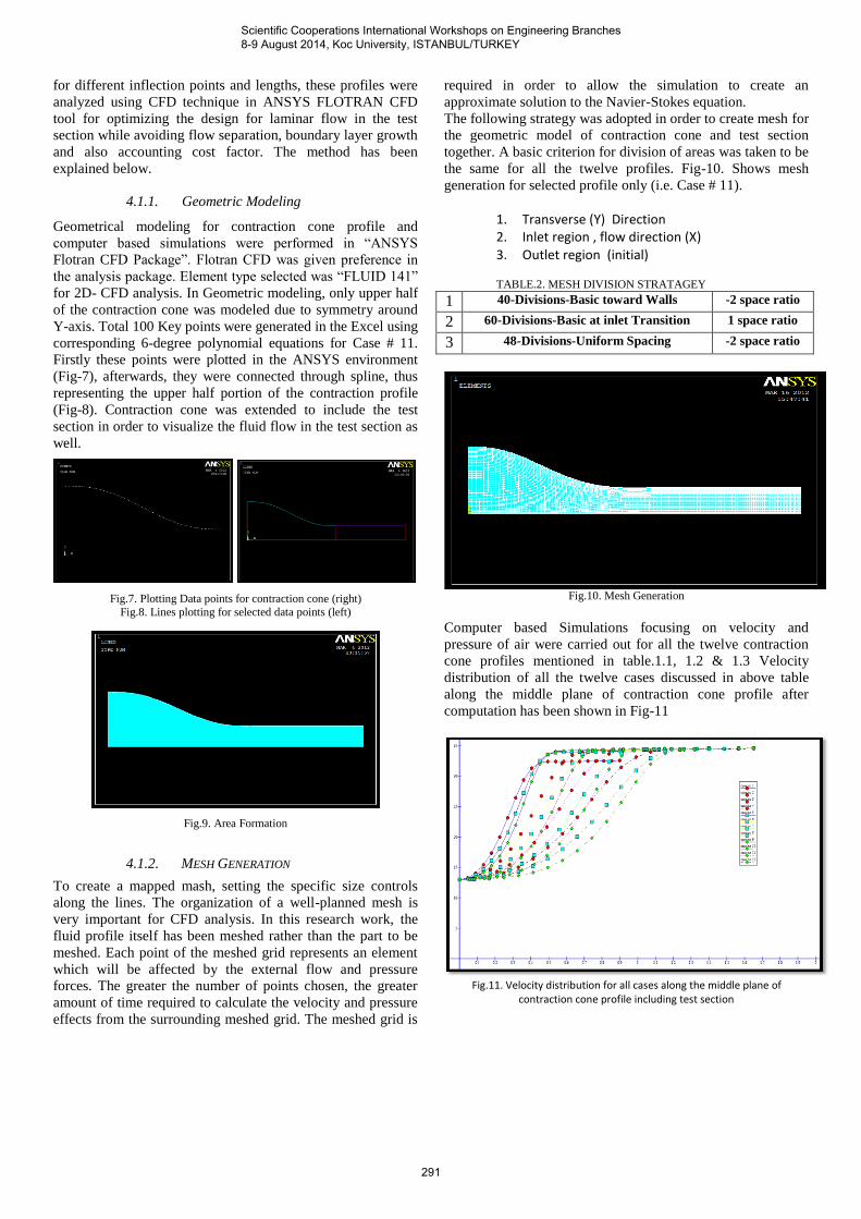
The following strategy was adopted in order to create mesh for

the geometric model of contraction cone and test section

together. A basic criterion for division of areas was taken to be

the same for all the twelve profiles. Fig-10. Shows mesh

generation for selected profile only (i.e. Case # 11).

1. Transverse (Y) Direction 2. Inlet region , flow direction (X) 3. Outlet region (initial)

TABLE.2. MESH DIVISION STRATAGEY

1 40-Divisions-Basic toward Walls -2 space ratio

2 60-Divisions-Basic at inlet Transition 1 space ratio

3 48-Divisions-Uniform Spacing -2 space ratio

Fig.10. Mesh Generation

Computer based Simulations focusing on velocity and

pressure of air were carried out for all the twelve contraction

cone profiles mentioned in table.1.1, 1.2 & 1.3 Velocity

distribution of all the twelve cases discussed in above table

along the middle plane of contraction cone profile after

computation has been shown in Fig-11

Fig.11. Velocity distribution for all cases along the middle plane of

contraction cone profile including test section


291

The simulations of all the twelve profiles have not been shown

due to unavailability of space. Velocity contour plot of

selected profile (i.e. case # 11) shown in Fig.13 and its

comparison with three others (i.e. case # 3,7 & 12) closer to

the results of case # 11 has been shown in Fig.15. All of these

simulations were based upon the following boundary

conditions. Boundary condition can be defined in either

preprocessing phase or in solution phase. In boundary

conditions, Degree of Freedom of the body was defined to

confine the flow. Velocity was applied at the inlet while value

of atmospheric pressure (absolute zero) was applied at outlet

of the contraction cone (Fig 12).

Fig.12. Applying Boundary Conditions

Fig.13. Velocity contour plot for selected profile

Variation of air velocity along the length of contraction cone

and test section has been shown in Fig- 14 where, distance is

taken along x-axis and velocity along y-axis. Following

solution options were provided in the solution phase.

• Steady state solution

• Laminar

• Adiabatic

• Incompressible

Number of global iterations was set to fifty. Post processing

was performed to infer the results like velocity and pressure

contours which were later compared to draw conclusions.

Fig.14. Velocity variation along wind tunnel length including contraction cone

& test section

From this activity, It was found that the best result, producing

uniform velocity profile at inlet to the working section, and

preventing separation of the flow within the contraction, was

obtained when the point of inflection was located as far

downstream as possible at a moderate length. Hence reducing

both flow separations within the contraction cone as well as

cost of the tunnel because of the moderate length. Therefore

best suited profile is for case # 11 with following

specifications.

Mathematical Model of Contraction Cone:

Contraction ratio=

Exit area=

Entrance area =

Inflection point =

Length =

Fig.15. Comparison of simulation of velocity profiles (velocity contour plot)


292

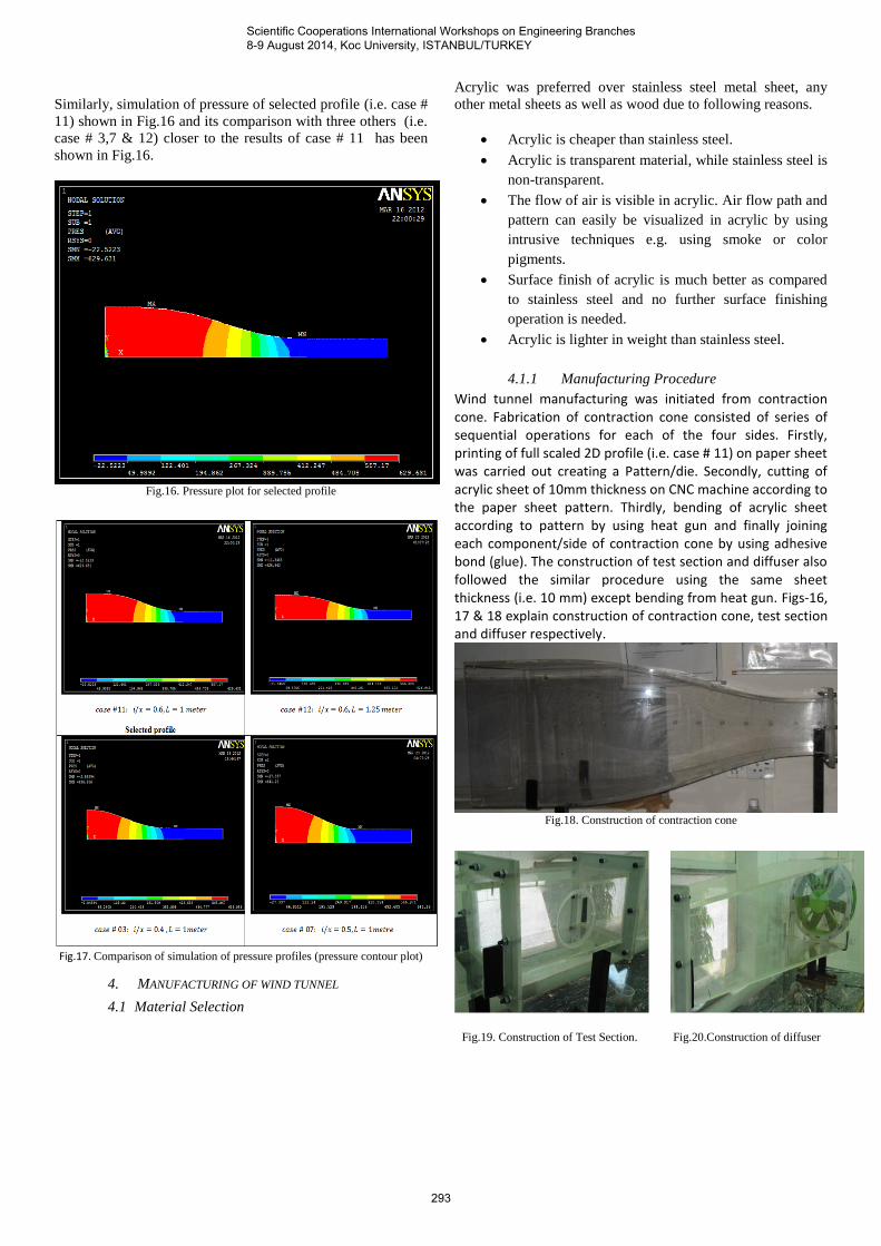
Similarly, simulation of pressure of selected profile (i.e. case #

11) shown in Fig.16 and its comparison with three others (i.e.

case # 3,7 & 12) closer to the results of case # 11 has been

shown in Fig.16.

Fig.16. Pressure plot for selected profile

Fig.17. Comparison of simulation of pressure profiles (pressure contour plot)

4. MANUFACTURING OF WIND TUNNEL

4.1 Material Selection

Acrylic was preferred over stainless steel metal sheet, any

other metal sheets as well as wood due to following reasons.

Acrylic is cheaper than stainless steel.

Acrylic is transparent material, while stainless steel is

non-transparent.

The flow of air is visible in acrylic. Air flow path and

pattern can easily be visualized in acrylic by using

intrusive techniques e.g. using smoke or color

pigments.

Surface finish of acrylic is much better as compared

to stainless steel and no further surface finishing

operation is needed.

Acrylic is lighter in weight than stainless steel.

4.1.1 Manufacturing Procedure

Wind tunnel manufacturing was initiated from contraction cone. Fabrication of contraction cone consisted of series of sequential operations for each of the four sides. Firstly, printing of full scaled 2D profile (i.e. case # 11) on paper sheet was carried out creating a Pattern/die. Secondly, cutting of acrylic sheet of 10mm thickness on CNC machine according to the paper sheet pattern. Thirdly, bending of acrylic sheet according to pattern by using heat gun and finally joining each component/side of contraction cone by using adhesive bond (glue). The construction of test section and diffuser also followed the similar procedure using the same sheet thickness (i.e. 10 mm) except bending from heat gun. Figs-16, 17 & 18 explain construction of contraction cone, test section and diffuser respectively.

Fig.18. Construction of contraction cone

Fig.19. Construction of Test Section. Fig.20.Construction of diffuser


293

4.1.2. Wind Tunnel Calibration

Wind tunnel calibration generally involved drilling holes at

mid-plane section of contraction cone and construction of

manometer. In order to measure pressure distribution in the

axial direction of contraction cone, 10 numbers of holes of

inner diameter 2mm and outer diameter 5mm at a mutual

distance of 0.1m (i.e.0.1m, 0.2, 0.3, 0.4, 0.5, 0.6, 0.7, 0.8, 0.9

& 1.0m) were drilled at mid-plane section. Pneumatic fittings

were placed afterwards in drilled holes.

Construction of manometer involved the following steps. A

wooden board of size 3 x 3 feet was selected and four pieces

of steel rods as well. Drilling of 10 holes of 1/8 in each piece

of steel rod was carried out. Plastic tubes 20 in numbers and

20 inches lengths were selected. The position of 4 rods was

marked on wooden board and rods were fixed on board by the

help of nuts and bolts. Pneumatic fittings were fixed on steel

rods Fig-19. Finally, fixing of plastic tubes in pneumatic

fittings was carried out to construct an inclined manometer as

shown in Fig-20. Colored water was used in order to visualize

and calculate pressure distribution.

Fig.21. Steel Tube with 10 pneumatic fittings (left)

Fig.22. Front view of Manometer (right)

Fig.21. Wind Tunnel in Assembled form

5. Experimental Results & Discussions

In the experimentation of wind tunnel, the design of

contraction cone was validated by comparing experimental

values of pressure & velocity of air obtained at different

sections i.e. 0.1 m apart along mid-section of contraction cone

length with computer based simulated values at corresponding

points during CFD analysis in ANSYS FLOTRAN.

Experimental values of velocities were measured indirectly

from pressures. Where, pressures were measured by

determining the height of water head in manometer and using

the following relation.

After calculating pressures, experimental values of velocities

were obtained from following equation as defined by [16]

Kailash Kotwani, Professor S K Sane and Dr. Hemendra Arya

[16].

----------(c)

Where

= 1000 kg/mᶟ at 25°C

= 1.182 kg/mᶟ at 25°C

The values thus evaluated have been shown in table 3

corresponding to different values of “X”.

TABLE.3. Pressure and Velocity at different points along mid-section of

contraction cone Length

It is evident from the results of pressure that variation in

simulated and experimental values is not more than 2 %. As

long as the velocity is concerned, the difference is observed

from X = 0 to 0.9 m consequently achieving the desired

velocity of about 35 m/sec at X=1.0 m (i.e. contraction cone

outlet/test section).It can be inferred from the results that, the

most possible reason of this difference is due to software

X

(meters)

Pressure

(Pa)

“Simulate

d Results”

Pressure

(Pa)

“Experimental

Results”

Velocity

(m/s)

“Simulate

d values”

Velocity

(m/s)

“Experimen

tal values”

0 21.154 19.554

13

8

0.1 20.148

19.554

13.077

8.1415

0.2 15.955

19.554

13.362

8.1415

0.3 6.0746

9.777

13.998

9.1025

0.4 -13.778

-9.777

15.182

10.77

0.5 -50.712

-39.108

17.154

13.6773

0.6 -116.76

-97.77

20.187

15.2314

0.7 -228.39

-215.094

24.432

20.757

0.8 -387.57

-342.195

29.34

24.083

0.9 -534.96

-508.404

33.072

29.914

1 -591.36

-586.62

34.276

34.7


294

limitation as the simulation resources were limited to 2D

analysis of the contraction cone profile for the wind tunnel due

Fig.22. Comparison of Experimental and Simulated values of velocities at mid

working plane

6. Conclusions & Future Aspects

Contraction cone design aimed at acquiring uniform and

steady stream at its outlet section and avoidance of flow

separation with a desired velocity (i.e. 35 m/sec).

Computational approach along with past research has been

used to select proper length and inflection point which are

known to be basic parameters for optimizing 2D-design of

contraction cone through velocity contour profile

investigation. The CFD analysis of velocity contour profile

authenticated and allowed the use of sixth order polynomial

equation for generating 2D-design of contraction cone which

was further analyzed and proved by experimentation after

construction and calibration of wind tunnel.

The main objective of constructing this wind tunnel was to

carry out experimentation on different types of airfoils in

laboratory. The current research may be extended to include

other parameters like flow visualization over test specimens of

different materials through smoke, installing six force sensors

for measurement of yaw, pitch and roll & automation of tunnel

for data Acquisition

7. References

1- WIND TUNNEL WIKIPEDIA

http://en.wikipedia.org/wiki/Wind_tunnel, “March,

2010”.

2- Craig A. Zehrug: “Comparative Analysis of a Low-

Speed Wind Tunnel Designed for Renewable Energy

Applications”. Purdue University Purdue e-Pubs

College of Technology Theses and Projects, Page-10,

2011.

3- WIND TUNNEL INDEX, NASA“

http://www.grc.nasa.gov/WWW/K-

12/airplane/shortt.html”, “Jan, 2011”.

4- Raymond L. Barger and John T. Bowen Langley: “A

GENERALIZED THEORY FOR THE DESIGN OF

CONTRACTION CONES AND OTHER LOW-

SPEED DUCTS”. Research Center Hampton, Va.

23365, Page-1 & 3A; November 1972.

5- R.D. Mehta and P. Bradshaw: “Technical notes of

design for small low speed wind tunnels” Reprinted

from the aeronautical journal of the royal

aeronautical society, Page-1, 445, 446 & 448;

November 1979.

6- Y James H. Bell and Rabindra D. Mehta:

“CONTRACTION DESIGN FOR SMALL LOW-

SPEED WIND TUNNELS”.Page-1 & 2; April 1988.

7- JONATHAN H. WATMUFF: “Wind tunnel

contraction design”. Gas dynamics laboratory,

department of mechanical and aerospace engineering,

Princeton University, Princeton, New Jersey 08544,

U.S.A, Page-1, December 1986.

8- Daniel Brassard: “Transformation of a polynomial

for a contraction wall profile”. Undergraduate

student, lakehead university, Ontario, Canada, Page-

1, Feb 24, 2003.

9- J.E. Sargison, G.J. Walker and R. Rossi: “Design and

calibration of a wind tunnel with a two dimensional

contraction”, Page-1, 2, 3 & 4; December 2004.

10- Frank M White: “Fluid mechanics” 7th edition, Page-

572.

11- Compressible flow Wikipedia.

http://en.wikipedia.org/wiki/Compressible_flow,

“April 2010”

12- Munson Young okiish: “Fundamentals of fluid

mechanics” 6th edition, Page-580.

13- “A vision in aeronautics” the wind tunnel project

white paper.

14- http://www.grc.nasa.gov/WWW/k-

12/WindTunnel/windtunnel_report.html,”April,

2010”

15- M. Abbaspour & M.N Shojaee: “Innovative approach

to design a new national low speed wind tunnel”,

Department of Mechanical Engineering Sharif

University of Technology and Graduate School of the

Environment & Energy, Science and Research branch

IAU, Tehran, Iran, 10 Dec. 2008.

16- Practices Manual for Low Speed wind Tunnel, TA-

50-250, Aerodynamic Tunnel EDIBON, S.A. c/ San

Jose 11-13, 28921-Alcorcon (Madrid) Espane.

17- Kailash Kotwani, Professor S K Sane and Dr.

Hemendra Arya: “Wind Tunnel Performance

Analysis (Measuring Power Requirement) Practical

Training Report”. Center for Aerospace System and

Design Engineering Department of Aerospace

Engineering Indian Institute of Technology, Bombay,

Page-9; August, 2003.


295

http://en.wikipedia.org/wiki/Wind_tunnel

http://www.grc.nasa.gov/WWW/K-12/airplane/shortt.html

http://www.grc.nasa.gov/WWW/K-12/airplane/shortt.html

http://en.wikipedia.org/wiki/Compressible_flow

http://www.grc.nasa.gov/WWW/k-12/WindTunnel/windtunnel_report.html

http://www.grc.nasa.gov/WWW/k-12/WindTunnel/windtunnel_report.html


296

Date post:	05-Jun-2018
Category:	Documents
Upload:	hoangdung
View:	225 times
Download:	0 times

Design & Construction of subsonic wind Tunnel focusing on...

Documents