Design, kinematics, and control of a soft - MIT...

Article

The International Journal of

Robotics Research

2016, Vol. 35(7) 840–869

� The Author(s) 2015

Reprints and permissions:

sagepub.co.uk/journalsPermissions.nav

DOI: 10.1177/0278364915587925

ijr.sagepub.com

Design, kinematics, and control of a softspatial fluidic elastomer manipulator

Andrew D. Marchese and Daniela Rus

Abstract

This paper presents a robotic manipulation system capable of autonomously positioning a multi-segment soft fluidic elas-

tomer robot in three dimensions. Specifically, we present an extremely soft robotic manipulator morphology that is com-

posed entirely from low durometer elastomer, powered by pressurized air, and designed to be both modular and durable.

To understand the deformation of a single arm segment, we develop and experimentally validate a static deformation

model. Then, to kinematically model the multi-segment manipulator, we use a piece-wise constant curvature assumption

consistent with more traditional continuum manipulators. In addition, we define a complete fabrication process for this

new manipulator and use this process to make multiple functional prototypes. In order to power the robot’s spatial actua-

tion, a high capacity fluidic drive cylinder array is implemented, providing continuously variable, closed-circuit gas deliv-

ery. Next, using real-time data from a vision system, we develop a processing and control algorithm that generates

realizable kinematic curvature trajectories and controls the manipulator’s configuration along these trajectories. Lastly,

we experimentally demonstrate new capabilities offered by this soft fluidic elastomer manipulation system such as enter-

ing and advancing through confined three-dimensional environments as well as conforming to goal shape-configurations

within a sagittal plane under closed-loop control.

Keywords

Flexible arms, mechanics, design and control, biologically-inspired robots, human-centered and life-like robotics,dexterous manipulation, manipulation

1. Introduction

Manipulators with rigid links and discrete joints provide

optimal solutions for automation, where fast, precise, and

controllable motions are utilized for repetitive tasks in

structured and often static environments; however, in natu-

ral environments and in human-centric operations, where

safety and adaptability to uncertainty are fundamental

requirements, soft robots may serve as a better alternative.

By studying a completely soft and compliant robot, we can

begin to identify appropriate hardware processes, kinematic

models, and control strategies for a growing class of robots

designed to incorporate softness.

In this work we present a completely soft spatial manip-

ulation system (see Figure 1). That is, we provide the

design, fabrication, and kinematic modeling of a new

manipulator morphology: a fluid-powered three-dimen-

sional multi-segment arm composed entirely of soft elasto-

mer. In addition, we develop a power system as well as

processing and control algorithms that enable autonomous

closed-loop control of the soft manipulator. We show how

the fluidic elastomer manipulator’s continuum kinematics

and soft material composition lead to several distinct advan-

tages when compared to traditional rigid body manipula-

tors. First, we show that the manipulator’s soft segments

deform according to constant curvature. With a constant

curvature assumption (Webster and Jones, 2010), we can

parameterize this N-link spatial soft manipulator with 2N

joint variables. Second, the kinematics and extreme compli-

ance of such a soft manipulator enable it to fit within and

advance through confined environments. When the bound-

aries of the environment can be parameterized by curved

cylinders and its curvature is non-zero, an idealized soft

fluidic elastomer manipulator will be more capable of

advancing through a confined environment than a

Computer Science and Artificial Intelligence Laboratory, Massachusetts

Institute of Technology, USA

Corresponding author:

Andrew D. Marchese, Computer Science and Artificial Intelligence

Laboratory, Massachusetts Institute of Technology, 32 Vassar Street,

Cambridge, MA 02139, USA.

Email: [email protected]

manipulator with rigid links and discrete joints. We demon-

strate this concept experimentally. Third, the continuum kine-

matics of a soft fluidic elastomer manipulator enable a high

degree of dexterity. Specifically, in an environment where a

collision-free path is parameterized by a curved path, the con-

tinuum kinematics of a fluidic elastomer manipulator can

generally fit the curvature of the path better than a rigid link

manipulator with discrete joints and rigid links.

Such new capabilities require innovation in both hard-

ware and modeling. The concept of using very soft elastic

materials to construct autonomous robots is relatively new

and radically different from the time-tested design and fab-

rication methodologies of traditional robotic systems. As

soft roboticists, we are in the process of defining long-

lasting morphologies for soft machines. Accordingly, a

considerable amount of innovation is required to design

functional soft machines, to develop processes by which

these machines can be repeatably fabricated, and to engi-

neer systems that drive their actuation.

1.1. A Review of soft manipulator designs

Soft machines have many distinguishing design character-

istics when compared to traditional hard robots. These dif-

ferences are reviewed by Trivedi et al. (2008). Soft robots

have continuously deformable backbones providing theore-

tically infinite degrees of freedom (DOFs). This attribute

classifies soft robots as a subclass of continuum robots, as

reviewed by Robinson and Davies (1999); however, not all

continuum robots are truly soft, and even continuum robots

referred to as soft have varying degrees of rigidity.

1.1.1. Discrete hyper-redundant manipulators. Before

reviewing the spectrum of continuum manipulator designs,

it is important to mention the discrete hyper-redundant

robot configuration. In contrast to continuum robots, this

configuration generally has a kinematically constraining

backbone composed of multiple rigid links serially con-

nected by revolute joints. Thus, this backbone has many

actuatable DOFs and approximates continuous body bend-

ing. Examples of discrete hyper-redundant robot manipula-

tors include the 32 DOFs elephant trunk manipulator

developed in Hannan and Walker (2003) and the 10 DOFs

snake arm robot developed in Buckingham (2002). Another

discrete hyper-redundant morphology is the variable geo-

metry truss manipulator (VGTM) as initially explored in

Miura et al. (1985) and Miura and Furuya (1988). These

designs also use discrete body links; however, here a link is

composed of two parallel prismatic joints held at the top

and bottom by rigid plates. Each of these body elements

resembles a parallel manipulator. A notable variable geome-

try truss manipulator is the planar prototype developed by

Chirikjian and Burdick (1994) with 10 body modules and

30 DOFs.

1.1.2. Hard continuum manipulators. As mentioned, con-

tinuum manipulators are realized through a spectrum of

morphologies. Many continuum manipulators are com-

posed of hard, but flexible material (e.g. materials having a

Young’s modulus of roughly 0.5 to 200 GPa). For example,

the elastic elephant trunk manipulator developed in Cieslak

and Morecki (1999) is composed of eight elastic elements

having coil spring backbones and is controlled as three

independent body segments yielding six DOFs. In addition,

Gravagne et al. (2003) and Gravagne and Walker (2002)

model and control the Clemson Tentacle Manipulator, a

hard continuum manipulator. This platform has two planar

sections, a total of four DOFs, and uses a spring steel back-

bone. Air-Octor developed in McMahan et al. (2005), the

articulated catheter robot developed in Camarillo et al.

(2009), and Tubot developed in Sanan et al. (2011) are also

examples of continuum manipulators constructed of hard,

but flexible materials. The aforementioned hard continuum

manipulators use tendons to control bending. Typically, an

array of servomotors or linear actuators are used to pull

cables that move connecting plates located between body

segments.

1.1.3. Semi-soft continuum manipulators. There are softer

continuum manipulator morphologies that use a combina-

tion of soft and hard components. In these designs, distribu-

ted pneumatic muscle actuators (PMAs) are most prevalent,

as the review by Trivedi et al. (2008) explains. OctArm IV

developed by McMahan et al. (2006) is a notable example.

This robot uses 18 PMAs distributed throughout four arm

segments yielding 12 DOFs. It is capable of adaptively

manipulating and grasping unknown objects that vary in

both size and shape (McMahan et al., 2006). Another

example is the continuum manipulator developed by Pritts

and Rahn (2004) that uses 14 PMAs within two body

Fig. 1. Soft fluidic elastomer manipulator gently taking a small

ball from the palm of its human collaborator. The manipulator’s

entirely soft composition and kinematic controller allow it to

safely interact with its environment. Reproduced with kind

permission from Mary Ann Liebert Inc. (Marchese et al., 2015a).

Marchese and Rus 841

segments yielding six DOFs. Also, the continuum manipu-

lator developed by Kang et al. (2013) uses 24 PMAs within

six body segments yielding 18 DOFs. Common features

among all these designs are rigid end plates to which the

PMAs are mounted and actuation pressures of between 50

and 100 psi. Accordingly, this manipulator morphology still

relies on rigid components and undergoes significant strain

stiffening, a phenomenon that adds rigidity to these robots.

1.1.4. Soft continuum robots. Constructing the body of a

continuum robot from soft elastic material likely began with

Suzumori et al. (1991) who developed pneumatically actu-

ated rubber segments capable of bidirectional bending.

These Flexible Microactuators (FMAs) were fiber-reinforced

and explored in the context of both a manipulator and multi-

fingered hand. More recently, soft roboticists have made

many notable low durometer rubber robots. For example,

several rolling belts have been produced by Correll et al.

(2010); Onal et al. (2011) and Marchese et al. (2011). Onal

and Rus (2013) emulated the serpentine locomotion of

snakes, Trimmer et al. (2006) and Umedachi et al. (2013)

emulated the peristaltic locomotion of caterpillars, and

Marchese et al. (2014c) and Katzschmann et al. (2014) emu-

lated the flapping propulsion of fish. Shepherd et al. (2011)

and Tolley et al. (2014) developed walking robots, and

Shepherd et al. (2013) developed a jumping robot.

1.1.5. Soft continuum manipulators. Recently, continuum

manipulators composed from soft elastic material have been

developed. These soft rubber manipulators can be categor-

ized under two primary morphologies. First, there are ten-

don driven arms consisting of variable length tendons,

typically cables or shape memory alloy wire, embedded

within and anchored to portions of a soft silicone arm. For

example, previous work on soft bio-inspired octopus-like

arms developed by Calisti et al. (2010) used tendons and

demonstrate capabilities like grasping (Laschi et al., 2012)

and locomotion (Calisti et al., 2011). Also, Wang et al.

(2013) developed a cable driven soft rubber arm consisting

of one large actuated segment that bends bi-directionally.

Lastly, McEvoy and Correll (2014) used a programmable

stiffness spine in conjunction with tendons to achieve shape

change in a soft rubber arm. The second morphology uses

fluidic elastomer actuators distributed among the manipula-

tor’s soft body segments. In short, this consists of embed-

ding independently actuatable agonistic fluidic channels

within each of the arm’s soft elastic body segments. When

fluid within these channels is pressurized, stress is induced

in the elastic body producing localized strain. This strain in

combination with a relatively inextensible backbone pro-

duces body segment bending. The primary advantages of

using fluidic actuation for soft continuum manipulators is

that this energy transmission system:

� can be lightweight making for easy integration into dis-

tal locations of the body;

� conforms to the time varying shape of the manipulator;

and� does not require rigid components to implement.

Deimel and Brock (2013) developed a pneumatically

actuated three-fingered hand made of reinforced silicone

that is mounted to a hard industrial robot and capable of

robust grasping. More recently, they have developed an

anthropomorphic soft pneumatic hand capable of dexterous

grasps (Deimel and Brock, 2014). In addition, we have pre-

viously shown planar manipulation is possible with an

entirely soft robot. That is, a six-segment planar fluidic

elastomer robot can be precisely positioned using a closed-

loop kinematic controller (Katzschmann et al., 2015;

Marchese et al., 2014a,b). Another relevant piece of work

is the manually operated three-dimensional elastomer tenta-

cles developed by Martinez et al. (2013) containing nine

pneumatic crescent-shaped channels (PneuNets) embedded

within three body segments.

1.1.6. Design contributions. However, the manipulator pre-

sented in this work differs from these prior works in several

important ways:

1. This arm is composed of 100% soft silicone rubber.

The arm is modular in both design and fabrication and

each module or arm segment has four fluidic actuators

and moves in three spatial dimensions.

2. The manipulator has features such as a hollow cylind-

rical interior and soft segment endplates. The hollow

interior accommodates fluid transmission lines and

allows modular assembly. Markers placed on segment

endplates allow an external vision system to capture

the segment endpoint positions. Both of these features

are essential to an autonomous manipulation system.

3. The arm has a longitudinally tapering clover-shaped

exterior and this morphology has a significant impact

on the manipulator’s dynamics (Marchese et al.,

2015b).

1.2. A Review of soft manipulator kinematics

1.2.1. Robot-independent model. Despite the variability in

continuum manipulator designs, their kinematics can often

be represented using a piece-wise constant curvature (PCC)

model. This is the message within a 2010 review of conti-

nuum robots by Webster and Jones (2010). That is, Webster

and Jones review several seemingly distinct kinematic

modeling approaches, but show that when using a PCC

modeling assumption, these approaches yield identical

robot-independent results. This assumption means each

body segment of a multi-segment arm is assumed to deform

with constant curvature. An early use of PCC modeling

appears in Hannan and Walker (2003) where a bending

robotic trunk is developed.

842 The International Journal of Robotics Research 35(7)

Again as Webster and Jones (2010) describe, the trans-

formation from configuration space consisting of arc length

L, curvature k, and plane orientation g (see Figure 2) to

task space consisting of Cartesian position and orientation

or pose can be derived in multiple ways. Differential geo-

metry (Hannan and Walker, 2003) or the use of virtual links

and a Denavit–Hartenberg approach (Jones and Walker,

2006a) are among a few of the derivations. The robot-

independent forward kinematic transformation for a single

continuum segment is

T=

cosg cosks � sing cosg sinkscos g(1�cos ks)

k

sing cosks cosg sing sinkssin g(1�cosks)

k

� sinks 0 cosks sinksk

0 0 0 1

26643775

where s = [0, L]. Although the PCC modeling assumption

is quite powerful, it does not always apply to continuum

manipulators. The obvious limitation being that not all con-

tinuum robots deform according to segmented constant cur-

vature. A common exception is when a continuum body

segment assumes a spiral, i.e. curvature increases from the

segment’s base to tip. Mahl et al. (2013) develop general

variable curvature continuum kinematics for this reason.

Giorelli et al. (2012) develop forward and Jacobian based

inverse kinematics for a planar conical soft manipulator that

again spirals. Accordingly, an important contribution of this

work is that we validate this PCC modeling assumption in

the context of a soft fluid-powered elastomer manipulator.

1.2.2. Robot-dependent model. A robot specific mapping

is required from actuation space (e.g. tendon lengths or

pressures) to configuration space (i.e. L, k, and g) as

reviewed in Webster and Jones (2010). Previous work on

continuum robots has generally approached this robot

dependent mapping or model in three ways.

First, Gravagne et al. (2003), Webster et al. (2009) and

Trivedi et al. (2008) use Bernoulli–Euler beam mechanics

to predict the deformation of continuum robots. When a

beam is subject to a tip moment, the beam moment Mb

along the length l is constant, Mb(l) = c, and it deforms

under constant curvature, k = Mb/(EI). A common realiza-

tion of this is an actuator parallel to the beam’s neutral axis

that applies a load to a fixture mounted orthogonal to the

beam at the tip. This modeling approach does not apply to

our device as it has a fundamentally different operating

principle: the soft segment stores bending energy in its out-

ermost actuated layer as opposed to its inner backbone. If

the inner layer is assumed to store bending energy, and the

Bernoulli–Euler beam model is applied, a non-constant

moment along the backbone is predicted producing non-

constant deformation.

Second, continuum robots with high pressure (50–100

psi max) (McMahan et al., 2006; Kang et al., 2013;

Suzumori et al., 1991) and medium pressure (30 psi max)

(Chen et al., 2006) PMAs as well as tendons and cables

(Jones and Walker, 2006b; Hannan and Walker, 2003;

McMahan et al., 2005; Wang et al., 2013) first make the

assumption that segments are deforming under constant

curvature and second make the assumption that actuators

either lengthen or shorten as a function of input.

Subsequently, a relationship between joint variables, i.e.

three or four actuator lengths, and constant curvature arc

parameters are developed. This approach does not gener-

ally apply to our device as the low durometer rubber com-

position and lack of kinematic constraints means our

actuators are expanding spatially at varying rates, not only

expanding axially.

Lastly, and perhaps most relevant are robot specific

models developed to understand the deformation of

extremely soft low pressure fluidic actuators. Onal et al.

(2011) develop a static analytical model under the condi-

tions of:

� only longitudinal strain;� uniform rectangular channels with square cross-

sections orthogonal to the bending axis� a rectangular actuator shape; and� and stresses that are based on initial channel geometry.

Marchese et al. (2014c) extend this approach to analytical

modeling and account for unequal radial and longitudinal

strain as well as non-uniform square channels orthogonal

to the bending axis. Shepherd et al. (2011) develop a model

that assumes equal longitudinal and radial strain in uniform

round channels orthogonal to the bending axis in a rectan-

gular actuator and use a linear stress-strain relationship.

These models all assume a two-dimensional cross-section

of infinite thickness.

1.2.3. Modeling contributions. An important contribution

of this work is that we show the viability of the PCC model-

ing assumption in the context of a spatial fluidic elastomer

manipulator. We also develop a static deformation model

that suggests with uniform initial channel geometry and no

external loads, the actuated region of the developed soft

x

y

z

κ-1

L

γ

•Fig. 2. Arc parameters arc length L, curvature k, and plane

orientation g used to model the bending of a spatial continuum

segment under the PCC assumption. This figure is adapted from

Webster and Jones (2010).


segments will deform under constant curvature. This differs

from the above related work in the following ways.

1. It describes the deformation of a soft fluidic actuator

that is a non-uniform cylindrical shape, operates at low

pressures, and has a non-uniform cylindrical channel

along the bending axis subject to unequal longitudinal

and circumferential strain.

2. It accounts for the stress changing as a function of

deforming channel geometry and is more valid for

large deformations.

3. The model uses nonlinear material properties.

1.3. Overall contributions

Specifically, this paper contributes a novel autonomous

three-dimensional fluidic elastomer manipulator. That is,

we provide the following:

(a) a novel multi-segment manipulator prototype, (i) con-

structed 100% from soft silicone rubber, (ii) powered

by four fluidic elastomer actuators per segment, and

(iii) designed with a modular morphology suitable for

automation;

(b) a novel process to repeatably fabricate this

manipulator;

(c) a novel static model to understand a segment’s

deformation;

(d) a multi-segment kinematic model and processing and

control systems that enable the first autonomous cap-

abilities for this manipulator type, e.g. (i) following

configuration trajectories within a sagittal plane and

(ii) positioning in three-dimensions; also, without

using the model and control system, we demonstrate

(iii) advancing through a confined environment; and

(e) evaluations in both simulations and physical

experiments.

This paper is organized as follows. In Section 2 we

provide an overview of the aggregate soft fluidic elasto-

mer manipulation system and introduce the major subsys-

tems (i.e. actuation, perception, power, and processing

and control). Section 3 presents the design, modeling, and

fabrication of the soft spatial fluidic elastomer manipula-

tor. Specifically, Section 3.1 describes the arm’s morphol-

ogy and Section 3.2 details alternative designs. In Section

3.3, we develop and experimentally validate a robot-

dependent kinematic mapping to understand the deforma-

tion of the manipulator’s individual segments as well as a

multi-segment kinematic model based on the PCC

assumption (Webster and Jones, 2010). In Section 3.4, we

detail the fabrication process for the soft arm, which is a

three-dimensional extension of a fabrication process the

authors developed to construct a two-dimensional soft

manipulator presented in Marchese et al. (2014a). Section

4 details the development of a high capacity fluidic drive

cylinder array used to power actuation. Section 5 provides

a kinematic control algorithm for both measuring the

arm’s configuration and autonomously driving the arm to

a user-specified target shape configuration. In Section 6

we explore new capabilities enabled by these above devel-

opments. We demonstrate how the kinematics and

extreme compliance of such a soft manipulator enable it

to fit within and advance through confined environments

in Section 6.1. Next, we demonstrate how the continuum

kinematics combined with our approach to closed-loop

shape control enable the arm to conform to arbitrary con-

figurations in real-time in Section 6.2. Lastly, in Section

6.3 we demonstrate it is feasible to position the soft flui-

dic elastomer manipulator in three dimensions.

2. System overview

The soft fluidic elastomer manipulation system can move in

three dimensions and is subject to gravity. The aggregate

system is depicted in Figure 3 and contains actuation, per-

ception, power, and computation subsystems. A fluidic

elastomer arm composed entirely from soft silicone rubber

is suspended (Figure 3(a)). Each of the manipulator’s four

body segments (Figure 3, 1–4) are independently actuatable

with two bending DOFs and is fabricated through a multi-

step casting process. The arm attaches to a grounded frame

by means of a rotary stage at its base (Figure 3(b)). A bun-

dle of transmission lines (Figure 3(d)) carries pressurized

fluid from an array of fluidic drive cylinders (Figure 3(e)),

or pumps, to actuated channels that are distributed through-

out the arm. A system of cameras (OptiTrack; NaturalPoint,

Inc., Corvallis, OR) (Figure 3(c)) is used to localize mar-

kers on the soft connectors between the arm’s body seg-

ments. The computational subsystem (Figure 3(f)) uses

kinematic algorithms and cascaded controllers to provide

closed-loop curvature control of the manipulator. The sub-

system determines the arms measured representation and

target configurations as well as sends control signals to the

fluidic drive cylinders.

3. Actuation

3.1. Soft manipulator design

The soft spatial manipulator is composed entirely from low

durometer silicone rubbers and is actuated by pressurizing

fluid channels embedded within the arm. The 50 cm long

600 g arm, shown in Figure 4(a), is composed of indepen-

dently casted and serially concatenated modular segments

that each move in three spatial dimensions with two DOFs.

The arm is held horizontally from its midpoint subject to

gravity emphasizing the manipulator’s high body compli-

ance in Figure 4(b). The durability of such an entirely soft

design is shown in Figure 4(c)a (e) as well as in Media

Extension 1. These demonstrations are inspired by the resi-

liency tests that Tolley et al. (2014) use in the evaluation of

a soft walking robot. The arm remains functional in

extreme heat and in underwater environments while the


actuation system is placed external to the extreme condi-

tion. In addition, after being subjected to large compressive

loads, the arm resumes normal operation. The same robot

prototype used in these durability tests was used to perform

all 42 reported experimental evaluations in the following

sections. In total, this prototype withstood several hundred

experimental evaluations.

The morphology of our spatial manipulator draws

inspiration from previous work. The soft rubber tentacles

developed by Martinez et al. (2013) use embedded pneu-

matic actuators in a similar two layer rubber construction.

In addition, inspiration is drawn from a planar manipulator

developed by the authors in Marchese et al. (2014a); how-

ever, the manipulator presented here differs from these

works in several ways. Firstly, similar to our planar arm,

this manipulator is modular in both design and fabrication;

however, the spatial morphology differs in that each mod-

ule or arm segment has four distributed fluidic actuators

allowing it to move in three spatial dimensions. Secondly,

similar to our planar design, but different from the design

in Martinez et al. (2013), the manipulator presented here

has features such as a hollow cylindrical interior and soft

segment endplates. The hollow interior accommodates fluid

transmission lines and allows modular assembly. The soft

endplates contain markers allowing an external camera sys-

tem to localize their positions. Both features are essential

to an autonomous manipulation system. Thirdly, the arm

has a longitudinally tapered and clover-shaped exterior (see

Figure 5(b)) and this has a significant impact on the manip-

ulator’s dynamics (Marchese et al., 2015b) because of the

reduced mass of the distal segments.

In Figure 5B, a schematic of the spatial manipulator is

shown and as mentioned before, this manipulator is com-

posed of four tapering segments separated by soft segment

connectors (Figure 5(g)). Figure 5A depicts the two layer

concentric structure of a segment. The outer layer (Figure

5(e)) is made from a very soft silicone rubber and the inner

layer (Figure 5(d)) is made from a slightly stiffer silicone

rubber. Within the outer layer of the segment, four cylindri-

cal fluidic channels (Figure 5(c)) are embedded along the z

-axis and are spaced at 90 intervals. These channels enable

the arm to bend in two orthogonal planes. When a channel

Fig. 4. (a) The soft spatial manipulator . Reproduced with kind

permission from the IEEE (Marchese et al., 2015b); (b) the arm

is suspended horizontally from its midpoint subject to gravity

illustrating its high body compliance; (c) the arm is operated

on the surface of a grill measuring 230�C; (d) the arm is

operated under water; and (e) the arm is run over by a 4,000 kg

truck at approximately 5 mph and afterwards resumes normal

operation.

Fig. 3. Overview of the spatial fluidic elastomer manipulation system. The system consists of (a) soft spatial manipulator composed

of four body segments, (b) rotary stage, (c) a system of cameras for external perception, (d) fluid transmission lines, (e) fluidic drive

cylinders, and (f) processing and control algorithms.


is pressurized with fluid, the outer layer undergoes both

longitudinal and circumferential strain; however, the inner

layer is designed to be inextensible under the induced stres-

ses and this difference in material strain results in bending

about the inextensible z -axis. Bending motion primitives

are shown in Figure 5(c). Combining actuation in the x and

y directions allows for bending in any direction with zero

rotation around the longitudinal axis. Alternatively, a tradi-

tional rotational DOF can be introduced at the segment’s

base to define g and a single channel can be actuated to

define k. To achieve three-dimensional positioning, but to

prevent the segments from twisting about their neutral axis

(an unactuated DOF), in this work we actuate the manipu-

lator in a sagittal plane defined by the rotation of a stage to

which the base connector (Figure 5(b)) is mounted. Each

segment’s center is hollow and used to accommodate

internal fluid transmission lines (Figure 5(a)) that function

to deliver pressurized fluid to each actuated channel as well

as facilitate the concatenation of multiple segments. On

one end, each transmission line is individually connected to

each actuated channel in the multi-segment arm by means

of a crush resistant silicone insert (Figure 5(f)) shown in

red. These inserts are created from relatively stiff pieces of

silicone tubing. On the other end, each line connects to the

outlet of a fluidic drive cylinder, a device originally devel-

oped by the authors in Marchese et al. (2014b).

3.2. Alternative designs considered

To arrive at the current entirely soft manipulator design, we

evaluated many alternative designs with varying degrees of

rigidity. Through an iterative process, we were able to

Fig. 5. (A) A cross-section in the x–y plane details the concentric layered structure of the manipulator’s soft segments. (B) A

schematic of the four segment spatial manipulator implemented in this work with the following components: (a) fluid transmission

line bundle, (b) base connector, (c) expansion channels, (d) inner layer, (e) outer layer, (f) crush resistant channel inlet, and (g)

segment connector. (C) The actuation motion primitives of a single soft segment: A segment bends through pressurization of the

embedded fluidic channels.


design away all non-rubber components. For example,

Figure 6 illustrates several of these past design alternatives.

In Figure 6(a), a semi-soft manipulator is shown and it is

composed of several arm segments each consisting of a

plastic backbone and metal ribs surrounded by casted rub-

ber (Figure 6(b)). Figure 6(c) shows one of these kinemati-

cally constrained soft segments under actuation. In this

design iteration, the manipulator’s endplates were rigid, and

without a hollow interior, fluid transmission lines were run

external to the manipulator. These lines interfered with the

vision system’s ability to measure marker locations as well

as the manipulator’s mobility. In addition, the arm segments

shown here are cylindrical and uniform along the length of

the manipulator producing a larger suspended mass than

the current design. Figure 6(d) shows a second alternative

design where a plastic helix was introduced around the seg-

ment’s exterior. Noticeably, although this kinematic con-

straint reduced circumferential strain, it produced torsion

about the neutral axis under actuation (Figure 6(e)).

3.3. Kinematic modeling

In order to autonomously perform tasks with the manipula-

tor developed in Section 3.1, we must develop a multi-

segment kinematic model. The objectives of this section

are to:

(a) understand how an individual body segment deforms

under fluidic input;

(b) determine what simplifying assumptions can be made

in order to create a multi-segment kinematic model;

and

(c) experimentally evaluate the proposed kinematic

model.

An important result is that we use and validate a PCC mod-

eling assumption (Webster and Jones, 2010), explained in

Section 1.2, to describe this multi-segment soft manipula-

tor. The PCC-based kinematic model developed here will

be used by a controller, detailed in Section 5, to regulate the

manipulator’s configuration in real-time.

3.3.1. Segment deformation. In this section we extend an

analytical modeling approach presented by the authors in

Marchese et al. (2014c) to understand how one of the

manipulator’s soft arm segments deforms. Although this

deformation model is not utilized for any part of the con-

troller, it is used as an analytical design tool for under-

standing how input pressure as well as physical actuator

properties result in segment deformation. This simplified

deformation model suggests that a significant portion of

the actuator will deform under approximately constant cur-

vature. Based on this observation, we use a simpler PCC

model (see Section 3.3.5) to represent the manipulator’s

forward kinematics during control.

Figure 7 provides a schematic representation of a soft

arm segment in both a neutral state (Figure 7(a)) and a

deformed state (Figure 7(b)). In addition, Figure 7(c) illus-

trates an isometric view of a thin slice of the segment’s

elastically deformed outer layer.

The segment bends due to the relative difference in stiff-

ness between the inner and outer rubber layers. The inner

layer is cast from a rubber chosen to have an elastic modu-

lus approximately 5.5 times greater than that of the outer

layer, allowing us to make the assumption that the inner

layer is inextensible relative to the outer layer. In addition,

the outer layer thins considerably, further reducing stiffness.

By pressurizing the fluidic channel embedded within the

outer layer, stress is induced both circumferentially (normal

to the neutral z-axis) and longitudinally (parallel to the neu-

tral z-axis) in the outer layer, resulting in circumferential

expansion and longitudinal elongation respectively. Due to

the difference in lengths between the inner and outer layer,

the segment bends.

Fig. 6. Example design alternatives having varying degrees of rigidity. Through an iterative design process, all non-rubber

components were removed.


In order to understand how a segment bends, we consider

the case of one of the segment’s channels deforming under

pressure. Our approach is to first model the deformation of

this channel as a function of the channel’s fluid pressure pc.

The model is based on dividing the channel into J cross-

sectional slices of uniform z-axis length cut parallel to the

x–y plane and calculations are performed independently on

each slice. In general, a bar (�) is used to described an ini-

tial, undeformed channel dimension, whereas a hat ( ) is

used to describe a deformed channel dimension. Then, to

simulate segment bending, we iteratively apply this model

each time increasing pc. More specifically, at each iteration

the channel’s circumferential and longitudinal deformed

dimensions are recalculated based on the material stresses

that are derived from the previous iteration’s deformed geo-

metry. The model’s input pressure pc is not linearly

increased, rather it is measured during a physical experi-

ment where an actuator is incrementally filled under vol-

ume control (see Section 3.3.6). The motivation behind

using this measured data as input is that it accounts for

nonlinearities observed in the segment’s pressure profile.

Figure 8(a) depicts the bending of the inextensible layer

predicted by the simulation as well as a priori channel pres-

sure data that was successively input into the simulation at

each iteration. Also, the measured, and the model predicted,

accumulated bending angle u is shown at each iteration.

Figure 8(b) is a photograph of the actual segment that the

model is based on at the maximum pressure used in the

Fig. 7. Schematic representation of a soft arm segment under deformation.

Fig. 8. (a) Left-hand side: neutral axis bending of the soft arm segment whose physical parameters are listed in Table 1 is simulated.

Middle: details a priori channel pressure data successively input into the simulation each iteration. Right-hand side: the resulting

model predicted and measured accumulated bending angle u. (b) A photograph of the modeled segment at the maximum pressure

used in the simulation.


simulation and experiment. Table 1 lists important model

and simulation parameters.

3.3.2. Stresses and strains. Stresses and strains in the elas-

tomer can be approximated at a simulation iteration given

the channel’s current deformed geometry as well as the

pressure input. After these stresses and strains are com-

puted, they can be used to update the channel’s deformed

geometry for the next simulation iteration. First, we find

the material stresses. Due to the fact that each of the seg-

ment’s embedded channels are cylindrical, we can approxi-

mate the circumferential stress sc in a thin cross-sectional

channel slice by balancing static forces. That is, the pres-

sure force acting to circumferentially expand the channel

should balance with the product of circumferential wall

stress and wall area (see Figure 7(c) for visualization)

2 sciti ~wi ’ pc

hi�1 + hi

2~wi 8 i = 1, . . . , J ð1Þ

sci’pc

hi�1 + hi

4 ti

8 i ð2Þ

When the condition hi�1 = hi is met,

sci’pc

hi�1

2 ti

8 i ð3Þ

In the above approximations, i is the slice index, J is the

total number of slices, pc is the channel’s fluid pressure,

and h, w, and t are a slice’s deformed channel diameter, dis-

tal wall length, and wall thickness, respectively. The dimen-

sion ~w represents the slice’s deformed wall length midway

through the slice (see figure 7(c)).

Using a similar approach to determining the circumfer-

ential stress, we can approximate the longitudinal stress sL

in a slice as

sLi’

pc h2i�1

4b ti ti + hi�1

� � 8 i = 1, . . . , J ð4Þ

To arrive at the above approximation (equation (4)), we

include a free parameter b allowing the stress to be adjusted

such that the model predictions better match experimen-

tally observed deformations. It is important to note that this

is the only free parameter in the model. We use b = 4 and

justify this by using the fact that the inner most portion of

the channel wall is laminated to an inextensible surface,

counteracting a significant portion of the applied pressure

force. An important insight from this is that the longitudi-

nal stress is predicted to be approximately one eighth of

the circumferential stress.

Next, the circumferential and longitudinal strain, ec and

eL respectively, can be determined using a look-up table

based on the material’s measured true stress true strain rela-

tionship, shown in Figure 9.

3.3.3. Updating channel geometry. Having determined the

material’s strain, we can now update the deformed dimen-

sions of a channel slice under the increased pressure. That

is, the elongated wall w, the expanded diameter h, and com-

pressed thickness t can be expressed using the calculated

material strain, the initial channel geometry (represented by�h, �w, and �t), and the conservation of material volume as sili-

cone rubber is incompressible. The dimension w is updated

according to

wi’�wi eLi+ 1ð Þ 8 i ð5Þ

The updates for h and t can be found by solving a system

of two equations. Equation (6), is found using the previ-

ously determined circumferential strain,

hi’ci

p� t 8 i ð6Þ

where

ci’�ci eci+ 1ð Þ ð7Þ

�ci = p �hi +�ti� �

ð8Þ

The dimensions �c and c represent the undeformed and

deformed channel circumference measured half-way

through the wall’s thickness. Equation (9), is found using

the conservation of material volume. That is, the initial

Table 1. Segment parameters used in the simulation.

Parameter Symbol Value

Segment length L + 2LP 9.7 cmChannel length L 7.1 cmNumber of slices J 15Slice wall length �w = L

J0.47 cm

Channel diameter, �h 0.32 cmChannel wall thickness �t 0.32 cmSimulation iterations 10

0 0.5 1 1.5 20

0.1

0.2

0.3

0.4

0.5

0.6

ε

σ [M

Pa]

Fig. 9. True stress true strain relationship of the rubber material

composing a segment’s outer layer.


volume of elastic material in a slice is equal to the volume

of material in the slice when it is deformed

�Ai �wi’Ai �wi + Ai

wi � �wi

28 i ð9Þ

where �A and A are the initial and deformed cross-sectional

area of a slice, respectively. More specifically

�Ai = p�hi

2+ �ti

� �2

�p�hi

2

� �2

8 i ð10Þ

Ai = phi

2+ ti

!2

�phi

2

!2

8 i ð11Þ

According to the technique outlined in the actuation section

of Marchese et al. (2014c), the accumulated angle u along

the neutral axis at this simulation iteration is

u =XJ

i = 1

cos�1 �w2i + h2

i�1 + �w2 + h2i

2hi

ffiffiffiffiffiffiffiffiffiffiffiffiffiffiffiffiffiffiffih2

i�1 + �w2

q0B@

1CA� tan�1 �w

hi�1

� �ð12Þ

3.3.4. Conditions for constant curvature. From this model

we can make the following observation: if the initial unde-

formed channel dimensions are constant along the length of

the channel, i.e.

�wi = C1 8 i = 1 . . . J ð13Þ�hi = C2 8 i ð14Þ�ti = C3 8 i ð15Þ

then the deformed dimensions w, h, and t and accordingly

the bending angle u are constant 8 i = 2, . . . , J � 1 along

the length of the channel.

It is important to note that under these simplified condi-

tions, only the actuated region of the segment, i.e. the chan-

nel with arc length L (see Figure 7), is expected to deform

under constant curvature; both the channel inlet region as

well as the channel occlusion region contribute non-

constant curvature effects to the aggregate segment’s bend-

ing profile because of the increased stiffness in these

regions. To account for this, linear transformations are

added before and after the constant curvature transforma-

tion in equation (16) within Section 3.3.5.

3.3.5. Segment transformation. Given that a channel

deforms under approximately constant curvature, we can

write the following transformation from the base of a seg-

ment to the tip

Sbasetip =Rz gð ÞTz LPð ÞRy

u

2

� �Tz d uð Þð ÞRy

u

2

� �Tz LPð Þ

ð16Þ

Here, T and R represent coordinate translations and rota-

tions along and about the subscript axes; refer to Figure 7

for coordinate definitions. The center three transformations

are consistent with kinematic representations of continuum

manipulators, and are used when the constant curvature

assumption is valid (Webster and Jones, 2010). In the con-

text of this work we need to add additional translations

along z before and after the bent channel to account for the

relative rigidity of the inlet pieces. In addition, we redefine

d(u) with an approximation that is singularity free for the

reason of numerical stability

d uð Þ= 2 L

usin

u

2

� �ð17Þ

d uð Þ’L a u2 � 1� �

ð18Þ

where a is a fitting coefficient. An important observation is

that the segment transformation Sbasetip has two DOFs. That

is, if we know the sagittal plane along which the segment is

bending, specified by g, and are given one point along the

segment’s neutral axis in reference to the segment’s base we

can uniquely define u. In addition, in order to specify a

point along the neutral axis of the curved region s = [0, L]

in reference to the base of the channel we use the following

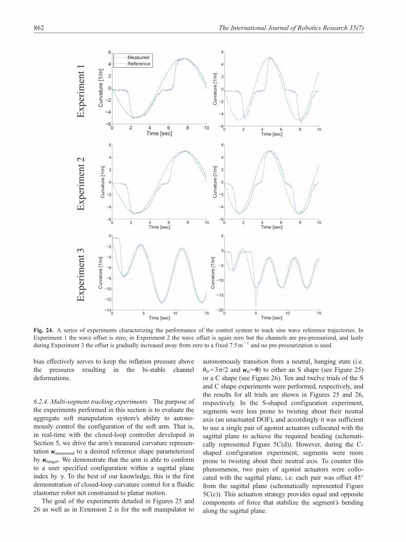
transformation

Sbases =Rz gð ÞTz LPð ÞRy

k s2

� �Tz d k sð Þð ÞRy

k s2

� �k = u

L

ð19Þ

The kinematics of a multi-segment soft arm composed of N

segments can be represented by cascading single segment

transformations together

MbasetipN

=Sbasetip g1, u1ð ÞSbase

tip g2, u2ð Þ � � � Sbasetip gN , uNð Þ

ð20Þ

3.3.6. Model evaluations. In order to validate this kine-

matic model we fabricated and actuated the segment

described physically in Table 1 subject to gravity. The seg-

ment weighs 65 grams. The primary concept we are evalu-

ating in this experiment is: if we identify a single point on

the arm segment, i.e. the tip, and the segment’s base posi-

tion and orientation is known, then we can uniquely define

the entire segment’s neutral axis. The experiment consists

of incrementally filling a single channel with between 0

and 70 ccm of air and photographing the segment’s defor-

mation. As a metric of goodness of fit, we compare our

models predicted bending angle uP with the measured

bending angle uM at each incremental fill level. In addition,

we compare our models predicted center of gravity GP with

the measured center of gravity GM. Measurements were

taken along the neutral axis of the segment using image

analysis. uM was measured from the unbent tip region and

GM was taken to be at s = L/2, the center point of the neu-

tral axis. The model is defined using a single point, in this

case the segment’s tip. Figure 10(a) shows the test segment


being incrementally filled from 32 to 72 ccm of air. Table 2

contains a comparison between measured and model pre-

dicted deformation kinematics.

In addition, we performed the same experiment on a

segment weighing 173 grams under the external load of an

attached second segment weighing 85 grams. The intent of

this experiment was to quantify the error in the proposed

kinematic segment model when the segment is under sig-

nificant external load. For the same volumetric input, the

maximum measured bending angle of 40� is significantly

smaller than in the unloaded case, 123�. As expected, the

error in the model predicted bending angle is higher in the

loaded case than in the unloaded case and in the loaded

case the error increases with gravitational loading. Within

the range 640� the error does not exceed 7.0�, with a mean

of 2.7�. Figure 11 depicts the percent error in the prediction

as a function of measured bending angle. Generally, as

bending angle increases the error in predicted bending

angle grows. Figure 10(b) shows the loaded test segment

being incrementally filled from 32 to 72 ccm of air.

3.3.7. Limitations. The static deformation model is most

valid for describing the soft segment’s deformation at larger

Fig. 10. Experimental validation of the proposed segment transformation. (a) A single segment is incrementally filled with air in the

sequence of images (A–F). (b) A larger soft segment is actuated in the image sequence (A–F) with the suspended weight of a second

distally attached segment.

Table 2. Comparison between the measured and the model predicted deformation kinematics.

Fig 10(a) Volume (ccm) Pressure (kPa) uP (�) uM (�) |GP 2 GM| (cm)

(F) 72 40.6 121 122.5 0.54(E) 64 39.0 104 105.6 0.45(D) 56 35.7 83 83.6 0.48(C) 48 32.8 61 61.4 0.30(B) 40 31.5 39 40.2 0.20(A) 32 29.7 16 13.8 0.24

Table 3. Comparison between measured and model predicted deformation kinematics for segment under external load

Fig 10(b) Volume (ccm) Pressure (kPa) uP (�) uM (�) |GP 2 GM| (cm)

(F) 72 40.6 33.1 39.9 0.30(E) 64 39.0 28.3 34.5 0.18(D) 56 35.7 24.4 28.1 0.12(C) 48 32.8 19.2 20.5 0.03(B) 40 31.5 14.6 15.3 0.09(A) 32 29.7 9.9 10.0 0.08- 24 23.0 4.3 3.7 0.09


bend angles. At lower pressures, the model predicted and

measured bend angles deviate significantly. This is likely

because the presented model does not capture the bi-stable,

nonlinear channel deformation encountered when inflating

a thin-walled elastomer tube (detailed in Gent (2012)). A

more detailed explanation of this phenomenon and how it

relates to the actuator’s performance can be found in

Section 6.2.3. However, it is possible that by adjusting the

model’s free parameter b at each iteration, such nonlinear

behavior can be more closely approximated.

A notable limitation in our experimental evaluation of

the developed kinematic model is that we do not directly

establish the validity of the PCC-based model’s ability to

describe the backbone’s continuous deformation; rather we

experimentally validate the model’s ability to describe the

segment’s aggregate bend angle and center of mass loca-

tion, which are indirectly a function of the continuous

deformation.

In addition, the developed soft segments have physical

limitations. For example, they are inherently force limited

and this impacts the maximum achievable bend angle of a

segment. In Section 3.3.6 the manipulator’s second seg-

ment was actuated while the third segment (having a mass

equal to approximately 50% of the second) was secured to

the tip. The maximum achievable bend angle was limited

to approximately 40�. Although smaller in size, when the

same fluidic displacement was delivered to the manipula-

tor’s fourth segment free of external loads, a maximum

bend angle of approximately 120� was achieved.

To characterize this force output limitation, we per-

formed a blocking force experiment and this is detailed in

Figure 12. Here, the manipulator’s base segment, segment

one, is isolated and actuated against a restraint at its tip.

The segment’s base is securely fixed and the restraint is in

the form of a cable coupled to a force transducer. A fluidic

drive cylinder (see Section 4) is used to incrementally vary

the volume of air in the soft segment’s agonistic channel

and this displacement is measured by means of a linear

potentiometer. As shown in Figure 12, each time the drive

piston was incrementally displaced, the piston was held for

several seconds and then returned to its initial position.

This pattern allowed us to observe the actuator’s elastic hys-

teresis, which is likely caused by the non-hookean behavior

of the rubber material. When the rubber is subject to high

rates of strain (i.e. high volumetic flow rates), the material

exhibits increased stiffness and more effectively transfers

input fluid energy into actuator tip force. Then, when the

load is constant (i.e. the piston’s position is held constant),

the elastomer exhibits a decrease in stiffness and accord-

ingly the actuator’s channel expands under the fluid energy

lessening the actuator’s tip force.

3.4. Manipulator fabrication

The fabrication process for this spatial soft arm is a three-

dimensional extension of a fabrication process the authors

developed to construct a planar soft manipulator presented

in Marchese et al. (2014a). The tools and equipment used

for fabrication are listed in Table 4. Generally, we fabricate

the arm through a casting process that uses pourable sili-

cone rubber2,4 and three-dimensional printed molds1.

Figure 13 and Algorithm 1 detail the fabrication process

for the spatial manipulator. The general approach is to first

independently cast each segment and connector in steps

(1)–(5) and subsequently join these segments serially to

0 5 10 15 20 25 30 35−25

−20

−15

−10

−5

0

5

θP Model Predicted Bending Angle [degrees]

Per

cent

Err

or [%

]

Fig. 11. The percent error in the model predicted bend angle as

a function of model predicted bending angle uP

0 10 20 30 40 50 60

0

50

100

150

Volu

me [m

L]

0 10 20 30 40 50 60

0

0.5

1

Blo

ckin

g F

orc

e [N

]

Time [s]

TipForce Transducer

Cable

x

z

So

ft S

egm

ent

Fig. 12. A characterization of the base segment’s blocking force.

Table 4. Fabrication tools and materials

1 Fortus 400mc, Stratasys Ltd., Eden Prairie, MN2 Ecoflex 0030, Smooth-On, Easton, PA3 AL Cube, Abbess Instruments and Systems, Inc.,

Holliston, MA4 Mold Star 15, Smooth-On, Easton, PA5 Silicone Sealant 732, Dow Corning Corp, Midland, MI6 PN 51845K52, McMaster, Princeton, NJ


form the manipulator. Prior to the process, a four piece

mold was designed and printed. The mold consists of: (1) a

two-part outer shell (Figure 13 orange) that functions to

form the segment’s clover-like exterior, (2) the mold’s inte-

rior piece (Figure 13 blue) that functions to produce the

body’s hollow interior, (3) metal rods (Figure 13 grey)

inserted into the interior piece to form cavities for the seg-

ment’s four embedded pneumatic channels, and lastly (4) a

removable sleeve (Figure 13 fuchsia).

In step 1, the four mold parts are assembled and eight

crush resistant silicone pieces (Figure 13 red) are slid over

the metal rods. These relatively stiff pieces will eventually

form inlets to the embedded channels. All inlet pieces are

cut to length and cleaned with rubbing alcohol to ensure a

good bond between their surface and the later introduced

silicone rubber. To prepare four molds for the parallel cast-

ing of four segments, this step takes approximately one

hour. In step 2, a low elastic modulus rubber2 is mixed,

degassed in a vacuum chamber3, and poured to form the

body segment’s soft outer layer (Figure 13 white). The rub-

ber is poured slowly into the top of the mold. Because the

material gradually thickens as a function of time (i.e. a pot

life of 45 minutes), we often mix and pour two sequential

batches of rubber to ensure the material remains at a suffi-

ciently low viscosity to enter the mold. When pouring four

molds in parallel, this stage of the process can take between

Algorithm 1. Fabrication process (See Figure 13).

Result: A multi-segment soft manipulatorRepeat

1 Assemble and prepare mold (step 1).2 Pour soft rubber2 to cast segment’s outer layer (step 2).3 Remove sleeve to create inner cavity (step 3).4 Pour stiffer rubber4 to cast segment’s inner layer and connector piece (step 4).5 Demold and attach5 transmission lines and connector piece to segment (step 5).

until All N segments are complete6 Join N segments together using adhesive5 to form manipulator.

Fig. 13. A sequence of pictures depicting the five step casting process used to fabricate a soft spatial arm segment. A mold is prepared

in step 1 and poured in steps 2–4. In step 5 the segment is demolded and transmission lines as well as a connector piece are attached.


one and two hours depending on experience. Once the

outer layer has fully cured (four hours), the mold is disas-

sembled and the rigid fuchsia sleeve is removed in step 3.

When the mold and outer layer are reassembled, this pro-

duces a cavity between the outer layer (Figure 13 white)

and interior mold piece (Figure 13 blue). Also, we prepare

a smaller separate mold for the segment’s connector. This

step takes approximately one to one and a half hours while

preparing four segments. In step 4, we pour a slightly stif-

fer rubber4 into this newly formed cavity and this forms

the segment’s partially constraining inner layer (Figure 13

green). Simultaneously, we pour the segment’s connector,

also shown in green. The mixing and pouring process is

identical to that in step 2 and this stage can also take

between one and two hours depending on experience.

During step 5 the pieces are removed from their molds,

cleaned, and the segment is joined to the rubber connector

using adhesive5. Also, soft rubber tubes6 (Figure 13 yel-

low) are used for transmission lines and are joined to the

channel’s inlets. To make four segments, this step takes

approximately 2 and a half hours. Lastly, to assemble the

manipulator in step 6 the transmission line bundle is passed

through each segment’s hollow interior and the segments

are joined together using the same silicone adhesive.

This fabrication process was used to make four com-

plete, functional soft manipulators (see Figure 14) and

numerous individual segments not shown. For each proto-

type, minor variations in the manufacturing process were

evaluated, but fundamentally each fabrication cycle is rep-

resented by the six step process outlined above. One varia-

tion to this process included casting the inner layer in a

separate mold a priori and then using this in place of the

removable sleeve to eliminate intermediate demolding.

4. Power

The soft manipulator is powered by pressurized fluids, spe-

cifically we use air because of its low viscosity. This fea-

ture presents the unique challenges of (1) needing to supply

each of the manipulator’s actuators with a continuous

source of fluid energy for prolonged operation and (2)

needing the ability to continuously adjust input energy for

smooth curvature control. To address these challenges we

constructed an array of 16 fluidic drive cylinders, detailed

in Figure 15, and these serve to individually pressurize each

of the manipulator’s embedded channels. We conceived and

implemented a smaller version of the fluidic drive cylinder

array in previous work (Marchese et al., 2014b); however,

both the maximum achievable flow rate and maximum

volumetric capacity of the original array were insufficient

for the functional requirements of the larger spatial manipu-

lation system, necessitating the array to be redesigned.

Each cylinder maps one-to-one with an actuated channel,

and agonist-antagonist pairs of actuators are pressurized by

a pair of cylinders driven in sequence.

The fluidic drive cylinder has several advantages when

compared to other fluidic energy supplies (e.g., rotary

pumps (Katzschmann et al., 2014) and compressed gas

(Marchese et al., 2014c)):

(a) the segment curvature is monotonically related to

cylinder displacement;

(b) the drive system is closed-circuit meaning a constant

volume of transmission fluid is moved around the sys-

tem and none is intentionally exhausted to the envi-

ronment; and,

(c) the flow can be continuously adjusted.

These advantages enable real-time curvature control, as ini-

tially demonstrated in Marchese et al. (2014b), as well as

the prolonged operation of the manipulation system. In

Fig. 14. Functional soft fluidic elastomer manipulators fabricated

using the process outlined in Figure 13 and Algorithm 1.

Fig. 15. Top: schematic representation of a high capacity fluidic

drive cylinder. The device consists of a (a) fluidic cylinder, (b)

piston, (c) linear drive, and (d) electric motor. Bottom: An array

of 16 fluidic drive cylinders used to power the spatial soft arm.

Reproduced with kind permission from the IEEE (Marchese

et al., 2015b)


addition, it is important to note that the product of change

in the pressure and change in volume is likely a better rep-

resentation of the soft actuator’s state, but in our current

control approach we have found it sufficient to simply use

volume change as a control variable.

Specifically, each fluidic drive cylinder consists of sev-

eral components: a nose-mounted, 63.5 mm bore, 76.2 mm

stroke air cylinder (PN 503-D; Bimba Manufacturing

Company, University Park, IL) shown in Figure 15(a) and

(b); a 12 V, 100 mm stroke, 43 mm/s electric linear actuator

(PN 2319; Pololu Corporation, Las Vegas, NV) shown in

Figure 15(c) and (d), as well as a positional controller for

these linear actuators (PN 1393; Pololu Corporation).

5. Processing and control

In order to autonomously control the spatial manipulator’s

configuration in real-time, we develop a kinematic control-

ler. The controller (see Algorithm 2) performs several

tasks: Firstly, the procedure generateTraj() generates

a realizable curvature velocity trajectory _k(t) that takes the

arm’s segments from their initial state k0 at t = t0 to a

desired state kf at t = tf (see Figure 16(b)). This velocity tra-

jectory is trapezoidal and computed from empirically

determined constraints on acceleration and velocity, €kmax

and _kmax respectively. Secondly, the procedure

driveSegments() physically advances the arm seg-

ments along the aforementioned trajectory under closed-

loop control. More specifically, when a new measurement

is available from the marker-based vision system

(OptiTrack; NaturalPoint, Inc., Corvallis, OR) segment

endpoints are identified in reference to a base frame (i.e.

Ebasen � R

3 8 n = 1, . . . ,N ) and subsequently trans-

formed into the manipulator’s sagittal plane (i.e.

Egn � R

2 8 n = 1, . . . ,N ) specified by the rotation g.

Next, these endpoints are used to determine the manipula-

tor’s measured curvature configuration representation kmeas

at the current instant in time (see Figure 16(a)). This stage

is accomplished using a geometric algorithm referred to

here as singleSegInvKin() and developed by the

authors in Marchese et al. (2014b). This procedure com-

putes the inverse kinematics of a single planar segment.

That is, given the start and end points of a segment as well

as its starting orientation we can uniquely determine its

signed curvature. Next, a reference configuration ktarget is

computed from the realizable reference trajectory _k(t) at

the current instant in time. The computed error then

becomes the input to an array of cascaded PI-PID

xbase

ybase

zbase

xγ

yγ

κ1

κ2

κ3κ4

g

sagittal plane

γ

(a)t0 tf

κf

κ0

κmax

κmax

time

curv

atur

eve

loci

tyac

cele

ratio

n

0

0

t1 t2

(b)

Fig. 16. (a) A simplified state representation of the soft fluidic elastomer manipulator using PCC modeling (Webster and Jones,

2010) rationalized and experimentally validated in the context of this arm in Section 3.3. The simplifying assumptions of this model

include: (1) the N arm segments bend according to constant curvature within a sagittal plane defined by the rotation Rz(g) of a base

frame and (2) the lengths of the passive portions of each segment are negligible, i.e. LP! 0. (b) A realizable reference curvature

trajectory generated by the controller (Algorithm 2) is shown for a single segment. The trajectory is computed under the constraints of

(1) a trapezoidal velocity profile as well as (2) empirical constraints on acceleration and velocity, €kmax and _kmax respectively.


(curvature and cylinder displacement, respectively) control-

lers, a control strategy developed by the authors in

Marchese et al. (2014b).

6. Capabilities

6.1. Confined environment

The kinematics and extreme compliance of an entirely soft

manipulator enable it to fit within and advance through

confined environments. The goal of this section is to com-

pare the ability of a soft continuum robot and rigid discrete

robot to passively advance through a curved environment.

Consider the task of conforming to an environment whose

boundaries can be parameterized by curved cylinders or

tubes. For a manipulator operating in such an environment,

we define the minimum confining space V as the volume

of the smallest curved environment through which a given

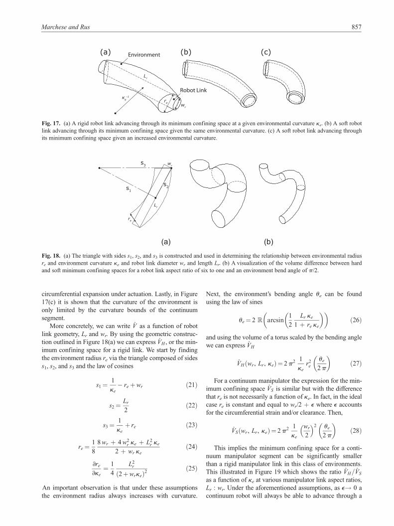
robot can pass and Figure 17 illustrates this concept. We

assume a rigid robot link is cylindrical with diameter wr

and length Lr. Figure 17(a) depicts a rigid link advancing

through the link’s minimum confining space, parameterized

by the environment’s radius re and its curvature ke. The

minimum confining space is dependent on both the link’s

geometry and the environment’s curvature. A segment of a

continuum manipulator with the same initial cylindrical

dimensions as the rigid link is advanced through the seg-

ment’s minimum confining space given the same environ-

mental curvature in Figure 17(b). Noticeably, the robot and

environment radius only differ by e to account for

Algorithm 2. Configuration controller.

Input: k0, kf, _kmax . 0, €kmax . 0, gResult: Manipulator moves along configuration trajectory from k0 to kf.

1 _k(t) generateTraj k0, kf , _kmax, €kmax� �

2 driveSegments _k(t), gð ÞProcedure generateTraj(k0, kf, _kmax, €kmax)

Result: _k(t) that takes segments from k0 at t = t0 to kf at t = tffor n = 1.N. do

All k in this loop are indexed by i but omitted for convenience

if kf � k0

\ 2_kmaxð Þ2€kmax then

_kmax SGN kf � k0

� � ffiffiffiffiffiffiffiffiffiffiffiffiffiffiffiffiffiffiffiffiffiffiffiffiffiffiffiffikf � k0

€kmax

q.

t1 kf�k0j j_kmaxj j .

t2 t1.

else

_kmax SGN kf � k0

� �_kmax.

t1 _kmaxj j€kmax .

t2 kf�k0j j_kmaxj j .

endtf t1 + t2.

t [0, t1, t2, tf, tf + e].

v 0, _kmax, _kmax, 0, 0½ �._k(t) firstOrderHold t, vð Þ.

endreturn _k(t)Procedure driveSegments( _k(t), g)

Result: Drive segments to desired configurationt t0.while t \ max(tf) do

if A new sensor measurement Ebaseis available then

Egn ½Tbase

g (g)��1Ebase

n 8 n = 1 N .

kmeas singleSegInvKin(Eg) (Marchese et al., 2014b).

ktarget R t

t0_kn(t) dt 8 n.

Send error (ktarget 2 kmeas) to low level cascaded PI-PID controllers (Marchese et al., 2014b).endt elapsed time.

endreturn


circumferential expansion under actuation. Lastly, in Figure

17(c) it is shown that the curvature of the environment is

only limited by the curvature bounds of the continuum

segment.

More concretely, we can write V as a function of robot

link geometry, Lr and wr. By using the geometric construc-

tion outlined in Figure 18(a) we can express VH , or the min-

imum confining space for a rigid link. We start by finding

the environment radius re via the triangle composed of sides

s1, s2, and s3 and the law of cosines

s1 =1

ke

� re + wr ð21Þ

s2 =Lr

2ð22Þ

s3 =1

ke

+ re ð23Þ

re =1

8

8 wr + 4 w2r ke + L2

r ke

2 + wr ke

ð24Þ

∂re

∂ke

=1

4

L2r

2 + wrkeð Þ2ð25Þ

An important observation is that under these assumptions

the environment radius always increases with curvature.

Next, the environment’s bending angle ue can be found

using the law of sines

ue = 2 R arcsin1

2

Lr ke

1 + re ke

� �� ð26Þ

and using the volume of a torus scaled by the bending angle

we can express VH

VH wr, Lr, keð Þ= 2 p2 1

ke

r2e

ue

2 p

� �ð27Þ

For a continuum manipulator the expression for the min-

imum confining space VS is similar but with the difference

that re is not necessarily a function of ke. In fact, in the ideal

case re is constant and equal to wr/2 + e where e accounts

for the circumferential strain and/or clearance. Then,

VS wr, Lr, keð Þ= 2 p2 1

ke

wr

2

� �2 ue

2 p

� �ð28Þ

This implies the minimum confining space for a conti-

nuum manipulator segment can be significantly smaller

than a rigid manipulator link in this class of environments.

This illustrated in Figure 19 which shows the ratio VH=VS

as a function of ke at various manipulator link aspect ratios,

Lr : wr. Under the aforementioned assumptions, as e! 0 a

continuum robot will always be able to advance through a

wr

Lr

reĸe-1

(a) (b) (c)Environment

Robot Link

Fig. 17. (a) A rigid robot link advancing through its minimum confining space at a given environmental curvature ke. (b) A soft robot

link advancing through its minimum confining space given the same environmental curvature. (c) A soft robot link advancing through

its minimum confining space given an increased environmental curvature.

s1

s2

s3 wr

re

Lr

(a) (b)

Fig. 18. (a) The triangle with sides s1, s2, and s3 is constructed and used in determining the relationship between environmental radius

re and environment curvature ke and robot link diameter wr and length Lr. (b) A visualization of the volume difference between hard

and soft minimum confining spaces for a robot link aspect ratio of six to one and an environment bend angle of p/2.


smaller confining environment than a rigid linked robot

when ke . 0. This volume difference increases with aspect

ratio and environmental curvature. Figure 18(b) visualizes

an example of this volume difference for a robot link aspect

ratio of six to one and an environment bend angle of p/2.

6.1.1. Confined environment evaluations. For an entirely

soft robot, where continuum kinematics and high compli-

ance are combined, this result implies that such a manipula-

tor can passively conform to the aforementioned class of

confined environments. When the portion of the arm within

the confined environment is passive e! 0 and when the

environment is composed of PCC cylinders, the above

assumptions are met. In order to experimentally validate

the soft fluidic elastomer manipulator’s ability to advance

through a confined environment we autonomously advance

a passive manipulator with an actuated base through a pipe.

Then, we actively perform a task once the manipulator is

fully inserted. The experiment is shown in Figure 20 as

well as Extension 1. The goal of the experiment is to repea-

tably advance the soft arm (Figure 20b) through a tightly

bending pipe (Figure 20(d)) using only a constant linear

and rotational motion of the manipulator’s base. This inser-

tion motion is provided by a motorized rotary and linear

stage (Figure 20(h) and (i), respectively). A camera located

at the arm’s end effector (Figure 20(c)) can be used to loca-

lize the pipe entrance, inspect the pipe, and view objects of

interest (Figure 20(f)) once the arm has exited the pipe.

Video from this end effector camera is shown in the supple-

mentary video submission. Because the arm’s fluidic trans-

mission system can deliver power independent of the arm’s

configuration, a tether (Figure 20(e)) allows the user to

actuate the most distal segment while the proximal portion

of the arm has passively conformed to the pipe environ-

ment, as is shown in Extension 1.

10 consecutive trials of the confined environment

experiment were performed, and the manipulator success-

fully advanced through the pipe in every trial and was able

to perform an actuated task after insertion every trial. The

confined environment consists of three 5 cm insider dia-

meter bent pipe segments each with a curvature of approxi-

mately 15.2 m21, motivated by the fact that the

manipulator’s maximum outside diameter is five centi-

meters with a two degree taper from tip to base. In all tests

the manipulator’s base was moved at a constant linear velo-

city and rotational velocity of 12 mm/s and 0.11 rev/s,

respectively. The base was moved until a fixed insertion

depth of 40 cm was reached. A thin layer of Talc powder

was applied to the surface of the silicone arm to reduce the

coefficient of friction between the robot’s surface and plas-

tic pipe. A load cell (Figure 20(g)) was used to measure

insertion force as a function of time. Figure 21 shows this

required resulting insertion force and insertion depth as a

function of time for all ten trials as well as the applied base

linear and rotational velocities as a function of time.

Across the ten trials the mean peak insertion force was

11.8 6 1.2 N.

It should be noted that we did not investigate pipe inser-

tions where the gross motion of the robot is orthogonal or

even opposite to gravity. We imagine that our current

approach to passive insertion may not be well-suited for

either of these scenarios. By employing a retractable sheath

extending to the tip of the manipulator (as opposed to the

static, base-segment sheath employed in the current experi-

ments) it is conceivable that the uninserted portion of the

manipulator could be sufficiently supported, potentially

allowing for such insertion scenarios.

6.2. Shape fitting

The continuum kinematics of a soft robot manipulator

enable a high degree of dexterity. Specifically, in an envi-

ronment where a collision-free path is parameterized by a

curved shape, a continuum manipulator can generally fit

the curvature of the path better than a rigid link manipula-

tor with discrete joints. Consider a path in planar cartesian

coordinates P(x(t), y(t)) parameterized by time t or equiva-

lently arc length s. The curvature at t can be expressed as

kp(t)=∂x

∂t

∂2y

∂t2� ∂y

∂t

∂2x

∂t2

� �=

∂x

∂t

2

+∂y

∂t

2� �3=2

ð29Þ

Because the first order Taylor series expansion

TS1(kp(t)) at t is constant, a soft continuum robot has the

capacity to locally approximate the path’s curvature to the

first order by adjusting the curvature of its neutral axis over

a continuum. In the case of no external forces, each of the

soft continuum N segments can be fit to approximate the

local curvature of the path under actuation

0 0.05 0.1 0.15 0.2 0.25 0.3 0.35 0.4 0.45 0.50

1

2

3

4

5

6

7

8

9

10

Enviroment Curvature [κe]

VH / V

S

3:1

6:1

5:1

4:1

7:1

7:1 3:1

Fig. 19. The ratio of a hard to soft robot’s minimum confining

volume cVH =cVS as a function of the curvature of the surrounding

environment ke. The robot’s minimum confining volume is the

volume of the smallest curved environment through which a

given robot can pass. The ratio is expressed for various robot link

aspect ratios Lr : wr. Both the hard and soft links have the same

initial geometry.


ki =1

Li

Z Li2

�Li2

TS1 kp(s)� �

ds 8 i = 1, . . . ,N ð30Þ

where L is the soft segment length. There are several sce-

narios that cause an error between the continuum robot’s

curvature and the path’s curvature. These scenarios are

detailed in Figure 22. Figure 22(a) depicts a scenario where

the path P(s), shown by the dotted line, has locally constant

curvature on the interval s = [a, b]; however, the arm seg-

ment’s neutral axis of approximately equal length, shown as

the solid line, has a maximum curvature kmax less than

kp(s) and this produces an error in shape fitting. Figure

22(b) depicts a scenario where the path’s local curvature on

the interval s = [a, b] is non-constant and this also causes an

error in the goodness of fit between the path and arm seg-

ment of approximately equal length. Lastly, Figure 22(c)

illustrates the scenario where the arm segment length L is

greater than the total path length. Although a quality shape

fit may be possible, this results in positional error either

normal to the path (left) or tangent to the path (right).

Fig. 20. Pipe insertion experiment. The experimental setup consists of serval components: (a) plastic sheath, (b) soft manipulator

prototype of maximum outside diameter 5 cm, (c) end effector camera, (d) confining pipe of inside diameter 5 cm, (e) power tether, (f)

objects of interest, (g) load cell, (h) automated rotary stage, and (i) automated linear stage. (A) Depiction of the manipulator prior to

pipe insertion. Here, the distal most arm segment is actuated to simulate localization of the pipe entrance. (B) Depiction of the passive

arm being autonomously inserted through the pipe by means of actuation at its base. (C) Depiction of the manipulator fully advanced

through the pipe and performing the actuated task of inspecting flowers with its end effector camera.

0 5 10 15 20 25 30 350

5

10

15

20

Inse

rtion

For

ce [N

]

0 5 10 15 20 25 30 350

20

40

60

Inse

rtion

Dep

th [c

m]

0 5 10 15 20 25 30 350

5

10

15

20

Line

ar V

eloc

ity [m

m/s

ec]

0 5 10 15 20 25 30 350

0.1

0.2

Rot

atio

nal V

eloc

ity [r

ev/s

ec]

Time [sec]

Fig. 21. Results of pipe insertion experiment. At the top,

measured insertion force as well as insertion depth is reported for

all 10 experimental trials. Generally the insertion force increased

with the insertion depth. At the bottom, the commanded linear

and rotational velocity of the manipulator’s base are shown

during the insertion phase of the experiment. The insertion phase

has positional end criteria, that is linear velocity is constant at

12 mm/s until a fixed insertion depth of 40 cm is reached upon

which motion is stopped. Note that base rotation begins several

seconds after linear motion, approximately when the manipulator

enters the pipe, and base rotation has a fixed velocity of 0.11 rev/

s until 2.43 revolutions are reached.

(b) (c)(a)

a

b

a

b

a

b

P(s)

Fig. 22. Several common scenarios that cause an error between

a continuum robot’s curvature and a path’s curvature. (a) The

maximum curvature of the robot is less than the local curvature

of the path on the interval s = [a,b]. (b) The local curvature of the

path is non-constant and the robot’s deformation is parameterized

by PCC arcs. (c) Description of a scenario where the robot’s

segment length is greater than the total path length.


In the case of a rigid link manipulator with discrete

joints, curvature along the neutral axis is either 6N, as by

definition this structure is not a continuum. In this case the

best way to approximate the curvature of a path is to

increase the number of links and decrease the link length

relative to the path length.

6.2.1. Shape fitting algorithm. To incrementally advance a

soft continuum manipulator along a curved path we pro-

pose the path following strategy described in Algorithm 3.

The fundamental idea of this path following approach is

that each segment is sequentially advanced onto the path.

For each segment on the path, two points along the seg-

ment’s neutral axis, the mid and endpoint, are fit to the path

by choosing the segment’s curvature k to minimize the

Euclidean norm between the two points and their projec-

tion onto the path. By adding two points for each segment

advanced onto the path plus the origin pose constraint, this

approach effectively samples the path’s curvature kp(s) as

two points and an initial orientation uniquely define a con-

stant curvature arc. This approach assumes the manipulator

has the capacity to position and orient a point along its

neutral axis that is a distance s from the manipulator’s tip,

to the path’s origin.

forwardKin() or the forward kinematics procedure

(see Algorithm 4) for recursively determining a point on

the arm located a distance s on segment i given curvature

and length was developed in Marchese et al. (2014b).

6.2.2. Shape fitting simulations. To demonstrate the differ-

ence between fitting a soft continuum and rigid-linked

robot to a curved path, we perform several simulations of

advancing both a soft and rigid manipulator backbone

through a curved path. The results of the simulations are

shown in Figure 23. The first column describes a given col-

lision free path through an environment. Columns two

through four show the backbone of a soft robot (blue) and

hard robot (red) advancing along and conforming to the

path with different link lengths. Their neutral axis is over-

laid at every time step. Both the soft and hard manipulators

have the same link length, and this is varied from 25% of

the total path length in column two to 41% of path length

in column four. In general, as the ratio of link length to path

length increases the number of error scenarios outlined in

Figure 22 increases, and the quality of fit decreases;

However, in these examples the soft continuum robot

approximated the curved path better than the rigid link

robot in all cases.

6.2.3. Single segment tracking experiments. First, we seek

to experimentally evaluate the ability of the closed-loop

controller, developed in Section 5, to regulate the curvature

of an individual arm segment. These experiments differ

from those in Marchese et al. (2014b) in that they are per-

formed using the spatial manipulator described in Section

3 which is an entirely new hardware system and with a

hanging manipulator that is subject to gravitational loading

and not supported by a plane. Figure 24 details a series of

experiments where a sinusoidal reference curvature is

tracked by the controller. The left-hand and right-hand col-

umns represent reference waves with angular frequencies

of 0.16 and 0.63 rads/sec, respectively.

Experiment 1 details the performance of the controller

tracking a wave centered about zero curvature. Notably, the

system has difficulty tracking curvatures around zero. A

Algorithm 3. Path fitting algorithm (for forwardKin() see Algorithm 4).

for t = 0 : dt : tf do

1 s tDs

dt:

2 N, L Determine the number of segments N that can be projected onto P and their corresponding lengths L as a function ofs and L0.

3 k� mink

PNi = 1

forwardKin k, L, i, Lið Þ � PPi

j = 1

Lj

!+

PNi = 1

forwardKin k, L, i, Li

2

� �� P

Pi

j = 1

Lj � Li

2

!

subject to kmini � ki� kmax

i 8 i = 1 N :

8><>:9>=>;

4 Servo continuum segments to k*

end

Algorithm 4. Forward kinematics algorithm.

Procedure forwardKin (k, L, i, s)Input: k, L, i the segment of interest index, s thearc length along the indexed segmentif i = 0 then

ui(0) u0(0).xi(0) 0.yi(0) 0.

else[xi(0), yi(0), ui(0)] forwardKin (k, L, i 2 1,Li2 1).

endu ui(0) + kis.

x xi(0)+sin u

ki

� sin ui(0)

ki

.

y yi(0)�cos u

ki

+cos ui(0)

ki

.

return [x, y, u]Tor[x, y]T


likely explanation for this behavior is the severe nonlinear

deformation encountered when inflating a thin-walled tube

detailed in Gent (2012). In short, there can be two stable

configurations of the expanding tube for a given internal

pressure above a certain critical pressure. Evidence of this

behavior can be observed directly in Figure 10(b).

Although the actuated channel is uniformly pressurized, the

elastomer exhibits both aneurysm-like areas of large defor-

mation as well as areas of relatively small deformation. We

attribute the difficulty in regulating segment curvature

around zero to the nonlinear, bi-stable deformation charac-

teristics of this particular channel geometry.

During Experiment 2, the same reference trajectories

were tracked; however, the agonist and antagonist channels

were each pre-filled with 50 ccm of air prior to the start of

the experiment and automatic piston adjustments. Our

hypothesis is that by pre-pressurizing the channels, the crit-

ical inflation pressure can be achieved with smaller piston

motions and thus the large deformation configuration (the

deformation responsible for producing appreciable

curvature) is reached with less delay. Experimentally, we

observed improvements in tracking performance using this

method; however, these improvements were not consistent

throughout Experiment 2. For example, while tracking the

lower frequency wave the actuated channel responsible for

negative curvature performed almost identical between

Experiment 1 and 2, despite the added pre-pressurization.

Again, we attribute this to the fact that a large and small

deformation configuration are both viable and stable at

these inflation pressures. We observed performance

improvements while tracking the higher frequency wave

with the pre-pressurization approach.

Lastly, Experiment 3 shows the ability of the controller

to track the low and high frequency curvature trajectories

without pre-pressurization when the wave trajectory is

biased away from zero. In this experiment, the offset of the

sine wave begins at zero and is gradually increased to

7.5 m21 where it is held. As expected, initial tracking about

near-zero curvatures is difficult, but once the bias suffi-

ciently increases the tracking performance improves. The

Fig. 23. Shape fitting simulations. In the first column, a collision free curved path through several environments is given. In the

second, third, and fourth columns a soft robot with a PCC backbone (Webster and Jones, 2010), shown in blue, and a hard robot with

fixed joints, shown in red, are sequentially advanced along and fit to the path in the first column using Algorithm 3. Manipulator link

length is varied from 25% of total path length in column two to 41% of path length in column four as indicated by the ratios above

each column.


bias effectively serves to keep the inflation pressure above

the pressures resulting in the bi-stable channel

deformations.

6.2.4. Multi-segment tracking experiments. The purpose of

the experiments performed in this section is to evaluate the

aggregate soft manipulation system’s ability to autono-

mously control the configuration of the soft arm. That is,

in real-time with the closed-loop controller developed in

Section 5, we drive the arm’s measured curvature represen-

tation kmeasured to a desired reference shape parameterized

by ktarget. We demonstrate that the arm is able to conform

to a user specified configuration within a sagittal plane

index by g. To the best of our knowledge, this is the first

demonstration of closed-loop curvature control for a fluidic

elastomer robot not constrained to planar motion.

The goal of the experiments detailed in Figures 25 and

26 as well as in Extension 2 is for the soft manipulator to

autonomously transition from a neutral, hanging state (i.e.

u0 = 3p/2 and k0’0) to either an S shape (see Figure 25)

or a C shape (see Figure 26). Ten and twelve trials of the S

and C shape experiments were performed, respectively, and

the results for all trials are shown in Figures 25 and 26,

respectively. In the S-shaped configuration experiment,

segments were less prone to twisting about their neutral

axis (an unactuated DOF), and accordingly it was sufficient

to use a single pair of agonist actuators collocated with the

sagittal plane to achieve the required bending (schemati-

cally represented Figure 5C(d)). However, during the C-

shaped configuration experiment, segments were more

prone to twisting about their neutral axis. To counter this

phenomenon, two pairs of agonist actuators were collo-

cated with the sagittal plane, i.e. each pair was offset 45�from the sagittal plane (schematically represented Figure

5C(c)). This actuation strategy provides equal and opposite

components of force that stabilize the segment’s bending

along the sagittal plane.

Experiment1

0 2 4 6 8 10−6

−4

−2

0

2

4

6

Time [sec]

Cur

vatu

re [1

/m]

MeasuredReference

0 2 4 6 8 10−6

−4

−2

0

2

4

6

Time [sec]

Cur

vatu

re [1

/m]

Experiment2

0 2 4 6 8 10−6

−4

−2

0

2

4

6

Time [sec]

Cur

vatu

re [1

/m]

0 2 4 6 8 10−6

−4

−2

0

2

4

6

Time [sec]

Cur

vatu

re [1

/m]

Experiment3

0 5 10 15−14

−12

−10

−8

−6

−4

−2

0

Time [sec]

Cur

vatu

re [1

/m]

0 5 10 15−20

−15

−10

−5

0

5

Time [sec]

Cur

vatu

re [1

/m]

Fig. 24. A series of experiments characterizing the performance of the control system to track sine wave reference trajectories. In

Experiment 1 the wave offset is zero, in Experiment 2 the wave offset is again zero but the channels are pre-pressurized, and lastly

during Experiment 3 the offset is gradually increased away from zero to a fixed 7.5 m21 and no pre-pressurization is used.


Panel (a) in Figures 25 and 26 depicts the reference cur-

vature trajectory, ktarget(t), in red and measured curvature

trajectory, kmeasured, in black as a function of time, as deter-

mined by Algorithm 2 developed in Section 5. Note that,

three out of the four segments are actively controlled, and

the base segment is left passive in order to dampen oscilla-

tions arising from distal segment movement. Panel (b)

shows the reference (red) and measured (black) manipulator

configuration at t = 20. Panel (c) contains photographs of the

soft fluidic elastomer arm prototype during the experiments.

The mean one standard deviation steady state curvature

errors across all the trials for the C shape were 0.05 6 0.09,

20.04 6 0.07, and 0.02 6 0.09 m21, respectively for seg-

ments two through four respectively. The steady state curva-

ture errors across all the trials for the S shape were 20.11 6

0.03, 20.02 6 0.07, and 0.03 6 0.12 m21, respectively.

0 5 10 15 20−15

−10

−5

0

5

10

15

20

25

Time [sec]

Cur

vatu

re [1

/m]

(a)

−0.1 0 0.1−0.5

−0.4

−0.3

−0.2

−0.1

0

0.1

x [m]

z [m

]

(b) (c)

Fig. 25. Experimental evaluations of closed-loop real-time configuration control. In 10 consecutive trials, the aggregate manipulation

system is provided an S shaped goal configuration to reach, shown in red in (b). The goal configuration state is parameterized by three

target curvatures kf = [5, 210, 20] for segments two to four respectively. Algorithm 2 plans a reference configuration trajectory k(t),

shown in red in (a), and drives the arm along this configuration trajectory by measuring the arm’s current configuration, shown in

black in (a), and adjusting the volumetric displacement of the fluidic drive cylinder array. (c) The prototype fluidic elastomer

manipulator in the target configuration.

0 5 10 15 20−10

−5

0

5

10

15

20

25

Time [sec]

Cur

vatu

re [1

/m]

(a)

−0.1 0 0.1−0.5

−0.4

−0.3

−0.2

−0.1

0

0.1

x [m]

z [m

]

(b) (c) (d)

Fig. 26. Experimental evaluations of closed-loop real-time configuration control. In 10 consecutive trials, the aggregate manipulation

system is provided a C shaped goal configuration to reach, shown in red in (b). The goal configuration state is parameterized by three

target curvatures and 10 trials used the goal kf = [25, 5, 20] and two trials used the goal kf = [25, 10, 20] for segments two to four

respectively. Algorithm 2 plans a reference configuration trajectory k(t), shown in red in (a), and drives the arm along this

configuration trajectory by measuring the arm’s current configuration, shown in black in (a), and adjusting the volumetric

displacement of the fluidic drive cylinder array. (c, d) The prototype fluidic elastomer manipulator in the target configurations. (d)

Reproduced with kind permission from Mary Ann Liebert Inc. (Marchese et al., 2015a)


6.3. Positioning

Additionally the soft arm is capable of Cartesian position-

ing in three dimensions. Similar to the approach in

Marchese et al. (2014a), we pose the inverse kinematics

problem (i.e., the transformation from the manipulator’s

task space to its arc space) as a constrained nonlinear opti-

mization, allowing phenomena arising from the arm’s soft-

ness to be expressed as numerical constraints. More

specifically, we can calculate g as well as find a locally-

optimal reference configuration k* that position the arm’s

end-effector at a goal point within a statically reachable

envelope. For more information on finding points within a

statically reachable envelope please refer to Marchese et al.

(2015b). Once a suitable reference configuration is deter-

mined, we can again use the procedures outline in

Algorithm 2 to both plan an execute a curvature trajectory

trajectory _k(t).

6.3.1. Positioning algorithm. First, the procedure

moveToObject in Algorithm 5 localizes an object’s cen-

ter in R3 using the external camera system, a process rep-

resented by localizeObject(). To obtain a target

end-effector position, the object’s position is translated a

predetermined offset based on the object’s geometry using

the transformation Tobjectoffset .

The strategy for moving the arm to this goal point is

represented in the procedure moveToPoint(). First, the

arm is rotated into a sagittal plane defined by the angle g

by means of the base rotary stage. The vertical plane is

coincident with both the base frame’s origin and the goal

point. The end-effector is then iteratively moved in this

plane towards the goal point by finding locally-optimal ref-

erence configurations. This iterative search for manipulator

configurations starts, as previously mentioned, by taking a

set of real-time endpoint measurements Ebasen , projecting

them into the sagittal plane using the simple transformation

Algorithm 5. Algorithm for three-dimensional positioning.

Procedure moveToObject()

[xobject, yobject, zobject] localizeObject().

xoffset, yoffset, zoffset½ �T Tobjectoffset xobject, yobject, zobject

� �T. moveToPoint (xobject, yobject, zobject).

returnProcedure moveToPoint(xbase, ybase, zbase)

g arctan ybase

xbase

� �.

xg, yg, zg½ �T ½Tbaseg (g)��1

xbase, ybase, zbase� �T

.

Move rotary stage to g.

while forwardKin kmeas, Lmeas, N , LmeasNð Þ � xg

zg

� e do

Wait until a new sensor measurement Ebase is available.

Egn ½Tbase

g (g)��1Ebase

n 8 n = 1 . . . N

kmeas, Lmeas singleSegInvKin(Eg) (Marchese et al., 2014b)

kf inverseKin xg, zg, kmeas1ð Þ

_k(t) generateTraj kmeas, kf , _kmax, €kmax� �

driveSegments _k(t), gð Þ;end

returnProcedure inverseKin x, y, kmeas1

ð Þ

R a weighting vector,

umin and umax constraints on end-effector approach angle.

k� mink

PNi = 1

Ri ki

subject to f forwardKin k, Lmeas, N , LmeasNð Þ

x

y

�� f1

f2

�= 0

kmeas1� k1 = 0

umin � f3 � umax

kminn �kn�kmax

n 8 n = 1, . . . ,Nreturn k*


Tbaseg (g) to arrive at the set Eg

n . This data is passed to the

procedure singleSegInvKin() in order to uniquely fit

a PCC model to the data, providing a measured manipula-

tor configuration representation kmeas. This provides the

current manipulator configuration from which the trajec-

tory _k(t) is started. To determine the trajectory’s end con-

figuration kf, the optimization-base inverse kinematics

procedure, represented by inverseKin(), is invoked.

This process finds a weighted minimal-strain solution sub-

ject to:

(a) the end-effector being positioned at the goal point

projected into the sagittal plane;

(b) the state of the passive base segment, kmeas1, appro-

priately limiting the configuration’s DOF;

(c) end-effector orientation being constrained, in combi-

nation with curvature limitations, in order to prevent

configurations where the center of mass of segment n

is above connector piece n 2 1 for static stability pur-

poses; and

(d) empirically determined curvature limits not being

exceeded.

After defining kmeas and kf the previously defined pro-

cedure generateTraj() is used to generate a realizable

configuration trajectory and the procedure

driveSegments() is used to move the manipulator

along this trajectory. The process is repeated until the end-

effector is within e of the goal location.

6.3.2. Positioning evaluations. In order to experimentally

evaluate the three-dimensional positioning capabilities of

the soft arm we ran Algorithm 5 on the manipulation sys-

tem. The goal of the experiment was for the soft arm to

move its end-effector into contact with a 4 cm diameter

table tennis ball placed within the arm’s statically reachable

envelope. The purpose of the experiment was to evaluate

the arm’s positioning capabilities, not to robustly pick-up

the ball. Accordingly, velcro was simply fixed to both the

ball and end-effector to perform the pick-up.

In 10 consecutive attempts, the manipulation system

was able to successfully position the arm’s end effector to

make contact with the ball. The object offset translation

Tobjectoffset underwent minor adjustments throughout the tests

to continually improve the contact between the velcro

pieces. Figure 27(a)–(d) as well as Extension 3 detail one

of these trials. Figure 27(a) shows the first reference con-

figuration kf planned by Algorithm 5 in red as well as the

configuration representation kmeas fit to measured endpoint

data at tf in blue. The discrepancy between kf and kmeas is

almost imperceptible. At this point the end-effector and

object made contact (see 27(c)). Figure 27(b) shows the

second reference configuration planned by the algorithm,

considering the passive bending of the first segment, again

shown in red. Noticeably, the manipulator’s measured con-

figuration representation, again shown in blue, deviates sig-

nificantly from this plan as the manipulator’s end-effector

is already in contact with the object inhibiting the manipu-

lator’s motion in the desired direction. Lastly, Figure 27(d)

shows intermediate target curvatures ktarget (red) as well as

intermediate measured configuration representations kmeas

(black) from t0 to tf for each segment. The compressibility

of the transmission medium as well as the relatively large

residual volume of the pistons explain the several second

−0.2

0

0.2

−0.2 −0.1 0 0.1 0.2

−0.7

−0.6

−0.5

−0.4

−0.3

−0.2

−0.1

0

x [m]

y [m]

z [m

]

(a)

−0.2

0

0.2

−0.2 −0.1 0 0.1 0.2

−0.7

−0.6

−0.5

−0.4

−0.3

−0.2

−0.1

0

x [m]

y [m]

z [m

]

(b) (c)

8 10 12 14 16 18−15

−10

−5

0

5

10

15

Time [sec]

Cu

rva

ture

[1

/m]

(d)

Fig. 27. Experimental evaluations of three-dimensional end-effector positioning with the soft manipulator prototype. (a) Algorithm 5

plans a locally-optimal, minimal-strain reference configuration (red) to which the arm’s measured configuration representation is

driven (blue). Here, contact is made between the end-effector and object. (b) The algorithm’s next plan is shown that would

theoretically bring the manipulator’s end-effector even closer to the intended target but physical contact with the object prevents the

new target configuration from being reached. (c) A photograph of the manipulator’s end effector making contact with the object of

interest. (d) The first intermediate reference configuration trajectory ktarget(t) is shown in red and the measured configuration

representation of the manipulator is shown in black kmeas(t).


delay in tracking the reference configuration. We have

recently shown that by using techniques such a pre-

pressurization and tandem inflation this performance char-

acteristic can be improved (Katzschmann et al., 2015).

7. Conclusion

In this work we presented an autonomous fluidic elastomer

spatial manipulation system. We developed a new spatial

manipulator morphology that is modular in design and well

suited for automation. We constructed multiple physical

prototypes of this soft arm using an innovative multi-step

casting process that extends our approach to building

manipulators from two dimensions (Marchese et al.,

2014a) to three dimensions. We developed, simulateed, and

experimentally validated a static model in order to under-

stand how a single segment of this manipulator deforms.

Then, using a piece-wise constant curvature assumption

(Webster and Jones, 2010), we modeled the multi-segment

kinematics of the soft manipulator. To power the manipula-

tor, we developed an array of high capacity fluidic drive

cylinders, again extending our approach to powering planar

manipulation (Marchese et al., 2014b) into three dimen-

sions. To control the arm in a rotating sagittal plane we

developed a real-time closed-loop control algorithm that

generates realizable curvature trajectories, measures the

arms current state using localized segment endpoints, and

leverages a cascaded control strategy we developed for our

planar systems. These innovations in actuation, modeling,

fabrication, power, and processing and control enable new

manipulation capabilities for soft robots. We demonstrate

the arm’s ability to enter and advance through a confined

spatial environment. We demonstrate that the soft manipu-

lator prototype can use its passive compliance and softness

to repeatedly advance through and conform to a complex

pipe shape. In addition, because of its configuration-

independent fluidic power transmission, the manipulator

can perform actuated tasks with its distal most segments,

once they have advanced through the confining environ-

ment. Another new capability is the aggregate soft manipu-

lation system’s ability to autonomously control the

configuration of the soft arm. That is, in real-time with a

closed-loop controller we show that a user-specified goal

configuration can be repeatedly achieved with minimal

shape error.

7.1. Limitations

There are several notable limitations within the presented

work. In general, the presented actuator design does not

explicitly consider the rupturing or failure of the elastic

material. Although we have found the chosen physical

dimensions of the soft elastomer actuators suitable for the

number and type of experiments presented here, these are

certainly not optimal and we also do not provide an

investigation into the onset of plastic deformation or

dynamic material fatigue. This is certainly a concern when

actuator motions are fast, repetitive, and of relatively large

magnitude. Furthermore, due to the nonlinear deformation

profile of the presented channel geometry, the onset of

these adverse phenomena may not be easy to predict.

Future work is needed to investigate the dynamic beha-

vior of such elastomer-based robots. This study is limited to

purely kinematic modeling and motion control. We have

found this approach viable for controlling the configuration

of the robot within a limited, statically reachable envelop;

however, it is important to note that this reachable envelope

is significantly constrained due to the force-limits of the pro-

posed actuators and the need to compensate for the weight

of multiple, distally suspended segments.

In addition, the developed soft manipulator has many

passive DOFs and these can contribute to various

motions both desirable and undesirable. For example,

using the manipulator’s passive DOFs we are able to

achieve pipe insertion as detailed in Section 6.1; how-

ever, during configuration tracking experiments, passive

DOFs lead to significant oscillations in the system’s

motion in the presence of external disturbances (please

refer to Extension 1). In future work, a proper character-

ization of these passive DOFs could lead to model-

based controllers that are capable of removing or even

leveraging these phenomena.

Acknowledgements

We would like to thank Robert Katzschmann for his continual help

in brainstorming and troubleshooting as well as for his review of

this paper, Jose Lara and Jonathan Lambert for their assistance in

fabricating duplicate prototypes and for their help evaluating alter-

native designs, and to Ross Knepper for brainstorming soft arm

capabilities.

Funding

This work was supported by the National Science Foundation,

(grant numbers NSF 1117178, NSF IIS1226883, and NSF

CCF1138967) and by the NSF Graduate Research Fellowship

Program, (grant number 1122374).

References

Buckingham R (2002) Snake arm robots. Industrial Robot: An

International Journal 29(3): 242–245.

Calisti M, Arienti A, Giannaccini ME, et al. (2010) Study and

fabrication of bioinspired octopus arm mockups tested on a

multipurpose platform. In: 2010 3rd IEEE RAS and EMBS

international conference on biomedical robotics and biome-

chatronics (BioRob), Tokyo, Japan, 26–29 September 2010,

pp. 461–466. Piscataway: IEEE.

Calisti M, Giorelli M, Levy G, et al. (2011) An octopus-

bioinspired solution to movement and manipulation for soft

robots. Bioinspiration and Biomimetics 6(3): 036002.


Camarillo DB, Carlson CR and Salisbury JK (2009) Configura-

tion tracking for continuum manipulators with coupled tendon

drive. IEEE Transactions on Robotics 25(4): 798–808.

Chen G, Pham MT and Redarce T (2006) Development and kine-

matic analysis of a silicone-rubber bending tip for colonoscopy.

In: 2006 IEEE/RSJ international conference on intelligent

robots and systems, Beijing, 9–15 October 2006, pp. 168–173.

Piscataway: IEEE.

Chirikjian GS and Burdick JW (1994) A hyper-redundant manipu-

lator. IEEE Robotics and Automation Magazine 1(4): 22–29.

Cieslak R and Morecki A (1999) Elephant trunk type elastic

manipulator-a tool for bulk and liquid materials transportation.

Robotica 17(1): 11–16.

Correll N, Onal CD, Liang H, et al. (2014) Soft autonomous

materials - using active elasticity and embedded distributed

computation. In: Khatib O, Kumar V and Sukhatme G (eds)

Experimental Robotics: The 12th International Symposium on

Experimental Robotics. Berlin: Springer, 227–240.

Deimel R and Brock O (2013) A compliant hand based on a novel

pneumatic actuator. In: 2013 IEEE international conference on

robotics and automation, Karlsruhe, Germany, 6–10 May

2013, pp. 2047–2053. Piscataway: IEEE.

Deimel R and Brock O (2014) A novel type of compliant, under-

actuated robotic hand for dexterous grasping. In: Proceedings

of robotics: science and systems, 1687–1692. Available at:

http://www.roboticsproceedings.org/rss10/p18.html (accessed

14 August 2015).

Gent AN (2012) Engineering with Rubber: How to Design Rubber

Components. Munich: Carl Hanser Verlag GmbH Co. KG.

Giorelli M, Renda F, Calisti M, et al. (2012) A two-dimensional

inverse kinetics model of a cable driven manipulator inspired

by the octopus arm. In: 2012 IEEE International conference on

robotics and automation, Saint Paul, USA, 14–18 May 2012,


Gravagne IA, Rahn CD and Walker ID (2003) Large deflection

dynamics and control for planar continuum robots. IEEE/

ASME Transactions on Mechatronics 8(2): 299–307.

Gravagne IA and Walker ID (2002) Uniform regulation of a multi-

section continuum manipulator. In: Proccedings of the ICRA

2002 IEEE international conference on robotics and automa-

tion, vol. 2, Washington, DC, USA, 11–15 May 2002, pp.

1519–1524. Piscataway: IEEE.

Hannan MW and Walker ID (2003) Kinematics and the implemen-

tation of an elephant’s trunk manipulator and other continuum

style robots. Journal of Robotic Systems 20(2): 45–63.

Jones BA and Walker ID (2006a) Kinematics for multisection con-

tinuum robots. IEEE Transactions on Robotics 22(1): 43–55.

Jones BA and Walker ID (2006b) Practical kinematics for real-

time implementation of continuum robots. IEEE Transactions

on Robotics 22(6): 1087–1099.

Kang R, Branson DT, Zheng T, et al. (2013) Design, modeling

and control of a pneumatically actuated manipulator inspired

by biological continuum structures. Bioinspiration and Biomi-

metics 8(3): 036008.

Katzschmann RK, Marchese AD and Rus D (2014) Hydraulic

autonomous soft robotic fish for 3d swimming. In: Interna-

tional symposium on experimental robotics (ISER), Marrakech

and Essaouira, Morocco, 15–18 June 2014 (in press).

Katzschmann RK, Marchese AD and Rus D (2015) Autonomous

object manipulation using a soft planar grasping manipulator

(in press).

Laschi C, Cianchetti M, Mazzolai B, et al. (2012) Soft robot arm

inspired by the octopus. Advanced Robotics 26(7): 709–727.

McEvoy MA and Correll N (2014) Shape change through pro-

grammable stiffness. In: International symposium on experi-

mental robotics, Marrakech and Essaouira, Morocco, 15–18

June 2014 (in press).

McMahan W, Chitrakaran V, Csencsits M, et al. (2006) Field

trials and testing of the octarm continuum manipulator. In:

Proceedings 2006 of the IEEE international conference on

robotics and automation, Orlando, USA, 15–19 May 2006,


McMahan W, Jones BA and Walker ID (2005) Design and imple-

mentation of a multi-section continuum robot: Air-octor. In:

2005 IEEE/RSJ international conference on intelligent robots

and systems, Edmonton, Canada, 2–6 August 2005, pp. 2578–

2585. Piscataway: IEEE.

Mahl T, Mayer AE, Hildebrandt A, et al. (2013) A variable curva-

ture modeling approach for kinematic control of continuum

manipulators. In: 2013 american control conference, Washington,

DC, USA, 17–19 June 2013, pp. 4945–4950. Piscataway: IEEE.

Marchese AD, Katzschmann RK and Rus D (2014a) Whole arm

planning for a soft and highly compliant 2D robotic manipula-

tor. In: 2014 IEEE/RSJ international conference on intelligent

robots and systems, Chicago, USA, 14–18 September 2014,


Marchese AD, Komorowski K, Onal CD, et al. (2014b) Design

and control of a soft and continuously deformable 2D robotic

manipulation system. In: 2014 IEEE international conference

on robotics and automation, Hong Kong, China, 31 May–7

June 2014, pp. 2189–2196. Piscataway: IEEE.

Marchese AD, Katzschmann RK and Rus D (2015a) A recipe for

soft fluidic elastomer robots. Soft Robotics 2(1): 7–25.

Marchese AD, Onal CD and Rus D (2011) Soft robot actuators

using energy-efficient valves controlled by electropermanent

magnets. In: 2011 IEEE/RSJ international conference on intel-

ligent robots and systems, San Francisco, USA, 25–30 Sep-

tember 2011, pp. 756–761. Piscataway: IEEE.

Marchese AD, Onal CD and Rus D (2014c) Autonomous soft

robotic fish capable of escape maneuvers using fluidic elasto-

mer actuators. Soft Robotics 1(1): 75–87.

Marchese AD, Tedrake R and Rus D (2015b) Dynamics and tra-

jectory optimization for a soft spatial fluidic elastomer manip-

ulator. In: 2015 IEEE international conference on robotics and

automation (ICRA), Seattle, USA, 26–30 May 2015, pp.

2528–2535. Piscataway: IEEE.

Martinez RV, Branch JL, Fish CR, et al. (2013) Robotic tentacles

with three-dimensional mobility based on flexible elastomers.

Advanced Materials 25(2): 205–212.

Miura K and Furuya H (1988) Adaptive structure concept for

future space applications. AIAA journal 26(8): 995–1002.

Miura K, Furuya H and Suzuki K (1985) Variable geometry truss

and its application to deployable truss and space crane arm.

Acta Astronautica 12(7): 599–607.

Onal CD and Rus D (2013) Autonomous undulatory serpentine

locomotion utilizing body dynamics of a fluidic soft robot.

Bioinspiration and Biomimetics 8(2): 026003.

Onal CD, Chen X, Whitesides GM, et al. (2011) Soft mobile

robots with on-board chemical pressure generation. In: Inter-

national symposium on robotics research, Flagstaff, USA, 28

August–1 September 2011. Available at: http://www.isrr-

2011.org/ISRR-2011/Program_files/Papers/Onal-ISRR-2011.

pdf (accessed 14 August 2015).


Pritts MB and Rahn CD (2004) Design of an artificial muscle con-

tinuum robot. In: Proceedings of the ICRA 2004 IEEE interna-

tional conference on robotics and automation, vol. 5, New

Orleans, USA, 26 April–1 May 2004, pp. 4742–4746. Piscat-

away: IEEE.

Robinson G and Davies JBC (1999) Continuum robots-a state of

the art. In: Proceedings of the 1999 IEEE international confer-

ence on robotics and automation, vol. 4, Detroit, USA, 10–15

May 1999, pp. 2849–2854. Piscataway: IEEE.

Sanan S, Moidel J and Atkeson C (2011) A continuum approach

to safe robots for physical human interaction. In: International

symposium on quality of life technology (isQoLT), Toronto,

Canada, 6–7 June 2011.

Shepherd RF, Ilievski F, Choi W, et al. (2011) Multigait soft robot.

Proceedings of the National Academy of Sciences 108(51):

20400–20403.

Shepherd RF, Stokes AA, Freake J, et al. (2013) Using explosions

to power a soft robot. Angewandte Chemie 125(10):

2964–2968.

Suzumori K, Iikura S and Tanaka H (1991) Development of flex-

ible microactuator and its applications to robotic mechanisms.

In: Proceedings of the IEEE international conference on

robotics and automation, Sacramento, USA, 9–11 April 1991,


Tolley MT, Shepherd RF, Mosadegh B, et al. (2014) A resilient,

untethered soft robot. Soft Robotics 1(3): 213–223.

Trimmer BA, Takesian AE, Sweet BM, et al. (2006) Caterpillar

locomotion: A new model for soft-bodied climbing and bur-

rowing robots. In: 7th international symposium on technology

and the mine problem vol. 1 Monteray, USA, 2–4 May 2006,

pp. 1–10. Monterey: Mine Warfare Association.

Trivedi D, Rahn CD, Kier WM, et al. (2008) Soft robotics: Biolo-

gical inspiration, state of the art, and future research. Applied

Bionics and Biomechanics 5(3): 99–117.

Umedachi T, Vikas V and Trimmer B (2013) Highly deformable

3D printed soft robot generating inching and crawling locomo-

tions with variable friction legs. In: 2013 IEEE/RSJ interna-

tional conference on intelligent robots and systems (IROS),

Tokyo, Japan, 3–7 November, pp. 4590–4595. Piscataway:

IEEE.

Wang H, Chen W, Yu X, et al. (2013) Visual servo control of

cable-driven soft robotic manipulator. In: 2013 IEEE/RSJ inter-

national conference on intelligent robots and systems (IROS),

Tokyo, Japan, 3–7 November 2013, pp. 57–62. Piscataway:

IEEE.

Webster RJ and Jones BA (2010) Design and kinematic modeling

of constant curvature continuum robots: A review. The Interna-

tional Journal of Robotics Research 29(13): 1661–1683.

Webster RJ, Romano JM and Cowan NJ (2009) Mechanics of

precurved-tube continuum robots. IEEE Transactions on

Robotics 25(1): 67–78.

Appendix A: Index to Multimedia Extensions

Archives of IJRR multimedia extensions published prior to

2014 can be found at http://www.ijrr.org, after 2014 all

videos are available on the IJRR YouTube channel at http://

www.youtube.com/user/ijrrmultimedia

Appendix B: Notation

Rx, Ry, Rz Rotation matrices about the subscript

Cartesian axis in R3

Tx, Ty, Tz Translation matrices along the

subscript Cartesian axis in R3

T Transformation matrix in R3bi, bj, bk Unit vectors codirectional with the

Cartesian coordinate system

k, u, L Curvature, bend angle, and

undeformed length of a soft arm

segment’s actuated region, respectively

k0, kf,

kmeas, ktarget

Initial, final, measured representation,

and target manipulator configuration

vectors, respectfully

k(t), _k(t),€k(t),

Curvature, velocity, and acceleration

configuration trajectories, respectfully

N Total number of segments in a multi-

segment manipulator

Ebasen , Eg

n A set of measured segment endpoint

data in the base frame (i.e. � R3) and

projected into the sagittal plane defined

by g (i.e. � R2), respectfully. The

segment number is indexed by n = 1,

., N

uP, LP Bend angle and undeformed length of

a soft arm segment’s unactuated region,

respectively

g Orientation of bend angle u

s Arc length

Table of Multimedia Extensions

Extension Mediatype

Description

1 Video A video of an exemplary experimentalevaluation from Section 6.1. This videodemonstrates the soft fluidic elastomermanipulator’s ability to advancethrough a tightly bending pipe usingonly the constant linear and rotationalmotion of the manipulator’s base.

2 Video A video of exemplary experimentalevaluations from Section 6.2. Here, thesoft manipulator autonomouslytransitions from a neutral, hanging state(i.e. u0 = 3p/2 and k0’0) to either an Sshape (see Figure 25) or a C shape (seeFigure 26) under closed-loopconfiguration control.

3 Video A video of exemplary experimentalevaluations from Section 6.3. Thisvideo shows an experiment where thesoft arm moves its end-effector intocontact with a 4 cm diameter tabletennis ball placed within the arm’sstatically reachable envelope.


pc Channel fluid pressure

sc, ec Circumferential material stress and

strain, respectively

sL, eL Longitudinal material stress and strain,

respectively�h, �w, �t, �u Channel diameter, wall length, wall

thickness, and bend angle of a thin

cross-sectional slice of a soft actuator,

respectively

h, w, t Deformed channel dimensions�A Cross-section area of a slice

J Total number of x–y cross-sectional

slices of a segment’s actuated region

uP, uM Model predicted bending angle and

measured bending angle, respectively

GP, GM Model predicted center of gravity and

measured center of gravity. respectively

V Minimum confining spaces, or the

smallest curved environment through

which a given robot link can pass

VH , VS Minimum confining space for a hard

and entirely soft link, respectively

wr, Lr, Diameter and length of a cylindrical

robot link

re, ke, ue Environment radius, curvature, and

bend angle, respectively

P A path in planar cartesian coordinates

kp Path curvature

TS1 First order Taylor series expansion

t Time

tf Final time

dt Discrete time interval


Date post:	26-May-2020
Category:	Documents
Upload:	others
View:	11 times
Download:	0 times

Design, kinematics, and control of a soft - MIT...

Documents