Design of an Eddy Current Probe for Cancer Detection

Undergraduate Thesis

Presented in Partial Fulfillment of the Requirements for Undergraduate Research in the

College of Engineering of The Ohio State University

By

Scott Koch

Department of Mechanical and Aerospace Engineering

The Ohio State University

2014

Defense Committee:

Prof. Vish Subramaniam, Advisor

Prof. Shaurya Prakash

________________________________

Approved: Prof. Vish Subramaniam

brought to you by COREView metadata, citation and similar papers at core.ac.uk

provided by KnowledgeBank at OSU

Copyright by

Scott Richard Koch

2014

ii

Abstract

Surgery is the main treatment option for solid tumors. Surgeons use palpation and

sight to identify and remove these malignant tumors during surgery. Surgically excised

tissue are marked only at a few locations for pathological analysis so that much less than

1% of the excised tissue is actually analyzed. Analysis of all removed tissue could enable

surgeons to decide in real-time whether or not more surgical intervention is necessary.

The overall goals of this research are (1) to develop a tool that surgeons can use to

quantify the boundaries of tumors embedded in excised tissue, and (2) to provide an

objective basis for determining in real-time whether or not any additional surgical

intervention is necessary while the patient is still in the operating room (OR). Recent

work at OSU has shown that eddy currents induced in tissue by a time-varying magnetic

field can be used to distinguish between cancer-bearing and normal tissue. The objectives

of this project are to design, construct, and optimize an eddy current detector for real-time

detection of malignant solid tumor boundaries. The eddy current probe comprises two

coaxial coils, the inner of which is the primary and the outer serves as the detector. Inter-

layer effects are explored by removing a detector coil layer from a previous probe design

and the effect of the probe’s intrinsic capacitance is explored by varying the insulation

iii

thickness of the probe wires. The probes are then characterized and evaluated using

measurements on animal tissue. It is found that removing a layer of windings in the

detector coil sharply reduces the detector coil’s inductance and voltage signal when

measuring tissue. Furthermore it is found that the intrinsic probe capacitance due to wire

insulation thickness also affects the detector signal, but to a lesser extent than removing a

detector coil layer. Both the number of detector coil layers and intrinsic probe

capacitance affect the ability of the eddy current probe to detect tissue and determine

contrast between tissue types.

iv

Dedication Dedicated to my family and friends

v

Acknowledgements

I would like to thank my advisor, Vish Subramaniam, for his extensive support and

guidance. I have learned so much from him over the course of this research.

I would like to thank Joe West for his ingenuity and assistance.

I would like to thank Emily Sequin, Travis Jones, Brad Smith, and Anu Kaushik for the

enjoyable time spent in the lab.

Finally, I would like to thank my parents, Rick and Lisa, and siblings, Lori and Andy, for

their love and support.

vi

Vita

February 7, 1992 ………………………

2010 to 2014 ……………………………

Born – Cincinnati, OH, USA

Mechanical Engineering Undergraduate,

Department of Mechanical and Aerospace

Engineering, The Ohio State University

Fields of Study

Major Field: Mechanical Engineering

vii

Table of Contents

Abstract ............................................................................................................................... ii

Dedication .......................................................................................................................... iv

Acknowledgements ............................................................................................................. v

Vita ..................................................................................................................................... vi

List of Figures .................................................................................................................... ix

List of Tables ..................................................................................................................... xi

List of Equations ............................................................................................................... xii

Chapter 1: Introduction ....................................................................................................... 1

1.1 Motivation for Cancer Detection .............................................................................. 1

1.2 Current Cancer Detection Methods .......................................................................... 2

Chapter 2: Background ....................................................................................................... 3

2.1 New Cancer Detection Method ................................................................................. 3

2.2 Non-Contact Eddy Current (EC) Probe Design ........................................................ 3

2.3 Previous EC Probe Design ........................................................................................ 5

Chapter 3: Experimental Methods ...................................................................................... 7

3.1 Development of the C-Series of Probes .................................................................... 7

3.2 Inferring Capacitance .............................................................................................. 14

viii

3.3 Experimental Apparatus.......................................................................................... 21

3.4 Experimental Procedure .......................................................................................... 23

Chapter 4: Results and Discussion .................................................................................... 29

4.1 Comparison of B1 and C-Series EC Probes ........................................................... 29

4.2 Capacitive Effects, Lead Wire Orientation, and Animal Tissue Measurements .... 33

4.3 External Capacitance .............................................................................................. 37

Chapter 5: Summary and Conclusions .............................................................................. 40

5.1 Removing a Detector Coil Layer ............................................................................ 40

5.2 Wire Insulation Thickness ...................................................................................... 41

5.3 Orientation of Lead Wires ...................................................................................... 41

5.4 External Capacitive Effects ..................................................................................... 42

5.5 Comparison of Tissue Measurements with B1 and C-Series.................................. 42

Chapter 6: Recommendations for Future Work ................................................................ 44

6.1 Inferring Coil Capacitances .................................................................................... 44

6.2 Adding Detector Coil Layers .................................................................................. 45

Bibliography ..................................................................................................................... 46

Appendix A: MATLAB Inductance Calculator ................................................................ 47

Appendix B: MATLAB Code used to Infer Capacitance ................................................. 50

ix

List of Figures

Figure 1: Dual Coil Probe and Tissue Sample .................................................................... 4

Figure 2: Cancer Detection of an Excised Liver Metastasis ............................................... 5

Figure 3: Voltage Difference for Three Locations Approaching Tumor ............................ 6

Figure 4: C-Series of EC Probes ......................................................................................... 7

Figure 5: Nylon Rod with Lathed Tip................................................................................. 8

Figure 6: Wire Winding Process ......................................................................................... 9

Figure 7: Wire Winding Direction .................................................................................... 11

Figure 8: Printed Circuit Board......................................................................................... 13

Figure 9: EC Probe Electrical Circuit Model .................................................................... 15

Figure 10: Four Lead Wires and Four Lead Wire Orientations ........................................ 17

Figure 11: Detector Voltage Traces for C1 in All Orientations ........................................ 18

Figure 12: MATLAB Graphical Interface to Infer Capacitance ....................................... 20

Figure 13: Experimental Apparatus for Data Acquisition ................................................ 22

Figure 14: Pork and Beef Samples on the Plexiglass Stage.............................................. 25

Figure 15: Physical Setup for Animal Tissue Measurements ........................................... 25

Figure 16: Three Repeated Measurements of Pork using C1 in the PODI Orientation .... 26

Figure 17: Variable Capacitor ........................................................................................... 28

x

Figure 18: C1 - Detector Voltage, Inferred Capacitance, and 95% CIs for Tissues ......... 34

Figure 19: C2 - Detector Voltage, Inferred Capacitance, and 95% CIs for Tissues ......... 35

Figure 20: C3 - Detector Voltage, Inferred Capacitance, and 95% CIs for Tissues ......... 35

Figure 21: C4 - Detector Voltage, Inferred Capacitance, and 95% CIs for Tissues ......... 36

Figure 22: Addition of External Capacitance in the C-Series........................................... 37

Figure 23: Effect of External Capacitance on Detector Voltage ...................................... 39

Figure 24: Detector Voltage Ringing in B1 ...................................................................... 40

xi

List of Tables

Table 1: Physical Dimensions of C-Series EC Probes (±0.0001 in Measurement

Tolerance) ......................................................................................................................... 10

Table 2: C-Series Winding Direction ............................................................................... 11

Table 3: C-Series Resistances, Self-Inductances, and Mutual Inductances ...................... 13

Table 4: Lock-In Amplifier Settings ................................................................................. 23

Table 5: Comparison of B1 and C-Series Physical Properties ......................................... 30

Table 6: Comparison of B1 and C-Series Electrical Properties ........................................ 31

xii

List of Equations

Equation 1: Primary Coil Current Law ............................................................................. 16

Equation 2: Detector Coil Current Law ............................................................................ 16

Equation 3: Primary Coil Voltage Law ............................................................................ 16

Equation 4: Detector Coil Voltage Law............................................................................ 16

Equation 5: Lock-In Amplifier Output Voltage................................................................ 22

Equation 6: T-Distribution Confidence Interval ............................................................... 27

Equation 7: Parallel Plate Capacitance ............................................................................. 32

1

Chapter 1: Introduction

1.1 Motivation for Cancer Detection

Cancer is the uncontrollable division of cells, forming tumors which spread

throughout the body via the blood or the lymphatic system. The National Institutes of

Health estimates that in 2013 alone, there were 1,590,550 new cases and 561,330 deaths

due to cancer involving solid tumors [1]. There is therefore a considerable ongoing effort

to better the detection and removal of cancer [2, 3, 4, 5].

A majority (>50%) of solid malignant tumors are treated by surgery [6]. A

successful surgery, however, requires the removal of all cancerous tissue from the

patient. This necessitates the ability to discern between tumor and normal tissue.

Advanced diagnostics before and after surgery, such as CT scans, PET scans, and MRI,

are the best detection methods currently available. However, there is presently no tool for

detecting cancer during surgery, and surgeons must rely on merely sight, touch, and

experience. When surgeons instruct pathologists on where to direct their examination for

diagnoses, the same subjective manner is employed.

The goal of this research is to develop a tool that surgeons can use to quantify the

boundaries of tumors embedded in excised tissue and to provide them with an objective

basis for determining whether or not more tissue needs to be removed while the patient is

still in the operating room.

2

1.2 Current Cancer Detection Methods

There are several pre-operative and post-operative cancer detection methods

already in existence. This section reviews these methods and how their application to

intraoperative or perioperative detection is limited.

Computed tomography, or more simply CT, is an imaging technique involving the

use of x-rays passed through the body. Diverse parts of the body attenuate the

wavelengths of the x-rays differently according to their densities and detectors are able to

construct two-dimensional images of layers within the body [7]. CT is limited to a spatial

resolution of a few millimeters at best and is non-specific so that the possibility of false

positives is high. Moreover, its use in the operating room (OR) is further limited because

of bulk and cost.

Positron emission tomography, better known as PET, involves introducing

radionuclide tagged tracer molecules (FDG or deoxyglucose tagged with 18

F) into the

patient that travel and collect in areas of the body with higher metabolic rates [7].

Detectors are then able to detect the gamma rays emitted from the decay of the tracers.

This technique depends on cancer cells having higher metabolic rates and therefore false

positives are possible in cells with high metabolic behavior such as in cases of

inflammation. Furthermore, the radioactive molecules used in PET scans can be harmful

to the caregivers (surgeons and nurses) in prolonged use.

Magnetic resonance imaging, also known as MRI, implements the use of

magnetic fields to detect different structures within the body. Although this method

produces high resolution images, it requires a motionless sample which is difficult in an

abdominal surgical setting where motion is inevitable due to the patient’s breathing.

The aforementioned techniques are in addition bulky, costly, and cumbersome

rendering their utility in intraoperative and perioperative use to be limited.

3

Chapter 2: Background

2.1 New Cancer Detection Method

Recent work at Ohio State has taken advantage of the electrical properties of

tissue in order to detect cancer [8, 9, 10]. Time-varying magnetic fields inducing eddy

currents can be used to distinguish between normal tissues and cancer because of their

differences in electrical conductivity and morphological structure. These eddy currents

flow with different magnitudes and directions based on the conductivity and structure of

the medium in which they are induced. A non-contact electromagnetic probe inducing

and measuring eddy currents in tissue can therefore be of potential use in detecting

cancerous tissue.

2.2 Non-Contact Eddy Current (EC) Probe Design

A dual coil eddy current (EC) probe is presently being used at OSU to induce and

measure eddy currents in tissue. As shown schematically in Figure 1, the inner coil is the

primary side and the outer coil is the detector side.

4

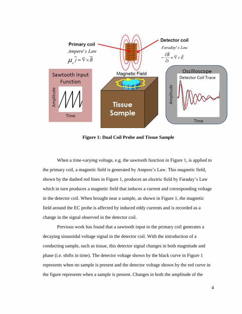
Figure 1: Dual Coil Probe and Tissue Sample

When a time-varying voltage, e.g. the sawtooth function in Figure 1, is applied to

the primary coil, a magnetic field is generated by Ampere’s Law. This magnetic field,

shown by the dashed red lines in Figure 1, produces an electric field by Faraday’s Law

which in turn produces a magnetic field that induces a current and corresponding voltage

in the detector coil. When brought near a sample, as shown in Figure 1, the magnetic

field around the EC probe is affected by induced eddy currents and is recorded as a

change in the signal observed in the detector coil.

Previous work has found that a sawtooth input to the primary coil generates a

decaying sinusoidal voltage signal in the detector coil. With the introduction of a

conducting sample, such as tissue, this detector signal changes in both magnitude and

phase (i.e. shifts in time). The detector voltage shown by the black curve in Figure 1

represents when no sample is present and the detector voltage shown by the red curve in

the figure represents when a sample is present. Changes in both the amplitude of the

5

peaks and the time between peaks and are detected using lock-in amplification.

Furthermore, the type of tissue brought near the probe affects the magnitude and phase

differently, so that lock-in amplification is able to differentiate between dissimilar types

of tissues.

2.3 Previous EC Probe Design

A previously described dual coil design, referred to as B1, has been successfully

used to detect the difference between normal and cancerous tissue [8]. B1 is wound with

32 gauge wire and has 2 layers on the primary coil side, 5 layers on the detector coil side,

a length of 0.66 in, an inner diameter of 0.216 in, and an outer diameter of 0.326 in [8].

Figure 2 shows B1 as well as a surgically excised liver metastasis specimen that has been

measured in three different locations with varying distance from the tumor (which is at

location 3) [Emily Sequin, personal communication, March 20, 2014].

Figure 2: Cancer Detection of an Excised Liver Metastasis

6

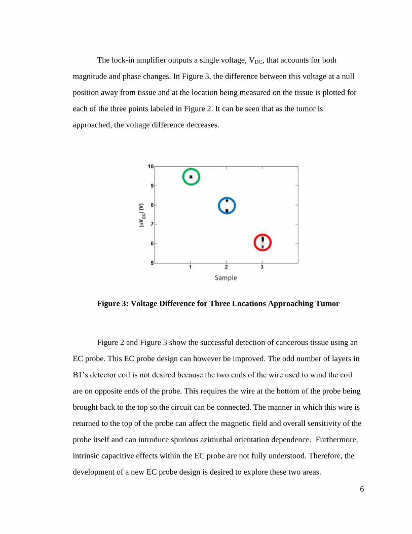
The lock-in amplifier outputs a single voltage, VDC, that accounts for both

magnitude and phase changes. In Figure 3, the difference between this voltage at a null

position away from tissue and at the location being measured on the tissue is plotted for

each of the three points labeled in Figure 2. It can be seen that as the tumor is

approached, the voltage difference decreases.

Figure 3: Voltage Difference for Three Locations Approaching Tumor

Figure 2 and Figure 3 show the successful detection of cancerous tissue using an

EC probe. This EC probe design can however be improved. The odd number of layers in

B1’s detector coil is not desired because the two ends of the wire used to wind the coil

are on opposite ends of the probe. This requires the wire at the bottom of the probe being

brought back to the top so the circuit can be connected. The manner in which this wire is

returned to the top of the probe can affect the magnetic field and overall sensitivity of the

probe itself and can introduce spurious azimuthal orientation dependence. Furthermore,

intrinsic capacitive effects within the EC probe are not fully understood. Therefore, the

development of a new EC probe design is desired to explore these two areas.

7

Chapter 3: Experimental Methods

3.1 Development of the C-Series of Probes

In order to investigate the effects of the number of detector layers and intrinsic

capacitance within the EC probe design, a new series of probes is developed and titled the

C-Series. These EC probes, labeled C1 through C4, are shown in Figure 4.

Figure 4: C-Series of EC Probes

The C-series of probes are similar to the B-series except for two main, systematic

differences. First, one detector layer is removed to allow for an even number of layers

8

and for the wire leads to be on the same end of the probe. B1 has 5 detector layers while

the C-Series has 4 detector layers. Furthermore, wire insulation thickness is varied in the

C-series to explore the effects of intra-coil capacitance. C1 and C4 are wound with 32

gauge wire ( McMaster, 7588K88) with a radial insulation thickness of 0.001 in, while

C2 and C3 are wound with 32 gauge wire obtained from Magnet Wire Supply (MWS, 32

SPN-155 RED NEMA MW80-C) with a radial insulation thickness of 0.0004 in.

The C-Series of EC probes are wound around a nylon core for two reasons. One, a

non-conducting central core is required for the probe because it operates with the use of a

magnetic field and any conducting material would alter this field. Two, a supporting

structure connected to the core allows the probe to be connected to fixtures such as

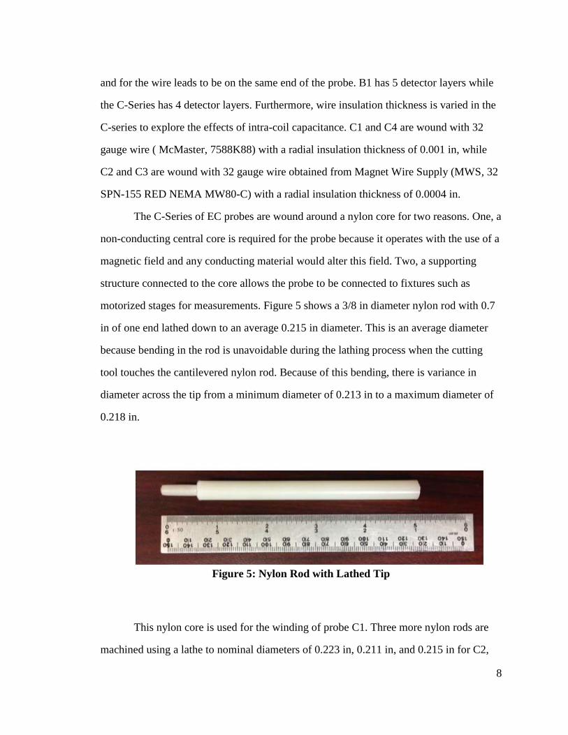
motorized stages for measurements. Figure 5 shows a 3/8 in diameter nylon rod with 0.7

in of one end lathed down to an average 0.215 in diameter. This is an average diameter

because bending in the rod is unavoidable during the lathing process when the cutting

tool touches the cantilevered nylon rod. Because of this bending, there is variance in

diameter across the tip from a minimum diameter of 0.213 in to a maximum diameter of

0.218 in.

Figure 5: Nylon Rod with Lathed Tip

This nylon core is used for the winding of probe C1. Three more nylon rods are

machined using a lathe to nominal diameters of 0.223 in, 0.211 in, and 0.215 in for C2,

9

C3, and C4 respectively with a tolerance of ±0.0001 in for all measurements. Each of

these machined cores also has a varying diameter across its profile due to bending of the

rod during the machining process, but the differences between maximum and minimum

diameter for each core (0.024in, 0.019in, and 0.012in respectively) are considered small.

Coils are wound using a clamp to hold the nylon rod while the 32 gauge wire is

hand-wound around the lathed tip. Figure 6 shows this process with the first layer of the

primary coil being wound around the nylon core. The start of each coil is at the right next

to the 3/8in end. Wrapping consistently and tightly packed to the left as far as possible

completes the first layer of the primary coil. Continuing wrapping the wire consistently

and tightly packing over this first layer and returning to the right, back to the start,

completes the second and final layer of the primary coil.

Figure 6: Wire Winding Process

After the two primary layers are completed, a layer of Clear Gloss 01 (Sally

Hansen Hard as Nails Color) nail polish is applied to the outside of the primary coil to

secure it when dried. The wire is then cut leaving enough extra length to connect to a

10

circuit board later. The detector coil is then wound around the primary coil using the

same procedure except with four layers. Starting at the right again, the detector coil’s first

layer is wound to the left, the second layer is wound to the right, the third layer is wound

to the left, and the fourth layer is wound to the right. After completion of the four layers

in the detector coil, a layer of the nail polish is applied and allowed to dry and then the

wire is cut. The final probe consists of two primary coil layers on the inside and four

detector coil layers on the outside, each with approximately 65 turns per layer. It should

be noted that while winding the outer layers, the act of winding the wire parallel becomes

increasingly difficult and some scatter winding is unavoidable.

The fabrication process is repeated for probes C2, C3, and C4. Probes C2 and C3

are wound as similarly as possible with MWS wire with the thinner insulation thickness,

while C1 and C4 are wound as similarly as possible with McMaster wire with the thicker

insulation thickness. The final inner and outer average diameters and lengths of each

probe are given in Table 1.

Table 1: Physical Dimensions of C-Series EC Probes (±0.0001 in Measurement

Tolerance)

C1 C2 C3 C4

Inner Diameter

(in)

0.215 0.223 0.211 0.215

Outer Diameter

(in)

0.328 0.313 0.310 0.310

Length (in) 0.685 0.684 0.642 0.651

11

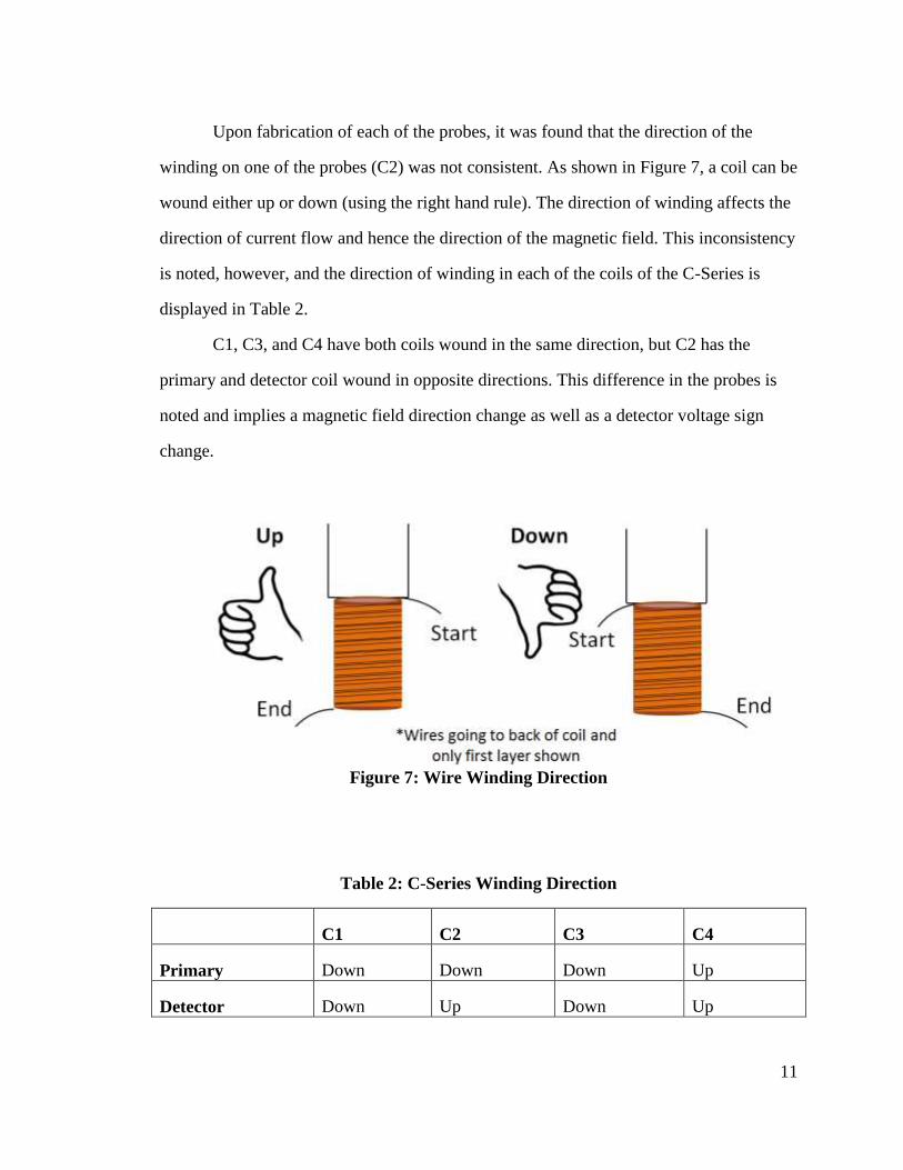
Upon fabrication of each of the probes, it was found that the direction of the

winding on one of the probes (C2) was not consistent. As shown in Figure 7, a coil can be

wound either up or down (using the right hand rule). The direction of winding affects the

direction of current flow and hence the direction of the magnetic field. This inconsistency

is noted, however, and the direction of winding in each of the coils of the C-Series is

displayed in Table 2.

C1, C3, and C4 have both coils wound in the same direction, but C2 has the

primary and detector coil wound in opposite directions. This difference in the probes is

noted and implies a magnetic field direction change as well as a detector voltage sign

change.

Figure 7: Wire Winding Direction

Table 2: C-Series Winding Direction

C1 C2 C3 C4

Primary Down Down Down Up

Detector Down Up Down Up

12

The primary coil has an inner and an outer lead wire and the detector coil has an

inner and an outer lead wire. The inner wire connects to the radially inward layer and the

outer wire connects to the radially outward layer. The four total lead wires of the probe

are covered with different colored shrink tubing and are soldered into a printed circuit

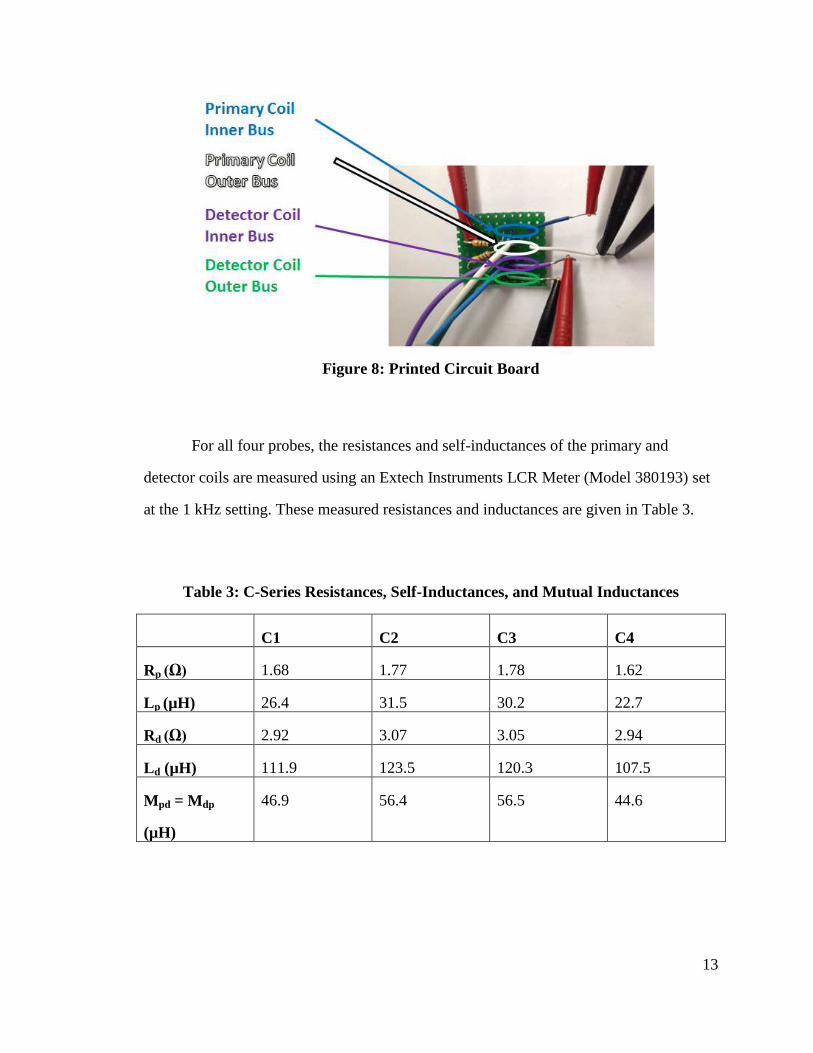
board (PCB) as shown in Figure 8. Each of these wires has its own bus on the circuit

board and a color code is used to differentiate between them. The inner wire of the

primary is blue, the outer wire of the primary is white, the inner wire of the detector is

purple, and the outer wire of the detector is green. The color of the shrink tubing used for

each wire coordinates with this color code, but the shrink tubing is not heated because it

holds more stiffness and support when it is unheated. In this manner, the shrink tubing

serves as a color code as well as a protective layer around the wire. Four small wires with

the same four colors are then soldered into their respective colored buses on the circuit

board as shown on the right in Figure 8. These wires allow for the easy connection of

micro-grabbers, which are also shown in Figure 8. Finally two 550 ballast resistors are

soldered into the PCB as shown in Figure 8. One resistor is soldered to the primary coil

inner bus and the other is soldered to the primary coil outer bus. This allows for easy

switching of the direction of the applied voltage in the primary coil without unsoldering

and re-soldering, which can affect the overall capacitance in the circuit. The soldering of

the PCB is repeated for all four C-Series probes.

In order to have a flat surface to contact tissue specimens, all four probes are then

placed in 1mm thick glass housing and secured with electrical tape. These glass housings,

shown in Figure 4, have large enough diameters that any envelopment of the tissue

around them during an experiment would not affect the measurement.

13

Figure 8: Printed Circuit Board

For all four probes, the resistances and self-inductances of the primary and

detector coils are measured using an Extech Instruments LCR Meter (Model 380193) set

at the 1 kHz setting. These measured resistances and inductances are given in Table 3.

Table 3: C-Series Resistances, Self-Inductances, and Mutual Inductances

C1 C2 C3 C4

Rp (Ω) 1.68 1.77 1.78 1.62

Lp (µH) 26.4 31.5 30.2 22.7

Rd (Ω) 2.92 3.07 3.05 2.94

Ld (µH) 111.9 123.5 120.3 107.5

Mpd = Mdp

(µH)

46.9 56.4 56.5 44.6

14

The mutual inductances of each of the probes are then calculated using a

MATLAB inductance calculator previously written for the dual coil probe design [10].

This calculator, given in Appendix A of this thesis, takes the probe length, wire diameter,

inner and outer diameter of each coil, number of turns, and number of layers as inputs

and calculates the self-inductances of the two coils and their mutual inductance as

outputs. For each probe the calculated self-inductances are within 5 µH of the actual

measured inductances. The measured self-inductances of the primary coils are 26.4, 31.5,

30.2, and 22.7 µH for C1, C2, C3, and C4 respectively. The measured self-inductances of

the detector coils are 111.9, 123.5, 120.3, and 107.5 µH for C1, C2, C3, and C4

respectively. The uncertainty in these inductance measurements is 0.1 µH. The calculated

mutual inductances for each of the C-Series probes are given in Table 3. The calculated

mutual inductances of the probes are 46.9, 56.4, 56.5, and 44.6 µH for C1, C2, C3, and

C4 respectively. It should be noted that mutual inductances Mpd and Mdp are taken to be

equal.

The capacitances of the coils are difficult to measure because they are small.

Previous studies have found that any capacitive buildup in the open circuit coil not

currently being measured will result in an unrealistically high value of the measured

capacitance [9]. The capacitances of the coils are therefore inferred by comparing with a

model.

3.2 Inferring Capacitance

Capacitance is inferred through the use of a model. In order to understand the

electrical properties of the EC probe and simulate the detector voltage signal, an electrical

circuit element model is used as shown in Figure 9.

15

Figure 9: EC Probe Electrical Circuit Model

The left side of the circuit in Figure 9 represents the primary coil of the probe

attached to the input voltage source through a ballast resistance. The primary coil is

represented by a resistor and inductor in parallel with a capacitor. The resistor accounts

for the conductivity of the wire, the inductor accounts for the rings of wire in the coil, and

the capacitance accounts for the charge build-up between windings as well as between

layers. The right side of the circuit represents the detector coil with the same electrical

elements of a resistor and inductor in parallel with a capacitor. At the bottom of the

diagram, an inductor and resistor represent the path of an eddy current in a sample. The

primary coil, detector coil, and eddy current all interact with each other through mutual

inductance. Because the primary and detector coils are inter-wound, they are mutually

coupled and because the magnetic field of the EC probe is affected by the eddy current in

the tissue, there is also mutual inductance between the tissue and the two coils.

16

When no sample is present, the bottom circuit elements become zero and the

model simplifies to only the primary and detector coil circuits linked with a single mutual

inductance assumed to be equal in both directions. Using this simplified electrical circuit

model of the EC probe, the differential equations (Eq. 1, 2, 3 and 4) relating the primary

coil to the detector coil can be written:

Equation 1: Primary Coil Current Law

Equation 2: Detector Coil Current Law

Equation 3: Primary Coil Voltage Law

Equation 4: Detector Coil Voltage Law

These differential equations can be numerically solved for the voltages and

currents in both the primary and detector coils. The simulated voltages of the primary and

detector coils can then be compared with experimental voltages obtained. Because all

parameters in the model besides the capacitances of each of the coils are measured or

calculated, capacitance can be adjusted until the simulated and experimental results

match.

Before actually inferring these capacitances, however, it is noted that because

there are two coils with two lead wires, there are a total of four possible lead wire

17

arrangements with how the function generator and oscilloscope or lock-in amplifier can

be connected to the probe.

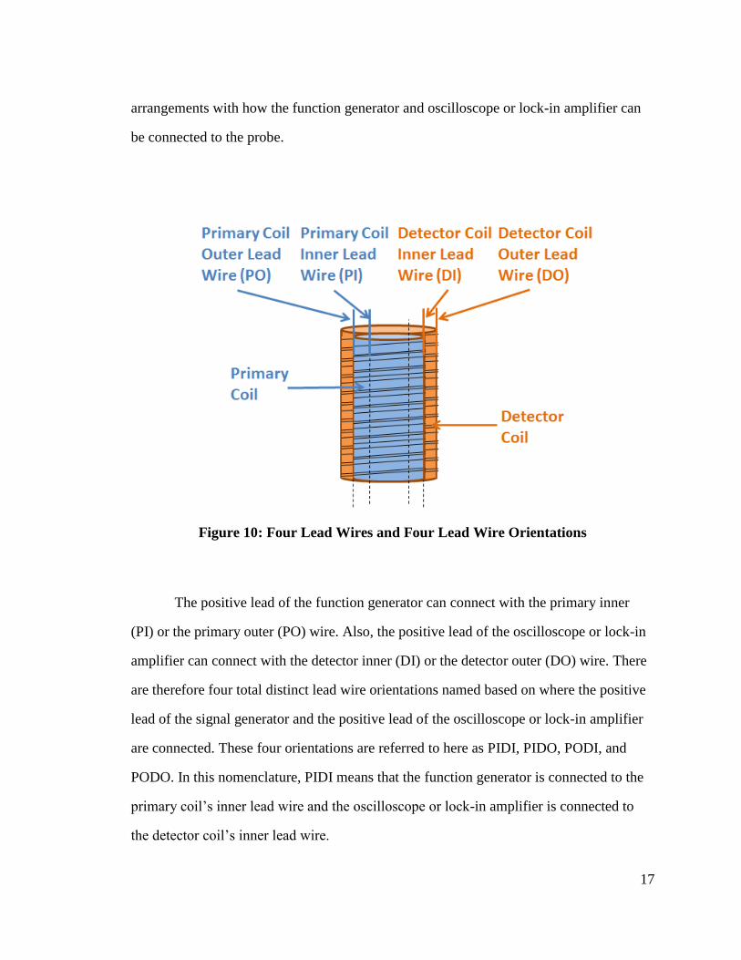
Figure 10: Four Lead Wires and Four Lead Wire Orientations

The positive lead of the function generator can connect with the primary inner

(PI) or the primary outer (PO) wire. Also, the positive lead of the oscilloscope or lock-in

amplifier can connect with the detector inner (DI) or the detector outer (DO) wire. There

are therefore four total distinct lead wire orientations named based on where the positive

lead of the signal generator and the positive lead of the oscilloscope or lock-in amplifier

are connected. These four orientations are referred to here as PIDI, PIDO, PODI, and

PODO. In this nomenclature, PIDI means that the function generator is connected to the

primary coil’s inner lead wire and the oscilloscope or lock-in amplifier is connected to

the detector coil’s inner lead wire.

18

Figure 11 shows the effect of changing orientations by monitoring the detector

voltage signal for the four lead wire orientations of C1. When switching between these

four lead wire orientations, not only is there a change in sign of the detector voltage

signal, but there is also a change in magnitude and phase because the peaks of the ringing

change in amplitude and shift in time. The PODI orientation in the top right quadrant of

Figure 11 has less voltage amplitude in the first peak but much longer ringing than the

PIDO orientation in the bottom left.

Figure 11: Detector Voltage Traces for C1 in All Orientations

It is important to be aware of how the probe is connected to the various

instruments due to the fact that there are multiple layers in each coil and the skin depth of

19

the magnetic field generated by each layer is limited. If the inner layer of the primary coil

is connected to the function generator (PI orientation), the magnetic field it creates will

not affect the detector coil as strongly as if the function generator was connected to the

primary coil’s outer layer (PO orientation). This is because in the former case of PI, the

magnetic field must permeate through the outer primary coil layer before interacting with

the windings of the detector layers. Because of this skin depth effect, there is a decrease

in magnitude of the magnetic field as it permeates through the extra coil layer.

In total, there are four possible orientations for a probe and capacitance can be

inferred for each of them. This is accomplished by connecting each probe in each

orientation, recording an experimental oscilloscope trace of the primary and detector

voltage traces, and comparing the experimentally measured voltages to simulated

voltages. These voltage traces are imported into MATLAB and compared (Appendix B).

Figure 12 shows the graphical interface used to infer the capacitance with primary and

detector voltage traces. All simulated inputs are known, measured, or calculated except

for the capacitances. Experimental inputs allow the user to choose which probe and

orientation to examine as well as whether the first peak in the detector voltage is positive

or negative. When the capacitances in the model are systematically varied so as to match

the experimental traces, the inferred capacitance of the probe is recorded.

20

Figure 12: MATLAB Graphical Interface to Infer Capacitance

In this procedure, it is noted that the magnitude of the peaks obtained in the

simulations are larger than the magnitude of the peaks recorded in the experiments.

Adjusting capacitance allows for the phase of the peaks to align, but in order to align the

magnitudes, detector resistance must be increased. Increasing this resistance decreases

the magnitude of the voltage peaks without altering their phase. The justification for

increasing the required resistance in the detector coil is that one needs to account for the

inductive impedance of the detector coil at the frequencies of interest (99 kHz) to the

measurement.

In the numerical model, the adjustment of capacitance is what is implemented in

order to align the phase of the experimental and simulated voltages. It is noted that the

best alignment of experimental and simulated voltage traces occur when primary and

detector capacitances are equal. This is not what would be expected for two coils with

different numbers of layers, but is an equivalent capacitance used to mimic the probe

21

characteristics. The inferred capacitances are thus recorded for each of the four probes

connected in each of the four lead wire orientations.

3.3 Experimental Apparatus

In order to conduct measurements on animal tissue with the C-Series of EC

probes, a system is setup to control the probe and collect the data. The experimental

apparatus used in this system is shown in Figure 13. A Hewlett Packard 33120A 15 MHz

function waveform generator is used to drive a 7 Vpp, 99 kHz, sawtooth waveform

through a 550 Ω ballast resistor and into the primary coil. Connected as shown in Figure

13, a Stanford Research System SR510 Lock-in Amplifier is used to measure both the

amplitude and phase of the detector signal relative to the reference signal from the

function generator. This lock-in amplifier is useful for this application because it is

capable of accurately measuring small signals by reducing noise [11]. The DC voltage

output from the lock-in is then connected to an Agilent DSO-X 2014A, 100 MHz,

Oscilloscope. Data from the oscilloscope is collected on a flash drive in CSV format and

transferred to a computer where it is saved and analyzed.

22

Figure 13: Experimental Apparatus for Data Acquisition

The SR510 Lock-In Amplifier is able to detect changes in both magnitude (Vi)

and phase (Ø) according to Equation 5. The settings for the lock-in amplifier when it is

used are given in Table 4.

Equation 5: Lock-In Amplifier Output Voltage

Where: Ae = 1 or 10 per the Expand setting

Av = 1/Sensitivity

Vi = magnitude of signal

Ø = phase between signal and reference

Vos = offset (not used)

23

Table 4: Lock-In Amplifier Settings

Option Setting

Input Signal Detector Coil

Voltage into

Channel A

Reference Signal 7 Vpp, 99 kHz

Sawtooth

Sensitivity 2mV

Dynamic

Resolution

High

All Offsets Off

Expand X1

Mode f

Trigger ~

Pre Time Constant 300ms

Post Time Constant 0.1s

3.4 Experimental Procedure

This section describes the procedures used to collect data in the experiments

reported here. Measurements on animal tissue specimens of pork and beef are taken for

all four probes in all four lead wire orientations described earlier. This allows the

determination of the orientation that produces maximum signal between null and tissue as

well as the orientation that offers maximum contrast between the two tissue specimens.

After determining the optimum orientation, an external capacitor is soldered in parallel

with the detector coil of each probe and measurements are repeated for the optimum

orientation with the external capacitance added ranging from 10pF to 100pF in 10pF

24

increments. The added parallel capacitance in the external circuit has been recently found

to optimize EC probe performance and overcome any drawbacks from the coil fabrication

process [Travis Jones, personal communication, January 27, 2014].

Animal tissue samples are obtained from the Giant Eagle grocery store. Pork Loin

Boneless Center Cut Chops and 80% Lean, 20% Fat Ground Chuck Beef are obtained

and allowed to warm to room temperature over the course of approximately one hour.

These two tissue samples are chosen because they have different morphological

structures: pork being a relatively homogeneous tissue and ground beef being an extruded

tissue packed together to have individual grains.

The pork tissue is then cut into two 1 in by 1 in by 0.5 in cubes and the ground

beef is hand formed into two similar 1 in by 1 in by 0.5 in cubes in order to have samples

of analogous volume. One pork cube is sealed in a storage bag and the two beef cubes are

sealed in a separate storage bag in order to preserve their freshness while the first

measurements are conducted on a pork sample without external capacitance. The other

pork sample and one of the beef samples are used for measurements where external

capacitance is added, while the other beef sample is measured without external

capacitance as well.

A grounding wire is placed horizontally across a plexiglass stage and the first

pork sample is placed on top of the wire in the center of the stage. Then plastic wrap is

wrapped neatly around the tissue and secured down with electrical tape. The plastic wrap

preserves the tissue over the course of the measurements and the tape prevents the plastic

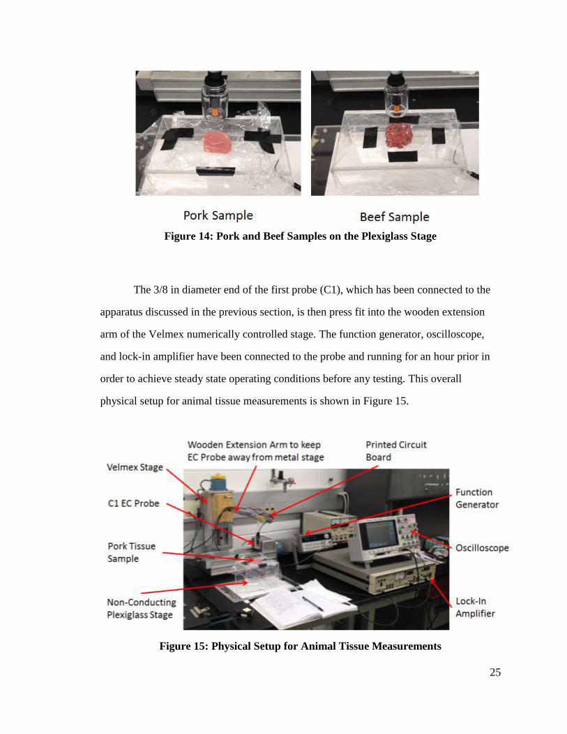
wrap from moving. The tissue setup on the plexiglass stage can be seen in Figure 14 for

both pork and beef samples.

25

Figure 14: Pork and Beef Samples on the Plexiglass Stage

The 3/8 in diameter end of the first probe (C1), which has been connected to the

apparatus discussed in the previous section, is then press fit into the wooden extension

arm of the Velmex numerically controlled stage. The function generator, oscilloscope,

and lock-in amplifier have been connected to the probe and running for an hour prior in

order to achieve steady state operating conditions before any testing. This overall

physical setup for animal tissue measurements is shown in Figure 15.

Figure 15: Physical Setup for Animal Tissue Measurements

26

Difficulties were encountered with fixturing using the Velmex stage.

Consequently, the Velmex stage was not used and the plexiglass stage with the sample

was manually raised up to the probe.

For the first probe (C1) and first orientation (PIDI), three repeated measurements

of pork tissue are recorded. First, the reference phase of the lock-in amplifier is adjusted

to produce an output voltage close to zero and the oscilloscope is set to start collecting

data. Three seconds of data are collected, and then the stage and sample are raised to the

bottom of the probe’s glass housing where three more seconds of data are collected. This

is repeated two more times for a total of three measurements with as constant a physical

force applied as possible. The oscilloscope is stopped from recording any more data and

the voltage trace from the lock-in amplifier is then saved. An example of the voltage

detected by the lock-in amplifier for the three repeated measurements is shown in Figure

16. The peaks represent the null state away from the tissue and the valleys represent

measurements taken on the tissue specimen.

Figure 16: Three Repeated Measurements of Pork using C1 in the PODI

Orientation

0 5 10 15 20-0.5

-0.45

-0.4

-0.35

-0.3

-0.25

-0.2

-0.15

Time (s)

Lock-

In V

oltag

e (

V)

27

The differences between successive peaks and valleys are then calculated for a

total of three measurements. The first, second, and third peaks are compared with the

first, second, and third valleys respectively to represent the three different voltage

changes obtained from the introduction of the tissue. This process of calculating voltage

change is accomplished by averaging 500 data points, or 0.2s of data, at the peaks and

valleys of the voltage data recorded by the lock-in amplifier. Data points are taken as far

away as possible from the transient voltage change due to tissue movement. The first

peak average voltage is then subtracted from the first valley average voltage to obtain the

first change in lock-in voltage due to tissue. This is repeated for all three measurements

for a total of three voltage changes. The average and 95% confidence interval of these

three measurements is then calculated using Equation 6 and the student t-distribution.

The t-distribution is used because the population standard deviation is unknown.

Equation 6: T-Distribution Confidence Interval

√

Where: = average of samples

t = t-score associated with α and n

α = 1 – confidence level (1-95% = 0.05 in this case)

n = number of samples (3 in this case)

s = sample standard deviation

For the pork sample, this process of three repeated measurements and confidence

interval calculation is followed for all four probes in all four orientations. The ground

beef sample is then placed on the stage and the measurement process is continued again

28

for all four probes in all four orientations. With 4 EC probes, 4 lead wire orientations, and

2 tissue samples, a total of 96 measurements and 32 confidence intervals are calculated

without external capacitance.

This data is then analyzed and the optimum orientation for each EC probe is

determined. The optimum orientation is chosen based on the best voltage contrast

between pork and beef specimens when at least a 0.1V signal is detected between null

and tissue. A 0.1V threshold is determined based on ability to distinguish between null

and tissue in the collected data because a difference in voltage of less than 0.1V is

relatively difficult to discern.

For probe C1, external capacitance is then added by soldering a variable

capacitor, shown in Figure 17, in parallel with the detector coil.

Figure 17: Variable Capacitor

Using the same procedure of three repeated measurements, measurements are

taken on the remaining pork and beef specimens for external capacitance varying from

10pF to 100pF with 10pF increments. With 4 EC probes, 1 optimum lead wire orientation

for each probe, 2 tissue samples, and 10 external capacitance increments, a total of 240

measurements and 80 confidence intervals are calculated with external capacitance.

29

Chapter 4: Results and Discussion

4.1 Comparison of B1 and C-Series EC Probes

The two systematic differences between B1 and the C-Series are number of

detector layers and insulation thickness. B1 has 5 detector layers while the C-Series has 4

detector layers. Furthermore, C1 and C4 have a radial insulation thickness of 0.001 in

while C2 and C3 have a radial insulation thickness of 0.0004 in. B1’s insulation thickness

is unknown but inferred to be 0.001 in by comparing the type of wire used with that

available in the laboratory where B1 was developed. Including these two main

differences between B1 and the C-Series, Table 5 compares the physical properties of all

of these EC probes.

30

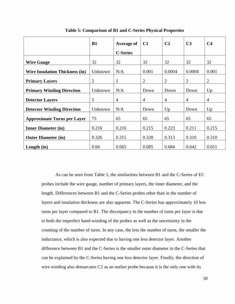
Table 5: Comparison of B1 and C-Series Physical Properties

B1 Average of

C-Series

C1 C2 C3 C4

Wire Gauge 32 32 32 32 32 32

Wire Insulation Thickness (in) Unknown N/A 0.001 0.0004 0.0004 0.001

Primary Layers 2 2 2 2 2 2

Primary Winding Direction Unknown N/A Down Down Down Up

Detector Layers 5 4 4 4 4 4

Detector Winding Direction Unknown N/A Down Up Down Up

Approximate Turns per Layer 75 65 65 65 65 65

Inner Diameter (in) 0.216 0.216 0.215 0.223 0.211 0.215

Outer Diameter (in) 0.326 0.315 0.328 0.313 0.310 0.310

Length (in) 0.66 0.665 0.685 0.684 0.642 0.651

As can be seen from Table 5, the similarities between B1 and the C-Series of EC

probes include the wire gauge, number of primary layers, the inner diameter, and the

length. Differences between B1 and the C-Series probes other than in the number of

layers and insulation thickness are also apparent. The C-Series has approximately 10 less

turns per layer compared to B1. The discrepancy in the number of turns per layer is due

to both the imperfect hand-winding of the probes as well as the uncertainty in the

counting of the number of turns. In any case, the less the number of turns, the smaller the

inductance, which is also expected due to having one less detector layer. Another

difference between B1 and the C-Series is the smaller outer diameter in the C-Series that

can be explained by the C-Series having one less detector layer. Finally, the direction of

wire winding also demarcates C2 as an outlier probe because it is the only one with its

31

primary and detector coils wound in opposite directions. These different winding

directions would be expected to affect the magnetic field and detector signal, as is found

and discussed in the next section.

The electrical characteristics of B1 and the C-Series coils can be compared as

well. Table 6 shows the electrical properties of B1 and the C-Series. It should be noted

that for the C-Series, the effective capacitances have maximum and minimum values

since lead wire orientation affects intrinsic capacitance, as will be shown in the next

section.

Table 6: Comparison of B1 and C-Series Electrical Properties

B1 Average of

C-Series

C1 C2 C3 C4

Rb

(Ω) 830 550 550 550 550 550

Rp

(Ω) 1.98 1.71 1.68 1.77 1.78 1.62

Lp

(μH) 38.7 27.7 26.4 31.5 30.2 22.7

Cp

(pF) 235 Min: 236

Max: 471

Min: 215

Max: 375

Min: 260

Max: 520

Min: 260

Max: 595

Min: 210

Max: 395

Rd

(Ω) 5.59 3.00 2.92 3.07 3.05 2.94

Ld

(μH) 330 115.8 111.9 123.5 120.3 107.5

Cd

(pF) 235 Min: 236

Max: 471

Min: 215

Max: 375

Min: 260

Max: 520

Min: 260

Max: 595

Min: 210

Max: 395

Mpd

=Mdp

(μH) 94.1 51.1 46.9 56.4 56.5 44.6

The main similarities in electrical properties between the B1 and the C-Series are

the primary resistance and inductance, which are expected because both probes have 2

layers in the primary coil. The slight decrease in the primary resistance and inductance of

32

the C-Series can be accounted for by approximately 10 less turns per layer. This as well

as one less layer in the detector coil explains why the C-Series has less detector coil

resistance and inductance. It is important to note that the removal of one detector layer

drastically reduced the inductance of the detector coil by almost a third and the mutual

inductance by half. B1 has a detector coil inductance on the order of 300 μH while the

average detector coil inductance of the C-Series is on the order of 100 μH. Furthermore,

B1 has a mutual inductance of approximately 100 μH while the C-Series has a mutual

inductance of approximately 50 μH. It is also important to note that when comparing

wire insulation thickness, C2 and C3 have thinner insulation thickness and higher

inferred capacitance compared to C1 and C4. This is expected based on the equation for

parallel plate capacitance, Equation 7. Even though this equation is not strictly valid for

estimating the intrinsic capacitance within the coils, it can be used to infer that a thinner

insulation would lead to decreasing the distance, L, between charged wires and increasing

capacitance. The capacitances do not directly correlate however because the insulation

thickness was decreased by a factor of 2.5 but the inferred capacitance only increased by

approximately 20-40%. This discrepancy is due to the significant assumption made when

comparing the EC probe to a parallel plate capacitor.

Equation 7: Parallel Plate Capacitance

Where: =dielectric permittivity of the medium

A=Area of charged surface

L=Distance between areas

33

The final significant difference between B1 and the C-Series is the decrease in

ballast resistance. The C-Series requires a lower ballast resistance of 550Ω compared to

the 830Ω ballast resistance of B1 to obtain a similar magnitude in detector voltage signal.

This is expected due to the smaller mutual inductance of the C-Series. Because the

primary and detector coils in the C-Series of probes are less mutually coupled, the

primary coil affects the detector coil less and a lower magnitude signal is obtained in the

detector voltage. To counteract this, a smaller ballast resistance is used.

4.2 Capacitive Effects, Lead Wire Orientation, and Animal Tissue Measurements

Upon investigating the inferred capacitances for each probe in the C-Series, it is

found that the inferred capacitance depends on the lead wire orientation of how the probe

is connected to the function generator and the oscilloscope or lock-in amplifier. Figure 18

through 21 show the detector voltage traces for all four orientations of probes C1 through

C4 respectively when they are away from tissue or any sample. As can be seen from

these figures, changing the orientation of the probe affects more than just the sign of the

detector voltage signal. Both the magnitude of the peaks and the time between peaks are

affected when orientation is changed. Furthermore, because the phase or time between

peaks changes, there is a noticeable change in inferred capacitance with a change in lead

wire orientation. When lead wire orientation is changed, the percent difference between

maximum and minimum inferred capacitance is 54%, 67%, 78%, and 61% for C1, C2,

C3, and C4 respectively.

A common relationship between orientation and capacitance is found. For probes

C1, C3, and C4, the PODI orientation is found to have the most elongated or maximum

ringing while the PODO orientation is found to have minimum ringing. Additionally, in

these three probes the PODI orientation has the largest inferred capacitance while the

PODO orientation has the smallest inferred capacitance.

34

C2 does not follow this trend, however, because of the direction in which its coils

are wound. Because the primary and detector coils of C2 are wound in opposite

directions, the magnetic field it produces and the mutual coupling between the coils result

in different detector voltage traces for each lead wire orientation. For C2, the maximum

ringing and capacitance are found in the PIDI orientation while the minimum ringing and

capacitance are found in the PIDO orientation.

When examining all C-Series probes as a whole, it is noted that as lead wire

orientation changes, capacitance and therefore the amount of ringing and magnitude of

peaks change. Moreover, certain orientations maximize or minimize capacitance and

consequently ringing.

Figure 18: C1 - Detector Voltage, Inferred Capacitance, and 95% CIs for Tissues

35

Figure 19: C2 - Detector Voltage, Inferred Capacitance, and 95% CIs for Tissues

Figure 20: C3 - Detector Voltage, Inferred Capacitance, and 95% CIs for Tissues

36

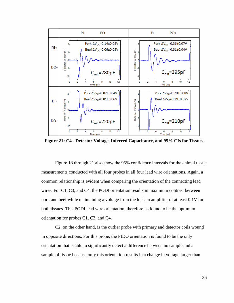
Figure 21: C4 - Detector Voltage, Inferred Capacitance, and 95% CIs for Tissues

Figure 18 through 21 also show the 95% confidence intervals for the animal tissue

measurements conducted with all four probes in all four lead wire orientations. Again, a

common relationship is evident when comparing the orientation of the connecting lead

wires. For C1, C3, and C4, the PODI orientation results in maximum contrast between

pork and beef while maintaining a voltage from the lock-in amplifier of at least 0.1V for

both tissues. This PODI lead wire orientation, therefore, is found to be the optimum

orientation for probes C1, C3, and C4.

C2, on the other hand, is the outlier probe with primary and detector coils wound

in opposite directions. For this probe, the PIDO orientation is found to be the only

orientation that is able to significantly detect a difference between no sample and a

sample of tissue because only this orientation results in a change in voltage larger than

37

0.1V. This PIDO orientation is considered the optimum orientation for C2 even though

only 0.01V of contrast between pork and beef is discernable.

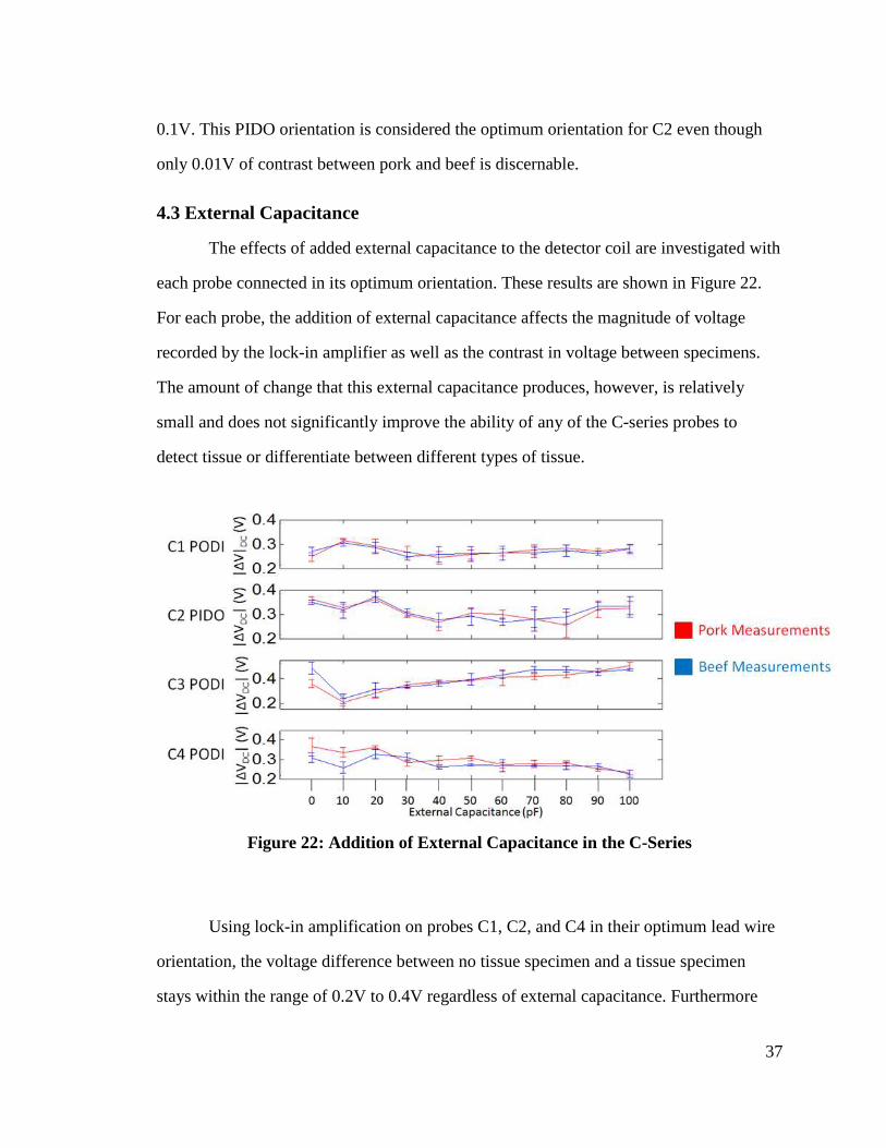
4.3 External Capacitance

The effects of added external capacitance to the detector coil are investigated with

each probe connected in its optimum orientation. These results are shown in Figure 22.

For each probe, the addition of external capacitance affects the magnitude of voltage

recorded by the lock-in amplifier as well as the contrast in voltage between specimens.

The amount of change that this external capacitance produces, however, is relatively

small and does not significantly improve the ability of any of the C-series probes to

detect tissue or differentiate between different types of tissue.

Figure 22: Addition of External Capacitance in the C-Series

Using lock-in amplification on probes C1, C2, and C4 in their optimum lead wire

orientation, the voltage difference between no tissue specimen and a tissue specimen

stays within the range of 0.2V to 0.4V regardless of external capacitance. Furthermore

38

the contrast between the two tissue specimens for each of these probes is even smaller.

Without external capacitance, C3 in the PODI orientation offered the best contrast of

0.14V between pork and beef tissue samples. With the addition of external capacitance,

however, this contrast becomes smaller and the signal of detecting tissue varied from

0.2V to 0.5V. With these results, it can be seen that the addition of external capacitance

in the detector coil has a minimal effect on both tissue detection as well as contrast

between tissue samples.

In order to investigate why external capacitance has minimal effect, C1 is

examined in the optimum PODI orientation. The primary coil is attached to the function

generator as usual, but the detector coil is attached to the oscilloscope directly without

lock-in amplification. The original detector voltage trace without external capacitance

when no sample is present is shown in green in Figure 23. The external variable capacitor

is then soldered to the detector coil and set to a low setting of 10pF. The new detector

voltage trace when no sample is present is shown in blue in Figure 23. Finally, the

variable capacitor is set to a high setting of 100pF and the detector trace without a sample

is obtained as shown in red in Figure 23.

39

Figure 23: Effect of External Capacitance on Detector Voltage

By examining the effect of external capacitance in Figure 23, it can be seen that

simply soldering the variable capacitor to the detector coil affects capacitance. From

green to blue in Figure 23, the addition of the external variable capacitor decreases

ringing and shifts the peaks left. As explained in Section 4.2, however, the addition of

capacitance in the detector coil elongates ringing. When the variable capacitor set to 10pF

is added, a change in the capacitance of the solder in the circuit is the only explanation

for a decrease in detector voltage ringing. When the variable capacitor is then increased

to 100pF, the detector voltage then elongates as expected. At this maximum external

capacitance however, the ringing in the detector voltage only lasts approximately 7.5µs

and does not last the entire duty cycle of the 99kHz input function which is slightly over

10µs.

0 2 4 6 8 10

-1.5

-1

-0.5

0

0.5

1

1.5

2

2.5

Time (s)

Dete

cto

r V

oltage (

V)

0pF

10pF

100pF

40

Chapter 5: Summary and Conclusions

5.1 Removing a Detector Coil Layer

The most significant difference between B1 and the C-Series is the number of

detector coil layers. B1 contains 5 layers and the C-Series contains 4 layers in the

detector coil. Because of this decrease in detector coil layers, the inductance of the

detector coil drastically decreases from 330µH in B1 to an average of 116µH in the C-

Series. The effect that this decrease in inductance has is seen when comparing the

detector voltage traces of B1 and the C-Series. Figure 24 shows how the ringing in the

detector voltage for B1 lasts significantly longer than that in the C-Series.

Figure 24: Detector Voltage Ringing in B1

41

In B1, the ringing lasts the whole duty cycle of the input function and even has a

visible peak intersecting with the first peak of the next duty cycle. Removing a single

layer of the detector coil significantly decreased the elongation of ringing in the detector

coil voltage.

5.2 Wire Insulation Thickness

The insulation of the wire used to wind the probe also affects the design of the EC

probe. This is evident when comparing probes C1 and C4 to probes C2 and C3 which

have 2.5 times thinner wire insulation. The inferred capacitance of C2 and C3 are higher

than those of C1 and C4 for each of the four lead wire orientations. This is expected,

however, when considering Equation 7 for parallel plate capacitance. Bringing the

conducting cores of the wires closer together with thinner insulation thickness should

increase capacitance. This increase in capacitance elongates the ringing in the detector

coil. This can be seen by comparing C3 and C4 in the PODI orientation. When in this

orientation, the ringing in C3, shown in the upper right quadrant of Figure 20, lasts

significantly longer than that of C4, shown in the upper right quadrant of Figure 21. As

wire insulation thickness decreases, inferred capacitance increases and detector voltage

ringing is elongated.

5.3 Orientation of Lead Wires

The manner in which the EC probe is connected to the function generator and

oscilloscope or lock-in amplifier is another factor that affects inferred capacitance and

ringing in the detector voltage. Figure 18 through 21 show that different lead wire

orientations result in different inferred capacitance and amounts of ringing. For probes

C1, C3, and C4, maximum inferred capacitance and maximum ringing were found for the

PODI orientation. Furthermore, this lead wire orientation also resulted in maximum

contrast between animal tissue samples. For the C-Series of EC probes, the orientation

42

with the highest inferred capacitance rings the most in the detector voltage and is able to

differentiate between animal tissues best.

5.4 External Capacitive Effects

The addition of external capacitance to the detector coil is another manner in

which the ringing features can be elongated. Figure 23 shows that as external capacitance

is increased from 10pF to 100pF, the peaks in the detector voltage trace shift to the right.

This added capacitance in the external circuit does not increase signal or contrast in the

C-Series of probes, however. As seen in Figure 22, varying capacitance from 10pF to

100pF does not markedly improve any of the probes ability to detect tissue or

differentiate between different types of tissue.

Addition of external capacitance to the C-series of probes did not improve their

sensitivity. This result can be explained by comparing Figure 23 with Figure 24. In

Figure 23, the ringing of C1 never exceeds approximately 7.5µs while in Figure 24 the

ringing of B1 not only lasts the full duty cycle of the input function (slightly over 10µs),

but it also runs into and affects the first peak of the next duty cycle. Current studies with

B1 have shown that external capacitance does affect the ability of B1 to detect different

tissues. Because the ringing in the C-Series is not as elongated as that in B1, however, the

effect of external capacitance on the probes in the C-Series is not as significant.

5.5 Comparison of Tissue Measurements with B1 and C-Series

When comparing B1 and the C-Series in ability to detect and differentiate

between different types of tissue, B1 is significantly better. Comparing Figure 3 and

Figure 22 shows that B1 not only is capable of producing larger voltages from the lock-in

amplifier, but is also more capable of discerning between different tissue samples. Figure

3 shows that when a tissue specimen is introduced to B1, the voltage from the lock-in

amplifier changes by a maximum of approximately 9.5V. Figure 22, on the other hand,

43

shows that the the C-Series voltage changes by a maximum of approximately 0.5V when

C3 is connected in the PODI orientation. Figure 3 also shows that B1 is capable of

discerning dissimilar tissue samples by a maximum of approximately 3.5V. Figure 22,

alternatively, shows that the C-Series is is only capable of discerning dissimilar tissue

samples by a maximum of approximately 0.15V. In general, B1 offers better signal near

tissue as well as better contrast between different tissue specimens. An explanation for

this is the significant change in detector voltage signal when a layer is removed as

discussed in Section 5.1.

44

Chapter 6: Recommendations for Future Work

6.1 Inferring Coil Capacitances

In this study, the capacitances of the C-Series of EC probes are inferred by

comparing simulated and experimental voltages in the primary and detector coil when a 7

Vpp, 99 kHz sawtooth function is input to the primary coil. When the capacitance is

adjusted to match predictions from the circuit element model and experimental results,

there is no starting point for the inferred capacitance. A possible way of obtaining this

initial inferred capacitance is by examining the two coils of the probe individually. One

could apply a 1 kHz sine wave to the primary coil, record the experimental voltage

response through an oscilloscope, and repeat for the detector coil. Then the model would

be able to infer capacitance for each coil in the probe independently. Moreover, because

the inductances of the coils are measured with an LCR meter at 1 kHz, the measured

inductances would be closer to the actual experimental inductances. In this work,

measured inductances are obtained at 1 kHz, but are implemented in simulated results at

99 kHz. Because the inductance can be frequency dependent, it would be better to use the

measured inductance values at the same frequency of 1 kHz when comparing simulations

and experimental results. This suggested method of inferring coil capacitances would

offer an initial inferred capacitance for both coils rather than finding the two coils’

capacitances to be the same as is found in this study. Furthermore, by inferring coil

capacitance in this manner, the frequency dependence of capacitance in the probe could

be examined.

45

6.2 Adding Detector Coil Layers

As explained in Section 5.1, the main difference between B1 and the C-Series of

EC probes is the removal of a detector coil layer. B1 has 5 detector coil layers and the C-

Series has 4 detector coil layers. One layer is removed in the design of the C-Series to

allow all lead wires from the probe to be on one side. The removal of this layer, however,

significantly decreased the inductance of the detector coil from 330µH in B1 to an

average of 116µH in the C-Series. This drastic decrease in inductance shortened the

ringing in the detector coil and stopped the last peak from interacting with the first peak

in the next duty cycle of the input function. It is suggested to add more layers to the EC

probe design to elongate the ringing in the detector coil voltage. An even number of

detector coil layers of 6 would allow this ringing to affect the next duty cycle while still

maintaining the ability to have all lead wires on the same side of the probe. This

increased number of detector coil layers would increase the inductance of the detector

and elongate ringing. This could possibly detect more signal between no sample and

tissue as well as better differentiate between tissue specimens.

46

Bibliography

[1] "SEER Stat Fact Sheets: All Cancer Sites." National Cancer Institute. Surveillance

Epidemiology and End Results. Web. 16 Nov 2013.

<http://seer.cancer.gov/statfacts/html/all.html>.

[2] Povoski, Stephen. "Antigen-Directed Cancer Surgery for Primary Colorectal Cancer: 15-

Year Survival Analysis." Surgical Oncology. (2012): n. page. Print.

[3] Frangioni, John. "The Problem is Background, not Signal."Molecular Imaging. 8.6

(2009): 303-304. Print.

[4] De Grand, Alec & Frangioni, John. "An Operational Near-Infrared Fluorescence

Imaging System Prototype for Large Animal Surgery." Technology in Cancer

Research & Treatment. 2.6 (2003): n. page. Print.

[5] Halter, Ryan. "Electrical Impedance Spectroscopy of the Human Prostate." IEEE

Transactions on Biomedical Engineering. 54.7 (2007): n. page. Print.

[6] Weinberg, Robert. The Biology of Cancer, Garland Science, Taylor & Francis, New

York, 2007.

[7] Lin, Eugene & Alavi, Abass. (2005). PET and PET/CT. New York: Thieme Medical

Publishers, Inc.

[8] Wilson, Michelle. Design and Fabrication of an Electromagnetic Probe for Biomedical

Applications, M.S. Thesis, The Ohio State University, 2011.

[9] Sequin, Emily. Imaging of Cancer in Tissues Using an Electromagnetic Probe, M.S.

Thesis, The Ohio State University, 2009.

[10] McFerran, Jennifer. An Electromagnetic Method for Cancer Detection, PhD

Dissertation. The Ohio State University, 2009.

[11] Stanford Research Systems. (1989). Model SR510 Lock-In Amplifier. Sunnyvale, CA:

Stanford Research Systems.

47

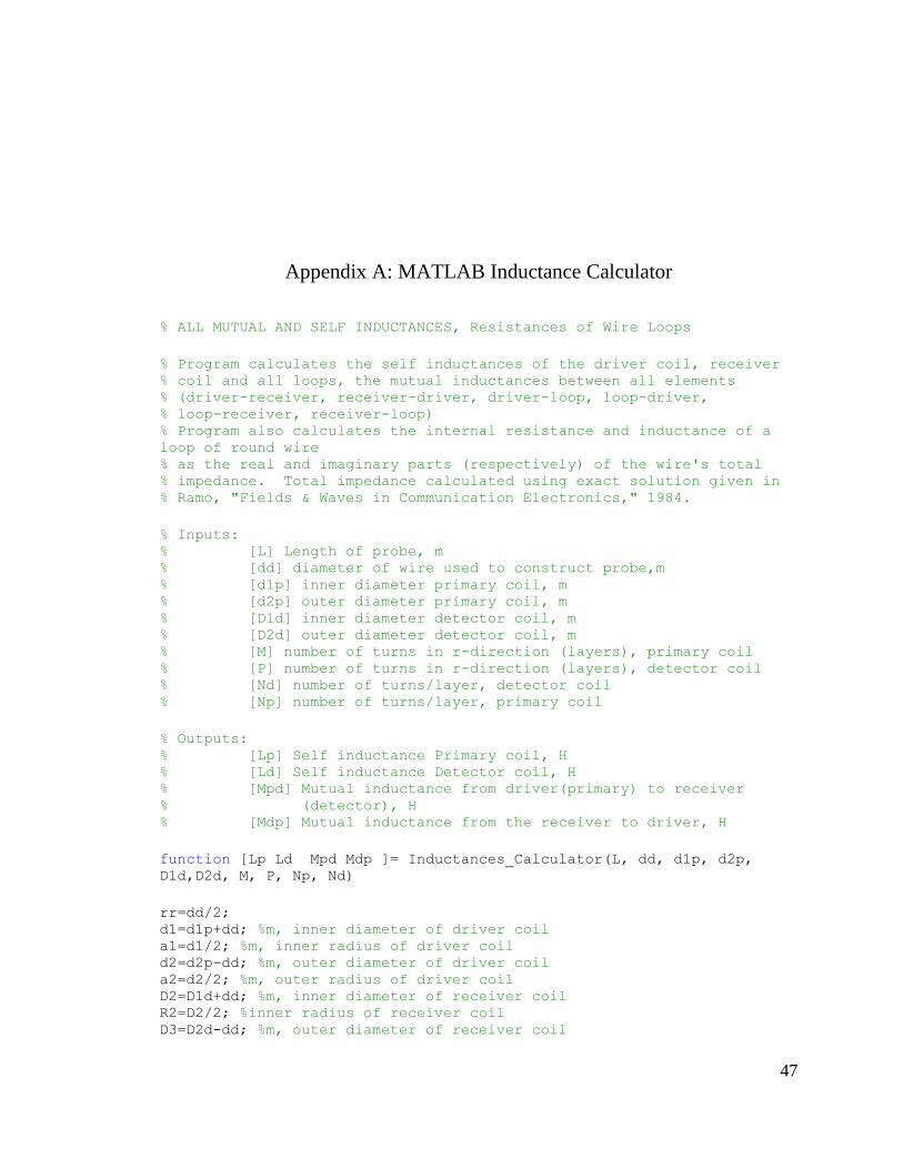
Appendix A: MATLAB Inductance Calculator

% ALL MUTUAL AND SELF INDUCTANCES, Resistances of Wire Loops

% Program calculates the self inductances of the driver coil, receiver % coil and all loops, the mutual inductances between all elements % (driver-receiver, receiver-driver, driver-loop, loop-driver, % loop-receiver, receiver-loop) % Program also calculates the internal resistance and inductance of a

loop of round wire % as the real and imaginary parts (respectively) of the wire's total % impedance. Total impedance calculated using exact solution given in % Ramo, "Fields & Waves in Communication Electronics," 1984.

% Inputs: % [L] Length of probe, m % [dd] diameter of wire used to construct probe,m % [d1p] inner diameter primary coil, m % [d2p] outer diameter primary coil, m % [D1d] inner diameter detector coil, m % [D2d] outer diameter detector coil, m % [M] number of turns in r-direction (layers), primary coil % [P] number of turns in r-direction (layers), detector coil % [Nd] number of turns/layer, detector coil % [Np] number of turns/layer, primary coil

% Outputs: % [Lp] Self inductance Primary coil, H % [Ld] Self inductance Detector coil, H % [Mpd] Mutual inductance from driver(primary) to receiver % (detector), H % [Mdp] Mutual inductance from the receiver to driver, H

function [Lp Ld Mpd Mdp ]= Inductances_Calculator(L, dd, d1p, d2p,

D1d,D2d, M, P, Np, Nd)

rr=dd/2; d1=d1p+dd; %m, inner diameter of driver coil a1=d1/2; %m, inner radius of driver coil d2=d2p-dd; %m, outer diameter of driver coil a2=d2/2; %m, outer radius of driver coil D2=D1d+dd; %m, inner diameter of receiver coil R2=D2/2; %inner radius of receiver coil D3=D2d-dd; %m, outer diameter of receiver coil

48

R3=D3/2; %m, outer radius of receiver coil

% EM properties mu0=4*pi*10^(-7); %V*sec/A/m, magnetic permittivity of vacuum I=1;%A, current (NB: all inductance values independent of current,

since it %divides out at the end

% SELF INDUCTANCES-----------------------------------------------------

--- % 1. Driver coil Z=linspace(0,L,Np); a=linspace(a1,a2,M);

clear flux_single_turn flux A k2 K E for e=1:M %r-direction, driver coil for f=1:Np %z-direction, driver coil for i=1:M %r-direction, driver coil for j=1:Np %z-direction, driver coil k2=4*a(i)*(a(e)-rr)*((a(i)+a(e)-rr)^2+(Z(f)-Z(j))^2)^(-

1); [K,E] = ellipke(k2); A=mu0*I/pi/sqrt(k2)*sqrt(a(i)/(a(e)-rr))*((1-.5*k2)*K-

E); flux_single_turn(i,j)=2*pi*(a(e)-rr)*A; end end flux(e,f)=sum(sum(flux_single_turn)); end end Lp=sum(sum(flux))/I %calculated self inductance of driver

%2. Receiver coil R=linspace(R2,R3,P); %receiver coil ZZ=linspace(0,L,Nd); %receiver coil

clear flux_single_turn flux A k2 K E for e=1:P %r-direction, receiver coil for f=1:Nd %z-direction, receiver coil for i=1:P %r-direction, receiver coil for j=1:Nd %z-direction, receiver coil k2=4*R(i)*(R(e)-rr)*((R(i)+(R(e)-rr))^2+(ZZ(f)-

ZZ(j))^2)^(-1); [K,E] = ellipke(k2); A=mu0*I/pi/sqrt(k2)*sqrt(R(i)/(R(e)-rr))*((1-.5*k2)*K-

E); flux_single_turn(i,j)=2*pi*(R(e)-rr)*A; end end flux(e,f)=sum(sum(flux_single_turn)); end end

Ld=sum(sum(flux))/I %calculated self inductance of receiver

49

% MUTUAL INDUCTANCES---------------------------------------------------

--- %1. Driver to receiver clear flux_single_turn flux A k2 K E for e=1:P %r-direction, receiver coil for f=1:Nd %z-direction, receiver coil for i=1:M %r-direction, driver coil for j=1:Np %z-direction, driver coil k2=4*a(i)*R(e)*((a(i)+R(e))^2+(ZZ(f)-Z(j))^2)^(-1); [K,E] = ellipke(k2); A=mu0*I/pi/sqrt(k2)*sqrt(a(i)/R(e))*((1-.5*k2)*K-E); flux_single_turn(i,j)=2*pi*R(e)*A; end end flux(e,f)=sum(sum(flux_single_turn)); end end

Mpd=sum(sum(flux))/I

%2. Receiver to driver clear flux_single_turn flux A k2 K E for i=1:M %r-direction, driver coil for j=1:Np %z-direction, driver coil for e=1:P %r-direction, receiver coil for f=1:Nd %z-direction, receiver coil k2=4*R(e)*a(i)*((R(e)+a(i))^2+(Z(j)-ZZ(f))^2)^(-1); [K,E] = ellipke(k2); A=mu0*I/pi/sqrt(k2)*sqrt(R(e)/a(i))*((1-.5*k2)*K-E); flux_single_turn(e,f)=2*pi*a(i)*A; end end flux(i,j)=sum(sum(flux_single_turn)); end end Mdp=sum(sum(flux))/I

50

Appendix B: MATLAB Code used to Infer Capacitance

Runner Function

This function is used to open the graphical interface. function Detector_Runner_Comparison_One_Plot clear all; close all; clc;

%setup main figure mainfig = figure(1); set(mainfig,'Position',[10 60 1900 930]); set(mainfig,'tag','mainfig'); set(mainfig,'Toolbar','figure')

%set font sizes ud.design.Heading = 40; %40 for Scott Lab 40 for laptop ud.design.Label = 20; %20 for Scott Lab 15 for laptop ud.design.Text = 15; %15 for Scott Lab 10 for laptop ud.design.Box = 12; %12 for Scott Lab 10 for laptop

subplot(1,1,1) set(subplot(1,1,1),'OuterPosition',[0.1 0.02 0.9 0.9]); xlabel('Time (s)','FontSize',ud.design.Label) ylabel('Voltage (V)','FontSize',ud.design.Label) set(gca,'fontsize',ud.design.Label) title('Experimental and Simulated Voltages v

Time','FontSize',ud.design.Label) grid on

%Initialize design parameters with C1 constants (capacitance guesses) ud.design.Points= 10000; %data points per period ud.design.Wav = 1; %sawtooth ud.design.Amp = 7; %volts ud.design.Freq = 99; %kHz ud.design.Rb = 578.2; %ohms ud.design.Cp = 300*10^-12; %farads ud.design.Rp = 1.68; %ohms ud.design.Lp = 26.4*10^-6; %henries ud.design.Cd = 300*10^-12; %farads ud.design.Rd = 2.92; %ohms ud.design.Ld = 111.9*10^-6; %henries ud.design.Mpd = 46.879*10^-6; %henries ud.design.Probe = 1; %C1

51

ud.design.HO = 1; %PI DI ud.design.Sign = 1; %positive ud.design.Data=xlsread('scope_01_pidi.xlsx','A3:E20002'); %1st data set TimeStep=1/(ud.design.Freq*1000)/ud.design.Points; LastTime=6/(ud.design.Freq*1000); ud.design.InputTime=(0:TimeStep:LastTime); Max=ud.design.Amp/2; FreqTime=2*pi*ud.design.Freq*1000*ud.design.InputTime; ud.design.InputVoltage=Max*sawtooth(FreqTime,1);

%%%%%%%%%%%%%%%%%%%%%%%%%%%% %%%%% UIcontrols below %%%%% %%%%%%%%%%%%%%%%%%%%%%%%%%%%

%left bound for text xtext = .035; %upper bound for text ytext = .8; %width of textbox wtext = .075; %height of textbox htext = .02; %vertical spacing ytextspace = .03; %left bound for edits xedit = xtext + .08; %width of edits wedit = .05;

%Headings ud.obj.Title = uicontrol('Style','text','string',... 'Eddy Current Probe Model','Units','normalized',... 'Position',[.25 .9 .5 .05],'BackgroundColor',[0.8 0.8 0.8],... 'FontSize',ud.design.Heading,'FontName','Stencil'); ud.obj.uiBanner = uicontrol('Style','text','string',... 'Design Parameters','Units','normalized','Position',... [xtext-.01 ytext+ytextspace wtext+.075 htext+.01],'FontSize',... ud.design.Label,'BackgroundColor',[0.8 0.8 0.8]);

%Waveform ud.obj.uiWav = uicontrol('Style', 'popup','Units','normalized',... 'String','Sawtooth|Square|Sine|O-Scope','Position',... [xedit ytext wedit htext],'FontSize',ud.design.Box,'Callback',

@setWav); ud.obj.uiWavtxt = uicontrol('Style','text','string','Waveform',... 'HorizontalAlignment','left','Units','normalized',... 'Position',[xtext ytext wtext htext],'FontSize',ud.design.Text,... 'BackgroundColor',[0.8 0.8 0.8]);

%Amplitude ud.obj.uiAmp = uicontrol('Style','edit','string',ud.design.Amp,... 'Units','normalized','Position',... [xedit ytext-ytextspace wedit htext],'FontSize',ud.design.Box,...

52

'Callback', @setAmp); ud.obj.uiAmptxt = uicontrol('Style','text','Units','normalized',... 'HorizontalAlignment','left','string','P2P Amplitude (Volts)',... 'Position',[xtext ytext-ytextspace wtext

htext],'FontSize',ud.design.Text,... 'BackgroundColor',[0.8 0.8 0.8]);

%Frequency ud.obj.uiFreq = uicontrol('Style','edit','string',ud.design.Freq,... 'Units','normalized','Position',... [xedit ytext-2*ytextspace wedit htext],'FontSize',ud.design.Box,... 'Callback', @setFreq); ud.obj.uiFreqtxt = uicontrol('Style','text','Units','normalized',... 'HorizontalAlignment','left','string','Frequency (kHz)',... 'Position',[xtext ytext-2*ytextspace wtext

htext],'FontSize',ud.design.Text,... 'BackgroundColor',[0.8 0.8 0.8]);

%Back Resistance ud.obj.uiRb = uicontrol('Style','edit','string',ud.design.Rb,... 'Units','normalized','Position',... [xedit ytext-4*ytextspace wedit htext],'FontSize',ud.design.Box,... 'Callback', @setRb); ud.obj.uiRbtxt = uicontrol('Style','text','Units','normalized',... 'HorizontalAlignment','left','string','Rb (Ohms)',... 'Position',[xtext ytext-4*ytextspace wtext

htext],'FontSize',ud.design.Text,... 'BackgroundColor',[0.8 0.8 0.8]);

%Primary Capacitance ud.obj.uiCp = uicontrol('Style','edit','string',ud.design.Cp,... 'Units','normalized','Position',... [xedit ytext-6*ytextspace wedit htext],'FontSize',ud.design.Box,... 'Callback', @setCp); ud.obj.uiCptxt = uicontrol('Style','text','Units','normalized',... 'HorizontalAlignment','left','string','Cp (Farads)',... 'Position',[xtext ytext-6*ytextspace wtext

htext],'FontSize',ud.design.Text,... 'BackgroundColor',[0.8 0.8 0.8]);

%Primary Resistance ud.obj.uiRp = uicontrol('Style','edit','string',ud.design.Rp,... 'Units','normalized','Position',... [xedit ytext-7*ytextspace wedit htext],'FontSize',ud.design.Box,... 'Callback', @setRp); ud.obj.uiRptxt = uicontrol('Style','text','Units','normalized',... 'HorizontalAlignment','left','string','Rp (Ohms)',... 'Position',[xtext ytext-7*ytextspace wtext

htext],'FontSize',ud.design.Text,... 'BackgroundColor',[0.8 0.8 0.8]);

%Primary Inductance ud.obj.uiLp = uicontrol('Style','edit','string',ud.design.Lp,... 'Units','normalized','Position',... [xedit ytext-8*ytextspace wedit htext],'FontSize',ud.design.Box,...

53

'Callback', @setLp); ud.obj.uiLptxt = uicontrol('Style','text','Units','normalized',... 'HorizontalAlignment','left','string','Lp (Henries)',... 'Position',[xtext ytext-8*ytextspace wtext

htext],'FontSize',ud.design.Text,... 'BackgroundColor',[0.8 0.8 0.8]);

%Detector Capacitance ud.obj.uiCd = uicontrol('Style','edit','string',ud.design.Cd,... 'Units','normalized','Position',... [xedit ytext-10*ytextspace wedit

htext],'FontSize',ud.design.Box,... 'Callback', @setCd); ud.obj.uiCdtxt = uicontrol('Style','text','Units','normalized',... 'HorizontalAlignment','left','string','Cd (Farads)',... 'Position',[xtext ytext-10*ytextspace wtext

htext],'FontSize',ud.design.Text,... 'BackgroundColor',[0.8 0.8 0.8]);

%Detector Resistance ud.obj.uiRd = uicontrol('Style','edit','string',ud.design.Rd,... 'Units','normalized','Position',... [xedit ytext-11*ytextspace wedit

htext],'FontSize',ud.design.Box,... 'Callback', @setRd); ud.obj.uiRptxt = uicontrol('Style','text','Units','normalized',... 'HorizontalAlignment','left','string','Rd (Ohms)',... 'Position',[xtext ytext-11*ytextspace wtext

htext],'FontSize',ud.design.Text,... 'BackgroundColor',[0.8 0.8 0.8]);

%Detector Inductance ud.obj.uiLd = uicontrol('Style','edit','string',ud.design.Ld,... 'Units','normalized','Position',... [xedit ytext-12*ytextspace wedit

htext],'FontSize',ud.design.Box,... 'Callback', @setLd); ud.obj.uiLdtxt = uicontrol('Style','text','Units','normalized',... 'HorizontalAlignment','left','string','Ld (Henries)',... 'Position',[xtext ytext-12*ytextspace wtext

htext],'FontSize',ud.design.Text,... 'BackgroundColor',[0.8 0.8 0.8]);

%Mutual Inductance ud.obj.uiMpd = uicontrol('Style','edit','string',ud.design.Mpd,... 'Units','normalized','Position',... [xedit ytext-14*ytextspace wedit

htext],'FontSize',ud.design.Box,... 'Callback', @setMpd); ud.obj.uiMpdtxt = uicontrol('Style','text','Units','normalized',... 'HorizontalAlignment','left','string','Mpd (Henries)',... 'Position',[xtext ytext-14*ytextspace wtext

htext],'FontSize',ud.design.Text,... 'BackgroundColor',[0.8 0.8 0.8]);

54

%Experimental Probe ud.obj.uiProbe = uicontrol('Style', 'popup','Units','normalized',... 'String','C1|C2|C3|C4','Position',... [xedit ytext-16*ytextspace wedit

htext],'FontSize',ud.design.Box,... 'Callback', @setProbe); ud.obj.uiProbetxt = uicontrol('Style','text','string','Probe',... 'HorizontalAlignment','left','Units','normalized',... 'Position',[xtext ytext-16*ytextspace wtext

htext],'FontSize',ud.design.Text,... 'BackgroundColor',[0.8 0.8 0.8]);

%Experimental Hookup Orientation ud.obj.uiHO = uicontrol('Style', 'popup','Units','normalized',... 'String','PI DI|PO DI|PI DO|PO DO','Position',... [xedit ytext-17*ytextspace wedit

htext],'FontSize',ud.design.Box,... 'Callback', @setHO); ud.obj.uiHOtxt = uicontrol('Style','text','string','Hookup

Orientation',... 'HorizontalAlignment','left','Units','normalized',... 'Position',[xtext ytext-17*ytextspace wtext

htext],'FontSize',ud.design.Text,... 'BackgroundColor',[0.8 0.8 0.8]);

%Sign of Detector Trace ud.obj.uiSign = uicontrol('Style', 'popup','Units','normalized',... 'String','Positive|Negative','Position',... [xedit ytext-18*ytextspace wedit

htext],'FontSize',ud.design.Box,... 'Callback', @setSign); ud.obj.uiSigntxt = uicontrol('Style','text','string','Detector

Trace',... 'HorizontalAlignment','left','Units','normalized',... 'Position',[xtext ytext-18*ytextspace wtext

htext],'FontSize',ud.design.Text,... 'BackgroundColor',[0.8 0.8 0.8]);

%Save to Excel Button ud.obj.uiExcel_Button=uicontrol('Style','pushbutton','string',... 'Export to Excel','Units','normalized','Position',... [xtext ytext-20*ytextspace wtext htext*2],... 'FontSize',ud.design.Text,'Callback', @excel_button);

set(mainfig,'userdata',ud) DetectEval_Comparison_One_Plot(ud) end

%%%%%%%%%%%%%%%%%%%%%%%%%%%%%%%%%%%%%%%%%%%%%%%%%%%%%%%% %%%%% Subfunctions to change the design parameters %%%%% %%%%%%%%%%%%%%%%%%%%%%%%%%%%%%%%%%%%%%%%%%%%%%%%%%%%%%%%

function setWav(hObj,event) user_input = get(hObj,'Value');

55

ud = get(findobj('tag','mainfig'),'userdata'); ud.design.Wav = user_input; [Vo,tspan] =

createWav(ud.design.Data,ud.design.Freq,ud.design.Points,ud.design.Wav,

ud.design.Amp); %put waveform into structure ud.design.InputVoltage = Vo; ud.design.InputTime = tspan; set(findobj('tag','mainfig'),'userdata',ud) DetectEval_Comparison_One_Plot(ud) end

function setAmp (hObject, eventdata, handles) user_input = str2double(get(hObject,'string')); if isnan(user_input) errordlg('You must enter a numeric value','Bad Input','modal') uicontrol(hObject) return end ud = get(findobj('tag','mainfig'),'userdata'); ud.design.Amp = user_input; [Vo,tspan] =

createWav(ud.design.Data,ud.design.Freq,ud.design.Points,ud.design.Wav,

ud.design.Amp); %put waveform into structure ud.design.InputVoltage = Vo; ud.design.InputTime = tspan; set(findobj('tag','mainfig'),'userdata',ud) DetectEval_Comparison_One_Plot(ud) end

function setFreq (hObject, eventdata, handles) user_input = str2double(get(hObject,'string')); if isnan(user_input) errordlg('You must enter a numeric value','Bad Input','modal') uicontrol(hObject) return end ud = get(findobj('tag','mainfig'),'userdata'); ud.design.Freq = user_input; [Vo,tspan] =

createWav(ud.design.Data,ud.design.Freq,ud.design.Points,ud.design.Wav,

ud.design.Amp); %put waveform into structure ud.design.InputVoltage = Vo; ud.design.InputTime = tspan; set(findobj('tag','mainfig'),'userdata',ud) DetectEval_Comparison_One_Plot(ud) end

function setRb (hObject, eventdata, handles) user_input = str2double(get(hObject,'string')); if isnan(user_input) errordlg('You must enter a numeric value','Bad Input','modal') uicontrol(hObject)

56

return end ud = get(findobj('tag','mainfig'),'userdata'); ud.design.Rb = user_input; set(findobj('tag','mainfig'),'userdata',ud) DetectEval_Comparison_One_Plot(ud) end

function setCp (hObject, eventdata, handles) user_input = str2double(get(hObject,'string')); if isnan(user_input) errordlg('You must enter a numeric value','Bad Input','modal') uicontrol(hObject) return end ud = get(findobj('tag','mainfig'),'userdata'); ud.design.Cp = user_input; set(findobj('tag','mainfig'),'userdata',ud) DetectEval_Comparison_One_Plot(ud) end

function setRp (hObject, eventdata, handles) user_input = str2double(get(hObject,'string')); if isnan(user_input) errordlg('You must enter a numeric value','Bad Input','modal') uicontrol(hObject) return end ud = get(findobj('tag','mainfig'),'userdata'); ud.design.Rp = user_input; set(findobj('tag','mainfig'),'userdata',ud) DetectEval_Comparison_One_Plot(ud) end

function setLp (hObject, eventdata, handles) user_input = str2double(get(hObject,'string')); if isnan(user_input) errordlg('You must enter a numeric value','Bad Input','modal') uicontrol(hObject) return end ud = get(findobj('tag','mainfig'),'userdata'); ud.design.Lp = user_input; set(findobj('tag','mainfig'),'userdata',ud) DetectEval_Comparison_One_Plot(ud) end

function setCd (hObject, eventdata, handles) user_input = str2double(get(hObject,'string')); if isnan(user_input) errordlg('You must enter a numeric value','Bad Input','modal') uicontrol(hObject) return end ud = get(findobj('tag','mainfig'),'userdata');

57

ud.design.Cd = user_input; set(findobj('tag','mainfig'),'userdata',ud) DetectEval_Comparison_One_Plot(ud) end

function setRd (hObject, eventdata, handles) user_input = str2double(get(hObject,'string')); if isnan(user_input) errordlg('You must enter a numeric value','Bad Input','modal') uicontrol(hObject) return end ud = get(findobj('tag','mainfig'),'userdata'); ud.design.Rd = user_input; set(findobj('tag','mainfig'),'userdata',ud) DetectEval_Comparison_One_Plot(ud) end

function setLd (hObject, eventdata, handles) user_input = str2double(get(hObject,'string')); if isnan(user_input) errordlg('You must enter a numeric value','Bad Input','modal') uicontrol(hObject) return end ud = get(findobj('tag','mainfig'),'userdata'); ud.design.Ld = user_input; set(findobj('tag','mainfig'),'userdata',ud) DetectEval_Comparison_One_Plot(ud) end

function setMpd (hObject, eventdata, handles) user_input = str2double(get(hObject,'string')); if isnan(user_input) errordlg('You must enter a numeric value','Bad Input','modal') uicontrol(hObject) return end ud = get(findobj('tag','mainfig'),'userdata'); ud.design.Mpd = user_input; set(findobj('tag','mainfig'),'userdata',ud) DetectEval_Comparison_One_Plot(ud) end

function setProbe(hObj,event) user_input = get(hObj,'Value'); ud = get(findobj('tag','mainfig'),'userdata'); ud.design.Probe = user_input; ud.design.Data = readData(ud.design.Probe,ud.design.HO); set(findobj('tag','mainfig'),'userdata',ud) DetectEval_Comparison_One_Plot(ud) end

function setHO(hObj,event) user_input = get(hObj,'Value');

58

ud = get(findobj('tag','mainfig'),'userdata'); ud.design.HO = user_input; ud.design.Data = readData(ud.design.Probe,ud.design.HO); set(findobj('tag','mainfig'),'userdata',ud) DetectEval_Comparison_One_Plot(ud) end

function setSign(hObj,event) user_input = get(hObj,'Value'); ud = get(findobj('tag','mainfig'),'userdata'); ud.design.Sign = user_input; set(findobj('tag','mainfig'),'userdata',ud) DetectEval_Comparison_One_Plot(ud) end

function excel_button(hObject, eventdata, handles) ud = get(findobj('tag','mainfig'),'userdata'); export(1,1:3)=[ud.design.Wav,ud.design.Amp,ud.design.Freq]; export(1,4:6)=[ud.design.Rb,ud.design.Cp,ud.design.Rp]; export(1,7:9)=[ud.design.Lp,ud.design.Cd,ud.design.Rd]; export(1,10:12)=[ud.design.Ld,ud.design.Mpd,ud.design.Probe]; export(1,13:14)=[ud.design.HO,ud.design.Sign]; filename = 'Design_Points.xlsx'; excel=xlsread(filename,1,'B2:M20'); [R,C]=size(excel); if R==0 excel(1,1:14)=export; xlswrite(filename,excel,1,'B2:O2'); end if R~=0 excel(R+1,1:14)=export; xlswrite(filename,excel,1,'B2:O21'); end end

function[Vo,tspan] = createWav(Data,Freq,Points,Wav,Amp) %separate Data into time and input time=Data(:,1); input=Data(:,3); %create input waveform tspan=(0:1/Freq/1000/Points:6/Freq/1000); w=2*pi*Freq*1000; if Wav==1 %sawtooth wave Vo=Amp/2*sawtooth(w*tspan,1); elseif Wav==2 %square wave Vo=Amp/2*square(w*tspan); elseif Wav==3 %sin wave Vo=Amp/2*sin(w*tspan); elseif Wav==4 i=1; done=0; while done<2

59

if done==1 && input(i)<0 && input(i-1)>=0 address2=i-1; done=done+1; end if done==0 && input(i)<0 && input(i-1)>=0 address1=i-1; done=done+1; %move over 3/4 of period to avoid noise at zero crossing tinterval=time(i)-time(i-1); period=1/Freq/1000; moveover=ceil(3/4*period/tinterval); i=i+moveover; end i=i+1; end expVo=input(address1:address2); exptime=time(address1:address2); exptime1=exptime-exptime(1); Vo=[expVo;expVo;expVo;expVo;expVo;expVo]; tspan=linspace(0,6*exptime1(length(exptime1)),6*length(exptime1)); end end

function[Data] = readData(Probe,HO) if Probe == 1 if HO == 1 Data=xlsread('scope_01_pidi.xlsx','A3:E20002'); end if HO == 2 Data=xlsread('scope_01_podi.xlsx','A3:E20002'); end if HO == 3 Data=xlsread('scope_01_pido.xlsx','A3:E20002'); end if HO == 4 Data=xlsread('scope_01_podo.xlsx','A3:E20002'); end end if Probe == 2 if HO == 1 Data=xlsread('scope_02_pidi.xlsx','A3:E20002'); end if HO == 2 Data=xlsread('scope_02_podi.xlsx','A3:E20002'); end if HO == 3 Data=xlsread('scope_02_pido.xlsx','A3:E20002'); end if HO == 4 Data=xlsread('scope_02_podo.xlsx','A3:E20002'); end end if Probe == 3 if HO == 1 Data=xlsread('scope_03_pidi.xlsx','A3:E20002');

60

end if HO == 2 Data=xlsread('scope_03_podi.xlsx','A3:E20002'); end if HO == 3 Data=xlsread('scope_03_pido.xlsx','A3:E20002'); end if HO == 4 Data=xlsread('scope_03_podo.xlsx','A3:E20002'); end end if Probe == 4 if HO == 1 Data=xlsread('scope_04_pidi.xlsx','A3:E20002'); end if HO == 2 Data=xlsread('scope_04_podi.xlsx','A3:E20002'); end if HO == 3 Data=xlsread('scope_04_pido.xlsx','A3:E20002'); end if HO == 4 Data=xlsread('scope_04_podo.xlsx','A3:E20002'); end end end

Evaluation Function

This function is used to call the solver function and re-plot the results each time a design

parameter is changed.

function DetectEval_Comparison_One_Plot (struct)

%input simulated input waveform data Vo=struct.design.InputVoltage; tspan=struct.design.InputTime; Sign = struct.design.Sign; ud.design.Label= struct.design.Label; Data = struct.design.Data; time=Data(:,1); sync=Data(:,2); input=Data(:,3); primary=Data(:,4); detector=Data(:,5);

%Solve System initial=[0 0 0 0]; %solve using equation solver DetectFunc

61

[T,Y]=ode15s(@DetectFunc,tspan,initial);

%if necessary flip sign of simulated to match experimental if Sign==2 Y(:,2)=Y(:,2)*-1; end

%start experimental data with V=0 step down in sawtooth input i=1; done=0; while done==0 if input(i)<0 time1=time(i-1:length(time)); input1=input(i-1:length(input)); primary1=primary(i-1:length(primary)); detector1=detector(i-1:length(detector)); done=1; end i=i+1; end

%shift experimental data to match up with simulated data time2=time1-time1(1)+3/struct.design.Freq/1000;

%plot experimental and simulated subplot(1,1,1) set(subplot(1,1,1),'OuterPosition',[0.1 0.02 0.9 0.9]); plot(tspan,Vo,'k') hold on plot(T,Y(:,1),'b', T,Y(:,2), 'r'); plot(time2,input1,'g',time2,primary1,'c',time2,detector1,'m'); hold off % axis([3/struct.design.Freq/1000 5/struct.design.Freq/1000 -

struct.design.Amp/2 struct.design.Amp/2]) axis([3/struct.design.Freq/1000 5/struct.design.Freq/1000 -3.5 3.5]) h_legend=legend('Vo Simulated','Vp Simulated','Vd Simulated',... 'Vo Experimental','Vp Experimental','Vd Experimental'); set(h_legend,'FontSize',ud.design.Label) xlabel('Time (s)','FontSize',ud.design.Label) ylabel('Volts (V)','FontSize',ud.design.Label) set(gca,'fontsize',ud.design.Label) title('Experimental and Simulated Voltages v

Time','FontSize',ud.design.Label) grid on end

Solver Function

This function is used to solve the differential equations of the EC probe model for the

voltages and currents in the primary and detector coils.

62

function [ dy ] = DetectFunc(t,y) %DetectFunc solves the four detector model ODEs %Vp=y(1) Vd=y(2) Ip=y(3) Id=y(4) dy=derivative matrix

%get system data data = get(findobj('tag','mainfig'),'userdata');

Rb = data.design.Rb; Cp = data.design.Cp; Rp = data.design.Rp; Lp = data.design.Lp; Cd = data.design.Cd; Rd = data.design.Rd; Ld = data.design.Ld; Mpd = data.design.Mpd; InputVoltage = data.design.InputVoltage; InputTime = data.design.InputTime;

%linear interpolate experimental data Vo=interp1(InputTime,InputVoltage,t);

%solve [a]*[dy]=[b] a=[Cp 0 0 0;0 Cd 0 0;0 0 Lp Mpd;0 0 Mpd Ld]; b=[(Vo-y(1))./Rb-y(3); y(4);y(1)-Rp.*y(3); -y(2)-Rd.*y(4)]; dy=a\b; end