Design of Feedback Control for Quadrotors Considering Signal Transmission Delays

Stephen K. Armah, Sun Yi, and Wonchang Choi

International Journal of Control, Automation and Systems 14(6) (2016) 1395-1403

ISSN:1598-6446 (print version)eISSN:2005-4092 (electronic version)

To link to this article:http://dx.doi.org/10.1007/s12555-015-0110-3

International Journal of Control, Automation and Systems 14(6) (2016) 1395-1403http://dx.doi.org/10.1007/s12555-015-0110-3

ISSN:1598-6446 eISSN:2005-4092http://www.springer.com/12555

Design of Feedback Control for Quadrotors Considering Signal Transmis-sion DelaysStephen K. Armah*, Sun Yi, and Wonchang Choi*

Abstract: For quadrotor types of unmanned aerial vehicles (UAVs), existence of transmission delays caused bywireless communication is one of the critical challenges. Estimation of the delays and analysis of their effectsare not straightforward for designing controllers. An estimation method is introduced using experimental data andanalytical solutions of delay differential equations (DDEs). Collected altitude responses in the time domain arecompared to the predicted ones obtained from the analytical solutions. The Lambert W function-based approachfor first-order DDEs is used for such analysis. The dominant characteristic roots among infinite number of rootsare obtained in terms of coefficients and the delay. The effects of the time delay on the responses are analysedthrough the locations of the characteristic roots in the complex plane. Based on the estimation result, proportionalplus velocity controllers are proposed to improve transient altitude responses.

Keywords: Delay differential equation, delay estimation, Lambert W function, quadrotor.

1. INTRODUCTION

Time delays are inherent typically in dynamic systemshaving signal transmission via Wi-Fi. Estimation of thedelays and analysis of its effects on performance of dy-namic systems is an important topic in many applications.Estimating delays is a challenging problem and has beenan area of great research interest in fields as diverse asradar, sonar, seismology, geophysics, ultrasonic, controls,and communications [1, 2]. Although considerable effortshave been made on parameter estimation, there are stillmany open problems and there is no common approach intime-delay identification due to difficulty in formulation[3–5].

Development of effective control systems for quadro-tor types of unmanned aerial vehicles (UAVs) has beenthe focus of active research during the past decades. Oneof the challenges in designing effective control systemsfor UAVs is existence of signal transmission delay, whichhas nonlinear effects on the flight performance of au-tonomously controlled UAVs. A controller designed usinga non-delayed system model may result in disappointinglyslow and oscillating responses due to the delays. For au-tonomous aerial robots, typical delay is around 0.4±0.2 s[6].

Manuscript received March 10, 2015; revised September 21, 2015; accepted November 13, 2015. Recommended by Associate EditorChangchun Hua under the direction of Editor Myo Taeg Lim. This material is based on research sponsored by Air Force ResearchLaboratory and OSD under agreement number FA8750-15-2-0116. The U.S. Government is authorized to reproduce and distribute reprintsfor Governmental purposes notwithstanding any copyright notation thereon.

Stephen K. Armah and Sun Yi are with the Department of Mechanical Engineering in North Carolina A & T State University, 1601 EMarket St., Greensboro, NC 27411, USA (e-mails: skarmah@aggies.ncat.edu, syi@ncat.edu). Wonchang Choi is with the Department ofArchitectural Engineering in Gachon University, 1342 Seongnamdaero, Sujeong-gu, Seangnam-si, Gyeonggi-do, 461-701, Korea (e-mail:wchoi@gachon.ac.kr).* Corresponding authors.

Also, for large delays (e.g., larger than 0.2 s) the sys-tem response might not be stabilized or converged due tothe dramatic increase in torque. This poses a significantchallenge [7].

Parrot AR.Drone 2.0 is a UAV controlled through Wi-Fi and, thus, its dynamics contains a time delay. Refer toSection 2 for the drone’s control architecture. The overalltime delay is attributed to: 1) the processing capability ofthe host computer, 2) the electronic devices processing themotion signals, 3) the measurement reading devices, e.g.,the distance between the ultrasonic altitude sensor and theground, and 4) the software on the host computer for im-plementing the controllers. For UAVs, wireless communi-cation delays may not be critical when the controllers areon-board. However, delays have significant effects whenthe control software is run on an external computer andsignals are transmitted wirelessly. For example, the ex-periments presented in this paper were conducted usingMATLAB/Simulink on an external computer, and decod-ing process of the navigation data (yaw, pitch, roll, alti-tude, etc.) contributes to the delay. Also, the numericalsolvers introduce additional delay.

There are various existing methods for delay estima-tion. One of those is based on finite-dimensional Cheby-shev spectral continuous time approximation (CTA) [8].

c⃝ICROS, KIEE and Springer 2016

1396 Stephen K. Armah, Sun Yi, and Wonchang Choi

The finite-dimensional CTA was used to approximatelysolve delay differential equations (DDEs) for estimationof constant and time-varying delays. The accuracy is de-pendent on the size of the Chebyshev spectral differenti-ation matrix. Also, techniques using graphical methods[9–11], an integral equation approach [12], discrete andcontinuous approaches [11], a cost function for a set oftime delays in a certain range [13, 14], and a frequency-domain maximum likelihood [15] have been developed.Methods for transfer function identification ignore the de-lays and their effects, or just assume that the delay isknown [16,17]. Moreover, none of the existing linear filtermethods directly estimate the time delay, except for somevery special type of excitation [11].

This paper presents a new method to estimate a con-stant time delay in the AR.Drone 2.0 altitude control sys-tem. In real applications, drones fly around and the timedelay may vary. The altitude dynamics is assumed to belinear time-invariant (LTI) first-order and the time delayis incorporated into the model as an explicit parameter.Here, the delay is not restricted to be a multiple of thesampling interval. Experimental data and analytical solu-tions of infinite-dimensional continuous DDEs are used.

The approach in this paper is inspired by the well-known technique for LTI ordinary differential equations(ODEs), see [3, 18] for more details. Measured transientresponses are compared to time-domain descriptions ob-tained by using the Lambert W function. Then, the dom-inant characteristic roots are obtained in terms of sys-tem parameters including the delay. Proportional (P) con-trollers are used to generate the responses for estimation.The effects of the time delay on the responses are ana-lyzed. Then, proportional plus velocity (PV) control isdesigned to achieve better transient responses.

This paper continues with the description of quadrotor’saltitude model and the AR.Drone 2.0 altitude control sys-tem in Section 2. Section 3 presents the approaches usedfor estimating the system’s time delay. In Section 4, theP and PV controllers are presented. In Section 5, resultsare summarized. Concluding remarks and future work ispresented in Section 6.

2. ALTITUDE MODEL AND CONTROL SYSTEM

The notation for the quadrotor model is shown in Fig. 1.Quadrotors has three main coordinate systems attached toit; the body-fixed frame, {B}, the vehicle frame, {V}, andthe global inertial frame, {I}, which is not shown. Thereare two other coordinate systems, not shown, that are ofinterest, the vehicle-1 frame, {V 1}, and vehicle-2 frame,{V 2} [19]. The configuration of the quadrotor is repre-sented by six degrees of freedom in terms of position,(xI ,yI ,zI)

T , and the attitude defined using the Euler an-gles, (ϕV 2 ,θV 1 ,φV )

T , which gives a 12-state equation ofmotion [20].

T4 T1 XB

XV

Thrust, T

w4

OB,V

d

4 1

T3 T2

w4444444

4

w2

YBYV

Weight, mg

Z

3 2

w1

w3w222222

22

Fig. 1. Notation of coordinates for the quadrotor.

The quadrotor has four rotors, labelled 1 to 4, mountedat the end of each cross arm. The rotors are driven byelectric motors powered by electronic speed controllers.The vehicle’s total mass is denoted by m and d is distancefrom the motors to the center of mass. The total upwardthrust, T (t), on the vehicle is given by

T (t) =i=4

∑i=1

Ti(t), (1)

and Ti(t) = aω2i (t), i = 1, 2, 3, 4, where ωi(t) is the rotor’s

angular speed and a > 0 is the thrust constant [20]. Theequation of motion in the z-direction can be obtain as [19,21].

z(t) =4aω2(t)

m−g, (2)

where ω(t) is the rotors average angular speed necessaryto generate Tt. Thus, only the speed ω(t) needs to becontrolled to regulate the altitude, z(t), of the quadrotor,since m, a, and g are constants.

According to the AR.Drone 2.0 SDK documentation,z(t) is controlled by applying a reference vertical speed,zre f (t), as control input; zre f (t) has to be constrained to[−1 1] ms−1, to prevent damage. The drone’s flight man-agement system sampling time, Ts, is 0.065 s, which isalso the sampling time at which the control law is exe-cuted and the navigation data is received.

The control diagram for the drone’s altitude motion us-ing MATLAB/Simulink program is shown in Fig. 2. Theerror between the desired reference input, zdes(t), and thesystem altitude response, z(t), is denoted by e(t). The al-titude motion dynamics is implemented using (2) to deter-mine ω(t). The rotors then rotate with the calcuated ω(t),which will generate T (t) to produce z(t). These compu-tation takes place on board the drone PID control engineprogram written in C. Thus, a cascade control is consid-ered.

The motor dynamics is assumed to be so fast that thealtitude control system can be represented as a first-ordersystem using an integrator (see Fig. 2). Cascade control

Design of Feedback Control for Quadrotors Considering Signal Transmission Delays 1397

-

Feedback loop for altitude regulation

Fig. 2. Diagram for the drone altitude control system.

Controller

PlantActuator Time

Delay

Fig. 3. Simulation control system setup.

Fig. 4. Simulink diagram for controlling the drone.

is beneficial only if the dynamics of the inner is fast com-pared to those of the outer loop. Under such assumption,the control input, zapp(t), to the first-order system is ap-proximated to be equal to the actual vertical speed, z(t),of the drone. Thus, a first-order model is used for the an-alytical determination of the time delay and for obtainingthe simulation altitude responses.

The simulation setup used is shown in Fig. 3. The over-all time delay, Td , in the system is represented as actuatortime delay. The MATLAB/Simulink program setup devel-oped for the experiments is shown in Fig. 4. The verticalspeed control input constraints are applied using the satu-ration block. The experiments were conducted in an officeenvironment with the drone’s indoor hull attached.

The drone is connected to the host PC through Wi-Fi.Data streaming, sending and receiving, are made possibleusing UDPs (user datagram protocols). UDP is a com-

munication protocol, an alternative to TCP that offers alimited amount of service when messages are exchangebetween computers in a network that uses IP.

The drone navigation data (from the sensors, cameras,battery, etc.) are received, and the control signals aresent, using AT commands. AT commands are combina-tion of short text strings sent to the drone to control its ac-tions. The drone has ultrasound sensor (at the bottom) forground altitude measurement. It has 1 GHz 32 bit ARMCortex A8 processor, 1GB DDR2 RAM at 200 MHz, andUSB 2.0 high speed for extensions.

3. TIME DELAYS ESTIMATION

A continuous control system can be represented for ac-tive time-delay estimation (TDE) problem as [22]

y(t) = Gpu(t −Td)+n(t), (3)

where Gp is a single-input single-output (SISO) LTI dy-namic system without time delay, y(t) is measured signal,u(t) is the control input signal, and n(t) is measurementnoise (here, it is assumed that n(t) = 0). The time delay tobe estimated is an explicit parameter in the model and it isnot restricted to be a multiple of the sampling time. Then,the estimation problem can be formulated using analyticalsolutions to DDEs.

Consider the first-order scalar homogenous DDE shownin (4). Unlike ODEs, two initial conditions need to bespecified for DDEs: a preshape function, g(t), for −Td ≤t < 0, and initial point, zo, at t = 0.

z(t)−aoz(t)−a1z(t −Td) = 0. (4)

The characteristic equation of (4) is given by

s−ao −a1e−sTd = 0. (5)

Then, the characteristic equation in (5) is solved as [3]

s =1Td

W (Tda1e−aoTd )+ao, (6)

where the Lambert W function is defined as W (x)eW (x) =x [23].

As seen in (6), the characteristic root, s, is obtainedanalytically in terms of parameters, ao, a1, and Td . Thesolution in (6) has an analytical form expressed in termsof the parameters of the DDE in (4). One can explicitlydetermine how the time delay is involved in the solutionand, furthermore, how each parameter affects each char-acteristic root. That enables one to formulate estimationof time delays in an analytic way. Each eigenvalue is dis-tinguished with the branches of the Lambert W function,which is already embedded in MATLAB [3].

For first-order scalar DDEs, it has been proved that therightmost characteristic roots are always obtained by us-ing the principal branch, k = 0, and/or k = −1 [24]. For

1398 Stephen K. Armah, Sun Yi, and Wonchang Choi

x

Fig. 5. ‘Stable’ dominant roots in the s-complex plane.

the DDE in (4), one has to consider two possible cases forrightmost characteristic roots: characteristic equations ofDDEs as in (5) can have one real dominant root or twocomplex conjugate dominant roots. Thus, when estimat-ing time delays using characteristic roots, it is required todecide whether it is the former or the latter [3]. For ODEs,an estimation technique using the logarithmic decrementprovides an effective way to estimate the damping ratio, ξ[?]. The technique makes use of the form

s =−ξ ωn ± jωn

√1−ξ 2 (7)

for obtaining s of second-order ODEs, where ωn is thesystem’s natural frequency.

The variables ξ and ωn are obtained from the responseof the system, and different approaches can be applied de-pending on the nature of the response: oscillatory and non-oscillatory [3]. Here, the transient properties for oscilla-tory responses are used. Property such as the maximumovershoot, Mo, is related to ξ , as shown below [25]

Mo = 100e

(−ξ π√1−ξ 2

). (8)

Now, for a stable delayed control system, the dominantroots, s, lies in the left-hand complex plane (see Fig. 5),where is computed as

ξ = cosθ =|Re(s)|√

(Re(s))2 +(Im(s))2. (9)

Then, the drone control system with the unknown Td , isestimated by the following steps:

Step 1: Calculate based on the system altitude responseusing (8),

Step 2: Solve the nonlinear equation

s =1Td

W (Tda1e−aoTd )+ao

for Td , since s is link to through (9).

Fig. 6. Simulink block diagram for P-feedback control.

Fig. 7. Simulink block diagram for PV-feedback control.

The equation in Step 2 can be solved using a nonlinearsolver (e.g., fsolve in MATLAB).

For comparison, a numerical approach using Simulinkis also used. In this approach, Mo of the drone’s altituderesponses are compared to those of simulation responseswith various values of Td .

4. P AND PV CONTROLS

The system has an integral term in the closed-looptransfer function and, thus, only P and PV feedback con-trollers are used to generate vertical speed signal. PV con-trol, unlike PD control, does not yield numerator dynam-ics. The P-feedback controller is used to generate altituderesponses for estimation of the time delay, and the PV-feedback controller is used to analyze the effect of the timedelay on the drone’s altitude response. Figs. 6 and 7 showthe Simulink setups developed for conducting the simula-tions, and the controller gains were used in Fig. 4 for theexperiments. The delay is applied using transport delayblock. The transfer function of the time-delay closed-loopsystem for the P controller is given by

Z (s)Zdes (s)

=KPe−sTd

s+KPe−sTd. (10)

This time-delay system is a retarded type. As expectedthe characteristic equation is transcendental, and thereforethe number of the closed-loop poles are infinite. The ex-ponential term in the characteristic equation introducesoscillations into the system. Comparing the characteris-tic equation of the closed-loop system in (10) to the first-order system in (5), ao = 0 and a1 =−KP.

The effect of Td on the drone’s altitude response wasstudied using analytical, simulation, and experimental ap-proaches with a PV controller. Suitable PV controllergains, Kp and Kv, are obtained to improve on the tran-

Design of Feedback Control for Quadrotors Considering Signal Transmission Delays 1399

Fig. 8. Experimented altitude responses: varying Kp.

sient behaviors. A high pass filter (HPF) with dampingratio, ξ f = 1.0 was used for the velocity controller. A suit-able natural frequency, ω f , value was selected, by tuningand the use of the Bode plot, for the filter. The transferfunction of the time-delay closed-loop system with the PVcontroller is given by

Z (s)Zdes (s)

=KPe−sTd

s+(KP +Kvs)e−sTd. (11)

The time-delay system in (11) is a neutral type.

5. RESULTS AND DISCUSSION

5.1. Estimation of time delayInitially, the drone’s altitude responses were obtained

for several values of Kp, as shown in Fig. 8. Note that ifthere is no delay (Td = 0), the characteristic root is −Kp

(refer to (10)), which is a real number. Thus, there shouldbe no overshoot. Also, increase in Kp should not destabi-lize the system. However, as seen in Fig. 8, the delay in-troduces imaginary parts to the roots and, thus, oscillationin the responses. Therefore, the delay does have nontrivialeffects and need be precisely estimated and considered indesigning effective control. Note that for ease of analyz-ing the responses are shifted to start at (0 s, 0 m).

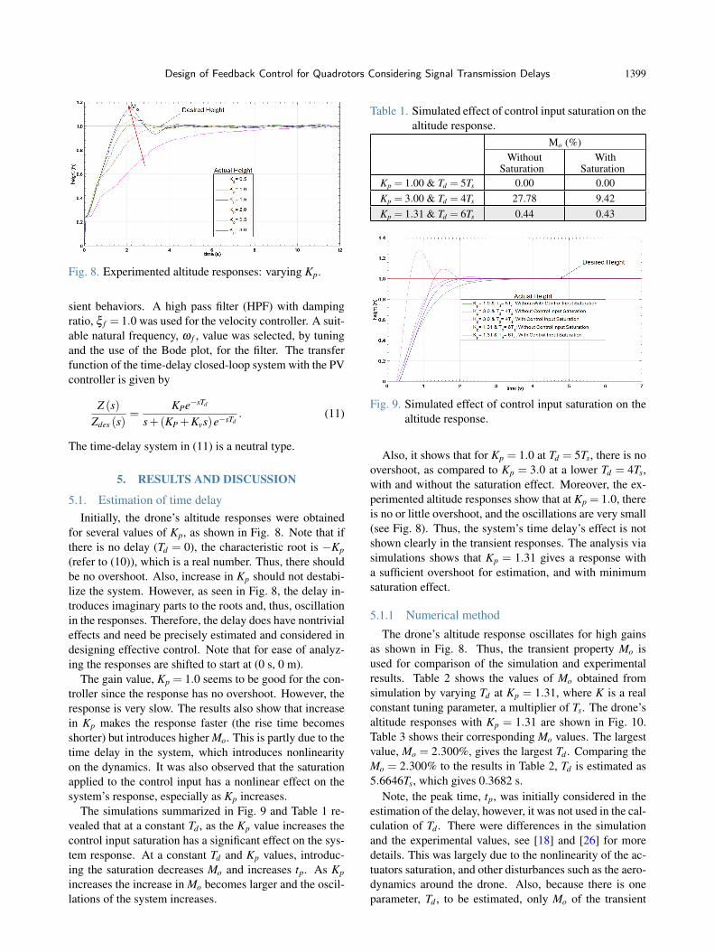
The gain value, Kp = 1.0 seems to be good for the con-troller since the response has no overshoot. However, theresponse is very slow. The results also show that increasein Kp makes the response faster (the rise time becomesshorter) but introduces higher Mo. This is partly due to thetime delay in the system, which introduces nonlinearityon the dynamics. It was also observed that the saturationapplied to the control input has a nonlinear effect on thesystem’s response, especially as Kp increases.

The simulations summarized in Fig. 9 and Table 1 re-vealed that at a constant Td , as the Kp value increases thecontrol input saturation has a significant effect on the sys-tem response. At a constant Td and Kp values, introduc-ing the saturation decreases Mo and increases tp. As Kp

increases the increase in Mo becomes larger and the oscil-lations of the system increases.

Table 1. Simulated effect of control input saturation on thealtitude response.

Mo (%)Without

SaturationWith

SaturationKp = 1.00 & Td = 5Ts 0.00 0.00Kp = 3.00 & Td = 4Ts 27.78 9.42Kp = 1.31 & Td = 6Ts 0.44 0.43

Fig. 9. Simulated effect of control input saturation on thealtitude response.

Also, it shows that for Kp = 1.0 at Td = 5Ts, there is noovershoot, as compared to Kp = 3.0 at a lower Td = 4Ts,with and without the saturation effect. Moreover, the ex-perimented altitude responses show that at Kp = 1.0, thereis no or little overshoot, and the oscillations are very small(see Fig. 8). Thus, the system’s time delay’s effect is notshown clearly in the transient responses. The analysis viasimulations shows that Kp = 1.31 gives a response witha sufficient overshoot for estimation, and with minimumsaturation effect.

5.1.1 Numerical methodThe drone’s altitude response oscillates for high gains

as shown in Fig. 8. Thus, the transient property Mo isused for comparison of the simulation and experimentalresults. Table 2 shows the values of Mo obtained fromsimulation by varying Td at Kp = 1.31, where K is a realconstant tuning parameter, a multiplier of Ts. The drone’saltitude responses with Kp = 1.31 are shown in Fig. 10.Table 3 shows their corresponding Mo values. The largestvalue, Mo = 2.300%, gives the largest Td . Comparing theMo = 2.300% to the results in Table 2, Td is estimated as5.6646Ts, which gives 0.3682 s.

Note, the peak time, tp, was initially considered in theestimation of the delay, however, it was not used in the cal-culation of Td . There were differences in the simulationand the experimental values, see [18] and [26] for moredetails. This was largely due to the nonlinearity of the ac-tuators saturation, and other disturbances such as the aero-dynamics around the drone. Also, because there is oneparameter, Td , to be estimated, only Mo of the transient

1400 Stephen K. Armah, Sun Yi, and Wonchang Choi

Table 2. Simulated altitude responses: Kp = 1.31.K Td = KTs (s) Mo (%)

4.0000 0.2600 0.0005.0000 0.3250 0.4195.6000 0.3640 2.0675.6640 0.3682 2.2985.6646* 0.3682* 2.300*5.6660 0.3683 2.3055.7000 0.3705 2.429

Table 3. Experimented altitude responses:Kp = 1.31.Flight

1 2 3 4 5Mo(%) 2.300* 2.290 2.300* 2.270 < 2

Fig. 10. Experimented altitude responses: Kp = 1.31.

Fig. 11. Plot of the dominant roots as Td increases.

properties was sufficient for the estimation.

5.1.2 Analytical approach using characteristic roots

The drone altitude response oscillates (Figs. 8 and 10).Thus, the system has complex conjugate dominant roots.Therefore, Mo is used to determine ξ . Mo = 2.300 % (seeSection 5.1.1) and, thus, ξ is obtained as 0.7684 using(8). Applying the steps described in Section 3, Td is deter-mined as 0.3598 s using the developed MATLAB programwith initial guess value of 0.3 s. See Fig. 11 for the plot ofthe dominant roots as the delay increases.

Table 4. Rightmost characteristic roots of the PV controlsystem with Kp = 2.0 and Td = 0.4 s.

Kv Rightmost Complex Roots0.0 −1.42±3.07 j0.1 −1.98±3.25 j0.3* −3.25±24.75 j0.5 −1.84±6.98 j0.7 −0.89±7.47 j

Fig. 12. PV control system characteristic roots spectrumdistribution with Kp = 2.0 and Td = 0.4 s.

5.2. PV controller: Design and implementationAs shown above, the estimated time delay using both

the numerical and the analytical methods is approximately0.4 s. A MATLAB-based software package [27] was usedto study the stability of the neutral type of time-delay sys-tems by numerically solving the characteristic equation in(11). The closed-loop system characteristic roots within aspecified region are then plotted for various Kv values.

Fig. 12 shows the spectrum distribution of the charac-teristic roots, and Table 4 shows a summary of the right-most (i.e., dominant) roots for each system. The valueKv = 0.3 yields the most suitable stable rightmost rootsamong them. The corresponding simulation altitude re-sponses for the system were also obtained for the variousKv values, see Fig. 13. It can be seen that as Kv increasesat Kp = 2.0 and Td = 0.4 s, Mo decreases and the rise timebecomes longer. At higher values of Kv, the response isoscillatory and the system becomes unstable. This is alsoobserved in Fig. 12, that as Kv increases the roots move tothe right, increasing the instability in the system. Whenthe rightmost roots are located farther from the imaginaryaxis (towards the left), the altitude responses are more sta-bilized. That is, it has reduced overshoots and faster con-vergence.

Now, based on these analyses, a controller with Kp =2.0 and Kv = 0.3 was selected as the most suitable, withclosed-loop system response transient properties of Mo =0.44 %, ts = 1.52 s, and tp = 1.76 s. Using these controllergains, the HPF was included in the simulation control sys-

Design of Feedback Control for Quadrotors Considering Signal Transmission Delays 1401

Fig. 13. Simulated PV controller altitude response withKp = 2.0, Td = 0.4 s, without HPF.

Table 5. Simulated effect of the HPF on the altitude re-sponse by varying ω f .

ω f (rads−1)5 20 38* 50 70

Mo (%) 3.19 0.64 0.32 0.38 15.09tp (s) 3.32 2.93 1.69 1.76 2.54ts (s) 4.24 2.43 1.52 1.52 NaN

Fig. 14. Simulated effect of the HPF on the altitude re-sponse by varying ω f .

tem, and its effects on the altitude transient response wasstudied for different values of ω f , see Fig. 14 and Table 5.It is observed that at smaller ω f values the response oscil-lates, and at higher values the response distorts. The os-cillations and the distortions effects were reduced by usingthe high-order solver, ode8 (Dormand-Prince).

The HPF with ω f = 38 rads−1 and ξ f = 1.0 was thenselected, with poles of −38 repeated. Now, looking at thepoles distribution of the system in Fig. 12, it is observedthat the poles of this filter is located to the left than thepoles of the PV-feedback closed-loop system. This filterwill respond faster, therefore, it will have smaller effecton the drone’s altitude transient response. Bode plot (seeFig. 15) was used to determine the filter’s cutoff frequencyas 5.68 rads−1 (0.90 Hz).

Fig. 16 and Table 6 shows the simulation altitude re-

Fig. 15. Bode plots of the PV-feedback close-loop systemwith and without the HPF.

Table 6. PV controller altitude response transient proper-ties, with Kp = 2.0 and the HPF.

Kv

0.0 0.1 0.3* 0.5 0.7Simulation (Td = 0.4 s)

Mo (%) 15.10 10.10 0.32 0.15 0.70tp (s) 1.82 1.76 1.69 3.64 4.36ts (s) 3.28 2.87 1.52 2.33 3.04

ExperimentMo (%) 8.40 5.30 2.92 0.80 0.40tp (s) 2.21 2.15 2.18 4.76 4.07ts (s) 4.00 2.67 2.86 1.99 2.48

sponses and their corresponding transient properties, withthe HPF and Kp = 2.0, for different Kv values. The resultswith Kp = 2.0 and Kv = 0.3 yields an improved transientresponse performance, which shows that the estimation ofdelay and analysis presented help. Fig. 17 and Table 6 alsoshows the experimented altitude responses and their corre-sponding transient properties, with the HPF and Kp = 2.0,for several Kv values. It demonstrates that as the Kv valueincreases Mo decreases and in general the responses be-comes slower. The PV controller performed better forKv = 0.3, 0.5, and 0.7 at Kp = 2.0.

The simulations and experiments were conductedusing the MATLAB/Simulink fixed-step solver, ode8(Dormand-Prince). The solver calculates the states duringsimulation and code generation. Investigation revealedthat the choice of a solver has a significant effect on thedrone altitude response, refer to Fig. 18, and also see [28]and [29] for more details. The HPF performance is con-strained by the type of solver used. The filter performsbetter at higher ω f when higher-order solvers are used forexperiment.

6. CONCLUSIONS

Estimation methods for the time delay in a quadro-tor type of UAV, Parrot AR.Drone 2.0, are presented and

1402 Stephen K. Armah, Sun Yi, and Wonchang Choi

Fig. 16. Simulated PV controller altitude responses withKp = 2.0 and Td = 0.4 s.

Fig. 17. Experimented PV controller altitude responseswith Kp = 2.0.

Fig. 18. Experimented effect of Simulink solvers on thePV controller altitude response.

used for altitude regulation. Using the observed maximumovershoots and locations of the characteristic roots, thetime delay was estimated as 0.4 s. For estimation of thetime delay, an appropriate P controller was used and thegain that minimizes the effect of the applied control sig-nal saturation on the system’s response was selected. Theeffects of the time delay on the drone’s altitude responsewere analyzed. The designed PV improve system perfor-mance in terms of stability and response speed than the Pcontroller.

Simulations and experiments data sets were collected

using the MATLAB/Simulink high-order solver, ode8(Dormand-Prince). Investigation through trials revealedthat selection of the solvers has significant effects on thedrone’s altitude response. The HPF performance was con-strained by the type of solver used and the filter performedbetter with the high-order solvers.

Advanced control strategies (e.g., adaptive controllersconsidering varying payloads, robust controllers for thedrone’s attitude and x-y motions) are being developed byestimating and incorporating the time delay in the con-trol systems. This problem is significantly more challeng-ing, since the equation of motions are more complex com-pared to that of the altitude motion alone. Also, nonlinearcontrol schemes (e.g., gain scheduling) can be designedtaking into account the estimated time delay. Its perfor-mance will be compared to that of the linear PV controller.Furthermore, the presented time-delay estimating meth-ods can be extended to general systems of DDEs (higherthan first order), and be applied to delay problems in net-work systems and fault detection of actuators.

REFERENCES

[1] M. Azadegan, M.T. Beheshti, and B. Tavassoli, “UsingAQM for performance improvement of networked con-trol systems,” International Journal of Control, Automa-tion and Systems, vol. 13, no. 3, pp. 764-772, 2015.

[2] M. Kchaou, F. Tadeo, M. Chaabane, and A. Toumi, “Delay-dependent robust observer-based control for discrete-timeuncertain singular systems with interval time-varying statedelay,” Int. J. Control, Automation and Systems, vol. 12,no. 1, pp. 12-22, February 2014. [click]

[3] S. Yi, W. Choi, and T. Abu-Lebdeh, “Time-delay esti-mation using the characteristic roots of delay differentialequations,” American Journal of Applied Sciences, vol. 9,no. 6, pp. 955-960, 2012.

[4] L. Belkoura, J.P. Richard, and M. Fliess, “Parameters es-timation of systems with delayed and structured entries,”Automatica, vol. 45, no. 5, pp. 1117-1125, 2009. [click]

[5] J. P. Richard, “Time-delay systems: an overview of somerecent advances and open problems,” Automatica, vol. 39,no. 10, pp. 1667-1694, 2003. [click]

[6] G. Vásárhelyi, C. Virágh, G. Somorjai, N. Tarcai, T.Szorenyi, T. Nepusz, and Vicsek, T. “Outdoor flocking andformation flight with autonomous aerial robots,” Proc. ofthe 2014 IEEE/RSJ International Conference on IntelligentRobots and Systems (IROS 2014), pp. 3866-3873, 2014.

[7] A. Ailon and S. Arogeti, “Study on the effects of time-delays on quadrotor-type helicopter dynamics,” Proc. ofthe 22nd Mediterranean Conference of Control and Au-tomation (MED), pp. 305-310, 2014.

[8] S. Torkamani and E.A. Butcher, “Delay, state, and param-eter estimation in chaotic and hyperchaotic delayed sys-tems with uncertainty and time-varying delay,” Interna-tional Journal of Dynamics and Control, vol. 1, no. 2, pp.135-163, 2013.

Design of Feedback Control for Quadrotors Considering Signal Transmission Delays 1403

[9] R. Mamat and P. J. Fleming, “Method for on-line iden-tification of a first order plus dead-time process model,”Electronics Letters, vol. 31, no. 15, pp. 1297-1298, 1995.[click]

[10] G. P. Rangaiah and P. R. Krishnaswamy, “Estimatingsecond-order dead time parameters from underdampedprocess transients,” Chemical Engineering Science, vol.51, no. 7, pp. 1149-1155, 1996. [click]

[11] S. Ahmed, B. Huang, and S. L. Shah, “Parameter and delayestimation of continuous-time models using a linear filter,”Journal of Process Control, vol. 16, no. 4, pp. 323-331,2006. [click]

[12] G.-W. Shin, Y.-J. Song, T.-B. Lee, and H.-K. Choi, “Ge-netic algorithm for identification of time delay systemsfrom step responses,” Int. J. Control, Automation and Sys-tems, vol. 5, no. 1, pp. 79-85, 2007.

[13] G. P. Rao and L. Sivakumar, “Identification of determin-istic time-lag systems,” IEEE Transactions on AutomaticControl, vol. 21, no. 4, pp. 527-529, 1976. [click]

[14] D. C. Saha and G. P. Rao, Identification of Continuous Dy-namical Systems: the Poisson moment Functional (PMF)Approach, vol. 56, Springer, 1983.

[15] R. Pintelon and L. Van Biesen, “Identification of transferfunctions with time delay and its application to cable faultlocation,” IEEE Transactions on Instrumentation and Mea-surement, vol. 39, no. 3, pp. 479-484, 1990. [click]

[16] Q.-G. Wang and Y. Zhang, “Robust identification of con-tinuous systems with dead-time from step responses,” Au-tomatica, vol. 37, no. 3, pp. 377-390, 2001. [click]

[17] S. Sagara and Z. Y. Zhao, “Numerical integration approachto on-line identification of continuous-time systems,” Au-tomatica, vol. 26, no. 1, pp. 63-74, 1990.

[18] S. Armah and S. Yi, “Altitude regulation of quadrotor typesof UAVs considering communication delays,” Proc. of theIFAC Workshop on Time Delay Systems, pp. 263-268, 2015.

[19] W. B. Randal, “Quadrotor dynamics and control Rev0.1,” All Faculty Publications, Paper 1325 from http://scholarsarchive.byu.edu/facpub/1325, 2008.

[20] P. Corke, Robotics, Vision and Control: Fundamental Al-gorithms in MATLAB, vol. 73, Springer Science & Busi-ness Media, 2011.

[21] M. H. Tanveer, S. F. Ahmed, D. Hazry, F. A. Warsi, and M.K. Joyo, “Stabilized controller design for attitude and alti-tude controlling of quad-rotor under disturbance and noisyconditions,” American Journal of Applied Sciences, vol.10, no. 8, pp. 819-831, 2013.

[22] B. Svante and L. Ljung, “A survey and comparison of time-delay estimation methods in linear systems,” Proc. of the42nd IEEE Conf. Decision and Control, pp. 2502-2507,2003.

[23] R. M. Corless, G. H. Gonnet, D. E. Hare, D. J. Jeffrey,and D. E. Knuth, “On the Lambert W function,” Advancesin Computational Mathematics, vol. 5, no. 1, pp. 329-359,1996.

[24] H. Shinozaki and T. Mori, “Robust stability analysis of lin-ear time-delay systems by Lambert W function: some ex-treme point results,” Automatica, vol. 42, no. 10, pp. 1791-1799, 2006. [click]

[25] W. J. Palm, System dynamics, 2nd ed., McGraw-Hill,Boston, 2010.

[26] S. K. Armah, Adaptive Control for Autonomous Naviga-tion of Mobile Robots Considering Time Delay and Un-certainty, Doctoral dissertation, North Carolina A&T StateUniversity, 2015.

[27] T. Vyhlídal and Z. Pavel, “QPmR-quasi-polynomial root-finder: algorithm update and examples,” Delay Systems,pp. 299-312, Springer International Publishing, 2014.[click]

[28] Mathworks, Choosing a Solver, from http://www.mathworks.com/help/optim/ug/choosing-a-solver.html,2015.

[29] L. F. Shampine, “Error estimation and control for ODEs,”Journal of Scientific Computing, vol. 25 no. 1, pp. 3-16,2005. [click]

Stephen K. Armah received his Ph.D. de-gree in Mechanical Engineering from NCA&T SU, US, in 2015. Presently, he isan Adjunct Assistant Professor at the Me-chanical Engineering Department of NCA&T SU. His current research interestsinclude adaptive and robust control forautonomous mobile robot and time-delaysystems.

Sun Yi received his Ph.D. degree in Me-chanical Engineering from the Universityof Michigan in 2009. His current researchinterests include time-delay systems, andanalysis and control of dynamic systemswith applications to mobile robots andsatellites.

Won-Chang Choi is an Associate Profes-sor of Architectural Engineering Depart-ment at Gachon University, Seongnam-si,Korea. His research interests include de-velopment and application of high perfor-mance construction materials; health mon-itoring with non-destructive method in in-frastructure; large-scale laboratory tests.