Dynamic Effects of Feedback Control Robert Stengel Robotics and Intelligent Systems MAE 345, Princeton University, 2017 Copyright 2017 by Robert Stengel. All rights reserved. For educational use only. http://www.princeton.edu/~stengel/MAE345.html • Inner, Middle, and Outer Feedback Control Loops • Step Response of Linear, Time- Invariant (LTI) Systems • Position and Rate Control • Transient and Steady-State Response to Sinusoidal Inputs 1 Outer-to-Inner-Loop Control Hierarchy • Inner Loop – Small Amplitude – Fast Response – High Bandwidth • Middle Loop – Moderate Amplitude – Medium Response – Moderate Bandwidth • Outer Loop – Large Amplitude – Slow Response – Low Bandwidth • Feedback – Error between command and feedback signal drives next inner-most loop 2
Transcript
Dynamic Effects of Feedback Control !
Robert Stengel! Robotics and Intelligent Systems MAE 345,
Princeton University, 2017
Copyright 2017 by Robert Stengel. All rights reserved. For educational use only.http://www.princeton.edu/~stengel/MAE345.html
•! Inner, Middle, and Outer Feedback Control Loops
•! Step Response of Linear, Time-Invariant (LTI) Systems
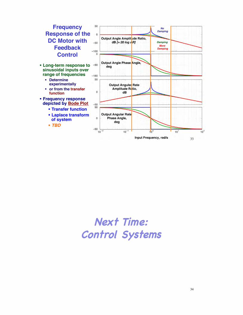
•! Position and Rate Control•! Transient and Steady-State
Response to Sinusoidal Inputs
1
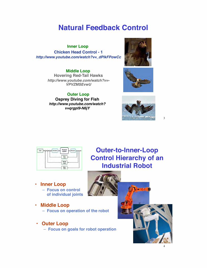
Outer-to-Inner-Loop Control Hierarchy
•! Inner Loop–! Small Amplitude–! Fast Response–! High Bandwidth
•! Middle Loop–! Moderate Amplitude–! Medium Response–! Moderate Bandwidth
•! Outer Loop–! Large Amplitude–! Slow Response–! Low Bandwidth
•! Feedback–! Error between command and
feedback signal drives next inner-most loop
2
Natural Feedback Control
Chicken Head Control - 1http://www.youtube.com/watch?v=_dPlkFPowCc
Osprey Diving for Fishhttp://www.youtube.com/watch?
... all controlled by a simple (but nonlinear) on/off switch6
Thermostat Control Logic
e(t) = yc(t)! y(t) = uc(t)! ub (t)< Thermostat >
u(t) =1(on), e(t) > 00 (off ), e(t) " 0
#$%
&%
•! Control Law [i.e., logic that drives the control variable, u(t)]
•! yc: Desired output variable (command)
•! y: Actual output•! u: Control variable
(forcing function)•! e: Control error
7
Thermostat Control Logic
•! ...but control signal would chatter with slightest change of temperature
•! Solution: Introduce lag to slow the switching cycle, e.g., hysteresis
u(t) =1 (on), e(t) ! T > 00 (off ), e(t) + T " 0
#$%
&%
u(t) =1 (on), e(t) > 00 (off ), e(t) ! 0
"#$
%$
8
Thermostat Control Logic with Hysteresis
•! Hysteresis delays the response•! System responds with a limit cycle
•!Cooling control is similar with sign reversal
9
Speed Control of Direct-Current Motor
u(t) = ce(t)where
e(t) = yc(t)! y(t)
How would y(t) be measured?
Angular Rate
Linear Feedback Control Law (c = Control Gain)
10
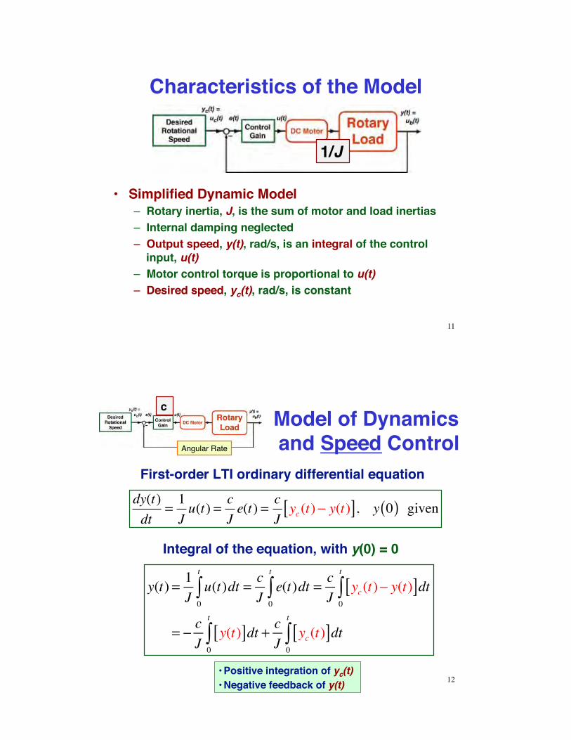
Characteristics of the Model
•! Simplified Dynamic Model–! Rotary inertia, J, is the sum of motor and load inertias–! Internal damping neglected–! Output speed, y(t), rad/s, is an integral of the control
input, u(t)–! Motor control torque is proportional to u(t) –! Desired speed, yc(t), rad/s, is constant
11
1/J
Model of Dynamics and Speed Control
First-order LTI ordinary differential equation
y(t) = 1J
u(t)dt0
t
! = cJ
e(t)dt0
t
! = cJ
yc(t)" y(t)[ ]dt0
t
!
= " cJ
y(t)[ ]dt0
t
! + cJ
yc(t)[ ]dt0
t
!
dy(t)dt
=1Ju(t) = c
Je(t) = c
Jyc (t) ! y(t)[ ], y 0( ) given
Integral of the equation, with y(0) = 0
•!Positive integration of yc(t)•!Negative feedback of y(t) 12
c
Angular Rate
Step Response of Speed Controller
y(t) = yc 1! exp!
cJ
"#$
%&' t(
)**
+
,--= yc 1! exp
.t() +, = yc 1! exp! t /(
)*+,-
•! where! !! = –c/J = eigenvalue or
root of the system (rad/sec)! "" = J/c = time constant of
the response (sec)
Step input :
yC (t) =0, t < 01, t ! 0
"#$
%$•! Solution of the integral
What does the shaft angle response look like?
13
Angular Rate
Feedback Control Lawu(t) = ce(t)where
e(t) = yc(t)! y(t)
How would y(t) be measured?
Angular Position
•! Simplified Dynamic Model–! Rotary inertia, J, is the sum of motor and load inertias–! Output angle, y(t), is a double integral of the control, u(t)–! Desired angle, yc(t), is constant