Prepared for submission to JCAP

Detecting circular polarisation in thestochastic gravitational-wavebackground from a first-ordercosmological phase transition

John Ellis,1,2,3 Malcolm Fairbairn,1 Marek Lewicki,1,4

Ville Vaskonen,1,3 Alastair Wickens1

1Department of Physics, King’s College London, Strand, WC2R 2LS London, UK2Theoretical Physics Department, CERN, Geneva, Switzerland3National Institute of Chemical Physics & Biophysics, Ravala 10, 10143 Tallinn, Estonia4Faculty of Physics, University of Warsaw ul. Pasteura 5, 02-093 Warsaw, Poland

E-mail: john.ellis@cern.ch, malcolm.fairbairn@kcl.ac.uk, marek.lewicki@kcl.ac.uk,ville.vaskonen@kcl.ac.uk, alastair.wickens@kcl.ac.uk

Abstract. We discuss the observability of circular polarisation of the stochastic gravitational-wave background (SGWB) generated by helical turbulence following a first-order cosmologicalphase transition, using a model that incorporates the effects of both direct and inverse energycascades. We explore the strength of the gravitational-wave signal and the dependence ofits polarisation on the helicity fraction, ζ∗, the strength of the transition, α, the bubble size,R∗, and the temperature, T∗, at which the transition finishes. We calculate the prospectivesignal-to-noise ratios of the SGWB strength and polarisation signals in the LISA experiment,exploring the parameter space in a way that is minimally sensitive to the underlying particlephysics model. We find that discovery of SGWB polarisation is generally more challengingthan measuring the total SGWB signal, but would be possible for appropriately strong tran-sitions with large bubble sizes and a substantial polarisation fraction.

KCL-PH-TH/2020-25, CERN-TH-2020-070

arX

iv:2

005.

0527

8v2

[as

tro-

ph.C

O]

3 S

ep 2

020

Contents

1 Introduction 1

2 Stochastic gravitational wave background from helical turbulence 32.1 Direct cascade turbulence 32.2 Inverse cascade turbulence 42.3 Sourcing GW from turbulence 6

2.3.1 Hijij(0, ω) behaviour 6

3 Spectrum of the SGWB 73.1 Stage 1 - direct cascade 8

3.1.1 Stationary approximation 83.1.2 Other models for direct cascade turbulence 8

3.2 Stage 2 - inverse cascade 103.3 GW spectrum plots 10

4 Circular polarisation of the SGWB 134.1 Computation of the polarised GW spectra 134.2 Measurements of the SGWB and its polarisation 17

5 Results for the LISA sensitivity to the SGWB and its polarisation 19

6 Conclusions 23

1 Introduction

One of the most interesting scientific targets for upcoming gravitational-wave (GW) detectorsis the stochastic gravitational-wave background (SGWB) [1, 2]. This SGWB could come frommany sources including primordial inflation [3] astrophysical sources [4] and strong phasetransitions in the early Universe [5–7].

The most easily measurable characteristic of a SGWB is its frequency spectrum, butthis provides limited insight into its origin. Further valuable information could be providedby its intrinsic circular polarisation, which is due to a difference between the amplitudes ofGWs with left and right polarisations. A SGWB generated by astrophysical sources wouldhave negligible net polarisation, since it arises from multiple uncorrelated sources. However,a cosmological SGWB could be generated coherently over large scales, and might exhibit netcircular polarisation if interactions that violate parity were important in the early Universe.Indeed, polarisation of the SGWB could in principle arise from a variety of physical mecha-nisms in the early Universe, for example gravitational chirality and modifications of gravityat high energies [8–10], pseudoscalar-like couplings between the inflaton and gauge fields [11–13] and helical turbulence created during a first-order phase transition [14, 15]. Thus thepolarisation of the SGWB could be an important diagnostic tool for probing fundamentalphysical processes in the early Universe.

With regards to the detectability of polarisation of GWs, we recall that a single linearinterferometric detector cannot probe circular polarisation in the SGWB, because it cannot

– 1 –

distinguish between left- and right-handed GWs with the same wave vector ~k. Nor can aplanar interferometer detect circular polarisation in an isotropic SGWB: it cannot distinguisha left-handed GW with a wave vector ~k from either a right-handed GW of the same amplitudeor a wave vector ~k′ that is the reflection of ~k in the plane of the interferometer. However,there is a considerable body of work on the detection of polarisation in the SGWB usingthe orbital motion of one or multiple planar GW detectors [16–21], and we note that initialconstraints on the polarisation of the SGWB have already been provided by LIGO [22].

As pointed out in Ref. [17], the isotropy of the SGWB is broken by our motion relative tothe cosmological reference frame, which induces a dipole in the SGWB. This can be detectedas a difference in the amplitudes of the GWs arriving from the ~k direction compared to thosefrom the ~k′ direction, and therefore enables a planar interferometer such as LISA to probe thepossible net circular polarisation of a SGWB. This effect was used to put a lower limit [23]on the strength of a fully-polarised constant SGWB, ΩGWh

2 ' 10−11, in order for it to bedetectable by the LISA experiment [24] or the Einstein Telescope (ET) [25].

In this work we focus on the polarisation of the SGWB that might have been generatedby helical turbulence following a first-order phase transition in the early Universe. TheStandard Model (SM) of particle physics would not have caused a first-order transition,proceeding instead via a crossover [26], but many proposed extensions of the SM would have.Examples where the SGWB from a phase transition has been studied include scenarios forbaryogenesis at the electroweak scale [27–39], models with hidden sectors [40–50], an extendedgauge group [51–58] or higher-dimensional interactions among SM fields [59, 60], and manyother models [61–84]. These examples illustrate how the SGWB may be an interesting probeof many scenarios for possible new fundamental physics beyond the SM, and a partnershipbetween GW detectors, collider and other laboratory experiments could help distinguishbetween them.

The subject of helical MHD turbulence in the primordial plasma from such a transitionhas been extensively discussed in the literature [85–88] and is often looked at in the context ofits impact on any potential primordial magnetic field [88–90]. However, more recently someeffort has been put into understanding the potential effects it could have on the period of GWgeneration expected after a first-order phase transition and whether this could be imprintedon the GW spectrum [7, 15, 91–95]. For the purpose of our work we are particularly interestedin assessing the detectability of a potential net circular polarisation of the SGWB arising fromhelical MHD turbulence following a first-order phase transition.

In order to be relatively insensitive to the details of models, we characterise them bythe helicity fraction, ζ∗, the strength of the transition, α, the average bubble size, R∗, andthe temperature, T∗, at which the transition is completed. We calculate the prospectivesignal-to-noise ratios (SNRs) of the SGWB frequency spectrum and polarisation signals forLISA.

The outline of our paper is as follows. In Section 2 we review and discuss how helicalturbulence in the primordial plasma may source polarisation in the SGWB generated duringa first-order phase transition. In Section 3 we calculate the spectrum of the SGWB, andin Section 4 we present our calculation of the possible polarisation of the SGWB. Section 5presents our results for the observability by LISA of polarisation in the SGWB as a functionof the strength of the first-order phase transition, the bubble size and the temperature atwhich the tranistion occurs, as well as the assumed initial helicity fraction. Finally, Section 6presents our conclusions.

– 2 –

2 Stochastic gravitational wave background from helical turbulence

In this section we discuss relevant aspects of the epoch following the phase transition, duringwhich we expect magnetohydrodynamic (MHD) turbulence to be generated in the primordialplasma.

The turbulent regime develops over time due to a system of eddy currents that are firstgenerated at the scale of the bubble radius, R∗, and subsequently extend over a range ofboth larger and smaller length scales. This network of eddies allows for plasma and magneticenergy, both initially concentrated at the scale R∗, to be spread throughout the MHD systemin a ‘cascade’ of energy, as discussed in [96]. Once MHD turbulence has fully developed ata given scale it decays freely, and we expect equipartition between the plasma and magneticenergy densities, ρM ∼ ρK ∼ ρeq.

As we discuss further in Section 2.2, the behaviour of the turbulence can be dramaticallychanged if the initial magnetic field left over after the phase transition has a non-zero helicalcomponent [97]. Such magnetic helicity could be generated via a variety of mechanismsincluding bubble collisions at the electroweak [98, 99] or QCD [100, 101] phase transitions,baryon-number-violating processes such as decaying non-perturbative field configurations,e.g. electroweak sphalerons [102], or even via inflation [103]. We do not discuss further thepossible origin of this helical turbulence, but parametrise it by the initial helicity fraction ofthe magnetic field left over after the transition.

2.1 Direct cascade turbulence

Collisions of bubbles at the end of the phase transition cause stirring of the primordialplasma on scales close to the average radius R∗ of the bubbles. In order to compute thecharacteristic velocity of such turbulent motions at the beginning of the turbulent period, wefirst identify two distinct forms in which the liberated vacuum energy, typically quantified byα = ρvac/ρrad, is initially deposited. We express these forms quantitatively via GW efficiencyfactors κi.

First, a fraction of the available vacuum energy goes into accelerating the bubble wall,which is expressed using the GW efficiency factor κcol. This fraction should generally besubtracted from the total energy subsequently deposited into the plasma. However, we will bedealing with transitions that are not strong enough to produce a runaway scenario, meaningthat bubble walls will reach a terminal velocity due to their friction with the surroundingplasma long before collision. Therefore, it is valid to assume that essentially all the energyis transferred to the plasma, so that αeff = α (1− κcol) ≈ α [60].

The vacuum energy deposited into the plasma can either be transferred into bulk fluidmotion that sources GWs or can be used in heating up the plasma itself. Thus, as is commonin the literature, we finally express the fraction of vacuum energy in our GW source as thefraction transferred into fluid motion [24, 60, 104]:

κsw =α

0.73 + 0.083√α+ α

, (2.1)

where we have assumed for simplicity that the speed of expansion of the walls is relativelyfast, with vw ≈ 1. We can then express the RMS fluid velocity as [96, 105]

Uf =

√3

4

α

1 + ακsw . (2.2)

– 3 –

Assuming that all the energy left in the bulk fluid motion when the flow becomes nonlinear isconverted into vortical turbulent motions of the plasma, we take κturb ≈ κsw [60] and assumethat the characteristic velocity of the plasma at the beginning of the turbulent period is asshown in Eq. (2.2).

This initial vortical fluid motion drives the formation of a hierarchy of eddy currents,first on scales around the bubble radius and subsequently on scales λ ≤ R∗. This is known asthe ‘direct energy cascade’. We parameterise the turbulent system with the quantity ξM (t),known as the magnetic correlation length which describes the maximum scale at which themagnetic field is correlated and thus physically represents the size of the largest magneticeddy. During the direct cascade period energy is transferred from the initial correlation scaleof the turbulence ξM (t∗) ' R∗, to increasingly smaller scales until it is viscously dissipatedas heat at the dissipation scale of the plasma, λd.

The distribution of magnetic and plasma energy at different scales in a direct cascadeis known to follow a Kolmogorov decay law ρ∗,i(λ, t∗) ≈ ρ∗,iλ−2/3 where i = K,M for kineticand magnetic components, respectively [93, 106]. We assume that this direct cascade periodof turbulence lasts for a few times longer than the characteristic turn-over time of the largesteddy, τ0 = R∗/Uf , so that the hierarchy of eddy currents have time to equilibrate.1 Thusthe duration of this stage of turbulence is τdirect = s0τ0, where in this paper we make therepresentative choice s0 = 3 [106].

2.2 Inverse cascade turbulence

We expect helicity to be conserved in a highly conductive plasma. Thus, if there is some initialhelicity left over in the magnetic field after the phase transition, which we parameterise withthe initial magnetic helicity fraction ζ∗ as defined in [106], we expect it to be approximatelyconserved during the direct cascade period of turbulence. After this stage the turbulence,with the plasma and the magnetic field both in equipartition, relaxes to a fully helical state,since the non-helical turbulent energy is fully dissipated away at small scales in contrast tothe conserved helical component [96].

This results in a second period of ‘inverse cascade’ turbulence following the direct cas-cade stage, during which the remaining fully helical turbulence can only be transferred toscales that are increasingly larger than the bubble radius. For large enough initial helicityfractions, this can result in a rapid increase in the magnetic correlation length of the turbu-lence, ξM (t), which corresponds physically to a large increase in the size of the largest eddy,compared with the direct cascade period.

Adopting Model B outlined in detail in [106] and originally based on the work of [107,108], we take the following evolution law for the magnetic eddy correlation scale

ξM (t) ' R∗(

1 +t

τ1

)2/3

, (2.3)

where τ1 ' R∗/v1 = τ0/ζ1/2∗ is the characteristic eddy turn-over time of the largest eddy

at the beginning of the inverse cascade stage, v1 ' ζ1/2∗ Uf is the associated characteristic

plasma velocity, and we have used the relation R∗ = τ0Uf . Furthermore, the evolution of the

1The eddy turn-over time is defined as the time it takes for an eddy at a given plasma scale to completeone full revolution.

– 4 –

magnetic and kinetic energy densities are given by

ρM (t) ' wb21

(1 +

t

τ1

)−2/3

,

ρK(t) ' wv21

(1 +

t

τ1

)−2/3

,

(2.4)

where v1 ' ζ1/2∗ Uf and b1 ' ζ1/2

∗ b0 are, respectively, characteristic velocity and magnetic fieldperturbations at the beginning of the inverse cascade stage, and v1 ' b1 due to equipartitionof the two components. The turnover time at the correlation scale of the turbulence (τ

ξ) and

the inverse cascade timescale (τinverse) then evolve as

τξ' τinverse '

ξM (t)

vk(t)= τ1

(1 +

t

τ1

), (2.5)

where we have used that vk(t) ∝ v1(1 + tτ1

)−1/3 from Eq. (2.4). Putting Eq. (2.3) togetherwith Eq. (2.5), we obtain the time when turbulence exists on the scale ξM (t) as

τinverse ' τ1

(ξM (t)

R∗

)3/2

= τ1

(k0

kξ(t)

)3/2

, (2.6)

where the wavenumber of the largest eddy is defined as kξ(t) ≡ 2π/ξM (t).Based on the approach used in [109], we compute the GW output during the inverse

cascade period by adopting a stationary turbulence model wherein, rather than consider-ing freely-decaying turbulence, we consider stationary turbulence with a duration time thatdepends on the scale, k, being considered, i.e.,

τinverse(k) ≈ τ1

(k0

k

)3/2

. (2.7)

Thus we can express the turn-over time associated with the largest scale, ks, when the inversecasade stops as

τs ≈ τ1

(k0

ks

)3/2

. (2.8)

In the absence of any effective mechanisms for dissipating the turbulence at the largest scales,an inverse cascade can cause the correlation length of the magnetic field to increase greatlyduring this period, limited only by the Hubble expansion of the universe. Thus, the inversecascade stops either at a scale, λs, when the correlation length of the turbulence reaches theHubble radius,

λs ≤ H−1∗ , (2.9)

or the inverse cascade stops after a time, τs, when the turn-over time of the largest eddyreaches the expansion timescale,

τs = τ1

(k0

ks

)3/2

=λ

3/2s

Ufζ1/2∗ R

1/2∗≤ H−1

∗ . (2.10)

Since R∗H∗, Uf and ζ∗ are all less than unity, we see that the inequality Eq. (2.10) givesa stronger condition than (2.9). Thus we obtain an expression for the scale at which theinverse cascade stops by saturating the inequality

λsR∗≤(

UfR∗H∗

)2/3

ζ1/3∗ . (2.11)

– 5 –

2.3 Sourcing GW from turbulence

We consider statistically homogeneous and isotropic turbulence, which sources GW lastingfor a limited time τT < H−1

∗ , so that the expansion of the universe may be ignored during theperiod in which the gravitational radiation is produced. Furthermore, following [106, 110], wemake the additional simplifying assumption that direct cascade MHD turbulence decaying ona time scale τdirect is equivalent to stationary turbulence with duration τdirect/2, as justifiedby the argument for unmagnetised turbulence in [111]. For the inverse cascade period wealso consider stationary turbulence [106], but this time with a scale-dependent duration timeas outlined in Section 2.2. There has been some debate in the literature [7, 110] regardingthe extent to which assuming a stationary source is a valid simplification. 2 However, whilstsuch an approximation has limitations, it is currently the only available model that hasa complete treatment of helicity and inverse cascade turbulence, and hence the potentialpolarisation signal. Thus, our results may be considered as a demonstration of principle,which may be used as a prototype for other, more sophisticated calculations. We expect thatour results will be refined as many unknowns in the simulation and modelling of turbulenceare clarified.

As shown in [110], in order to find the total GW energy density at a point in space andtime we integrate over a spherical shell centered at that point that contains all GW sourceswith a light-like distance from such an observer. The thickness of the shell would thencorrespond to the duration of the phase transition, and its radius would correspond to theproper distance between observer and source along a light-like trajectory. Following [106, 110]we can estimate the ensuing GW signal strength with ±25% accuracy by working in theaero-acoustic approximation (k→ 0). Using our premise that the source is homogeneous andisotropic and making the aforementioned simplifying assumption that the source is stationary,the integral for the total GW energy density finally simplifies to

ρGW(ω∗) =dρGW

d lnω∗= 16π3ω3

∗Gw2τTHijij(0, ω∗) , (2.12)

where ω∗ = ω(t∗) is the angular frequency measured at the time of the phase transition andw is the enthalpy density. The scalar quantity Hijij(0, ω∗) is the double trace of the four-dimensional power spectrum of the energy density tensor describing stationary turbulence inthe k→ 0 approximation [106].

2.3.1 Hijij(0, ω) behaviour

The quantity Hijij controls both the peak frequency and shape of the resulting GW signal,and its functional form varies depending on whether one is considering direct cascade orinverse cascade turbulence, as we outline in more detail below.

Stage 1 - Model for the direct cascade

In the case of direct cascade turbulence, Hijij takes the form [106]

H(stage 1)ijij (0, ω) ≈

7C2kε

6π3/2

∫ kd

k0

dk

k6exp

(− ω2

ε2/3k4/3

)erfc

(− ω

ε1/3k2/3

), (2.13)

2This debate is especially relevant in the case of direct cascade turbulence where no attempt has beenmade to account for the decay of the source by considering scale dependent turbulence, in contrast to inversecascade tubulence.

– 6 –

where ε = k0U3f = k0M

3 is the energy dissipation rate per unit enthalpy, M = Uf < 1 isthe turbulent Mach number and Ck is a constant that is O(1). We assume that in the aboveintegral k0 kd, where k0 is the wavenumber associated with the average bubble radiusthat sets the characteristic scale of the turbulence, and kd is the wavenumber associated withthe scale at which the turbulence is dissipated by viscosity. As we are considering MHDturbulence, we take the prefactor of Eq. (2.13) as 7/6, after doubling the result for purehydrodynamic turbulence given in [110] to account for approximate equipartition between themagnetic and kinetic energy components. The integral (2.13) for direct cascade turbulenceis dominated by large-scale contributions at wavenumbers close to k0, corresponding to theaverage bubble radius and, as such, we expect the GW signal for this stage of turbulence topeak at frequencies close to this scale.

Stage 2 - Model for the inverse cascade

For the period of freely-decaying inverse cascade MHD turbulence we adopt the ‘Model B’introduced in Section 2.2 and outlined in [106].3. The form of Hijij(0, ω) associated with theinverse cascade period is then expressed as

H(stage 2)ijij (0, ω) ≈ 7C2

1M3ζ

3/2∗

6π3/2k3/20

∫ k0

ks

dk

k7/2exp

(− ω2k0

ζ∗M2k3

)erfc

(− ωk

1/20

ζ1/2∗ Mk3/2

), (2.14)

where ζ∗ is the fraction of magnetic helicity left over at the end of the phase transition,and C1 is a O(1) constant that links the magnetic energy and helicity densities with theirrespective power spectra.

3 Spectrum of the SGWB

In order to calculate the spectrum of GW radiation measured today, we redshift Eq. (2.12) tonow and normalise it to the critical energy density required to make the universe flat (k = 0),namely ρc = 3H2

0/(8πG), defining the fraction of energy density in GWs today as

ΩGW,0 =

(a∗a0

)4 ρGW,∗ρc,0

=

(a∗a0

)128π4

3H20

ω3G2w2∑m=1,2

τ(stage m)T H

(stage m)ijij (0, ω∗) , (3.1)

where ω = (a∗/a0)ω∗, the enthalpy density w = 4ρ∗/3 = 2π2g∗T4∗ /45, and H2

∗ = 8πGρ∗/3 =8π3Gg∗T

4∗ /90. Rearranging this relation, we obtain G2w2 = H4

∗/4π2, and substituting this

back into the Eq. (3.1) we get

ΩGW,0 =

(a∗a0

)32π2

3H20

ω3H4∗

∑m=1,2

τ(stage m)T H

(stage m)ijij (0, ω∗)

=

(a∗a0

)1× 1037

Hz2 ω3H4∗

∑m=1,2

τ(stage m)T H

(stage m)ijij (0, ω∗) ,

(3.2)

where we have used H0 = h0 × 100 km sec−1 Mpc−1 with h0 = 0.67 [114].

3If we had used the ‘Model A’ also outlined in [106], which was originally based on the work of [112, 113],we would have found the same peak frequency but a mild suppression of the GW peak amplitude.

– 7 –

3.1 Stage 1 - direct cascade

3.1.1 Stationary approximation

After normalising Eq. (2.13), we can express the peak frequency of the GW signal due todirect cascade turbulence at the time of the transition as

fpeak,∗ = 1.48M/R∗ , (3.3)

which after red-shifting gives a peak frequency today of

fpeak,0 =a∗a0fpeak,∗ = 2.45× 10−5 Hz

(T∗

100 GeV

)(g∗

100

)1/6 M

R∗H∗, (3.4)

where we have used the relation

a∗a0≈ 8× 10−16

(100GeV

T∗

)(100

g∗

)1/3

. (3.5)

The peak amplitude of the direct cascade GW signal can then be written as

Ω(stage 1)GW,0 = 7.357× 10−6

(100

g∗

)1/3

(R∗H∗)(τTH∗

)C2kM

6 , (3.6)

where τTH∗ ≤ 1 is the duration of the Stage 1 direct cascade turbulence normalised to theHubble time, R∗H∗ is the average bubble radius at percolation normalised to the Hubbleradius, M is the Mach number and Ck is a constant of order unity.

The τTH∗ factor in Eq. (3.6) tells us that, as expected, the longer lasting the period ofdirect cascade turbulence the larger the abundance of GW emitted during this direct cascadestage. The average bubble size R∗H∗ < 1 sets the characteristic length scale of the problem,and thereby controls the peak frequency of the GW spectrum arising from direct cascadeturbulence, as seen in Eq. (3.4). A larger bubble radius R∗H∗ also implies fewer bubbles perHubble horizon, which in turn means a higher energy concentration as the bubbles convertvacuum energy from their volume into the walls. After the bubble collisions this results ina more inhomogeneous energy distribution centred around the scale R∗, and thus a higherabundance of GWs as exhibited by the factor ∝ R∗H∗ seen in (3.6).

3.1.2 Other models for direct cascade turbulence

Several other models for approximating the GW signal from direct cascade turbulence havebeen proposed in the literature. Generalising (3.3), they may be characterised by the peakfrequency at the time of the phase transition:

fpeak,∗ =A

R∗, (3.7)

which is redshifted to the following generalisation of (3.4) today,

fpeak,0 = BHzT∗

100GeV

(g∗

100

) 16 1

R∗H∗, (3.8)

where A and B are constants that depend on the way the turbulent GW source is modelled.They take the following values in some commonly-used source models:

– 8 –

• The stationary approximation discussed above yields A = 1.48M , B = 2.45× 10−5M ,and the spectra shown as black curves in Figs. 1 & 2 below;

• The top-hat approximation yields A = 5.1, B = 8.46 × 10−5 (see Eq. (85) of [7]), andthe spectra shown as dark grey curves in Figs. 1 & 2 below;

• The coherent approximation yields A = 0.586, B = 9.728× 10−6 (see Eq. (80) of [7]);

• The incoherent approximation yields A = 8.64, B = 1.43× 10−4 (see Eq. (76) of [7]).

In the LISA phase transitions working group review paper [24] the main source of GWsignal from plasma flow is associated with sound waves. The GW spectrum for this sourceis [105, 115–117]

h2Ωsw,0 = 0.9× 10−6 (R∗H∗) (τswH∗)

(κvα

1 + α

)2(100

g∗

) 13

Ssw(f) , (3.9)

where κsw is the efficiency with which vacuum energy is transformed into bulk motion of thefluid (and can be easily expressed for fast bubble walls, see Eq. (2.1)), and the spectral shapeis

Ssw(f) = (f/fsw)3

(7

4 + 3(f/fsw)2

)7/2

. (3.10)

Finally, there is an additional suppression factor that depends on fluid velocity (see Eq. (2.2))

τswH∗ = min

(1,R∗H∗Uf

), (3.11)

which is associated with the time at which shocks develop in the flow [116], and is much lessthan one for most models [59, 60, 96, 118]. The peak frequency of the sound wave source atthe time of the phase transition reads

fsw,∗ =3.38

R∗(3.12)

which becomes

fsw,0 = 5.61× 10−5 HzT∗

100GeV

(g∗

100

) 16 1

R∗H∗(3.13)

when redshifted to the present day. This contribution provides the light grey curves in Figs. 1& 2 below.

In order to model the GWs sourced from turbulence, Ref. [24] used the top-hat ap-proximation to estimate the signal for reasons outlined in [7]. Assuming Kolmogorov-typeturbulence, they calculate the associated GW spectrum arising from this model to be

h2Ωturb,0 = 1.14× 10−4 (R∗H∗)

(κswα

1 + α

) 32(

100

g∗

) 13

Sturb(f) , (3.14)

where vw is the wall velocity 4, R∗H∗ is the amplitude suppression factor discussed in theprevious section, and we have also used κsw as the efficiency for conversion of the latent heat

4We assume vw ∼ 1 in this work.

– 9 –

released during the phase transition into MHD turbulence. This comes from our optimisticassumption that when the flow becomes non-linear and the sound wave period ends, theremaining energy is readily converted into turbulence. Given that we discuss scenarios inwhich the sound wave period lasts a relatively short time, very little energy is lost and weexpect this to be a reasonable approximation. However, in principle there can be an extradamping factor due to, for example, loss of sound wave energy into reheating the plasma.The corresponding spectral shape is

Sturb(f) =(f/fturb)3

[1 + (f/fturb)]113 (1 + 8πf/h∗)

, (3.15)

where

h∗ = 16.5× 10−6 Hz

(T∗

100GeV

)(g∗

100

)1/6

(3.16)

is the inverse Hubble time at GW production redshifted to today. This contribution providesthe dark grey curves in Figs. 1 & 2 below.

3.2 Stage 2 - inverse cascade

In contrast to the direct cascade, the length scale providing the largest contribution to the

H(stage 2)ijij (0, ω) quantity used to calculate the GW signal arising from the inverse cascade

period of turbulence is model-independent, being simply set by the Hubble scale. This isbecause the majority of the turbulent energy is found around the Hubble scale at the end ofthe inverse cascade before it is dissipated due to the expansion of the universe as outlinedin Section 2.2. Taking the value of the Hubble parameter at the phase transition and red-shifting it to today, we find that the characteristic frequency of the inverse cascade GWspectrum today is

fhorizon,0 = 1.65× 10−5 Hz

(T∗

100GeV

)(g∗

100

)1/6

. (3.17)

As we will see in the examples in the next section, at this frequency the power-law of abun-dance of GWs changes from ΩGW ∝ f3 as expected beyond the horizon scale [119] to aflatter plateau composed of contributions from both the direct cascade turbulence and thehelicity fraction dependent inverse cascade turbulence. The size of the plateau depends onthe magnitude of the helicity fraction: for small ζ∗ the signal briefly levels off before revertingto its original ΩGW ∝ f3 growth rate; whilst for sufficiently large ζ∗ the plateau continues allthe way up to the scale associated with the bubble size at the transition (see Eq. (3.8)).

3.3 GW spectrum plots

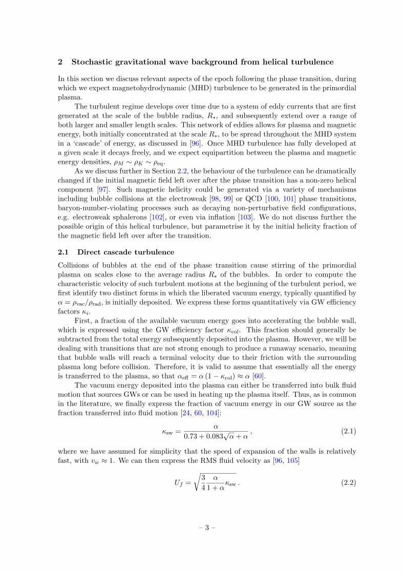
Fig. 1 and Fig. 2 compare our calculated GW spectra (black) for representative choices ofthe model parameters α,R∗ and T∗ with the LISA [24] and AEDGE [120] sensitivity curves(shown in orange and green, respectively). The value of M is not an independent quantity,being related to the magnitude of α (see Eq. (2.2)). Our calculations are for four values ofthe helicity fraction ζ∗ = 0.05 (solid), 0.1 (dashed), 0.5 (dash-dotted) and 1 (dotted).

The comparisons in Fig. 1 are for fixed T∗ = 100 GeV and different choices of theparameters α (going down) and R∗H∗ (going across), describing the strength of the first-order transition and the bubble size R∗ respectively. We recall that α sets the value of the

– 10 –

Figure 1: Our calculations of GW spectra for fixed T∗ = 100 GeV and ζ∗ = 0.05 (solid black),0.1 (dashed black), 0.5 (dash-dotted black) and 1.0 (dotted black), compared with calculationsof the spectra from sound waves (light grey) and turbulence (dark grey) taken from [24]. Thevalue of R∗H∗ increases from left to right and the value of α decreases from top to bottom.The parameter values are the same as in panel (a) unless specified. The power-law integrated(PI) LISA [24] sensitivity to the total SGWB spectrum is shown as an orange line and thePI AEDGE [120] sensitivity is shown as a green line, each for a 4-year integration time.

turbulent Mach number M through Eq. (2.2). The value of M affects the peak frequency andamplitude of the direct cascade GW signal through Eqs. (3.4) and (3.6), respectively, whilstthe characteristic amplitude of the inverse cascade GW signal is given by Eq. (2.14).

Fig. 1(a) shows that, as ζ∗ increases, the size of the low-frequency plateau in the GWspectrum arising from the inverse cascade period of turbulence, which was discussed in Sec-tion 3.2, also increases. Indeed, for large enough ζ∗ where the contribution to the GWspectrum from the inverse cascade period is sufficiently sizeable, the plateau transitions intoa distinct new peak at a frequency slightly below the frequency of the direct cascade peak.Similar features are seen in Fig. 1(b) and 1(c).

Comparing Fig. 1(a) with Fig. 1(b), we see that decreasing the value of R∗H∗ ≤ 1 bothsuppresses the amplitude of the GW signal and pushes it to higher frequencies. This is to beexpected from the analysis in Section 3.1. Furthermore, we see that the relative contributionof the low-frequency inverse cascade turbulence to the overall GW amplitude decreases withincreasing R∗H∗, because for larger values of R∗ the inverse cascade turbulence has less time

– 11 –

to develop before being washed out by the Hubble expansion.Comparing Fig. 1(a) with Fig. 1(c) where the value of α (and thus the value of M) has

been decreased, we see that for smaller values of α the peak frequency of the GW spectrumis shifted to lower frequencies and the amplitude is suppressed.

Comparing our predictions with the top-hat approximation favoured in the LISA phasetransitions working group review paper [24] (dark grey curves), we see that the peak fre-quencies are closer for larger α (and M). The heights of our peaks increase with ζ∗ and aregenerally higher than the top-hat peaks for α = 1.0, but lower for α = 0.1. Both our calcula-tions and the top-hat approximation for the choices α = 1.0 and R∗H∗ = 0.01 (Fig. 1(a)) and0.1 (Fig. 1(b)) yield spectra peaking well within the sensitivity of LISA, whereas for α = 0.1and R∗H∗ = 0.01 (Fig. 1(c)) both peaks lie below the LISA sensitivity.

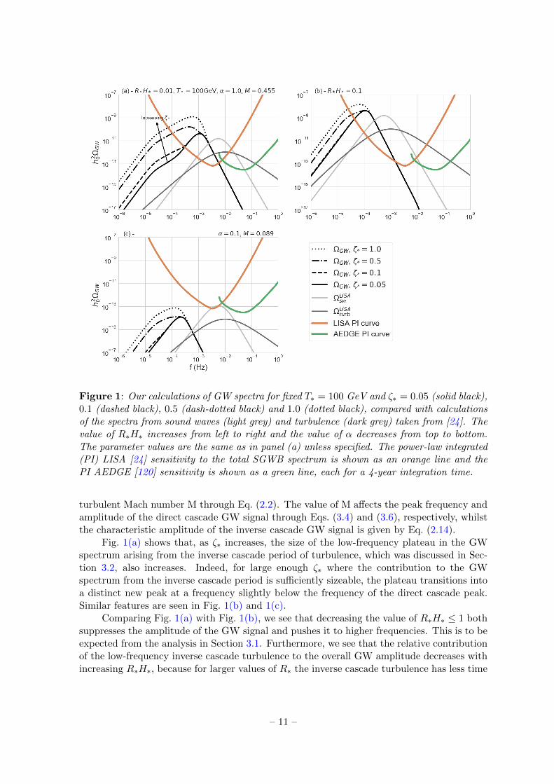
In Fig. 2 we display comparisons similar to Fig. 1, but now fixing α = 1.0 and R∗H∗ =0.01 and choosing different transition temperatures T∗. (Fig. 1(a) is repeated here as panel(c).) The peaks of the calculated spectra shift to larger frequencies for larger T∗. We cansee from Fig. 1(a) that our calculations for T∗ = 1 TeV peak within the LISA [24] sensitiv-ity, whereas the peak of the top-hat calculation peaks within the AEDGE [120] sensitivity.Fig. 1(b) shows that for T∗ = 10 TeV our peak reaches within the AEDGE sensitivity, whereasthe peak of the top-hat calculation peaks at higher frequency.

Our calculations indicate that LISA and AEDGE have complementary capabilities todetect the SGWB from a first-order phase transition, with the higher frequency range ofAEDGE extending the detectable range of T∗ to higher values.

– 12 –

Figure 2: Similar to Fig 1 but for fixed α = 1.0, R∗H∗ = 0.01 and varying T∗, whichincreases from left to right and decreases from top to bottom.

4 Circular polarisation of the SGWB

4.1 Computation of the polarised GW spectra

The circular polarisation of a GW signal is given by [14, 15]

PGW(k) =〈h+?(k)h+ (k′)− h−?(k)h− (k′)〉〈h+?(k)h+ (k′) + h−?(k)h− (k′)〉

=IA(K)

IS(K), (4.1)

where h+ and h− are the states corresponding to right- and left-handed circularly polarisedGWs, and K = k/k0 is a wavenumber normalised to the wavenumber associated with thebubble radius at collision, k0. The explicit calculation of the polarisation of the GW spectrumusing Eq. (4.2) is only required for the direct cascade period of turbulence where ζ∗ < 1. Forthe GW spectrum emitted during the inverse cascade period, on the other hand, we simplyassume that the emitted GW spectrum is fully polarised, on the premise that ζ∗ ' 1 at thebeginning of the inverse cascade stage.

In the particular case of helical turbulence the relevant functions can be approximated

– 13 –

as [15]

IS(K) '∫dP1 P1

∫dP2 P2 Θ

[(1 + γ2

p

) (1 + β2

p

)PnS1 PnS2 + 4h2γpβpP

nA1 PnA2

],

IA(K) ' 2h

∫dP1 P1

∫dP2 P2 Θ

[(1 + γ2

p

)βpP

nS1 PnA2 +

(1 + β2

p

)γpP

nA1 Pns2

],

(4.2)

where

γp =K2 + P 2

1 − P 22

2KP1, βp =

K2 + P 22 − P 2

1

2KP2,

Θ = θ (P1 + P2 −K) θ (P1 +K − P2) θ (P2 +K − P1) ,

(4.3)

and θ is the Heaviside step function. The parameter h is the fraction of helicity dissipation asdefined in [15], which is related to the magnetic helicity fraction. Indeed, these two parameterscoincide in the helical Kolmogorov turbulence model: ζ∗ ' h [15]. Following the approach in[15], which seeks to generalise the polarisation degree calculation for helical hydrodynamicturbulence given in [14] to the case of helical MHD turbulence, in this paper we determine thepolarisation degree of the direct cascade period by modelling the source as stationary5 andusing the symmetric and helical spectral indices, nS = −11/3 and nA = −14/3, consistentwith a helical Kolmogorov spectrum.6 We take the integration limits in Eq. (4.2) to rangefrom 1 to kd/k0, and simply discard scales larger than the bubble radius, i.e., k < k0, whichare only relevant to the inverse cascade period of turbulence.

Using ΩGW(k) ∝ k5〈h(k)2〉, we can rearrange Eq. (4.1) to obtain

ΩGW(k)PGW(k) = Ω+GW(k)− Ω−GW(k) , (4.4)

where ΩGW(k) = Ω+GW(k) + Ω−GW(k). Then, for the helical turbulence model we consider in

this paper, we have

Ω+GW(k) =

1 + Pstage 1GW (k)

2Ωstage 1(k) + Ωstage 2(k) ,

Ω−GW(k) =1− Pstage 1

GW (k)

2Ωstage 1(k) ,

(4.5)

where we have assumed Pstage 2GW (k) ≈ 1, on the basis that by the beginning of the second stage

ζ∗ ≈ 1 and we are in a regime of strong helical turbulence that can be well approximatedby a helicity transfer spectrum [14, 15] where PGW(k) ≈ 1 across the range of k relevant toinverse cascade turbulence. In the large wave-number limit where this approximation couldno longer hold, the contribution of Stage 2 to the GW abundance is negligible. We plot thedegree of polarisation of GWs emitted during Stage 1 direct cascade turbulence in Fig. 3.We see that Pstage 1

GW reaches a peak at K ∼ 2, whose height increases with h = ζ∗, and thenfalls for larger K.

5Debate regarding the validity of modelling the direct cascade source as stationary is of less importancewhen the helicity fraction is large given our results shown later demonstrate that in this regime the inversecascade spectrum, which attempts to account for the turbulent decay through scale dependent decorrelation,dominates the overall signal.

6If the helicity fraction is large, strong helical turbulence modelling [14] could be more appropriate, andwould result in a larger helicity fraction from the first stage of turbulence. However, as we demonstratelater and have explicitly checked for all our results, the contribution from the second stage of turbulence isalways clearly dominant in the case of a large helicity fraction, and for simplicity we use here the Kolmogorovspectrum also for the first stage.

– 14 –

0 2 4 6 8 100.0

0.2

0.4

0.6

0.8

1.0

K

PGWstage1(K

)

ζ*=1

ζ*=0.5

ζ*=0.1

HTHK

Figure 3: The degree of polarisation of Stage 1 direct cascade GWs as a function of thenormalised wavenumber K = k/k0, assuming the indicated values of the helicity dissipationparameter h. The value of h coincides with the initial magnetic helicity fraction ζ∗ for thehelical Kolmogorov turbulence (HK) model as considered in this paper, shown by solid lines.We also show with dashed lines the polarisation fraction for Stage 1 turbulence driven by theHelicity Transfer (HT) model whose use may be more appropriate in the large helicity regime.However, we find the choice of Stage 1 model has no material impact on our overall resultsin this scenario as discussed in the text.

Fig. 4 displays the strengths of the signals for different GW polarisations Ω±GW for fixedT∗ = 100 GeV, R∗H∗ = 0.01, α = 1.0, and various choices of the initial helicity fraction,ζ∗. We see in Fig. 4(a) that for small ζ∗ . 0.05 the total GW signal Ωtot

GW is dominatedby the contribution from direct cascade turbulence with negligible net polarisation, i.e.,Ω+

GW ' Ω−GW. Conversely, the small low-frequency inverse cascade plateau in the signalemits fully-polarised GW, Ω+

GW ' ΩtotGW, as expected from our previously-stated assumption

that ζ∗ ' h. Moving to Fig. 4(b), we see that raising ζ∗ to 0.1 increases the size of the fully-polarised inverse cascade plateau in the GW signal, an effect that continues until ζ∗ ∼ 0.5(Fig. 4(c)) where it begins to dominate and transitions from being a plateau into a distinctnew peak of the total GW signal. We see in the lower two panels of Fig. 4 that for ζ∗ & 0.5the contribution of the fully-polarised inverse cascade GW increasingly dominates that of thetotal GW signal, Ωtot

GW.Fig. 5 shows the Ω±GW signal strengths for fixed T∗ = 100 GeV, ζ∗ = 0.4, α = 1.0,

and various choices of R∗H∗. We can see that as R∗H∗ decreases the total GW amplitudedecreases, as expected from the discussion in the previous section. However, the net polarisa-tion of the signal increases as R∗H∗ decreases. This is because inverse cascade turbulence ismore important at smaller R∗H∗ since the turnover time of the largest eddy, τs, takes longerto reach the Hubble timescale for phase transitions with smaller average bubble radius. Thusthe duration of the inverse cascade stage where fully-polarised GWs are emitted increases,resulting in a GW signal with larger net polarisation.

Figs. 4 and 5 also feature power-law integrated sensitivities for LISA: the orange curvesare the usual PI sensitivity for the total gravitational wave signal [121], while in purple weshow PI curves for a polarisation signal. We refer the reader to Section 4.2 for a formalderivation. The interpretation is the same as in the unpolarised case, i.e., a power law witha polarisation fraction PGW (see Eq. (4.4)) crossing a purple line with the same PGW givesSNR≥ 10 for a polarisation measurement with LISA.

As can be seen in Fig. 2, the effect of increasing T∗ would be to shift the ΩGW signal to

– 15 –

Figure 4: The strengths of the polarised ΩGW,± signals for various values of the initialhelicity fraction, ζ∗ and fixed α = 1.0, T∗ = 100 GeV and R∗H∗ = 0.01. The orange curvesshow the power-law integrated sensitivity of LISA for the total GW signal, and the purple linesshow LISA’s power-law integrated sensitivity to the polarised signal assuming polarisationfractions (see Eq. (4.4)) PGW = 1, 0.1 and 0.01 as the solid, dashed and dot-dashed lines,respectively.

Figure 5: The strengths of the polarisation of the ΩGW,± signals for various values of theaverage bubble radius, R∗H∗, ζ∗ and fixed ζ∗ = 0.4 α = 1.0 and T∗ = 100 GeV. The orangeand purple sensitivity curves are the same as in Fig 4.

– 16 –

higher frequencies, without changing the relative amounts of Ω±GW or their dependences onζ∗ and R∗H∗.

4.2 Measurements of the SGWB and its polarisation

The signal-to-noise ratio (SNR) for combining two GW detector channels O and O′ is

SNROO′ =

√∫ tobs

0dt

∫dfS∗OO′(f)SOO′(f)

Pn,O(f)Pn,O′(f), (4.6)

where tobs is the total duration of the measurement and Pn,O(f) and Pn,O′(f) are the noisespectral functions in the channels O and O′. Following Ref. [23], the signal function SOO′(f)for a stochastic GW background, defined via the Fourier transform of the correlator of theGW signals passing through the O and O′ channels, can be expanded as a function of thepeculiar velocity of the solar system v = 1.23× 10−3 as

SOO′(f) =3H2

0

8π2f3

∑λ

Mλ

OO′(f) ΩλGW(f)− 4i vDλOO′(f)

[Ωλ

GW(f)− f4

dΩλGW(f)

df

]+O(v2)

,

(4.7)where λ = ±1 is the GW helicity and

MλOO′(k) = 4

∫dΩk

4πeab,λ(k)ecd,λ(−k)QabO (~k)QcdO′(−~k) ,

DλOO′(k, v) = 4i

∫dΩk

4πeab,λ(k)ecd,λ(−k)QabO (~k)QcdO′(−~k) k · v ,

(4.8)

are the monopole and dipole response functions and k ≡ |~k| = 2πf . The matrices QabO,O′(~k)contain the geometries of the detector channels, and the product of the polarisation operatorsappearing in the above expressions is given by

eab,λ(k)ecd,λ(−k) =1

4

(δac − kakc − iλεaceke

)(δbd − kbkd − iλεbdeke

). (4.9)

LISA consists of three spacecraft arranged in an equilateral triangle whose sides providethree baselines, and the combinations of pairs of these baselines form three laser interferom-eters. We denote the positions of the vertices of the triangle by ~xi and we fix the side lengthto L = 2.5 × 106 km [122]. Linear combinations of the three interferometers can be used toconstruct three detector channels: A, E and T [123]. In the following we focus on the Aand E channels, which are antisymmetric combinations of the three interferometers. The Tchannel, known as the null channel, is symmetric between the three interferometers and isrelatively insensitive to the GW signal. The noise function, assumed to be equal for the Aand E channels so that Pn,A = Pn,E ≡ Pn, is given by [124, 125] 7

Pn(f) =1

3[2 + cos (f/f0)]PIMS(f) +

4

3

[1 + cos (f/f0) + cos2 (f/f0)

]PAcc(f) , (4.10)

where f0 = 1/(2πL) = 0.019 Hz and the interferometer measurement system noise is

PIMS(f) = 3.6× 10−41 Hz−1

[1 +

(2mHz

f

)4], (4.11)

7See also the LISA Data Challenge Manual [126].

– 17 –

-

-

ℳ

λ()=ℳ

λ()

-

-

-

-

λ|

λ()|/θ

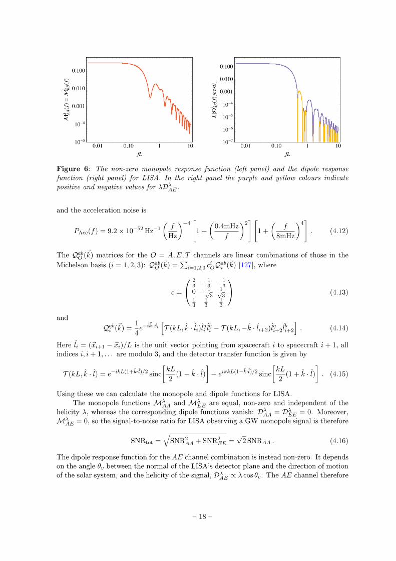
Figure 6: The non-zero monopole response function (left panel) and the dipole responsefunction (right panel) for LISA. In the right panel the purple and yellow colours indicatepositive and negative values for λDλAE.

and the acceleration noise is

PAcc(f) = 9.2× 10−52 Hz−1

(f

Hz

)−4[

1 +

(0.4mHz

f

)2][

1 +

(f

8mHz

)4]. (4.12)

The QabO (~k) matrices for the O = A,E, T channels are linear combinations of those in the

Michelson basis (i = 1, 2, 3): QabO (~k) =∑

i=1,2,3 ciOQabi (~k) [127], where

c =

23 −

13 −

13

0 − 1√3

1√3

13

13

13

(4.13)

and

Qabi (~k) =1

4e−i

~k·~xi[T (kL, k · li)lai lbi − T (kL,−k · li+2)lai+2 l

bi+2

]. (4.14)

Here li = (~xi+1 − ~xi)/L is the unit vector pointing from spacecraft i to spacecraft i + 1, allindices i, i+ 1, . . . are modulo 3, and the detector transfer function is given by

T (kL, k · l) = e−ikL(1+k·l)/2 sinc

[kL

2(1− k · l)

]+ eiπkL(1−k·l)/2 sinc

[kL

2(1 + k · l)

]. (4.15)

Using these we can calculate the monopole and dipole functions for LISA.The monopole functions Mλ

AA and MλEE are equal, non-zero and independent of the

helicity λ, whereas the corresponding dipole functions vanish: DλAA = DλEE = 0. Moreover,Mλ

AE = 0, so the signal-to-noise ratio for LISA observing a GW monopole signal is therefore

SNRtot =

√SNR2

AA + SNR2EE =

√2 SNRAA . (4.16)

The dipole response function for the AE channel combination is instead non-zero. It dependson the angle θv between the normal of the LISA’s detector plane and the direction of motionof the solar system, and the helicity of the signal, DλAE ∝ λ cos θv. The AE channel therefore

– 18 –

- -

-

-

-

-

()

(-/)

/

/

/

- -

-

-

-

-

()

Ω

=

=

=

Figure 7: Left panel: The dashed line shows the noise spectral density P1/2n for LISA, the

solid red line the corresponding sensitivity for the total GW signal and the solid purple linethe corresponding sensitivity for a fully polarised GW signal, PGW = 1. Right panel: Thepower-law integrated LISA sensitivity curves for the total GW signal and polarisation of theGW signal for a 4-year integration time with different values of the polarisation fraction PGW

(see Eq. (4.4)).

probes the circular polarisation of the GW signal and the signal-to-noise ratio for observinga circularly-polarised signal with LISA is given by

SNRpol =

√SNR2

AE + SNR2EA =

√2 SNRAE . (4.17)

The non-zero response functions MλAA =Mλ

EE and DλAE are displayed in Fig. 6.In the left panel of Fig. 7 we show the LISA sensitivities for the total GW signal and

its polarisation defined as

Ptot(f) =Pn(f)

MλAA(f)

, Ppol(f) =Pn(f)

4vDλAE(f)PGW, (4.18)

where PGW denotes the fractional polarisation of the GW signal (see Eq. (4.4)). In theright panel of Fig. 7 we show the power-law integrated sensitivity curves for LISA assumingtobs = 4 y and the threshold SNR = 10, for different values of the polarisation fractionPGW. We find that LISA can observe the polarisation of a fully-polarised GW signal downto h2

0ΩGW = 4 × 10−11, in agreement with Ref. [23]. The sensitivity scales as a function ofthe polarisation fraction of the signal as 1/PGW.

It is clear from the above discussion that detectors with just a single interferometerchannel, such as a single LIGO detector, cannot detect circular polarisation of the SGWB.Nor, indeed, can AEDGE or a pair of such detectors. On the other hand, missions withone or more triangular sets of interferometers such as ALIA, BBO [128], DECIGO [129] andAMIGO [130] would be sensitive to polarisation of the SGWB at higher frequencies thanLISA.

5 Results for the LISA sensitivity to the SGWB and its polarisation

We now assess the sensitivity of LISA to both the SGWB and to its circular polarisation,as would be generated by helical turbulence following a first-order phase transition. To do

– 19 –

this we take an approach with the least possible sensitivity to the underlying particle physicsmodel, calculating the transition strengths and temperatures, bubble sizes, and helicity frac-tions required to obtain a LISA SNR value greater than or equal to 10. This requires us todraw upon much of the analysis in the previous sections, first calculating the contributions tothe total GW spectrum (Eq. (3.2)) from both direct cascade (Eq. (2.13)) and inverse cascade(Eq. (2.14)) turbulence for a particular point in parameter space and then computing theassociated circularly-polarised spectrum (Eq. 4.5). Finally, we translate both signal typesinto the LISA SNR values associated with the total GW spectra (Eq. (4.16)) and its polarisedcounterpart (Eq. (4.17)).

The left panels of Fig. 8 display reaches in the (R∗H∗, α) plane for a LISA measurementof the overall strength of the total SGWB signal with a signal-to-noise ratio SNRtot = 10,with larger values of SNR found in the shaded regions above these lines. The panels fromtop to bottom correspond to T∗ = 10 GeV, 1 TeV and 10 TeV, and the various contourscorrespond to different values of the initial helicity fraction ζ∗. Thus, if a parameter point isenclosed within the shaded area of a given ζ∗ contour, one can infer that a GW signal withthis value of ζ∗ would be detectable by LISA with an SNR ≥ 10. The red crosses correspondto sample frequency spectra plotted in the indicated previous Figures for fixed R∗H∗, α andT∗, which exemplify the spectral sensitivity of LISA to the GW signal.

As expected, the largest detectable signals in all three panels come from larger valuesof R∗H∗, where the number of bubbles per horizon is smaller and thus the average bubbleradius at collision is larger. As R∗H∗ decreases we see that increasingly large values of thehelicity fraction, ζ∗, are required to obtain a signal with SNRtot & 10. Thus GW emissionfrom the inverse cascade turbulent period is increasingly important for LISA to be sensitiveto the total GW signal for smaller values of R∗H∗. This can be traced back to the R∗H∗suppression of the GW amplitude produced in a direct cascade that is a general feature ofthe models used to describe GW emission from turbulence (see Section 3).

We see from the different contours that increasing the initial helicity fraction increasesthe total SNR, in agreement with the increasing strength of the GW signal shown for differentvalues of ζ∗ in Fig. 1. In general, the GW signal should be detectable at a level of SNRtot & 10for α & 1 and R∗H∗ & 10−3 for a transition at T∗ = 100 GeV. For larger values of T∗, largervalues of R∗H∗ are needed for SNRtot = 10 measurements, though smaller values of α aresufficient.

We also see in the left panels of Fig. 8 that for large values of R∗H∗ the position of theSNRtot = 10 contours are approximately independent of ζ∗ and depend only on α, whereasfor smaller values of R∗H∗ the contour lines have a greater dependence on the value of ζ∗associated with the contour. This is explained by the fact that for large R∗H∗ the contributionof inverse cascade period is minimised as the large average bubble radius at collision meansinverse cascade turbulence cannot operate for very long before being washed out by theHubble expansion. Thus increasing ζ∗ does relatively little to increase the amplitude ofthe signal (see Fig. 1(b)) and has minimal effect on its sensitivity to LISA. Conversely, forsmall R∗H∗ the inverse cascade can operate for far longer before being washed out by theexpansion, and thus the potential contribution from the inverse cascade to the total GWsignal can be much larger (see Fig. 1(a)). As larger values of ζ∗ result in greater importanceof the inverse cascade period for the total GW signal, it follows that in the low-R∗H∗ region

– 20 –

of the parameter space, the SNRtot is much more sensitive to the value of ζ∗8.

The right panels of Fig. 8 display the corresponding reaches in the (R∗H∗, α) plane for aLISA measurement of the circular polarisation of the SGWB with SNRpol = 10. As expectedthe reach is smaller than for the total GW signal, but we see that many of the qualitativefeatures of the plots of SNRtot described above are also present in the polarised case. Whilstdetection prospects for circular polarisation in the SGWB are strongest for large R∗H∗ wherethe suppression in the amplitude of the spectra is minimised (see Fig. 5), in order for LISA tobe able to probe a circularly-polarised signal at small R∗H∗, larger values of ζ∗ are requiredto compensate for the suppression R∗H∗ introduces into the total GW signal. Larger ζ∗means fully-polarised GWs from the inverse cascade period make an increasingly importantcontribution to the total GW signal, raising the amplitude of Ω+

GW relative to Ω−GW andincreasing the prospects for detection by LISA of circular polarisation in the SGWB from aphase transition.

Comparing the right panels of Fig. 8, we see that for smaller values of the helicityfraction, ζ∗ . 0.2, LISA is most sensitive to polarisation of the GW signal when the transitiontemperature is T∗ = 1 TeV. This can be understood by looking at Fig. 2 and noting that, ofthe three transition temperatures, the T∗ = 1 TeV spectrum peaks at the optimal frequencyto be sensitive to the fully-polarised low-frequency inverse cascade plateau that develops inthe signal for small ζ∗.

As seen in the right hand panels of Fig. 8, in the polarised case the positions of theSNRpol = 10 contours exhibit a larger relative dependence on ζ∗ at large R∗H∗ than theirSNRtot counterparts. Whilst in the Ωtot

GW case the low-frequency inverse cascade contributionwas less important for larger R∗H∗, in the polarised case it has a larger impact. Even whenconsidering the case of a low-frequency plateau in the signal associated with relatively lowhelicity inverse cascade turbulence (see see Fig. 4(a)), fully-polarised GW are still beingemitted, implying that relatively small changes in the value of ζ∗ can have a larger effect onthe net polarisation of the SGWB and the ability of LISA to probe it.

As seen in the top right panel of Fig. 8, for larger values of the helicity fraction, ζ∗ & 0.3,the parameter space in which SNRpol > 10 expands significantly in the T∗ = 100GeV case,allowing a larger range of small R∗H∗ values to be probed by LISA. This can be understoodby referring to the T∗ = 100GeV spectrum plot in Fig. 1(a) and noting that for intermediatevalues of the helicity fraction, 0.1 . ζ∗ . 0.5 the low-frequency, fully-polarised inverse cascadeplateau transitions into a new, distinct peak, and in so doing becomes rapidly more sensitiveto the frequency band where LISA is most sensitive.

Similar behaviour is seen for the T∗ = 1 TeV case shown in the middle panel of Fig. 8,though less pronounced, because the GW spectra for this transition temperature peak athigher frequencies where LISA is already more sensitive to the fully-polarised inverse cascadeplateau.

8We note that new simulations suggest that the f1 plateau at low frequencies could also develop in caseswith small initial helicity [95]. This would improve detection prospects for low-ζ∗ scenarios and reduce thedependence of the total SNR on that parameter.

– 21 –

Total signal Polarised signal

Figure 8: Signal-to-noise (SNR) = 10 contours in the (R∗H∗, α) plane for T∗ = 100 GeV(top), T∗ = 1 TeV (middle) and T∗ = 10 TeV (bottom), for a LISA measurement with a4-year observation time. In the left panels the SNR is shown for the total SGWB signaland in the right panels for observing the polarisation of the SGWB. The different contourscorrespond to various values of the initial helicity fraction ζ∗, as shown in the plots. The redcrosses correspond to sample GW spectra for fixed α, R∗H∗ and T∗ plotted in the indicatedprevious Figures, which allow comparison of the LISA sensitivity to the GW signal for rangesof ζ∗ values.

– 22 –

6 Conclusions

We have analysed in this paper the prospects for detection of circular polarisation of thestochastic GW background produced by a first-order phase transition at a temperature T∗ ≥100 GeV. We focused on an analytical model for the sourcing of GWs by MHD turbulenceproduced in the plasma during the transition. Crucially, the model allows us to describe notonly a direct energy cascade in the plasma but also an inverse cascade that develops if thereis some initial helicity fraction in the fluid motion, usually sourced from helicity left over inthe magnetic field after the transition. The direct cascade describes energy transferred intosmaller scales, and the resulting signal peak corresponds to the characteristic scale of thetransition, which is related to the average bubble size R∗.

If some initial helicity fraction is present in the plasma, then the helical component ofthe energy in the MHD turbulence will be conserved during the direct cascade, whilst thenon-helical part will be dissipated away at small scales due to the plasma’s intrinsic viscosity.This results in a period of inverse cascade MHD turbulence following the direct cascade,where the turbulence is fully helical and energy in the turbulence is instead transferred toincreasingly large scales. This process lasts for the rest of the Hubble time, and continuouslyproduces a GW signal forming a plateau in wavelength that extends to the horizon size.Critically, the signal produced during this second stage of the turbulence will be circularlypolarised and, provided the initial helicity fraction is large enough, it results in an overallstochastic background with a significant degree of polarisation.

We have compared our results with the more common description of fluid dynamicsinvolving a sound wave period followed by a top-hat approximation to the turbulence. Thecrucial difference between the models is the characteristic scale, which depends in the modelwe use not only on the bubble size but also the Mach number. This induces a dependenceon the average fluid velocity which becomes lower in weaker transitions, causing the GWspectrum to peak at lower frequencies.

We have revisited the capability of future GW detectors to measure the polarisation of aSGWB background, focusing on LISA. We find that in the model we use to describe the signalarising from MHD turbulence following a phase transition, detection with SNRpol > 10 couldbe possible. However, this would require a sufficiently strong phase transition with α ' 1 aswell as either a large helicity fraction close to unity or large bubbles of sizes approaching thehorizon size. The smaller the helicity fraction, the more supercooled the transition wouldhave to be to produce an observable polarisation in the stochastic GW background signal.

We conclude that LISA may have a significant opportunity to measure polarisation of theSGWB. However, we emphasise several caveats. The strength of any such signal is sensitiveto the strength of the underlying first-order phase transition and the sizes of the bubbles itproduces. In particular, potentially observable signals would require a significant amount ofsupercooling, potentially leading to new difficulties in modeling the turbulence not yet takeninto account. Moreover, the chances of such a measurement depend crucially on the seedingof some helical turbulence in the primordial plasma. We emphasise also that the modelwe have used to calculate the amount of polarisation certainly requires improvement, andshould be tensioned against other models as they emerge. We look forward to improvementsin understanding any possible cosmological first-order phase transition and the possible originand magnitude of helical turbulence, and improvements in modelling their consequences.

– 23 –

Acknowledgements

The work of JE, MF, ML and VV was supported by the United Kingdom STFC GrantST/P000258/1. Also, JE received support from the Estonian Research Council grant MOBTT5,ML was partly supported by the Polish National Science Center grant 2018/31/D/ST2/02048,and would also like to acknowledge hospitality and support from KITP at UCSB, where partof this work was carried out, supported in part by the National Science Foundation underGrant No. NSF PHY-1748958. MF and AW were funded by the European Research Councilunder the European Union’s Horizon 2020 programme (ERC Grant Agreement no.648680DARKHORIZONS), and VV was partly supported by the Estonian Research Council grantPRG803. ML, VV and AW would also like to express gratitude to the organizers of theGravitational Waves from the Early Universe programme at NORDITA for providing a greatworking environment from which this project benefited, as well as partial support during theprogramme.

References

[1] B. Allen, The Stochastic gravity wave background: Sources and detection, in Relativisticgravitation and gravitational radiation. Proceedings, School of Physics, Les Houches, France,September 26-October 6, 1995, pp. 373–417, 1996. gr-qc/9604033.

[2] C. Caprini and D. G. Figueroa, Cosmological Backgrounds of Gravitational Waves, Class.Quant. Grav. 35 (2018) 163001, [1801.04268].

[3] N. Bartolo et al., Science with the space-based interferometer LISA. IV: Probing inflation withgravitational waves, JCAP 12 (2016) 026, [1610.06481].

[4] T. Regimbau, The astrophysical gravitational wave stochastic background, Res. Astron.Astrophys. 11 (2011) 369–390, [1101.2762].

[5] E. Witten, Cosmic Separation of Phases, Phys. Rev. D30 (1984) 272–285.

[6] M. S. Turner and L. M. Widrow, Inflation Produced, Large Scale Magnetic Fields, Phys. Rev.D37 (1988) 2743.

[7] C. Caprini, R. Durrer and G. Servant, The stochastic gravitational wave background fromturbulence and magnetic fields generated by a first-order phase transition, JCAP 0912 (2009)024, [0909.0622].

[8] C. R. Contaldi, J. Magueijo and L. Smolin, Anomalous CMB polarization and gravitationalchirality, Phys. Rev. Lett. 101 (2008) 141101, [0806.3082].

[9] N. Bartolo and G. Orlando, Parity breaking signatures from a Chern-Simons coupling duringinflation: the case of non-Gaussian gravitational waves, JCAP 07 (2017) 034, [1706.04627].

[10] S. Alexander and N. Yunes, Chern-Simons Modified General Relativity, Phys. Rept. 480(2009) 1–55, [0907.2562].

[11] N. Barnaby, E. Pajer and M. Peloso, Gauge Field Production in Axion Inflation:Consequences for Monodromy, non-Gaussianity in the CMB, and Gravitational Waves atInterferometers, Phys. Rev. D 85 (2012) 023525, [1110.3327].

[12] P. Adshead, E. Martinec and M. Wyman, Perturbations in Chromo-Natural Inflation, JHEP09 (2013) 087, [1305.2930].

[13] E. Dimastrogiovanni, M. Fasiello and T. Fujita, Primordial Gravitational Waves fromAxion-Gauge Fields Dynamics, JCAP 01 (2017) 019, [1608.04216].

– 24 –

[14] T. Kahniashvili, G. Gogoberidze and B. Ratra, Polarized cosmological gravitational wavesfrom primordial helical turbulence, Phys. Rev. Lett. 95 (2005) 151301, [astro-ph/0505628].

[15] L. Kisslinger and T. Kahniashvili, Polarized Gravitational Waves from Cosmological PhaseTransitions, Phys. Rev. D92 (2015) 043006, [1505.03680].

[16] N. Seto, Quest for circular polarization of gravitational wave background and orbits of laserinterferometers in space, Phys. Rev. D 75 (2007) 061302, [astro-ph/0609633].

[17] N. Seto, Prospects for direct detection of circular polarization of gravitational-wavebackground, Phys. Rev. Lett. 97 (2006) 151101, [astro-ph/0609504].

[18] N. Seto and A. Taruya, Measuring a Parity Violation Signature in the Early Universe viaGround-based Laser Interferometers, Phys. Rev. Lett. 99 (2007) 121101, [0707.0535].

[19] N. Seto and A. Taruya, Polarization analysis of gravitational-wave backgrounds from thecorrelation signals of ground-based interferometers: Measuring a circular-polarization mode,Phys. Rev. D 77 (2008) 103001, [0801.4185].

[20] J. D. Romano and N. J. Cornish, Detection methods for stochastic gravitational-wavebackgrounds: a unified treatment, Living Rev. Rel. 20 (2017) 2, [1608.06889].

[21] T. L. Smith and R. Caldwell, Sensitivity to a Frequency-Dependent Circular Polarization inan Isotropic Stochastic Gravitational Wave Background, Phys. Rev. D 95 (2017) 044036,[1609.05901].

[22] S. Crowder, R. Namba, V. Mandic, S. Mukohyama and M. Peloso, Measurement of ParityViolation in the Early Universe using Gravitational-wave Detectors, Phys. Lett. B 726 (2013)66–71, [1212.4165].

[23] V. Domcke, J. Garcia-Bellido, M. Peloso, M. Pieroni, A. Ricciardone, L. Sorbo et al.,Measuring the net circular polarization of the stochastic gravitational wave background withinterferometers, JCAP 05 (2020) 028, [1910.08052].

[24] C. Caprini et al., Science with the space-based interferometer eLISA. II: Gravitational wavesfrom cosmological phase transitions, JCAP 1604 (2016) 001, [1512.06239].

[25] B. Sathyaprakash et al., Scientific Objectives of Einstein Telescope, Class. Quant. Grav. 29(2012) 124013, [1206.0331].

[26] K. Kajantie, M. Laine, K. Rummukainen and M. E. Shaposhnikov, Is there a hot electroweakphase transition at m(H) larger or equal to m(W)?, Phys. Rev. Lett. 77 (1996) 2887–2890,[hep-ph/9605288].

[27] J. M. No, Large Gravitational Wave Background Signals in Electroweak BaryogenesisScenarios, Phys. Rev. D 84 (2011) 124025, [1103.2159].

[28] F. P. Huang, Y. Wan, D.-G. Wang, Y.-F. Cai and X. Zhang, Hearing the echoes of electroweakbaryogenesis with gravitational wave detectors, Phys. Rev. D 94 (2016) 041702, [1601.01640].

[29] M. Chala, G. Nardini and I. Sobolev, Unified explanation for dark matter and electroweakbaryogenesis with direct detection and gravitational wave signatures, Phys. Rev. D94 (2016)055006, [1605.08663].

[30] A. Katz and A. Riotto, Baryogenesis and Gravitational Waves from Runaway BubbleCollisions, JCAP 11 (2016) 011, [1608.00583].

[31] V. Vaskonen, Electroweak baryogenesis and gravitational waves from a real scalar singlet,Phys. Rev. D95 (2017) 123515, [1611.02073].

[32] G. C. Dorsch, S. J. Huber, T. Konstandin and J. M. No, A Second Higgs Doublet in the EarlyUniverse: Baryogenesis and Gravitational Waves, JCAP 1705 (2017) 052, [1611.05874].

– 25 –

[33] M. Artymowski, M. Lewicki and J. D. Wells, Gravitational wave and collider implications ofelectroweak baryogenesis aided by non-standard cosmology, JHEP 03 (2017) 066,[1609.07143].

[34] A. Beniwal, M. Lewicki, J. D. Wells, M. White and A. G. Williams, Gravitational wave,collider and dark matter signals from a scalar singlet electroweak baryogenesis, JHEP 08(2017) 108, [1702.06124].

[35] F. P. Huang and C. S. Li, Probing the baryogenesis and dark matter relaxed in phasetransition by gravitational waves and colliders, Phys. Rev. D 96 (2017) 095028, [1709.09691].

[36] A. Beniwal, M. Lewicki, M. White and A. G. Williams, Gravitational waves and electroweakbaryogenesis in a global study of the extended scalar singlet model, JHEP 02 (2019) 183,[1810.02380].

[37] S. Bruggisser, B. Von Harling, O. Matsedonskyi and G. Servant, Electroweak Phase Transitionand Baryogenesis in Composite Higgs Models, JHEP 12 (2018) 099, [1804.07314].

[38] F. P. Huang, Z. Qian and M. Zhang, Exploring dynamical CP violation induced baryogenesisby gravitational waves and colliders, Phys. Rev. D 98 (2018) 015014, [1804.06813].

[39] S. A. R. Ellis, S. Ipek and G. White, Electroweak Baryogenesis from Temperature-VaryingCouplings, JHEP 08 (2019) 002, [1905.11994].

[40] J. R. Espinosa, T. Konstandin, J. M. No and M. Quiros, Some Cosmological Implications ofHidden Sectors, Phys. Rev. D78 (2008) 123528, [0809.3215].

[41] P. Schwaller, Gravitational Waves from a Dark Phase Transition, Phys. Rev. Lett. 115 (2015)181101, [1504.07263].

[42] J. Jaeckel, V. V. Khoze and M. Spannowsky, Hearing the signal of dark sectors withgravitational wave detectors, Phys. Rev. D94 (2016) 103519, [1602.03901].

[43] F. P. Huang and X. Zhang, Probing the gauge symmetry breaking of the early universe in 3-3-1models and beyond by gravitational waves, Phys. Lett. B 788 (2019) 288–294, [1701.04338].

[44] K. Tsumura, M. Yamada and Y. Yamaguchi, Gravitational wave from dark sector with darkpion, JCAP 07 (2017) 044, [1704.00219].

[45] I. Baldes and C. Garcia-Cely, Strong gravitational radiation from a simple dark matter model,JHEP 05 (2019) 190, [1809.01198].

[46] D. Croon, T. E. Gonzalo and G. White, Gravitational Waves from a Pati-Salam PhaseTransition, JHEP 02 (2019) 083, [1812.02747].

[47] M. Breitbach, J. Kopp, E. Madge, T. Opferkuch and P. Schwaller, Dark, Cold, and Noisy:Constraining Secluded Hidden Sectors with Gravitational Waves, JCAP 07 (2019) 007,[1811.11175].

[48] D. Croon, V. Sanz and G. White, Model Discrimination in Gravitational Wave spectra fromDark Phase Transitions, JHEP 08 (2018) 203, [1806.02332].

[49] M. Fairbairn, E. Hardy and A. Wickens, Hearing without seeing: gravitational waves from hotand cold hidden sectors, JHEP 07 (2019) 044, [1901.11038].

[50] A. J. Helmboldt, J. Kubo and S. van der Woude, Observational prospects for gravitationalwaves from hidden or dark chiral phase transitions, Phys. Rev. D100 (2019) 055025,[1904.07891].

[51] S. J. Huber, T. Konstandin, G. Nardini and I. Rues, Detectable Gravitational Waves fromVery Strong Phase Transitions in the General NMSSM, JCAP 03 (2016) 036, [1512.06357].

[52] R. Jinno and M. Takimoto, Probing a classically conformal B-L model with gravitationalwaves, Phys. Rev. D 95 (2017) 015020, [1604.05035].

– 26 –

[53] S. Iso, P. D. Serpico and K. Shimada, QCD-Electroweak First-Order Phase Transition in aSupercooled Universe, Phys. Rev. Lett. 119 (2017) 141301, [1704.04955].

[54] S. Demidov, D. Gorbunov and D. Kirpichnikov, Gravitational waves from phase transition insplit NMSSM, Phys. Lett. B 779 (2018) 191–194, [1712.00087].

[55] K. Hashino, M. Kakizaki, S. Kanemura, P. Ko and T. Matsui, Gravitational waves from firstorder electroweak phase transition in models with the U(1)X gauge symmetry, JHEP 06(2018) 088, [1802.02947].

[56] C. Marzo, L. Marzola and V. Vaskonen, Phase transition and vacuum stability in theclassically conformal B–L model, Eur. Phys. J. C 79 (2019) 601, [1811.11169].

[57] K. Miura, H. Ohki, S. Otani and K. Yamawaki, Gravitational Waves from WalkingTechnicolor, JHEP 10 (2019) 194, [1811.05670].

[58] A. Azatov, D. Barducci and F. Sgarlata, Gravitational traces of broken gauge symmetries,1910.01124.

[59] J. Ellis, M. Lewicki and J. M. No, On the Maximal Strength of a First-Order ElectroweakPhase Transition and its Gravitational Wave Signal, JCAP 1904 (2019) 003, [1809.08242].

[60] J. Ellis, M. Lewicki, J. M. No and V. Vaskonen, Gravitational wave energy budget in stronglysupercooled phase transitions, JCAP 1906 (2019) 024, [1903.09642].

[61] G. C. Dorsch, S. J. Huber and J. M. No, Cosmological Signatures of a UV-ConformalStandard Model, Phys. Rev. Lett. 113 (2014) 121801, [1403.5583].

[62] M. Kakizaki, S. Kanemura and T. Matsui, Gravitational waves as a probe of extended scalarsectors with the first order electroweak phase transition, Phys. Rev. D 92 (2015) 115007,[1509.08394].

[63] K. Hashino, M. Kakizaki, S. Kanemura, P. Ko and T. Matsui, Gravitational waves and Higgsboson couplings for exploring first order phase transition in the model with a singlet scalarfield, Phys. Lett. B766 (2017) 49–54, [1609.00297].

[64] P. Huang, A. J. Long and L.-T. Wang, Probing the Electroweak Phase Transition with HiggsFactories and Gravitational Waves, Phys. Rev. D 94 (2016) 075008, [1608.06619].

[65] J. Kubo and M. Yamada, Scale genesis and gravitational wave in a classically scale invariantextension of the standard model, JCAP 12 (2016) 001, [1610.02241].

[66] C. Balazs, A. Fowlie, A. Mazumdar and G. White, Gravitational waves at aLIGO and vacuumstability with a scalar singlet extension of the Standard Model, Phys. Rev. D 95 (2017)043505, [1611.01617].

[67] I. Baldes, Gravitational waves from the asymmetric-dark-matter generating phase transition,JCAP 05 (2017) 028, [1702.02117].

[68] L. Marzola, A. Racioppi and V. Vaskonen, Phase transition and gravitational wavephenomenology of scalar conformal extensions of the Standard Model, Eur. Phys. J. C77(2017) 484, [1704.01034].

[69] Z. Kang, P. Ko and T. Matsui, Strong first order EWPT & strong gravitational waves inZ3-symmetric singlet scalar extension, JHEP 02 (2018) 115, [1706.09721].

[70] F. P. Huang and J.-H. Yu, Exploring inert dark matter blind spots with gravitational wavesignatures, Phys. Rev. D 98 (2018) 095022, [1704.04201].

[71] M. Chala, C. Krause and G. Nardini, Signals of the electroweak phase transition at collidersand gravitational wave observatories, JHEP 07 (2018) 062, [1802.02168].

[72] E. Megias, G. Nardini and M. Quiros, Cosmological Phase Transitions in Warped Space:Gravitational Waves and Collider Signatures, JHEP 09 (2018) 095, [1806.04877].

– 27 –

[73] T. Prokopec, J. Rezacek and B. Swiezewska, Gravitational waves from conformal symmetrybreaking, JCAP 1902 (2019) 009, [1809.11129].

[74] V. Brdar, A. J. Helmboldt and J. Kubo, Gravitational Waves from First-Order PhaseTransitions: LIGO as a Window to Unexplored Seesaw Scales, JCAP 1902 (2019) 021,[1810.12306].

[75] M. Chala, M. Ramos and M. Spannowsky, Gravitational wave and collider probes of a tripletHiggs sector with a low cutoff, Eur. Phys. J. C79 (2019) 156, [1812.01901].

[76] P. Baratella, A. Pomarol and F. Rompineve, The Supercooled Universe, JHEP 03 (2019) 100,[1812.06996].

[77] A. Angelescu and P. Huang, Multistep Strongly First Order Phase Transitions from NewFermions at the TeV Scale, Phys. Rev. D99 (2019) 055023, [1812.08293].

[78] A. Alves, T. Ghosh, H.-K. Guo, K. Sinha and D. Vagie, Collider and Gravitational WaveComplementarity in Exploring the Singlet Extension of the Standard Model, JHEP 04 (2019)052, [1812.09333].

[79] P. S. B. Dev, F. Ferrer, Y. Zhang and Y. Zhang, Gravitational Waves from First-Order PhaseTransition in a Simple Axion-Like Particle Model, JCAP 1911 (2019) 006, [1905.00891].

[80] R. Jinno, H. Seong, M. Takimoto and C. M. Um, Gravitational waves from first-order phasetransitions: Ultra-supercooled transitions and the fate of relativistic shocks, JCAP 1910(2019) 033, [1905.00899].

[81] X. Wang, F. P. Huang and X. Zhang, Gravitational wave and collider signals in complextwo-Higgs doublet model with dynamical CP-violation at finite temperature, Phys. Rev. D 101(2020) 015015, [1909.02978].

[82] L. Delle Rose, G. Panico, M. Redi and A. Tesi, Gravitational Waves from Supercool Axions,JHEP 04 (2020) 025, [1912.06139].

[83] B. Von Harling, A. Pomarol, O. Pujolas and F. Rompineve, Peccei-Quinn Phase Transition atLIGO, JHEP 04 (2020) 195, [1912.07587].

[84] X. Wang, F. P. Huang and X. Zhang, Phase transition dynamics and gravitational wavespectra of strong first-order phase transition in supercooled universe, 2003.08892.

[85] G. Sigl, A. V. Olinto and K. Jedamzik, Primordial magnetic fields from cosmological firstorder phase transitions, Phys. Rev. D55 (1997) 4582–4590, [astro-ph/9610201].

[86] T. Kahniashvili, A. G. Tevzadze and B. Ratra, Phase Transition Generated CosmologicalMagnetic Field at Large Scales, Astrophys. J. 726 (2011) 78, [0907.0197].

[87] T. Kahniashvili, A. G. Tevzadze, A. Brandenburg and A. Neronov, Evolution of PrimordialMagnetic Fields from Phase Transitions, Phys. Rev. D87 (2013) 083007, [1212.0596].

[88] J. Ellis, M. Fairbairn, M. Lewicki, V. Vaskonen and A. Wickens, Intergalactic Magnetic Fieldsfrom First-Order Phase Transitions, JCAP 09 (2019) 019, [1907.04315].

[89] T. Kahniashvili, A. Brandenburg, L. Campanelli, B. Ratra and A. G. Tevzadze, Evolution ofinflation-generated magnetic field through phase transitions, Phys. Rev. D 86 (2012) 103005,[1206.2428].

[90] T. Kahniashvili, A. Brandenburg and A. G. Tevzadze, The evolution of primordial magneticfield since its generation, Phys. Scripta 91 (2016) 104008, [1507.00510].

[91] A. Nicolis, Relic gravitational waves from colliding bubbles and cosmic turbulence, Class.Quant. Grav. 21 (2004) L27, [gr-qc/0303084].

[92] C. Caprini and R. Durrer, Gravitational waves from stochastic relativistic sources: Primordialturbulence and magnetic fields, Phys. Rev. D 74 (2006) 063521, [astro-ph/0603476].

– 28 –

[93] T. Kahniashvili, L. Kisslinger and T. Stevens, Gravitational Radiation Generated by MagneticFields in Cosmological Phase Transitions, Phys. Rev. D 81 (2010) 023004, [0905.0643].

[94] P. Niksa, M. Schlederer and G. Sigl, Gravitational Waves produced by Compressible MHDTurbulence from Cosmological Phase Transitions, Class. Quant. Grav. 35 (2018) 144001,[1803.02271].

[95] A. R. Pol, S. Mandal, A. Brandenburg, T. Kahniashvili and A. Kosowsky, NumericalSimulations of Gravitational Waves from Early-Universe Turbulence, 1903.08585.

[96] J. Ellis, M. Lewicki and J. M. No, Gravitational waves from first-order cosmological phasetransitions: lifetime of the sound wave source, 2003.07360.

[97] J. M. Cornwall, Speculations on primordial magnetic helicity, Phys. Rev. D56 (1997)6146–6154, [hep-th/9704022].

[98] T. Stevens, M. B. Johnson, L. S. Kisslinger, E. M. Henley, W.-Y. P. Hwang and M. Burkardt,Role of Charged Gauge Fields in Generating Magnetic Seed Fields in Bubble Collisions duringthe Cosmological Electroweak Phase Transition, Phys. Rev. D 77 (2008) 023501, [0707.1346].

[99] T. Stevens and M. B. Johnson, Magnetic Seed Field Generation from Electroweak BubbleCollisions, with Bubble Walls of Finite Thickness, Phys. Rev. D 80 (2009) 083011,[0903.2227].

[100] M. M. Forbes and A. R. Zhitnitsky, Primordial galactic magnetic fields from domain walls atthe QCD phase transition, Phys. Rev. Lett. 85 (2000) 5268–5271, [hep-ph/0004051].

[101] L. S. Kisslinger, Magnetic wall from chiral phase transition and CMBR correlations, Phys.Rev. D 68 (2003) 043516, [hep-ph/0212206].

[102] C. J. Copi, F. Ferrer, T. Vachaspati and A. Achucarro, Helical Magnetic Fields fromSphaleron Decay and Baryogenesis, Phys. Rev. Lett. 101 (2008) 171302, [0801.3653].

[103] L. Campanelli, Helical Magnetic Fields from Inflation, Int. J. Mod. Phys. D 18 (2009)1395–1411, [0805.0575].

[104] J. R. Espinosa, T. Konstandin, J. M. No and G. Servant, Energy Budget of CosmologicalFirst-order Phase Transitions, JCAP 1006 (2010) 028, [1004.4187].

[105] M. Hindmarsh, S. J. Huber, K. Rummukainen and D. J. Weir, Numerical simulations ofacoustically generated gravitational waves at a first order phase transition, Phys. Rev. D 92(2015) 123009, [1504.03291].

[106] T. Kahniashvili, L. Campanelli, G. Gogoberidze, Y. Maravin and B. Ratra, GravitationalRadiation from Primordial Helical Inverse Cascade MHD Turbulence, Phys. Rev. D78 (2008)123006, [0809.1899].

[107] R. Banerjee and K. Jedamzik, Are cluster magnetic fields primordial?, Phys. Rev. Lett. 91(2003) 251301, [astro-ph/0306211].

[108] L. Campanelli, Evolution of Magnetic Fields in Freely Decaying MagnetohydrodynamicTurbulence, Phys. Rev. Lett. 98 (2007) 251302, [0705.2308].

[109] T. Kahniashvili, G. Gogoberidze and B. Ratra, Gravitational Radiation from PrimordialHelical MHD Turbulence, Phys. Rev. Lett. 100 (2008) 231301, [0802.3524].

[110] G. Gogoberidze, T. Kahniashvili and A. Kosowsky, The Spectrum of Gravitational Radiationfrom Primordial Turbulence, Phys. Rev. D76 (2007) 083002, [0705.1733].

[111] I. Proudman, The generation of noise by isotropic turbulence, Proc. R. Soc. London A 214(1952) 119–132.

[112] D. Biskamp and W.-C. Muller, Decay laws for three-dimensional magnetohydrodynamicturbulence, Phys. Rev. Lett. 83 (1999) 2195–2198.

– 29 –

[113] M. Christensson, M. Hindmarsh and A. Brandenburg, Inverse cascade in decayingthree-dimensional magnetohydrodynamic turbulence, Phys. Rev. E 64 (2001) 056405.

[114] Planck collaboration, N. Aghanim et al., Planck 2018 results. VI. Cosmological parameters,1807.06209.

[115] M. Hindmarsh and M. Hijazi, Gravitational waves from first order cosmological phasetransitions in the Sound Shell Model, JCAP 12 (2019) 062, [1909.10040].

[116] M. Hindmarsh, S. J. Huber, K. Rummukainen and D. J. Weir, Shape of the acousticgravitational wave power spectrum from a first order phase transition, Phys. Rev. D 96 (2017)103520, [1704.05871].

[117] M. Hindmarsh, Sound shell model for acoustic gravitational wave production at a first-orderphase transition in the early Universe, Phys. Rev. Lett. 120 (2018) 071301, [1608.04735].

[118] C. Caprini et al., Detecting gravitational waves from cosmological phase transitions withLISA: an update, JCAP 03 (2020) 024, [1910.13125].

[119] R.-G. Cai, S. Pi and M. Sasaki, Universal infrared scaling of gravitational wave backgroundspectra, 1909.13728.

[120] AEDGE collaboration, Y. A. El-Neaj et al., AEDGE: Atomic Experiment for Dark Matterand Gravity Exploration in Space, EPJ Quant. Technol. 7 (2020) 6, [1908.00802].

[121] E. Thrane and J. D. Romano, Sensitivity curves for searches for gravitational-wavebackgrounds, Phys. Rev. D88 (2013) 124032, [1310.5300].

[122] LISA collaboration, P. Amaro-Seoane et al., Laser Interferometer Space Antenna,1702.00786.

[123] M. R. Adams and N. J. Cornish, Discriminating between a Stochastic Gravitational WaveBackground and Instrument Noise, Phys. Rev. D 82 (2010) 022002, [1002.1291].

[124] N. J. Cornish, Detecting a stochastic gravitational wave background with the LaserInterferometer Space Antenna, Phys. Rev. D 65 (2002) 022004, [gr-qc/0106058].

[125] T. Robson, N. J. Cornish and C. Liu, The construction and use of LISA sensitivity curves,Class. Quant. Grav. 36 (2019) 105011, [1803.01944].

[126] LISA collaboration, “LISA Data Challenge Manual.”https://lisa-ldc.lal.in2p3.fr/static/data/pdf/LDC-manual-001.pdf, 2018.

[127] N. Bartolo, V. Domcke, D. G. Figueroa, J. Garcıa-Bellido, M. Peloso, M. Pieroni et al.,Probing non-Gaussian Stochastic Gravitational Wave Backgrounds with LISA, JCAP 11(2018) 034, [1806.02819].

[128] J. Crowder and N. J. Cornish, Beyond LISA: Exploring future gravitational wave missions,Phys. Rev. D 72 (2005) 083005, [gr-qc/0506015].

[129] S. Kawamura et al., Space gravitational-wave antennas DECIGO and B-DECIGO, Int. J.Mod. Phys. D 28 (2019) 1845001.

[130] W.-T. Ni, G. Wang and A.-M. Wu, Astrodynamical middle-frequency interferometricgravitational wave observatory AMIGO: Mission concept and orbit design, 1909.04995.

– 30 –