Detection and Location of Faults in Wide Area Systems ...

Graduate Theses, Dissertations, and Problem Reports

2015

Detection and Location of Faults in Wide Area Systems based on Detection and Location of Faults in Wide Area Systems based on

Error-Dependent Communication Strategy Error-Dependent Communication Strategy

Preethi Priya Vallapu

Follow this and additional works at: https://researchrepository.wvu.edu/etd

Recommended Citation Recommended Citation Vallapu, Preethi Priya, "Detection and Location of Faults in Wide Area Systems based on Error-Dependent Communication Strategy" (2015). Graduate Theses, Dissertations, and Problem Reports. 6862. https://researchrepository.wvu.edu/etd/6862

This Thesis is protected by copyright and/or related rights. It has been brought to you by the The Research Repository @ WVU with permission from the rights-holder(s). You are free to use this Thesis in any way that is permitted by the copyright and related rights legislation that applies to your use. For other uses you must obtain permission from the rights-holder(s) directly, unless additional rights are indicated by a Creative Commons license in the record and/ or on the work itself. This Thesis has been accepted for inclusion in WVU Graduate Theses, Dissertations, and Problem Reports collection by an authorized administrator of The Research Repository @ WVU. For more information, please contact [email protected].

https://researchrepository.wvu.edu/

https://researchrepository.wvu.edu/

https://researchrepository.wvu.edu/etd

https://researchrepository.wvu.edu/etd?utm_source=researchrepository.wvu.edu%2Fetd%2F6862&utm_medium=PDF&utm_campaign=PDFCoverPages

https://researchrepository.wvu.edu/etd/6862?utm_source=researchrepository.wvu.edu%2Fetd%2F6862&utm_medium=PDF&utm_campaign=PDFCoverPages

mailto:[email protected]

Detection and Location of Faults in Wide Area Systems

based on Error-Dependent Communication Strategy


Thesis submitted to the

Benjamin M. Statler College of Engineering and Mineral Resources

at West Virginia University

in partial fulfillment of the requirements for the degree of

Master of Science

in

Electrical Engineering

Dr. Parviz Famouri, Ph.D., Chair

Dr. Muhammad A. Choudhry, Ph.D.

Dr. Yaser P. Fallah, Ph.D.

Dr. Sarika Kushalani Solanki, Ph.D.

Lane Department of Computer Science and Electrical Engineering

Morgantown, West Virginia

2015

Keywords: Communication Strategy, Fault Location, Phasor measurement unit,

linear state estimation, Wide Area Measurement and Protection system.

Copyright 2015 Preethi Priya Vallapu

ABSTRACT

Detection and Location of Faults in Wide Area Systems based on

Error-Dependent Communication Strategy


Transmission system serves as a crucial link between generating stations and consumers.

Early detection and accurate location of faults on transmission lines are essential to prevent the

occurrence of blackouts. Also real time monitoring of power system states during faults will

enhance the situational awareness for power system operators. Wide Area Measurement and

Protection Systems (WAMPS) based on Phasor Measurement Unit (PMU) are a promising

solution for dynamic real time monitoring and protection of power system.

This thesis deals with detection and location of faults on a transmission system based on

synchrophasor technology. Performance of WAMPS is largely dependent on the performance of

its information and communication technologies infrastructure. Error-dependent communication

strategy is employed in this work for communication of real time data from PMU to the centralized

controller. As PMUs are expensive, they cannot be placed at every bus. Hence linear state estimator

based on synchronized measurements is employed for estimating the state of the entire system.

The estimated states of the system are then compared to a certain threshold and if any abnormality

is found, fault is detected. Once the faulted bus is detected, two-terminal algorithm is employed to

identify the exact location of fault. The proposed methodology is implemented on IEEE 9 bus

system developed in MATLAB/SIMULINK environment.

iii

ACKNOWLEDGEMENTS

Firstly, I would like to express my deepest gratitude towards my research advisor Dr. Parviz

Famouri, for all the support and encouragement he has given to me throughout my research. I

would like to acknowledge Dr. Yaser P. Fallah for all the guidance and suggestions he provided

me during the work. I am also grateful to Dr. Muhammad A. Choudhry and Dr. Sarika Kushalani

Solanki for being a part of my committee and also for providing their valuable feedback.

I would like to thank all my friends for their constant support and encouragement. Lastly, I would

like to thank my beloved parents and siblings for their unconditional love and support throughout

my life.

iv

TABLE OF CONTENTS

1. Introduction ...............................................................................................................................1

1.1 Background ......................................................................................................................................... 1

1.2 Wide Area Measurement and Protection system (WAMPS) .............................................................. 2

1.3 Linear State Estimation ....................................................................................................................... 3

1.4 Detection and Location of Faults on Wide Area System..................................................................... 5

1.5 Research Objective ............................................................................................................................. 7

1.6 Thesis Outline ...................................................................................................................................... 8

2. Wide Area Measurement and Protection system (WAMPS) .........................................................9

2.1 Introduction ........................................................................................................................................ 9

2.2 Wide Area Measurement System ....................................................................................................... 9

2.3 Phasor Measurement Unit (PMU) .................................................................................................... 11

2.3.1 Phasor Representation ............................................................................................................... 11

2.3.2 Architecture of Phasor Measurement Unit ............................................................................... 13

2.4 Communication Network .................................................................................................................. 14

2.4.1 Error-Dependent Communication Strategy ............................................................................... 16

3. Linear State Estimation ............................................................................................................. 22

3.1 Traditional State Estimation ............................................................................................................. 22

3.1.1 Component Modelling ............................................................................................................... 23

3.1.2 The Bus-Admittance Matrix ....................................................................................................... 25

3.1.3 Maximum Likelihood Estimation ............................................................................................... 26

3.1.4 Weighted Least Squares State Estimation ................................................................................. 27

3.2 Linear State Estimation ..................................................................................................................... 33

4. Detection and Location of Faults on Wide Area System ............................................................. 36

4.1 Fault Detection .................................................................................................................................. 36

4.1.1 Procedure for Fault Detection ................................................................................................... 37

4.2 Fault Location .................................................................................................................................... 40

4.2.1 Fault Location Methodology ...................................................................................................... 42

5. Simulations and Results ............................................................................................................ 45

v

5.1 Test System ....................................................................................................................................... 45

5.2 Simulation of Phasor Measurement Unit (PMU) .............................................................................. 47

5.2.1 Communication Strategy ........................................................................................................... 49

5.3 State Estimation Results based on Linear Estimator ........................................................................ 51

5.4 Fault Analysis .................................................................................................................................... 52

6. Conclusion and Future Work ..................................................................................................... 62

6.1 Conclusion ......................................................................................................................................... 62

6.2 Future Work ...................................................................................................................................... 63

7. Bibliography ............................................................................................................................. 64

vi

LIST OF FIGURES

Fig. 2.1: Layers and Components of WAMP system [13] ..................................................................... 10

Fig. 2.2: Basic architecture of WAMP system [14] ................................................................................ 11

Fig. 2.3: Phasor representation of a sinusoidal signal............................................................................ 12

Fig. 2.4: Block Diagram of PMU ............................................................................................................. 14

Fig. 2.5: Schematic overview of periodic polling strategy [12] ............................................................. 17

Fig. 2.6: Block diagram of procedure for Error-Dependent Communication Strategy [12] ............. 18

Fig. 3.1: Flow chart of Traditional State Estimator ............................................................................... 23

Fig. 3.2: Two-port model of a transmission line ..................................................................................... 24

Fig. 3.3: Transformer branch model ....................................................................................................... 24

Fig. 3.4: Tap-changing transformer ........................................................................................................ 25

Fig. 3.5: Two-port π equivalent model of transmission line ................................................................. 29

Fig. 3.6 π section model of a transmission line ....................................................................................... 34

Fig. 4.1: Matlab/Simulink block diagram developed to indicate the bus nearest to the fault location

.................................................................................................................................................................... 39

Fig. 4.2: Matlab/Simulink block diagram developed for indication of faulted line ............................ 40

Fig. 4.3: Schematic of synchronized two-ended fault location [54] ...................................................... 41

Fig. 4.4: Schematic for fault location on schematic line [54] ................................................................. 42

Fig. 4.5: Faulted transmission line [56]. .................................................................................................. 43

Fig. 4.6: Flow chart for detection and location of faults in wide area system. .................................... 44

Fig. 5.1: IEEE 9 bus test system [60] ....................................................................................................... 46

Fig. 5.2: Block diagram of PMU developed in Simulink ....................................................................... 47

Fig. 5.3: (a) 3phase analog input voltage signal, (b) Output signal obtained from PMU i.e. positive

sequence phasor voltage magnitude (p.u.) and (c) angle (degrees) ....................................................... 48

Fig. 5.4: Implemetation of Error-Dependent commnuication strategy where (a) Original signal at

sender, (b) Transmitted samples, (c)Reconstructed signal at receiver................................................. 50

Fig. 5.5: Block diagram of IEEE 9 bus system developed in Simulink ................................................ 53

Fig. 5.6: Fault Monitoring based on Error-Dependent Communication strategy .............................. 54

Fig. 5.7: Performance of Error-Dependent Communication strategy for different Error Threshold

eth values where (a) eth=0.001, (b) eth=0.01, (c) eth=0.05, (d) eth=0.1 ............................................... 55

Fig. 5.8: Comparison between Actual voltage value and estimated voltage state during fault at bus

8. ................................................................................................................................................................. 57

Fig. 5.9: Comparison between Actual voltage angle and estimated voltage angle during fault at bus

8. ................................................................................................................................................................. 57

Fig. 5.10: Comparison of estimated voltage magnitudes of all the buses for fault detection ............. 58

Fig. 5.11: Comparison of positive sequence current angle absolute difference of all the lines

connected to bus 8 ..................................................................................................................................... 59

vii

LIST OF TABLES

Table. 1: Base case Load Flow ................................................................................................................. 46

Table. 2: Comparison of Actual Voltage values obtained from load flow and the Estimated Voltage

states of the system .................................................................................................................................... 51

Table. 3: Comparison of actual voltage angles values obtained from load flow and the estimated

voltage angles of the system...................................................................................................................... 52

Table. 4: Transmission line (7-8) parameters ......................................................................................... 52

Table. 5: Accuracy of error-dependent strategy for different threshold errors ................................. 56

Table. 6: Location of Faults on Transmission Line ............................................................................... 60

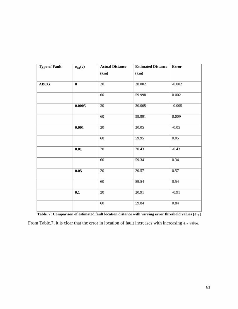
Table. 7: Comparison of estimated fault location distance with varying error threshold values (𝐞𝐭𝐡)

.................................................................................................................................................................... 61

1

1. Introduction

1.1 Background

Electrical Power Systems are one of the critical components of the modern society. The

phenomenal increase of our dependence and demand on electricity in recent times has led to

serious strain in terms of production and expansion of transmission capacity. This demand led to

the increase in the length of transmission line. Also transmission lines travel through harsh terrains

and thus monitoring and protection of large interconnected power systems has become a challenge.

As a most catastrophic result, power system large-scale blackouts, as the one that occurred on Aug

14, 2003 [1], can interrupt the power supply for a few hours, affecting millions of people and

causing huge economic loss. Analysis of the August 14, 2003 blackout in the Northeastern US has

shown that the problems developed hours before the system collapse. If the power system operators

were aware of the overall worsening system conditions that were developing, certain actions could

have been taken to avoid the blackout and restore the system. Thus power system designers need

tools for monitoring, protection and control against these Blackouts.

Modern information and communication technologies are being developed for various

aspects of power system monitoring, protection and control. For decades, traditional power system

operation and control has been performed by supervisory control and data acquisition (SCADA)

and energy management system (EMS). These measurements are taken once every 4 to 10 secs

providing steady state view of power system. However with changing portfolio of generation,

increasing loads and interconnections of national grids, real time monitoring and dynamic control

is required. To meet these requirements, one of the recently developed technologies, Wide Area

Measurement and Protection Systems (WAMPS) based on Phasor Measurement Unit (PMU) are

being deployed internationally. PMUs provide phasor measurements that are synchronized to

common reference time using high precision global positioning system (GPS) satellite. This

functionality provides dynamic real-time observation of the power system states and enables to

manage the system at a more efficient and responsive level.

PMUs were first introduced in early 1980’s and since then many applications of PMUs

have been developed around the world [2]. Synchro phasors can provide positive sequence voltage

and current phasors from anywhere on a power system which can be integrated with Phasor Data

2

Concentrators (PDC) at substations in hierarchical structure [3], [4]. Data obtained from PMU

helps to analyze sequence of events that have contributed to the catastrophic failure of power

system. PMUs are being increasingly used for detecting faults on the transmission line [5]. This

thesis deals with utilizing PMU measurements for detection and location of faults in a

Transmission system.

1.2 Wide Area Measurement and Protection system (WAMPS)

WAMP systems are a promising solution for real time monitoring and protection of power

system. Such system allows greater utilization of the transmission capacity in existing

infrastructure and fast corrective responses in abnormal transient situations in the power system.

Performance of WAMP system is largely dependent on the performance of modern information

and communication technologies infrastructure. The extensive integration of power system and its

communication infrastructure necessitates that both the systems are studied as single distributed

cyber-physical energy system (CPES). PMUs are often installed in substations which are

geographically far away from the control center PDC. Expensive and dedicated communication

networks are needed to bring synchro phasors from far locations to a centralized location. Network

bandwidth requirement increases linearly with the number of installed PMUs and also with the

increasing synchrophasor reporting rates.

The IEEE standard C37.1l8 [6] specifies the PMU output file structures, supported

reporting rates, and various other communication standards required by Synchro phasors. The data

requirements and communication latency for various applications using WAMPS is summarized

in [7]. According to [7] for monitoring and protection application minimum data required is of the

order of 100 bytes per second and maximum communication latency allowed is 50 msec.

Many recent efforts on co-simulation of power system dynamic simulator and network

simulator using an accurate synchronization mechanism have been reported in literature [8] [9]

[10]. In [8] authors presented a method to implement network simulator in OPNET and then

feeding the OPNET simulation trace into the power system mode. In [9] methods like EPOCHS

which use federation and ADEVS that require its own modeling of the continuous dynamics of

power system in DEVS frame work. An improved method using both the methods EPOCHS and

ADEVS is presented in [10]. In [11] the power system and communication network dynamics are

3

embedded into a single power system simulation environment, PSCAD. Coupling of the both

simulators is critical particularly at transient level and performance of such communication has

significant effect on the control of power system. Thus it’s important to consider control-aware

communication strategies for utilizing available communication technologies. In this work Error-

Dependent communication strategy [12] is used for sending PMU measurements to the remote

centralized controller. In this mode, communication is initiated only when there is abnormal

change in the system state. Thus in this way communication delays and failures can be reduced to

a greater extent and overall performance can be increased.

1.3 Linear State Estimation

In order to accurately monitor the power systems, many electrical quantities of the network

should be measured. This requires a significant amount of investment, which is not economically

efficient and control systems will be vulnerable to measurement errors or failures. Therefore,

various state estimation methods have been proposed in the past to determine the optimal

estimation of the system states, including unmeasured parameters based on the system models and

other measurements in the network. Most of the traditional state estimators considered steady state

system model whose measurements were available through SCADA system [19-22]. The

measurements are sent via local remote terminal units (RTUs) to the centralized control center,

which monitors and controls the entire system. The new state model of the system obtained is used

for various applications like contingency analysis, economic dispatch, unit commitment etc.

Therefore, state estimation plays a crucial role in maintaining a healthy power system. The

geographic spread and complexity of electric power system has imposed several restrictions in

implementation of power system state estimation. Measurements from multiple different locations

(substations) have to travel significant distances to the data collection and processing center,

usually referred to as energy management system (EMS). Thus communication and latencies play

an important role in determining the accuracy of the measurements. Also if the measurements are

not time stamped in a unified way, irrespective of measurement location, they can introduce

significant biases in the estimation, and may even be practically useless in a dynamic estimation

framework. Such complications have limited the power system to basic, static level state

estimation.

4

It can be summarized as the power system state estimation, in its current status, is not

capable of capturing the system dynamic behavior. It can only provide monitoring information in

the form of a sequence of steady states. This also limits the wide area control actions on the system

to very slow steady state control that is usually manually executed by the system operators. Such

control application can be, e.g. economic generation dispatch among units, power flow redirection,

reactive power and voltage profile control, static security assessment and control, load forecasting.

Fast automatic control during faults and transients in general is provided only locally, on a

component basis, not taking thus into consideration the wide area system behavior.

Rapid growth of Phasor Measurement Units (PMUs) has opened doors for dynamic state

estimation. PMUs provide synchronized measurements which are synchronized via GPS clock.

The phasors computed via a time reference, at one location, are globally valid and can be used in

local computations (making their results also globally valid) or along with data collected or

computed at different locations. So, this eliminates problems originating from the wide geographic

separation of a power system by making local measurements or computed quantities globally valid.

Several researchers have suggested ways to include phasor measurements into existing non-linear

state estimator [23] [24]. In [25] a hybrid state estimator is proposed which uses conventional

measurements as well as phasors by converting phasor measurements from polar to rectangular

form. An alternative approach to include phasor measurements in state estimation is described in

[26]. The hybrid state estimators take the advantage of accuracy of PMU measurements, which in

turn improves the overall accuracy of the estimator. However, in such hybrid state estimators the

real time reporting rate of PMU measurements is not exploited as estimator not only depends on

PMU measurements but also on conventional measurements whose reporting rate is much slower

than PMU measurements. An updated real time hybrid state estimator proposed in [27] uses

interpolation techniques for the buses that are not observed by PMUs. Although the proposed

estimator could estimate the states accurately during transient conditions, estimation of power

system state for non-observable buses was not accurate enough.

With growing number of PMU installations, state estimators that utilize only PMU

measurements, thus resulting in linear estimators, have been proposed. The first linear estimator

using PMU technology was introduced in 1994 [28]. Multi-level linear estimators have also been

proposed in [29] [30]. By using only PMU measurements for state estimation the accuracy is highly

5

improved. Another advantage is that the introduction of PMUs has made it possible to locally

measure both magnitude and phase of electrical quantities and distribute the state estimation

procedure. The main criteria for using only PMU measurements in estimation is that the system

has to be observable. As PMUs are costly devices, optimal placement of PMUs is essential.

Although optimal placement of PMU is not covered in this thesis, PMUs are placed on few buses

such as the system would be observable. The state of the remaining buses is estimated using linear

state estimator.

1.4 Detection and Location of Faults on Wide Area System

The greatest threat to power systems is system faults which could occur at any voltage

level. The majority of short-circuit faults, typically 80-90%; tend to occur on overhead

transmission lines and the rest on substation equipment and bus bars combined. Thus, detection

and location of faults on transmission line are of vital importance.

In power systems, the type of fault can be categorized as either a permanent fault or a

temporary fault. A permanent fault caused by events, such as a broken transmission line or the

malfunction of a power generator, can be located easily, as the detection devices receive huge

differences in signal characteristics during the pre-fault and post-fault moment. In contrast, the

temporary fault that is normally caused by insulator flashover would not cause the supply of the

overhead transmission to collapse immediately. However, flashover on insulators has the potential

to lead to a full breakdown of the insulator when those transient phenomena occur frequently.

Therefore, it is vital to protect and analyze the whole network and localize the fault in advance.

Also, accurate location of fault on a transmission line can expedite the repair of the fault

components, speed up restoration, reduce outage time, and, thus, improve power system reliability.

In recent years, major efforts have been dedicated to the exploration and development of

new methodologies that detect faults that occur in the overhead transmission line. Phasor

measurement units as a wide-area measurement system can also act as a wide-area protection

system on large power systems. The real time data obtained from PMUs can be used to detect the

buses nearest to the fault and consequently the faulted line is detected [40]. Various fault location

algorithms have been developed and presented in the literature. They can be classified mainly into

two types. First one is based on traveling-wave phenomenon which makes use of high-frequency

6

components of currents and voltages generated by faults [41] [42]. In travelling wave method, an

electrical pulse is sent along the transmission line. The time of the pulse return back indicates the

distance to fault point. Main disadvantage of this method is that the propagation can be

significantly affected by system parameters and network configuration. The other method is based

on an impedance principle, making use of the fundamental frequency voltages and currents [43].

This method is widely used because of its simplicity and low cost to be adapted to electronic

devices in the substations. Further, this method can be classified into two types based on number

of measurements i.e. one terminal method [43] [44] and multi-terminal method [45-48]. One-

terminal algorithms only use one terminal’s voltage and the current of the fault line. However, the

accuracy of these one-terminal algorithms may be adversely affected by the fault resistance and

the remote terminal system’s impedance. Multi terminal algorithms can be ether 2 terminal [45]

[46] or 3 terminal [47] or even more terminals [48] [49]. These multi-terminal methods are less

influenced by the fault resistance and remote terminal system’s impedance, and are theoretically

more accurate.

Although existing multi-terminal algorithms can achieve high accuracy in locating faults,

they are limited to a fault location in a transmission network where phasor measurement units

(PMUs) are installed with at least one terminal for every line. Practically, PMUs cannot be installed

with such density on transmission networks due to its high cost. In such cases state estimation can

be performed for estimating the unknown measurements so that multi terminal algorithms can be

used for fault location.

In the past use of state estimation for fault detection and location has been proposed in few

publications. For the offline fault location, [50] proposes to first compute a state estimation on the

whole network using phasor measurements. The faulted line is identified using bad data analysis.

Then, the state vector is extended to identify the fault parameters (i.e. fault resistance and distance)

at the same time as the node voltages. Because the estimation is then nonlinear, iterations are

needed for the extended state estimation and convergence of the algorithm is not guaranteed. The

disadvantage of this approach is that to identify the faulted line, a current measurement must be

present on each line segment of the network. Another approach consists in identifying the fault

parameters together with the node voltages for the fault detection and location. This was for

instance done for fault identification in DC systems in [51]. But the measurement redundancy must

7

be high enough to make the system observable and the optimization problem can be nonlinear,

which can bring convergence problems or a long computation time, which is not acceptable for an

online application.

In this thesis a unique method has been developed for detection and location of faults on

transmission line. The measurements obtained from PMUs are used by linear estimator to estimate

the state of the entire system. Further, these estimated measurements are employed for fault

detection, which is based on comparing voltage states of all buses to a threshold value [52]. If any

of the voltage state is less than the threshold value then fault is detected near that particular bus.

Next, the exact location of fault is identified based on double ended or 2 terminal algorithm.

1.5 Research Objective

The primary objective of this thesis is accurate detection and location of faults on transmission

line based on real time data provided by PMUs. The main challenge faced by WAMP system is

communication delay and loss of data. In this work an attempt to reduce communication delay and

burden due to large amount of data has been done by implementing Error-dependent

communication strategy. PMUs provide voltage phasors which are the states of the system. But

due to high installation cost of PMUs, they are placed only at few buses such that the system is

observable. Thus linear state estimator is employed to estimate the states of remaining buses. These

estimated measurements are then used for detection and location of faults.

The main objectives of this thesis are:

Investigate the communication infrastructure of WAMP system and reduce the

communication delay and loss of data by implementing Error-Dependent communication

strategy for data transfer between PMU and Centralized controller.

To estimate the state of the entire power system by implementing linear state estimator

utilizing only phasor measurements.

Finally, detect the faulted bus on transmission line and to find accurate location of the fault.

8

1.6 Thesis Outline

The rest of the thesis is organized as follows:

Chapter 2 provides an overview of Wide Area Measurement and Protection Systems (WAMPS).

This chapter deals with architecture and the communication requirements of phasor measurement

unit. Also detailed explanation on Error-dependent communication strategy and its use is presented

in this chapter.

Chapter 3 presents mathematical formulation of algorithm employed by traditional state estimation

techniques. It explores system component modeling, maximum likelihood estimation and

weighted least squares estimation (including the WLS algorithm and matrix formulation). This

chapter also deals with mathematical formulation of positive sequence linear state estimator using

only PMU measurements.

Chapter 4 gives a brief over view of transmission line fault detection and location techniques

employed in this work. Two-terminal algorithm for fault location is explained in detail in this

chapter.

Chapter 5 presents the test system considered and also simulation results for each stage of proposed

methodology are presented.

Chapter 6 concludes the thesis. Scope for future work is also presented in this chapter.

9

2. Wide Area Measurement and Protection system (WAMPS)

2.1 Introduction

Protection and Control are the most critical and vital part of power system operation. Since

early years, power system operation has utilized some sort of automation for monitoring,

protection and control of power system. In the past power system monitoring and control was done

using electromechanical systems. With the advent of evolving modern information and

communication infrastructures, it has been possible to collect large amount of measurements and

send them to a remote centralized location. From the centralized location, power system operators

use this data to evaluate the state of the system. The information would also be used in applications

for contingency analysis, and, based on the judgments made by the operators, commands may then

be sent out to remote actuators to change the state of the process. One of the recently developed

technologies for power system monitoring, protection and control is Wide Area System which is

based on PMU technology. The main advantage of PMU over conventional SCADA measurement

system is that PMU can accurately measure phase angles of power system phasors while

conventional instruments cannot measure phase angles directly. Thus Wide Area systems provide

better situational awareness to the system operators.

2.2 Wide Area Measurement System

Phasor Measurement Units (PMUs) were developed in late 1980s for power system

applications. In recent years, the number of PMU installations has increased significantly. Many

projects are going on in Europe, America, and Asia to deploy PMUs in large scale. PMUs measure

positive sequence voltage and current phasors and as well as frequency with very high sampling

rate of about 60 samples per second, whose measurements are time synchronized by GPS. This

enables a dynamic view of power system.

In PMU based system, the PMU measurements are collected from various locations in the

electrical grid and are communicated to a central location, where they are used by monitoring

application that raises alarms or calculate results. The alarms raised and the results calculated by

these monitoring systems are in turn used to provide corrective actions or control on the power

grid. Such a complete PMU based system is known as a WAMPS.

10

A WAMP system includes 4 basic components:

1. Phasor Measurement Unit (PMU)

2. Communication network

3. Phasor Data Concentrator (PDC)

4. A PMU based application

Logically, there are three layers in a WAMP system, which is very similar to traditional SCADA

systems. Figure 2.1 illustrates logical architecture of WAMP system.

Fig. 2.1: Layers and Components of WAMP system [13]

Layer 1 also called as Data Acquisition layer, is where the WAMP system interfaces with

the power system on substation bus-bars and power lines. Layer 2 where the PMU measurements

are collected and sorted into a single time synchronized dataset is called as the Data Management

layer. Finally, Layer 3 is the Application Layer, which represents the real-time PMU based

application functions that process the time synchronized PMU measurements provided by Layer

2.

The basic architecture of WAMP system is shown in Figure 2.2 [14], which consist of a

transmission line, PMUs (which are on both ends of transmission line), local PDC, Super PDC,

Communication Network and Data Server. PMUs collect the data from PT and CT and then find

the real time positive sequence voltage and current phasors, frequency and rate of change of

frequency. These phasors are time synchronized by GPS, which are then transferred to local PDC,

then to Super PDC and next the Super PDC gives that data to data server located at centralized

location.

11

Fig. 2.2: Basic architecture of WAMP system [14]

2.3 Phasor Measurement Unit (PMU)

2.3.1 Phasor Representation

Power system voltage and current waveforms are sinusoids in nature. A pure sinusoidal

waveform can be represented by a unique complex number known as a Phasor. In time domain

sinusoidal signal is represented as [15]:

𝑥 (𝑡) = 𝑋𝑚𝑐𝑜𝑠 (2𝜋𝑓𝑡 + ∅) (2.1)

Where, 𝑋𝑚 is the amplitude,

∅ is the phase angle,

t is time and f is the frequency of the sinusoid

12

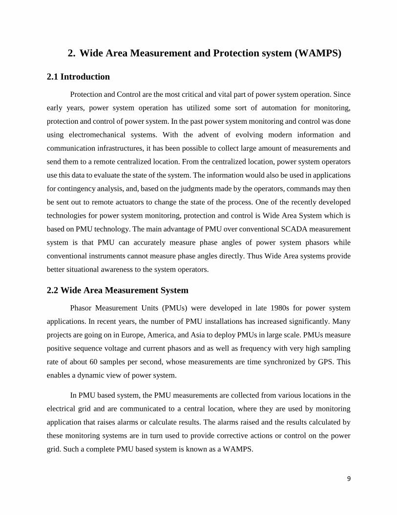
Phasors are representations of sinusoids in complex plane. In phasor domain, sinusoid of (2.1) is

given by:

𝑥 (𝑡) = 𝑅𝑒 {𝑋𝑚𝑒𝑗(𝑤𝑡+∅)} (2.2)

𝑋 = 𝑋𝑚

√2𝑒𝑗(∅)

= 𝑋𝑟 + 𝑖𝑋𝑖 (2.3)

Where, 𝑋𝑟 is the real and 𝑋𝑖 is the imaginary component of the phasor.

The magnitude of the phasor is the rms value of the sinusoid and its phase angle is the

phase angle of the signal in (2.1). It is to be noted that the mathematical expression of (2.3) does

not include frequency. Phasors are defined at a particular frequency. The sinusoidal signal and its

phasor representation are shown in figure 2.3.

Fig. 2.3: Phasor representation of a sinusoidal signal

Positive sequence voltages of a network constitute the state vector of a power system, and

it is of fundamental importance in all forms of power system analysis. The positive sequence

phasor can be computed according to its definition as:

𝑋1 =1

3(𝑋𝑎 + 𝛼𝑋𝑏 + 𝛼2𝑋𝑐) (2.4)

where, 𝛼 = 𝑒2𝜋𝑖

3

13

2.3.2 Architecture of Phasor Measurement Unit

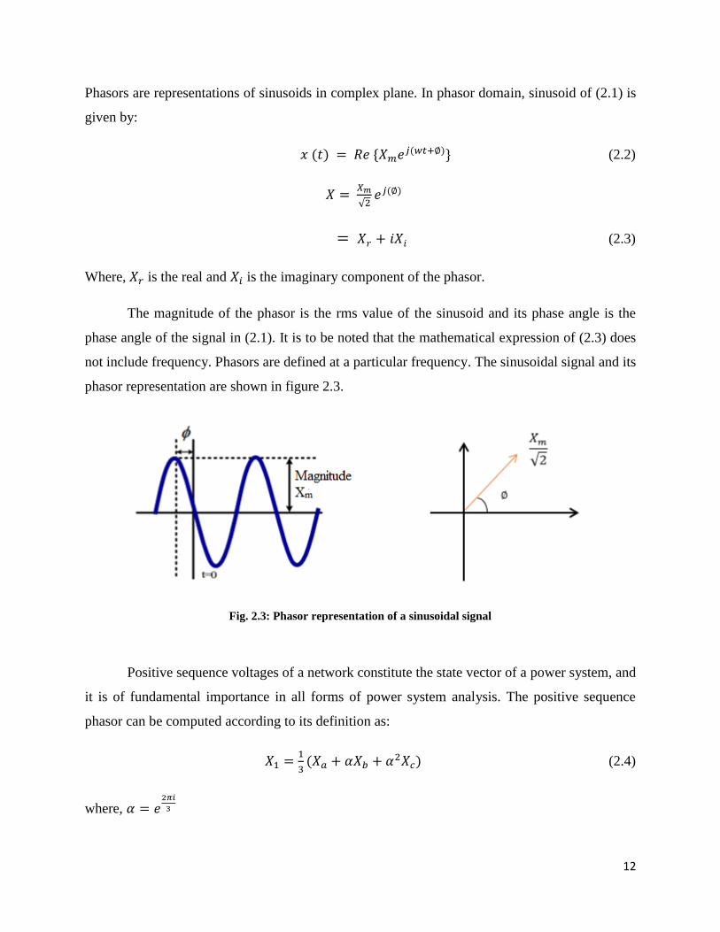
PMUs are designed to measure the positive sequence voltage and current phasors at very

high measurement rates, up to 60 measurements per second. The block diagram of PMU is shown

in figure 2.4. PMUs receive analog inputs such as 3-phase voltages, 3-phase and neutral currents

from the secondary of the voltage transformers and current transformers. The analog input signals

are then filtered by the anti-aliasing filter to avoid aliasing errors. Anti-aliasing filters limit the

bandwidth of voltage and current signals below the half of the sampling frequency to avoid

aliasing. Anti-aliasing filters introduce frequency dependent phase delays which are compensated

before synchrophasors are reported. The GPS signal is used to provide a time stamp for each

measurement using coordinated universal time as the reference. The GPS receiver provides the 1

pulse-per-second (pps) signal, and a time tag consisting of the year, day, hour, minute, and second.

The l-pps signal is usually divided by a phase-locked oscillator into the number of pulses per

second required for the sampling of the analogue signals. For analog to digital conversion a

mathematical method, Discrete Fourier Transform (DFT) is applied to estimate the fundamental

frequency components of the measured analog signal whose samples are taken at appropriate

intervals. Consider a periodic discrete-time finite signal with sampling time interval as2𝜋

𝑁. The

Fourier transform can be expressed as [15]

𝑋 =√2

𝑁∑ 𝑥𝑘𝑒

−𝑗2𝜋𝑘

𝑁𝑁𝑘=1 (2.5)

where,

X is the phasor representing the sinusoidal signal

𝑥𝑘 is the kth sample

N is the number of samples

A factor 2 usually appears in front of the sum as the signal with frequency 𝜔 as DFT has

components at + 𝜔 and - 𝜔.These components can be combined and divided by square root

of 2 to get the RMS value.

The microprocessor calculates the positive sequence voltage and current phasors, and

determines the timing message from the GPS, along with the sample number at the beginning of a

window [16].

14

Fig. 2.4: Block Diagram of PMU

2.4 Communication Network

Communication system plays a vital role for real time monitoring of power system. PMUs

are scattered over a wide geographical area far away from the control center. Effective

communication networks are needed to communicate PMU data to the control center. Reliability,

security and speed are the utmost important parameters for WAMS communication networks [17].

Power utilities generally use dedicated networks for WAMS communications.

Communication delay impacts dynamic grid monitoring and control. Many synchrophasor

applications are affected by the communication delays. Communication delay of a WAMS

network depends on the network bandwidth, propagation delay, communications buffering,

multiplexing, etc. The maximum data transmission rate of a communication network depends on

the available bandwidth of the network. If the data sending rate is more than the usable network

bandwidth there will be increase of communication delay. The propagation delay of a

communication network mainly depends on the communication medium. Following

communication mediums [18] have been considered for WAMS communications:

GPS Receiver

Phase-locked oscillator

A/D converter Microprocessor Anti-aliasing filters

Analog inputs

From C.T/V.T

Phasor

Communication

module

To PDC GPS

15

Telephone line: One of the basic communication mediums for the power utilities is

Telephone line. Telephone lines are economical and easy to set up. However, telephone

lines are slow and thus not suitable for synchrophasor communications.

Satellites: Low-earth orbiting (LEO) satellites can be used for synchrophasor

communications. These satellites have been used for SCADA communications. However,

these satellites are costly and have narrow bandwidths [18].

Power lines: Power line communication (PLC) is a technique in which power lines are

used as communication medium. Currently, PLC is being considered for WAMS

communications. The advantage of this technology is that the remote substations can be

easily reached via transmission lines [18]. High signal attenuations and distortions are the

main issues with this medium.

Microwave links: Microwave links have been used by utilities to connect remote PMUs

to a PDC when a wired connection is not economically possible. Signal fading and

multipath propagation are the main issues with this technology.

Fiber optic cables: Fiber optic based wired digital communication networks are

considered as most attractive for WAMS communications. Fiber optic cables can be used

for comparatively long distance transmissions without signal enhancements. Low latency,

large bandwidth and immunity to electromagnetic interference are the main advantages of

fiber optic communications [18]. The main disadvantage of this type of communication

medium is its high installation cost.

Communication systems in power system operation and control typically contain a mixture of

technologies and protocols. Apart from communication medium, PMUs need to use

communication protocol to send synchrophasor data to PDCs. Different communication protocols

have been used by different PMU manufacturers. DNP, Modbus, IEC 60870- 101 are some of the

early developed communication protocols. Internet protocols are increasingly being used for

WAMS communications. These internet protocols are mostly used over Ethernets. Commonly

used internet protocols for WAMS communications are TCP-only, UDP-only and TCP/UDP [6].

TCP is more reliable protocol than UDP. TCP works on hand-shaking principle. In the TCP

protocol, missed packets are sent again to the destination address [6]. So, missed packets actually

delay the communication of consecutive packets. The UDP protocol requires lesser bandwidth

16

than the TCP protocol [17]. In the UDP protocol, missed packets are not retransmitted [6]. So,

there is no additional delay in resending the missed packets.

2.4.1 Error-Dependent Communication Strategy

As communication system is an important component of control system, scalability of the

system is a concern; therefore, one of the first issues is how to communicate information about a

physical process. For example, one of the issues is timing for sampling and communication.

Traditional approach is to sample the physical process periodically or at predetermined

timestamps. An alternative is to sample it when specific events occur. Event-based sampling

requires continuous monitoring of the system to decide when to sample it. In this work, we study

the effect of event based message generation for detecting and locating faults on a transmission

system using PMU based technology. In [12] it is seen that the problem of tracking a dynamical

system over a network, if message generation and communication have correlation with estimation

error, has the same performance as the periodic sampling and communication method can be

reached using a significantly lower rate of data.

According to power system communication protocols, DNP3 or IEC 61850,

communication enabled devices can work in 2 possible modes:

Non-Event-driven mode (i.e., polling based)

Event-driven mode

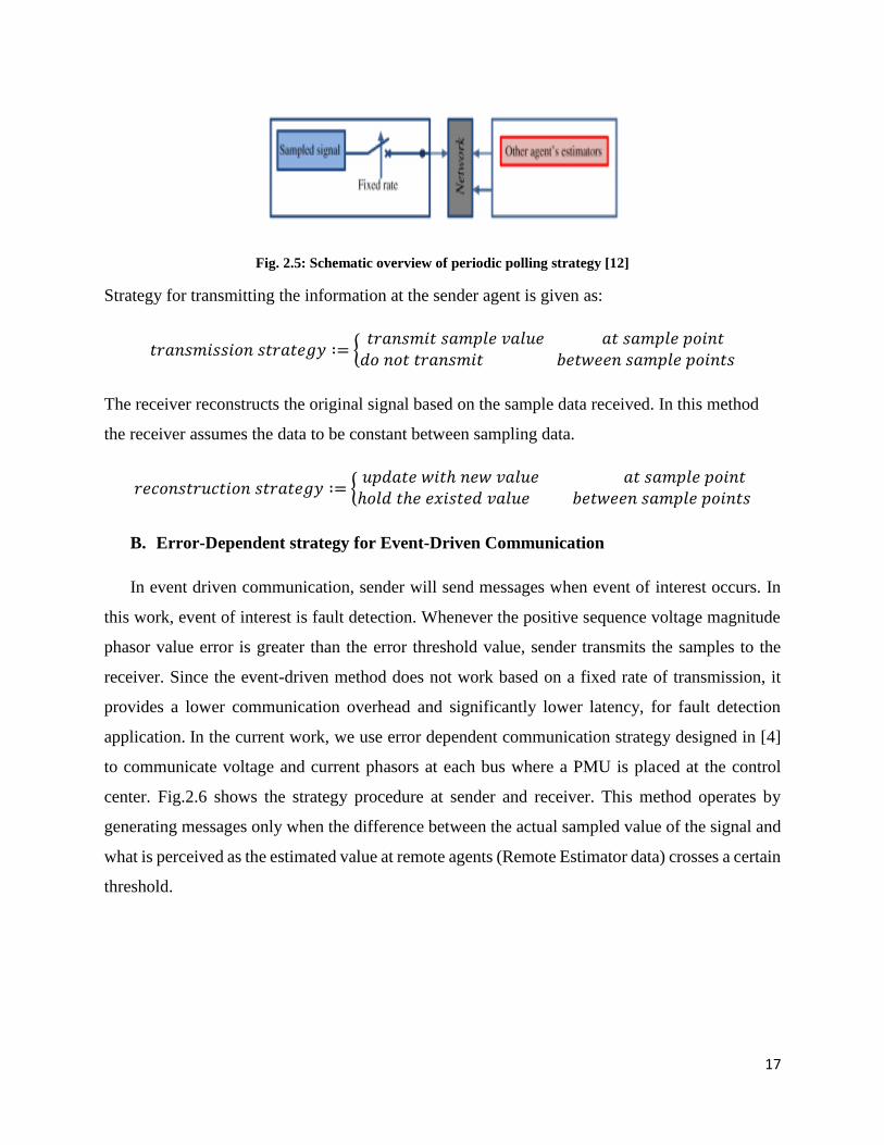
A. Non-Event-driven mode (Periodic Polling)

In this method, the transmitter samples continuous signal based on fixed rate of sampling; the

samples are then used to generate messages at each sample time.

Fig. 2.5 shows an overview of this system showing sender on left hand side and receiver on

the right hand side.

17

Fig. 2.5: Schematic overview of periodic polling strategy [12]

Strategy for transmitting the information at the sender agent is given as:

𝑡𝑟𝑎𝑛𝑠𝑚𝑖𝑠𝑠𝑖𝑜𝑛 𝑠𝑡𝑟𝑎𝑡𝑒𝑔𝑦 ∶= {𝑡𝑟𝑎𝑛𝑠𝑚𝑖𝑡 𝑠𝑎𝑚𝑝𝑙𝑒 𝑣𝑎𝑙𝑢𝑒 𝑎𝑡 𝑠𝑎𝑚𝑝𝑙𝑒 𝑝𝑜𝑖𝑛𝑡

𝑑𝑜 𝑛𝑜𝑡 𝑡𝑟𝑎𝑛𝑠𝑚𝑖𝑡 𝑏𝑒𝑡𝑤𝑒𝑒𝑛 𝑠𝑎𝑚𝑝𝑙𝑒 𝑝𝑜𝑖𝑛𝑡𝑠

The receiver reconstructs the original signal based on the sample data received. In this method

the receiver assumes the data to be constant between sampling data.

𝑟𝑒𝑐𝑜𝑛𝑠𝑡𝑟𝑢𝑐𝑡𝑖𝑜𝑛 𝑠𝑡𝑟𝑎𝑡𝑒𝑔𝑦 ∶= {𝑢𝑝𝑑𝑎𝑡𝑒 𝑤𝑖𝑡ℎ 𝑛𝑒𝑤 𝑣𝑎𝑙𝑢𝑒 𝑎𝑡 𝑠𝑎𝑚𝑝𝑙𝑒 𝑝𝑜𝑖𝑛𝑡ℎ𝑜𝑙𝑑 𝑡ℎ𝑒 𝑒𝑥𝑖𝑠𝑡𝑒𝑑 𝑣𝑎𝑙𝑢𝑒 𝑏𝑒𝑡𝑤𝑒𝑒𝑛 𝑠𝑎𝑚𝑝𝑙𝑒 𝑝𝑜𝑖𝑛𝑡𝑠

B. Error-Dependent strategy for Event-Driven Communication

In event driven communication, sender will send messages when event of interest occurs. In

this work, event of interest is fault detection. Whenever the positive sequence voltage magnitude

phasor value error is greater than the error threshold value, sender transmits the samples to the

receiver. Since the event-driven method does not work based on a fixed rate of transmission, it

provides a lower communication overhead and significantly lower latency, for fault detection

application. In the current work, we use error dependent communication strategy designed in [4]

to communicate voltage and current phasors at each bus where a PMU is placed at the control

center. Fig.2.6 shows the strategy procedure at sender and receiver. This method operates by

generating messages only when the difference between the actual sampled value of the signal and

what is perceived as the estimated value at remote agents (Remote Estimator data) crosses a certain

threshold.

18

Netw

ork

Other agent’s Estimators

Sampled signal

Scheduler

Remote Estimator

tx

x t

Fig. 2.6: Block diagram of procedure for Error-Dependent Communication Strategy [12]

In Fig.2.6 “remote estimator”, in the sender, saves a copy of its transmitted samples and

replicates the same process as the estimator that is running at the receivers. The sender would be

able to estimate and read the output of the remote estimator (�̃�(𝑡)) to calculate the estimation error

at the remote agents. According to this policy of transmission [12], the error,

𝑒(𝑡) = ‖𝑥(𝑡) − �̃�(𝑡)‖2 (2.5)

is considered in a message generation scheme to decide whether a new message should be

transmitted or not. The decision is simply based on a 𝑒(𝑡) crossing a predefined

threshold 𝑒𝑡ℎ.Therefore, the transmission strategy, executed in small timestamps (at the signal

sampling rate, 5 kHz), is as follows:

Transmission strategy ∶= {𝑡𝑟𝑎𝑛𝑠𝑚𝑖𝑡 𝑥(𝑡) 𝑖𝑓 𝑒(𝑡) > 𝑒𝑡ℎ

𝑑𝑜 𝑛𝑜𝑡 𝑡𝑟𝑎𝑛𝑠𝑚𝑖𝑡 𝑖𝑓 𝑒(𝑡) ≤ 𝑒𝑡ℎ

Remote estimator predicts the next value of state variable based on the recent information

transmitted through the network. Thus, it is essential to build models which are good representation

of sampled signal, for use in receiver’s estimator and sender’s remote estimator. Linear prediction

[57] [58] is used to model the sampled signal as it recursively represents sampled signal based on

past values of the signal. Auto regressive model (all poles) is applied to fit on the sample values

as follows [12]:

x(t) = 𝑎1𝑥(𝑡 − 𝑇) + 𝑎2𝑥(𝑡 − 2𝑇) + ⋯+ 𝑎𝑛𝑥(𝑡 − 𝑛𝑇) (2.6)

where, x (t) is sampled signal at time t,

T is sampling time,

19

𝑎1, 𝑎2, … , 𝑎𝑛 are coefficients of linear prediction and

n indicates the degree of model.

The best fit on the sample times can be found by considering two steps:

Selecting the model degree n and

Predicting the sample value for times ahead based on coefficients of linear predictor

Least square error method is one of the methods for finding the best coefficients for linear

prediction model. Considering that any estimation includes estimation error, for time t-1,

equation (2.6) can be rewritten as:

𝑥(t − T) = 𝑎1𝑥(𝑡 − 2𝑇) + 𝑎2𝑥(𝑡 − 3𝑇) + ⋯+ 𝑎𝑛𝑥(𝑡 − (𝑛 + 1)𝑇) + 𝑒(𝑡 − 𝑇) (2.7)

where, 𝑒(𝑡 − 𝑇) is the estimation error. Vector representation of equation (2.7) is given by:

𝑥(𝑡 − 𝑇) = 𝜑𝑇(𝑡 − 𝑇)𝜃 + 𝑒(𝑡 − 𝑇) (2.8)

where, 𝜑 is the data vector, and 𝜃 is the coefficients vector. The vector 𝜑 and 𝜃 are given by:

𝜑(𝑡 − 𝑇) = [𝑥(𝑡 − 2𝑇) 𝑥(𝑡 − 3𝑇)…𝑥(𝑡 − (𝑛 + 1)𝑇)]𝑇 (2.9)

𝜃 = [𝑎1 𝑎2 … 𝑎𝑛]𝑇 (2.10)

If the sample values are available from 𝑡 − (𝑚 + 𝑛)𝑇 to 𝑡 − 𝑇 in the remote estimator, (2)

can be represented as follows:

𝑋 = 𝜑𝜃 + 𝑒 (2.11)

𝑋 = [

𝑥(𝑡 − 𝑇)𝑥(𝑡 − 2𝑇)

⋮𝑥(𝑡 − 𝑚𝑇)

] , 𝜑 =

[

𝜑𝑇(𝑡 − 𝑇)

𝜑𝑇(𝑡 − 2𝑇)⋮

𝜑𝑇(𝑡 − 𝑚𝑇)] , 𝑒 = [

𝑒(𝑡 − 𝑇)𝑒(𝑡 − 2𝑇)

⋮𝑒(𝑡 − 𝑚𝑇)

] (2.12)

where, m is the window length. As least square method delivers the best coefficients based on

minimizing the energy of the estimation error term, the following cost function is minimized in

this method as:

20

𝐽(𝜃) =1

2∑ (𝑥(𝑡 − 𝑖𝑇) − 𝜑𝑇(𝑡 − 𝑖𝑇)𝜃)2 𝑚

𝑖=1

=1

2[𝑋 − 𝜑𝜃]𝑇[𝑋 − 𝜑𝜃] (2.13)

The extremum of the cost function with respect has to satisfy the following condition:

𝜕𝐽(𝜃)

𝜕𝜃= [𝑋 − 𝜑𝜃]𝑇[−𝜑] = 0 (2.14)

As the second derivative of the cost function is positive, the extremum point of the cost

function is a minimum, and the coefficients vector, which satisfies the minimum point condition,

is given by:

𝜃 = (𝜑𝑇𝜑)−1𝜑𝑇𝑋 (2.15)

Based on availability of sample values, for predicting next sample value two models are

proposed. First model is based on selecting straight line to fit on existing data (the last two samples)

and to find the next sample value at each sample time instance. Coefficients are fixed in this

method. In second model, coefficients are not fixed and they are calculated at each sample time

instance based on the available transmitted samples. Model order and window length should be

determined before the communication process for calculating coefficients. Larger window length

needs more past sample values and thus can yield more precise estimation. But if model degree is

chosen too high, over parameterized estimation (matrix 𝜑𝑇𝜑 becomes singular) happens. Thus,

best way would be to choose n small enough to have a good estimation. Based on equation (2.15),

coefficients are calculated and the next value is predicted based on the coefficients and previous

sample values. The method of estimation in remote estimator is given as:

�̃�(𝑡) = 𝑎1𝑥(𝑡 − 𝑇) + 𝑎2𝑥(𝑡 − 2𝑇) + ⋯+ 𝑎𝑛𝑥(𝑡 − 𝑛𝑇) (2.16)

Hence, the strategy at receiver side is given by:

𝑟𝑒𝑐𝑜𝑛𝑠𝑡𝑟𝑢𝑐𝑡𝑖𝑜𝑛 𝑠𝑡𝑟𝑎𝑡𝑒𝑔𝑦 ∶= {𝑥(𝑡) 𝑖𝑓 𝑛𝑒𝑤 𝑣𝑎𝑙𝑢𝑒 𝑖𝑠 𝑟𝑒𝑐𝑒𝑖𝑣𝑖𝑒𝑑

𝑎1𝑥(𝑡 − 𝑇) + ⋯+ 𝑎𝑛𝑥(𝑡 − 𝑛𝑇) 𝑂𝑡ℎ𝑒𝑟𝑤𝑖𝑠𝑒

21

The window length considered for this work is 3 and error threshold 𝑒𝑡ℎ is 0.001V (p.u.). There

will be no communication when system is in normal state i.e. positive sequence voltage magnitude

is greater than 0.9. When fault occurs, as voltage magnitude drops, the sender transmits new

sample values based on predefined error threshold.

22

3. Linear State Estimation

Effective Control and operation of electric power systems is based on the ability to

determine the system's state in real time. Power system state estimation (SE) was introduced in the

late 60s in order to achieve this objective and has traditionally been treated as a static state

estimation problem. This involved collection of various measurements like voltage magnitudes,

current injections; real and reactive power flows etc., such that there are more measurements than

state variables, thus forming an over determined system. These measurements were assigned a

weight based on their accuracy and form nonlinear “load flow-like” equations which required

multiple iterations to arrive at a solution. The solution of this minimization was the system state.

Then operators could use this information to make decisions regarding the control and operation

of their power system. The measurements are available through SCADA system [19] [20] and are

communicated using Remote Terminal Unit (RTU).Measurements are available from SCADA

system every 4 to 10 seconds, thus providing a static state estimation. Also computational time of

nonlinear iterations adds to the delay in estimating the system state. With the advancement in

development of PMUs, accurate and dynamic state estimation has been made possible. PMUs

provide measurements at the rate of 60 samples per second which are synchronized using GPS

system, thus eliminating the delay time occurring in traditional state estimator. Also, traditional

nonlinear equations which require high computation time can be replaced by linear equations

formed using voltage and current phasor measurements given by PMU, thus simplifying the

estimation process. In this chapter, firstly mathematical basis for traditional state estimation is

discussed which is then followed by formulation of equations for linear state estimation process to

improve the quality of state estimation.

3.1 Traditional State Estimation

Power system state estimation requires various measurements to estimate the state of the

system. The measurement data which is used by state estimator is a subset of “real-time” data

obtained from SCADA system which includes voltage magnitudes, current magnitudes, power

flow values and power injections. State estimator also requires “static” database containing

information regarding connectivity of circuit breakers and bus section which is always stored in

the control center. With both the real-time database and static database, State Estimation process can

23

estimate the system state by executing the functions [31] described below in the order shown in Fig.

3.1.

Topology processing: uses the real-time circuit breaker status with the substation and

system level topology to determine the connectivity of the whole network.

Observability analysis: Given a set of measurements, determines if there exists a state

estimation solution for the entire system or part of the system, and identifies the

unobservable branches and the observable islands in the system if exist [32] [33].

State estimation: solves for the complex voltages at each bus from the real-time analog

measurements.

Bad data processing: tests the solution to find bad measurements (and if found, reruns the

SE solution without the bad data) [34].

Fig. 3.1: Flow chart of Traditional State Estimator

3.1.1 Component Modelling

For state estimation, various components of power system like transmission lines, shunt

capacitors or reactors, transformers have to be modelled. Also, topology information is required

which specifies how these components are connected to form electric power network.

Transmission lines in power system are three phase. Let us assume transmission lines are fully

transposed and all other shunt and series devices are symmetrical in all the three phases. Also

generation and load in each phase are assumed to be balanced. Thus, single phase analysis can be

used to simplify the model, which is represented by two-port 𝜋 equivalent model [35].All the

parameters are assumed to be in per unit.

Topology

Processor

State

Estimation

Bad Data

Processing

Observability

Analysis System

States

Yes

No

24

The transmission line model used in most state estimation techniques uses only four

parameters to describe the transmission line shown in Fig. 3.2. The resistance models the real

copper losses in the conductor and the inductor models the energy stored in the magnetic field

surrounding the conductor. The shunt impedance (usually just the susceptance) models the line

charging. However, the shunt impedance is often entirely neglected especially on lower voltage

systems [36].

Fig. 3.2: Two-port model of a transmission line

Similarly transformer can be modelled as shown in Fig. 3.3. It has series impedance and

shunt impedance. The resistance of the series impedance models the real losses in the copper coils

and the inductance results from the fact that the conductors are arranged in a coil. The shunt

impedance includes a real part which results from eddy current losses and an imaginary part (or

magnetizing impedance) that results from the hysteresis losses. Both transmission lines and

transformers have a sending and receiving end that serve as its connections to two different nodes

in the network. Other types of transformers are modeled differently. For example, phase shifting

transformers include a phase offset multiplier in the total impedance of the transformer branch

Fig. 3.3: Transformer branch model

25

Tap changing transformers work similarly though the tap setting, a, may be included as a

state variable. They are modeled using series impedance in series with the transformer model.

Fig. 3.4: Tap-changing transformer

Shunt capacitors and reactors are devices which are installed in the network to serve as reactive

power support and voltage control. These are represented by their per phase susceptance at

corresponding bus.

3.1.2 The Bus-Admittance Matrix

Various network parameters such as transmission line series and shunt impedances,

transformer impedances, and shunt capacitors and reactors which have been defined already can

be assembled together to construct the network model of the system. This is called the admittance

matrix or the Y-Bus of the power system. The admittance matrix of a power system is given as:

𝐼 = [

𝑖1𝑖2⋮𝑖𝑛

] = [

𝑌11 𝑌12 … 𝑌1𝑁

𝑌21 𝑌22 … 𝑌2𝑁

⋮𝑌𝑁1

⋮𝑌𝑁2

⋱…

⋮𝑌𝑁𝑁

] [

𝑉1

𝑉2

⋮𝑉𝑁

] = 𝑌 ∗ 𝑉 (3.1)

Admittances are used instead of impedances because the admittance matrix can be populated

by inspection while the corresponding impedance matrix is extremely difficult to populate by hand.

The rules for populating the admittance matrix of a network are derived from Kirchhoff’s laws of

current injections into a node. Sparing the derivation of the equations, there are two simple rules

that can be used to construct the network admittance matrix by inspection.

26

1. The 𝑚𝑚𝑡ℎ element of the admittance matrix is the sum of the admittances of all of the lines

connected to bus m.

2. The 𝑚𝑛𝑡ℎ element of the admittance matrix is the negative of the admittance connecting

bus m to bus n.

The admittance matrix is generally complex in nature, structurally symmetric, very sparse for large

networks, and nonsingular provided that each island contains a connection to ground [36].

3.1.3 Maximum Likelihood Estimation

Maximum likelihood estimation is a statistical method employed to estimate the states of

the system. Firstly likelihood function of measurement vector is created. The likelihood function

is simply the product of each of the probability density functions of each measurement. Maximum

likelihood estimation aims to estimate the unknown parameters of each of the measurements’

probability density functions through an optimization [36]. The probability density function for

power system measurement errors is the normal (or Gaussian) probability density function.

𝑓(𝑧) =1

√2𝜋𝜎𝑒

−1

2{𝑧−𝜇

𝜎}2

(3.2)

where, z is random variable of the probability density function,

𝜇 is the expected value

𝜎 is the standard deviation

This function would yield the probability of a measurement being a particular value, z. Therefore,

the probability of measuring a particular set of m measurements each with the same probability

density function is the product of each of the measurements probability density functions, or the

likelihood function for that particular measurement vector [36].

𝑓𝑚(𝑧) = ∏ 𝑓(𝑧𝑖)𝑚𝑖=1 (3.3)

where 𝑧𝑖 is the 𝑖𝑡ℎ measurement and

[𝑧] =

[ 𝑧1

𝑧2𝑧𝑐

⋮𝑧𝑚]

(3.4)

27

Maximum likelihood estimation aims to maximize this function to determine the unknown

parameters of the probability density function of each of the measurements. This can be done by

maximizing the logarithm of the likelihood function, 𝑓𝑚(𝑧) or minimizing the weighted sum of

squares of the residuals [36]. This can be written as

𝑚𝑖𝑛𝑖𝑚𝑖𝑧𝑒 ∑ 𝑊𝑖𝑖𝑟𝑖2𝑚

𝑖=1 (3.5)

𝑠𝑢𝑏𝑗𝑒𝑐𝑡 𝑡𝑜 𝑧𝑖 = ℎ𝑖(𝑥) + 𝑟𝑖

The solution to this problem is referred to as the weighted least squares (WLS) estimator for x.

3.1.4 Weighted Least Squares State Estimation

The state estimator becomes a weighted least squares estimator with the inclusion of the

measurement error covariance matrix which serves to weigh the accuracy of each of the

measurements. The physical system model information and measurements are part of the equality

constraints of the basic weighted least squares optimization and are what make this algorithm

specific to power systems.

A. WLS Algorithm:

Mathematical algorithms for weighted least square estimator are presented in various papers in the

past [22] [36]. Consider a measurement vector denoted by z containing m number of measurements

and a state vector denoted by x containing n number of state variables.

[𝑧] = [

𝑧1

𝑧2

⋮𝑧𝑚

] [𝑥] = [

𝑥1

𝑥2

⋮𝑥𝑛

] (3.6)

Traditional state estimation techniques employ measurement sets which are nonlinear functions

of the system state vector. These functions are denoted by ℎ𝑖(𝑥) and can be assembled in vector

form as well.

[ℎ𝑖(𝑥)] =

[ ℎ1(𝑥1 𝑥2 … 𝑥𝑛)

ℎ2(𝑥1 𝑥2 … 𝑥𝑛)

⋮ℎ𝑚(𝑥1 𝑥2 … 𝑥𝑛)]

(3.7)

28

All of these measurements have their own unknown error associated with them denoted by e and

is given as

[𝑒] = [

𝑒1

𝑒2

⋮𝑒𝑚

] (3.8)

The measurement errors are assumed to be independent of one another and have an

expected value of zero. The state equation using non-linear functions to relate the system state

vector to the set of measurements can now be written in its complete form.

[𝑧] = [ℎ(𝑥)] + [𝑒] (3.9)

The solution to the state estimation problem can be formulated as a minimization of

following objective function.

𝐽(𝑥) = ∑(𝑧𝑖−ℎ𝑖(𝑥))2

𝑅𝑖𝑖

𝑚𝑖=1 (3.10)

This represents the summation of the squares of the measurement residuals weighted by

their respective measurement error covariance. This can be rewritten as the following

𝐽(𝑥) = [𝑧 − ℎ(𝑥)]𝑇𝑅−1[𝑧 − ℎ(𝑥)] (3.11)

Where R is the covariance matrix of the measurement errors and is diagonal in structure.

Each of the diagonal elements is the covariance of its respective measurement and all of the off-

diagonal elements are zero because the measurements are assumed to be independent. To find the

minimum of this objective function the derivative should be zero. The derivative of the objective

function is denoted by g(x).

𝑔(𝑥) =𝜕𝐽(𝑥)

𝜕𝑥= −[𝐻]𝑇𝑅−1[𝑧 − ℎ(𝑥)] (3.12)

𝑤ℎ𝑒𝑟𝑒 [𝐻] =𝜕ℎ(𝑥)

𝜕𝑥 (3.13)

29

The matrix H(x) is called the measurement Jacobian matrix. Ignoring the higher order terms

of the Taylor series expansion of the derivative of the objective functions yields an iterative

solution known as the Gauss-Newton method.

𝑥𝑘+1 = 𝑥𝑘 + [[𝐻(𝑥𝑘)]𝑇[𝑅]−1[𝐻(𝑥𝑘)]]−1[[𝐻(𝑥𝑘)]𝑇[𝑅]−1[𝑧 − ℎ(𝑥𝑘)]] (3.14)

It can be seen that only information required to iteratively solve this optimization is the

covariance matrix of measurement errors, R, and the measurement function, h(x). The

measurement Jacobian, H(x) is simply the derivative of the measurement function with respect to

the state vector. The measurement function and measurement Jacobian can be constructed using

the known system model including branch parameters, network topology, and measurement

locations and type. The error covariance matrix should also be constructed prior to the iterations

with the accuracy information of the meters installed in the system.

For the first iteration of the optimization the measurement function and measurement

Jacobian should be evaluated at flat voltage profile, or flat start. A flat start refers to a state vector

where all of the voltage magnitudes are 1.0 per unit and all of the voltage angles are 0 degrees. In

conjunction with the measurements, the next iteration of the state vector can be calculated again

and again until a desired tolerance is reached.

B. The Measurement Function

Various types of measurements such as real and reactive bus injections and flows, voltage

magnitudes, current magnitudes etc., are involved in the state estimation calculation. In this thesis

two-port 𝜋 equivalent model of transmission line is assumed and the measurement parameters are

derived based on this model.

Fig. 3.5: Two-port 𝝅 equivalent model of transmission line

30

Firstly, let us formulate real and reactive bus injections. For an injection at bus, the

measurements can be expressed as functions of the state vector (if the state vector is expressed in

polar coordinates) and elements of the bus-admittance matrix. N is the total number of busses

connected to bus m.

𝑃𝑚 = 𝑉𝑚 ∑ 𝑉𝑛(𝐺𝑚𝑛𝑐𝑜𝑠𝜃𝑚𝑛 + 𝐵𝑚𝑛𝑠𝑖𝑛𝜃𝑚𝑛)𝑁𝑛=1 (3.15)

𝑄𝑚 = 𝑉𝑚 ∑ 𝑉𝑛(𝐺𝑚𝑛𝑠𝑖𝑛𝜃𝑚𝑛 − 𝐵𝑚𝑛𝑐𝑜𝑠𝜃𝑚𝑛)𝑁𝑛=1 (3.16)

The conductance and susceptance follow the notation of the two port model given in

Fig.3.4.Similarly real and reactive power flows are given as

𝑃𝑚𝑛 = 𝑉𝑚2(𝑔𝑚 + 𝑔𝑚𝑛) − 𝑉𝑚𝑉𝑛(𝑔𝑚𝑛𝑐𝑜𝑠𝜃𝑚𝑛 + 𝑏𝑚𝑛𝑠𝑖𝑛𝜃𝑚𝑛) (3.17)

𝑄𝑚𝑛 = −𝑉𝑚2(𝑏𝑚 + 𝑏𝑚𝑛) − 𝑉𝑚𝑉𝑛(𝑔𝑚𝑛𝑠𝑖𝑛𝜃𝑚𝑛 − 𝑏𝑚𝑛𝑐𝑜𝑠𝜃𝑚𝑛) (3.18)

The line current magnitude from bus m to bus n can be expressed as

𝐼𝑚𝑛 =√𝑃𝑚𝑛

2 +𝑄𝑚𝑛2

𝑉𝑚=

𝑆𝑚𝑛

𝑉𝑚 (3.19)

C. Measurement Jacobian

Measurement Jacobian is the derivative of the measurement function with respect to the state

vector. The measurement jacobian can be represented in matrix form and given as

[𝐻] =

[

𝜕𝑃𝑖𝑛𝑗

𝜕𝜃

𝜕𝑃𝑖𝑛𝑗

𝜕𝑉𝜕𝑃𝑓𝑙𝑜𝑤

𝜕𝜃

𝜕𝑃𝑓𝑙𝑜𝑤

𝜕𝑉

𝜕𝑄𝑖𝑛𝑗

𝜕𝜃𝜕𝑄𝑓𝑙𝑜𝑤

𝜕𝜃𝜕𝐼𝑚𝑎𝑔

𝜕𝜃

0

𝜕𝑄𝑖𝑛𝑗

𝜕𝑉𝜕𝑄𝑓𝑙𝑜𝑤

𝜕𝑉𝜕𝐼𝑚𝑎𝑔

𝜕𝑉𝜕𝑉𝑚𝑎𝑔

𝜕𝑉 ]

(3.20)

31

The order of the measurement vector will correspond to the order of the rows in the

measurement function, and therefore, the measurement Jacobian. Similarly, the columns will

correspond to the order of the state vector. Once constructed, the Jacobian matrix elements are

each non-linear functions of the state variable and are re-evaluated for each iteration of the

estimation solution. There are generalized equations for each type of element that may appear

inside of this matrix. These can be classified first by measurement type and second by variable

with which the derivative has been taken with respect to. First are the partial derivatives of the

Jacobian matrix elements corresponding to the real power injection measurements.

𝜕𝑃𝑚

𝜕𝜃𝑚= ∑ 𝑉𝑚𝑉𝑛(𝑁

𝑛=1 −𝐺𝑚𝑛𝑠𝑖𝑛𝜃𝑚𝑛 + 𝐵𝑚𝑛𝑐𝑜𝑠𝜃𝑚𝑛) − 𝑉𝑚2𝐵𝑚𝑚 (3.21)

𝜕𝑃𝑚

𝜕𝜃𝑛= 𝑉𝑚𝑉𝑛(𝐺𝑚𝑛𝑠𝑖𝑛𝜃𝑚𝑛 − 𝐵𝑚𝑛𝑐𝑜𝑠𝜃𝑚𝑛) (3.22)

𝜕𝑃𝑚

𝜕𝑉𝑚= ∑ 𝑉𝑛(𝑁

𝑛=1 𝐺𝑚𝑛𝑐𝑜𝑠𝜃𝑚𝑛 + 𝐵𝑚𝑛𝑠𝑖𝑛𝜃𝑚𝑛) − 𝑉𝑚𝐺𝑚𝑚 (3.23)

𝜕𝑃𝑚

𝜕𝑉𝑛= 𝑉𝑚(𝐺𝑚𝑛𝑐𝑜𝑠𝜃𝑚𝑛 + 𝐵𝑚𝑛𝑠𝑖𝑛𝜃𝑚𝑛) (3.24)

The partial derivatives of the Jacobian matrix elements corresponding to reactive power

injection measurements

𝜕𝑄𝑚

𝜕𝜃𝑚= ∑ 𝑉𝑚𝑉𝑛(𝑁

𝑛=1 𝐺𝑚𝑛𝑐𝑜𝑠𝜃𝑚𝑛 + 𝐵𝑚𝑛𝑠𝑖𝑛𝜃𝑚𝑛) − 𝑉𝑚2𝐺𝑚𝑚 (3.25)

𝜕𝑄𝑚

𝜕𝜃𝑛= −𝑉𝑚𝑉𝑛(𝐺𝑚𝑛𝑐𝑜𝑠𝜃𝑚𝑛 + 𝐵𝑚𝑛𝑠𝑖𝑛𝜃𝑚𝑛) (3.26)

𝜕𝑄𝑚

𝜕𝑉𝑚= ∑ 𝑉𝑛(𝑁

𝑛=1 𝐺𝑚𝑛𝑠𝑖𝑛𝜃𝑚𝑛 − 𝐵𝑚𝑛𝑐𝑜𝑠𝜃𝑚𝑛) − 𝑉𝑚𝐵𝑚𝑚 (3.27)

𝜕𝑄𝑚

𝜕𝑉𝑛= 𝑉𝑛(𝐺𝑚𝑛𝑠𝑖𝑛𝜃𝑚𝑛 − 𝐵𝑚𝑛𝑐𝑜𝑠𝜃𝑚𝑛) (3.28)

32

Next, the partial derivatives of the Jacobian matrix elements corresponding to real power

flow measurements are

𝜕𝑃𝑚𝑛

𝜕𝜃𝑚= 𝑉𝑚𝑉𝑛(𝑔𝑚𝑛𝑠𝑖𝑛𝜃𝑚𝑛 − 𝑏𝑚𝑛𝑐𝑜𝑠𝜃𝑚𝑛) (3.29)

𝜕𝑃𝑚𝑛

𝜕𝜃𝑛= −𝑉𝑚𝑉𝑛(𝑔𝑚𝑛𝑠𝑖𝑛𝜃𝑚𝑛 − 𝑏𝑚𝑛𝑐𝑜𝑠𝜃𝑚𝑛) (3.30)

𝜕𝑃𝑚𝑛

𝜕𝑉𝑚= −𝑉𝑛(𝑔𝑚𝑛𝑐𝑜𝑠𝜃𝑚𝑛 + 𝑏𝑚𝑛𝑠𝑖𝑛𝜃𝑚𝑛) + 2(𝑔𝑚 + 𝑔𝑚𝑛)𝑉𝑚 (3.31)

𝜕𝑃𝑚𝑛

𝜕𝑉𝑛= −𝑉𝑚(𝑔𝑚𝑛𝑐𝑜𝑠𝜃𝑚𝑛 + 𝑏𝑚𝑛𝑠𝑖𝑛𝜃𝑚𝑛) (3.32)

Partial derivatives of the Jacobian matrix elements corresponding to reactive power flow

measurements are given as

𝜕𝑄𝑚𝑛

𝜕𝜃𝑚= −𝑉𝑚𝑉𝑛(𝑔𝑚𝑛𝑐𝑜𝑠𝜃𝑚𝑛 + 𝑏𝑚𝑛𝑠𝑖𝑛𝜃𝑚𝑛) (3.33)

𝜕𝑄𝑚𝑛

𝜕𝜃𝑛= 𝑉𝑚𝑉𝑛(𝑔𝑚𝑛𝑐𝑜𝑠𝜃𝑚𝑛 + 𝑏𝑚𝑛𝑠𝑖𝑛𝜃𝑚𝑛) (3.34)

𝜕𝑄𝑚𝑛

𝜕𝑉𝑚= −𝑉𝑛(𝑔𝑚𝑛𝑠𝑖𝑛𝜃𝑚𝑛 − 𝑏𝑚𝑛𝑐𝑜𝑠𝜃𝑚𝑛) − 2(𝑏𝑚 + 𝑏𝑚𝑛)𝑉𝑚 (3.35)

𝜕𝑄𝑚𝑛

𝜕𝑉𝑛= −𝑉𝑚(𝑔𝑚𝑛𝑠𝑖𝑛𝜃𝑚𝑛 − 𝑏𝑚𝑛𝑐𝑜𝑠𝜃𝑚𝑛) (3.36)

Next we need to find partial derivate of voltage measurements. Note that the voltage

magnitude is not a function of voltage magnitudes or angles at any bus besides its own.

𝜕𝑉𝑖

𝜕𝑉𝑖= 1;

𝜕𝑉𝑖

𝜕𝑉𝑗= 0;

𝜕𝑉𝑖

𝜕𝜃𝑖= 0;

𝜕𝑉𝑖

𝜕𝜃𝑗= 0 (3.37)

33

Next are the partial derivatives of the Jacobian matrix elements corresponding to the

current magnitude measurements. For these equations the shunt branch has been ignored.

𝜕𝐼𝑚𝑛

𝜕𝜃𝑚=

𝑔𝑚𝑛2 +𝑏𝑚𝑛

2

𝐼𝑚𝑛𝑉𝑚𝑉𝑛𝑠𝑖𝑛𝜃𝑚𝑛 (3.38)

𝜕𝐼𝑚𝑛

𝜕𝜃𝑛= −


2

𝐼𝑚𝑛𝑉𝑚𝑉𝑛𝑠𝑖𝑛𝜃𝑚𝑛 (3.39)

𝜕𝐼𝑚𝑛

𝜕𝑉𝑚=


2

𝐼𝑚𝑛(𝑉𝑚 − 𝑉𝑛𝑐𝑜𝑠𝜃𝑚𝑛) (3.40)

𝜕𝐼𝑚𝑛

𝜕𝑉𝑛= −


2

𝐼𝑚𝑛(𝑉𝑚𝑐𝑜𝑠𝜃𝑚𝑛 − 𝑉𝑛) (3.41)

3.2 Linear State Estimation

Traditional state estimators are basically static state estimators due to their large scan times. With

the advent of PMU technology, the scan times have reduced greatly, thus proving a dynamic view

of the power system. PMU technology can be included in various forms in traditional state

estimator. Several methods to include phasor measurements in state estimation have been

mentioned in the past [23-27].Some of them mix the phasor measurements with the conventional

measurements and solve in the same manner as before, while few methods include the phasor

measurements in a linear post-processing step with the output of the conventional state estimator.

However, a true application of PMU technology to state estimation would have all of the traditional

measurements of real and reactive power injections and current and voltage magnitudes replaced

by bus voltage phasors and line current phasors. If only PMU measurements are used, there are

also no complications from the use of both polar and rectangular values in the state estimation

process, as would be done when including PMU measurements in traditional state estimators. Once

the problem of scan time has been erased, the only issue of time is the communication and

computational delay between the collection of the measurements and the employment of useful

information for decision making by the operation and control applications. To solve this problem

Error-dependent communication strategy [12] is employed in this work, thus ensuring efficient

34

communication between the PMU and control center. Additionally, the state of the system is

actually being directly measured when using PMUs as metering devices. However, estimation is

still necessary for including redundancy and bad data filtering. Due to high installation cost of

PMU, they cannot be placed at every bus. Because of this, the placement of the PMUs is critical

for achieving a fully observable system with a sufficient amount of measurement redundancy [37]

[38].

To understand the fundamental difference between the measurements used in a traditional

state estimator and the measurements used in a linear state estimator it is best to begin with a

simple two-port π-model equivalent of a transmission line.

Fig. 3.6 𝝅 section model of a transmission line

From Fig.3.5, let us assume PMU is installed at bus m, voltage phasors can be expressed in

rectangular form as [39]:

�̅�𝑚 = 𝑉𝑚𝑐𝑜𝑠𝜃𝑚 + 𝑗𝑉𝑚𝑠𝑖𝑛𝜃𝑚 (3.42)

�̅�𝑛 = 𝑉𝑛𝑐𝑜𝑠𝜃𝑛 + 𝑗𝑉𝑛𝑠𝑖𝑛𝜃𝑛 (3.43)

Where �̅�𝑚, �̅�𝑛are the voltage phasors at bus m and n respectively. The current phasor

measurements should be expressed in linear relationship with the states of the power system. The

current 𝐼�̅�𝑛 can be expressed as:

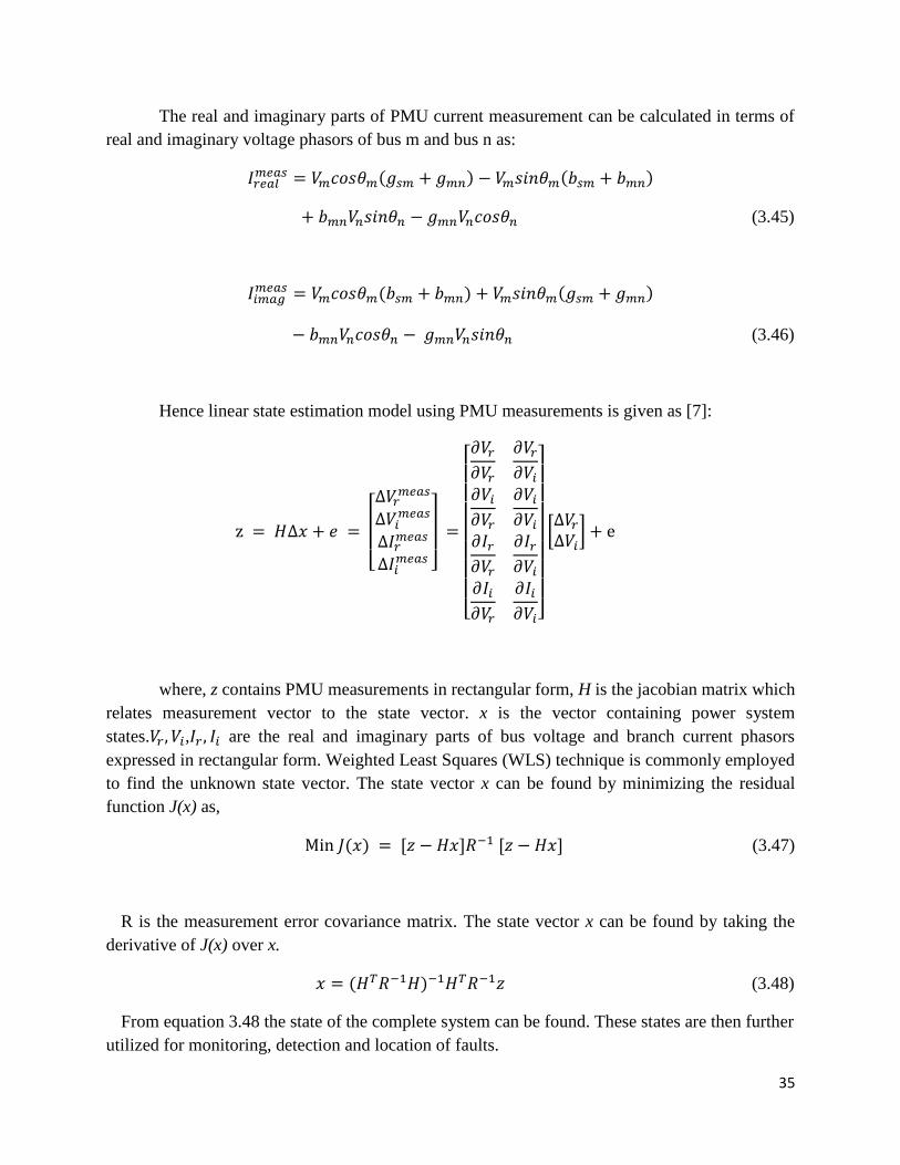
𝐼�̅�𝑛 = �̅�𝑚(𝑔𝑠𝑚 + 𝑗𝑏𝑠𝑚) + (�̅�𝑚 − �̅�𝑛)(𝑔𝑚𝑛 + 𝑗𝑏𝑚𝑛) (3.44)

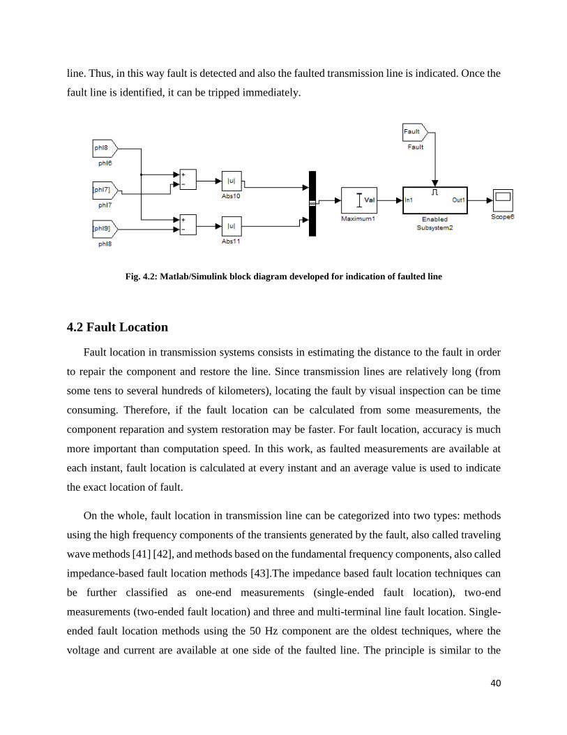
35

The real and imaginary parts of PMU current measurement can be calculated in terms of

real and imaginary voltage phasors of bus m and bus n as:

𝐼𝑟𝑒𝑎𝑙𝑚𝑒𝑎𝑠 = 𝑉𝑚𝑐𝑜𝑠𝜃𝑚(𝑔𝑠𝑚 + 𝑔𝑚𝑛) − 𝑉𝑚𝑠𝑖𝑛𝜃𝑚(𝑏𝑠𝑚 + 𝑏𝑚𝑛)

+ 𝑏𝑚𝑛𝑉𝑛𝑠𝑖𝑛𝜃𝑛 − 𝑔𝑚𝑛𝑉𝑛𝑐𝑜𝑠𝜃𝑛 (3.45)

𝐼𝑖𝑚𝑎𝑔𝑚𝑒𝑎𝑠 = 𝑉𝑚𝑐𝑜𝑠𝜃𝑚(𝑏𝑠𝑚 + 𝑏𝑚𝑛) + 𝑉𝑚𝑠𝑖𝑛𝜃𝑚(𝑔𝑠𝑚 + 𝑔𝑚𝑛)

− 𝑏𝑚𝑛𝑉𝑛𝑐𝑜𝑠𝜃𝑛 − 𝑔𝑚𝑛𝑉𝑛𝑠𝑖𝑛𝜃𝑛 (3.46)

Hence linear state estimation model using PMU measurements is given as [7]:

z = 𝐻∆𝑥 + 𝑒 =

[ ∆𝑉𝑟

𝑚𝑒𝑎𝑠

∆𝑉𝑖𝑚𝑒𝑎𝑠

∆𝐼𝑟𝑚𝑒𝑎𝑠

∆𝐼𝑖𝑚𝑒𝑎𝑠 ]

=

[ 𝜕𝑉𝑟

𝜕𝑉𝑟

𝜕𝑉𝑟

𝜕𝑉𝑖

𝜕𝑉𝑖

𝜕𝑉𝑟

𝜕𝑉𝑖

𝜕𝑉𝑖

𝜕𝐼𝑟𝜕𝑉𝑟

𝜕𝐼𝑟𝜕𝑉𝑖

𝜕𝐼𝑖𝜕𝑉𝑟

𝜕𝐼𝑖𝜕𝑉𝑖]

[∆𝑉𝑟∆𝑉𝑖

] + e

where, z contains PMU measurements in rectangular form, H is the jacobian matrix which

relates measurement vector to the state vector. x is the vector containing power system

states.𝑉𝑟 , 𝑉𝑖,𝐼𝑟 , 𝐼𝑖 are the real and imaginary parts of bus voltage and branch current phasors

expressed in rectangular form. Weighted Least Squares (WLS) technique is commonly employed

to find the unknown state vector. The state vector x can be found by minimizing the residual

function J(x) as,

Min 𝐽(𝑥) = [𝑧 − 𝐻𝑥]𝑅−1 [𝑧 − 𝐻𝑥] (3.47)

R is the measurement error covariance matrix. The state vector x can be found by taking the

derivative of J(x) over x.

𝑥 = (𝐻𝑇𝑅−1𝐻)−1𝐻𝑇𝑅−1𝑧 (3.48)

From equation 3.48 the state of the complete system can be found. These states are then further

utilized for monitoring, detection and location of faults.

36

4. Detection and Location of Faults on Wide Area System

Transmission lines are the backbone of the power system. Transmission lines are exposed

to faults that are caused by different reasons such as short circuits, birds, and storms. Most of these

faults result in mechanical damage of power lines which must be repaired before returning the line

to service. Also rugged terrain and geographical layout cause some sections of power transmission

lines to be difficult to reach. In such situations, if a transient fault is persistent for a longer period

of time, it may lead to system blackout. Therefore, accurate fault detection and location under a

variety of power system operating constraints and fault conditions is an important requirement.

With the development of synchrophasor technology, monitoring and protection of power system

against faults has become possible. The real time data obtained from PMU can be used to monitor

and detect any abnormalities that occur in the system. PMUs provide samples at the rate of 60

messages per cycle, thus providing dynamic view of power system. The main objective of this

work is to monitor, detect and locate faults accurately using Wide Area Measurement and

Protection System (WAMP), which is explained in detail in this chapter.

4.1 Fault Detection

The disturbance in the power system usually develops gradually; however some phenomena,

such as transient instability, can develop in a fraction of second. Regardless of the phenomena and

available measures, any protection/control procedure during an emergency should consist of the

following elements:

Identification and prediction: A fast identification of the specific phenomena, from the

power system parameters, is required to implement measures so as to return the power

system to a healthy state. An emergency may be identified from the primary consequences

which are either directly or not-directly observable from local measurements. Further,

secondary consequences need to be predicted to avoid adverse impact of protection/control

measures.

Classification: Disturbance classification is based on the constraints that are violated,

severity and combination of violations, time scale of the phenomena, and utility control

policy. Classification should include identification of the place of a disturbance.

Decisions and actions: The choice of the measures is strongly related to the level of priority

during emergency. These levels are to stop the degradation of the system, return the system

to a secure state, and consider the economic and social impacts.

37

Coordination: Different measures may be used to solve different problems. An

uncoordinated action may not be economical or secure (e.g. trip of the plant on under

frequency protection before operation of the last step of the system under-frequency

control). An intelligent coordination of the protection and control actions is a major

challenge and a major requirement for any successful emergency procedure.

Corrections: After control measures have been applied, the system can be in an improved

but unsatisfactory state. This is acceptable, since it may be advantageous to implement

initial measures to stop further degradation of the system and then to continue with more

optimal actions when time allows. For example, initial load can be shed merely to stop

rapid frequency decline; and additional load, required to return frequency to normal, can

be calculated more accurately.

Time scale: For any of the previous elements, available time is a vital factor in selecting

appropriate actions. A trade-off between optimal methods and time is very often required.

The decision time includes selection of the remedial measure and implementation of

remedial measure.

4.1.1 Procedure for Fault Detection

Fault detection or identification is the primary step in protection of power system. The PMU

measurements are communicated to the control center based on Error-dependent communication

strategy. These measurements are then utilized by the linear state estimator to estimate the state of

the complete system. The states obtained are employed for detection of faults in the system. In this

work, the fault identification technique comprises of two components [52] [61]. The first

component is the voltage reduction due to fault occurrence. The second component is the power

flow direction after fault occurrence. The phase angle is used to determine the direction of fault

current with respect to a reference quantity. The ability to differentiate between a fault in one

direction or other is obtained by comparing the phase angle of the operating voltage and current.

The voltage is usually used as the reference polarizing quantity. The normal power flow in a given

direction will result in the phase angle between the voltage and the current varying around its

power factor angle ±φ. When power flows in the opposite direction, this angle will become (180°±

φ). For a fault in the reverse direction, the phase angle of the current with respect to the voltage

will be (180°- φ) [53].

38

Procedure for fault detection scheme can be summarized in following steps:

1) Compare positive sequence voltage magnitude of all the buses at every instant and find

minimum voltage which is at ,say bus r

𝑉𝑟 = min {|𝑉1|, |𝑉2|, |𝑉3|, …… . , |𝑉𝑛|} (4.1)

Where r ∈ i, i=1, 2, 3…n (n is the number of buses). |𝑉𝑛| is the positive sequence voltage

magnitude state obtained from linear state estimator.

2) If the minimum value is less than the threshold value which is 0.7 in our case, fault is

detected and is located near bus r.

3) Compare the absolute differences of positive sequence current angles for all lines

connecting bus r and selecting the maximum one.

|∆𝐴𝑞| = max {|∆𝐴𝑟1|, |∆𝐴𝑟2|, |∆𝐴𝑟3|, … . , |∆𝐴𝑟𝑛|} (4.2)

where |∆𝐴𝑟𝑛| is the absolute difference of positive sequence current angle for a transmission

line connecting bus "r" with bus "n" This can be described as

|∆𝐴𝑟𝑛| = |𝐴𝑟𝑛 − 𝐴𝑛𝑟| (4.3)

Fig.4.1 shows the block diagram developed in Matlab/Simulink for location of nearest area to

the fault based on comparing positive sequence voltage magnitude states obtained from linear state

estimator. 𝑉1, 𝑉2. . 𝑉9 are the input signals of positive sequence voltage magnitudes states of 9 buses

in the network. The minimum voltage magnitude is indicated by the Minimum block which

identifies the value and/or position of the smallest element in each column of the input, or tracks

the minimum values in a sequence of inputs over a period of time. Any decrease in the signal

magnitude is indicated by the Detect Decrease block which determines if the input signal is strictly

less than its previous value or not, the status can be recognized as:

The output is "1", when the input signal is less than its previous value.

The output is "0", when the input signal is greater than or equal to its previous value.

39

The threshold value of the input signal is detected by the Interval Test block which outputs "1"

if the input is between the values specified by the Lower limit and Upper limit parameters. The

block outputs "0" if the input is outside those values. When fault occurs on the grid, the output

from equation 4.1 is the minimum positive sequence voltage magnitude which indicates the nearest

bus to the fault.

Fig. 4.1: Matlab/Simulink block diagram developed to indicate the bus nearest to the fault location

Once the bus nearest to the fault is identified, say bus r. Next step is to compare absolute

difference of positive sequence current angles, obtained from PMU measurements, for all lines

connecting bus “r” and selecting the maximum value. Fig.4.2 shows the block diagram developed

in Matlab/Simulink for selection of the faulted line from all lines connecting to the faulted bus; the

absolute difference between positive sequence current angles at line terminals for each line is

given. The maximum current angle difference is indicated by the Maximum block which identifies

the value and/or position of the largest element in each column of the input, or tracks the maximum

values in a sequence of inputs over a period of time. This maximum value indicates the faulted

40

line. Thus, in this way fault is detected and also the faulted transmission line is indicated. Once the

fault line is identified, it can be tripped immediately.

Fig. 4.2: Matlab/Simulink block diagram developed for indication of faulted line

4.2 Fault Location

Fault location in transmission systems consists in estimating the distance to the fault in order

to repair the component and restore the line. Since transmission lines are relatively long (from

some tens to several hundreds of kilometers), locating the fault by visual inspection can be time

consuming. Therefore, if the fault location can be calculated from some measurements, the

component reparation and system restoration may be faster. For fault location, accuracy is much

more important than computation speed. In this work, as faulted measurements are available at

each instant, fault location is calculated at every instant and an average value is used to indicate

the exact location of fault.

On the whole, fault location in transmission line can be categorized into two types: methods

using the high frequency components of the transients generated by the fault, also called traveling

wave methods [41] [42], and methods based on the fundamental frequency components, also called

impedance-based fault location methods [43].The impedance based fault location techniques can

be further classified as one-end measurements (single-ended fault location), two-end

measurements (two-ended fault location) and three and multi-terminal line fault location. Single-

ended fault location methods using the 50 Hz component are the oldest techniques, where the

voltage and current are available at one side of the faulted line. The principle is similar to the

41

reactance algorithm used in distance relays: the impedance to the fault is calculated and the

distance to the fault is assessed from the specific impedance (Ohm per kilometer) of the

transmission line. The advantage is the simplicity of the method. However, the accuracy of the

algorithm may be influenced by the fault resistance, the line loading, the capacitive current, the

source parameters, etc.

Fault location with two-end measurement is, most of the time, more accurate as there is more

information available. The fault distance is calculated by stating the equality of voltage at the fault

location computed from both ends of the line indicated in Fig.4.3. These techniques do not require

knowledge of fault type, fault resistance, model of the remote source. The main cause of errors are

thus the inaccuracy of line parameters, inaccuracies of line model (un transposed line, capacitance

neglected) and the errors in the measurement acquisition and phasor calculation.

Fig. 4.3: Schematic of synchronized two-ended fault location [54]

Methods have been developed to use incomplete two-end measurements (only voltages, both

voltages but currents from only one end, only magnitude measurements, etc.). These methods are

proposed in order to be immunized to saturation of current transformers or to limit the quantity of

sent measurements. These algorithms were then extended to deal with three-terminal lines and

multi-terminal lines [47] [48].Two approaches are considered: first identify faulted section and

then determine distance to the fault, or compute distance from each bus and then select the correct

42

distance. Basically, the problem is simplified from a three-terminal line fault location to a two-

ended fault location problem, by consolidating two of the three measurements as a single one.

Fig. 4.4: Schematic for fault location on schematic line [54]

Traveling wave algorithms are based on the correlation between the forward and the backward

traveling waves generated by the fault along the line and which reflect at line terminations. The

propagation time of the travelling wave is equal to the speed of light and is then used to compute

the fault location. The advantages of travelling wave algorithms are the independence on the fault

type, fault impedance and lines impedances. A disadvantage is that these algorithms need specific

devices with a sampling frequency around of the order of 1 MHz For the two-ended algorithms,

very accurate time synchronization of the two devices is also required. The major cause of error

are wave detection error due to difficult interpretation of the transients as many transients and/or

reflected transients may appear at the same time, which happen e.g. during lighting strikes [55].

4.2.1 Fault Location Methodology

In this work two-terminal algorithm is employed for determining exact location of fault. It is

assumed that PMUs are placed at both the ends of faulted line. The measurements utilized for

determining fault location are positive sequence voltage magnitude states obtained from linear

state estimator and positive sequence current magnitudes obtained from PMUs directly. Let us

consider a faulted transmission line as shown in Fig.4.5.

43

Fig. 4.5: Faulted transmission line [56].

where 𝑉𝐹 the fault voltage and d is the distance of fault from one end. Fault location d is

given as [57]:

𝑑0 = 𝑉𝑚−𝑉𝑛+𝑧𝑙∗

𝐼𝑛3

𝑧𝑙∗(𝐼𝑚+𝐼𝑛

3)

(4.4)

𝑑 = 𝑑0 ∗ 𝑙 (4.5)

𝑧𝑙 = 𝑧0 + 𝑧1 + 𝑧2 (4.6)

where 𝑉𝑚, 𝑉𝑛 are positive sequence voltage magnitude states

𝐼𝑚, 𝐼𝑛 are positive sequence current magnitudes

𝑧𝑙 is the magnitude of series impedance of the line

𝑧0, 𝑧1and 𝑧2 are zero, positive and negative sequence impedance per unit length of transmission

line and

l is the Length of the transmission line.

Complete algorithm developed in this thesis for detection and location of faults in wide area

system is shown in Fig.4.6.

44

Start

Communicate the data from PMU to

centralized controller using Error-

Dependent Communication strategy

Run Linear State Estimation using PMU

measurements

Obtain

r Є i i=1,2,3...n (n is the number of buses)

|}min{| ir VV

|||| thresholdr VV

Yes

No

Compare between positive sequence

current angle absolute difference of

all lines connected to bus r || prA

Obtain q Є p |}max{||| prq AA

Fault is located near bus r

Calculate exact location of fault i.e. distance d from one end of the line.

Trip the line q connected to bus r

End

Fig. 4.6: Flow chart for detection and location of faults in wide area system.

45

5. Simulations and Results

As discussed previously, the main purpose of this work is to detect and locate faults

accurately on transmission line using PMU technology. An algorithm was developed in previous

chapter, starting from collecting PMU measurements, and so on till finding accurate location of

faults. To achieve the objective of this work, the developed algorithm must be tested under various

scenarios and constraints in order to prove its successful functionality.

This chapter discusses the testing procedure and results of implementation of developed

algorithm on the test system. It starts with the description of test system that has been employed

for the analysis and then the simulation of proposed algorithm. All the simulations are performed

in MATLAB/SIMULINK and detailed explanation about the performance, accuracy and real time

implementation capability are explained in this chapter.

5.1 Test System

In this work, IEEE 9 bus (also known as WSCC 9 bus) test system [60] is considered for

the analysis of the performance of proposed algorithm. The test system contains 3 generators and

9 buses, feeding 3 loads. The bus data, line data presented below are taken from [60]. Table.1

indicates base case load flow results.

46

Fig. 5.1: IEEE 9 bus test system [60]

Bus

Number

Voltage

magnitude

(p.u.)

Phase

angle

(degree)

MW (load) Mvar (load) MW (Gen) Mvar

(Gen)

1 1.04 0 0.00 0.00 72.24 26.79

2 1.025 9.17 0.00 0.00 163.00 6.69

3 1.025 4.56 0.00 0.00 85.00 -10.78

4 1.026 -2.23 0.00 0.00 0.00 0.00

5 0.996 -4.00 125.00 50.00 0.00 0.00

6 1.013 -3.70 90.00 30.00 0.00 0.00

7 1.026 3.62 0.00 0.00 0.00 0.00

8 1.016 0.63 100.00 35.00 0.00 0.00

9 1.032 1.867 0.00 0.00 0.00 0.00

Total 315.00 115.00 320.24 22.7

Table. 1: Base case Load Flow

47

5.2 Simulation of Phasor Measurement Unit (PMU)

First step in the process of detecting faults on transmission line is the collection of system

measurements. PMU provides real time phasor measurements which are representation of

sinusoids in complex plane. They provide both phasor magnitude and angle of the 3 phase analog

measurement obtained from voltage and current transformers. Firstly, analog signals are sampled

with sampling frequency of 5 KHz. Next, the digital values are obtained by applying Discrete

Fourier Transform (DFT) method on sampled analog signals. In this work, fundamental frequency

component is considered and Positive sequence magnitude and angle are obtained after digitization

of the analog signal. Fig. 5.2 shows the block diagram of PMU developed in Simulink.

Fig. 5.2: Block diagram of PMU developed in Simulink

48

(a)

(b)

(c)

Fig. 5.3: (a) 3phase analog input voltage signal, (b) Output signal obtained from PMU i.e. positive sequence

phasor voltage magnitude (p.u.) and (c) angle (degrees)

49

5.2.1 Communication Strategy

Fig. 5.3 shows the phasor signal obtained by PMU. Next important step is to communicate

these measurements to the remote central controller. In this work Error-Dependent

Communication strategy has been implemented for communicating voltage and current phasor

signals between PMU and the remote control center. Signals are communicated only in the event

of occurrence abnormality or disturbance in the system. Messages are generated only when the

difference between the actual sampled value of the signal and what is perceived as the estimated

value at remote agents (Remote Estimator data) crosses a certain threshold. Random disturbances

were created on the test system to test the effectiveness of the proposed strategy. It is taken into

consideration that when the voltage signal fall below a threshold (0.9 p.u.) error is detected and

corresponding measurements are transmitted to the receiver. From Fig. 5.4 it can be seen that only

those samples were transmitted which exceed the threshold limit i.e. when there is drastic change

in system conditions and the reconstructed signal obtained at the receiver is similar to the original

signal at the sender. Also it can be seen that there is no communication when signal is constant.

To verify the effectiveness of the proposed strategy average error and maximum error are

defined as:

𝐴𝑣𝑒𝑟𝑎𝑔𝑒 𝐸𝑟𝑟𝑜𝑟 = 𝑚𝑒𝑎𝑛 (|𝑣𝑎𝑙𝑢𝑒 𝑎𝑡 𝑐𝑜𝑛𝑡𝑟𝑜𝑙 𝑐𝑒𝑛𝑡𝑒𝑟−𝑜𝑟𝑖𝑔𝑖𝑛𝑎𝑙 𝑣𝑎𝑙𝑢𝑒

𝑜𝑟𝑖𝑔𝑖𝑛𝑎𝑙 𝑣𝑎𝑙𝑢𝑒|) ∗ 100% (5.1)

𝑀𝑎𝑥𝑖𝑚𝑢𝑚 𝐸𝑟𝑟𝑜𝑟 = max (|𝑣𝑎𝑙𝑢𝑒 𝑎𝑡 𝑐𝑜𝑛𝑡𝑟𝑜𝑙 𝑐𝑒𝑛𝑡𝑒𝑟−𝑜𝑟𝑖𝑔𝑖𝑛𝑎𝑙 𝑣𝑎𝑙𝑢𝑒

𝑜𝑟𝑖𝑔𝑖𝑛𝑎𝑙 𝑣𝑎𝑙𝑢𝑒|) ∗ 100% (5.2)

For the scenario displayed in Fig. 5.4, the value of average error and max error obtained are

0.1389% and 6.5468% respectively, which are considerably small. Thus it can be said that this

strategy was effective in communicating the signals from PMU to control center.

50

(a)

(b)

(c)

Fig. 5.4: Implemetation of Error-Dependent commnuication strategy where (a) Original signal at sender, (b)

Transmitted samples, (c)Reconstructed signal at receiver.

51

5.3 State Estimation Results based on Linear Estimator

Due to high installation cost, PMUs cannot be placed on every bus. Thus in this work

PMUs are placed at 6 buses namely at bus 1,2,4,7,8,9. Linear state estimation is done to estimate

the state of entire system with known measuremnts obtained from PMUs. Table 2 and 3 show the

results of state estimation which is compared with base case load flow to calculate the error in

estimation. It can be seen that error obtained is comparebly negligble, indicating the accuracy of

the linear estimator.

Error = Estimated value - Actual value (5.3)

Bus Actual Voltage (V) Estimate Voltage (V) Error

1 1.040 1.0399 -0.0001

2 1.025 1.0250 0

3 1.025 1.0250 0

4 1.026 1.0259 -0.0001

5 0.996 0.9959 -0.0001

6 1.013 1.0130 0

7 1.026 1.0260 0

8 1.016 1.0160 0

9 1.032 1.0320 0

Table. 2: Comparison of Actual Voltage values obtained from load flow and the Estimated Voltage states of

the system

52

Bus Actual Voltage

Angle(degree)

Estimated Voltage

Angle (Degree) Error

1 0 0 0

2 9.17 9.190 0.02

3 4.56 4.553 -0.007

4 -2.23 -2.2640 -0.034

5 -4.00 -4.0479 -0.047

6 -3.70 -3.7448 -0.0448

7 3.62 3.6328 0.0128

8 0.63 0.6404 0.0104

9 1.867 1.8543 -0.0127

Table. 3: Comparison of actual voltage angles values obtained from load flow and the estimated voltage

angles of the system

5.4 Fault Analysis

To evaluate the performance of the proposed algorithm, IEEE 9 bus system is modelled in

Simulink along with PMUs placed on buses 1, 2, 4, 7, 8 and 9 as shown in Fig. 5.5. A 3 phase to

ground fault was simulated on transmission line 7-8. Parameters of the line are summarized in

Table. 4.

Line Parameters Value Unit

Length 100 Km

Nominal Frequency 60 Hz

Phase to phase voltage 230,000 volt

Positive sequence Resistance 0.044965 𝛺/Km

Zero sequence Resistance 0.11241 𝛺/Km

Positive sequence Inductance 0.00101 Henry/Km

Zero sequence Inductance 0.00202 Henry/Km

Table. 4: Transmission line (7-8) parameters

53

Fig

. 5

.5:

Blo

ck d

iag

ram

of

IEE

E 9

bu

s sy

stem

dev

elo

ped

in

Sim

uli

nk

54

A 3 phase to ground fault was simulated on line 7-8 at 0.1s for duration of 50 msec. 5 KHz

sampling frequency is used for sampling. For the purpose of communication window length

considered in this work is 3 and error threshold 𝑒𝑡ℎ is taken as 0.001Volts (p.u.). When error

exceeds threshold value, measurements are transmitted to the sender which usually happens in the

case of occurrence of fault or failure of components of the system.

(a)

(b)

(c)

Fig. 5.6: Fault Monitoring based on Error-

Dependent Communication strategy

where

(a) Original signal at sender

(b) Transmitted samples

(c) Reconstructed signal at receiver

55

The reconstructed signal at the receiver is similar to the one at the sender as shown in

Fig.5.6, which proves the effectiveness of the Error Dependent communication strategy. Samples

were transmitted only during the fault i.e. when there was drastic drop in the voltage value. To

study the effect of error threshold 𝑒𝑡ℎ value on the performance of the communication strategy

various tests cases have been simulated with varying 𝑒𝑡ℎ value.

(a)

(b)

(c)

(d)

Fig. 5.7: Performance of Error-Dependent Communication strategy for different Error Threshold 𝒆𝒕𝒉 values

where (a) 𝒆𝒕𝒉=0.001, (b) 𝒆𝒕𝒉=0.01, (c) 𝒆𝒕𝒉=0.05, (d) 𝒆𝒕𝒉=0.1

56

Table. 5: Accuracy of error-dependent strategy for different threshold errors

From Table. 5, it is clear that when error threshold value increases, number of transmissions

decreases and consequently error in communication strategy increases. In this work in order to

avoid huge errors an average value 0.001 V is employed as 𝑒𝑡ℎ value.

Measurements obtained at the control center are utilized by linear estimator to estimate

the states of the complete system. From Fig. 5.8 and 5.9, it can be seen that it is possible to track

the dynamics of the system even in adverse conditions like faults by employing only PMU based

measurements for state estimation.

𝒆𝒕𝒉(v) Number of

Transmissions

Max Error

%

Average Error

%

0 1413 0 0

0.0005 344 0.6843 -0.000209

0.001 293 1.3599 -0.000366

0.01 112 13.6827 -0.0959

0.05 40 22.64 -1.7094

0.1 21 37.1851 -13.9352

57

Fig. 5.8: Comparison between Actual voltage value and estimated voltage state during fault at bus 8.

Fig. 5.9: Comparison between Actual voltage angle and estimated voltage angle during fault at bus 8.

58

Fig. 5.10: Comparison of estimated voltage magnitudes of all the buses for fault detection

After successful estimation of states by the linear estimator, these system states, mainly

voltage magnitude of all the buses are compared to find the minimum value and if that minimum

value is less than 0.7V, then fault is detected at that particular bus. Detailed block diagram for

detection of faults is described in chapter 4. From Fig. 5.10 it can be identified that bus 8 has least

voltage indicating the occurrence of fault at bus 8.

Next step is to identify the faulted line, for which absolute difference of current angles of

all the lines connected to bus 8 are compared and the line with largest difference indicates the

faulted line. During the period of fault, line connecting bus 7 and 8 has greatest difference (from

Fig. 5.11), indicating line 8-7 as the faulted line.

59

Fig. 5.11: Comparison of positive sequence current angle absolute difference of all the lines connected to bus

8

Once the faulted line is detected, calculation of accurate location of fault is essential. Exact

location of fault is determined based on equations described in chapter 4. Value of error obtained

from Table. 6 is very less and thus can be neglected. Hence, the proposed algorithm was successful

in detection and location of faults on Transmission lines.

60

TYPE OF FAULT

ACTUAL DISTANCE

(km)

ESTIMATED

DISTANCE (km)

ERROR

ABCG 10 9.95 0.05

20 20.05 -0.05

40 39.95 0.05

60 60.03 -0.03

80 79.98 0.02

90 90.01 -0.01

A-G 20 19.92 0.08

70 70.05 -0.05

B-G 30 29.89 -0.11

80 80.07 0.07

C-G 10 9.88 0.12

60 60.08 -0.08

ABC 40 39.92 0.08

Table. 6: Location of Faults on Transmission Line

61

Type of Fault 𝒆𝒕𝒉(v) Actual Distance

(km)

Estimated Distance

(km)

Error

ABCG 0 20 20.002 -0.002

60 59.998 0.002

0.0005 20 20.005 -0.005

60 59.991 0.009

0.001 20 20.05 -0.05

60 59.95 0.05

0.01 20 20.43 -0.43

60 59.34 0.34

0.05 20 20.57 0.57

60 59.54 0.54

0.1 20 20.91 -0.91

60 59.84 0.84

Table. 7: Comparison of estimated fault location distance with varying error threshold values (𝒆𝒕𝒉)

From Table.7, it is clear that the error in location of fault increases with increasing 𝒆𝒕𝒉 value.

62

6. Conclusion and Future Work

6.1 Conclusion

Phasor Measurement Units (PMUs) are expected to bring a revolution in power system

applications. One such application is real time monitoring and detection of faults in power system.

For the purpose of efficient monitoring, availability of complete state of the system is essential.

Due to high capital cost, PMUs cannot be placed at every bus. Thus, linear state estimator has been

employed to estimate the states of entire system based on measurements obtained from PMU. As

the present day communication and information architecture are not able to support the volume

and transfer of the synchrophasor database needed to support such a State Estimator, this research

applies Error-Dependent Communication strategy architecture that is able to do so. Such

estimation thus provides a scope for effective monitoring and detection of faults in the system.

Once the fault is detected, two-terminal algorithm has been employed to calculate accurate location

of fault.

The proposed methodology in this work was successful in detection and location of faults on

a transmission line. The main advantages of the proposed algorithm are:

a. Real time data samples are obtained from PMU at very high sampling rate, thus providing

a dynamic view of power system.

b. Transmitting data samples only during an event of abnormality or error in system behavior

has reduced the burden on communication network greatly.

c. Linear State estimation based on utilizing only PMU measurements has eliminated highly

time consuming iterative process of traditional state estimators. Also linear solution to a

system state always guarantees a solution. Another advantage of state estimation is the

elimination of any bad data present in the PMU measurements.

d. Linear state estimator was successful in tracking the dynamics of power system during

fault opening up a possibility in near future to use PMU measurements for efficient state

estimation. Apart from state estimation linear state estimator, if solved at higher

periodicities, could be basis for many other ‘smart’ grid applications.

e. Detection of fault is based on comparing voltage magnitudes thus providing a path for

quick identification of faulted bus.

63

6.2 Future Work

With PMUs as the main resource for this study, it would be a worthwhile effort to develop

a method for optimal placement of PMUs such that overall cost of the system could be reduced. It

may also be worth putting some effort in investigating estimation errors at buses electrically far

away from PMU buses. Also various factors that affect Error-dependent communication strategy

like delay, loss patterns etc. must be investigated and proper action should be taken to mitigate the

effect of delay in communication.

64

7. Bibliography

1) U.S.-Canada Power System Outage Task Force “Final report on the August 14, 2003 blackout in

the United States and Canada: causes and recommendations,” Canada, April 2004. Available:

www.nerc.com

2) AG. Phadke and J.S. Thorp, "Synchronized Phasor Measurements and Their Applications",

Springer, New York, 2008.

3) Eissa, Masoud, Elanwar, "A Novel Back up Wide Area Protection Technique for Power

Transmission Grids Using Phasor Measurement Unit," Power Delivery, IEEE Transactions on,

vol.25, no.1, pp.270-278, Jan. 2010.

4) M. M. Amin, H. B. Moussa, and O. A. Mohammed, “Development of a Wide Area Measurement

System for Smart Grid Applications”, Preprints of the 18th IFAC World Congress Milano (Italy),

August 28 - September 2, 2011.

5) W. Lewandowski, J. Asoubib, W. J. Klepczynski, “GPS: primary tool for time transfer”,

Proceedings of the IEEE, Vol. 87, No. 1. Jan. 1999, pp. 163-172.

6) IEEE Standard for Synchrophasor Data Transfer for Power Systems, IEEE C37.118.2-2011.

7) Phadke, A.G.; Thorp, J.S., "Communication needs for Wide Area Measurement

applications," Critical Infrastructure (CRIS), 2010 5th International Conference, pp.1, 7, 20-22

Sept. 2010.

8) M. Wei, Z. Chen, “Communication Systems and Study Method for Active Distribution Power

Systems”, NORADAC 2010 Conference.

9) H. Lin, S. Sambamoorthy, S. Shukla, J. Thorp, L. Mili, “Power System and Communication

Network Co-Simulation for Smart Grid Applications”, IEEE Innovative Smart Grid Technologies

(ISGT), 2011

10) Hua Lin; Sambamoorthy, S.; Shukla, S.; Thorp, J.; Mili, L., "Power system and communication

network co-simulation for smart grid applications," Innovative Smart Grid Technologies (ISGT),

2011 IEEE PES , vol., no., pp.1,6, 17-19 Jan. 2011

11) Nasiriani, N.; Ramachandran, R.; Rahimi, K.; Fallah, Y.P.; Famouri, P.; Bossart, S.; Dodrill, K.,

"An embedded communication network simulator for power systems simulations in

PSCAD," Power and Energy Society General Meeting (PES), 2013 IEEE , vol., no., pp.1,5, 21-

25,July2013.

12) Moradi-Pari, E.; Nasiriani, N.; Fallah, Y.P.; Famouri, P.; Bossart, S.; Dodrill, K., "Design,

Modeling, and Simulation of On-Demand Communication Mechanisms for Cyber-Physical Energy

Systems," Industrial Informatics, IEEE Transactions on , vol.10, no.4, pp.2330,2339, Nov. 2014.

http://www.nerc.com/

65

13) Chenine, M.; Nordstrom, L., "Modeling and Simulation of Wide-Area Communication for

Centralized PMU-Based Applications," Power Delivery, IEEE Transactions, vol.26, no.3, pp.1372,

1380, July 2011.

14) W. U. Rahman, M. Ali, A. Ullah, H. U. Rahman, and M. Iqbal, “Advancement in Wide Area

Monitoring Protection and Control Using PMUs Model in MATLAB / SIMULINK”, vol. 2012,

no. November, pp. 294–307, 2012.

15) Himanshu D. Lashkari, Jaydipsinh B. Sarvaiya, “Matlab based Simulink Model of Phasor

Measurement Unit and Optimal Placement Strategy for PMU Placement”, International Journal for

Scientific Research & Development, Vol. 2, Issue 03, 2014.

16) V. Terzija, P. Crossley, D. Novosel, D. Karlsson, H. Li, presentation of WAMPAC course,

Manchester, UK, July 2007.

17) Y.Deng, H.Lin, A.Phadke, S.Shukla, J.Thorp, L.Mili, "Communication Network Modeling and

Simulation for Wide Area Measurement Applications," IEEE PES ISGT Conf., Washington D.C,

2012.

18) Naduvathuparambil, Biju, Matthew C. Valenti, and Ali Feliachi. "Communication delays in wide

area measurement systems." System Theory, 2002. Proceedings of the Thirty-Fourth Southeastern

Symposium on, pp. 118-122. IEEE, 2002.

19) A. Monticelli, “State estimation in electric power systems: a generalized approach”, Kluwer

Academic Publishers, Boston 1999.

20) A. Abur and A. Gómez Expósito, “Power system state estimation: theory and implementation”,

Marcel Dekker, New York, 2004.

21) A. P. Meliopoulos and G. Stefopoulos, “Characterization of state estimation biases,” Probability in

the Engineering and Informational Sciences, Cambridge University Press, vol. 20, pp. 157-174,

2006.

22) F. C. Schweppe and J. Wildes, “Power system static-state estimation, Part I: Exact Model” IEEE

Trans. Power App. Syst., vol. PAS-89, no.1, pp.120-125, Jan. 1970.

23) Jun Zhu, Ali Abur, Mark Rice, G. T. Heydt, and Sakis Meliopoulos, “Enhanced state estimators,”

Final project report for PSERC project S-22, Nov. 2006.

24) S. Chakrabarti, E. Kyriakides, G. Valverde, V. Terzija, “State estimation including synchronized

measurements,” in Proc. IEEE Power Tech, Bucharest, July 2009.

25) T. S. Bi, X. H. Qin and Q. X. Yang, "A novel hybrid state estimator for including synchronized

phasor measurements," Electric Power System Research, vol. 78, no. 1, pp. 1343-1352, Feb. 2008.

66

26) M. Zhou, A. V. Centeno, S. J. Thorp and A. G. Phadke, "An alternative for including phasor

measurements in state estimators," IEEE Transactions on Power Systems, vol. 21, no. 4, pp. 1930-

1937, Nov. 2006.

27) K. Das, J. Hazra, D. Seetha ram, R. Reddi and A. Sinha, "Real-time hybrid state estimation

incorporating SCADA and PMU measurements," IEEE PES International Conference and

Exhibition on Innovative Smart Grid Technologies, Berlin, Oct. 2012.

28) A. P. Sakis Meliopoulos, F. Zhang, and S. Zelingher, “Power System Harmonic State Estimation,”

IEEE Trans. Power Systems, vol. 9, no. 3, pp 1701-1709, July 1994.

29) Tao Yang, Hongbin Sun, A. Bose, “A Transition to a Two-Level Linear State Estimator—Part I:

Architecture,” IEEE Trans. Power Systems, vol. 26, no.1, pp. 46-53, Feb. 2011. 199

30) Tao Yang, Hongbin Sun, A. Bose, “A Transition to a Two-Level Linear State Estimator—Part II:

Algorithm,” IEEE Trans. Power Systems, vol. 26, no.1, pp. 54- 62, Feb. 2011.

31) A. Bose, and K.A. Clements, “Real-Time Modeling of Power Networks”. Proceedings of the

IEEE, Vol. 75, issue 12, pp. 1607-1622, Dec. 1987

32) K. A. Clements, G. R. Krumpholz and P. M. Davis, “Power system state estimation with

measurement deficiency: an algorithm that determines the maximal observable subnetwork”, IEEE

Trans. Power Apparatus and Systems, Vol. PAS-101, No. 9, pp. 3044-3052, Sept. 1982.

33) R.R. Nucera, M.L. Gilles, “Observability analysis: a new topological algorithm,” IEEE

Transactions on Power Systems, Vol 6, Issue 2, pp. 466-475, May 1991.

34) A. Monticelli, and A. Garcia, “Reliable Bad Data Processing for Real-time State Estimation”,

IEEE Transactions on Power Apparatus and Systems, vol. PAS-102, pp. 1126-1139, July 1983.

35) J. D. Glover, M. S. Sarma, and T. J. Overbye, Power System Analysis and Design: Thomson, 2008.

36) A. Abur and A. G. Exposito, “Power System State Estimation- Theory and Implementation”, CRC,

2004.

37) T. L. Baldwin, L. Mili, M. B. Boisen, Jr., and R. A. Adapa, "Power System Observability with

Minimal Phasor Measurement Placement," Power Systems, IEEE Transactions on, vol. 8, pp. 707-

715, 1993.

38) R. F. Nuqui and A. G. Phadke, "Phasor Measurement Unit Placement Techniques for Complete

and Incomplete Observability," Power Delivery, IEEE Transactions on, vol. 20, pp. 2381-2388,

2005.

39) Asprou, M.; Kyriakides, E.; Chakrabarti, S., "The use of a PMU-based state estimator for tracking

power system dynamics," PES General Meeting | Conference & Exposition, 2014 IEEE, vol., no.,

pp.1, 5, 27-31 July 2014.

67

40) H. Yin; L. Fan, "PMU data-based fault location techniques," North American Power Symposium

(NAPS), 2010 , vol., no., pp.1-7, 26-28 Sept. 2010

41) M. Aurangzeb, P. A. Crossley and P. Gale. “Fault location on a transmission line using high

frequency travelling waves measured at a single line end”, PES Winter Power Meeting, 2000,

IEEE, Vol. 4, 2000, pp.2437-2442

42) P. F. Gale, P. V. Taylor, P. Naidoo, C. Hitchin and D. Clowes, “Travelling wave fault locator

experience on Eskom’s transmission network”, Developments in Power System Protection,

Seventh International Conference on (IEE), Published 2001, pp.327-330.

43) Y. Cheng, J. Suonan, G. Song and X. Kang. “One- Terminal Impedance Fault Location Algorithm

for Single Phase to Earth Fault of Transmission Line”, IEEE 2010.

44) D. XinZhou and S. ShenXing, “Optimizing solution of fault location using single terminal

quantities,” Sci. China. Ser. E-Tech. Sci., vol. 51, no. 6, pp. 761–772, Jun. 2008.

45) J.-A. Jiang, J.-Z. Yang, Y.-H. Lin, C.-W. Liu, and J.-C. Ma, “An adaptive PMU based fault

detection/location technique for transmission lines—Part I: Theory and algorithms,” IEEE Trans.

Power Del., vol. 15, no. 2, pp. 486–493, April 2000.

46) E. G. Silveira and C. Pereira, “Transmission line fault location using two-terminal data without

time synchronization,” IEEE Trans. Power Del., vol. 22, no. 1, pp. 498–499, Feb. 2007.

47) A. A. Girgis, D. G. Hart, and W. L. Peterson, “A new fault location technique for two-and three-

terminal lines,” IEEE Trans. Power Del., vol. 7, no. 1, pp. 98–107, Jan. 1992.

48) S. M. Brahma, “Fault location scheme for a multi-terminal transmission line using synchronized

voltage measurements,” IEEE Trans. Power Del., vol. 20, no. 2, pt. 2, pp. 1325–1331, Apr. 2005.

49) C.-W. Liu, K.-P. Lien, C.-S. Chen and J.-A. Jiang, “A universal fault location technique for N-

terminal transmission lines,” IEEE Trans. Power Del., vol. 23, no. 3, pp. 1366–1373, Jul. 2008.

50) M. Shiroei, Daniar, S, Akhbari, M, "A new algorithm for fault location on transmission

lines," Power & Energy Society General Meeting, 2009. PES '09. IEEE, vol., no., pp.1, 5, 26-30

July 2009.

51) Gorinevsky, D.; Boyd, S.; Poll, S., "Estimation of faults in DC electrical power system," American

Control Conference, 2009. ACC '09. , vol., no., pp.4334, 4339, 10-12 June 2009

52) Das S.; Ghosh D.; Ghose T.; Mohanta D.K., "Simulation of wide area measurement system with

optimal phasor measurement unit location," Signal Processing and Integrated Networks (SPIN),

2014 International Conference on , vol., no., pp.226,230, 20-21 Feb. 2014.

53) Protection of Interconnected Electrical Networks Using Phasor Synchronized Measuring

Technique, Ph.D. dissertation, Helwan University-Faculty of Engineering at Helwan, Cairo, Egypt,

(2008)

68

54) Saha Murari Mohan, Izykowski Jan and Rosolowski Eugeniusz, “Fault Location on Power

Networks”, [Book], London ,Springer-Verlag, 2010

55) Zimmerman Karl and Novosel D.J, “IEEE Guide for Determining Fault Location on AC

Transmission and Distribution Lines”, Report, IEEE Std 37, 114 2005. - 36 p.

56) M.; Daniar, S.; Akhbari, M., "A new algorithm for fault location on transmission lines," Power &

Energy Society General Meeting, 2009. PES '09. IEEE, vol., no., pp.1, 5, 26-30 July 2009.

57) Idris, M.H.; Mustafa, M.W.; Yatim, Y., "Effective two-terminal single line to ground fault location

algorithm," Power Engineering and Optimization Conference (PEDCO) Melaka, Malaysia, 2012

IEEE International , vol., no., pp.246,251, 6-7 June 2012.

58) J. Makhoul, “Linear prediction: A tutorial review,” Proc. IEEE, vol. 63, no. 4, pp. 561–580, Apr.

1975.

59) G. H. Riahy and M. Abedi, “Short term wind speed forecasting for wind turbine applications using

linear prediction method,” Renew. Energy, vol. 33, no. 1, pp. 35–41, Jan. 2008.

60) P. M. Anderson and A. A. Fouad,” Power System Control and Stability”, New York: IEEE Press,

1994.

61) C. Anil Kumar, K. Lakshmi. (2014, May), “Monitoring and detection of fault using phasor

measurement units,” International Journal of Electrical, Electronics and Mechanical Controls.

[Online]. Available: http://www.ijeemc.com/May2014/1.pdf

Date post:	08-Jan-2022
Category:	Documents
Upload:	others
View:	1 times
Download:	0 times

Detection and Location of Faults in Wide Area Systems ...

Documents