29
Working Paper Series 1/2012 Determinants of Bank Interest Spread in Estonia Kadri Männasoo
| Date post: | 30-Aug-2018 |
| Category: |
Documents |
| Upload: | trinhthien |
| View: | 215 times |
| Download: | 0 times |

Working Paper Series
1/2012
Determinants of Bank Interest Spread in Estonia
Kadri Männasoo

The Working Paper is available on the Eesti Pank web site at:www.bankofestonia.ee/pub/en/dokumendid/publikatsioonid/seeriad/uuringud/
For information about subscription call: +372 668 0998; Fax: +372 668 0954e-mail: [email protected]
ISBN 978-9949-493-03-6Eesti Pank. Working Paper Series, ISSN 1406-7161

Determinants of Bank Interest Spreadin Estonia
Kadri Männasoo ∗
Abstract
The recent global financial turmoil increased bank interest spreads inEstonia to the highest levels recorded since the Russian crisis in 1998–1999. The pure spread concept and the two-step estimation approachof Ho and Saunders (1981) have been used to decompose the interestspreads in Estonia. The pure spread is mainly determined by risk aver-sion and the market structure of the banking sector, with money mar-ket interest volatility playing quite a modest role in the long-term equi-librium. The regulatory, efficiency and bank-portfolio effects share aroughly equal weight in the observed spread, whereas credit risk addsonly a tiny portion to the mark-up. Strong liquidity and foreign capitalpermit lower spreads.
JEL Code: G21, E43
Keywords: bank interest spread, dealership model
Author’s e-mail address: [email protected]
The views expressed are those of the author and do not necessarily representthe official views of Eesti Pank.
∗Kadri Männasoo is a senior researcher at Tallinn University of Technology. The arti-cle was written during Kadri Männasoo’s visiting researcher term in Bank of Estonia. Theresearch has been supported by Bank of Estonia and by Estonian Science Foundation grantproject ETF8796. The author would like to thank the participants of seminars at the Bankof Estonia in Tallinn and the Nordic Baltic Financial Stability Workshop in Reykjavik forvaluable comments and suggestions. Any errors remain the responsibility of the author.

Non-technical summary
The role of banks in intermediating funds from depositors to borrowers isof crucial value in facilitating economic development and growth. The rapidmodernisation of the banking sector in Estonia has been one of the most impor-tant success factors in the transition process from the centrally planned systemto an open market economy.
The bank charges a fee — the spread — for the provision of immediacyin offering loan and deposit service to its customers. This fee constitutes acost to the non-financial sector and income for the banks. Affordable lendingrates are a critical factor in enhancing credit access, but at the same time theinterest spreads have to cover the banks’ costs and risks arising from the fundsintermediation process.
Bank spreads in Estonia decreased gradually following the rebound fromthe Russian crisis in 1999, reaching their lowest levels during the lendingboom in 2005–2006. The eruption of the recent global financial turmoil has,however, raised the bank interest spreads back to the high levels recorded atthe beginning of the last decade.
The strong impact of interest spreads on the economic environment is wellsubstantiated and widely recognised, but there is still room for more researchon the factors affecting the interest spreads. In light of this, the aim of the cur-rent research is to investigate what the main drivers are that determine interestspreads in Estonia.
Theoretical and empirical underpinning of the current study draws largelyon the bank dealership model proposed by Ho and Saunders (1981) and aug-mented later by several authors.1 Using the two-step estimation approach ofHo and Saunders (1981) the pure spread component determined by the volatil-ity of money market interest rates, the banking sector aggregate level of riskaversion and market structure is extracted from the observed spread. The re-maining part of the spread, consisting of market and regulatory imperfectionsand idiosyncratic bank factors, is also subject to detailed decomposition.
The econometric analysis employs the monthly and quarterly micro-dataon the population of Estonian credit institutions from the Bank of Estoniafinancial statistics database for the period December 1998 to June 2011. Fourtypes of loan portfolio are considered: mortgage loans, consumer credit loans,corporate short-term loans and corporate long-term loans. A panel on bank-portfolios is used for the estimation of the pure spread, with the bank andportfolio level effects being taken into account. After this an error correction
1Allen (1988), Angbazo (1997), Saunders and Schumacher (2000) and others.
2

model for the estimated pure spread time-series is run in order to decomposethe determinants of the spread at sector level.
The results show that the estimated pure spread is mainly determined bythe risk aversion and the market structure of the banking sector. Risk aversionproxied by the banking sector aggregate capital adequacy ratio implies thatspreads are an important source for the build-up of cushioning for coveringpotential losses. The credit market proves to be very competitive in Estonia,suppressing the interest spreads. The interest rate volatility, though statisti-cally significant, is relatively modest in spread composition. By imposingEuribor-linked long-term contracts the banks have largely passed the interestrate risk on to borrowers. The regulatory, efficiency and bank-portfolio effectsshare a roughly equal weight in the observed spread, whereas credit risk addsonly a tiny portion to the mark-up. Strong liquidity and foreign capital haveallowed some of the upward trend in spreads to be counteracted and alleviated.
The overall implication suggests that in spite of the improved efficiency,the competitive credit market and dominant foreign participation, the banks’spreads in Estonia remain vulnerable to global risks, which elevate banks’risk-aversion at times of high uncertainty.
3

Contents1. Introduction . . . . . . . . . . . . . . . . . . . . . . . . . . . . . . 5
2. Interest spread model . . . . . . . . . . . . . . . . . . . . . . . . . 7
3. Measurement of the interest rate spread . . . . . . . . . . . . . . . 8
4. Empirical model . . . . . . . . . . . . . . . . . . . . . . . . . . . . 11
5. Data description . . . . . . . . . . . . . . . . . . . . . . . . . . . . 13
6. Methodology . . . . . . . . . . . . . . . . . . . . . . . . . . . . . 15
7. Results . . . . . . . . . . . . . . . . . . . . . . . . . . . . . . . . . 18
8. Summary . . . . . . . . . . . . . . . . . . . . . . . . . . . . . . . 22
9. Appendixes . . . . . . . . . . . . . . . . . . . . . . . . . . . . . . 25
4

1. Introduction
Estonia has been an exemplary transition country, demonstrating a remark-able transformation from a centrally planned economy to an independent coun-try with modern institutions, a strong private sector and an open market. Allthat development has required a large amount of funds to be channelled intoprivate sector investments and expenditures. One of the success factors in Es-tonia gaining the confidence of foreign and domestic investors has been therapidly modernised banking sector. A major share of private savings are de-posited in banks, and these can be used to meet the demand of borrowers forcredit.
Lower interest spreads facilitate the access of entrepreneurs and householdsto credit and enhance economic growth. In Estonia, as in other emerging mar-kets in Central and Eastern Europe, the share of foreign direct investmentshas been very high, and it has meant that a large share of companies in for-eign ownership have direct access to parent company financing. In order forcomparable financing conditions to be granted to local companies, the bankspreads need to converge with the spreads in the home markets of investorcountries. At the same time household borrowing supporting domestic de-mand and consumer spending is critical for the development of the servicesector. Nevertheless, the interest spreads have to remain adequate to cover thebanks’ costs and risks arising from the funds intermediation process. Mar-gins allow a buffer to be built-up against losses incurred at times of adversemacroeconomic circumstances or idiosyncratic shocks (Saunders and Schu-macher (2000)).
The interest spreads in Estonia were declining strongly following the re-bound from the Russian crisis in 1999 until the middle of 2007 (see Figure 2in section 5).2 The trend was reversed by the eruption of the global financialcrisis. Bank interest spreads surged in 2008, peaking in 2009 at 6–7%, thehighest rates recorded since 1999.
Comparing the interest spreads over the 6-month Euribor rate in Europe(see Figure 1) shows that 2008–2011 the Estonian corporate credit and con-sumer credit spreads have exceeded the European Monetary Union (EMU)aggregate. However, the interest spread on new mortgage loans is remarkablylow, falling below the EMU average.
Though the strong impact of interest spreads on the economic environmenthas not been neglected, there is still room for more research on the factorsaffecting the interest spreads. The aim of the current research is to investigate
2The decline in interest spreads has been coupled with a decrease in other credit con-straints such as easier loan application procedures, lower down-payment requirements etc.
5

CORPORATE CREDIT
0 0.5 1 1.5 2 2.5
SI
EE
DE
EMU
SK
FI
CONSUMER CREDIT
0 1 2 3 4 5 6 7 8
SK
EE
SI
EMU
DE
FI
MORTGAGE
0 1 2 3 4 5 6 7 8 9 10
HU
RO
BG
LV
LT
SK
CZ
SI
DE
EMU
EE
SE
FI
Figure 1: New lending spreads over Euribor 6-month rate: January 2008–April2011.
Source: European Central BankNote: Interest rates in national currencies. Changing composition of the European MonetaryUnion (EMU): Slovenia joined the EMU in January 2007, Slovakia in January 2009 andEstonia in January 2011.
what the main drivers are that determine interest spreads in Estonia and howconsistent the Estonian evidence is with the theoretical arguments proposedin the literature (Ho and Saunders (1981)) or with the empirical results fromprevious research. This study draws largely on the bank dealership modelproposed by Ho and Saunders (1981) and augmented by several authors intheir theoretical and empirical contributions (Allen (1988), Angbazo (1997),Saunders and Schumacher (2000) and others). Using the two-step estimationapproach of Ho and Saunders (1981) the pure spread component determinedby the volatility of money market interests, the banking sector’s aggregatelevel of risk aversion and the market structure is extracted from the observedspread. The remaining part of the spread, consisting of market and regula-tory imperfections and idiosyncratic bank factors, is also subject to a detaileddecomposition.
The paper is structured as follows: sections 2 and 3 give an overview of the
6

literature, firstly introducing the theoretical concepts of interest spread modelsand secondly surveying the empirical evidence on the measurement of interestspreads. The fourth section envisages the empirical model. Section 5 describesthe data and section 6 explains the estimation methodology. Section 7 providesempirical results and section 8 concludes.
2. Interest spread model
The best-known theoretical contribution to explaining the determinants ofinterest spreads is provided by Ho and Saunders (1981). By integrating thehedging and expected utility of wealth (profit) approaches they build up amodel where the bank is viewed as a risk-averse dealer seeking to match thematurities of loans and deposits in order to avoid the interest rate fluctuationrisk which arises if positions are either too short or too long. The bank’s ob-jective function is to maximise the expected utility of shareholders’ wealth.The arrival of loan requests and deposit supplies is random and exogenous tothe bank. The only possible way for the bank to influence the balance betweenthe supply of deposits and demand for loans is to impose a fee over the ex-pected risk-free interest rate r, which decreases the rate RD paid on depositsby a and increases the rate RL required for loans by b. The sum of these feesa+ b constitutes the interest rate spread required by the bank for it to provideimmediacy in its deposit and loan service.
RL = r + bRD = r − a
A single period planning horizon is assumed, where the deposit and loanrates remain fixed after being set by the bank at the beginning of the decisionperiod. Only a single transaction with a loan and a deposit of equal size isassumed to take place within the observed period.
The pure interest spread model contains a number of reservations neglect-ing the “imperfections” related with the regulatory restrictions, such as capitaladequacy, required reserves or deposit insurance which have an effective im-pact on observed interest margins. Neither is any account taken of the presenceof credit risk nor for the costs accrued in the funds intermediation process be-tween depositors and borrowers. Maudos and Fernandez de Guevara (2004)addressed these limitations and extended the model by introducing the aver-age operating costs term, a credit risk component and covariance between theinterest rate risk and credit risk.
Finally, the Ho and Saunders (1981) model considers loans and depositsto be homogeneous, implying a single product bank. Allen (1988) augmented
7

the framework of the model by introducing the multi-product solution. Heraugmented model demonstrates that the interest spread may be reduced by thebenefits of product diversification, enabling the bank to optimize the relativeinterest spread across products.
Departing from the assumptions above, Ho and Saunders (1981) maximisethe bank’s expected utility of wealth by first using a Taylor expansion, thenapplying symmetric and linear deposit supply and loan demand functions andfinally solving for first order conditions in the fees imposed on deposits andloans separately. As a result of these computations the pure interest spreads = a + b is determined by the following four factors: (1) the degree of bankmarket power α
β, expressed in relatively inelastic loan demand and deposit
supply functions; (2) bank risk aversion, R; (3) interest rate volatility, σ2I and
finally (4) transaction size, Q.
So that spread is defined as:
s = RL −RD = a+ b = αβ
+ 12Rσ2
IQ
All the model terms increase the interest spread. The stronger the monopolypower of the bank, the more risk averse it is, the larger the transaction and themore volatile the interest rates, the higher the spread charged by the bank is.
The main conclusion from the Ho and Saunders (1981) dealership modelis that the interest spread is an intrinsic part of banks’ risk buffer, coveringthe risks and costs incurred in providing the intermediation service. It is thebank’s fee for the provision of immediacy in loans and deposits.
Kit (1997) applies an alternative approach based on a firm-theoretical modeland arrives at very similar conclusions to the baseline and augmented versionsof the dealership model. Kit (1997)’s findings confirm that the optimal bankinterest margin has a positive relation with the banks’ market power, with theoperating costs, with the degree of interest rate risk and with the degree ofcredit risk.3.
3. Measurement of the interest rate spread
A major share of empirical research on determinants of bank interest spreadsemploys the Ho and Saunders (1981) dealership model as a cornerstone, ex-tended by other factors that influence the bank interest spread. Ho and Saun-ders (1981) themselves have also challenged their own theoretical model by
3The impact of the interbank market rate on the interest margin depends on the bank’s netposition in the interbank market, whereas the bank’s equity capital is inversely related to thespread when the interest rate risk is not significant.
8

empirical testing. Employing the quarterly income and balance-sheet data for53 major US banks from 1976-IV to 1979-IV, Ho and Saunders (1981) demon-strate that the pure interest spread can be measured by applying a two-stepestimation procedure. At first the observed interest margin (a proxy for theinterest spread) is regressed on a number of bank-specific variables capturingthe “market and institutional imperfections”. Among these variables are themeasures of implicit interest on deposits, the opportunity cost of holding re-serves and the default risk on loans. All other effects that are incidental to thepure interest spread are contained in the residual variable, while the interceptof the first regression constitutes the pure interest margin or spread. The pureinterest spread is the fundamental determinant of the observed spread, and itis time-variant and equal across the banks. In the second stage, the pure inter-est margin derived from the first equation is regressed on variables suggestedby the baseline model, starting first of all with interest rate volatility. The re-sults from this test confirmed that interest rate risk is indeed positively andsignificantly correlated with the pure interest margin.
Claeys and Vander Vennet (2008) study the interest margins in the transi-tion economies of Central and Eastern Europe and compare the results withthose of banks in Western Europe. Claeys and Vander Vennet (2008) em-ploy a single-step panel regression estimation procedure that includes boththe bank-specific variables and country-specific macroeconomic indicators intheir empirical model. The findings imply that, as they are for Western banks,the interest margins in the CEE region are reduced by improved operationalefficiency, and that the entry of foreign banks has increased competition in thebanking sector of those CEE countries which joined the EU in 20044. Therisk-based pricing approach is evident in CEE banking markets with limitedstate-ownership. In a similar vein Drakos (2003) finds evidence for declininginterest margins over the course of the transition process in eleven formerlycentrally planned economies5. His results confirm the conclusions drawn byClaeys and Vander Vennet (2008) suggesting that foreign banks have con-tributed to the efficiency of the banking sectors in the CEE countries.
Poghosyan (2010), however, challenges the conclusions on foreign bankentry as a significant determinant of the interest rate margin in CEE coun-tries6. He claims that in the absence of a consistent theoretical and empirical
4A negative relationship between the number of foreign banks and the net interest marginwas found for the sample of countries including the Czech Republic, Estonia, Hungary, Latvia,Lithuania, Poland, Slovakia and Slovenia. Conversely a positive relation emerged in a sampleconsisting of banks from Bulgaria, Croatia, Romania, Russia and Ukraine.
5Belarus, Bulgaria, the Czech Republic, Estonia, Hungary, Latvia, Lithuania, Poland,Romania, Slovakia and Ukraine.
6Poghosyan (2010)’s empirical analysis covers 11 CEE countries: Bulgaria, the CzechRepublic, Estonia, Croatia, Hungary, Lithuania, Poland, Romania, Slovenia and Slovakia.
9

framework for estimating the impact of foreign ownership on bank net inter-est margins, the empirical evidence remains mixed as it is dependent on theresearcher’s choice of the variables used in the model. Departing from themodified dealership model of Maudos and Fernandez de Guevara (2004), nofirm evidence for the impact of foreign ownership7 on the bank interest marginhas been found. Poghosyan (2010) argues that foreign entry has no impact ofits own on interest margins, but might reduce the interest margin via the maindeterminants as suggested by the augmented dealership model including animprovement in the competitive environment, a decrease in market and creditrisk and increased bank efficiency.
Saunders and Schumacher (2000) investigate the determinants of bank netinterest margins in a sample of six selected European countries 8 and the US.Applying the two-step regression procedure suggested by Ho and Saunders(1981) they find support for the dealership model, demonstrating that the ef-fect of interest rate volatility on the interest margin was significant and posi-tive. The impact of regulatory restrictions — the minimum capital and liquidreserves requirements and implicit interest rates — proved to be highly rele-vant determinants in widening the observed interest margin.
Industry level evidence on bank interest margins in 14 OECD countriesis provided by Hawtrey and Liang (2008). Treating each country’s bankingsector as a single representative firm they find that market power, operatingcosts, risk aversion, volatility of the interest rate, credit risk, opportunity costand implicit interest rates on deposits all have a positive impact on banks’interest margins.
The fall of bank interest margins in Europe over the last decade9 drew theattention of Maudos and Fernandez de Guevara (2004), whose analysis docu-ments the fact that the effect of market concentration on intermediation costshas been countered by other factors. The reduction of interest rate risk, creditrisk and operating costs for banks have led to narrower margins.
Hanweck and Ryu (2005) show the dissimilarities in how interest rateshocks, term-structure-shocks and credit-shocks are transmitted into the in-terest margin across US banks with different product-line specialisations.10
7Both the direct (dummy variables for Greenfield and acquired foreign banks) and theindirect (foreign bank market share) foreign bank participation effects on interest rate marginhave been controlled for, with no significant result in either case.
8Germany, Spain, France, Great Britain, Italy and Switzerland.9The study considers the principal European banking sectors in Germany, France, the
United Kingdom, Italy and Spain.10The study covers international banks, agricultural banks, credit card banks, commercial
and industrial loan specialists, commercial real estate specialists, commercial loan specialists,mortgage specialists, consumer loan specialists, and nonspecialist banks.
10

The study suggests that larger and more diversified banks are less sensitive tointerest-rate and term-structure shocks, but remain vulnerable to credit risk.11
4. Empirical model
The current study employs the two-step procedure proposed by Ho andSaunders (1981) decomposing the observed interest spread into the pure spreadand the residual, which reflects the market and regulatory imperfections aswell as the bank-driven costs and business model determinants. At first theobserved spread is regressed on a number of factors which make the spreadfluctuate across the banks and loan portfolios, or the residual spread. Theintercept term of this regression constitutes the pure spread.
Observed Spread = Pure Spread+Residual Spread
The pure spread in turn is determined by time-variant macroeconomic fac-tors that influence the spread of all banks in the same manner.
Pure Spread = F (MS, V,RA)
MS = market structure measured by intercept termV = interest rate volatility risk, monthly st.dev of 6month EURIBORRA = Risk aversion measured by sector capital adequacy ratio
The pure spread captures the main components suggested by the Ho andSaunders (1981) model including the market structure, the risk aversion prox-ied by the sector capital adequacy ratio and the variance in interest rates.12 Theinstitutional and structural changes in the environment13 have been controlledfor by including either the year fixed effects or the logarithmic time trend. Theassumption of relatively low time-variability in market structure, captured byyearly dummies, may not be overly restrictive since there have been no majorchanges among the main players since the end of 1998. The four largest bankscovered about 90% of sector’s total assets from 1998 up to 2006, and after thattheir share has gradually decreased, but remained at the high level of 80% in2011.14
11The credit risk has been proxied by the change in the loans to earning assets ratio andby the change in the non-performing loans ratio. A similar conclusion is reached by Angbazo(1997) in his study on US banks over the period 1989–1993.
12Maudos and Fernandez de Guevara (2004) suggest capital held in excess of regulatorycapital in the capital buffer as an adequate measure of risk aversion. Since the minimumrequirement of capital adequacy in Estonia was 10% over the whole observation period, therewas no need to substract the required level from the actual level of capital adequacy.
13Estonia experienced a significant improvement in foreign confidence and financial sta-bility over the observation period, marked by events such as joining the European Union inMay 2004 and the European Monetary union in 2011 amongst others.
14Since the end of 2006 a number of small banks have entered the market. This has gradu-
11

The remaining part of the spread is given by:
Residual Spread = F (E,LQ,CR,MQ,FS,DG,FO,A, P,B)
E = inverse efficiency measured by the operating expenses to total assets ratioLQ = liquidity measured by the liquid assets to total liabilities ratioCR = credit risk measured by the ratio of loans past due over 60 days to total loansMQ = management quality measured by the ratio of demand deposits to total liabilitiesFS = share of fees from interest earning assetsDG = share of deposit guarantee payment costs from total depositsFO = share of foreign owned capital in the bankA = non− affiliation dummy : 1 if not a foreign affiliate, 0 otherwiseP = loan portfolio dummiesB = bank dummies
The bank-specific factors affecting the spread can be broadly divided intocategories that can be called: efficiency and management, regulatory aspects,market imperfections and other bank-portfolio-specific aspects.
The inverse efficiency of the bank is reflected in the operating costs to assetsratio (E). The share of fees from interest earning assets (FS) is an implicitmeasure of costs, since the banks charge fees to cover the fixed costs of theservice. Well-managed banks with strong franchise value are generally able towiden the spread (Poghosyan (2010), Hawtrey and Liang (2008) and Angbazo(1997)). The management quality (MQ) is proxied with the share of demanddeposits in total liabilities since higher share of low cost demand deposits anda larger base of loyal customers is often a reflection of strong management.15
The share of deposit guarantee payments is a regulatory cost which mighteasily be passed on to the spread. The foreign affiliates enjoy the lower capitalrequirement of their parent bank’s home country, so the affiliation dummyreflects the difference in regulatory costs relative to those of domestic banks.
The market imperfections mean that banks are subject to credit and liquid-ity risk. The credit risk is measured by the loans due ratio. The liquid assetsto liabilities ratio captures the effects of liquidity on the interest spread. Onthe one hand the buffer of liquid assets16 mitigates the liquidity risk, but on theother hand holding low-yield reserves incur opportunity costs.
There are a number of bank-portfolio causes which have an effect on thespread. Collateralised loans such as mortgages, have a lower default risk thando consumer credits. Corporate loans on the other hand are subject to busi-ness risk including risks related with legal and cross-border issues. The term-structure of bank assets and liabilities determines the bank’s vulnerability to
ally lowered the banking sector’s Herfindahl index from 40% in 1998–2006 to 30% in 2008–2011.
15During the credit boom 2005–2007 the foreign-owned banks had easy access to cheapparent bank funding, which decreased the importance of domestic deposits as a source ofliquidity.
16Liquid assets consist of reserves held in central bank and liquid securities.
12

the interest rate risk. Hence the portfolio structure and bank-specific factorshave a considerable effect upon the spreads.
The empirical model applies two spread definitions: firstly, the loan-depositspread, calculated as the difference between the loan and deposit spread; andsecondly, the loan-Euribor spread calculated as the difference between the loanrate and Euribor 6-month rate. Since the Euribor rate is beyond the control ofthe Estonian banks, the only source for widening or shrinking the spread isthe domestic lending rate. The baseline model of Ho and Saunders (1981)still holds as long as the lending rates and hence the spread over Euribor areaffected by the market structure, interest rate volatility and risk aversion.
5. Data description
The analysis draws on the monthly and quarterly micro-data on Estoniancredit institutions from the Bank of Estonia financial statistics database. TheEuribor 6-month interest rate data are from the European Central Bank statis-tics.
As in Kattai (2010), the analysis includes four major credit insitutions,Swedbank, SEB, Danske Bank and Nordea, which cover about 90% of themarket17, while the small banks sharing the remaining 10% of the sector to-tal assets are considered in a single group. The dataset corresponds to thepopulation of Estonian banks.
Four types of loans portfolio are considered: mortgage loans, consumercredit loans, corporate short-term loans and corporate long term loans. Theobservation period ranges from December 1998 up to June 2011. The ratiosfor quarterly profit and loss statement data are interpolated into the monthlyseries using the natural cubic spline method.
The spread is calculated for new lending, which captures the dynamics andstructure of the spread more rapidly than loan stock data. Two types of loanspread are considered in the analysis, firstly the lending spread over the de-posit rate and secondly the loan spread over the Euribor 6-month rate. Thedeposit data refer to new private sector deposits, except for demand deposits.The loan and deposit interest rates are weighted by transaction size. The anal-ysis started off with a panel T = 151 and N = 4 x 5 totalling 3006 observations.Of these, 135 observations, or 4.5% of total sample, have been left out dueto abnormally high spreads with values of over 30%, or higher than 3 stan-dard deviations from the sample mean. There were 14 bank-portfolio-monthobservations missing, and so the final analysis contains 2871 observations.
17Market size is measured by banks’ total assets.
13

Table 1: Summary statisticsVariable Mean Std. Dev. N
Spread w.r.t. Euribor 6 months 5.742 4.462 2871Spread w.r.t Deposits 5.88 4.241 2871E 0.606 0.346 2871LQ 13.6 6.702 2871CR 5.572 10.041 2871MQ 29.213 9.343 2871FO 76.584 33.35 2871A 0.281 0.422 2871FS 0.225 0.117 2871DG 0.016 0.016 2871PURE SPREAD DETERMINANTSPure Spread w.r.t Euribor 6 months 1.679 1.398 150Pure Spread w.r.t Deposits 3.286 0.872 150EURIBOR6MSD 0.093 0.114 150RA 16.13 3.359 150
Source: authors’ calculations on Bank of Estonia financial statistics and European CentralBank statistics on Euribor rates.Note: Variables given in percentages, except A: 1 if affiliate, 0 otherwise.
The time-series data for decomposing the estimated pure spread measureconsists of 150 monthly observations (January 1999–June 2011) of the bank-ing sector’s aggregate capital adequacy ratio and the 6-month Euribor volatil-ity variable.18
The lending spreads for the Euribor 6-month rate and the private sectordeposit rate average 5.7% and 5.9% respectively (see Table 1) and also showsimilar dynamics over time (see Figure 2). The loan-deposit spread is mostof the time higher than the loan-Euribor spread suggesting that the domesticdeposit rates have normally been lower that the Eurozone money market lend-ing rates.19 However this pattern has reversed in financial distress episodes,20
since the liquidity injections in Eurozone have dropped the Euribor below thedomestic deposit rate.
In general the spreads decreased gradually from their two-digit levels at thebeginning of 1999 down to 2–3% by the end of 2006. This trend was reversedin 2007 when spreads started to pick up, followed by a spike in 2008 triggeredby the global financial crisis. Over the most recent period, 2009–2011, thespreads have achieved their highest levels since 2001, averaging 4–6%.
18The daily data on the 6-month Euribor rate are used to compile the monthly volatilitymeasured by standard deviation.
19On average the loan-deposit spread exceeds the lending spread for Euribor by 0.5%.20The Russian crisis in 1998–1999. The Iraq war, global tensions and economic stagnation
from the end of 2002 up to the beginning of 2003. The global financial crisis of 2008–2009.
14

TOTAL LOAN PORTFOLIO
0%
2%
4%
6%
8%
10%
12%D
ec
-98
Ju
n-9
9
De
c-9
9
Ju
n-0
0
De
c-0
0
Ju
n-0
1
De
c-0
1
Ju
n-0
2
De
c-0
2
Ju
n-0
3
De
c-0
3
Ju
n-0
4
De
c-0
4
Ju
n-0
5
De
c-0
5
Ju
n-0
6
De
c-0
6
Ju
n-0
7
De
c-0
7
Ju
n-0
8
De
c-0
8
Ju
n-0
9
De
c-0
9
Ju
n-1
0
De
c-1
0
Ju
n-1
1
SpreadD SpreadE
Euribor 6M
Figure 2: Loan spreads December 1998–June 2011
Source: author’s calculations on Bank of Estonia financial statistics.
The dynamics in the spreads has been relatively heterogeneous across theloan portfolios (see Figure 3). Although all the portfolios were hurt by thecrisis, the clearest hike can be observed in the consumer credit portfolio. Thespreads in the consumer credit portfolio have been growing since the begin-ning of 2001, which reflects the changes in the portfolio structure over a longerperiod of time.21
6. Methodology
A two-step approach is applied in order to decompose the observed interestspread into pure spread and the spread containing market imperfections, reg-ulatory effects and bank-idiosyncratic effects.22 In the first stage the model is
21Improved access to credit and eased credit conditions have boosted the riskiness of theconsumer credit portfolio.
22The seasonality of the observed and pure spread series has been diagnosed by usingthe Eurostat Demetra+ software, which contains the non-parametric Friedman and Kruskall-
15

Consumer Loans
0%
5%
10%
15%
20%
25%
Corporate long-term loans
0%
2%
4%
6%
8%
10%
12%
Dec-9
8
Jun-9
9
Dec-9
9
Jun-0
0
Dec-0
0
Jun-0
1
Dec-0
1
Jun-0
2
Dec-0
2
Jun-0
3
Dec-0
3
Jun-0
4
Dec-0
4
Jun-0
5
Dec-0
5
Jun-0
6
Dec-0
6
Jun-0
7
Dec-0
7
Jun-0
8
Dec-0
8
Jun-0
9
Dec-0
9
Jun-1
0
Dec-1
0
Jun-1
1
SpreadD
SpreadE
Mortgage Loans
0%
2%
4%
6%
8%
10%
12%
Corporate short-term loans
0%
2%
4%
6%
8%
10%
12%
14%
Dec-9
8
Jun-9
9
Dec-9
9
Jun-0
0
Dec-0
0
Jun-0
1
Dec-0
1
Jun-0
2
Dec-0
2
Jun-0
3
Dec-0
3
Jun-0
4
Dec-0
4
Jun-0
5
Dec-0
5
Jun-0
6
Dec-0
6
Jun-0
7
Dec-0
7
Jun-0
8
Dec-0
8
Jun-0
9
Dec-0
9
Jun-1
0
Dec-1
0
Jun-1
1
Figure 3: Loan spreads December 1998–June 2011
Source: author’s calculations on Bank of Estonia financial statistics.
run on time-series-cross-section (TSCS) data 23 with 5 x 4 bank-portfolio unitsand 151 months (see the data section). The monthly fixed effects included inthe panel estimation serve as a measure of the time-variant pure spread, whichis equal across the banks and the loan portfolios.
The TSCS data pose a number of challenges in econometric terms as theyare frequently subject to serially correlated, heteroschedastic or contempora-neously correlated errors. Beck and Katz (1995) propose the OLS estimationprocedure with panel corrected standard errors (PCSE), which allows for thecorrect computation of confidence intervals and statistical tests. Chen, Lin,and Reed (2006) have shown that the benefits of PCSE are offset by a sub-stantial loss in estimator efficiency. One further restriction of PCSE is that anyserial correlation in errors must be eliminated, otherwise the estimators will beinconsistent (Beck and Katz (1995), Podesta (2000)). The TSCS model might
Wallis seasonality tests. The presence of seasonality was rejected in all cases. This means themodel specifications do not account for the seasonality, since the spreads series do not exhibitseasonal patterns.
23Sometimes also referred to as multiple time series.
16

be mis-specified if the dependent variable is not homogeneous in its levelsacross units, time-periods or both. Ignoring these cross-sectional and tempo-ral effects leads to inflated errors for autocorrelation and heteroschedasticity24.Unit and time effects25 have been added to control for the heterogeneous leveleffect. Conclusively Chen, Lin, and Reed (2006) advise applying the PCSE es-timation for hypothesis testing and GLS for accurate estimation of cofficients.
Since the dataset used for estimating the pure spread contains a populationof Estonian banks and the panel-data model is subject to serial correlationaccording to the Wooldridge (2002, 2010) test, the current analysis opts forthe GLS estimation approach.
A number of unit root tests for panels26 have been used to control for thestationarity of the interest spread variables. The null hypothesis of the pres-ence of non-stationarity was strongly rejected by the majority of tests on bothspread variables, the loan-deposit spread and the loan-Euribor spread.
The first step equation is given as follows:
Observed Spreadijt = β0 +Dt +Bi + Pj + β1Xijt + εijtPure Spreadt = β0 +Dt
where the sum of the intercept term β0 and the period dummy variables Dt
give the sector level pure spread variable. Bi and Pj denote the bank and port-folio fixed effects. Xijt stands for the number of bank-level or bank-portfoliolevel explanatory variables and εijt is the error term.
In the second step the time series of the pure spread derived from the firststage were regressed on the daily volatility of the Euribor 6-month rates andthe banking sector aggregate capital adequacy ratio. The transition processis taken into account by the introduction of a logarithmic time trend (Drakos(2003)), or alternatively the year dummies were added to the right-hand sideof the equation.
All time series were controlled for the unit root using the Dickey-Fullerand Phillips-Perron unit root tests. Non-stationarity was not rejected for thecapital adequacy variable, but the non-stationarity of regression residuals wasrejected at the 1% critical value. An error correction model was estimated forboth the Euribor 6-month and deposit pure spread series.
∆Y = α + β0∆Xt − β1(Yt−1 − β2Xt−1) + ε
β0 estimates the short term effect of an increase in X on ∆Y . β1,−1 <
24Podesta (2000).25Bank, portfolio and period fixed effects.2614 missing values have been linearly interpolated in order to achieve the balanced panel.
Levin-Lin-Chu, Harris-Tzavalis, Im-Pesaran-Shin tests for balanced panels and the Fisher unitroot test for unbalanced panels were used to controll for the stationarity of variables.
17

β1 < 0 denotes the speed of the return to equilibrium after a deviation. β2estimates the long term effect that a one-unit increase in X has on ∆Y .
In order to decompose the level of interest spread we have to derive thelong-run equilibrium relationship between X and Y. The long-run multipliersare calculated as follows (Banerjee, Dolado, Galbraith, and Hendry (1993):
Y = k0 + k1X
where k0 = αβ1and k1 = β2
β1
The importance of the interest spread determinants has been investigatedusing the coefficients of the equilibrium equation and annual average valuesof explanatory variables in order to show the dynamics and composition of theinterest spreads year by year.
7. Results
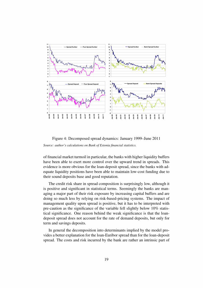
The estimated pure spread dynamics follows a broadly similar line withthe observed interest spreads and are correlated to the degree of 87% with theloan-Euribor spread and 69% for the loan-deposit spread (see Figure 4). Ascan be seen from the error correction model (see Table 3 in Appendix) thelending spread over Euribor is more sensitive to the Euribor volatility as wellas to market competition. Fierce competition in the credit market becomesevident in a negative market structure coefficient and in a lower pure spreadrelative to the deposit spread.27 The strongest pressure on loan rates can beobserved at the end of the loan boom in 2006–2007, when the rates becamesubstantially suppressed.
Interest rate volatility has a relatively small nominal effect on both spreads.This evidence can be explained by the fact that a large share of the Estonianbanks’ loan portfolio has a flexible-Euribor pegged loan rate which is reviewedevery six months. Even so it is noticeable that the interest rate volatility in thecomposition of the spread has gained weight at times when there is an upwardtrend in the average Euribor rate. The major determinant of the pure spreadis the risk aversion of the banking sector, which has significantly widened thespreads since the eruption of the global financial crisis in late 2007.
The analysis has also revealed a few factors that narrow the observed spread.Firstly, a higher share of foreign ownership in bank capital leads to a cut inspreads (see Table 2 and Figure 5). Equally, the strong liquidity position en-ables the banks to offer more favourable rates to their customers. During times
27The negative coefficients for market structure have earlier been reported by Saunders andSchumacher (2000) for the banking sectors in France and the UK, which appeared to be morecompetitive than Germany, Spain, Italy, Switzerland or the USA.
18
-1
0
1
2
3
4
5
6
7
8
9
10
11
Spread Euribor Pure Spread Euribor
0
1
2
3
4
5
6
7
8
Ja
n-9
9
Ja
n-0
0
Ja
n-0
1
Ja
n-0
2
Ja
n-0
3
Ja
n-0
4
Ja
n-0
5
Ja
n-0
6
Ja
n-0
7
Ja
n-0
8
Ja
n-0
9
Ja
n-1
0
Ja
n-1
1
Spread Deposit Pure Spread Deposit
-1
0
1
2
3
4
5
6
7
8
9
10
11
Spread Euribor Bank Spread Euribor
-2
-1
0
1
2
3
4
5
6
7
8
Ja
n-9
9
Ja
n-0
0
Ja
n-0
1
Ja
n-0
2
Ja
n-0
3
Ja
n-0
4
Ja
n-0
5
Ja
n-0
6
Ja
n-0
7
Ja
n-0
8
Ja
n-0
9
Ja
n-1
0
Ja
n-1
1
Spread Deposit Bank Spread Deposits
Figure 4: Decomposed spread dynamics: January 1999–June 2011
Source: author’s calculations on Bank of Estonia financial statistics.
of financial market turmoil in particular, the banks with higher liquidity buffershave been able to exert more control over the upward trend in spreads. Thisevidence is more obvious for the loan-deposit spread, since the banks with ad-equate liquidity positions have been able to maintain low-cost funding due totheir sound deposits base and good reputation.
The credit risk share in spread composition is surprisingly low, although itis positive and significant in statistical terms. Seemingly the banks are man-aging a major part of their risk exposure by increasing capital buffers and aredoing so much less by relying on risk-based-pricing systems. The impact ofmanagement quality upon spread is positive, but it has to be interpreted withpre-caution as the significance of the variable fell slightly below 10% statis-tical significance. One reason behind the weak significance is that the loan-deposit spread does not account for the rate of demand deposits, but only forterm and savings deposits.
In general the decomposition into determinants implied by the model pro-vides a better explanation for the loan-Euribor spread than for the loan-depositspread. The costs and risk incurred by the bank are rather an intrinsic part of
19

Table 2: I-Step: GLS panel estimation, December 1998–June 2011
Observed spread w.r.t Deposit rate Euribor 6M
Inverse efficiency 0.8062* 1.3270***(0.4653) (0.4473)
Liquidity –0.0366*** –0.0217*(0.0133) (0.0130)
Credit risk 0.0092* 0.0106**(0.0054) (0.0052)
Management quality 0.0168 0.0153(0.0109) (0.0106)
Foreign ownership in capital –0.0182*** –0.0147**(0.0067) (0.0063)
Net fees to assets 4.2872*** 4.8534***(0.8468) (0.8337)
Deposit quarantee costs 11.9379 20.1292**(8.9595) (8.7880)
Not foreign affiliate 1.1637** 1.2629**(0.5930) (0.5540)
Consumer credit 4.4576*** 4.4843***(0.7096) (0.7312)
Corporate long 0.4049 0.5723(0.5139) (0.5526)
Corporate short 0.5187 0.6584(0.4958) (0.5295)
Bank dummies YES YESPure spread dummies YES YES
Wald Chi2 650.35 933.69No of obs. 2871 2871
Source: author’s calculations on Bank of Estonia financial statistics.Note: Standard errors adjusted for panel-specific AR1 autocorrelation structure. ***, **, *indicate statistical significance at the 1%, 5% and 10% levels respectively.
20

PURE LOAN-DEPOSIT SPREAD
0
1
2
3
4
5
PURE LOAN-EURIBOR SPREAD
-3
-2
-1
0
1
2
3
4
5
1999 2000 2001 2002 2003 2004 2005 2006 2007 2008 2009 2010 2011
Market Structure and trend Volatility Risk Aversion Pure Spread
LOAN-EURIBOR SPREAD
-2
0
2
4
6
8
10
12
1999 2000 2001 2002 2003 2004 2005 2006 2007 2008 2009 2010 2011
Pure Spread Costs Regulation Bank-portfolio effects
Credit Risk Foreign ownership Liquidity Management
EURIBOR Total Spread
LOAN-DEPOSIT SPREAD
-2
0
2
4
6
8
10
12
Figure 5: Decomposed spread structure: January 1999-June 2011, year aver-ages
Source: author’s calculations on Bank of Estonia financial statistics.
the lending rate, whereas the deposit rate is more dependent on access and thecosts of liquidity.
In the light of the global financial crisis, the pure spread equations have alsobeen run for the period 2007–2011, in order to control for whether the effectswork in the same direction. The long term coefficients for risk aversion andinterest volatility have retained the expected signs and are highly statisticallysignificant. The market structure term has become more negative, reflectingthe increased competition over recent years. The interest rate volatility coeffi-cients became substantially larger relative to their value over the total period.Risk-aversion has also gained a greater role in explaining the long-term equi-librium of the spread. In general the results confirmed that the model for thecrisis period provided coefficients along the expected lines, revealing height-ened competition in the banking market in the years 2007–2011 despite highersensitivity to risks and volatilities.
21

8. Summary
In the aftermath of the global financial crisis the bank interest spreads inEstonia have reached their highest levels for a decade. The current researchaims to explain the determinants of the interest spreads in order to cast lighton the reasons behind the sudden surge in the bankers’ mark-up.
Employing the Ho and Saunders (1981) pure interest spread concept andthe two-step estimation procedure, the interest spreads have been decomposedinto sector- and bank-level determinants. It follows that the model provides abetter explanation for the loan-Euribor spread than for the loan-deposit spread.The costs and risks incurred by the bank are an intrinsic part of the lending rate,whereas the deposit rate is more dependent on access and the costs of liquidityon money markets.
The evidence proves that the credit market in Estonia is very competitive.The strongest pressure on loan rates can be observed at the end of the lendingboom in 2006–2007, when the rates became substantially suppressed. Therehas however been some room for banks to exert their market power in thedeposit market.
The risk-aversion of the sector is one of the main triggers behind the widen-ing spreads, and even more so since the eruption of the recent global financialcrisis. The banks keep holding strong capital positions over their risk expo-sures.
The interest rate volatility, though statistically significant, has a relativelymodest share in the spread composition. The banks have largely transferredthe interest rate risk to borrowers by imposing flexible Euribor-linked rate con-tracts.
The bank-specific spread is composed of the regulatory, efficiency and bankportfolio effects, each of which has a roughly equal weight in the observedspread, while credit risk adds only a tiny portion to the mark-up. Strong liq-uidity and foreign capital have enabled the banks to counteract and alleviatesome of the upward trend in the spreads.
The overall implication suggests that in spite of the improved efficiency,the competitive market and dominant foreign participation, the banks’ spreadsin Estonia remain vulnerable to global risks, being increased by the heightenedrisk-aversion of banks at times of high uncertainty.
22

References
ALLEN, L. (1988): “The Determinants of Bank Interest Margins: A Note,”Journal of Financial and Quantitative Analysis, 23(02), 231–235.
ANGBAZO, L. (1997): “Commercial bank net interest margins, default risk,interest-rate risk, and off-balance sheet banking,” Journal of Banking& Finance, 21(1), 55–87.
BANERJEE, A., J. DOLADO, J. GALBRAITH, AND D. HENDRY (1993): Co-integration, error-correction, and the econometric analysis on non-stationary data. Oxford University Press.
BECK, N., AND J. N. KATZ (1995): “What to do (and not to do) with Time-Series Cross-Section Data,” The Ametical Political Science Review, 89,634–647.
CHEN, X., S. LIN, AND W. R. REED (2006): “Another Look at what to dowith Time-series Cross-section Data,” Working papers in economics,University of Canterbury, Department of Economics and Finance.
CLAEYS, S., AND R. VANDER VENNET (2008): “Determinants of bank in-terest margins in Central and Eastern Europe: A comparison with theWest,” Economic Systems, 32(2), 197–216.
DRAKOS, K. (2003): “Assessing the success of reform in transition banking10 years later: an interest margins analysis,” Journal of Policy Model-ing, 25(3), 309–317.
HAWTREY, K., AND H. LIANG (2008): “Bank interest margins in OECDcountries,” The North American Journal of Economics and Finance,19(3), 249–260.
HO, T. S. Y., AND A. SAUNDERS (1981): “The Determinants of Bank InterestMargins: Theory and Empirical Evidence,” Journal of Financial andQuantitative Analysis, 16(04), 581–600.
KATTAI, R. (2010): “Credit risk model for the Estonian banking sector,” Bankof Estonia Working Papers Working Paper 2010-01, Bank of Estonia.
KIT, P. W. (1997): “On the determinants of bank interest margins under creditand interest rate risks,” Journal of Banking & Finance, 21(2), 251–271.
MAUDOS, J., AND J. FERNANDEZ DE GUEVARA (2004): “Factors explain-ing the interest margin in the banking sectors of the European Union,”Journal of Banking & Finance, 28(9), 2259–2281.
23

PODESTA, F. (2000): “Recent Development in Quantitative ComparativeMethodology: the Case of Pooled Time Series Cross-Section Analy-sis,” Discussion paper, Georgetown University.
POGHOSYAN, T. (2010): “Re-examining the impact of foreign bank partic-ipation on interest margins in emerging markets,” Emerging MarketsReview, 11(4), 390–403.
SAUNDERS, A., AND L. SCHUMACHER (2000): “The determinants of bankinterest rate margins: an international study,” Journal of InternationalMoney and Finance, 19(6), 813–832.
WOOLDRIDGE, J. M. (2002, 2010): Econometric analysis of cross sectionand panel data. The MIT Press.
24

9. Appendixes
Table 3: II-Step: Error Correction Model, January 1999–June 2011
Pure Spread w.r.t Deposit rate Euribor 6 months1999-2011 2007-2011 1999-2011 2007-2011
dVolatility 0.8243*** 0.6049 1.0295*** 2.1475***(0.2171) (0.3975) (0.3822) (0.5750)
dRisk-aversion 0.0589** 0.0761*** 0.0619* 0.1051***(0.0295) (0.0225) (0.0329) (0.0354)
Adjustment –0.3173*** –0.1593*** –0.1507*** –0.1275***(0.0626) (0.0589) (0.0336) (0.0423)
LVolatility 1.1201*** 1.5625*** 1.3881*** 3.7090***(0.3561) (0.4829) (0.4425) (0.3260)
LRisk-aversion 0.0775*** 0.0513** 0.0563*** 0.0646***(0.0196) (0.0204) (0.0175) (0.0161)
LnTrend –0.1540* –0.0960*(0.0781) (0.0560)
Market structure 0.3155 -0.5138** –0.4191** –1.2146***(0.2808) (0.2510) (0.1977) (0.2465)
F 9.69 5.05 6.11 34.62No of obs. 150 54 150 54R square 0.21 0.26 0.19 0.63R square adj 0.18 0.19 0.16 0.59
LONG-RUN EQUILIBRIUM 1999-2011:
SpreadDeposits = 0.99− 0.49LnT + 3.53V + 0.24RA
SpreadEuribor = −2.78− 0.64LnT + 9.21V + 0.37RA
LONG-RUN EQUILIBRIUM 2007-2011:
SpreadDeposits = −3.23 + 9.81V + 0.32RA
SpreadEuribor = −9.52 + 29.09V + 0.51RA
Source: author’s calculations on Bank of Estonia financial statistics.Note: Robust standard errors in parentheses. ***, **, * indicate statistical significance at thelevels of 1%, 5% and 10% respectively.
25

Table 4: II-Step: ECM with period effects, January 1999-June 2011
Pure Spread w.r.t Deposit rate Euribor 6 monthsannual effects 3-year effects annual effects 3-year effects
dVolatility 0.5436** 0.9390*** 0.9732** 1.1325***(0.2561) (0.2307) (0.4661) (0.4106)
dRisk-aversion 0.0577 0.0791** 0.0463 0.0737**(0.0424) (0.0342) (0.0426) (0.0358)
Adjustment –0.4980*** –0.3854*** –0.2677*** –0.2221***(0.0852) (0.0656) (0.0808) (0.0551)
LVolatility 0.8921** 1.4555*** 1.4121*** 1.6692***(0.3745) (0.3294) (0.5276) (0.4391)
LRisk-aversion 0.0564 0.1064*** 0.0324 0.0604**(0.0480) (0.0281) (0.0488) (0.0244)
2000 –0.7838*** –0.8133**(0.2609) (0.3654)
2001 –0.6128** –0.8880**(0.2641) (0.3686)
2002 –0.5941** –0.8296**(0.2318) (0.3711)
2003 –0.5573** –0.7097**(0.2406) (0.3284)
2004 –0.6624** –0.7551**(0.2922) (0.3586)
2005 –0.9629*** –0.7922**(0.3178) (0.3982)
2006 –0.8895*** –0.9678***(0.2861) (0.3527)
2007 –1.2936*** –1.1826***(0.3220) (0.4313)
2008 –0.7401*** –0.8059*(0.2603) (0.4136)
2009 –0.7790** –0.3493(0.3758) (0.3180)
2010 –0.5110 –0.5962(0.3681) (0.4201)
2011 –0.3522 –0.6928(0.3509) (0.4366)
2000–2002 –0.4360** –0.6275**(0.2162) (0.2809)
2003–2005 –0.4169* –0.5054*(0.2270) (0.2751)
2006–2008 –0.6977*** –0.7556**(0.2386) (0.3000)
2009–2011 –0.7647*** –0.5570**(0.2755) (0.2318)
constant 1.3283* –0.0599 0.4958 –0.2150(0.7660) (0.4034) (0.8177) (0.4854)
F 5.23 6.76 2.90 4.14No of obs. 150 150 150 150R square 0.32 0.25 0.27 0.24R square adj 0.23 0.20 0.18 0.19
Source: author’s calculations on Bank of Estonia financial statistics.Note: Robust standard errors in parentheses. ***, **, * indicate statistical significance at thelevels of 1%, 5% and 10% respectively.
26

Working Papers of Eesti Pank 2011
No 1Jaanika MeriküllLabour Market Mobility During a Recession: the Case of Estonia
No 2Jaan Masso, Jaanika Meriküll, Priit VahterGross Profit Taxation Versus Distributed Profit Taxation and Firm Performance: Effects of Estonia’s Corporate Income Tax Reform
No 3Karin Kondor, Karsten StaehrThe Impact of the Global Financial Crisis on Output Performance Across the European Union: Vulnerability and Resilience No 4Tairi Rõõm, Aurelijus DabušinskasHow Wages Respond to Shocks: Asymmetry in the Speed of Adjustment
No 5Kadri Männasoo and Jaanika MeriküllR&D, Demand Fluctuations and Credit Constraints: Comparative Evidence from Europe
No 6Aurelijus Dabušinskas, Tairi RõõmSurvey Evidence on Wage and Price Setting in Estonia
No 7Kadri Männasoo and Jaanika MeriküllR&D in boom and bust: Evidence from the World Bank Financial Crisis Survey
No 8Juan Carlos Cuestas, Karsten StaehrFiscal Shocks and Budget Balance Persistence in the EU countries from Central and Eastern Europe
No 9Kadri Männasoo, Jaanika MeriküllHow Do Demand Fluctuations and Credit Constraints Affect R&D? Evidence from Central, Southern and Eastern Europe
No 10Martti Randveer, Lenno Uusküla, Liina KuluThe Impact Of Private Debt On Economic Growth


