Accepted Manuscript Determinants of Renewable Energy Growth in Sub-Saharan Africa: Evidence from Panel ARDL Patrícia Pereira da Silva, Pedro André Cerqueira, Wojolomi Ogbe PII: S0360-5442(18)30888-0 DOI: 10.1016/j.energy.2018.05.068 Reference: EGY 12903 To appear in: Energy Received Date: 02 September 2017 Revised Date: 29 April 2018 Accepted Date: 09 May 2018 Please cite this article as: Patrícia Pereira da Silva, Pedro André Cerqueira, Wojolomi Ogbe, Determinants of Renewable Energy Growth in Sub-Saharan Africa: Evidence from Panel ARDL, (2018), doi: 10.1016/j.energy.2018.05.068 Energy This is a PDF file of an unedited manuscript that has been accepted for publication. As a service to our customers we are providing this early version of the manuscript. The manuscript will undergo copyediting, typesetting, and review of the resulting proof before it is published in its final form. Please note that during the production process errors may be discovered which could affect the content, and all legal disclaimers that apply to the journal pertain.
Transcript
Accepted Manuscript
Determinants of Renewable Energy Growth in Sub-Saharan Africa: Evidence from Panel ARDL
Patrícia Pereira da Silva, Pedro André Cerqueira, Wojolomi Ogbe
PII: S0360-5442(18)30888-0
DOI: 10.1016/j.energy.2018.05.068
Reference: EGY 12903
To appear in: Energy
Received Date: 02 September 2017
Revised Date: 29 April 2018
Accepted Date: 09 May 2018
Please cite this article as: Patrícia Pereira da Silva, Pedro André Cerqueira, Wojolomi Ogbe, Determinants of Renewable Energy Growth in Sub-Saharan Africa: Evidence from Panel ARDL,
(2018), doi: 10.1016/j.energy.2018.05.068Energy
This is a PDF file of an unedited manuscript that has been accepted for publication. As a service to our customers we are providing this early version of the manuscript. The manuscript will undergo copyediting, typesetting, and review of the resulting proof before it is published in its final form. Please note that during the production process errors may be discovered which could affect the content, and all legal disclaimers that apply to the journal pertain.
ACCEPTED MANUSCRIPT
1
DETERMINANTS OF RENEWABLE ENERGY GROWTH IN SUB-SAHARAN AFRICA: EVIDENCE FROM PANEL ARDL
Given the importance of renewable energy in the discussion of a reliable and sustainable energy future, it is imperative to understand its main determinants and to draw result implications for energy policy. This study analyses these determinants for Sub-Saharan Africa. Using a panel data technique, namely the panel-ARDL model for a period covering 1990-2014, the results suggest that economic development (per capita GDP) and an increased use of energy aid renewable energy development while population growth impedes it. Furthermore, the study investigates the potentials and current status of renewable energy in Sub-Saharan Africa. This article shows that although the region has great potential for developing renewable energy such as wind, biomass, solar and hydropower, dispersed throughout the continent, this potential has not been fully explored, even though many resources are plentifully available, and evidence good economic potential.
1. INTRODUCTION
Renewable energy (RE) plays an important role in meeting the needs of a country in terms of sustainable development. The development and proper use of renewable energy should be given high priority, especially with the current environmental issues of climate change and global warming being in the forefront among the most critical energy related issues in the world today. The increased attention on renewable energy sources (RES) can be attributed to a number of factors beyond climate change. The recent concerns over the volatility of oil prices and the dependency on foreign energy sources are all contributing factors to the current interest in RES (Apergis & Payne , 2010). Encouraged by this increasing importance, utilization of RES has experienced a remarkable global growth profile in recent times (Aguirre & Ibikunle, 2014). Given this important role of RES in the discussion of a reliable and sustainable energy future, as can be drawn from the previous discussions, it is important to understand its main determinants and to draw result implications for energy policy. Marques et al. (2010) highlighted some important determining factors in the deployment of renewable sources to include political, socioeconomic and country-specific factors.
In this context, Sub-Saharan Africa (SSA) presents great energy resources and has great potential for developing RE such as wind, biomass, solar and hydro power, dispersed across regions, which makes it an attractive place for REs investors. However, inadequate electricity generation remains an issue (Suberu et al., 2013; Aliyu et al., 2018). The development of the RE sector has the potential of limiting harmful emissions, providing sufficient electricity for its teeming population and also promoting sustainable development objectives.
A number of studies have been carried out mentioning the RE potential of SSA countries (Eberhard et al., 2011; Prasad, 2011; Bazilian, et al., 2012; Suberu et al., 2013; IEA, 2014; Mukasa et al.,
ACCEPTED MANUSCRIPT
2
2015; Adams et al., 2016; Rupf et al., 2016), but there is a lack of in-depth empirical studies carried out to analyse the drivers of RE in these countries. This article aims to bridge that gap by performing an empirical analysis to determine the factors that affect the growth of RE in SSA countries. The share of RES in the electricity mix is used as the proxy to measure RES growth. The specific research question addressing the determining factors which aid or hinder the growth of Renewable Energy in SSA.
The next section develops a literature review of previous studies that deal with RE growth and its determinants. Section 3 embodies the specificities of energy development in SSA. The fourth section provides the overall methodology employing the panel-ARDL methodology in the econometric analysis followed by the discussion of the result and findings of the research. Section 5 concludes and recaps the key findings of the research and future work is also suggested.
2. DETERMINANTS OF RENEWABLE ENERGY GROWTH – PREVIOUS WORKS
The increased attention on RE sources can be attributed to a number of factors such as the concerns over the volatility of oil prices, the dependency on foreign energy sources, and the environmental consequences of carbon emissions (Apergis & Payne , 2010). This section performs a review of the underlying influences as regards the factors, which drive RE growth. As is mentioned by Marques et al., (2010) and Aguirre & Ibikunle (2014), the important factors which drive or determine RE deployment can be split into political, socio-economic and country specific factors.
2.1. Political Factors
Several studies, such as those carried out by Carley (2009), Marques & Fuinhas (2012) and Kilinc-Ata (2016) pointed out political motivations as the most relevant aspect to the promotion of RE. Political factors that influence RE growth include public policies, institutional variables and energy security.
As Aguirre & Ibikunle (2014) stated, RE technologies are relatively expensive and cannot compete with traditional energy technologies without supporting policies. In this set up, several studies (Marques & Fuinhas, 2012; Maria & Bernauer, 2014; Stadelmann & Castro, 2014; Kilinc-Ata, 2016) discussed how public policies are one of the major motivating factors of RE growth. Some of the most common public policy measures to encourage renewables include subsidies, quota policies, direct investment, research and development, feed-in tariffs, and green certificates. Polzin et al. (2015) highlighted the importance of establishing reliable frameworks and long-term policy objectives on the growth of RE but revealed that these have to be technology-specific. Those frameworks could be influenced by both domestic and international factors such as characteristics of domestic political institutions or by what other countries, or group of countries (e.g. the European Union) (Maria & Bernauer, 2014; Stadelmann & Castro, 2014). Accordingly, policy design features tend to vary in structure, size, application, eligibility, and administration (Wiser et al., 2007). Despite these variations, public policies are aimed at increasing the capacity or percentage of RE.
Following Carley (2009), institutions frame the way political actors operate, and both directly and indirectly shape the structure of policy outcomes. The capacity of political organizations, the ideological underpinnings of political actors, and inter-party competition all affect the likelihood of
ACCEPTED MANUSCRIPT
3
environmental policy adoption and the degree to which outcomes conform to the policy objectives. The adoption of the Kyoto-Protocol in 1997 was one of the earlier global measures put in place to tackle the environmental problems plaguing the world. The goal of the Kyoto-Protocol was to commit countries into reducing GHG emissions and to increase the share of electricity produced from renewables. Such commitments to reduce emissions and increase share of renewables is one of the driving factors for the growth of renewables in countries (Pablo, 2005; Popp et al., 2011). Furthermore, global or regional institutions like the United Nations, European Union or the African Union set targets regarding emissions reduction and renewables deployment. Countries that are members of such institutions are thus incentivised to increase their shares of RE.
Also, a country’s energy security is important and domestic RE deployment contributes to its improvement related to geographic diversification and energy dependence. If RES are deployed at a national level, they reduce energy dependence and the vulnerability entailed by the concentration of energy sources and origins (Escribano Francés et al., 2013; Augutis et al., 2014; Lucas et al., 2016).
Literature supports the hypothesis that energy security advances renewables deployment (Gan et al., 2007; Chien & Hu, 2008). Chien & Hu (2008) suggested that the import substitution of traditional energy by locally produced renewables has direct and indirect effects on increasing an economy’s trade balance and the country’s energy security. The higher the reliance of a country on energy imports, the higher the level of renewables deployment required in order to improve that country's energy security (Aguirre & Ibikunle, 2014).
2.2. Socioeconomic Factors
Socioeconomic factors of RE deployment include CO2 emissions, prices of conventional energy sources, country gross domestic product (GDP) and energy demand.
Of the main greenhouse gases emitted into the atmosphere, CO2 has the highest share and as such, the reduction of CO2 emissions is a foremost objective for achieving sustainability (Rüstemoglu & Andrés , 2016). The literature is plentiful with discussions on the impacts of CO2 and its role in fostering the development of RE (Sardosky, 2009a; Marques et al., 2010; Aguirre & Ibikunle, 2014; Omri & Khuong, 2014; Rafiq et. al, 2014). Sardosky (2009a) suggested that increases in carbon dioxide emissions, are a major driver to increased deployment of RE. Marques et al. (2010) also highlighted that CO2 emissions are significant indicators of renewable deployment, a view shared by Aguirre & Ibikunle (2014). However, they went on to suggest that carbon dioxide emission has a negative relationship with RE deployment which means that it did not promote the development of RE, which is a surprising result. Increases in carbon dioxide emissions, coupled with increased concern over global warming, are likely to lead to increased consumption of RE (Sadorsky, 2009a).
Energy consumption is traditionally used as a development indicator. It is also used to reveal the energy needs of a country. Larger consumption needs, exert strong pressure on the level of energy use. The energy consumption could be supplied by traditional energy sources, by renewables, and by using a combination of traditional and renewables (Marques et al., 2010). Population and population growth are further indicators of the energy needs of a country. The projections of the International Energy Agency (IEA, 2015) indicated that energy demand is expected to increase considerably in the coming years as the result of population growth and economic development
ACCEPTED MANUSCRIPT
4
driven primarily by Asian and African countries. In 2014, 63% of Sub-Saharan Africa's population still had no access to electricity. This implies that there is a need to provide modern energy to the present generation and make plans to accommodate for the future ones (Ackah & Kizys, 2015; WB, 2018). Carley (2009) suggested that countries with larger growth rates would likely build more power capacity to satisfy growing demand for electricity with RE deployment being a viable option for satisfying this rising demand. However, Aguirre & Ibikunle (2014) imply that energy use is negatively linked to RE participation, stating that under high pressure to ensure the energy supply, countries with increasing energy requirements are inclined to pursue more fossil fuel solutions and other cheap alternatives instead of renewables to cover electricity demand. This view is shared by Pfeiffer & Mulder (2013) who suggested that growth of electricity consumption appears to delay RE diffusion.
The prices of alternate energy sources, in this case fossil fuels, also play an important role in determining the use of RE. The prices of RES have been falling and are at par, and in some cases, even cheaper than traditional sources (IRENA, 2018). However, the prices of traditional energy sources fail to reflect the real costs of their use, when compared to those of RE considering the environmental costs are not taken into account (Menz & Vachon, 2006; Marques et al., 2010; Foster et al., 2017); anthropogenic greenhouse gas emissions are increasing at a rapid rate and are very likely to be already causing changes to the global climate system (IPCC, 2014). Yet, as Abas et al. (2015) pointed out, new global investments in oil and gas sector increased from 2004 to 2011 but started declining again after 2012, and the recent plunge in oil prices has discouraged investment in oil and gas exploration which could potentially have an effect of increased development of renewables. Bird et al. (2005), in their study on market factors driving wind power development in the United States, suggested that the increasing cost-competitiveness of wind generated electricity attributable to high natural gas prices is an important driver for new wind installations. Van Ruijven & Van Vuuren (2009) examined the interaction of renewables and hydrocarbon prices in high and low GHG emission mitigation scenarios. Their results followed up on Bird et al. (2005) by opining that with high hydrocarbon prices, there is an improved position of RES. However, Sadorsky (2009a) contradicted this by suggesting that oil price increases have a smaller although negative impact on RE consumption; a view shared by Omri & Khuong (2014). The results of Van Ruijven & Van Vuuren (2009) were further corroborated by Reboredo (2015), who concluded that high oil prices encourage development of the RE sector since the economic viability of RE projects is enhanced, whereas low oil prices have the opposite effect.
Additionally, the wealth of a country, commonly measured by the GDP or the GDP per capita, plays a significant role in determining the employment of renewables. A higher level of income means a higher potential or more resources to foster RE growth. Larger income allows countries to handle the costs of developing RE technologies and guaranteeing higher support for the costs of public policies in promoting and regulating renewables. The relationship between economic growth and renewables deployment has been examined by a number of studies (Sadorsky, 2009a; Sadorsky, 2009b; Apergis & Payne, 2010; Menegaki, 2011; Ohler & Fetters, 2014) and there is somewhat of a consensus as to the how they affect each other. Sadorsky (2009a) showed that in the long term, an increase in real GDP per capita is found to be a major driver behind per capita RE consumption. Similarly, Sadorsky (2009b) concluded that increases in real per capita income affect significantly and positively per capita RE consumption, meaning that higher economic growth would require
ACCEPTED MANUSCRIPT
5
more RE as a share of the total energy consumption. Chang et al. (2009) improved on the study of Sadorsky (2009a, 2009b) by investigating the influence that energy prices have on RE development under different economic growth rate regimes for the OECD member-countries. The results suggested that countries with high rates of economic growth can respond to energy price impacts by changing their use of RE. On the other hand, countries with low rates of economic growth tend to be unresponsive to energy price changes in their RE use.
2.3. Country Specific Factors
Individual country specificities such as RE potentials and market regulations factor in as determinants of RE deployment. The natural endowment with RE resources, such as solar irradiation, waterfalls or strong winds plays a key role in renewables deployment. These resources need to be present in sufficient quantity and quality to make RE investments competitive (Bird, et al., 2005). In their studies, Carley (2009) and Aguirre & Ibikunle (2014) showed that solar, biomass and wind potential are statistically significant in explaining renewables growth suggesting that countries that have greater RE potential are expected to deploy more of these technologies. Stadelmann & Castro (2014) concluded that governments are more likely to support RE technologies if their countries have sufficient natural resources to make them work in the first place.
Furthermore, as Siddiqui et al. (2016) concluded, the structure of an energy market has significant effects on the deployment of renewables. Chassot et al. (2014) empirically demonstrated that venture capital investors exhibit policy risk aversion, in that they tend to avoid RE investment opportunities if regulatory exposure is perceived to be high. They showed that the aversion to policy risk is more pronounced among investors who hold strong individualistic worldviews and thus prefer “free markets” rather than government intervention. These views are different to that of Pfeiffer & Mulder (2013) who discovered that renewables diffusion accelerates with the implementation of economic and regulatory instruments. Nesta et al. (2014) found a significant effect of energy market liberalisation on innovation in RE technologies implying that, given the characteristics of the energy market, in which the core competences of the incumbent are generally tied to fossil fuel plants whereas the production of RE is mainly decentralised in small-sized units, the entry of non-utility generators made possible by market liberalisation increases the incentives for renewables.
2.4 Technological innovation
In their study on assessing the impact of technological change on investment in renewable energy, carried out with data across 26 OECD countries from 1991 to 2004, Popp et al. (2011) used the PATSTAT database to obtain a comprehensive list of patents for investment in wind, solar photovoltaic, geothermal, and electricity from biomass and waste. They found that technological advances do lead to greater investment, but the effect is small. Investments in other carbon-free energy sources, such as hydropower and nuclear power, serve as substitutes for renewable energy i.e. less investments in renewables. Kumar & Agarwala (2016) further pointed out that renewable energy technology diffusion rate is higher due to technological improvements resulting in cost reductions and government policies supportive of renewable energy development and utilization.
ACCEPTED MANUSCRIPT
6
3. ENERGY AND SUSTAINABILITY IN SUB-SAHARAN AFRICA
The population of SSA in 2014 was around 979 million people, with growth being rapid, having increased by 309 million people from 2000 to its 2013 figure, and it is expected to reach one billion well before 2020. This huge increase magnifies many existing challenges, such as the quest to achieve modern energy access. Population growth has been split relatively evenly between urban and rural areas, in contrast to the strong global trend to urbanisation. Only 37% of the SSA population lives in urban areas – one of the lowest shares of any world region – that has important implications for the approach to solving the energy challenges. (IEA, 2014).
Access to electricity is calamitous in SSA - there are more people living without access to electricity in SSA than in any other world region – more than 612 million people, and nearly half of the global total. It is also the only region in the world where the number of people living without electricity is increasing, as rapid population growth is outpacing the many positive efforts to provide access. As Adams et al. (2016) strengthened, the energy consumption of the average African in the early 2000s was less than what an average British used in England more than a hundred years ago. Overall, the electricity access rate for SSA has improved from 23% in 2000 to 37% in 2014 with the electrification levels ranging from 3% in Burundi to 100% in Mauritius — the only country in SSA that has achieved 100% electrification (Prasad, 2011). In comparison, more than 99% of the total population of North Africa has access to electricity. Nearly 80% of those lacking access to electricity across SSA are in rural areas. For those that do have electricity access in SSA, average residential electricity consumption per capita is 317 kWh per year (225 kWh excluding South Africa) (IEA, 2014). Eberhard et al. (2011) noted that installed capacity will need to grow by more than 10 percent annually just to meet Africa’s suppressed demand, keep pace with projected economic growth, and provide additional capacity to support efforts to expand electrification.
Grid-based power generation capacity has increased from around 68 GW in 2000 to 99 GW in 2014, with South Africa alone accounting for about half of the total. Coal-fired generation capacity is 45%, followed by hydropower (22%), oil-fired (17%), gas-fired (14%), nuclear (2%) and other renewables (less than 1%). Until recently, countries developed their power systems largely independently of one another, focusing on domestic resources and markets, but there has been progress towards regional co-operation to permit concentrated resources, such as large hydropower, to serve larger markets (IEA, 2014). In addition to capacity linked to the main grid, there has been increasing emphasis on developing mini-grids and off-grid systems. To further supplement their power supply, many individuals and businesses have access to small diesel or gasoline-fuelled generators
RE technologies (mainly hydropower) make up a large share of total power supply in Africa and there is potential for this to expand as a wider range of technologies is deployed. Many countries are actively developing, or considering developing, their RE resource potential. Suberu et al. (2013) highlighted that modern RE development in SSA is lagging behind many any other regions in the world due to a number of reasons such as limited capital investment, lack of technological knowledge on RE development, unreliable equipment, low rate of electrification and high transmission losses.
ACCEPTED MANUSCRIPT
7
3.1 Hydropower
Hydropower has long been an important part of many African power systems and is the mostly used RE source. Eberhard et al. (2011) report that over 900 TWh (about 220 GW installed capacity) of viable hydropower potential in SSA remains unexploited, located primarily in the Democratic Republic of Congo, Ethiopia, Cameroon, Angola, Madagascar, Gabon, Mozambique, and Nigeria. Similarly, the Intergovernmental Panel on Climate Change (IPCC) estimates the technical hydropower potential at 1174 TWh per year (or 283 GW of installed capacity). This amount of electricity is more than three-times the current electricity consumption in SSA. So far, less than 10% of the technical potential has been tapped into (Bazilian et al., 2011; IEA, 2014).
3.2 Solar Power
Africa is particularly rich in solar energy potential, with most of the continent enjoying an average of more than 320 days per year of bright sunlight and irradiance levels of almost 2000 kWh per square metre annually (IEA, 2014).
Yet, solar technologies have played a limited role in the power sector in Africa, but are gaining attention in many countries. As Suberu et al. (2013) noted, solar energy consumption is currently limited to lighting and the operation of simple appliances in both rural and urban areas of SSA. Solar-powered water heaters, solar-powered cookers, building integrated photovoltaics and the application of solar photovoltaic distributed electric power generation are limited to just a few countries in SSA. They are more common in countries such as South Africa and Mauritius where there is an increasing tendency to embrace emerging RE technologies in line with the accelerated global pace of Renewable Energy consumption.
Solar energy is gaining a foothold in SSA where installed capacity increased from 40 MW in 2010 (mainly small-scale PV) to around 280 MW in 2013 (including some large PV and concentrating solar power plants). There are several grid-connected projects under construction, including the 155 MW Nzema plant in Ghana and 150 MW of projects in South Africa. In addition, other countries are considering projects on the scale of 100 MW or more, including Mozambique, Sudan, Nigeria and Ethiopia (IEA, 2014).
3.3 Wind Power
Wind power deployment in SSA to date has been very limited when compared to hydropower, even though the levelised cost of electricity from onshore wind technologies has declined significantly in recent years. SSA’s wind potential is estimated at around 1300 GW (IEA, 2014). The IEA report further outlines that high quality wind resources are confined to a few areas, mainly the Horn of Africa, eastern Kenya, parts of West and Central Africa bordering the Sahara and parts of Southern Africa. Eight African countries are among the developing world’s most endowed with wind energy potential (Mukasa et al., 2015). Somalia has the highest onshore potential of any country, followed by Sudan, Libya, Mauritania, Egypt, Madagascar and Kenya. The offshore wind energy potential is best off the coast of Madagascar, Mozambique, Tanzania, Angola and South Africa (IEA, 2014).
ACCEPTED MANUSCRIPT
8
Despite this great potential supply of wind energy, installed capacity of wind-based electricity in SSA stands at only 190 MW (IEA, 2014).
3.4 Geothermal
Geothermal technologies make up a small fraction of Africa’s power supply, but adequate resources exist. These resources are concentrated in the East African Rift Valley, which is considered one of the most exciting prospects in the world for geothermal development, with total potential estimated at between 10 GW and 15 GW - more than East Africa’s total existing power generation capacity, a large share of which is concentrated in Ethiopia and Kenya. Kenya has around 250 MW of installed geothermal capacity and a further 280 MW is under development. More than 40 wells a year are currently being drilled in Kenya, and the target is to develop more than 5000 MW by 2030 which is about half of the estimated potential (IEA, 2014; Suberu et al., 2013). Ethiopia is also actively developing its geothermal resources that aim to add 1GW of capacity over the next decade. Several other countries are exploring their geothermal potential, but projects are challenging and typically have long-lead times. Zambia has a number of sites planned, while Tanzania is carrying out exploration (and has potential of around 650 MW), and Eritrea, Djibouti, Rwanda and Uganda have also carried out geothermal exploration (IEA, 2014).
3.5 Biomass
Estimates indicate that between 80% and 90% of the people in SSA depend on biomass fuels, and fuelwood accounts for more than 75% of the household energy balance (Jumbe et al., 2009). Varieties of biomass residues from agriculture, municipal solid waste and forest biomass can be found in sustainable quantities in SSA. Biomass for electricity generation has not been widely exploited in most regions in Africa, except South Africa and Mauritius, both of which use sugar cane in combustion power plants. The World Bank in its “Low Carbon Report”, while firmly advocating the use of solar PV, also suggested “other sources of power include using municipal waste to generate methane to generate power, combusting other biomass to make power, and small-scale hydropower. (…)”(WB, 2013: 91). Biomass consumption in Africa has traditionally been dominated by direct burning of bio residues for heat energy production, especially for cooking and heating purposes (Suberu et al., 2013).
Biogas, which is mainly obtained from varieties of biodegradable waste raw materials, is another promising clean source of energy for cooking and small power generation in rural districts. Although biogas is mainly used for cooking in developing countries, in developed nations it is used for both cooking and power generation. Some ongoing Renewable Energy programmes in the SSA region are actively advocating for biogas consumption for cooking. Different countries in SSA have attempted testing various bioelectricity conversion technologies, such as combustion, gasification and pyrolysis, although these are on a very small scale and at an experimental stage (Suberu et al., 2013). The total methane production potential from the feedstocks available to households, communities and at a commercial scale in SSA (excluding Sudan and South Sudan) is estimated to be 26.1 billion m3, equivalent to 270 TWh of heat energy. Crop waste normally burned makes up the greatest portion of this potential (36%), and also presents the greatest potential on a per capita basis. Benin is estimated to have the highest per capita energy production potential of 732 kWh/pp/yr with particularly high
ACCEPTED MANUSCRIPT
9
potentials for using crop waste normally burned and crop primary equivalent waste (CPEW) as biogas feedstocks. Ghana has the highest energy production potential from CPEW of 375 kWh/pp/yr (Rupf et al., 2016).
4. DETERMINING THE FACTORS BEHIND RENEWABLE ENERGY GROWTH IN SSA.
The main objective of this study is to carry out an analysis to determine the main determinants of RE growth in Sub-Saharan Africa, controlling for drivers already suggested by previous literature (Marques et al., 2010; Aguirre & Ibikunle, 2014).
4.1 DataWe use annual data for 17 Sub-Saharan countries - Nigeria, Benin, Congo Republic, Cameroon, Cote d’Ivoire, Ethiopia, Gabon, Ghana, Kenya, Mozambique, Namibia, Tanzania, Togo, Senegal, South Africa, Zambia and Zimbabwe - spanning 25 years from 1990 through 2014. Only 17 countries were used in the analysis due to a lack of recent and complete data for the rest of the Sub-Saharan countries. Furthermore, the period of study goes only until 2014 due to a lack of more recent data for the countries under analysis. Following Marques et al., (2010) and Aguirre & Ibikunle (2014), the explanatory variables are some of the drivers of RE in literature: CO2 emissions per capita, fossil fuel prices, population growth, GDP per capita, energy use, energy import and the ratification of the KYOTO protocol (represented as a dummy variable). All the variables except for the fossil fuel prices and the ratification of the KYOTO protocol were taken from the World Bank’s Development Indicators Database (WDI)1. The coal, oil and gas prices were retrieved from the British Petroleum’s statistical review of world energy (BP Stat.Rev.)2 and the year of ratification of the KYOTO protocol was taken from the United Nations Framework Convention on Climate Change (UNFCCC)3.
In Table 1, a summary of the variables used in the analysis, along with their descriptive statistics and data sources is presented.
The data sample is converted to a panel data format. Panel data contains more information, greater variability of data, less collinearity between the variables, higher number of degrees of freedom, and more efficiency in the estimates (Greene, 2003; Marques et al., 2010). CO2 emissions per capita, oil price, gas price, coal price, GDP per capita, energy use are converted to their natural logarithm format.
Table 1 - Variables definition and descriptive statistics
Variable name Definition Source Observations Mean Median Minimum Maximum Std. Dev.
Ren Share of Renewable Energy in electricity production (%)
World Data Bank 425 0.626 0.708 0 1 0.357
CoalPr Coal prices (US$ per tonne) BP Statistical Review of World Energy
25 59.954 43.6 28.79 147.67 30.634
GasPr Natural Gas prices (US$ per million Btu)
BP Statistical Review of World Energy
25 3.912 3.707 1.487 8.849 2.156
OilPr Crude Oil prices (US$ per barrel)
BP Statistical Review of World Energy
25 47.574 28.496 12.716 111.67 35.161
PopGr Population growth (%) World Data Bank 425 33.769 17.45 0.93 277.49 48.315
CO2pc CO2 emissions (metric tons per capita)
World Data Bank 425 1.06 0.322 0.017 10.024 2.124
GDPpc Gross domestic product per capita (constant 2010 US$)
World Data Bank 425 1929.351 965.11 161.83 11925.78 2604.321
Eneuse Energy Use (GWh/capita) World Data Bank 425 0.0078 0.0051 0.0024 0.036 0.0072
EneImp Share of Electricity Imports to Consumption (%)
World Data Bank 425 0.217 0.011 0 1.15 0.352
Kyoto Ratification of the Kyoto Protocol (DUMMY)
UNFCCC 425 0.428 0.00 0.00 1.00 0.495
ACCEPTED MANUSCRIPT
11
4.2 Methodology
Our panel sample has 17 countries and 25 years, and so has more years than cross-sample units, the variables might not be stationary but I(1) and the model is probably dynamic. In this framework the use of a panel-ARDL model as proposed by Pesaran and Smith (1995) and Pesaran et al. (1999) is more appropriate. According to these authors the advantages over other dynamic panel methods, such as the fixed effects, instrumental variables or the GMM estimators proposed by Anderson and Hsiao (1981, 1982), Arellano (1989), Arellano and Bover (1995) between others is that these methods can produce inconsistent estimates of the average value of the parameters unless the coefficients are identical across countries.
The model estimated has the form of an ARDL(p,q,q,…,q) model (Eq1):
Eq. 1𝑅𝑒𝑛𝑖𝑡 = ∑𝑝𝑗 = 1𝛼𝑖𝑗𝑅𝑒𝑛𝑖,𝑡 ‒ 𝑗 + ∑𝑞
𝑗 = 0𝛿𝑖𝑗'𝑋𝑖,𝑡 ‒ 𝑗 + 𝜇𝑖 + 𝜀𝑖𝑡
Where X is the vector of explanatory variables. Reparametrizing the model, it turns into:
Eq. 2∆𝑅𝑒𝑛𝑖𝑡 = 𝜑𝑖(𝑅𝑒𝑛𝑖,𝑡 ‒ 1
‒ 𝛽𝑖'𝑋𝑖𝑡) + ∑𝑝 ‒ 1𝑗 = 1𝛼 ∗
𝑖𝑗∆𝑅𝑒𝑛𝑖,𝑡 ‒ 𝑗 + ∑𝑞 ‒ 1𝑗 = 𝑜𝛿 ∗
𝑖𝑗 '∆𝑋𝑖,𝑡 ‒ 𝑗 + 𝜇𝑖 + 𝜀𝑖𝑡
Where the are our vector of interest, which measures the long-run impact of the explanatory 𝛽𝑖
variables on the share of renewables and is the error corrector mechanism impact. The remaining 𝜑𝑖
parameters are the short run coefficients. The disturbances are independently distributed across 𝜀𝑖𝑡 time and units, with zero mean and variance constant within each unit.
The model of Eq. 1 allows for the parameters to vary between units and as Pesaran and Smith (1995) and Pesaran et al. (1999) showed, this can be consistently estimated using the Mean Group (MG) estimator, which estimates the parameters for each country and then average for the group. However, they also showed that if the long-run coefficients are homogeneous across groups we can use a more efficient estimator, the Pooled Mean Group (PMG) which allows the short run parameters to vary from country to country but forces the long run ones to be homogenous. Finally, to apply these methods the variables have to be a mixture of I(1) and I(0) and for the model to be read as an error correction mechanism, the variables have to be cointegrated. Therefore, the next section will present first, the stationarity tests of the variables, then the existence of cointegration and finally, the panel estimator.
4.3 Empirical Results and Discussions
Unit Root Tests
To test for unit roots (or stationarity) we use a variety of tests in panel datasets, taking into consideration the sample size and the asymptotic properties of the tests4: the Levin–Lin–Chu test (Levin et al., 2002), the Breitung test (Breitung, 2000; Breitung and Das, 2005), the Im–Pesaran–Shin test (Im et al., 2003), and the Fisher-ADF (Choi, 2001) tests which have as the null hypothesis
4 For instance we do not use the Harris-Tzavalis(1999) test as its asymptotics require T fixed and N going to infinity, and so is more suitable to panels where N>T, which is not the case in the current study.
ACCEPTED MANUSCRIPT
12
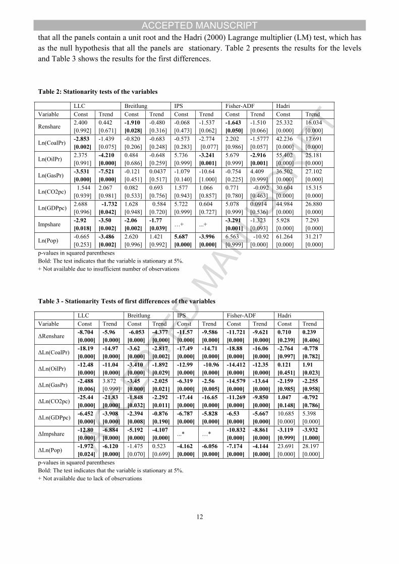
that all the panels contain a unit root and the Hadri (2000) Lagrange multiplier (LM) test, which has as the null hypothesis that all the panels are stationary. Table 2 presents the results for the levels and Table 3 shows the results for the first differences.
p-values in squared parenthesesBold: The test indicates that the variable is stationary at 5%.+ Not available due to insufficient number of observations
Table 3 - Stationarity Tests of first differences of the variables
p-values in squared parenthesesBold: The test indicates that the variable is stationary at 5%.+ Not available due to lack of observations
ACCEPTED MANUSCRIPT
13
Regarding the variables in levels, there is some doubt about the existence of a unit root for the dependent variable and the logs of the prices of oil, coal and gas. In these cases, even if at 5% significance level most of the tests point to the existence of a unit root, at 10% the results are mixed. For the logs of CO2, GDP per capita and of Population growth, the tests point overwhelming to non-stationarity while the Imports as share of consumption is considered to not have a unit root, except in the Hadri test (which has a null hypothesis that the variable is stationary for all countries).
However, looking to the same tests in first differences the overwhelming evidence is that the first differences are stationary, so the variables used in the model are a mixture of I(1) and I(0) which is a requirement to be able to estimate a panel ARDL.
Cointegration
Although cointegration of the variables is not strictly required, if it exists, the panel ARDL model has an error correction model interpretation and there is a stronger evidence that the long-run estimates are common across all countries, pointing to the PMG estimator.
We tested the data with the Pedroni (1999, 2004) and Westerlund (2005) tests, but we just included one fossil fuel price at a time, not only because there is a high level of correlation between oil and coal price, but also because as these variables do not present cross-country variation they may act as a sort of time-effect. Both tests have as null hypothesis no cointegration and allow panel-specific cointegrating vectors and that the AR coefficient in the auxiliary regression to vary over panels.
[0.000]p-values in squared parenthesesBold: The test indicates cointegration at 5%.
The results shown in Table 4 evidence that any combination of the variables with one fossil fuel price are cointegrated, giving support to estimate the model as an ARDL and interpret the coefficients of the variables in levels as the long-run impact on the dependent variable.
Results and discussion
Table 5 shows the long-run coefficients of the determinants of the adoption of renewable sources by the SSA countries considered. We opted to not transcribe the short run, as we use the PMG estimator that forces homogeneity in the long-run estimators but not on the short-run ones.
ACCEPTED MANUSCRIPT
14
Therefore, the short-run ones can vary from country to country and the mean group does not provide a good accuracy on the differences between countries.5
Furthermore, to ensure that the PMG estimator is adequate we used the Hausman test to test it against the Mean Group (MG) estimator (which allows heterogeneity in the short and long run estimators) which we know is consistent. The Hausman test did not reject the null in models (2) to (6), providing evidence that the PMG is consistent, and as it is more efficient, it provides more precise results.
Also, as can be seen in the appendix, the prices of coal and oil are highly correlated, which might lead to multicollinearity problems, and in fact it seems that these problems are present. First, when we omit one of the variables, the signs and significance of the effects of prices change (while the estimated coefficients of the remaining variables do not present such changes). Also, when we include all the prices, the Hausman test rejects the consistency of the PMG because in that model specification the long run effects vary substantially from country to country, which does not happen when we omit the Price of Coal or the Price of Oil (in all the other cases the Hausman test does not reject the null that the PMG estimators are consistent). This variation from country to country might be due to the imprecision because of the multicollinearity, which make us disregard the results of model 1 in Table 5.
N 408 408 408 408 408 408t statistics in parentheses* p < 0.10, ** p < 0.05, *** p < 0.01
5 The estimated model was an ARDL(1,1,…,1) model. The long run coefficients did not change much if we considered different lag lengths.
ACCEPTED MANUSCRIPT
15
Before analysing the variable coefficients we should mention that the estimated coefficient for the error correction mechanism (EC.coef) is in all cases significant, varying between -0.299 and -0.399 which means that on average the correction of shocks and deviations from the long-run path is done at considerable pace (considering that we are dealing with renewable production and, in many cases, the deployment of supply infrastructures) with half-life’s between 2,5 years and 3,3 years.
Looking for the different determinants first we can realise that the effect of the fossil fuels on the adoption of renewables is negative in the case of the Coal and, although not robust across regressions, the Oil and the Gas. This mixed effect of prices is not new in the literature: for instance, Marques et al. (2010) found a negative relation between coal prices and the use of renewables for non EU-members. This effect may have two different causes: first, as found by Chang et al. (2009), there is a threshold of the impact of an increased price of fossil fuels on renewables adoption as only countries with an high economic growth deal better with high energy prices, because it is easier to support the high costs connected with renewable technologies. In the current context, as we are studying SSA countries, which are mostly Low Income Countries the increase price on fossil fuels may divert resources from the building renewable energy infrastructures and so decrease the share of renewable generation on the overall mix. Second, this negative impact may be due to the lack of environmental restrictions, as fossil alternatives are better substitutes of each other, rather than renewable sources (see Van Ruijven and Van Vuuen, 2009).
Considering that we can proxy the environmental concerns through the emissions of CO2 per capita and the ratification of Kyoto protocol, we found for both variables a negative effect which is in contrast to the results found by Aguirre and Ibikunkle (2014), but for CO2 emissions in accordance with Marques et al. (2010). However, none of these two studies included any African country, so the environmental concerns due to an increase of CO2 or the awareness of the ratification of the Kyoto protocol were of no consequence to the adoption of renewable sources in the SSA countries. Furthermore, the ratification of Kyoto might even have the contrary effect, as it put less pressure in less developed countries as it might have been seen as signal that, at the moment, the SSA countries should not care much about CO2 emissions on the account of their development level.
Concerning the GDP per capita its signal is positive and robust across regressions, which is expected and consistent with previous studies for other regions as a country can invest more in renewable sources.
As for demand factors, population growth has a negative effect as energy use as a positive effect. This reflects two different realities, as population growth there is an increase of extensive demand for electricity, and as countries are pushed to supply more people, they resort to faster or cheaper ways to tap the increased demand and resort to fossil fuels. On the contrary, an increase in demand due to increased intensity (energy use) is also a signal of development and this lead SSA countries to plan the supply of these growth through cleaner sources. Finally concerning imports (which can be seen as the counterpart of energy security), an increase of imports leads to less dependence of renewables. In these cases, countries worried with energy security probably resort to fossil fuels rather than renewables for cost considerations. To the best of our knowledge, this study the first one to address this specific topic using this methodology, making inaccurate to provide a precise comparison with other studies. Nevertheless, the results are partially comparable to those of Salim e Rafiq (2012), Troster et al (2018), Iyke (2015) or Akinlo (2008).
ACCEPTED MANUSCRIPT
16
5. CONCLUSION
This research work aimed to identify the determinants of RE growth in SSA. This region has a great potential for developing RE such as wind, biomass, solar and hydropower, dispersed in all parts, which makes it an attractive place for RE investors. However, these potentials have not been fully employed, even though many of them are plentifully available, and have good economic potential with only hydropower at the moment having a substantial share in the regional energy mix.
From the study we found that the adoption of renewable sources is only undertaken if the country is getting more developed, being it measured by GDP per capita or energy use. All other variables, price of fossil fuels, imports, population growth, CO2 emissions have a negative effect. In some cases, these results contrast with what was found for richer economies, which is an indicator that the SSA countries, due to their level of income, try to overcome their challenges through cheaper or faster technologies and, therefore, they resort to fossil fuels. Furthermore, it seems that there is little or no concern about environmental problems, and that even the ratification of the Kyoto Protocol did little to promote the share renewables sources or even contributed to decrease it, as once the international community was happy to have it ratified, these countries pursued their own development agenda.
Taking it consideration the results obtained, it can be said that the main reasons that promote the use of renewable sources in SSA are economic, therefore in order to increase its usage in these countries other than waiting for growth and development would be to help these countries through aid programs that allow cheaper access to renewable sources and technical expertise in order to set up these facilitates at a faster pace. A second set of policies would be to encourage these countries to implement more serious environmental regulation and increase the environmental awareness of their economic agents. Together, these two mechanisms would make the use of renewables cheaper than the use of fossil fuels, and encourage the agents to shift from one to other.
One main limitation on the development of this study was the unavailability of data for most of the SSA countries, resulting in the use of only 17 countries for the analysis in the study. Nevertheless, it provides original results and offers possibilities for future work. These can include extending the number of countries used in the study based on data availability; analysing the impact of government policies on RE growth or investigating for the determinants of the growth of non-hydro RE.
ACCEPTED MANUSCRIPT
17
REFERENCES
Abas , N., Kalair , A., Khan , N. (2015). Review of fossil fuels and future energy technologies. Futures, 69, 31–49
Ackah, I., Kizys, R. (2015). Green growth in oil producing African countries: A panel data analysis of renewable energy demand. Renewable and Sustainable Energy Reviews, 50, 1157–1166.
Adams, S., Kwame, E., Klobodu, M., Evans, E., Opoku, O. (2016). Energy consumption , political regime and economic growth in sub- Saharan Africa. Energy Policy, 96, 36-44.
Aguirre, M., Ibikunle, G. (2014). Determinants of RE growth: A global sample analysis. Energy Policy, 69, 374-384.
Akinlo, A.E:, 2008, Energy consumption and economic growth: Evidence from 11 Sub-Sahara African countries, Energy Economics, 30, 2391–2400
Aliyu, A. K., Modu, B., Tan, C. W. (2018). A review of renewable energy development in Africa: A focus in South Africa, Egypt and Nigeria. Renewable and Sustainable Energy Reviews, 81, 2502-2518.
Anderson, T.W. and Hsiao, C., (1981). Estimation of dynamic models with error components. Journal of the American statistical Association, 76(375), pp.598-606.
Anderson, T.W. and Hsiao, C., (1982). Formulation and estimation of dynamic models using panel data. Journal of econometrics, 18(1), pp.47-82.
Apergis, N., Payne , J. E. (2010). RE consumption and economic growth: Evidence from a panel of OECD countries. Energy Policy, 38(1), 656-660.
Arellano, M. and Bover, O., (1995). Another look at the instrumental variable estimation of error-components models. Journal of econometrics, 68(1), pp.29-51.
Arellano, M., (1989). A note on the Anderson-Hsiao estimator for panel data. Economics Letters, 31(4), pp.337-341.
Augutis, J., Martišauskas, L., Krikštolaitis, R., Augutienơ, E. (2014). Impact of the Renewable Energy Sources on the Energy Security. Energy Procedia 61, 945 – 948.
Bird, L., Bolinger, M., Gagliano, T., Wiser, R., Brown, M., Parsons, B. (2005). Policies and market factors driving wind power development in the United States. Energy Policy, 33(11), 1397-1407.
Bazilian, M., Nussbaumer, P., Rogner, H.-H., Brew-hammond, A., Foster, V., Pachauri, S., . . . Kammen, D. M. (2012). Energy access scenarios to 2030 for the power sector in sub-Saharan Africa. Utilities Policy, 20(1), 1-16.
Breitung, J. and Das, S., (2005). Panel unit root tests under cross‐sectional dependence. Statistica Neerlandica, 59(4), pp.414-433.
Breitung, J., (2001). The local power of some unit root tests for panel data. In Nonstationary panels, panel cointegration, and dynamic panels (pp. 161-177). Emerald Group Publishing Limited.
Choi, I. (2001). Unit root tests for panel data. Journal of International Money and Finance 20: 249-272.
Carley, S. (2009). State RE electricity policies: An empirical evaluation of effectiveness. Energy Policy, 37, 3071-3081.
ACCEPTED MANUSCRIPT
18
Chang, T.-H., Huang, C.-M., Lee, M.-C. (2009). Threshold effect of the economic growth rate on the renewable energy development from a change in energy price: Evidence from OECD countries. Energy Policy, 37(12), 5796-5802.
Chassot, S., Hampl, N., Wüstenhagen, R. (2014). When energy policy meets free-market capitalists: The moderating influence of worldviews on risk perception and RE investment decisions. Energy Research and Social Science, 3, 143–151.
Chien, T., Hu, J.-l. (2008). RE: An efficient mechanism to improve GDP. Energy Policy, 36, 3045-3052.
Eberhard, A., Rosnes, O., Shkaratan, M., Vennemo, H. (2011). Africa's power infrastructure. investment, integration, efficiency. The International Bank for Reconstruction and Development / The World Bank, Washington.
Escribano Francés, G., Marín-Quemada , J. M., San Martín González, E. (2013). RES and risk: Renewable energy's contribution to energy security. A portfolio-based approach. Renewable and Sustainable Energy Reviews, 26, 549–559.
Foster, E., Contestabile, M., Blazquez, J., Manzano, B., Workman, M., Sha, N. (2017). The unstudied barriers to widespread renewable energy deployment: Fossil fuel price responses. Energy Policy, 103, 258-264.
Gan, Ã., Eskeland, G., Kolshus, H. (2007). Green electricity market development: Lessons from Europe and the US. Energy Policy, 35, 144-155
Hadri, K. (2000). Testing for stationarity in heterogeneous panel data. Econometrics Journal 3: 148-161.
Harris, R. D. F., and E. Tzavalis. (1999). Inference for unit roots in dynamic panels where the time dimension is fixed. Journal of Econometrics 91: 201-226.
Im, K. S., M. H. Pesaran, and Y. Shin. (2003). Testing for unit roots in heterogeneous panels. Journal of Econometrics 115: 53-74.
IEA. (2014). Africa Energy Outlook. International Energy Agency, Paris.IEA. (2015). World Energy Outlook 2015. International Energy Agency, Paris.IPCC. (2014). Climate Change 2014: Synthesis Report. Contribution of Working Groups I, II and
III to the Fifth Assessment Report of the Intergovernmental Panel on Climate Change [Core Writing Team, Pachauri, R.K., Meyer, L.A. (eds.)]. IPCC, Geneva, Switzerland, p. 151.
IRENA. (2018). Renewable Power Generation Costs in 2017. International Renewable Energy Agency, Available at http://www.irena.org/publications/2018/Jan/Renewable-power-generation-costs-in-2017.
Iyke, . (2015),Electricity consumption and economic growth in Nigeria: A revisit of the energy-growth debate, Energy Economics, 51 166–176
Abu Dhabi.Kilinc-ata, N. (2016). The evaluation of renewable energy policies across EU countries and US states: An econometric approach. Energy for Sustainable Development, 31, 83-90.
Maria, L., Bernauer, T. (2014). Explaining government choices for promoting renewable energy. Energy Policy, 68, 15-27.
Kumar, R., & Agarwala, A. (2016). Renewable energy technology diffusion model for technoeconomics feasibility. Renewable and Sustainable Energy Reviews, 54, 1515–1524.
Levin, A., C.-F. Lin, and C.-S. J. Chu. (2002). Unit root tests in panel data: Asymptotic and finite-sample properties. Journal of Econometrics 108: 1-24
Marques, A. C., Fuinhas, J. A. (2012). Are public policies towards RE successful? Evidence from European countries. Renewable Energy, 44, 109-118.
Marques, C., Fuinhas, A., Manso, J. (2010). Motivations driving RE in European countries: A panel data approach. Energy Policy, 38, 6877-6885.
Menegaki, A. N. (2011). Growth and renewable energy in Europe: A random effect model with evidence for neutrality hypothesis. Energy Economics, 33(2), 257-263.
Menz, F., Vachon, S., (2006). The effectiveness of different policy regimes for promoting wind power: experiences from the States. Energy Policy 34, 1786–1796.
Mukasa, A. D., Mutambatsere, E., Arvanitis, Y., Triki, T. (2015). Energy Research and Social Science Wind energy in sub-Saharan Africa: Financial and political causes for the sector’s under-development. Energy Research and Social Science, 5, 90-104.Nesta, L., Vona, F., Nicolli, F. (2014). Environmental policies, competition and innovation in renewable energy. Journal of Environmental Economics and Management, 67(3), 396-411.
Ohler, A., Fetters, I. (2014). The causal relationship between renewable electricity generation and GDP growth: A study of energy sources. Energy Economics, 43, 125–139.
Omri, A., Khuong, D. (2014). On the determinants of renewable energy consumption: International evidence. Energy, 72, 554-560.
Pablo, R. (2005). The implications of the Kyoto project mechanisms for the deployment of renewable electricity in Europe. Energy Policy, 33, 2010-2022
Pedroni, P. (1999). Critical values for cointegration tests in heterogeneous panels with multiple regressors. Oxford Bulletin of Economics and Statistics 61: 653-670.
Pedroni, P. (2004). Panel cointegration: Asymptotic and finite sample properties of pooled time series tests with an application to the PPP hypothesis. Econometric Theory 20: 597-625
Pesaran, M. H., Y. Shin, and R. P. Smith (1999). Pooled mean group estimation of dynamic heterogeneous panels. Journal of the American Statistical Association 94: 621–634.
Pesaran, M. H., and R. P. Smith. 1995. Estimating long-run relationships from dynamic heterogeneous panels. Journal of Econometrics 68: 79–113.
Pfeiffer, B., Mulder, P. (2013). Explaining the diffusion of RE technology in developing countries. Energy Economics, 40, 285-296.
Polzin, F., Migendt, M., Taube, F. A., von Flotow, P. (2015). Public policy influence on renewable energy investments - A panel data study across OECD countries. Energy Policy, 80, 98-111.
Popescu, G. H., Mieila, M., Nica, E., Andrei, J. V. (2018). The emergence of the effects and determinants of the energy paradigm changes on European Union economy. Renewable and Sustainable Energy Reviews, 81, 768-774.
Popp, D., Hascic, I., & Medhi, N. (2011). Technology and the diffusion of renewable energy. Energy Economics, 33(4), 648-662.
Prasad, G. (2011). Improving access to energy in sub-Saharan Africa. Current Opinion in Environmental Sustainability, 3(4), 248-253.
Rafiq, S., Bloch, H. Salim, R.Determinants of Renewable Energy Adoption in China and India: A Comparative Analysis, Applied Economics 46, 22, 2700-2710
Reboredo, J. C. (2015). Is there dependence and systemic risk between oil and renewable energy stock prices? Energy Economics, 48, 32-45.
ACCEPTED MANUSCRIPT
20
Rupf, G. V., Bahri, P. A., Boer, K., Mchenry, M. P. (2016). Broadening the potential of biogas in Sub-Saharan Africa: An assessment of feasible technologies and feedstocks. Renewable and Sustainable Energy Reviews, 61, 556-571.
Rüstemoglu , H., Andrés , A. R. (2016). Determinants of CO2 emissions in Brazil and Russia between 1992 and 2011: A decomposition analysis. Environmental Science and Policy, 58, 95-106.
Sadorsky, P. (2009a). RE consumption, CO2 emissions and oil prices in the G7 countries. Energy Economics, 31, 456-462.
Sadorsky, P. (2009b). RE consumption and income in emerging economies. Energy Policy, 37, 4021-4028.
Salim, R., Rafiq, S. , 2012, Why do some emerging economies proactively accelerate accelerate the adoption of renewable energy? , Energy Economics 34 1051–1057
Siddiqui, A. S., Tanaka, M., Chen, Y. (2016). Are targets for renewable portfolio standards too low? The impact of market structure on energy policy. European Journal of Operational Research, 250, 328-341.
Stadelmann, M., Castro, P. (2014). Climate policy innovation in the South – Domestic and international determinants of RE policies in developing and emerging countries. Global Environmental Change, 29, 413-423.
Suberu, M. Y., Wazir, M., Bashir, N., Asiah, N., Safawi, A. (2013). Power sector RE integration for expanding access to electricity in sub-Saharan Africa. Renewable and Sustainable Energy Reviews, 25, 630-642.
Troster, V., Shahbaz, M. ,Uddin, G., 2028. Renewable energy, oil prices, and economic activity: A Granger-causality in quantiles analysis, Energy Economics 70 440–452
Valdés Lucas, J. N., Escribano Francés, G., San Martín González, E. (2016). Energy security and renewable energy deployment in the EU: Liaisons Dangereuses or Virtuous Circle? Renewable and Sustainable Energy Reviews 62, 1032–1046.
Van Ruijven, B., Van Vuuren, D. P. (2009). Oil and natural gas prices and greenhouse gas emission mitigation. Energy Policy, 37(11), 4797-4808.
WB. (2013). Low-Carbon Development Opportunities for Nigeria. International Bank for Reconstruction and Development / The World Bank, Washington.
WB. (2016). World Development Indicators. International Bank for Reconstruction and Development / The World Bank, Washington.
Wiser, R., Namovicz, C., Gielecki, M., Smith, R. (2007). Renewables Portfolio Standards: A Factual Introduction to Experience from the United States. Ernest Orland Lawrence Berkeley National Laboratory.
.Westerlund, J. (2005). New simple tests for panel cointegration. Econometric Reviews 24: 297-316.