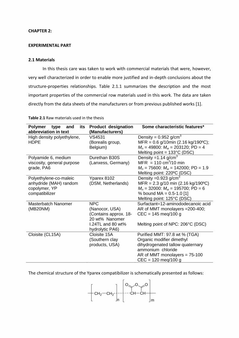
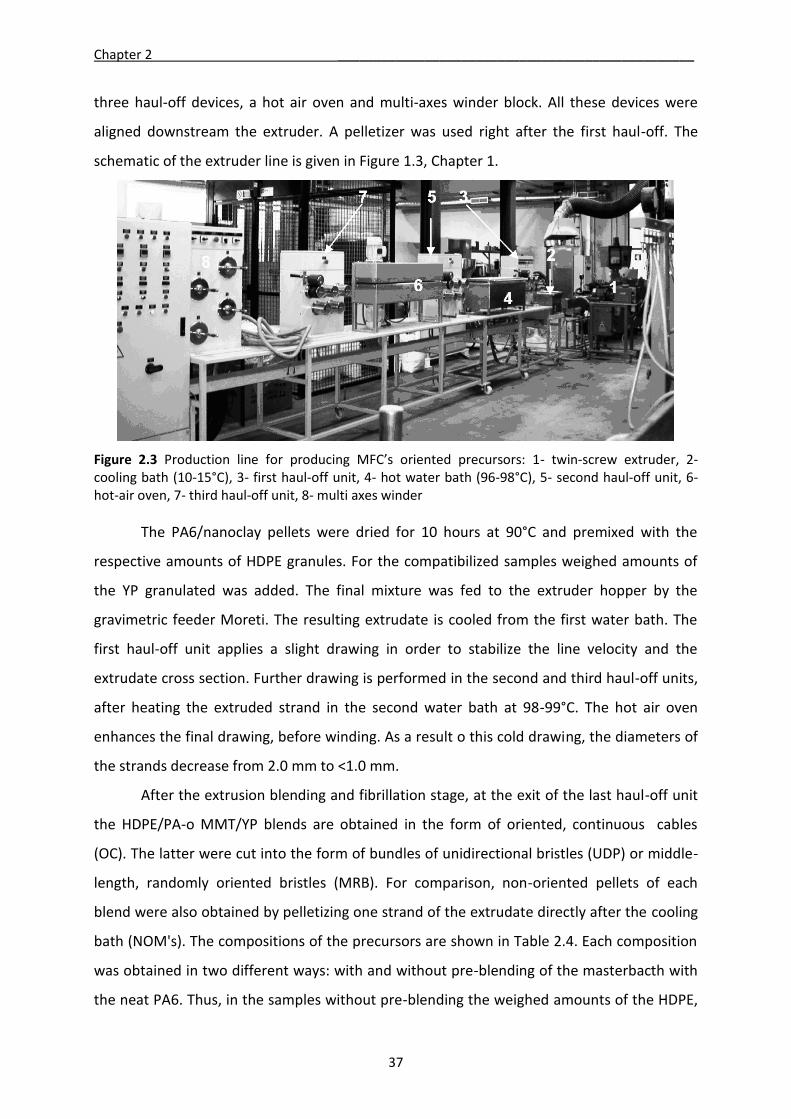
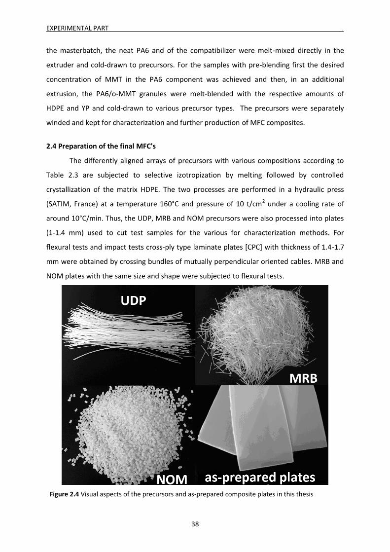
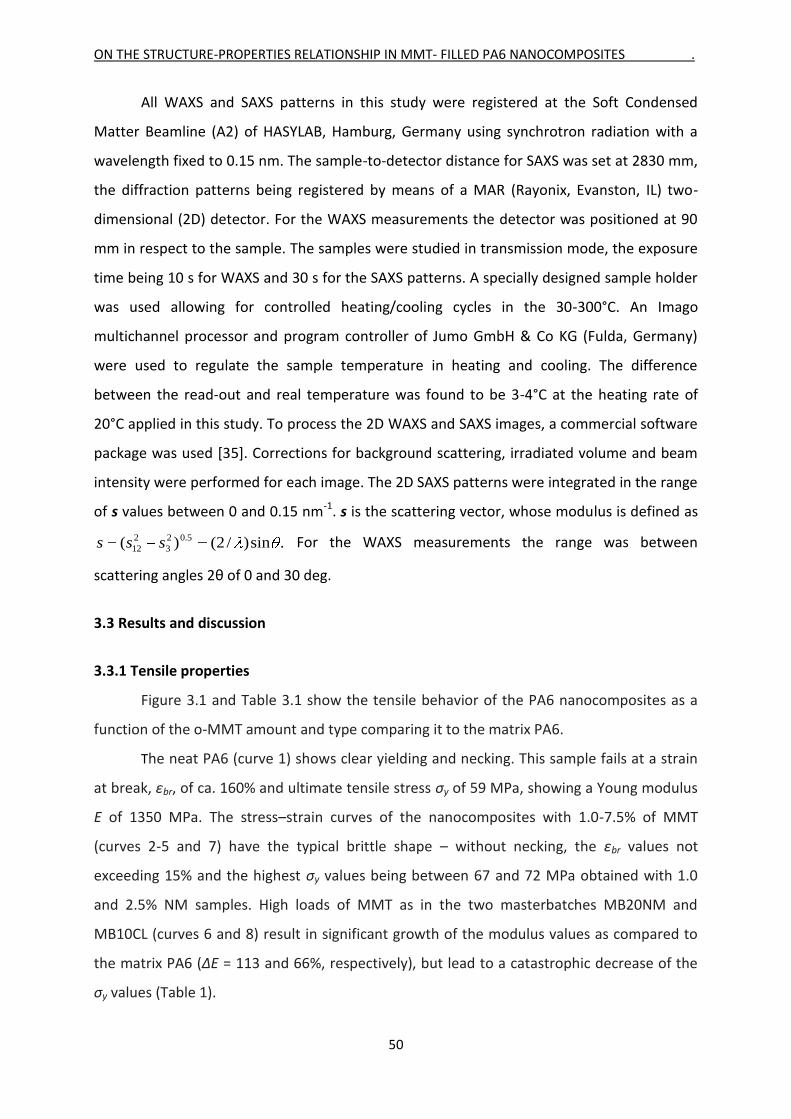
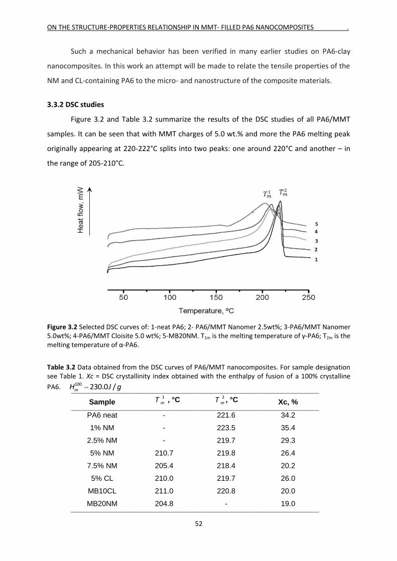
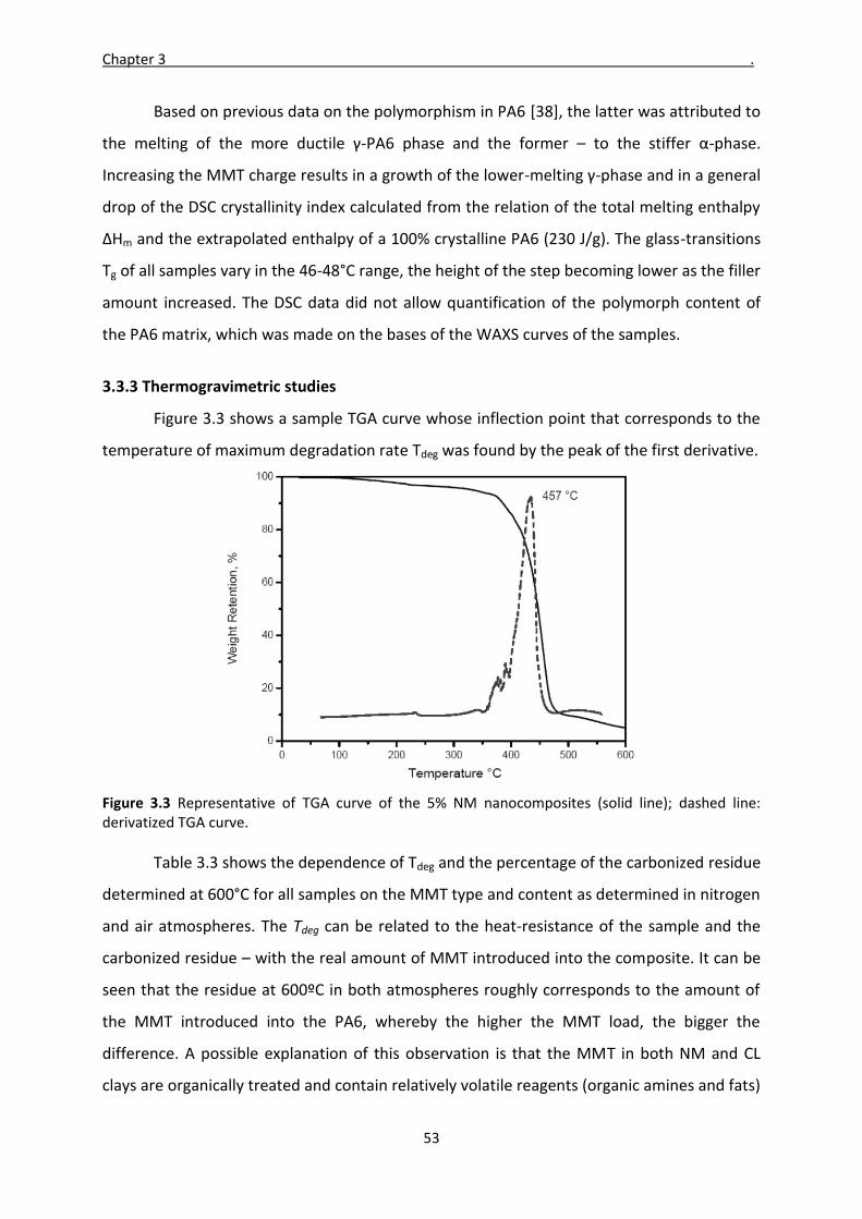
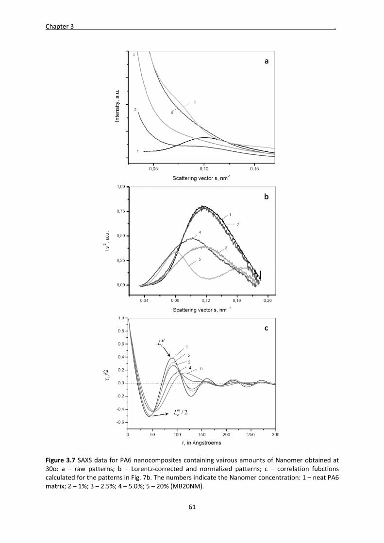
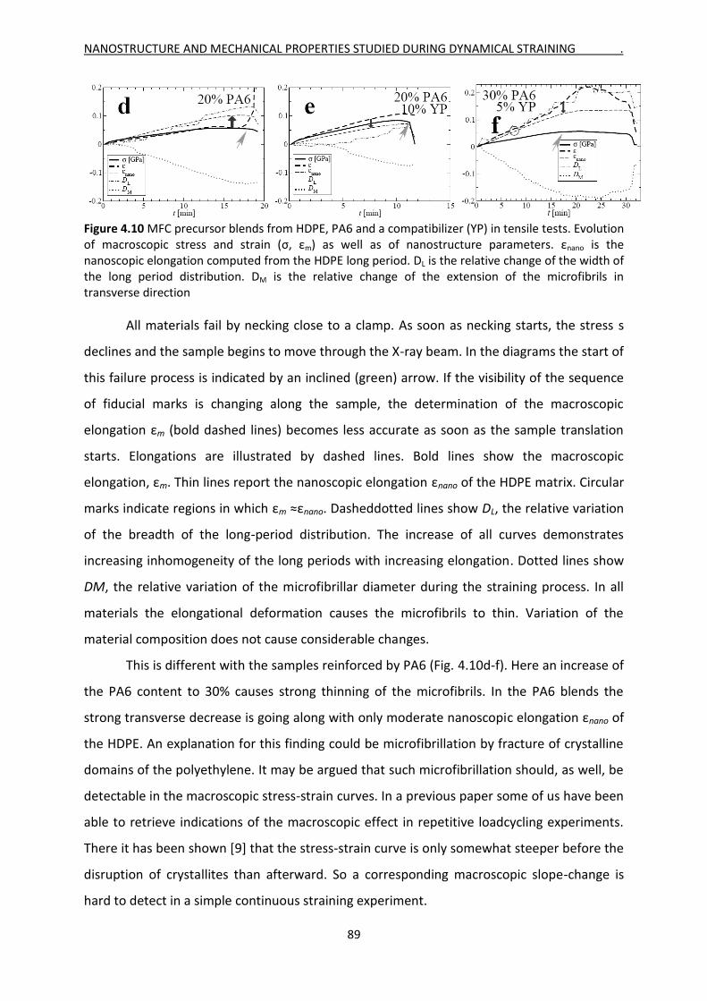
Development and Investigation of New Hybrid Composite ... · diferentes alinhamentos e geometrias...

M

lade

n Fe

odor

ov M

otov

ilin

Março de 2011UMin

ho |

201

1De

velo

pmen

t and

Inve

stig

atio

n of

New

Hyb

rid

Com

posi

te M

ater

ials

Bas

edon

Orie

nted

Ble

nds

of T

herm

opla

stic

Pol

ymer

s an

d N

anos

ized

Inor

gani

c Fi

llers

Universidade do MinhoEscola de Engenharia

Mladen Feodorov Motovilin

Development and Investigation ofNew Hybrid Composite Materials Based onOriented Blends of Thermoplastic Polymersand Nanosized Inorganic Fillers

Março de 2011

Tese de DoutoramentoCiência e Engenharia de Polímeros e Compósitos

Trabalho efectuado sob a orientação doProfessor Doutor Zlatán Zlatev Dénchev

Mladen Feodorov Motovilin

Development and Investigation ofNew Hybrid Composite Materials Based onOriented Blends of Thermoplastic Polymersand Nanosized Inorganic Fillers

Universidade do MinhoEscola de Engenharia

To Irina, Nadia, Victor and my family

ACKNOLEDGMENTS

This research scientific work was performed in the University of Minho, Guimarães

and Braga, Portugal, in the Department of Polymer Engineering, Institute for Polymers

and Composites, which is part of the i3N Associated Laboratory. The X‐ray synchrotron

measurements were performed at the German Synchrotron Facility (DESY) ‐ HASYLAB,

Hamburg, Germany. It could not be done without the inspiration, help, discussion and

influence from the following people:

‐ Prof. Dr. Zlatan Denchev‐ supervisor the whole thesis, I am grateful to all his

support, practical, technical and theoretical help in any aspect of the work.

‐ Prof. Dr. Norbert Stribeck for his technical and scientific support in SAXS

measurements, his performance of the SAXS straining of the polymer blends and

developing the methods for analysis and the excellent results.

‐ Dr. Nadya Dencheva for helping me for the X‐ray analysis and processing of data,

practical and theorical aspects of the the thesis.

‐ Dr. Stanislav Ferdov for X‐ray measurements, excellent professional attitude, help

and friendship.

‐ Technical staff of the Department of polymer Engineering, namely: João Paulo

Peixoto for the extruder part and for his big friendship, Eng. Mauricio Malheiro for

the thermal analysis, microscopy, FT‐IR analysis and good advices for the practical

aspects of the experiments, Serafim Sampaio for the compression molding press

and repairment and injection modling, Francisco Mateus and Manuel Escourido

for the compression molding and mechanical testing.

‐ PIEP organization for giving me the opportunity to perform the impact tests.

‐ Technical staff of SEM laboratory in UMinho, Braga, namely Elsa Ribeiro for all the

good help and measurements.

‐ Dr. Rui Fernandes for the TEM images and sample preparation.

I gratefully acknowledge the financial support of Fundação para a Ciência e

Tecnologia, Portugal; with my grant number SFRH/BD/30121/2006, also the financial

support of the Hamburg Synchrotron laboratory (HASYLAB) at the German

Synchrotron Facility (DESY) under project DESY‐D‐II‐07011EC. Special thanks to Dr.

v

Sérgio Funari, scientist at the A2 Beamline in DESY for scientific, practical and

technical help and support through all the missions there.

I wish to thank to all the people working and accepting me in the Polymer

Department, namely: Dr.Mikio Yamanoi for theoretical and practical help and big

friendship, Prof. Dr. Satyabratta Ghosh for his advices, Luis Ferras, Dr. Weidong Zhang

for theoretical advices and Origin help, Prof. Rui Novais, Filomena Costa, Eng. Paulo

Teixeira, Eng. Pedro Marques, Dr. Joana Barbas, Eng. Renato Reis, Eng. Liliana Rosa,

Isabel Moura and all the rest of the people here in the department.

Special thanks to eng. Franziska Riegel, Ana Matveeva and eng. Mauro Rabuski for

moral and friendly support for finishing the thesis.

This work will also not be done without the support and friendship from my

compatriots: Dr. Lyudmil Todorov, Eng. Milena Tomanova, Dr. Angel Yanev, Dr. Diana

Krasteva, Eng. Nikolay Marinov, Eng. Petya Peneva. All of them helped and

encouraged me a lot in the moments of my stay in Portugal.

Finally I wish to thank to especially Irina Georgieva, Viktor Stankov, Simeon

Ribagin, without their friendship and support this will never be realized, written and

published. I wish to thank a lot for my sister Nadia for moral support and spiritual help

during the years abroad and my family for support and belief in me always.

Mladen Motovilin,

Guimarães, March 2011

vi

RESUMO

Nano‐compósitos à base de poliamida‐6 (PA6) e nano‐argilas de montmorillonite

(MMT), foram produzidos utilizando‐se duas marcas comerciais: (i) masterbatch Nanomer

I.24TL com 20% em massa de MMT em PA6 hidrolítica; (ii) Cloisite 15A em pó,

organicamente tratada. O masterbatch Nanomer foi diluído numa extrusora duplo fuso

para 1,0; 2,5; 4,0; 5,0 e 7,5 % em massa. Um masterbatch de 10% foi preparado

laboratorialmente através da extrusão de PA6 com Cloisite 15A, e posteriormente diluído

para 4 e 5% de percentagem massiças da componente MMT. Amostras (placas)

preparadas por moldação por compressão de todos os híbridos, passaram por testes

mecânicos, térmicos e de análise estrutural. Os testes de tracção revelaram que,

aumentando a percentagem de MMT, o módulo de elasticidade aumenta, enquanto a

deformação à ruptura diminui. As análises térmicas foram utilizadas com o propósito de

se testar a forma como a nano‐argila afecta a estabilidade térmica, assim como a

concentração das formas polimórficas da matriz PA6. Ensaios de difracção de raios X em

ângulos altos e baixos (WAXS e SAXS) provaram o tipo da distribuição de MMT, assim

como a sua influência sobre a nanoestrutura da matriz PA6. As técnicas de FT‐IR com

microscopia óptica e de microscopia electrónica (SEM e TEM) complementaram os

estudos estruturais dos híbridos PA6‐MMT.

Os híbridos de PA6‐MMT assim caracterizados foram misturados numa extrusora

de duplo fuso com polietileno de alta densidade (HDPE), com e sem compatibilizador

Yparex (YP), para produzir misturas precursoras orientadas com as composições

HDPE/PA6‐MMT/YP = 80/20/0 e 77.5/20/2.5. Esses precursores orientados foram

transformados em vários tipos de compósitos microfibrilares (MFC), através de fusão

selectiva do constituinte HDPE, por moldação por compressão a 160°C. Compósitos com

diferentes alinhamentos e geometrias dos reforços de PA6 foram produzidos desde cada

composição HDPE/PA6‐MMT/YP, nomeadamente: lâminas unidireccionais (UDP);

laminados com lâminas de orientação cruzada (CPC); placas de filamentos com

comprimento médio e orientação aleatória (MRB). Compósitos não orientados (NOM) de

misturas de HDPE/PA6‐MMT/YP foram também produzidas por compressão ou moldação

por injecção. Todos os materiais UDP, MRB e NOM, foram testados à tracção; os CPCs

passaram nos testes de flexão e impacto. Amostras de UDP apresentaram os maiores

vii

módulos de Young (especialmente aqueles com maiores percentagens de MMT), boa

resistência aos ensaios de tracção, de flexão e impacto, apresentando melhores

resultados comparativamente aos de matriz com HDPE, e em muitos casos melhor que o

respectivo MFCs sem o reforço MMT.

Os dados provenientes das medições WAXS e das experiências simultâneas de

SAXS/extensão, discutidas em conjunto com as amostras morfológicas através do SEM,

mostraram que a transcristalização do HDPE sobre as fibras da PA6 adicionalmente

reforçado por MMT, têm uma influência importante no desempenho mecânico dos

compostos híbridos UDP.

viii

ABSTRACT

Nanocomposites based on polyamide‐6 (PA6) and montmorillonite (MMT)

nanoclays were produced using two commercial brands: (i) a masterbatch of Nanomer

I24TL with 20 wt % MMT in hydrolytic PA6 and (ii) organically treated powder‐like Cloisite

15A. The Nanomer masterbatch was diluted in twin‐screw extruder to 1, 2.5, 4, 5 and 7.5

wt%. A 10% masterbatch was prepared locally by extrusion of PA6 with Cloisite 15 A and

then diluted to 4 and 5 wt% MMT content. Compression molded plates prepared from all

hybrids passed through mechanical, thermal and structural analyses. The tensile tests

revealed that with increasing the MMT content the Young modulus increases, while the

elongation at break decreases. Thermal analyses were used to test how the nanoclay

affects the thermal stability and the polymorph concentration of the PA6 matrix.

Synchrotron wide and small‐angle X‐ray scattering (WAXS, SAXS) probed the MMT

distribution and also its influence on the nanostcruture of the matrix. The structural

characterization of the PA6‐MMT hybrids was complemented by FT‐IR microcopy and

electron microscopy methods (SEM and TEM).

The well‐characterized PA6‐MMT hybrids were blended in a twin‐screw extruder

with high‐density polyethylene (HDPE), with and without compatibilizer Yparex (YP), to

produce oriented precursor blends with compositions HDPE/PA6‐MMT/YP=80/20/0 and

77.5/20/2.5, the PA6 constituent comprising the above amounts and types of MMT.

These oriented precursors were transformed into various types of microfibrillar

composites (MFC) by selectively melting the HDPE constituent by compression molding at

160°C. Composites with different alignment and geometry of the PA6 reinforcements

were produced from each HDPE/PA6‐MMT/YP composition: unidirectional ply laminae

(UDP), cross‐ply laminates (CPC), and MFCs from middle‐length, randomly oriented

bristles (MRB). Composites from non‐oriented HDPE/PA6‐MMT/YP mixtures (NOM) were

also produced by compression‐ or injection molding. All UDP, MRB and NOM materials

were tensile tested; the CPC passed flexural and impact tests. The UDP samples

demonstrated the highest modulus, especially the ones with highest MMT content, good

tensile strength, flexural and impact properties, being better than those of the HDPE

matrix, and in many cases better than the respective MFCs without MMT reinforcement.

ix

The data from the WAXS measurements and from the simultaneous

SAXS/straining experiments, discussed in conjunction with sample morphology by SEM

showed that the transcrystallization of HDPE onto the PA6 fibrils additionally reinforced

by MMT, has an important role for the mechanical performance of the UDP hybrid

composites.

x

TABLE OF CONTENTS

Acknowledgements v Resumo vii Abstract ix Table of contents xi List of symbols and abbreviations xv CHAPTER 1 POLYAMIDE BASED NANO‐ AND MICROFIBRILLAR COMPOSITES: STATE OF THE ART 1

1.1 Introduction 1

1.2 Polymer‐clay nanocomposites 2

1.2.1 Polyamide/nanoclay composites 5

1.3 Microfibrillar composites‐literature survey 10

1.3.1 Preparation of MFCs 13

1.3.2 Mechanical characterizationof PE/PA microfibrillar composites 17

1.3.3 Morphology and structure investigations of MFCs 19

1.4 Research goal and structure of the thesis 23

1.5 References 26

CHAPTER 2 EXPERIMENTAL PART 34

2.1 Materials 34

2.2 Production of polyamide‐6/nanoclay masterbatches and nanocomposites 35

2.3 Production of HDPE/PA6‐oMMT/YP oriented precursors 36

2.4 Preparation of the final MFCs 38

2.5 Injection molding 39

2.6 Sample characterization 39

2.6.1 Thermal analysis 39

2.6.2 FT‐IR 40

2.6.3 Microscopy tests 40

xi

2.6.4 Mechanical tests 40

2.6.5 Synchrotron X‐ray scattering techniques 43

2.7 References 45

CHAPTER 3 ON THE STRUCTURE‐PROPERTIES RELATIONSHIP IN MONTMORILLONITE‐FILLED POLYAMIDE 6 NANOCOMPOSITES 45

3.1 Introduction 47

3.2 Experimental details 48

3.2.1 Raw materials 48

3.2.2 PA6/MMT compounding and test sample preparation 48

3.2.3 Sample analysis 49

3.3 Results and discussions 50

3.3.1 Tensile properties 50

3.3.2 DSC studies 52

3.3.3 Thermogravimetric studies 53

3.3.4 Structural analysis by WAXS 54

3.3.5 Structural studies by SAXS 60

3.3.6 FT‐IR microscopy 63

3.3.7 TEM 65

3.4 Conclusions 67

3.5 References 68

CHAPTER 4 NANOSTRUCTURE AND MECHANICAL PROPERTIES STUDIED DURING DYNAMICAL STRAINING OF MICROFIBRILLAR REINFROCED HDPE/PA BLENDS 71

4.1 Introduction 71

4.2 Methods 73

4.2.1 A correlation method to determine the macroscopic elongation from sample

photos 73

4.2.2 Automated 2D peak analysis in scattering patterns 76

4.3 Experimental details 79

4.3.1 Materials 79

xii

4.3.2 Straining environment 80

4.3.3 SAXS environment 81

4.3.4 Data evaluation 81

4.4 Results and discussion 81

4.4.1 HDPE/PA blends. Mechanisms explaining the recorded structure evolution

82

4.4.2 HDPE/PA6/nanoclay blends. Mechanisms explaining the recorded structure

evolution 83

4.4.3 Nanostructure evolution: Scattering patterns 84

4.4.4 Nanostructure evolution: Quantitative analysis 88

4.4.5 Measured mechanical properties 94

4.4.6 Nanostructure and mechanical properties 96

4.5 Conclusions 97

4.6 References 97

CHAPTER 5 MECHANICAL PROPERTIES OF THE READY MICROFIBRILLAR COMPOSITES 100

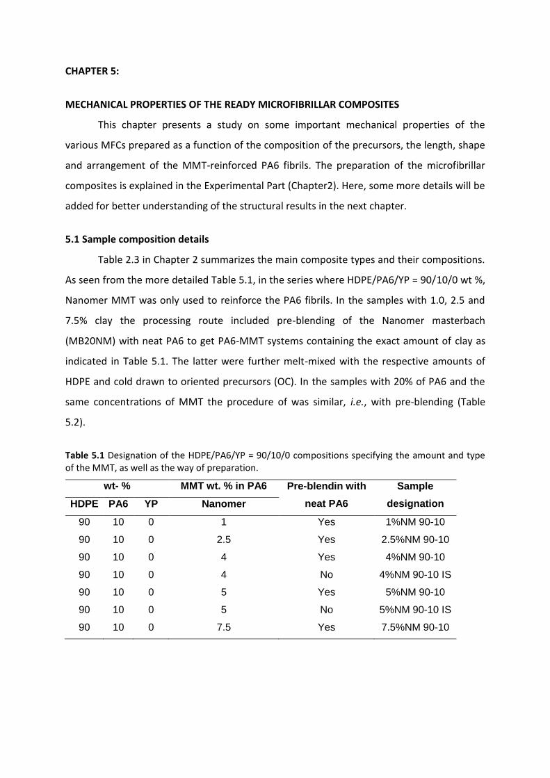
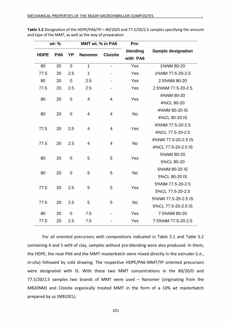
5.1 Sample composition details 101

5.2 Tensile properties of UDP composites 102

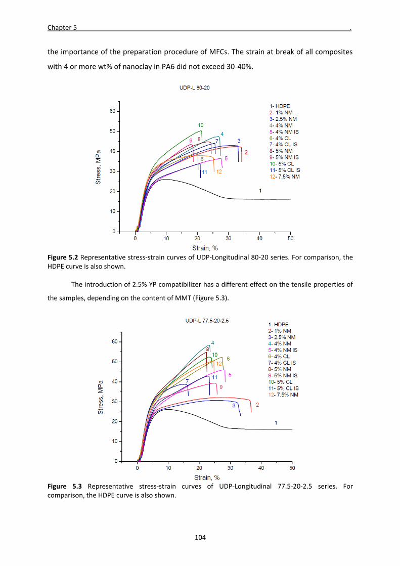
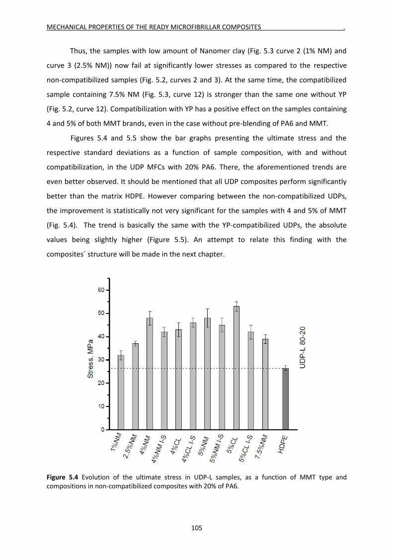
5.2.1 Stress‐strain curves 102

5.2.2 Longitudinal and transversal tensile behavior of UDPs 106

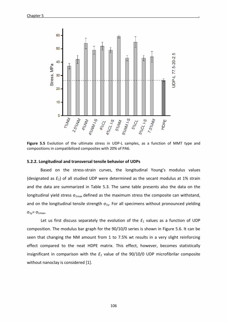
5.3 Tensile properties of MRB and NOM composites 112

5.3.1 MRB Composites 112

5.3.2 NOM composites 113

5.3.3 Tensile properties of UDP, MRB and NOM – a comparison 115

5.4 Flexural properties of CPC MFCs 117

5.5 Impact tests of selected CPC MFCs 120

5.6 References 123

CHAPTER 6 STRUCTURE DEVELOPMENT OF UDP MFC AND ITS RELATIONSHIP WITH THE MECHANICAL PROPERTIES 124

6.1 SEM imaging 124

xiii

6.2 2D WAXS anaysis 130

6.2.1 Isotropic WAXS fraction – fitting 132

6.2.2 Oriented WAXS fraction – fitting 138

6.2.3 Evolution of isotropic and oriented WAXS with temperature 143

6.3 Simultaneous SAXS/straining experiments with HDPE/PA6 UDP composites 146

6.4 References 160

CONCLUSIONS 162

RECOMMENDATIONS FOR FUTURE WORK AND RESEARCH 167

xiv

LIST OF SYMBOLS AND ABBREVIATIONS

Latin symbols

CR, MPa ‐ reduced flexural stiffness

E1, MPa ‐ tensile modulus in longitudinal direction

E2, MPa ‐ tensile modulus in transversal direction

E*, MPa ‐ complex modulus

Ef, MPa ‐ modulus of the fibers

LB, nm ‐ Bragg long spacings

lc, Å ‐ average thickness of the crystal lamellae

la, Å ‐ average thickness of the amorphous region

s, nm‐1, Å‐1 ‐ scattering vector

Tdeg, °C ‐ temperature of degradation

Tg, °C‐ glass transition temperature

Tm, °C ‐ melting temperature

Vf ‐ volume fraction

Greek symbols

α‐ alpha form of polyamide‐6

γ‐ gama form of polyamide‐6

ε, mm or % ‐ strain

εbr ‐ strain at break

εnano‐ nanoscopic elongation

λ (dimensionless) ‐ draw ratio

λ, Å ‐ X‐ray radiation wavelenght

σ, MPa ‐ tensile stress

σfmax ‐ strength of a fiber

σpmax ‐ strength of a matrix

ρ‐ density

xv

Abbreviations

AFM ‐ atomic force microscopy

AR ‐ aspect ratio

CDF ‐ cord distribution function

CEC ‐ cation exchange capacity

CF ‐ correlation function

CL ‐ Cloisite 15A

CM ‐ compression molding

CNT ‐ carbon nanotube

CPC – cross‐ply composite

DSC ‐ differential scanning calorimetry

DTMA ‐ dynamic thermo mechanical analysis

FT‐IR ‐ Fourier‐transform infrared spectroscopy

GF ‐ glass fiber/s

GPC ‐ gel permeation chromatography

HDPE ‐ high density polyethylene

iPP ‐ isotactic polypropylene

IF ‐ improvement factor

IM ‐ injection molding

IR ‐ infrared

LCP ‐ liquid crystalline polymer

LDPE ‐ low density polyethylene

LLDPE ‐ linear low density polyethylene

MA ‐ maleated

MAH ‐ maleic anhydride

MB20NM ‐ masterbatch with 20% nanoclay, Nanocor, USA

MB10CL ‐ masterbatch with 10% nanoclay Cloisite 15A

MFC/MFCs ‐ microfibrillar composite/s

MFR ‐ Melt Flow rate

MMT ‐ Montmorillonite

MRB ‐ middle random bristles

xvi

xvii

NM ‐ Nanomer

NMR ‐ nuclear magnetic resonance

NOM ‐ non‐oriented mixture

o‐MMT ‐ organically treated montmorillonite

OC ‐ oriented cable

PA6 ‐ polyamide‐6

PA66 ‐ polyamide‐66

PA12 ‐ polyamide‐ 12

PBT ‐ poly butylene terephtalate

PC ‐ polycarbonate

PD ‐ polydispercity ratio

PE ‐ polyethylene

PET ‐ polyethylene terephtalate

PLM ‐ polarized light microscopy

PP ‐ polypropylene

S, MPa ‐ shear strength (Tsai‐Hill)

SAXS ‐ Small‐angle X‐ray scattering

SEM ‐ scanning electron microscopy

TCL ‐ transcrystalline layer

TEM ‐ transmission electron microscopy

TG ‐ thermogravimetry, thermogravimetrical

TGA –thermogravimetrical analysis

UDP ‐ uni‐directional ply

UDP‐L ‐ longitudinal uni‐directional ply

UDP‐T ‐ transversal uni‐directional ply

WAXS ‐ Wide‐angle X‐ray scattering

WAXD ‐ Wide‐angle X‐ray diffraction

X, MPa ‐ tensile strength in the fiber direction (Tsai‐Hill)

XRD ‐ x‐ray diffraction

Y, MPa ‐ tensile strength in the transverse direction (Tsai‐Hill)

YP ‐ Yparex compatibilizer from DSM

CHAPTER 1:

POLYAMIDE BASED NANO- AND MICROFIBRILLAR COMPOSITES: STATE OF THE ART

1.1 Introduction

An acceptable composite material for use in engineering applications should satisfy

the following three basic requirements [1]: (i) to consist of at least two physically distinct and

mechanically separable materials, which, depending on their properties and amounts used,

are called matrix (medium) and reinforcing component; (ii) there must be a possibility for its

preparation by admixing of the above components (sometimes preceded or accompanied by

some special treatment so as to achieve optimum properties); and (iii) the final material is

expected to possess several properties being superior to that of the individual components,

i.e. some synergistic effect should be present. The realization of this synergism requires

strictly defined and reproducible distribution of the size and dispersity of the reinforcing

component within the matrix, as well as a good adhesion and certain compatibility of the

separate phases forming the composite [2]. In other words, the reason to produce

composites is to obtain properties that the matrix and reinforcing components cannot

achieve acting alone. It should be noted that these two basic components may be metallic,

ceramic or polymeric [1].

Manufacturing of composites in which at least one of both of the components are

polymeric have become one of the biggest branches of polymer industry the products of

which combine different properties. First polymer composites were developed several

decades ago. Considerable advances have been made since then in the use of these

materials and applications developed in the construction, automotive, spaceship, packaging

and other sectors. The material properties of the final component are the result of a design

process that considers many factors which are characterized by the anisotropic behavior of

the material and cover the micro-mechanical, elasticity, strength and stability properties.

These properties are influenced by manufacturing techniques, environmental exposure and

loading histories. Designing with composites is thus an interactive process between the

design of the constituent materials used, the design of the composite material and an

understanding of the manufacturing technique for the composite component.

Chapter 1_____________________ ___________

2

With respect to the size of the reinforcing component, polymer composites can be

divided into three basic groups: (i) macrocomposites, comprising reinforcements with

relatively large sizes (most frequently above 0.1mm) of glass, carbon or some special rigid

polymers; (ii) nanocomposites, where the reinforcements (typically inorganic) have at least

one of their dimensions in the nanometer length scale and (iii) molecular composites, where

the reinforcement is built up from single, rigid-rod macromolecules with diameters in the

angstrom range. Based on the shape of the reinforcing entities, one can distinguish fibers (or

one-dimensional), plate-like (two-dimensional) and powder-like (three-dimensional) fillers

[3].

Examples for conventional macrocomposites are the fiber-reinforced systems

consisting of an isotropic matrix made out of a polyolefin, polyamide, polyester, etc., that

embeds organic or inorganic fibers of various lengths and arrangement with diameters

typically larger than 1 μm. The fibers can be made of glass, carbon or Kevlar [4,5]. Nowadays

conventional polymer composites are important commercial materials with a wide range of

applications in many industries (e.g., aerospace, automotive etc) where highly resistant and

lightweight materials are of prime importance. In recent years, however, optimizing the

properties of these traditional polymer composites containing micrometer-scale reinforcing

entities has reached its limits [3]. The advent of the nanostructured polymer composites

opened a large window of opportunities to further improve the mechanical properties. Good

examples of nanocomposites are the carbon nanotube (CNT)-reinforced systems [6]. Clay-

reinforced polymer composites that belong to the systems reinforced by two-dimensional

nanofillers have significant importance in many industries and being the subject of numerous

scientific publications [7-10]. A short review of the novel trends in polymeric

nanocomposites was given recently by Mark [11].

With some approximation, liquid crystalline polymer (LCP) containing composites can

be considered the closest example of molecular composites. By virtue of their molecular

structure and conformation, the LCP reinforcements tend to form in situ, during processing,

very fine fibers having similar or better reinforcing efficiency as compared to that of

conventional inorganic fibers [12]. A substantial amount of work has also been performed in

the area of LCP-containing composites described in numerous publications [13-16]. Due to

the quite complex processing of LCP composites resulting in their high price, a substantial

breakthrough in the industrial application of these materials has not yet occurred.

POLYAMIDE BASED NANO AND MICROFIBRILLAR COMPOSITES .

3

About two decades ago a new group of polymer materials was introduced, which

became known under the name “microfibrilar composites” (MFCs). One can consider them a

special type of fibril-reinforced composites that occupy an intermediate position between

the macro- and nanocomposites in terms of the reinforcements’ diameters, combining the

easier processability of the conventional polymer composites with the high aspect ratio (AR)

of the LCP and CNT reinforcements typical of nano- and molecular composites. In MFC, a

new production strategy was used, namely the in-situ preparation of both matrix and fibril

reinforcements [17,18] These composites are obtained from properly chosen blends of

thermoplastic polymers by a combination of appropriate mechanical and thermal treatments

in three processing stages: melt-blending of the starting polymers, cold drawing of the blend

followed by its selective isotropization at T1 <T < T2, where T1 is the melting temperature of

the lower-melting, matrix-forming component and T2 is that of the higher- melting one from

which the reinforcing fibrils originate [19]. In other words, the MFC concept does not employ

a starting nanomaterial to be blended with the matrix polymer, thus avoiding the general

problems in nanocomposites technology, namely achieving proper dispersion of the

reinforcing entities and not allowing their aggregation during processing [20]. The

importance of the MFC materials for theory and for engineering practice has been increasing

during the last decades.

In this chapter two of the most important polymer composite types will be reviewed

namely the polyamide 6 (PA6)/montmorillonite (MMT) nanocomposites and the MFCs based

on blends of thermoplastic polymers. Parallel view of the two subjects will be presented

discussing the production techniques, the methods for their characterization, and the

relationship between composites’ structure their mechanical properties.

1.2 Polymer - clay nanocomposites – literature survey

Nanostructured polymer composites comprising layered silicate clays have been

intensively studied in recent years. These materials comprise a polymer matrix reinforced by

well dispersed clay platelets with at least one dimension in the nanometer range [1].

Addition of minimal concentrations of nanosized clay (typically less than 10 wt %) can

enhance significantly important properties of the matrix polymer, e.g. mechanical strength

and stiffness [21-23], thermal stability and heat distortion temperature [24-27], flame

retardancy [28, 29], gas barrier performance [30, 31] .

Chapter 1_____________________ ___________

4

In general, polymer-clay composites are hybrids comprising a polymeric matrix and

inorganic fillers. There exists a vast amount of clay types, but it is the phylosillicate group of

clay minerals, more particularly the smectite family, that has attracted major attention [2,3].

The most famous member of this family is the montmorillonite (MMT). With formula (Na;

Ca)0:3(Al; Mg)2Si4O10(OH)2nH2O it forms monoclinic structure and has stacks of layers [2].

MMT is particularly attractive as reinforcement of polymers because it is environmentally

friendly and readily available in large quantities at relatively low cost. Moreover, MMT

platelets possess high AR with layer thicknesses of ca. 1 nm and lateral dimensions ranging

from 30 nm to several microns [32]. For better compatibility with the polymer matrix, the

platelets’ surface can be converted from hydrophobic to organophilic via cation exchange of

the Na+ of pristine MMT with alkylammonium ions including primary, secondary, tertiary and

quaternary alkylammonium cations under proper conditions [33].

Figure 1.1 Simplified scheme of a smectite clay prior (A) and after (B) the treatment for

organophilization. For designations see the text.

As seen from the scheme in Figure 1.1, the MMT crystals are plate-shaped and have

only one nano dimension - the thickness H which is between 10-30 nm, the platelet length

being about 2.0 µm [6]. Each platelet is built of three silica sheets with a central octahedral

sheet (O) between two tetrahedral ones (T). An interlamellar layer separates the triple stack

[34]. Obviously, the initial, untreated clay in which this layer is occupies by water molecules

(Fig. 1.1, A), will be hydrophilic, i.e. it will expand in the presence of water but without

separation of the single layers [35,36]. To make the sheets as distant as possible so as to be

able to introduce large molecules into the resulting channels, chemical modification of the

H

d001

O

T

T

A

B


5

clay is necessary. The interlayer distance between the platelets is determined indirectly by

measuring the basal d-spacing (d001) determined by X-ray scattering [37-39]. As a rule,

insertion of big organic molecules or ions can expand the channel diameter and, at the same

time, make the clay organophyllic (hydrophobic) (Fig. 1.1B). This is necessary in order to

adjust the interaction enthalpy so that the two immiscible components (the clay filler and

the polymer matrix molecules) can come and stay together. Summarizing, the organic

modifier compound helps to separate the platelets of MMT, substituting the aqueous

interlayer thereby improving the compatibility of nanoclay and the polymer matrix.

The physical process by which a polymer macromolecule is inserted into the clay

gallery is called “intercalation”. Such a molecule is flanked by two clay layers and is

immobilized and shielded (Fig.1.2a). The width of the galleries, however, is not much

affected in this process. The intercalation can be followed by “exfoliation”, i.e., clay sheet

delamination, whereby the galleries are expanded from its normal size of 1 nm to about 20

nm or more. A disruption of the clay sheets takes place and they become spacially separated

apart (Fig. 1.2b). Thus, it is the exfoliation that brings about the nanoscale dispersion and

produces true nanomaterials from the clay/polymer blends.

a b

Figure 1.2 Schematic illustrations of intercalation and exfoliation in MMT composites [adapted from Ref. 37-39]

1.2.1 Polyamide/nanoclay composites

There exists a big variety of polymer matrices used for preparation of MMT

nanocomposites. In fact, any kind of thermoplastic or even thermoset polymer can be used,

namely polyolefins [40], polystyrene [41] or epoxy [42]. However, polyamides have been the

most frequently used because of various reasons but mainly due to their excellent

mechanical properties. First polyamide was prepared in mid 1930’s *43] and since then many

different types were invented. The so-called “n-polyamides” are typical thermoplastic

Chapter 1_____________________ ___________

6

polymers, with various representatives of major industrial importance, such as polyamide 6,

polyamide 11 and polyamide 12. Polyamide 6 (PA6) is the most studied and therefore the

most widely used. Industrially, PA6 is prepared by polymerization ε-caprolactam – either

hydrolytic or activated anionic [44]. As a consequence, nanocomposites based on polyamide

6 (PA6)/MMT are among the best studied and have therefore gained major industrial

importance. Such materials are usually considered as hybrid composites, the clay being the

inorganic and the polymer – the organic component. Nanocomposites of such type contain

the nanoscale inorganic reinforcing platelets dispersed in the organic polymer matrix [45].

The advantage of such materials is that they outperform the neat polymer in terms of its

mechanical properties, durability etc. at a minimal increase of the production and processing

cost.

Nanostructured clays as materials for polymer reinforcing are spread worldwide [46,

47]. First real PA6/clay composite was produced and patented by Unitika Ltd. [48]. More

recently, the Toyota group developed, characterized and patented the industrial idea of

PA6/MMT nanocomposites through polymerization method [49-51]. The first proof of the

intercalation/exfoliation of the MMT clay was demonstrated by X-ray methods, promoting

also the idea of how the clay distribution, influences the properties of the polymer matrix.

Later on, the production techniques were improved and more attention was paid to the

theoretical issues related with the PA6/MMT composites, which gave rise to important

scientific articles. Thus, PA6 composites were produced by in-situ polymerization of ε-

caprolactam in the presence of different clay loads (up to 30% wt.), followed by compression

molding into thin plates [52]. This paper reports the first gel permeation chromatography

(GPC), X-ray diffraction (XRD) and thermo-gravimetrical (TG) studies of the PA6/MMT

composites, explaining the idea of using the basal long spacing as a measure of the gallery

height.

In the next several years there appeared a number of publications by the Toyota

Group scientists [53-57] that constituted the bases for the future production and

characterization of the PA6/MMT nanocomposites. X-ray studies showed the type of

distribution of the clay (i.e, the presence of intercalation or exfoliation) [ studies mention the

influence of the clay on the mechanical behavior of the PA6 matrix revealing improvement in

modulus, strength [52,53-56], the improvement of barrier properties of the new composites

for different gasses [53] etc. Caprolactam polymerization process was easily achieved when


7

the clay was treated with some organic compounds that expanded the galleries [53-56].

Several studies showed the conditions for exfoliation or intercalation [56,57]. It was shown

that during polymerization process the monomer molecules enter into the galleries and by

heir growing delaminate (i.e., exfoliate) the MMT layers. Exfoliation was found to be vital for

the improvement of the mechanical and barrier properties [57-59]. As mentioned above, the

type of distribution is easily proved by X-ray technique - WAXD. The patterns show how the

interlayer d-spacing with Miller indices (001) is changing when MMT is added - its increase in

respect to the value of the pure clay was related to an on-going intercalation/exfoliation

process [56].

In general, thermoplastic polymer nanocomposites are prepared by three methods:

(i) in-situ intercalative polymerization of monomers, (ii) polymer intercalation by the solution

method and (iii) melt blending by extrusion or injection molding [14]. Undoubtedly, the third

method has the advantage of being entirely compatible with the industrial polymer

processing techniques without any use of organic solvents, expensive reagents or

procedures [10]. It was proposed by the scientists of Honeywell [58]. Thus the production of

these nanocomposites became more economic. For the first time, the real influence of MMT

over the PA6 structure was proved, i.e, formation of γ-PA6 polymorph with the clay presence

was shown [60]. Nowadays melt blending has been broadly applied in industry to produce

nanocomposites from many commodity and engineering polymers – from the non-polar

polystyrene and polyolefins, through the weakly polar polyesters, to the strongly polar

polyamides [25].

As stated above, for a better compatibility between the clay and the polymer matrix,

MMT should be purified and organically treated. The American based company Southern

clay Ltd. started producing one of the first commercial brands of purified and organically

treated MMT (o-MMT). The o-MMT clays are produced in aqueous media exchanging the

water molecules with long chain amines [23,59]. The brand Cloisite® containing different

tallow (fatty) amines as modifies is one of the most famous to be used as reinforcing phase

for most thermoplastic matrices. Another big company - Nanocore Ltd - USA started

producing masterbatches with more than 10 wt% clay load in some of the major

thermoplastics, ready for being diluted (“let down”) with neat polymers to obtain ready

products for the automotive, packaging and electric industries. Various studies have

Chapter 1_____________________ ___________

8

indicated that the maximum clay for getting good mechanical properties is around 5 wt. %

[22,60].

Extruders [61] became important for melt blending of o-MMT/PA6 nanocomposites.

The studies available reveal the dependence of clay distribution on the shear rate, feed rate,

the temperature along the screw and other adjustment of the machine [62-70]. Injection

molding after melt blending is used to obtain dumbbell shapes for mechanical testing, and

even more – e.g., formation of two PA-6 polymorphs in the skin and core of these samples

[59,68,70,71]. Compression molding after extrusion has also been used for nanocomposites

production, although more limitedly [64,66,72-74] due to the more labor-consuming and

specific test samples preparation.

Mechanical properties of the PA6/MMT nanocomposites, mainly the Young’s

modulus were found to depend strongly on the clay load [75], the highest modulus values

being observed in the 4-6 wt% MMT. Distribution of the clay has also an important influence,

exfoliation being quite important for higher tensile modulus values [22,23,68,69,75]. These

studies indicate as well that the mechanical properties of the nanocomposites are in strict

connection with the matrix crystallinity – overall percentage and polymorph content that

depend on the preparation method.

Laboratory X-ray sources have been used most frequently to determine the basal

spacing of the clay and its distribution in the nanocomposites by wide-angle X-ray scattering

(WAXS) [74,75]. Additionally, the polymorph structure of the PA6 matrix has been revealed

showing that MMT favors the formation of γ-form of PA6. Influence of the surfactant-organic

modifier on the platelet structure is also discussed [23,76]. Unfortunately, the laboratory X-

ray equipment with conventional source is not powerful enough and serves mostly for basic

structural studies related to the determination of the basal spacing of the MMT and rough

registering of the polymorphs in PA6. WAXS studies in a synchrotron help can determine the

level of crystallinity, exact percentage of polymorphs, and the structural changes during

heating-cooling cycles [72,73]. Position and orientation of MMT platelets have been

determined for injection molded samples can be by small-angle X-ray scattering (SAXS)

[74,75].

A newer idea for obtaining PA6/MMT nanocomposites is the electrospinning [77-80]

High level of orientation of the PA6 matrix imposes alignment of the nanoparticles of MMT,

proven by synchtrotron WAXS and SAXS [79, 80].


9

Alternative way of extrusion melt blending to get MMT nanocomposites was given

using water as intercalating agent. Some studies report about MMT slurry tank attached to

the extruder [82], or injection of water into the barrel [84,85], since water reportedly can

help for the delamination of the nanoclay stacked platelets. The purified MMT slurry is

injected into the barrel of the screw and mixed with the matrix polymer. This way of

introducing the clay lowers the temperature of extrusion and results in satisfactory

distribution of the MMT platelets in the final composites that, in its turn, improves the

mechanical properties of the nanocomposites. As mentioned before, the polymerization

intercalation method gives good exfoliation of the clay throughout the volume of the

composites, but always further processing and secondary proofs of the distribution are

required [84, 85].

Now let us consider some characterization techniques used with the clay-containing

polymer composites. Differential scanning calorimetry (DSC) is a tool for measuring degree

of crystallinity, glass-transition temperature Tg, melt temperature Tm, presence of

crystallization and melt transitions [22, 83]. For more detailed and rigorous characterization

of the PA6/MMT nanocomposites, very frequently DSC data are combined X-ray studies [22].

TGA is a thermal method, based on weight loss of the sample. The technique is used

widely, with different temperature rates and in neutral (nitrogen) or air atmospheres [82, 84,

86]. The results always show the presence of inorganic residue, mainly of the MMT and

indicate also the heat distortion temperature (HDT). This HDT value of the composite as a

rule is higher than that of the neat PA6 [83-85].

Transmission electron microscopy (TEM) is technique that can show the distribution

of the nanoclay in the final nanocomposites (i.e., the intercalation/exfoliation), giving the

chance to observe and measure directly the spacing between the platelets that are already

delaminated [53, 47, 54-59, 74]. Unfortunately, the extremely small area under observation

in TEM does not allow the evaluation if the MMT nanocomposite as exfoliated or

intercalated throughout its entire, or at least, within a bigger and therefore more

representative volume.

Among the spectral techniques used for a detailed analysis of PA6/MMT composites

are the Fourier-transform infrared spectroscopy (FT-IR) [22, 87-90] and nuclear magnetic

resonance (NMR) [91,92,94]. FT-IR resolves subtle chemical changes in the nanocomposite

structure because of the MMT introduction, even the presence of organic surfactants after

Chapter 1_____________________ ___________

10

and before processing [93] and can be used to study the polymorphism in the matrix

polymer [92]. In the case of PA6/MMT composites, NMR techniques based on 13C, 27Al, 1H,

15N nucleus as well as cross-polarization and magic angle spinning are used [93, 94]. High-

resolution solid state 1H and 13C spectra [89] show the degree of exfoliation, and 15N spectra

give us information about the polymorph change/appearance in the polymeric matrix.

In the field of computation and modeling, certain efforts are made to explain and

predict the interaction of the o-MMT and in general the nanoclays/silicates with the polymer

matrix, the clay distribution and its influence on the mechanical properties of the final

nanocomposites [91, 93].

Apart from the PA6/clay nanocomposites, other polyamides have also been tried as

matrices. Most widely are used polyamide-12 (PA12) [93-95] and PA66 [96-99]. The ready

composites were also analyzed through different techniques- DSC, X-ray, TG, TEM, their

mechanical properties were determined. Detailed comparison between PA66 and PA12 clay

nanocomposites was realized giving an idea of how some small amount of mineral oil can be

added to the mixture of o-MMT and the matrix polymer prior to extrusion in order to help

exfoliation of the clay [98]. In a similar comparative study PA6/MMT and PA66/MMT

nanocomposites were investigated by means of X-ray and DSC techniques. Conclusions were

made that PA6-based nanocomposites were exfoliated and the PA66-based ones were semi-

exfoliated [99].

From the literature survey in this subsection It can be concluded that the polyamide-

based nanocomposites and in particular the PA6/MMT systems posses a number of valuable

properties – e.g., superior mechanical properties, excellent barrier properties, lower water

absorption. Their production and processing is not much different than that of like

conventional polymers, the same is valid for their price. Apparently, their recycling should

not cause serious problems, as the nanoclay reinforcements are in low quantity. All this

made the PA6/MMT nanocomposites quite useful in many applications in the automotive

packaging, construction and other important industries.

1.3 Microfibrillar composites – literature survey

There exist several reviews related to the processing, properties, and morphology of

MFCs produced from a number of polymer blends [19, 100-105] that can be subdivided into

two major groups.


11

The first group comprises MFCs prepared from a mixture of condensation polymers,

e.g. polyester-polyamide, polyester-polycarbonate, polyester-poly (ether esters), etc. These

blends are capable of self-compatibilization due to the so-called interchange reactions

occurring between functional groups belonging to the matrix and reinforcements at their

interface [106]. As a result, block copolymers are formed extending across the interface thus

linking the two MFC components chemically. In-depth studies on the interchange reactions

in various blends of polycondensates and on the structure of the resulting copolymers have

been performed, e.g. in polyethylene(terephthalate/polyamide 6 (PET/PA6) [107], and

PET/Bisphenol A polycarbonate (PC) [108] blends, as well as in some other MFC precursors

based on polycaprolactone/poly(2,2-dimethyltrimethylene carbonate) blends with possible

medical applications [109] .

In polyolefin-containing MFCs that belong to the second group, the matrix does not

possess the necessary chemical functionality so as to be bonded chemically to the respective

reinforcing component; therefore introduction of a compatibilizer is required. Among this

group of MFC materials, most studied are the PET-reinforced matrices of high-density or

low-density polyethylene (HDPE, LDPE) [110-117] and polypropylene (PP) [118-125]. The

obvious reason for choosing PE and PP as matrix materials is related to their being cheap,

abundant and with easy processability. PET is preferred due to its inherent fiber forming

capability and to the fact that it is a major component of the plastics waste stream

generated by the beverages industry. With this idea in mind, Evstatiev et al, [128]

demonstrated the capability of MFC technology to improve the mechanical properties of

LDPE and recycled PET blends. Later on, Taepaiboon et al, [127] studied the effectiveness of

compatibilizers in improving the properties of the MFCs produced from blends of PP and

recycled PET. Very recently Lei et al [128] employed MFC technology to make use of recycled

HDPE and PET with the aid of compatibilizers.

Another group of polymers that has been considered widely as blend components in

polyolefin-based blends are the polyamides (PA). They are known to have high water

absorption, while PE and PP have low water absorption. In particular, HDPE has stiffness

near that of PA6 and PA12, which means that a blend should have stiffness not too different

than the starting components [129]. In addition, polyamides are engineering thermoplastics

with high strength, good wear resistance and heat stability that makes them useful in

automotive industry, for making of electrical equipment and also in the textile industry.

Chapter 1_____________________ ___________

12

Blending of PE and polyamides provides a good way to make a full use of their

respective advantages [130]. This situation has led to many studies of blends of HDPE and

polyamides. The first systematic studies of Kamal et al [131] on binary PE/PA immiscible

blends incorporated three polyethylene resins (LDPE, LLDPE, and HDPE), and three

polyamide resins (PA6, PA66, and chemically modified PA66). It was found that the mixing of

PA into PE reduces the oxygen permeability while water vapor permeability is increased.

These changes were the strongest in the HDPE-containing blends. Since PA and PE are

immiscible, they are inclined to phase-separate that results in poor mechanical properties. In

order to achieve the desired combination between the good thermo-mechanical and oxygen

barrier properties of PA with the high impact strength, easy processability and low cost of PE

it is necessary to use compatibilizing agents that created chemical bonds across the

interface. There exist many studies on the compatibilization of these blends [132-136].

Summarizing the results, it can be stated that the compatibilized blends had better

mechanical properties than those for the non-compatibilized. Scanning electron microscopy

(SEM) analysis showed that the addition of the compatibilizers significantly decreases the PE

domains and improves the adhesion between PA and PE phases, which is probably the

reason for improving the mechanics. Mechanical tests and SEM analysis also showed that

there exist a number of compatibiizers that can be used in the blend compounding

representing various copolymers of polyethylene.

When speaking about compatibilization of blends, the role of compatibilizer becomes

of prime importance. In the specific case of HDPE/PA12 MFCs, a good compatibilization

effect was obtained with a PE–maleic anhydride (MA) copolymer commercially available

from DSM under the trade name Yparex [138] The mechanism of reaction between the MA

units of Yparex and the PA component was elucidated earlier [138]. The coupling between

the PA and MA copolymer occurs via an imide linkage and is accompanied by PA degradation

by main-chain scission. The copolymers so formed – PA branches grafted on a stem of PE –

act like an anchor joining the HDPE and PA domains. It is noteworthy that the said chemical

interactions are basically realized during the blend mixing.

Filippi et al. [139] described another compatibilizer for polyolefin/polyamide blends

based on ethylene– acrylic acid copolymers. In the case of polyestercontaining blends, again

MA-containing compatibilizers similar to Yparex could be applied, as well as some ethylene–


13

glycidyl methacrylate copolymers. There, the compatibilization principle remains the same,

although the concrete chemistry is not clarified in such detail.

There exist limited number of studies on the possibility to use the MFC technology in

PE/PA blends notwithstanding the good knowledge on the structure, properties and

compatibilization of these blends. These studies will be discussed in more detail in the

following three subsections.

1.3.1 Preparation of MFCs

The preparation of MFCs is quite different from that of the conventional composites,

insofar as the reinforcing micro- or nanofibrils are created in situ during processing, as is the

relaxed, isotropic thermoplastic matrix. The MFC technology can, therefore, be contrasted

with the electro-spinning methods used to produce nanostructures mainly in the form of

nonwoven fibers with colloidal length scales, i.e. diameters mostly of tens to hundreds of

nanometers [142].

As briefly stated above, the preparation of MFCs comprises three basic steps [19,

101-104]. First, melt-blending is performed of two or more immiscible polymers with melting

temperatures (Tm) differing by 30°C or more. In the polymer blend so formed, the minor

phase should always originate from the higher-melting material and the major one from the

lower melting component or could even be amorphous. Second, the polymer blend is drawn

at temperatures equal or slightly above the glass transition temperatures (Tg) of both

components leading to their orientation (i.e. fibrillation). Finally, selective melting of the

lower melting component is induced thus causing a nearly complete loss of orientation of

the major phase upon its solidification, which, in fact, constitutes the creation of the

composite matrix. This stage is called isotropization. It is very important that during

isotropization the temperature should be kept below Tm of the higher melting and already

fibrillated component. In doing so, the oriented crystalline structure of the latter is

preserved, thus forming the reinforcing elements of the MFC.

In the first studies on MFCs, the composites were prepared on a laboratory scale

performing every one of the aforementioned three processing stages separately, one after

another. Blending was realized in a laboratory mixer or a single-screw extruder to obtain

non-oriented strands that were afterward cold-drawn in a machine for tensile testing,

followed by annealing of the oriented strands with fixed ends [14,18,141-143]. Obviously,

Chapter 1_____________________ ___________

14

this discontinuous scheme is difficult to apply in large-scale production. More relevant in this

case are the continuous setups developed more recently [12,112,123,128,132]. As

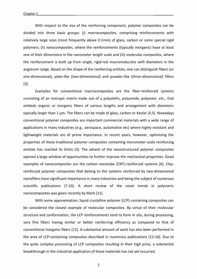
demonstrated by Dencheva et al. [144-147], blending of the components and extruding the

oriented MFC precursors could be performed in a twin-screw extruder coupled with water

baths, heating oven and several cold stretching devices as shown in Figure 1.3.

In the particular case of HDPE/PA6 and HDPE/PA12 precursor materials the

procedures were as follows. Granulates of PA6 or PA12 (pre-dried for 6 h at 100ºC), HDPE

and compatibilizer (a copolymer of HDPE-maleic anhydride (MAH) commercially available

under the name Yparex, YP) were premixed in a tumbler in the desired proportions. Each

mixture was introduced into a gravimetric feeder that fed it into the hopper of a Leistritz

LSM 30.34 laboratory intermeshing, co-rotating twin-screw extruder. The extruder screws

rotated at 100 rpm, and the temperature in its 8 sections was set in the range of 240–250

(for HDPE/PA6) and at 230°C (for the HDPE/PA12 blends). The resulting extrudate was

cooled in the first water bath at 12°C. Meanwhile, the first haul-off unit applied a slight

drawing to stabilize the extrudate cross-section. Further drawing was performed in the

second haul-off unit after the strand passed through the second water bath heated to 97–

99°C. A third haul-off unit applied the last drawing, causing the diameters to decrease from 2

mm (at the extruder die) to approximately 0.6–0.9 mm at the end of the extruder line. Thus,

twelve oriented HDPE/PA/YP blends with compositions given in Table 1.1 were obtained

initially in the form of continuous oriented cables

Extruder Water

Bath 1 Haul-off 1

T = 12ºC

Winder

Cutter

Pelletizer

NOM

MRB

O C

T = 98ºC

2 1 = 2.6

Haul off 2

Hot Air

Oven Haul-off 2 Haul off 3

= 6.3

Figure 1.3 – Schematic representation of the extrusion line used for preparation of polyethylene–polyamide MFC precursors: OC - oriented cable; MRB - middle-length, randomly distributed bristles; NOM - non-oriented material [144]


15

Table 1.1 Composition of the HDPE/PA/YP composites. From each composition UDP, CPC, MRB and NOM composites were produced [146]

These cables were then cut to shape and compression molded at temperature below

the melting point of the respective reinforcing polyamide into three MFC types: (i) in the

form of orthotropic laminae obtained from unidirectional plies of cables (UDP), (ii) cross-ply

laminates (CPC) obtained from two plies of oriented cables arranged perpendicularly, and

(iii) composites from middle-size randomly oriented PA6 bristles (MRB). Compression

molded non-oriented pellets obtained right after extrusion and denoted as “non-oriented

material” (NOM) were also produced from each blend and tested for comparison. Figure 1.4

shows the visual aspect of various types of precursors. Figure 1.4 depicts the preparation of

the CPC laminates from two perpendicularly aligned unidirectional plies of oriented cables

but the form and dimensions are valid for all composite types.

HDPE/PA/YP

composite

designation

HDPE

(wt %)

PA

(wt %)

YP

(wt %)

90/10/0 90.0 10.0 0

80/20/0 80.0 20.0 0

70/20/10 70.0 20.0 10.0

75/20/5 75.0 20.0 5.0

77.5/20/2.5 77.5 20.0 2.5

65/30/5 65.0 30.0 5.0

Figure 1.4.Various MFC precursors obtained after the homogenization and cold drawing stages; (a) OC, oriented cable after the 3rd haul-off; (b) bundles of cut bristles with parallel arrangement; (c) MRB, middle-length randomly distributed bristles; (d) NOM, non-oriented material obtained by palletizing the extrudate before the first haul-off [145]

Chapter 1_____________________ ___________

16

It is worth mentioning that compression molding (CM) is not the only way to

transform the oriented precursors into fibrilar micro- or nanostructured composites.

Chopping the continuous OCs into pellets allows their reprocessing into MFC by extrusion or

by injection molding (IM). This alternative was reported by Monticciolo et al for PE/poly

(butylenes terephthalate) blends [148] and was followed later by other authors [114,128]

with PET/HDPE blends. Both CM and IM matrix isotropization have been used in PET-

reinforced MFCs [12] showing an improvement of the mechanical performance as compared

to that of the pure PA6 matrix. According to this work, the CM approach allowed to stay

more accurately within the necessary processing temperature window and to preserve

better during the isotropizaton stage the microfibrillar morphology of PET. For this reason,

the mechanical properties in impact and flexural mode were better. On the other hand, one

should bear in mind that in contrast to CM it IM cannot produce laminates with continuous

and parallel reinforcing fibrils where the advantages of the MFC technology are most

obvious.

A possibility to avoid the CM stage is offered by the modified method for preparation

of in situ MFCs based on consecutive slit or rod extrusion, hot stretching and quenching

[114,119,120,125,129] used to process thermoplastic polymer blends, mostly polyolefins and

PET. Rotational molding of LDPE/PET beads has also been attempted for the same purpose

[107], but the reinforcing effect was insufficient due to the uneven distribution of the

reinforcing fibrils and also due to their reversion to spheres.

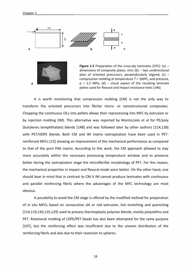
Figure 1.5 Preparation of the cross-ply laminates (CPC): (a) -- dimensions of composite plates, mm; (b) -- two unidirectional plies of oriented precursors, perpendicularly aligned; (c) – compression molding at temperature T = 160ºC, and pressure, p = 1,5 MPa; (d) – visual aspect of the resulting laminate plates used for flexural and impact resistance tests [146]


17

An interesting further development of the MFC preparation concept is found in [149].

A PP/PET blend is prepared by melt extrusion which is thereafter spun into textile synthetic

fibers followed by knitting or weaving and the obtained fabric is compression molded below

the melting points of the two components. Apart from the observed 30-35% increase of the

Young’s modulus and tensile strength, which is typical for the MFC systems, the authors

describe the preparation of nanofibrillar fabrics by means of a simple selective dissolution of

the matrix PP with possible applications for scaffolds and single-polymer composites.

1.3.2. Mechanical characterization of PE/PA microfibrilar composites

It is generally accepted [19] that the mechanical properties of the MFC with

optimized composition made under best processing conditions are superior to those of the

corresponding neat matrix material due to the high AR of the crystalline and oriented

microfibrilar reinforcement, and in view of the various possibilities to strengthen the matrix–

fibril interface by compatibilization or transcrystallization. Similar results were obtained with

the two groups of MFC materials – capable and incapable of self-compatibilization.

Thus, MFCs based on self-compatibilizing mixtures of PA6 (matrix) and PET, PBT or

PA66 as reinforcement component, taken in various weight ratios, show a drastic increase of

the tensile strength and of the Young’s modulus values, E , after drawing of the extrudate.

The values reach those of the reinforcing component, e.g. PET, PBT or PA66, when in the

drawn state [19,104]. Subsequent isotropization by compression or injection molding results

in either a slight (for E ) or strong (for σ) decrease. However, the properties of the MFC

are still undoubtedly better than those of the neat matrix and about the same or slightly

better than those of the GF-reinforced polyamide (PA6 + 30% GF). The values of the MFCs

are by 30–40% higher than the rule-of-mixture values calculated from the properties of the

individual components, e.g. isotropic PA6 and drawn PET [103]. This indicates a mechanical

property profile with a clear synergistic effect. It is important to note that the mechanical

properties of PET/PA6 composites are highly dependent on the way the isotropization was

achieved: by IM or CM. Apparently, in both IM and CM cases, the MFCs show a major

improvement of the mechanical performance as compared to that of the pure PA6 matrix.

Depending on the mode of oriented blend isotropization, the values of the MFCs could

be comparable to or even higher than those of the glass-fiber-reinforced matrix. The notable

differences in the E and σ values for IM and CM methods are apparently related to the

Chapter 1_____________________ ___________

18

different morphology of the PET/PA6 MFCs. The CM approach allows one, in contrast to IM,

to stay accurately within the necessary processing temperature window so as to preserve

during the isotropization stage the microfibrilar morphology of PET [12].

As to the MFC composites incapable of self-compatibilization, systematic mechanical

studies were made first with systems based on polyolefin matrices reinforced by PET

microfibrils and very recently - for PE/PA MFC systems. Thus, MFC obtained from LDPE/PET

oriented blends selectively isotropized by injection molding achieved elastic moduli

approaching those of LDPE + 30% glass fibers (GF). The tensile strength of MFC has reached

at least two times that of the neat LDPE matrix material, the impact strength of the MFC

being 50% higher [112]. Extensive mechanical studies have also been performed with the

PP/PET [114,128] and HDPE/PET MFC [116,151]. The tribological properties of polyolefin

matrices reinforced by PET or PA66 were also studied [152]. It was established that the

reinforcement with PA66 fibrils leads to higher wear resistance in comparison to PET in MFC

with the same matrix material. The wear rates were found to be much lower in MFC with

uniaxialy oriented reinforcing fibrils as compared to materials with random orientation of

the reinforcements.

In an attempt to explain better the mechanical properties of MFCs and to enable

their theoretical prediction, Fuchs et al. [124] tested the extent of the validity of the Tsai–Hill

equation applied to MFCs, in which the reinforcing elements represent microfibrils with

diameters around 1 µm and aspect ratios of approximately 100. The commonly used Tsai–

Hill equation has the following form:

2

1

2

22

2

4

2

222 sincossin)sin(coscos

SYXx (1)

wherein x is the tensile strength at a given angle ; X and Y are the tensile strengths in the

fiber and transverse directions, respectively, S is the shear strength and is the off-axis test

angle. Compression-molded plates of PP/PET MFC were prepared and their structures were

established by WAXS and SEM analyses. The tensile tests of cut specimens at various angles

with respect to the uniaxially aligned microfibrils showed the degree of agreement with the

predictions of equation 1. The measured values were slightly higher than the calculated ones

and this finding was explained by the higher aspect ratios of microfibrils, their

more homogenous distribution and, most importantly, by the better matrix–reinforcement


19

adhesion in the case of MFCs as compared to the common composites. The fracture

mechanism as determined from the SEM observations of the fracture surfaces was also

discussed and a good agreement with the mechanical behavior was found.

Recently, the mechanical behavior of HDPE/PA6 MFC, with and without

compatibilization, was studied by Dencheva et al [147]. The composites were produced by

conventional processing techniques in the form of UDP, CPC, MRB or NOM. Depending on

the PA6 and YP amounts, the UDP, CPC and MRB materials showed better mechanical

performance than the HDPE matrix in terms of their tensile, flexural and impact properties.

20% of PA6 reinforcement seems to be the optimal concentration. A fibrilar morphology of

the PA6 reinforcement was needed for major improvement of all mechanical properties. In

composites with fibril reinforcement (UDP, CPC, and MRB) the Yparex compatibilizer has a

negative effect on the mechanical properties in tensile, flexural and impact modes. In NOM

where the reinforcement is globular the effect is reversed. More about the sample

preparation and the proper testing will be mentioned in the Experimental part, since in this

thesis the testing methodology and data handling of [147] were adopted.

1.3.3 Morphology and structure investigations of MFCs

The changes occurring in both matrix and reinforcing components during MFC

preparation may be followed by different methods, of which most frequently electron

microscopy (SEM and TEM) and X-ray techniques are used.

The first extensive SEM investigation of PET/PA6- based MFCs and their precursors

performed by Evstatiev et al [152] undoubtedly showed the fibrilar structure of the PET

reinforcements preserved after the PA6 matrix isotropization. Since then,

electron microscopy has been used to visualize the orientation and morphology of the matrix

and reinforcing components in almost every report on MFCs. It is worth noting some more

recent studies on MFCs comprising low-density polyethylene (LDPE) and PET as matrix and

reinforcement, respectively [112,113]. Several microscopic techniques were used, e.g.

SEM, polarized light microscopy (PLM) and TEM. Thus, by SEM it was demonstrated that the

isotropic LDPE matrix embedded PET microfibrils with random orientation. PLM and TEM of

thin slices showed the orientation in the machine direction. The latter method revealed

also the formation of transcrystalline layers of LDPE on the oriented PET microfibrils. Similar

investigations were performed by Li et al. [154] by means of SEM and AFM. As seen from

Chapter 1_____________________ ___________

20

Figure 1.6 the authors visualized the transcrystalline morphology of PET/iPP MFCs. On this

basis, a shish-kebab model was proposed. Microfibrils containing blends of polycarbonate

(PC) and HDPE were also produced and characterized by SEM thus proving the presence of

PC fibrils in the polyolefin matrix [115].

Figure 1.6 AFM phase image of the cryogenic cut surfaces of an as-stretched microfibrilar PET/iPP (15/85 by weight) MFC showing the transcrystalline layers and the shish-kebab structure: A, the shish of iPP; B, the kebab of iPP induced by iPP shish; C, the kebab of iPP induced by PET microfibrils [153].

Some PLM and SEM images of HDPE/PA12 UDP MFCs were performed in [144]. The

PLM micrographs taken at 130°C (i.e., above matrix Tm) demonstrated that the PA12

component continues to be in the form of crystalline fibrils and are concentrated in the

middle (‘core’) zone of the specimen. They remain oriented in the longitudinal

direction, while in the ‘shell’, i.e. closer to the sample surface, there seem to be a higher

concentration of HDPE material being molten at this temperature. The SEM study gave more

details of the morphology suggesting that in the non-compatibilized MFCs the fibrils are

poorly linked to the HDPE matrix while in the presence of YP second the reinforcing

elements are tightly embedded within the matrix. SEM micrographs very similar those in

[154] were obtained by Boyaud et al with various MFC-like systems reinforced by PBT fibers

[155, 156].

Systematic morphology investigations on HDPE/PA6/YP and HDPE/PA12/YP MFC

systems have been described in [145,146]. The evolution of morphology in the UDP

materials (e.g., their visible diameters, lengths and aspect ratios) was followed during the

various processing stages as a function of the blend composition by means of electron

microscopy and synchrotron X-ray scattering techniques. It was demonstrated that right

after the extruder die, the PA exist in the form of globules embedded in an isotropic HDPE.

During the cold drawing stage, i.e., in the oriented precursor cables, both HDPE and PA are


21

fibrillated. During the compression molding at 160°C, the HDPE fibrils melt and upon the

subsequent cooling and crystallization of the matrix, the PA fibrils are coated with a

transcrystalline layer (TCL) of matrix material. A method was developed for estimation of the

real AR of the PA fibrils based on the selective dissolution of the TCL. The influence of the

compatibilizer content on the TCL thickness and structure as well as on the other

morphological characteristics of the composites was assessed. Based on the SEM and TEM

studies in [145,146], a model was suggested visualizing the structural changes during the

MFC preparation.

As far as X-ray techniques are concerned, WAXS, SAXS are frequently employed for

structural investigations of transcrystallinity in conventional and nanostructured fiber

composites. Thus, Feldman et al.[157] studied the structural details of PA66 transcrystallinity

induced by the presence of aramid (Kevlar 29, 49 and 149) and carbon (pitch based) fibers,

as determined by high resolution synchrotron WAXS. The main observation was that the

orientation was distinct for each system and almost independent of distance from the fiber.

In an earlier X-ray diffraction study of aramid and carbon fiber-reinforced PA66, it was

concluded that in the nucleation and initial growth stages the first chain folds were oriented

so that the chain axis was aligned in the fiber direction, and in the crystal growth that

followed a typical sheaf structure was formed (described graphically in [157]), leading

gradually to spherulite formation, as in bulk crystallization [158]. WAXS analysis performed

on PE-fiber-reinforced HDPE matrix [159,160] revealed that the TCL was grown on the fiber

surface originating from matrix material with properties depending on the processing

conditions. Banded transcrystalline morphology developed under ice-water quenching and

air cooling conditions, whereas under isothermal crystallization an apparent rod-like

morphology was observed to develop in the matrix. Additional examples for transcrystallinity

investigation by X-ray techniques are pointed out in the excellent review of Quan et al on

transcrystallinity in polymer composites [162] revealing the state-of-the-art in the area until

2005.

More recently, polymer transcrystallinity induced by CNT in PP matrices was studied

by Zhang et al [163]. It was concluded that supramolecular microstructures of PP

transcrystals induced by the nanotube fiber are observed in the range of isothermal

crystallization temperatures from 118°C to 132°C. WAXS analyses have shown that the

nanotubes can nucleate the growth of both α- and γ-transcrystals, whereby the α-

Chapter 1_____________________ ___________

22

transcrystals dominated the overall interfacial morphology. Also, close to the nanotube fiber

surface, a cross-hatched lamellar microstructure composed of mother lamellae and daughter

lamellae has been observed. As far as other advanced X-ray scattering studies in polymer

composites are concerned, it is worth mentioning also the study of Hernández et al [164].

The relationships between the macroscopic deformation behavior and microstructure of a

pure poly(butylene terephthalate)-block-poly(tetramethylene oxide (PBT-b-PTMO) block

copolymer and a polymer nanocomposite (PBT-b-PTMO) containing 0.2 wt% single wall CNT

were investigated by simultaneous synchrotron SAXS and WAXS during tensile deformation.

The structural data allowed the conclusion that the CNT acted as anchors in the

nanocomposite, sharing the applied stress with the PBT crystals and partially preventing the

flexible, non-crystallisable PTMO chains to elongate.

In HDPE/PA MFCs X-ray studies were also applied and especially in [144,145]. These

systematic investigations of the nanostructure of HDPE/PA6/YP and HDPE/PA12/YP UDP

materials by synchrotron SAXS and WAXS became the initial point of the studies in this

thesis. The method for the TCL investigation based on WAXS was adopted in this work and

will be explained in detail in the Experimental part.

The main outcome of the nanostructure research of HDPE/PA/YP MFCs was the

possibility to relate the thickness and morphology of the TCL with the mechanical properties

of the MFC materials with either PA6 or PA12 fibril reinforcement. Thus, in HDPE/PA6/YP

UDP MFCs, compatibilization resulted in thinner and shorter fibrils in which both the PA6

core and the HDPE TCL were finer. The significantly lower AR in the YP containing HDPE/PA6

composites drastically decreased the tensile and impact strength in respect to the non-

compatibilized composite, but the flexural stiffness was almost unaffected. As regards the

PA12 reinforced MFCs, again the best mechanical properties were related with the highest

AR values. Interestingly, the tensile and flexural properties of the 80/20/0 PA12-reinforced

composite were notably better than of the PA6-analogue. This effect is probably due to the

significantly thinner TCL in the PA12-reinforced MFC. This thinner HDPE coating affects less

negatively the way the load is transferred from the matrix to the PA12 reinforcing fibrils,

especially if the AR remains constant.

Concluding the discussion on the structural studies of MFCs, one has to mention some

additional analytical methods used for their investigation that are related to the mechanical

properties. Dynamic mechanical thermal analysis (DMTA) was employed for


23

PET/PA6 composites focusing mainly on the changes in the amorphous phase [165]. This

method enables one to distinguish the effects of self-compatibilization of the blend during

the various stages of MFC preparation. Interestingly enough, drawing of the PET/PA6

blend induces some measurable compatibilization effect. Annealing below 220°C resulted in

reorganization of the PET and PA6 homopolymers within distinct phases revealing the

inherent immiscibility of this blend. Only prolonged heat treatment above this temperature

produced compatibilization at the interface.

DMTA investigations of a LDPE/PET system [166] by three-point bending in the -20 to

+100°C range demonstrated that the MFCs displayed complex modulus E* values more than

10 times higher than those of neat LDPE. In addition, the E* values obtained in dynamical

mode were quite close to the values of the Young’s modulus measured in static

conditions demonstrating in a fine way the reinforcing effect of the microfibrils in MFCs.

Microhardness measurements are an additional possibility for monitoring the structure

development in PET/PA6 blends during their transformation into MFCs [167]. The results

obtained showed a linear correlation of the elastic modulus anisotropy and

the microindentation hardness anisotropy in all oriented samples studied. Moreover, the

indentation modulus values in the blends followed the parallel additivity model of the

individual components. The use of the additivity law led to the determination of the

modulus of the PET microfibrils within the MFC, otherwise inaccessible from direct

measurements.

1.4 Research goals and structure of the thesis

From the above literature survey it can be inferred that among the various types of

polymer materials the clay-reinforced nanocomposites and the in-situ microfibrilar

composites deserve special attention. In general, the MFC technology combines the

strong points of conventional fibrous composites, the LCP and nanoclay - reinforced polymer

systems, avoiding some of their most important limitations. Hence, the MFCs are materials

with controlled heterogeneity obtainable by conventional processing techniques such as

extrusion, compression molding or injection molding, with no agglomeration of the

reinforcing phase. On the other hand, the PA/o-MMT nanocomposites have been

investigated in great detail and already gained industrial importance. Their major limitation

is the agglomeration of the reinforcements occurring during processing when extrusion or

Chapter 1_____________________ ___________

24

injection molding is used. The main idea of this thesis is to try to obtain MFC materials in

which the reinforcing, in-situ obtained fibrils are additionally reinforced by nanosized MMT

filler, thus combining the useful properties of both MFC and clay reinforced nanocomposites.

Among the numerous polymers that are reportedly used for matrices of MFC, HDPE

deserves special attention because it is a polymer of major production scale and importance,

with very good mechanical properties and relatively low melting temperature. Therefore, it

is very suitable as matrix material in the MFC technology, as proved by the extensive recent

studies dedicated to HDPE/PA MFCs. Polyamides possess excellent mechanical properties,

are semicrystalline with relatively high melting temperatures (but lower than that of PET),

easily form fibers by drawing, and are capable of chemical interactions with HDPE in the

presence of suitable compatibilizers. Most importantly, polyamides, in particular PA6, have

been widely used in clay nanocomposites obtaining materials with excellent mechanical

properties. Therefore, it was decided to work in the field of MFCs based on HDPE matrix

reinforced by PA6, the latter representing o-MMT-filled nanocomposites, using as

compatibilizer a commercial polymer of maleic anhydride grafted polyethylene (Yparex, of

DSM).

The initial research program was based on the following stages:

- Preliminary study of the structure and mechanical properties of PA6 modified with

different amounts of two different nanoclay types: Cloisite 15A o-MMT and a

Nanomer/PA6 concentrate containing 20 wt % of clay.

- Preparation of highly oriented precursors from HDPE/PA6-clay/Yparex blends by

extrusion, varying the type of PA and composition of the blend. In these blends the

PA6 is reinforced by either Cloisite or Nanomer clay taken in an optimized amount;

- Preparation of clay-containing MFCs with an isotropic matrix by compression molding

varying the length and alignment of the oriented precursors;

- Characterization of the mechanical behavior of the clay-containing MFCs for studying

the influence of the blend composition, fibril geometry and alignment on the

properties;

- Study of the morphology and structure of the clay-containing MFCs for establishing

the composition-structure-properties relationship.


25

In the process of the investigation, additional goals emerged and were achieved, such

as structure-properties relation by simultaneous synchrotron-stretching experiments, FT-IR

microscopy studies for a multiscale characterization of the MMT distribution, etc.

Figure 1.7 demonstrates the different pieces of the thesis:

Figure 1.7 The structure of this thesis

Development and Investigation of New Hybrid Composite Materials Based on Oriented Blends of Thermoplastic Polymers

and Nanosized Inorganic Fillers

Conclusions

Experimental processing and analytical methods used for study of the precursors and MFCs in this thesis Chapter 2

Formulation of the main research topics and goals: HDPE/PA6/YP MFCs additionally reinforced by nanoclays Chapter 1

Relationship between the mechanical properties and the nanostructure in oriented precursors for MFCs, based on

simultaneous straining/synchrotron SAXS experiments Chapter 4

Structure-properties relationship in montmorillonite-filled polyamide 6 nanocomposites Chapter 3

Investigation of the mechanical properties in tensile, flexural and impact modes of HDPE/PA6-MMT/YP composites Chapter 5

Literature study on PA6/MMT composites: production, charac- terrization, morphology, nanostructure, properties. Chapter 1

Literature study on MFC systems: preparation, analytical methods, morphology and structure, properties. Chapter 1

Structure-properties relationship in HDPE/PA6-MMT/YP composites by means of synchrotron SEM, WAXS and SAXS Chapter 6

Future Work

Chapter 1_____________________ ___________

26

1.5 References

1. Schadler L S (2003), Polymer-based and Polymer-filled Nanocomposites in Nano-

composite Science and Technology, (Eds. Ajayan P M, Schadler L S and Braun P V), pp.

77-144.

2. Early JW, Osthaus BB, and Milne IH (1953), Amer. Mineral. 38: 707-724.

3. Grim E, Ralph E and Kulbicki G (1961), Amer. Mineral. 46: 1329-1369.

4. Thostenson ET, Ren Z and Chou TW (2001), Composites Science and Technology 61:

1899–1912.

5. Jang BZ (1992), Composites Science and Technology 44:333-349.

6. Pulickel AM and Otto ZZ (2001) Topics in Applied Physics 80:391-495.

7. Usuki A, Kojima Y, Kawasumi M, Okada A, Fukushima Y, Kurauchi T and Kamigato O

(1993), J Mater Res 8:1179-1184.

8. Yano K, Usuki A, Okada A, Kurauchi T and Kamigaito O (1993), J Polym Sci A: Polym

Chem 31:2493-2498.

9. Giannelis EP (1998), Appl Organomet Chem 12:675-680.

10. Ray S S and Okamoto M (2003), Prog Polym Sci 28:1539-1641.

11. Mark JE (2006), Acc Chem Res 39:881-887.

12. Evstatiev M, Fakirov S, Bechtold G and Friedrich K (2000), Adv Polym Technol 19:249-

259.

13. Chakraborty S, Sahoo NG, Jana GK and Das CK (2004), J Appl Polym Sci 93:711-718.

14. Tjong SC (2003) Mater Sci Eng 41:1-60.

15. Song CH and Isayev AI (2001), Polymer 42:2611-2619.

16. Handlos AA and Baird DG (1996), Int Polym Proc 11:82-93.

17. Evstatiev M and Fakirov S (1992), Polymer 33:877–880.

18. Evstatiev M, Fakirov S and Schultz, J M (1993), Polymer 34:4669–4679.

19. Fakirov S, Evstatiev M and Friedrich K (2002), Nanostructured Polymer Composites

from Polymer Blends: Morphology and Mechanical Properties in Handbook of

Thermoplastic Polyesters, (Ed. Fakirov S.), Wiley-VCH, Weinheim Germany, pp the-

1132.

20. Schaefer D W and Justice R S (2007), Macromolecules 40:8501–8517

21. Fornes T D, Yoon P J, Keskulla H and Paul D R (2002), Polymer 43: 5915.

22. Tjong S C and Bao S P (2004), J Polym Sci: Part B: Polym Phys 42: 2878.


27

23. Fornes T D, Hunter D L and Paul D R (2004), Polymer 45: 2321.

24. Gilman J W (1999), Appl Clay Sci 15: 31.

25. Giannelis E P (1998), Appl Organomet Chem 12: 675.

26. Kojima Y, Usuki A, Kawasumi M, Okada A, Kurauchi T and Kamigaito O (1993), J

Polym Sci Part A: Polym Chem 31: 983.

27. Kojima Y, Usuki A, Kawasumi M, Okada A, Kurauchi T and Kamigaito O. (1993), J

Polym Sci Part A: Polym Chem 31: 1755.

28. Gilman JW, Jackson CL, Morgan AB, Harris R. , Manias E, Giannelis EP, Wuthenow M,

Hilton D and Philips SH (2000), Chem Mater 12: 1866.

29. Gilman J W, Kashiwagi T and Lichtenhan J D (1999), SAMPE J 33: 40.

30. Yano K, Usuki A, Okada A, Kurauchi T and Kamigaito O (1993), J Polym Sci Part A:

Polym Chem 31: 2493.

31. Yano K, Usuki A and Okada A (1997), J Polym Sci Part A: Polym Chem 35: 2289.

32. Avella M, Bondioli F, Cannillo V, Di Pace E, Errico M E, Ferrari A M, Focher B and

Malinconico (2004), M. Compos Sci Technol 66: 886.

33. Osman M A Ploetze M and Skrabal P (2004), J Phys Chem B108: 2580.

34. Ross C S and Hendrics S B (1945), US Geological Survey Prof Paper No.205B.

35. Fischer H (2003), Materials Science and Engineering 23: 763–772.

36. Utracki L A, Sepehr M and Boccaleri E (2007), Polym Adv Technol 18: 1–37.

37. Sinha Ray S, Okamoto K and Okamoto M (2003), Macromolecules 36: 2355.

38. Usuki A, Kawasumi M, Kojima Y, et al. (1993), J Mater Res 8(5): 1179-1184.

39. Mc Atee J L (1962), Clay Minerals 9: 444-450.

40. Ton-That M-T, Perrin-Sarazin F, Cole K C, Bureau M N and Denault J (2004), Polym

Eng Sci 44: 1212–1219.

41. Gilman J W (1999), Appl Clay Sci 15(1-2): 31–49.

42. Lan T and Pinnavaia T (1994), Chem Mater 6: 2216–2219.

43. Bolton EK (1942), Ind Eng Chem 34: 53.

44. Mc Atee J L (1962), Clay Minerals 9: 444-450.

45. Aharoni S M (1995), n-Nylons: Their Synthesis, Structure and Properties, John Wiley

& Sons, Chichester, M.I. Kohen, Nylon Plastics Handbook, Hanser, New York.

46. Usuki A, Hasegawa and Kato M (2005), Advanced polymer science 179: 135-195.

Chapter 1_____________________ ___________

28

47. Utracki LA (2004), Clay-containing Polymeric Nanocomposites, vol. 1 & 2. RAPRA:

Shawbury, UK.

48. Fujiwara S and Sakamoto T (1976) Japanese patent No JPA51- 109998, Unitika Ltd

49. Fujiwara S and Sakamoto T (1975),“Method for manufacturing a clay-polyamide

composite”, Japan Kokai, 109, 998.

50. Kamigaito O Fukushima Y and Doi H, US. Patent, 4, 472, 538, 18.09.1984 Toyota

51. Okada A, Fukushima Y, Kawasumi M, Inagaki S, Usuki A, Sugiyama S, Kurauchi K, and

Kamigaito O, U.S. 4739007 (1988), Toyota Motor Co.

52. Fukushima Y, Okada A, Kawasumi M, Kurauchi T and Kamigaito O (1988), Clay

Minerals 23: 27-34.

53. Usuki A, Kojima Y, Kawasumi M, Okada A, Kurauchi T and Kamigaito O (1990),

Polymer 31: 651-652.

54. Kojima Y, Youshitsugu T, Usuki A , Animitsu K, Kawasumi M, Masaya A, Okada

A, Kurauchi T and Kamigaito O (1993), J Polym Sci Part A: Polym Chem 31: 983-986.

55. Kojima Y, Youshitsugu T, Usuki A, Animitsu K, Kawasumi M, Masaya A, Okada A,

Kurauchi T and Kamigaito O (1993), Journal of Applied Polymer Science 49:683-687.

56. Kojima Y, Youshitsugu T, Usuki A, Animitsu K, Kawasumi M, Masaya A, Okada A,

Kurauchi T and Kamigaito O (1994), J Polym Sci Part Part B: Polym Phys 32: 625-630.

57. Usuki A, Koiwai A, Kojima Y, Kawasumi M, Okada A, Kurauchi T, Kamigaito O (1995), J

Appl Polym Sci 55: 119-123.

58. Maxfield M R, Christiani B R, Murthy S N and Tuller H., US. Patent, 5, 385, 776,

31.01.1995, Allied Signal

59. Masenelli-Varlot K, Reynaud E, Vigier G and Varlet J (2002), J Polym Sci Part Part B:

Polym Phys 40: 272–283.

60. Ma C M, Kuo C T, Kuan H C and Chiang C L (2003), J Appl Polym Sci 88: 1686–1693.

61. Rauwendaal C (2001), "Polymer extrusion", 4th edition, Hanser Gardner Publications,

Munich, Germany.

62. Shelley J S, Mather P T, and DeVries K L (2001), Polymer 42: 5849-5858.

63. Derek M, Lincoln T and Vaia R A (2004), Macromolecules 37: 4554-4561.

64. Avlar S and Qiao Y (2005), Composites: Part A 36: 624–630.

65. Vlasveld D P N, Groenewold J, Bersee H N, S and Picken S J (2005), Polymer 46:

12567–12576.


29

66. Yang K and Ozisik R (2006), Polymer 47: 2849–2855.

67. Wilkinson A N, Man Z, Stanford J L, Matikainen P, Clemens M L, Lees M S, and Liauw

C M (2007), Composites Science and Technology 67: 3360–3368.

68. Fornes T D , Yoon P J , Keskulla H and Paul D R (2001), Polymer 42: 9929-9940.

69. Fornes T D , Yoon P J , Keskulla H and Paul D R (2002), Polymer 43, 5915–5933.

70. Xie S, Zhang S, Liu H, Chen G, Wang F and Yang M (2005), Polymer 46: 5417–5427.

71. Yuan M, and Turng S (2005), Polymer 46: 7273–7292.

72. Lincoln D M, Vaia R A , Wang Z G and Hsiao B S (2001), Polymer 42: 1621–1631.

73. Lincoln D M, Vaia R A , Wang Z G, Hsiao B S and Krishnamoorti R (2001), Polymer 42:

9975-9985.

74. Lincoln D M and Vaia R A (2004), Macromolecules 37: 4554-4561.

75. Dennis H R , Hunter D L, Chang D, Kim S, White J L, Cho J W and Paul D R (2001),

Polymer 42: 9513-9522.

76. Varlot K, Reynaud E, Kloppfer K H, Vigier G and Varlet J (2001), J Polym Sci Part Part

B: Polym Phys 39: 1360–1370.

77. Ibanes C, de Boissieu M, David L and Seguela R (2006), Polymer 47: 5071–5079.

78. Li L, Bellan L M, Craighead H G and Frey M W (2006), Polymer 47: 6208-6217.

79. Fong H, Liu W, Wang C-S, Vaia R A (2002), Polymer 43: 775-780,

80. Ibanes C, David L, de Boissieu M, Seguela R Epicier and Robert G (2004), J Polym Sci

Part Part B: Polym Phys 42: 3876–3892.

81. Ibanes C, David L, Seguela R, Rochas C and Robert G (2004), J Polym Sci Part Part B:

Polym Phys 42: 2633–2648.

82. Hasegawa N, Okamoto H, Kato M, Usuki A and Sato N (2003), Polymer 44: 2933–

2937.

83. Fedullo N, Sclavons M, Bailly C, Lefebre J M and Devaux J (2006), Macromol Symp

233: 235–245.

84. Bertmer M, Wang M, Kruger M, Blumich B, Litvinov V and van Es M (2007), Chem

Mater 19: 1089.

85. Liu X and Wu Q European Polymer Journal (2002), 38: 1383–1389.

86. Shelleya J S, Matherb P T and DeVries K L (2001), Polymer 42: 5849-5858.

87. Kamal M R, Borse N K and Garcia-Rejon A (2002), Polym Eng and Sci 42: 9.

88. Loo L S and Gleason K K (2004), Polymer 45: 5933–5939.

Chapter 1_____________________ ___________

30

89. Davis R D, Gilman J W and van der Hart D L (2003), Polymer Degradation and

Stability 79: 111–121.

90. Devaux S, Bourbigot S and El Achari A (2002), J Appl Polym Sci 86: 2416–2423.

91. Fermeglia M, Ferrone M and Pricl S (2003), Fluid Phase Equilibria 212: 315–329.

92. Shenga N, Boycea M C, Parksa D M, Rutledgeb G C, Abesb J I and Cohen R E (2004),

Polymer 45: 487–506.

93. Kim G M, Lee D H, Hoffmann B, Kressler J and Stoppelmann G (2001), Polymer 42:

1095-1100.

94. Mederic P, Razafinimaro T, Aubry T (2006), Polym Eng and Sci 46:986-994.

95. Liu X, Wu Q and Berlung L A (2002), Polymer 43:4967–4972.

96. Chavarria F and Paul D R (2004), Polymer 45:8501–8515.

97. Kang X, He S, Zhu C, Lu L W L and Guo J (2005), J Appl Polym Sci 95: 756–763.

98. Zhang Y, Yang J H, Ellis T S and Shi J (2006), J Appl Polym Sci 100: 4782–4794.

99. Hedicke K., Wittich H, Mehler C, Gruber F and Altstadt V (2006), Compos Sci Technol

66: 571–575.

100. Denchev Z. and Dencheva N (2008), Polym Int 57:11–22.

101. Fakirov S, Evstatiev M and Friedrich K (2000), Polymer Blends, vol. 11, (Eds. Paul D R

and Bucknall C B), Wiley, New York, pp. 455–476.

102. Fakirov S, Evstatiev M and Friedrich K (1998) Microfibrillar reinforced composites from

polymer blends, in Polymerwerkstoffe 1998: Verarbeiterung, Anwendung, Recycling,

(Eds. Radusch HJ and Vogel J), Martin-Luther-Universitȁt, Halle-Wittenberg,

Halle/Saale, p. 123-156.

103. Evstatiev M, Fakirov S and Shultz J M (1993), Polymer 34: 4669-4679.

104. Evstatiev M, Fakirov S and Friedrich K (2005), Manufacturing and characterization of

microfibrillar reinforced composites from polymer blends. In Polymer Composites:

From Nano- to Macroscale; Friedrich, K., Fakirov, S., Zhang, Z., Eds.; Springer: New

York, 149–167

105. Shields R J, Bhattacharyya D and Fakirov S (2008), J Mater Sci 43: 6758–6770.

106. Denchev Z, Evstatiev M, Fakirov S, Friedrich K and Pollio M (1998), Adv Comp Mater

7: 313-324.

107. Lin R J T, Bhattacharyya D and Fakirov S (2007), Key Eng Mater 334–335:349.

108. Denchev Z, DuChesne A, Stamm M and Fakirov S (1998), J Appl Polym Sci 68: 429-440.


31

109. Denchev Z, Bojkova A, DuChesne A, Hȍcker H, Keul H and Fakirov S (1998), Macromol

Chem Phys 199: 2153-2164.

110. Fakirov S, Kamo H, Estatiev M and Friedrich K (2005), J Macromol Sci: Part B Phys B43:

775–89.

111. Friedrich K, Ueda E, Kamo H, Evstatiev M, Krasteva B and Fakirov S (2002), J Mater Sci

37: 4299-4305.

112. Li Z M, Yang M B, Lu A, Feng J M and Huang R (2002), Mater Letters 56: 756–762.

113. Li Z M, Yang M B, Huang R, Yang W and Feng J M (2002), Polym Plast Technol Eng 41:

19–32.

114. Lin R J T, Bhattacharyya D and Fakirov S (2007), Key Eng Mat 334: 349–352.

115. Xu HS, Li Z M, Wang S J and Yang MB (2007), J Polym Sci Part B: Polym Phys 45: 1205–

1216.

116. Li Z M, Xie B H, Huang R, Fang X P and Yang M B (2004), Polym Eng Sci 44: 2165–2173.

117. Li Z M, Yang W, Xie B-H, Huang R and Yang M-B (2004), Macromol Mat Eng 289: 349–

354.

118. Li Z M, Li L B, Shen K Z, Yang M B and Huang R (2004), J Polym Sci Part B: Polym Phys

42: 4095–4106.

119. Zhong G J, Li Z M, Li L B, and Mendes E (2007), Polymer 48: 1729–1740.

120. Jayanarayanan K, Thomas S and Joseph K (2008), Composites Part A 39: 164–175.

121. Friedrich K, Evstatiev M, Fakirov S, Evstatiev O, Ishii M and Harrass M (2005), Compos

Sci Technol 65: 107–116.

122. Li Z M, Yang W, Li L-B, Xie B-H, Huang R and Yang M-B (2004), J Polym Sci Part B: Polym

Phys, 42: 374–385.

123. Li Z M, Li L-B, Shen K-Z, Yang W, Huang R and Yang M-B (2004), Macromol Rapid

Commun 25: 553–558

124. Fuchs C, Bhattacharyya D and Fakirov S (2006), Compos Sci Technol 66: 3161–3171.

125. Karingamanna J, Sabu T and Kuruvilla J (2010), J Polym Res DOI 10.1007/s10965-009-

9384-6 (2010).

126. Evstatiev M, Fakirov S, Krasteva B, Friedrich K, Covas JA and Cunha AM (2002), Polym

Eng Sci 42: 826–835.

127. Taepaiboon P, Junkasem J, Dangtungee R, Amornsakchai T and Supaphol P (2006), J

Appl Polym Sci 102: 1173–1181.

Chapter 1_____________________ ___________

32

128. Lei Y, Wu Q, Xu Y and Yao F (2009), Composites Part A 40: 904–912.

129. Chatreenuwat B, Nithitanakul M and Grady B P (2007), J Appl Polym Sci 103: 3871–

3881.

130. Lin C, Sun H, Wang S, Huang J, Li J and Guo S (2010), J Appl Polym Sci 116: 320–327.

131. Kamal M R, Jinnah I A and Utracki L A (1984), Polym Eng Sci 24: 1337-1347.

132. Beltrame, P L, Castelli A, Pasquantonio M D, Canetti M and Seves A (1996), J Appl Polym

Sci 60: 579-590.

133. Yeh J T, Huang S S and Chen H Y (2005), J Appl Polym Sci 97: 1333-1344.

134. Willis J M and Favis B D (1988), Polym Eng Sci 28: 1416-1426.

135. Chandramouli K and Jabarin S A (1995), Adv Polym Technol 14: 35-46.

136. Utracki L A, Dumoulin M M and Toma P (1986), Polym Eng Sci 26: 34-44.

137. R. Steward (2004), Plast Eng 60: 23.

138. Wouters M E L, Litvinov V M, Binsbergen F L, Goossens J G, van Duin M and Dikland H G

(2003), Macromolecules 36: 1147-1156.

139. Filippi S, Chiono V, Polacco G, Paci M, Liliya I, Minkova L and Magagnini P (2003),

Macromol Chem Phys 203: 1512–1525.

140. Burger C, Hsiao B S and Chu B (2006), Annu Rev Mater Res 36: 333-368.

141. Fakirov S, Evstatiev M and Petrovich S (1993), Macromolecules 26:5219-5226.

142. Evstatiev M, Schulz J M, Georgiev G, Petrovich S, Fakirov S and Friedrich K (1998), J Appl

Polym Sci. 67:723-737.

143. Fakirov S and Evstatiev M (1994), Adv Mater 6:395-398.

144. Denchev Z, Oliveira MJ and Carneiro OS (2004), J Macromol Sci Phys B43:143-162.

145. Dencheva N, Oliveira M J, Carneiro O S, Pouzada A S and Denchev Z (2010), J Appl Polym

Sci 115:2918–2932.

146. Dencheva N, Denchev Z, Oliveira M J and Funari S S (2010), Macromolecules 43:4715-

4726.

147. Dencheva N, Oliveira M J, Pouzada A S, Kearns M and Denchev Z (2010), Mechanical

properties of polyamide 6 reinforced microfibrillar composites, Polym Comp (in press).

148. Monticciolo A, Cassagnau P and Michel A (1998), Polym Eng Sci 38: 1882.

149. Shenga N, Boycea M C, Parksa D M, Rutledgeb G C, Abesb and Cohen R E (2004),

Polymer 45: 487–506.


33

150. Fakirov S, Bhattacharyya D and Shields R J (2008), Colloids Surf. A: Physcochem Eng

Asp 313:2–8.

151. Fasce L, Seltzer R, Frontini P, Rodriguez Pita V J, Pacheco E B A V and Dias ML (2005),

Polym Eng Sci 45:354-363.

152. Evstatiev O, Oster F, Friedrich K and Fakirov S (2004), Int J Polym Mater 53:1071-1083

153. Evstatiev M, Nikolov N and Fakirov S (1996), Polymer 37: 4455.

154. Li Z M, Li B L, Shen K Z, Yang W, Huang R and Yang MB (2004), Macromol Rapid

Commun 25: 553.

155. Boyaud M F, Ait-Kadi A, Bousmina M, Michel A and Cassagnau P (2001) Polymer 42:

6515.

156. Boyaud M F, Cassagnau P, Michel A, Bousmina M and Ait-Kadi A (2001) Polym Eng Sci

41: 684.

157. Feldman A Y, Gonzalez M F, Wachtel E, Moret M P and Marom G (2004), Polymer

45:7239-7245.

158. Harel H and Marom G (1998), Acta Polymerica 49: 583–587.

159. Klein N, Marom G and Wachtel E (1996 Polymer 37: 5493–5498.

160. Stern T, Wachtel E and Marom G (1997), J Polym Sci Polym Phys 35: 2429-2433.

161. Stern T, Marom G and Wachtel E (1997) Compos Part A Appl S 28: 437–444.

162. Quan H, Li Z M, Yang M B and Huang R (2005) Compos Sci Technol 65: 999-1021.

163. Zhang S, Minus M L, Zhu L, Wong C-P and Kumar S (2008) Polymer 49: 1356-1364.

164. Hernández J J, García-Gutiérrez M C, Nogales A, Rueda D R, Sanz A, Sics I, Hsiao B S,

Roslaniec Z, Broza G and, Ezquerra T A (2007) Polymer 48: 3286-3293.

165. Eckel D F, Balogh M P, Fasulo P D and Rodgers W R (2004), J Appl Polym Sci 93:1110.

166. Chan C M, Wu J, Li J X, Cheung Y K (2002), Polymer 43:2981.

167. Krumova M, Fakirov S, Balta Calleja F J and Evstatiev M (1998), J Mater Sci 33: 2857-

2868.

CHAPTER 2:

EXPERIMENTAL PART

2.1 Materials

In this thesis care was taken to work with commercial materials that were, however,

very well characterized in order to enable more justified and in-depth conclusions about the

structure-properties relationships. Table 2.1.1 summarizes the description and the most

important properties of the commercial row materials used in this work. The data are taken

directly from the data sheets of the manufacturers or from previous published works [1].

Table 2.1 Raw materials used in the thesis

Polymer type and its abbreviation in text

Product designation (Manufacturers)

Some characteristic features*

High density polyethylene, HDPE

VS4531 (Borealis group, Belgium)

Density = 0.952 g/cm3

MFR = 0.6 g/10min (2.16 kg/190ºC); Mn = 49800: Mw = 203120; PD = 4 Melting point = 133°C (DSC)

Polyamide 6, medium viscosity, general purpose grade, PA6

Durethan B30S (Lanxess, Germany)

Density =1.14 g/cm3 MFR = 110 cm3/10 min Mn = 75600: Mw = 142000; PD = 1.9 Melting point: 220ºC (DSC)

Polyethylene-co-maleic anhydride (MAH) random copolymer, YP compatibilizer

Yparex 8102 (DSM, Netherlands)

Density =0.923 g/cm3 MFR = 2.3 g/10 min (2.16 kg/190ºC) Mn = 32000: Mw = 195700; PD = 6 % bound MA = 0.5-1.0 [1] Melting point: 125°C (DSC)

Masterbatch Nanomer (MB20NM)

NPC (Nanocor, USA) (Contains approx. 18-20 wt% Nanomer I.24TL and 80 wt% hydrolytic PA6)

Surfactant=12-aminododecanoic acid AR of MMT monolayers =200-400; CEC = 145 meq/100 g Melting point of NPC: 206°C (DSC)

Cloisite (CL15A) Cloisite 15A (Southern clay products, USA)

Purified MMT: 97.8 wt % (TGA) Organic modifier dimethyl dihydrogenated tallow quaternary ammonium chloride AR of MMT monolayers = 75-100 CEC = 120 meq/100 g

The chemical structure of the Yparex compatibilizer is schematically presented as follows:

OO

CHCH

O

CH2 CH2

mn

Chapter 2 _________________________________________________

35

wherein n/m≈400. The percentage of the MAH functionality (not provided by the

manufacturer) was estimated to be in the 0.5-1.0 % range [1]. In the same work evidences

were brought forward that the polyethylene co-monomer is of the LLDPE type (linear low-

density).

2.2 Production of polyamide-6/nanoclay masterbatches and nanocomposites

Prior to any further processing, the pelletized neat PA6, the masterbatch of PA6 with

pre-dispersed/exfoliated organophilic MMT called “nano-PA6 concentrate” or NPC and the

Cloisite 15A clay were dried for 10 h at 90°C under slight vacuum. The NPC masterbatch

denoted as MB20NM was diluted with the respective amounts of neat PA6 to systems

containing 1.0-7.5 wt% of MMT by melt blending in a Leistritz counter-rotating twin-screw

laboratory extruder with a medium to high shear configuration schematically represented in

Figure 2.1.

Figure 2.1 Twin screw extruder and configuration for PA6/nanoclay composites. Zone 1- Conveying, 2-melting/dispersion, compression, 3- transport and vacuum devolatilization, 4- dispersion, 5- transport, 6- kneading/dispersion and compression, 7- conveying and vacuum devolatilization, 8- heated two-hole die.

The extruder operated at 100 rpm and a feed rate of 1.5 kg/h, adjusted

gravimetrically. Feeder is motor equipped Moreti (Italy). The temperature was set to 245°C

for all seven heating zones. A two-hole die with 2 mm diameter for each hole was used. The

extruder was coupled to a cooling bath and a cutting device equipped with air drier. Similar

extruder configuration and conditions were used to obtain a dispersion of 10 wt. % Cloisite

15A (MB10CL), the only differences being the powder-calibrated volumetric feeder K-Tron

(Switerland) equipped with two screws. MB10CL was consequently let down to 4 and 5 wt %

with neat PA6. The composition of all PA6/clay composites is shown in Table 2.2

The pelletized PA6/MMT nanocomposites with different amounts of Nanomer or

Cloisite clays were dried for 12 hours and compression-molded into plates with a thickness

of 1.0 ± 0.1mm in a hot press with a pressure of about 10 tons/cm2 at 250°C. Plates from the

EXPERIMENTAL PART .

36

neat PA6, the MB20N and MB10CL compositions were also produced under the same

conditions. These plates were used to produce test samples for all analytic techniques.

Table 2.2 Extruded PA6/nanoclay compositions

Polymeric raw

materials

Organically

treated MMT

Clay content,

wt%

Note:

PA6, MB20NM

- 1.0

Dissolution

(letting down)

- 2.5

- 4.0

- 5.0

- 7.5

PA6 CL 15 A 10.0 Compounding

MB10CL

PA6, MB10CL - 4.0 Dissolution

(letting down) - 5.0

2.3 Production of HDPE/PA6-oMMT/YP oriented precursors

For the production of the precursors of the microfibrilar composites the screw

configuration in Fig. 2.2 was modified replacing some of the mixing segments with transport

ones, the ventilation valves were also changed.

Figure 2.2 Twin screw extruder and configuration for MFC composites. Zone 1- Conveying, 2-melting/dispersion, compression, 3- transport, 4- dispersion, 5- transport, 6- kneading/dispersion and compression, 7- transport, 8- final conveying and vacuum devolatilization 9- heated two-hole die.

Thus, the residence time for the materials to be melt blended became around 100

seconds. The temperatures of all zones of the extruder were kept the same as for the

production of the PA6/nanoclay composites and so were the screw speed and feed rate. The

same two holes of 2mm die was applied, after which the extrudate was fibrillated by cold

drawing using a specially designed extruder line presented in Figure 2.3. The line comprises

the same Leistritz LSM 30.34 twin screw extruder used before and also two water baths,

Chapter 2 _________________________________________________

37

three haul-off devices, a hot air oven and multi-axes winder block. All these devices were

aligned downstream the extruder. A pelletizer was used right after the first haul-off. The

schematic of the extruder line is given in Figure 1.3, Chapter 1.

Figure 2.3 Production line for producing MFC’s oriented precursors: 1- twin-screw extruder, 2- cooling bath (10-15°C), 3- first haul-off unit, 4- hot water bath (96-98°C), 5- second haul-off unit, 6-hot-air oven, 7- third haul-off unit, 8- multi axes winder

The PA6/nanoclay pellets were dried for 10 hours at 90°C and premixed with the

respective amounts of HDPE granules. For the compatibilized samples weighed amounts of

the YP granulated was added. The final mixture was fed to the extruder hopper by the

gravimetric feeder Moreti. The resulting extrudate is cooled from the first water bath. The

first haul-off unit applies a slight drawing in order to stabilize the line velocity and the

extrudate cross section. Further drawing is performed in the second and third haul-off units,

after heating the extruded strand in the second water bath at 98-99°C. The hot air oven

enhances the final drawing, before winding. As a result o this cold drawing, the diameters of

the strands decrease from 2.0 mm to <1.0 mm.

After the extrusion blending and fibrillation stage, at the exit of the last haul-off unit

the HDPE/PA-o MMT/YP blends are obtained in the form of oriented, continuous cables

(OC). The latter were cut into the form of bundles of unidirectional bristles (UDP) or middle-

length, randomly oriented bristles (MRB). For comparison, non-oriented pellets of each

blend were also obtained by pelletizing one strand of the extrudate directly after the cooling

bath (NOM's). The compositions of the precursors are shown in Table 2.4. Each composition

was obtained in two different ways: with and without pre-blending of the masterbacth with

the neat PA6. Thus, in the samples without pre-blending the weighed amounts of the HDPE,

EXPERIMENTAL PART .

38

the masterbatch, the neat PA6 and of the compatibilizer were melt-mixed directly in the

extruder and cold-drawn to precursors. For the samples with pre-blending first the desired

concentration of MMT in the PA6 component was achieved and then, in an additional

extrusion, the PA6/o-MMT granules were melt-blended with the respective amounts of

HDPE and YP and cold-drawn to various precursor types. The precursors were separately

winded and kept for characterization and further production of MFC composites.

2.4 Preparation of the final MFC's

The differently aligned arrays of precursors with various compositions according to

Table 2.3 are subjected to selective izotropization by melting followed by controlled

crystallization of the matrix HDPE. The two processes are performed in a hydraulic press

(SATIM, France) at a temperature 160°C and pressure of 10 t/cm2 under a cooling rate of

around 10°C/min. Thus, the UDP, MRB and NOM precursors were also processed into plates

(1-1.4 mm) used to cut test samples for the various for characterization methods. For

flexural tests and impact tests cross-ply type laminate plates [CPC] with thickness of 1.4-1.7

mm were obtained by crossing bundles of mutually perpendicular oriented cables. MRB and

NOM plates with the same size and shape were subjected to flexural tests.

Figure 2.4 Visual aspects of the precursors and as-prepared composite plates in this thesis

Chapter 2 _________________________________________________

39

Table 2.3 summarizes the main composite types produced and also their

composition. More details will be given in Chapter 5.

Table 2.3 Compositions of the HDPE/PA6 MMT/YP MFC’s

Sample

designation

MFC type HDPE

wt.%

PA6,

wt.%

MMT in

PA6, wt.%

YP wt.%

90/10/0 UDP 90.0 10 1.0-7.5 0

80/20/0 UDP, CPC, MRB, NOM 80.0 20 1.0-7.5 0

77.5/20/2.5 UDP, CPC, MRB, NOM 77.5 20 1.0-7.5 2.5

The maximal percentage of 20% PA6 was chosen due to the experimental fact that

above this content the HDPE/PA6 blend is impossible to draw to high draw ratios without

failure of the oriented precursor. Previous studies have indicated that the MFCs of this type

have best mechanical performance without or with low amounts of YP, therefore only 2.5%

of it was tested in this work.

2.5 Injection molding

For the injection molding of non-oriented mixture, NOM, a Klockner-Ferromatic

FM20 (Germany) injection machine was used. Its barrel has 4 heating zones, with

temperatures- 165, 175, 180, and 185°C in the direction from engine to injector. The mold

was kept at 80°C with consequent indirect water cooling of the samples for controlling the

crystallization. Test samples with standard dumbbell form were directly injected for tensile

testing, their dimensions being the same to those of the UDP and MRB MFCs used in the

same test.

2.6 Sample characterization

The PA6/o-MMT nanocomposites, the HDPE/PA6/YP precursors of all types and final

MFCs were characterized by various techniques to verify their composition, structure,

morphology and mechanical properties. This chapter contains description of the more

common analytical techniques and the pieces of equipment used. Some additional specific

details are given further in the text where the respective scientific results are described.

2.6.1. Thermal analysis

The DSC measurements were made in a Diamond Pyris calorimeter of Perkin-Elmer at a

EXPERIMENTAL PART .

40

heating rate of 10°C/min under N2 purge. The glass-transition and melting temperatures (Tg

and Tm) of PA6/o-MMT nanocomposites were determined, as well as the DSC crystallinity

indices, assuming the value of 230 J/g for the 100% crystalline PA6. The typical sample

weights were in the 13-15 mg range.

The TGA analyses were carried out in TA Q500 gravimetric balance heating the

samples to 600°C at 10°C/min in N2 or air atmosphere (O2 content 21%). TGA was performed

with all PA6/MMT masterbatches and nanocomposites so as to estimate the real MMT

content out of the carbonized residue at 600°C.

2.6.2. FT-IR

The FT-IR microscopy studies were performed in a Spotlight 300 IR microscope with a

dual mode array detector allowing for singe-point spectra and IR imaging in the 4000-750

cm-1 range with a resolution of 6.0 μm. For this analysis, slices with a thickness of 12 µm

were produced from each sample in a Leitz 1401 microtome using a glass blade. More

details concerning the imaging will be given in the next Chapter 3.

2.6.3. Microscopy tests

The morphology and the development of the reinforcing phase in the MFC's and the

precursors, SEM of different samples were used. Liquid nitrogen is applied for freeze-

fracturing of each sample. For every blend, three different specimens were collected at the

extrusion die, after the first haul-off unit and of the final MFC's prepared as plates. All

samples were sputter-coated with gold and observed in a Leica S360 SEM aparatus, at

magnifications of 2.0K.

Selected PA6/o-MMT nanocomposites swere observed by TEM using a Zeiss 902A

microscope, coupled with CCD camera Orius 1100. The observations were done on ultrathin

sections (ca. 80 nm) cut at about -120°C with a Leica FC6 ultramicrotome equipped with

diamond knife. Before the observation, the sections were stained with RuO4.

2.6.4 Mechanical tests

The tensile tests were performed in an Instron model 4505 testing machine. The tests

were carried out at 23±2°C with a standard load cell of 1 kN at constant crosshead speed of

50 mm/min. Test samples with a gauge length and width of 25 mm and 4 mm, respectively.

The sample thickness varied in the 1.1- 1.25 mm range. Ten specimens of each sample were

Chapter 2 _________________________________________________

41

studied to calculate the average and the standard deviation values. The nominal stress was

determined as a ratio of the tensile force and the initial cross section of the sample. The

nominal strain was determined as a ratio of the sample gauge length at any time during

drawing and that prior to drawing. The Young’s modulus values were calculated from the

respective stress-strain curves at 1% strain (secant modulus).

For each UDP MFC sample, two Young’s moduli were obtained – longitudinal )( 1E

and transverse )( 2E . To this purpose, test specimens were cut parallel and perpendicular to

the fibre direction. The theoretical micromechanics suggests [6], that the E1 modulus of the

UDP is related to the properties of matrix pE and fibres fE and the volume fraction of fibres

fV by the rule of mixtures:

fffpff EVVEEVE )1(1 (2.1)

where pE << fE Thus, the greater the volume fraction of the fibres, the higher the

longitudinal modulus, 1E .

The transverse modulus 2E however, does not follow the rule of the mixtures.

Correlation between the experimental results and simple theoretical equations such as

p

f

f

f

E

V

E

V

E

11

2

(2.2)

are not usually very accurate. It is perhaps simplest to regard 2E as having a similar value to

that of the matrix [2]. Summarizing, it was an objective of the tensile mechanical tests to

obtain the experimental values for 1E and 2E and to compare them against the theoretical

ones, trying to extract some information about the physical and chemical interactions

between the matrix and the reinforcing phases.

In the fibre direction (L) of a void-free unidirectional lamina, the theory suggests that

the tensile strength of the ply (except for low fibre volume fractions) is given approximately

by:

ff V.maxmax1 (2.3)

where maxf is the strength of the fibre.

In transversal direction (T) it is assumed that:

..33.0 maxmax2 p (2.4)

EXPERIMENTAL PART .

42

where maxp is the strength of the matrix.

The flexural tests made with the CPC which are cross-ply laminates, also plates from

MRB and NOM, all with similar thickness. Pure HDPE samples were also studied for

comparison. The tests were performed in three-point support designed according to Nunes

et al, shown in Figure 2.5 [3].

Figure 2.5 Schematic diagram of the three-point support flexural test: h-sample thickness, LVDT- Linear Variable Differential Transformer displacement transducer, R= 46.75mm

The above support was mounted in the same Instron machine but working in

compression mode. The rectangular samples studied (77 x 99 mm) were cut from the MFC

CPC type plates and placed upon the support. A constant load of 1kN was applied at the

center of the sample with a crosshead speed of 5mm/min. From the force-displacement

curves obtained, the slope Sp was determined, which was used afterwards to calculate the

reduced flexural stiffness, CR given by the formula:

pR SRh

C 2

32

3 (2.5)

Chapter 2 _________________________________________________

43

Here, the sample thickness h in the 1.4 and 1.7 mm range and R is the radius of the

circumference on which the three supports are resting. Eight samples of each MFC CPC and

the improvement factor, IF was calculated as:

Matrix

R

Comp

R

C

CIF (2.6)

The Impact tests were performed with a Ceast 9350 FRACTOVIS PLUS machine

(Instron Ceast, Italy) equipped with a thermal chamber, which was prepared for -40°C testing

environment. The striker tip is metal sphere shape, with speed of 4-4.5 m/s and diameter of

20.00mm. Height fall of the striker is 2000mm. Only CPC made of oriented precursors and

pure HDPE for comparison were tested. The plates are standart square shape, 60x60mm and

the same thickness of the ones that were for the flexural tests. The plates remained at least

1 hour in the temperature chamber and during that time and the moments of testing the

temperature were kept constant -40°C.

2.6.5 Synchrotron X-ray scattering techniques

All WAXS and SAXS patterns in this study were registered at the Soft Condensed

Matter Beamline (A2) of HASYLAB, Hamburg, Germany using synchrotron radiation with a

wavelength fixed to 0.15 nm. The sample-to-detector distance for SAXS was set at 2830 mm

(Figure 2.6 - a) the diffraction patterns being registered by means of a MAR CCD 2D detector

with exposure times of 30 s. For the WAXS measurements the detector was positioned at 90

mm in respect to the sample (Figure 2.6 - b). The various samples were studied in

transmission mode, the sample thickness being in the 0.1-1.5 mm range. Scattering patterns

were obtained at certain temperatures employing a typical heating rate of 20°C/min. A

specially designed sample holder was used allowing for a controlled heating/cooling of the

sample in the 25-300°C range. An IMAGO multi-channel process and program controller of

JUMO GmbH & Co. KG was used to regulate the sample temperature in heating or cooling at

various rates. The difference between the read-out and real temperature of the sample was

found to be 3-4°C at a heating or cooling rate of 20°C/min. The setups used are schematically

represented in Figure 2.6. More details are given in Chapter 4.

EXPERIMENTAL PART .

44

Figure 2.6 a – Setup for 2D SAXS/heating-cooling or simultaneous 2D SAXS/Stretching; b - Setup 2D WAXS/heating-cooling. 1 – X-ray source (bending magnet, synchrotron ring); 2 - Sample chamber with heating/cooling device and sample holder; 3 – evacuated SAXS optical path; 4 – beamstop; 6 – MARCCD 2D detector; 7 – Computer for image display and data storage (UNIX) (A2 Beamline, HASYLAB at DESY). Note: in the case of 2D SAXS/Stretching the module 2 is substituted by a stretching machine with its interface. Adapted from[ 4].

Figure 2.7 Setup for 2D SAXS with the stretching machine. The beam comes from the right and hits the sample attached vertically between the crossheads. The MAR detector is at the left end of the optical path.

To process the 2D WAXS and SAXS images, two software packages were used: the X-

RAY version 2.0 (Copyright© 1996 by Université Mons Hainaut, Belgium) and POLAR version

2.7.5 (Copyright© 2009 by Stonybrook Technology and Applied research, Inc, USA).

Corrections for background scattering, irradiated volume and beam intensity were

Chapter 2 _________________________________________________

45

performed for each image. The 2D SAXS were integrated in the range of s values between 0

and 0.15 nm-1, s being the scattering vector, whose modulus is defined as s= (s122 + s3

2)0.5

=(2/λ) sin θ. The s-axis was calibrated using a standard rattail tendon sample. Bragg long

spacings LB were calculated as the inverse value of smax:

max

1

sLB (2.7)

using the Lorentz corrected SAXS profile after subtraction of the contribution of the liquid

scattering. BL represents the sum of the average thickness of the crystal lamellae, cl and of

the interlamellar amorphous regions, al . More sophisticated methods for SAXS data

processing were also used in oriented samples (i.e., the Chord Distribution Function, CDF)

and in isotropic ones (i.e., the linear Correlation Function, CF) that will be explained in detail

in Chapters 3 and 4, respectively.

)( ac

c

AA

ACI (2.8)

There, cA is the integrated area underneath the respective crystalline peaks and aA is the

integrated area of the amorphous halo. The 1D WAXS patterns in pure PA samples were

used also to determine the interplanar spacings 00hd and ld00 using the Bragg’s law:

hklhkld sin2 (2.9)

Here, = 1.5 Å is the X-ray wavelength and is the half of the 2 position of the center of

the respective crystalline peak. The d-spacing of the (0k0) crystalline planes was determined

by slicing the meridional point-like reflections of the 2D WAXS patterns of oriented PA

samples.

2.7 References

1. Dencheva N, Denchev Z, Oliveira M J and Funari S S (2010), Macromolecules 43:4715-

4726.

2. Powel P C, Engineering with Fiber-Polymer Laminates, Chapman & Hall, p. 23, 1994.

3. Nunes J P, Pouzada A S and Bernardo C A (2002), Polym Testing 21: 27.

4. Dencheva N, PhD Thesis, University of Minho, Portugal, 2008, chapter 2, p. 34.

CHAPTER 3:

ON THE STRUCTURE-PROPERTIES RELATIONSHIP IN MONTMORILLONITE-FILLED

POLYAMIDE 6 NANOCOMPOSITES [1]

Polyamide 6/montmorillonite (MMT) nanocomposites were prepared by melt

compounding method comprising 1–20 wt % of Nanomer I.24 TL or 5 and 10 wt % of Cloisite

15A organically modified nanoclays. The composite samples were characterized by

synchrotron X-ray, thermal and FT-IR spectroscopy methods looking for changes in the

micro- and nanostructure of both PA6 matrix and MMT reinforcement as a function of the

clay content and type. These data were discussed in conjunction with the mechanical

properties of the respective nanocomposites. Generally, the Young’s modulus was found to

increase proportionally to the clay content being the highest in samples with strong

aggregation of MMT at micron length scale. The tensile strength passed through a maximum

at 2.5 wt % clay load presenting a homogeneous microstructure with almost no

agglomeration. Increasing the amount of MMT produced less crystalline PA6 matrices, richer

in c-PA6 polymorph and resulted in larger long spacings of PA6 due to expansion of both

crystalline and amorphous domains.

3.1 Introduction

Nanostructured polymer composites comprising layered silicate clays have been

intensively studied in recent years. These materials comprise a polymer matrix reinforced by

well dispersed clay platelets with at least one dimension in the nanometer rang [2]. Addition

of minimal concentrations of nanosized clay (typically less than 10 wt %) can enhance

significantly important properties of the matrix polymer, e.g. mechanical strength and

stiffness [3-5], thermal stability and heat distortion temperature [6-9], flame retardancy [10-

11], gas barrier performance [12-13]. Among the great variety of naturally available layered

silicate minerals, montmorillonite (MMT) is particularly attractive as reinforcement of

polymers because it is environmentally friendly and readily available in large quantities at

relatively low cost. Moreover, MMT platelets possess high aspect ratio with layer thicknesses

of ca. 1 nm and lateral dimensions ranging from 30 nm to several microns [14]. For better

compatibility with the polymer matrix, the platelets’ surface can be converted from

hydrophobic to organophilic via cation exchange of the Na+ of pristine MMT with

Chapter 3 .

47

alkylammonium ions including primary, secondary, tertiary and quaternary alkylammonium

cations under proper conditions [15].

In general, thermoplastic polymer nanocomposites are prepared by three methods:

(i) in-situ intercalative polymerization of monomers, (ii) polymer intercalation by the solution

method and (iii) melt blending [16]. The third method has the advantage of being entirely

compatible with the industrial polymer processing techniques without any use of organic

solvents, expensive reagents or procedures [17]. That is why melt blending has been broadly

applied in industry to produce nanocomposites from many commodity and engineering

polymers – from the non-polar polystyrene and polyolefins, through the weakly polar

polyesters, to the strongly polar polyamides [7].

Nanocomposites based on polyamide 6 (PA6)/MMT are among the best studied and

have therefore gained major industrial importance. The melt blending of organophilic MMT

and PA6 is performed typically in extruders [18-20]. In the early 1990s Toyota Group

developed and was probably the first to realize industrially the preparation of PA6

nanocomposites via in-situ intercalative polymerization [8,21,22]. Since then, numerous

articles have been published on PA6/MMT nanocomposites obtained by either melt blending

or in-situ polymerization. It has been recognized that understanding the synthesis-structure-

properties relationship is vital for the development of nanocomposites with enhanced

mechanical properties.

X-ray diffraction has been used in almost every published study to monitor the type

of distribution of the clay platelets (intercalated or exfoliated). Less frequently the

crystallinity index of the PA6 matrix and the content of the two PA6 polymorphs (α and γ

crystalline forms) have been studied in commercial X-ray machines as a function of the MMT

type and content [23,24]. For more sophisticated structural studies wide- and small-angle X-

ray scattering (WAXS, SAXS) from synchrotron has been used [25,28]. The matrix

polymorphic structure and its crystallization/melting behavior can also be studied by

differential scanning calorimetry [4,29,30]. The thermogravimetric analysis (TGA) helps

determine the exact amount of MMT in the nanocomposites and characterize the rate of

their thermodegradation [23,24]. Spectroscopic techniques such as FT-IR can register the

polymorph content of the matrix PA6 and structural changes in MMT after its treatment,

including the presence of organic surfactants [18,33].

All of the aforementioned structural parameters can have an influence on the

ON THE STRUCTURE-PROPERTIES RELATIONSHIP IN MMT- FILLED PA6 NANOCOMPOSITES .

48

mechanical properties of the PA6/MMT nanocomposites. Unfortunately, direct comparison

of structural data obtained by different researchers does not seem to be straightforward

because of the variations in the MMT type and organic pretreatment, different polyamide

grades, incomparable preparation and testing conditions of the nanocomposites samples. In

the present paper we report on the structure-mechanical properties relationship in

nanocomposite samples prepared in controlled conditions, based on the same PA6 grade

and two commercial MMT brands. Data from synchrotron WAXS and SAXS, DSC, TGA and FT-

IR microscopy were discussed in conjunction with the mechanical properties of the

respective nanocomposites sample. The paper is a part of a comprehensive study on the

synthesis and properties of hybrid composites comprising a polyethylene isotropic matrix

reinforced by polyamide microfibrils that contain MMT with various concentrations and

degrees of exfoliation.

3.2 Experimental details

3.2.1 Raw materials

The neat hydrolytic PA6 (trade name Durethan B30S, pellets) used in this work was

obtained from Lanxess (Leverkusen, Germany). The pelletized masterbatch of PA6 with pre-

dispersed/exfoliated organophilic MMT (trade name Nanomer I.24 TL) called “nano-PA6

concentrate” (NPC) with a clay content of 17-20 wt% is a product of Nanocore (Arlington

Heights, IL). According to the information provided by the manufacturer, this clay has 12-

aminododecanoic acid as surfactant, the typical aspect ratio of the monolayers is 200-400,

the maximum moisture content is 12% and the cation exchange capacity (CEC) is 145

meq/100 g. The other clay used in this study is Cloisite 15A delivered by Southern Clay

Products (Gonzales, TX) representing natural MMT modified with dimethyl dihydrogenated

tallow quaternary ammonium chloride with a CEC of 115-125 meq/100g, moisture content

of 14% and organic content of 43% (manufacturer's data). The aspect ratio of the

monolayers in tis brand is 75-100 [33]. All raw materials were dried for 12 h at 80°C under

slight vacuum before further use.

3.2.2 PA6/MMT compounding and test sample preparation

The NPC masterbatch denoted as MB20NM was diluted (let down) with the

respective amounts of neat PA6 to systems containing 1.0, 2.5, 5.0 and 7.5 wt% of MMT by

Chapter 3 .

49

melt blending in a Leistritz (Leistritz Produktionstechnik GmbH, Nuerenberg, Germany)

counter-rotating twin-screw laboratory extruder with a medium to high shear configuration.

The extruder operated at 100 rpm and a feed rate of 1.5 kg/h, adjusted gravimetrically. The

temperature was set to 245°C for all seven heating zones. A two-hole die with 2 mm

diameter for each hole was used. The extruder line integrated also a cooling bath and a

cutting device equipped with air drier. The same extruder line configuration and conditions

were used to obtain a dispersion of 10 wt. % Cloisite 15A (MB10CL) consequently let down to

5 wt% with neat PA6.

The pelletized PA6/MMT nanocomposites containing different amounts of Nanomer

or Cloisite clays were dried for 12 hours and compression-molded into plates with a

thickness of 1.0 ± 0.1mm in a hot press with a pressure of about 10 tons/cm2 at 250°C. Plates

from the neat PA6, the MB20N and MB10CL compositions were also produced under the

same conditions.

3.2.3 Sample analysis

Tensile tests were performed in an Instron model 4505 testing machine (Instron, High

Wycomb, UK). The tests were carried out at 23±2ºC with a standard load cell of 1 kN at

constant crosshead speed of 50 mm/min. Test samples with a gauge length and width of 25

mm and 4 mm, respectively. Ten specimens of each sample were studied to calculate the

average and the standard deviation values. The nominal stress was determined as a ratio of

the tensile force and the initial cross section of the sample. The nominal strain was

determined as a ratio of the sample gauge length at any time during drawing and that prior

to drawing. The Young’s modulus values were calculated from the respective stress-strain

curves at 1% strain (secant modulus).

The DSC measurements were made in a Diamond Pyris calorimeter of Perkin-Elmer

(Waltham, MA) at a heating rate of 10°C/min under N2 purge. The typical sample weights

were in the 13-15 mg range. The TGA analyses were carried out in TA Q500 gravimetric

balance heating the samples to 600°C at 10°C/min in N2 or air atmosphere. The FT-IR

microscopy studies were performed in a Spotlight 300 IR microscope with a dual mode array

detector allowing for singe-point spectra and IR imaging in the 4000-750 cm-1 range with a

resolution of 6.0 μm. For this analysis, slices with a thickness of 12 µm were produced from

each sample in a Leitz 1401 microtome (Wetzlar, Germany) using a glass blade.


50

All WAXS and SAXS patterns in this study were registered at the Soft Condensed

Matter Beamline (A2) of HASYLAB, Hamburg, Germany using synchrotron radiation with a

wavelength fixed to 0.15 nm. The sample-to-detector distance for SAXS was set at 2830 mm,

the diffraction patterns being registered by means of a MAR (Rayonix, Evanston, IL) two-

dimensional (2D) detector. For the WAXS measurements the detector was positioned at 90

mm in respect to the sample. The samples were studied in transmission mode, the exposure

time being 10 s for WAXS and 30 s for the SAXS patterns. A specially designed sample holder

was used allowing for controlled heating/cooling cycles in the 30-300°C. An Imago

multichannel processor and program controller of Jumo GmbH & Co KG (Fulda, Germany)

were used to regulate the sample temperature in heating and cooling. The difference

between the read-out and real temperature was found to be 3-4°C at the heating rate of

20°C applied in this study. To process the 2D WAXS and SAXS images, a commercial software

package was used [35]. Corrections for background scattering, irradiated volume and beam

intensity were performed for each image. The 2D SAXS patterns were integrated in the range

of s values between 0 and 0.15 nm-1. s is the scattering vector, whose modulus is defined as

.sin)/2()( 5.02

3

2

12 sss For the WAXS measurements the range was between

scattering angles 2θ of 0 and 30 deg.

3.3 Results and discussion

3.3.1 Tensile properties

Figure 3.1 and Table 3.1 show the tensile behavior of the PA6 nanocomposites as a

function of the o-MMT amount and type comparing it to the matrix PA6.

The neat PA6 (curve 1) shows clear yielding and necking. This sample fails at a strain

at break, εbr, of ca. 160% and ultimate tensile stress σy of 59 MPa, showing a Young modulus

E of 1350 MPa. The stress–strain curves of the nanocomposites with 1.0-7.5% of MMT

(curves 2-5 and 7) have the typical brittle shape – without necking, the εbr values not

exceeding 15% and the highest σy values being between 67 and 72 MPa obtained with 1.0

and 2.5% NM samples. High loads of MMT as in the two masterbatches MB20NM and

MB10CL (curves 6 and 8) result in significant growth of the modulus values as compared to

the matrix PA6 (ΔE = 113 and 66%, respectively), but lead to a catastrophic decrease of the

σy values (Table 1).

Chapter 3 .

51

Figure 3.1 Stress-Strain Curves of PA6/MMT Nanocomposites with various amounts and types of clay load: 1 – neat PA6; 2 – 1.0% Nanomer; 3 – 2.5% Nanomer; 4 – 5% Nanomer; 5 – 7.5% Nanomer; 6 – 20% Nanomer (MB20N); 7 – 5% Cloisite A; 8 – 10% Cloisite 15A (MB10CL)

It can be concluded that the nanocomposites with 2.5 and 5.0 % Nanomer seem to

show the best set of tensile properties: an improvement in respect to the matrix of 22% and

15% for σy and 27 and 62% for the Young modulus. The latter can be enhanced further with

higher loads of clay but in detriment of the ultimate tensile stress. These trends are similar

with the Cloisite A nanoclay, the respective results for ΔE and Δσy always slightly lower as

evident if comparing the 5% NM and 5%CL samples (Fig. 3.1, curves 4 and 7; Table 3.1).

Table 3.1 Mechanical properties of PA6/MMT nanocomposites extracted from the stress-strain curves. CL = Cloisite 15A MMT clay; NM = Nanomer MMT clay originating from NPC concentrate.

Sample

Young’s

modulus

E, MPa

,%E

Tensile

strength

σ1, MPa

1 ,%

Elongation

at break ε,

%

PA6 1350 ± 17 0.0 59.3 ± 1.3 0.0 162.0

1% NM 1640 ± 23 21.5 66.8 ± 2.2 12.6 15.0

2.5% NM 1710 ± 41 26.7 72.1 ± 2.8 21.63 14.4

5% NM 2180 ± 19 61.5 68.1 ± 3.1 14.9 4.0

7.5% NM 2300 ± 22 70.4 59.9 ± 2.8 1.0 1.1

5% CL 2001 ± 62 48.2 64.9 ± 2.8 9.6 9.7

MB20NM 2870 ± 43 112.6 18.9 ± 1.0 -68.1 0.2

MB10CL 2230 ± 57 65.2 16.7 ± 1.0 -71.8 1.1


52

Such a mechanical behavior has been verified in many earlier studies on PA6-clay

nanocomposites. In this work an attempt will be made to relate the tensile properties of the

NM and CL-containing PA6 to the micro- and nanostructure of the composite materials.

3.3.2 DSC studies

Figure 3.2 and Table 3.2 summarize the results of the DSC studies of all PA6/MMT

samples. It can be seen that with MMT charges of 5.0 wt.% and more the PA6 melting peak

originally appearing at 220-222°C splits into two peaks: one around 220°C and another – in

the range of 205-210°C.

Figure 3.2 Selected DSC curves of: 1-neat PA6; 2- PA6/MMT Nanomer 2.5wt%; 3-PA6/MMT Nanomer 5.0wt%; 4-PA6/MMT Cloisite 5.0 wt%; 5-MB20NM. T1m is the melting temperature of γ-PA6; T2m is the melting temperature of α-PA6.

Table 3.2 Data obtained from the DSC curves of PA6/MMT nanocomposites. For sample designation see Table 1. Xc = DSC crystallinity index obtained with the enthalpy of fusion of a 100% crystalline

PA6. 100 230.0 /mH J g

Sample 1

mT , °C 2

mT , °C Xc, %

PA6 neat - 221.6 34.2

1% NM - 223.5 35.4

2.5% NM - 219.7 29.3

5% NM 210.7 219.8 26.4

7.5% NM 205.4 218.4 20.2

5% CL 210.0 219.7 26.0

MB10CL 211.0 220.8 20.0

MB20NM 204.8 - 19.0

Chapter 3 .

53

Based on previous data on the polymorphism in PA6 [38], the latter was attributed to

the melting of the more ductile γ-PA6 phase and the former – to the stiffer α-phase.

Increasing the MMT charge results in a growth of the lower-melting γ-phase and in a general

drop of the DSC crystallinity index calculated from the relation of the total melting enthalpy

ΔHm and the extrapolated enthalpy of a 100% crystalline PA6 (230 J/g). The glass-transitions

Tg of all samples vary in the 46-48°C range, the height of the step becoming lower as the filler

amount increased. The DSC data did not allow quantification of the polymorph content of

the PA6 matrix, which was made on the bases of the WAXS curves of the samples.

3.3.3 Thermogravimetric studies

Figure 3.3 shows a sample TGA curve whose inflection point that corresponds to the

temperature of maximum degradation rate Tdeg was found by the peak of the first derivative.

Figure 3.3 Representative of TGA curve of the 5% NM nanocomposites (solid line); dashed line: derivatized TGA curve.

Table 3.3 shows the dependence of Tdeg and the percentage of the carbonized residue

determined at 600°C for all samples on the MMT type and content as determined in nitrogen

and air atmospheres. The Tdeg can be related to the heat-resistance of the sample and the

carbonized residue – with the real amount of MMT introduced into the composite. It can be

seen that the residue at 600ºC in both atmospheres roughly corresponds to the amount of

the MMT introduced into the PA6, whereby the higher the MMT load, the bigger the

difference. A possible explanation of this observation is that the MMT in both NM and CL

clays are organically treated and contain relatively volatile reagents (organic amines and fats)


54

tending to evaporate more easily and causing a bigger weight loss of the residue at larger

clay charges.

Table 3.3 Data obtained from the TGA of PA6/MMT nanocomposites in N2 and air atmospheres. CL = Cloisite 15A MMT clay; NM = Nanomer MMT clay originating from NPC concentrate. The temperature of the maximum degradation rate Tdeg is determined as the peak of the derivatized TGA curve (Figure 2)

Sample

Carbonized

residue in

N2,%

Carbonized

residue in

air, %

Peak Tdeg

in N2, °C

Peak Tdeg

in air, °C

PA6 0.543 0.566 459.8 437.8

1% NM 1.575 1.828 456.2 444.4

2.5% NM 2.777 2.773 452.7 444.5

5% NM 4.852 4.882 450.5 456.7

7.5% NM 6.934 7.055 450.0 450.4

5% CL 4.779 4.563 452.5 458.0

MB20NM 17.890 17.133 440.0 448.2

MB10CL 9.720 8.511 440.0 450.2

As regards the Tdeg, for the neat PA6 matrix, it is with 22°C higher in non-oxidizing

than in oxidizing atmosphere. Adding either NM or CL basically increases the Tdeg in air and

decreases it in nitrogen. Therefore, the addition of MMT can improve the heat-resistance of

the PA6 nanocomposites only in air.

3.3.4 Structural studies by WAXS

Most of the WAXS studies on polymer nanocomposites are confined to the change of

the angular position of the (001) basal reflection of the layered clay mineral, related to the

height of the galleries between the inorganic sheets [23, 24]. The natural MMT comprises

negatively charged silicate sheets with hydrated Na+ or Ca+ ions in the galleries. To get an

organically treated MMT (o-MMT), these small cations are exchanged with bulky organic

amine cations resulting in a decrease of the d(001) spacing, which corresponds to an

expansion of the galleries height. At the same time, the nature of their surface changes from

hydrophilic to organophilic allowing for a better compatibility with the matrix polymer. The

latter is introduced into the galleries by either in-situ polymerization or some processing

technique including melt-mixing [36]. The further decrease of the d(001) observed in the

Chapter 3 .

55

presence of the matrix polymer can be related to the various degrees of clay delamination

denoted as intercalation and exfoliation. In this work an attempt is made to reveal how

mixing of different o-MMT brands would affect the nanostructure of both nanoclay and

matrix considering all their WAXS reflections.

Figure 3.4 compares the WAXS patterns of the two o-MMT sources used in this work -

Nanomer I.24 TL and Cloisite 15A at 30°C.

The peak designation is according to Koh [37]. It can be seen that there exist small

but clear differences between these two materials. The d001 values of the organically treated

Cloisite and Nanomer (the 001om reflections) correspond to expanded gallery heights of ca.

29 and 20 Å, respectively. Some amounts of Na-MMT are also observable in both o-MMT

samples (being larger in the Cloisite MMT), with 001 reflections corresponding to 12.4 and

10.0 Å.

Figure 3.4 WAXS patterns of the two montmorillonite brands at 30°C. The peak indexation is according to ref. 36. OM- organically modified. Opal CT- Opal Cristobalite

It is noteworthy that at 260°C in the Nanomer MMT the intensities of both (001 om)

and (001) reflections increased as compared to those in the same sample at 30°C, while their

angular positions remained unchanged. It was just the opposite in the Cloisite 15A sample -

the intensities of the two reflections were higher at 30°C than at 260°C. In the latter case

there was also a shift of the two peaks to higher values of the scattering vector, i.e., smaller

long spacings. The above changes are reversible - when cooling down to 30°C, in both o-

MMT brands the intensities and the positions of the two peaks were restored. Most

probably, the (001 om) and (001) reflections of the two o-MMT brands react differently to


56

temperature changes since they are closely related to the type and degree of the clay

organophylization which is different for Nanomer and Cloisite clays. Higher order MMT

reflections were also identified in both samples in Figure 4. The strongest ones are those of

the 020 and 006 crystalline planes, as well as of a specific crystalline phase called Opal

Cristobalite (CT) [37,38]. Their angular positions, shapes and intensities were found to be

independent on the heat treatment temperature.

Figure 3.5 visualizes the way deconvolution and fitting of the WAXS patterns was

performed for all PA6-MMT nanocomposites, exemplifying it for the PA6 hot-pressed plate

containing 7.5% Nanomer at 30°C.

Figure 3.5 Example of fitting the WAXS patterns of PA6 hot-pressed plate containing 7.5% NM: 1 – (020) reflection of γ-PA6; 2 – (200) and (002/202) reflection of the α-PA6; 3 – (200) reflection of the γ- PA6; 4 – Opal CT reflection of NM; 5 – weaker reflections of the NM phase. The two broad Gaussian peaks represent the contribution of the diffuse scattering (amorphous halo).The inset shows the WAXS curve in the 0.1-1.0 nm-1 range of the scattering vector s.

This treatment was performed in order to quantify the polymorphic transitions in PA6

and the changes in the MMT structure as its content was changed. The inset shows the

range of the 001 reflection with its peak at s = 0.222 nm-1 corresponding to a d-spacing of 45

Å. Decreasing the MMT amount, this value goes up to 48-50 Å, thus reaching the limit of

resolution of the WAXS setup used. This leads to the conclusion that the absence of a (001)

basal peak of MMT may not necessarily mean complete exfoliation with distances between

the silicate sheets of several nanometers and more. Nevertheless, in the presence of PA6 the

Chapter 3 .

57

galleries height of the o-MMT expands almost twice due to the effective intercalation of the

polyamide macromolecules.

As suggested in previous works [28,39,40], a monoclinic unit cell lattice was assumed

for the α-PA6 form with two peaks corresponding to α(200) and α(002/202) crystalline

planes with 2θ being between 19 and 20° and 23 and 24°, respectively (Figure 5, the peaks

denoted with 2). For the γ-crystalline form, pseudo-hexagonal unit cell was supposed, with

one Gaussian for the γ(001) reflection (peak 1) and two almost coinciding Gaussians for the

γ(200) crystalline plane with 2θ between 21 and 22° (peak 3). From the MMT peaks in Figure

4, the Opal CT peak close to 22° was used in the fitting (peak 4), as well as the series of

weaker crystalline peaks in the angular range between 24° and 34°. Using these sets of MMT

and PA6 peaks, excellent fits with r2 > 0.999 were achieved. On their basis, the crystallinity

indices, CI, and the relation between the two polymorphs was calculated for all

nanocomposites samples as a function of the MMT type and concentration (Table 3.4).

Table 3.4 Crystallinity data obtained from the fittings of the WAXS patterns of PA6/MMT nanocomposites.

Sample WAXS

Xc, %

α-

content,

%

γ-

content,

%

Amorphous

halo, % α/γ

PA6 45.1 28.5 16.6 54.9 1.71

2.5% NM 39.6 35.4 4.2 55.3 8.44

5% NM 38.0 22.2 15.8 55.7 1.40

7.5% NM 35.9 8.0 27.9 53.4 0.29

5% CL 38.9 11.5 27.4 49.4 0.42

MB20NM 33.8 10.5 23.2 56.1 0.45

MB10CL 43.7 10.6 33.1 46.8 0.32

Apparently, with the increase of the Nanomer amount, the CI of the matrix gradually

decreases. Moreover, the samples with 2.5 and 5.0% of Nanomer were richer in α-PA6

polymorph while the sample with 7.5% NM and the NM masterbatch displayed significantly

larger amounts of the γ-PA6. Comparing the nanocomposites with 5% of NM and 5% of CL

shows that the latter nanoclay enhances stronger the formation of the γ-PA6 polymorph in

the matrix. The same trend is revealed also in the two masterbatches MB20NM and

MB10CL.


58

Figure 3.6 shows the temperature dependence of the WAXS patterns of 5NM and 5CL

samples taken at 30, 160, 200°C and at 30°C after melting at 260°C and subsequent

recrystallization.

Figure 3.6 Temperature dependence of the WAXS reflections in two nanocomposites with 5 wt. % of clay: a – Nanomer; b – Cloisite 15A. The numbers indicate the temperature at which the pattern was taken: 1 – 30°C; 2 – 160°C; 3 – 200°C; 4 – 30°C after melting at 260°C.

Chapter 3 .

59

Evidently, the Nanomer-containing sample (Figure 6a) displays a clear α- to γ-form

transition at 160°C but without revealing the γ(001) reflection (curve 2). At 200°C the α-

phase increases, too, as evidenced by the appearance of a shoulder at 23° (curve 3). Melting

at 260°C and recrystallization leads to a predominant α-PA6 crystalline phase, i.e., as in the

initial sample at 30°C (Fig. 3.6a curve 4).

On the contrary, the PA6-CL composite (Fig. 3.6b) displays a well-expressed initial γ-

form at 30°C with strong γ(001) reflection at 11°(curve 1). Increasing the temperature to 160

and 200°C results in a γ- to α-form transition (curves 2,3). After melting at 260°C and

recrystallization a crystalline structure is achieved being very similar to that of the NM-filled

sample.

The data in Table 3.5 show that the long spacings of the PA6 crystalline peaks are

independent of the amount and type of the MMT. The same is valid for the stronger MMT

peak of the Opal CT.

Table 3.5 Long spacing data obtained from the fittings of the WAXS patterns of PA6/MMT nanocomposites.

Sample dα(200), Å dα (002/202)

Å

dγ (001),

Å

dγ (200),

Å

dγ (020),

Å

Opal CT, Å

(2θ position)

PA6 4.47 3.75 4.37 4.09 - -

2.5% NM 4.38 3.76 4.14 4.06 - 3.97 (21.78)

5% NM 4.38 3.73 4.11 - 8.21 3.95 (21.87)

7.5% NM 4.39 3.88 4.17 4.09 8.18 3.97 (21.78)

5% CL 4.33 3.72 4.08 - 8.13 3.92 (22.01)

MB20NM 4.34 3.86 4.08 4.06 7.98 3.95 (21.91)

MB10CL 4.38 3.68 4.11 - 8.17 3.94 (21.93)

Based on the WAXS data it may be concluded that admixing o-MMT to PA6 causes

structural changes in both components. The changes in the MMT are related to the

expansion of the galleries height and its eventual delamination. This is dependent on

chemical treatment of the MMT source and on the way it has been introduced into the

polymer – i.e., by in-situ polymerization (as supposed in the case of the NM masterbatch) or

simple melt-mixing, as in the case of the MB10CL. At the same time, the nanoclay type and

amount cause changes in the crystallinity index of the PA6 matrix, as well in its polymorph

content at various temperatures. The good agreement between the DSC and WAXS data


60

about the polymorph content should be noted. At the same time, the DSC crystallinity

indices are always lower than those based on WAXS, although the general trend of

crystallinity increase with the increase of the filler was the same. Most probably, the X-ray

method “sees” as ordered some domains that, upon heating, do not undergo typical melting,

i.e., there is no contribution to the ΔHm. This is the concept of the so-called “rigid amorphous

phase” introduced by Suzuki et al [41]. It should be noted that the difference between the

WAXS and DSC crystallinity (Table 3.3 and Table 3.4) grows as the MMT content increases

suggesting an increase of the rigid amorphous phase in this direction.

3.3.5 Structural studies by SAXS

Figure 3.7 a-c displays some results of the SAXS studies on samples containing 1-20%

Nanomer (curves 2-5) compared to the PA6 matrix (curves 1).

As seen from the raw curve of PA6 in Figure 7a, it has a clear maximum with zero

intensity at diffraction vector values close to zero, typical of periodically arranged crystalline

lamellae separated by amorphous phases. The appearance of such peaks is caused by the

density difference between the crystalline and amorphous layers being relatively

homogeneous in terms of their thickness [42]. Introducing even 1% of nanoclay into the PA6

matrix (Fig. 7a curve 2) results in nonzero scattered intensity at s = 0, this effect being more

pronounced at higher clay loads (curves 3-5). Such curves are typical of systems where

particulate phase is dispersed in a matrix [43], i.e., as in the case of PA6-MMT

nanocomposites. Figure 3.7a shows also that increasing the NM content from 1 to 5% results

in an apparent diminution of the maximum related to the lamellar structure of the matrix.

Interestingly, at 20% NM load (curve 5) such maximum reappears at higher s values.

To explain the shape of curves 2-5 in Fig. 3.7a, one should bear in mind that the PA6-

MMT nanostructure is supposed to combine lamellar-type periodicities (i.e., reciprocal

lattice caused by the inherent heterogeneity of the semicrystalline PA6 matrix) and

dispersed particulate phase from the MMT. Apparently, with the increase of the MMT

content, the difference between the electronic densities of the amorphous and crystalline

layers of the PA6 lamellar stacks is reduced resulting in lower intensities of the scattering

peak. The re-appearance of periodicity in curve 5 may be related to the fact that the

amorphous domains where MMT is probably accumulating became denser than that of the

crystalline PA6 lamellae.

Chapter 3 .

61

Figure 3.7 SAXS data for PA6 nanocomposites containing vairous amounts of Nanomer obtained at 30o: a – raw patterns; b – Lorentz-corrected and normalized patterns; c – correlation fubctions calculated for the patterns in Fig. 7b. The numbers indicate the Nanomer concentration: 1 – neat PA6 matrix; 2 – 1%; 3 – 2.5%; 4 – 5.0%; 5 – 20% (MB20NM).


62

Figure 3.7b displays the Lorentz-corrected SAXS curves of the PA6 and its

nanocomposites with NM. This treatment eliminates the characteristics of the particle

scattering in the raw SAXS curves and can be used only wherever presence of reciprocal

lattice type of structure is evidenced by a maximum the raw SAXS curves. The composite

with 1% and 2.5% of NM load (curves 2,3) and the neat PA6 (curve 1) produce very similar

corrected SAXS profiles whose Bragg peak maxima LB nearly coincide, being in the range of

90-93 Å. The LB of the 5% NM composite display an upward shift to ca. 99 Å (curve 4), while

the masterbacth MB20NM (curve 5) has two Bragg maxima at 124 and ca. 60 Å.

Cser [43] suggested that Lorentz-corrected SAXS data in semicrystalline polymers

should be treated with caution due to a possible overlapping of the scattering of periodic

lamellar structures and that of fractals and particles present in the system. In such systems,

reportedly, the Lorentz correction may result in wrong positions of the Bragg peaks of the

lamellar system or even in appearance non-existing periodicity peaks. This warning is valid in

MMT-nanocomposites where particle scattering is clearly observed (Figure 3.7a, 2-5). That is

why the linear correlation functions, CF, for the samples in Figure 7 were calculated and

analyzed with the SASDAP software [45]. The respective curves are presented in Figure 7c,

and the structural data derived from them – in Table 3.6.

Table 3.6 Long spacing data obtained from the fittings of the WAXS patterns of PA6/MMT nanocomposites. CIWAXS= crystallinity index by WAXS

*as determined from WAXS in table 4

Sample composition and WAXS crystallinity* Structural parameters (SAXS)

PA6 no MMT CIWAXS= 0.45

LB= 90 Å Lcm= 98 Å LcM= 91 Å

lc= 60 Å la= 31 Å xcl= 0.644

PA6 1% MMT CIWAXS= 0.43

LB= 93 Å Lcm= 92 Å LcM= 93 Å

lc= 61 Å la= 32 Å xcl= 0.653

PA6 2.5% MMT CIWAXS= 0.40

LB= 104 Å Lcm= 96 Å LcM= 97 Å

lc= 64 Å la= 33 Å xcl= 0.656


LB= 120 Å Lcm= 102 Å LcM= 102 Å

lc= 64 Å la= 38 Å xcl= 0.629


LB= 132 Å Lcm= 110 Å LcM= 117 Å

lc= 78 Å la= 38 Å xcl= 0.667

Chapter 3 .

63

The linear CF was used by us previously for structural characterization of neat,

isotropic PA6 samples [39]. First, the Bragg long spacing LB is determined as 1/smax after

subtraction of the liquid scattering contribution from the raw SAXS curves. Then, two

additional estimates for the long spacing – from the position of the first maximum of CF

(denoted as M

cL ) and from twice the position of the first minimum of CF ( m

cL ) are computed

(Figure 7c, Table 6). To calculate the values of al and cl on the basis of CF, the following

equation was used [45]:

)1( clclM

c

xxL

B (1)

where B is the position of the first intercept of CF with the r-axis and xcl being the crystalline

fraction within the lamellar stack. The above quadratic equation has two solutions x1 and x2,

whereby x1 + x2 = 1. For the samples in Table 6 x1 varies between 0.67 and 0.69 and 1-x1 –

between 0.33 and 0.37, with the overall crystallinity fraction CI as determined by WAXS

being between 0.34 and 0.45. Since the linear crystallinity within the stack is supposed to be

higher than the overall CI, x1 was assigned to clx and (1– clx ) – to the amorphous fraction

within the stack. Then, the cl and al were determined as45:

M

cclc Lxl and M

ccla Lxl )1( (2)

Analyzing the SAXS data from the CF analysis in Table 6, it can be concluded that

increasing the load of Nanomer clay does not change xcl significantly, i.e., the crystallinity

within the PA6 lamellar stacks is almost constant. At the same time, the periodicities become

larger due to the growth of both lc and la. Since these effects are accompanied by a decrease

of the overall crystallinity CI, it may be concluded that adding of more clay creates larger

disordered areas (“liquid pockets”) between the lamellar stacks of PA6 matrix. The M

cL value

of the MB20NM sample as determined by the CF analysis is very close to the first maximum

in the Lorentz corrected curve. Additional research is needed in order to establish whether

or not the second maximum of this curve is an artifact or is related with a possible dual

lamellar stack distribution caused by the increase clay load.

3.3.6 FT-IR Microscopy

Even well-dispersed inorganic nanofillers naturally aggregate to form clusters whose

size may extend above 1 μm. These aggregates are sometimes difficult to discover by


64

electron microscopy techniques due to the small sample areas being investigated. However,

scattering techniques that produce structural information integrated over larger areas show

that aggregates in the micron length scale are present in all kind of nanocomposites

regardless of the form of the primary nanoparticle – sphere, rod or sheet-like structures [46].

The aggregates significantly limit the improvement of the mechanical properties of the

nanocomposites especially if relatively hard matrices (as PA6 in the present case) are used

[48]. That is why as a concluding part of this study an attempt was made to evaluate the

micron-scale homogeneity of the PA6-MMT nanocomposites by means of FT-IR microscopy.

Figure 3.8 shows the FT-IR spectrum of the organically modified Nanomer and of the

neat PA6 matrix. The band at 3631 cm-1 in the NM sample is related to the stretching

vibrations of non-associated OH groups, chemically attached to an Al atom of the MMT layer

[49].

Figure 3.8 FT-IR spectra in diffuse reflectance mode of Nanomer o-MMT (NM) and of the matrix polyamide 6 material (PA6). The rectangles show the wavelength areas used for the calibration of the FT-IR images in Figure 9: 3550-3700 cm-1 for NM and 1600-1750 cm-1 for PA6

The absence of a broad band centered at 3400 cm-1 shows that no water is contained

in the MMT interlayers after the treatment. The peak at 1668 cm-1 in the PA6 spectrum is

related to the Amid-I band of the CO-NH group and is not present in the NM, just like the

OH-peak does not exist in the PA6. Hence, these two peaks were used to produce the gray

scale maps of the FT-IR microscopic images with a resolution of ca. 6.0 μm: white for 100%

MMT, dark gray for 100% PA6.

Figure 3.9 shows the images for various nanocomposites and of the neat PA6 matrix

Chapter 3 .

65

over an area of ca. 500 x 400 μm.

Figure 3.9 FT-IR imaging in PA6/MMT nanocomposites. The mapping is based on the peaks in Fig. 8. The white color corresponds to the MMT and the dark gray – to the PA6 domains.

As expected, the neat PA6 is homogeneous in the length scale selected. The sample

with 1% NM contains domains richer of MMT (the light-gray spherical spots with diameters

of 10-12 μm). These are embedded in a matrix that also contains some dispersed MMT

below the resolution of the equipment, since the background is lighter than that of the pure

PA6. Interestingly, the sample with 2.5% NM seems to be more homogeneous than the one

with 1% NM, containing less in number but slightly larger MMT agglomerates, the

background being also lighter than in the PA6 control. As the clay content grows to 5 and

7.5% NM, the background becomes slightly darker indicating that the PA6 matrix contains

less MMT. At the same time, the FT-IR microscopy method does not discover big differences

in the agglomerations of the nanocomposites with 5% NM, 5% CL and 7.5% NM. From the

two masterbatches MB10CL and MB20NM, however, the second one is much more

heterogeneous showing large continuous areas with increased clay concentration. The small

dark-grey spots indicating PA6 richer domains appear only in this sample and may be due to

the fact that it was produced by in-situ polymerization and not by mixing of MMT to a PA6

polymer.

3.3.7 TEM

TEM imaging helped us to see qualitatively distribution of the nanoclay. It is clearly


66

visible how for the lowest percentage, the platelets are well distributed and separated.

Figure 3.10 shows TEM images of different composites

Figure 3.10 TEM images of the nanocomposites: a- 1% NM, b- 2.5% NM, c- 5% CL, d-5% NM, e- 7.5% NM, f- MB10CL.

In the figure, exfoliated structures, single platelets of MMT are visible only on lowest

percentage; some exfoliation is visible on 2.5% NM composite. In the other samples c-f,

there are agglomerates which length is similar (120-180nm) to the length of a single platelet

of the clay. The agglomerates are not so big (150-250nm), just the stacks of the filler are not

completely delaminated. The force for swelling of the platelets is not enough, for the 1% NM

is too big, the distance between single platelets is too big. The good point is that in this single

case of full delamination the platelets are uniformly, but randomly distributed. This is the

main difference between injection and compression molding. The platelets are not organized

in any direction. For the 5%CL case (fig. 3.10 c), there are some single platelets visible, as this

Chapter 3 .

67

composite was diluted from the MB10CL masterbatch, i.e. it has passed two times

processing. For the 5%NM and 7.5%NM (fig. 3.10 d, e) which are processed only once, from

the commercial masterbatch, there are some big agglomerates, in this case the surfactant is

also influencing the delamination. Difference in exchange ability of the amino compounds

makes the use of surfactant important factor for ordered structure and better mechanical

properties.

3.4 Conclusions

Based on the combined mechanical, thermal, X-ray and FT-IR microscopy analyses,

the following conclusions can be drawn on the structure-properties relationship in the

PA6/MMT nanocomposites in this study:

1. The tensile behavior (Young modulus and tensile strength) of the nanocomposites

depend in a different way on the concentration and type of the MMT source: while the

modulus grows proportionally to the clay content, the tensile strength passes through a

maximum at ca. 2.5% MMT. Comparing the properties of samples 5% NM and 5% CL, it

seems that that Nanomer-modified PA6 is stronger and stiffer. A possible structural

explanation can be the higher aspect ratio of the Nanomer monolayers – up to 400, while in

Cloisite 15A it only reaches 100.

2. The presence of clay aggregation at micron length scale results in higher modulus,

while the tensile strength is better in homogeneous samples, as revealed by FT-IR

microscopy.

3. The gallery heights in Nanomer and Cloisite clays after organophilization expand

from 10-12 Å to 20 and 29 Å, respectively. The introduction of PA6 results in a further

enlargement to 45-48 Å, suggesting an average tactoid arrangement of the MMT layers

within the area of X-ray irradiation of ca. 1.5 mm2. This finding is in agreement with the FT-IR

microscopy results.

4. Increasing the amount of MMT results in a lower crystallinity of the PA6-matrix and

significantly increases the amount of γ-PA6 polymorph, this trend being better expressed

with Cloisite clay.

5. The MMT clay enhances the formation in the PA6 matrix of larger periodicities

(lamellar stacks) with long spacings growing from 90 to ca. 120 Å due to expansion of both

crystalline and amorphous layers.


68

6. TEM shows that exfoliated nanocstructure was only obtained in the case of 1%NM.

In the rest of the samples tactoids with various dimensions are always observable. TEM is a

visual, but not sufficient method to determine the total distribution of the nanoclay in a

composite, because of the small area it covers. TEM imaging is only for qualitative

characterization of a small area of the composite sample.

3.5 References

1. Motovilin M, Denchev Z and Dencheva N (2010), J Appl Polym Sci, 2011 (in press)

2. Alexandre M and Dubois P. (2000), Mater Sci Eng 28 : 1.

3. Fornes T D, Yoon P J, Keskulla H and Paul D R (2002), Polymer 43: 5915.

4. Tjong S C and Bao S P (2004), J Polym Sci: Part B: Polym Phys 42: 2878.

4. Fornes T D, Hunter D L and Paul D R (2004), Polymer 45: 2321.

5. Gilman J W (1999), Appl Clay Sci 15: 31.

6. Giannelis E P (1998), Appl Organomet Chem 12: 675.

7. Kojima Y, Usuki A, Kawasumi M, Okada A, Kurauchi T and Kamigaito O (1993), J Polym

Sci Part A: Polym Chem 31: 983.

8. Kojima Y, Usuki A, Kawasumi M, Okada A, Kurauchi T and Kamigaito O (1993), J Polym

Sci Part A: Polym Chem 31: 1755.

9. Gilman J W, Jackson C L, Morgan A B, Harris R Jr, Manias E, Giannelis E P, Wuthenow

M, Hilton D and Philips S H (2000), Chem Mater 12: 1866.

10. Gilman J W, Kashiwagi T and Lichtenhan J D (1999) SAMPE J 33: 40.

11. Yano K, Usuki A, Okada A, Kurauchi T and Kamigaito O (1993), J Polym Sci Part A:

Polym Chem 31: 2493.

12. Yano K, Usuki A and Okada A (1997), J Polym Sci Part A: Polym Chem 35: 2289.

13. Avella M, Bondioli F, Cannillo V, Di Pace E, Errico M E, Ferrari A M, Focher B and

Malinconico M (2006), Compos Sci Technol 66: 886.

14. Osman M A, Ploetze M and Skrabal P (2004), J Phys Chem B108: 2580.

15. Tjong S C (2006), Mat Sci Eng R53: 73.

16. Ray S S and Okamoto M (2003), Prog Polym Sci 28: 1539.

17. Shelley J S, Mather P T and DeVries K L (2001), Polymer 42: 5849.

18. Xie S, Zhang S, Liu H, Chen G, Wang F and Yang M (2005), Polymer 46: 5417.

Chapter 3 .

69

19. Yang K and Ozisik R (2006), Polymer 47: 2849.

20. Kamigaito O, Fukushima Y and Doi H US Patent 4,472,538, 1984.

21. Usuki A, Kojima Y, Kawasumi M, Okada A, Kurauchi T and Kamigaito O (1990), ACS

Polymer 31: 651.

22. Ibanes C, de Boissieu M, David L and Seguela R (2006) Polymer 47 : 5071–5079.

23. Ito M, Takahashi A, Araki N and Kanamoto T (2001), Polymer 42 : 241–248.

24. Lincoln D M, Vaia R A, Wang Z- G and Hsiao B S (2001), Polymer 42: 1621.

25. Lincoln D M, Vaia R A, Wang Z- G, Hsiao B S and Krishnamoorti R (2001), Polymer 42:

9975.

26. Lincoln D M and Vaia R A (2004), Macromolecules 37: 4554.

27. Varlot K, Reynaud E, Kloppfer M H, Vigier G and Varlet J (2001), J Polym Sci Part B:

Polym Phys 39: 1360.

28. Ibanes C, David L, de Biossieu M, Seguela R, Epicier T and Robert G (2004), J Polym Sci:

Part B: Polym Phys 42: 3876.

29. Hasegawa N, Okamoto H, Kato M, Usuki A and Sato N (2003), Polymer 44: 2933.

30. Fedullo N, Sclavons M, Bailly C, Lefebre J M and Devaux J (2006), Macromol Symp 233:

235.

31. Liu X and Wu Q (2002), European Polym J 38: 1383.

32. Loo L S and Gleason K K (2004), Polymer 45: 5933.

33. Tsai Y, Wu J-H and Leu M,- T Polym Adv Technol 2010 (DOI: 10.1002/pat.1764)

34. Dencheva N, Oliveira M J, Carneiro O S, Pouzada A S and Denchev Z (2010), J Appl

Polym Sci, 115(5): 2918.

35. POLAR, version 2.7.3; Copyright© 1997-2008 by Stonybrook Technology and Applied

research, Inc, USA.

36. Usuki A, Hasegawa N, Kadoura H and Okamoto T (2001), Nanoletters 1 (5): 271.

37. Koh S-M. New Understanding of Clay Minerals, CASM Asia-Pacific Meeting, Bandung,

Indonesia, November 2006.

38. Guthrie G D, Bish D L and Reynolds R C (1995), American Mineralogist 80: 869.

39. Dencheva N, Nunes T, Oliveira M J and Denchev Z (2005), Polymer 46: 887.

40. Fornes T D and Paul D R (2003), Polymer 44: 3945.

41. Suzuki H, Grebowicz J and Wunderlich B (1984), Makromol Chem 186: 1109.

42. Bassett D C, Principles of Polymer Morphology, Cambridge University Press,


70

Cambridge, 1981.

43. Glatter O and Kratky O, Small Angle X-ray Scattering; Academic Press: London, 1982.

43. Cser F (2001), J Appl Polym Sci 80: 2300.

44. SASDAP, Copyright© 1995 by R. Verma, A. Biswas and B. Hsiao, DuPont Experimental

Station, Wilmington, DE, USA.

45. Santa Cruz C, Stribeck N, Zachmann H G and Baltá-Calleja F J (1991) Macromolecules

24:5980.

46. Brown J M, Anderson D P, Justice R S, Lafdi K, Belfor M, Strong K L and Schaefer D W

(2005), Polymer 46: 10854.

47. Schaefer D W and Justice R S (2007), Macromolecules 40(24): 8501.

48. Seiffarth T and Kaps C (2009), Clays and Clay Minerals 57(1): 40.

CHAPTER 4:

NANOSTRUCTURE AND MECHANICAL PROPERTIES STUDIED DURING DYNAMICAL

STRAINING OF MICROFIBRILLAR REINFROCED HDPE/PA BLENDS [1]

In this chapter oriented polymer blends whose major component is high-density

polyethylene (HDPE) are strained until failure. Two-dimensional (2D) small-angle X-ray

scattering (SAXS) patterns monitor the nanostructure evolution, which is related to the

macroscopic mechanical evolution. Data evaluation methods for high-precision

determination of macroscopic and nanoscopic parameters are presented. The hardest

materials exhibit a very inhomogeneous nanodomain structure. During straining their

domains appear to be wedged and inhibit transverse contraction on the nanometer scale.

Further components of the blends are polyamide 6 (PA6) and Yparex® 8102 (YP) as

compatibilizer (2.5%). Some HDPE/PA6 blends are additionally loaded with commercial

nanoclays (Nanomer® or Cloisite®), the respective amounts being 7.5% and 5% with respect

to PA. In the absence of nanoclay, PA6 and HDPE form a heterogeneous nanostructure with

high macroscopic Young’smodulus. After addition of YP a rather homogeneous scaffold

structure is observed in which some of the PA6 microfibrils and HDPE crystallites appear to

be rigidly connected, but the modulus has decreased. Both kinds of nanoclay induce a

transition in the HDPE/PA6 blends from a structure without transverse correlation among

the microfibrils into a macrolattice with 3D correlations among the HDPE domains from

neighboring microfibrils. In the range of extensions between 0.7% and 3.5% the scattering

entities with 3D correlation show transverse elongation instead of transverse contraction.

The process is interpreted as overcoming a correlation barrier executed by the crystallites in

an evasion-upon- approaching mechanism. During continued straining the 3D correlation is

reduced or completely removed.

4.1 Introduction

In polymer engineering, materials with uniaxial orientation are frequently

manufactured. These are not only fibers, but also extruded strands and pipes. Based on co-

extrudates from various polymers and nanoparticles, great efforts are made to produce

materials with tailored properties. A special class of such materials is the microfibrillar-

reinforced composites (MFC) [2-7]. In them, both matrix and reinforcements are obtained in-

Chapter 4 .

72

situ, by transformation of blends of thermoplastic polymers into micro- or nanostructured

systems using appropriate mechanical and thermal treatments. The preparation of MFCs

comprises three basic steps. First, melt-blending is performed of two or more immiscible

polymers. In the polymer blend so formed, the minor phase should always originate from the

higher melting material and the major one from the lower melting component. Second, the

polymer blend is drawn at temperatures slightly above the glass transition of both blend

components leading to their orientation (i.e. fibrillation). Finally, selective liquefaction of the

lower melting component is induced. This causes a nearly complete loss of orientation of the

major phase, and the isotropic matrix of the composite is created. During this isotropization

the temperature is kept below the melting temperature Tm2 of the higher melting and

already fibrillated component. Thus, the oriented crystalline structure of the reinforcing

fibrils is preserved, and the MFC is formed. Controlling the polymer blend composition and

the conditions at each processing step, the diameter of these fibrils, their length and

alignment, as well as their adhesion to the matrix can be modified. In such a way, different

composites can be produced from similar polymer blends with tensile and flexural properties

adjusted to the specific use.

Because the mechanical properties are closely related to failure or fatigue

mechanisms on the nanometer scale, monitoring of nanostructure evolution during tensile

tests or fatigue experiments is of fundamental relevance. The mechanisms revealed in such

studies should help to improve the significance of modeling by advancing the predominantly

homogeneous models [8], which are commonly used to predict the properties of polymer

materials. Moreover, better understanding of nanostructure evolution mechanisms may

immediately gain practical relevance by directing the search for tailored materials. Static

nanostructure can be observed by electron-microscopic methods. Nevertheless, such studies

may be impossible for some highly oriented polymer materials, if the sample cannot be

adequately fractured or cut. This is the case for the materials presented here. On the other

hand, scattering methods do not require special sample preparation. Moreover, they can

provide time-resolved data. In particular the small angle X-ray scattering (SAXS) can be used

to study the nanostructure evolution, although the available instrumentation is enforcing a

compromise. Either low-noise patterns are recorded with low time resolution, or noisy

patterns with good time-resolution are obtained. For advanced methods of SAXS analysis we

need high-quality two-dimensional (2D) scattering data, and this requirement limits our time

NANOSTRUCTURE AND MECHANICAL PROPERTIES STUDIED DURING DYNAMICAL STRAINING .

73

resolution to presently 30s. Moreover, compared with studies [9] of elastic materials that

break at 200% elongation (ε) or more, the study of thermoplastic materials that break at 10%

elongation requires a much higher resolution in ε to resolve structure evolution. Thus, the

presently achievable strain rate ε for thermoplastic materials is by 3 orders of magnitude

lower than the typical industrial strain rates. To our knowledge, the first paper on polymer

deformation based on low-noise patterns with an exposure of 15 s and a cycle time of 30 s

has been published by Chen et al.[10] In this and similar studies a stream of high-precision

scattering data is obtained. The stream can be considered quasi-continuous, if the variation

of nanostructure from frame to frame is small enough. In this case a survey of the

mechanisms of structure evolution is becoming possible.

In the present work we study various MFC precursors, i.e., oriented blends before

isotropization. As we are aiming at the investigation of materials that fail early at 10%

elongation, even the required determination accuracy of structure parameters becomes a

challenge as compared to studies of elastomers. Moreover, because many scattering

patterns must be evaluated, automated data analysis is desirable. Corresponding methods

are presented both for the highprecision determination of the macroscopic sample

elongation, and for the determination of subtle variations of nanostructure parameters.

4.2 Methods

4.2.1 A correlation method to determine the macroscopic elongation from sample photos

In order to determine the true macroscopic elongation εm the sample with fiducial

marks (see Fig. 4.1a) is monitored by a video camera. Fiducial marks have been affixed to the

sample by a rubber stamp. In this study the elongation steps are so small that it is

insufficient to measure the mark distances on the screen. Here we propose a method by

which the true macroscopic elongation can be determined automatically and with high

precision, if the sample is kept straight and the contrast among the fiducial marks is high

enough. Figure 1 demonstrates the method. During the deformation experiment single

frames are grabbed from the video stream and stored as photos. A suitable clock rate is two

frames per cycle time of the X-ray detector. Only once the user has to provide some input. It

is based on the first image from the TV camera (Fig. 4.1a). The pseudo-color representation

provides good visual contrast. The sample is the straight bar crossing the whole image from

Chapter 4 .

74

the left to the right. The blue spots on the sample are the fiducial marks. The ring-shaped

object behind the sample is the flange fixing the entrance window of the vacuum tube

between sample and detector. The distance between the fiducial marks is 2 mm in the

shown image.

Figure 4.1 True strain from recorded video frames. Inset a: In the first video frame a region of interest (ROI) with fiducial marks is defined. Inset b: From the ROI the 2D correlation function g2 (x,y) is computed. Main drawing: The center of the long-period peak in g1 (x) =g2 (x,0) is fitted by a parabola (dashed line) to compute the distance between the fiducial marks.

The center of the X-ray beam on the sample is marked by a cross in the image. Close

to this center the user defines a rectangular region of interest (ROI), r′ m (x,y). In Fig. 4.1a

this region is bordered by a dashed line. x and y are pixel coordinates in the direction of

strain and perpendicular to it, respectively. The same ROI is applied to all video frames of an

experiment. The ROI is structured by the fiducial marks running perpendicular to the

straining direction. As is known from scattering theory [10] the 2D correlation function

*2

2 *2

( , )( , )

(0,0)m

m

x yx y

of a function ρm (x,y) can be computed, with

( , ) ( , )m m mx y x y

representing the fluctuation of ρ′ m (x,y) about its average m , and the autocorrelation being

defined by the integral

*2( , ) ( , ) ( , )f x y f u v f u x v y dudv


75

In Fig. 4.1b the colored caps demonstrate, where γ2 (x,y) is positive. Because bar-

shaped marks have been affixed to the sample, only the macroscopic elongation em in

straining direction can be extracted from the section 1 2 1( ) ( , ) ( )x x y x of γ2 in straining

direction. Figure 1 presents this curve and its analysis. Conforming to the nomenclature of

the scattering theory, the first positive peak is the long-period peak that is related to the

actual average distance of the fiducial marks, Lm. Using the 7 data points around the peak

maximum, a parabola (dashed line) is fitted, and the position of its vertex is determined

(arrow). Thus, in our experiments Lm is determined with an accuracy of 0.01 pixels. Let Lm0

the initial distance between the marks, then the macroscopic elongation is

0

1mm

m

L

L.

Figure 4.2 Accuracy of the correlation method is demonstrated by the macroscopic elongation em (t) determined in a load-cycling experiment

The high accuracy reached is demonstrated in Fig. 4.2 by a εm(t)-curve recorded in a

load-cycling experiment of one of the MFC samples. The estimated error is below 0.001.

Nevertheless, it increases considerably if the contrast of the bar sequence is low (insufficient

illumination) or if the sample is not straight in the beginning. The determination error may

also increase after necking has occurred and the sample has begun to slide through the ROI.

Finally, it appears worth to mention that in Fig. 4.2 the minima and the maxima of the εm(t)

Chapter 4 .

76

curve had to be approximated, because of a synchronization error between the video

capture routine and the cross-bar movement of the tensile tester.

4.2.2 Automated 2D peak analysis in scattering patterns

Nanostructure parameters can be extracted either from the measured 2D SAXS

patterns I (s12, s3) in reciprocal space, or in real space from the CDF z (r12, r3) (cf. Paragraph

“Data evaluation” in Section “Experimental”). Because narrow peaks of the CDF directly

reflect the probability distributions of domain distances, complex multidimensional modeling

can be avoided if it is assumed that peak superposition can be neglected. Thus, to a first

approximation nanostructure parameters can be determined directly from peak positions

and shapes. In analogy to the first method from Section “Methods”, the determination error

can be reduced significantly by fitting the peak, and this means that even small variations of

nanostructure parameters can be tracked.

For example, if the long-period peak of the matrix material in the CDF is analyzed,

then its position on the meridian (r3) is the long period L that measures the distance in

straining direction between neighboring crystallites. Let L(t) the long period at time t, and L0

= L(0) the long period at the beginning of a deformation experiment, then a nanoscopic

elongation

( )

( ) 1(0)

nano

L tt

L (1)

can be defined. Similarly, if a peak is considered that measures the distance between

domains in equatorial (r12) direction, the nanoscopic transverse elongation ε12,nano can be

determined.

In analogy to the first method of Section “Methods”, a ROI must be defined by the

user. Inside this ROI the algorithm searches for the peak. However, now the 2D peak must be

fitted to a 2D function. Like in the first method, a set of measured data points is fed to a

regression algorithm. Instead of the 7 highest points of a 1D peak, now all those points in a

cap are used, for which the intensity is above a userdefined level. The 1D quadratic

polynomial from the first method is replaced by a 2D (bivariate) polynomial of 2nd degree.

An n-th degree bivariate polynomial

, 0

( , ) ( ) ( )n

i jij

i j

f x y C x y


77

in the image coordinates x' and y' is defined by its coefficient matrix C'. Let the center of

gravity of the fitted polynomial be (x'g, y'g) hen central coordinates are defined by x = x '− x'g

and y = y' − y'g.. The fitting of 2D data by a bivariate polynomial is a standart method [12]. In

the programming environment PV-WAVE®[13] we utilize for this purpose the library module

POLYWARP.PRO and link it into our routine sf_peakfit.pro (free source code

available13).sf_peakfit returns the peak center and the 3×3 coefficient matrix C in the central

coordinate system. We assume that the profile of the peak in the principal directions x and y

can be approximated by Gaussians. Peak widths of Gaussians are characterized by their

standard deviations s , which are readily expressed in therms of the coefficients of C:

0,0 0,0

2,0 0,2

,2 2

x

C Cy

C C (2)

from the series expansion of the Gaussians (routines: sf_anapeaks.pro, sf_anapeakso.pro).

Here σx and σy measure the extension of the peak in x- and y direction, respectively. We only

use the principal-axis elements of C for the description of the peak shape. The information

on the convexity of the peak that is in the other elements is not yet exploited. Typical

concavity is reflected in a banana-shape bending of the peak (cf. Fig. 4.3b).

Figure 4.3 Demonstration of peak-shape change from convex (a) to concave (b) in a straining experiment of a HDPE/PA6 blend without compatibilizer (logarithmic intensity scale)

Figure 4.4 demonstrates the fit of the long-period peak from Fig. 4.3b by a bivariate

quadratic polynomial. In order to assure numerical stability of the regression module on

digital computers, the maximum intensity in the measured peak data has been normalized to

1.

Chapter 4 .

78

Figure 4.4 Demonstration of bivariate polynomial fitting (linear intensity scale). The measured surface (visualized as glass material) is the concave peak from Fig. 3b. The metal-material surface is the fitted polynomial.Its computation considers all points in a cap (in black) that are above 95% of the peak maximum.

Let the y-direction be the meridian, and let us consider the analysis of long-period

peaks from CDFs, then σy (t) measures the evolution of the width of the long-period

distribution inside the sample volume irradiated by the X-ray beam. In analogy to the

introduced nanostructure parameter let

( )

( ) 1(0)

y

L

y

tD t (3)

be the deviation of the long-period variation from the initial long-period variation. For

example, if DL (t) = 0.05, then the variation of long periods at time t is by 5% bigger than

before the deformation. In the studied materials the CDF long-period peak is constrained in

equatorial direction by intensity ridges related to the diameter distribution of microfibrils.

Thus, the lateral extension of the peak is a measure of the average diameter of the

microfibrils. Then

( )( ) 1

(0)x

M

x

tD t

is the deviation from the initial microfibril diameter. For example, if DM (t) = −0.1, then some

average diameter of the microfibrils at time t is by 10% smaller than before the deformation.

In a scattering study the scattering entities that cause microfibrillar scattering are not only

the reinforcing fibrils (polyamide domains, cf. Fig. 4.11). Additionally, the diameters (i.e.

transverse chords) of the HDPE entities contribute to the average σx and to DM. Admittedly;

their contribution is only high if the HDPE entities are thin microfibrils, as well.


79

4.3 Experimental details

4.3.1 Materials

The studied materials are blends made from high-density polyethylene (HDPE) and a

polyamide 6 (PA6). Additionally, some samples contain the commercial compatibilizer

Yparex® 8102 (YP). Moreover, some HDPE/PA6-blends have been loaded with one of two

commercial montmorillonite (MMT) nanoclays. These nanoclays are Cloisite® 20A (by

Southern Clay Products, USA) and Nanomer® (by Nanocor, USA), respectively. The nanoclays

are delivered in PA6 masterbatches containing up to 20% MMT. The blend component HDPE

is produced by Borealis Inc. [PE VS4531®; density: 0.94 g/cm3; melt flow index: 0.6 g / 10 min

(2.16 kg, 190°C); melting point by DSC: 133°C]. The PA6 is made by Lanxess Inc. [Durethan®

B30 S; density: 1.14 g/cm3; melt volume flow-rate: 110 cm3 / 10 min (260°C, 5 kg, ISO 1133);

melting point by DSC: 220°C]. Yparex® 8102 is made by DSM Inc. It is a copolymer of HDPE

and maleic anhydride. Its melt flow index is 2.3 g /10 min (2.16 kg, 190°C); melting point by

DSC: 125°C; Mw = 120 kg/mol; Mn = 15 kg/mol.

The investigated materials are highly oriented (fibrillated) polymer blends used as

precursors for MFC preparation. The materials without nanoclay have been prepared as

follows. Quantities of granulate in the proportions as indicated in Table 1 have been

premixed. Each mixture has been melt-blended in a laboratory twin-screw extruder. While

the resulting extrudate has been cooled to 12°C, the first haul-off unit of the extruder line

has applied a slight drawing to stabilize the strand cross-section. Further drawing has been

performed in the second haul-off unit, after the strand has been heated shortly in a water

bath of 97–98°C. A third haul-off unit has applied the last drawing causing the diameters to

decrease from 2 mm (at the extruder die) to ca. 0.6–0.9 mm at the end of the extruder line.

More details on the extruder line and the processing conditions can be found elsewhere

[15].

The materials with nanoclay (cf. Table 2) have been prepared in the same extruder

line. PA6 masterbatches have been diluted with neat PA6 to 5.0 and 7.5 wt-% MMT,

respectively, by extrusion blending. Let us call this procedure “pre-blending”. After

granulation, the pre-blended PA6 nanocomposites have been mixed with HDPE and YP and

drawn as indicated to obtain blends with 20 wt-% of PA6, the latter containing the specified

amounts of MMT. In the case of Cloisite, additional oriented samples were prepared by

Chapter 4 .

80

direct blending of weighed amounts of HDPE, PA6/MMT masterbatch, neat PA6 and YP.

These materials are labeled “npb” (not pre-blended). It has been expected that in the

pre-blended Cloisite samples the MMT filler will be concentrated in the PA6 phase only,

whereas in the npb-materials some nanoclay diffusion has been expected also into the HDPE

phase.

Table 4.1 Composition (in wt-%) of oriented blends without nanoclay

HDPE PA6 YP

65 30 5

70 20 10

80 20 0

4.3.2 Straining environment

Tensile testing in the X-ray beam is performed using a self-made extensometer, which

has been built by one of us (T.S.). The machine performs symmetric drawing. Signals from

load cell and transducer are recorded during the experiment. The sample is monitored by a

TV-camera, and video frames are grabbed and stored together with the experimental data.

The machine is operated at a cross-bar speed of 0.4 mm/min. The initial length of the sample

between the cross bars is approximately 30 mm. Measurement of the true macroscopic

elongation εm = (ℓ−ℓ0)/ℓ0 is computed from the initial distance, ℓ0, between fiducial marks

and the respective actual distance, ℓ. The applied high-sensitivity method has been

described in Section “Methods”. In the experiments the true strain rate, εm, is close to

1.5×10−4s−1.

Table 4.2 Composition of oriented blends containing nanoclay

wt- % Wt- % in PA6 Pre-blended

with extra PA6 HDPE PA6 YP Nanomer Cloisite

80 20 0 7.5 yes

77.5 20 2.5 7.5 yes

80 20 0 5 yes

80 20 0 5 no

77.5 20 2.5 5 yes

77.5 20 2.5 5 no


81

4.3.3 SAXS environment

SAXS is performed at the synchrotron beamline A2 at HASYLAB, Hamburg, Germany.

The wavelength of the X-ray beam is 0.15 nm, and the sample-detector distance is 3042 mm.

Scattering patterns are collected by a two-dimensional position sensitive marccd 165

detector (mar research, Norderstedt, Germany) operated in 1024 × 1024 pixel mode (pixel

size: 158.2 × 158.2μm2). During the deformation experiments scattering patterns are

recorded every 30 s with an exposure of 25 seconds.

4.3.4 Data evaluation

The analysis starts from the scattering pattern and turns it into a representation of

the nanostructure in real space. The only assumption is presence of a multiphase topology.

The result is a multidimensional chord distribution function (CDF), z (r) [16]. For a schematic

sketch of the steps of data analysis and the extraction of structural parameters from the CDF

see for example Fig. 2 in Stribeck et al. [16]. The method is extracting the topological

information on nanostructure (e.g. a two-phase topology, ρ(r)[ρcryst,ρamorph], of phases with

distinct densities) from two-dimensional (2D) SAXS patterns with uniaxial symmetry. The

resulting CDF is an “edge-enhanced autocorrelation function” [17–20] – the autocorrelation

of the gradient field, ρ (r). Thus, as a function of ghost displacement r, the

multidimensional CDF z (r) shows peaks wherever there are domain surface contacts

between domains in ρ(r) and in its displaced ghost. The CDF with fiber symmetry in real

space, z (r12, r3), is computed from the fiber symmetrical SAXS pattern, I (s12, s3), of multi-

phase materials [16]. s = (s12, s3) is the scattering vector with its modulus defined

by (2 / )sins s . Here λ is the wavelength of radiation, and 2θ is the scattering angle. In

the historical context the CDF is an extension of Ruland’s interface distribution function (IDF)

[22+ to the multidimensional case or, in a different view, the Laplacian of Vonk’s

multidimensional correlation function [23].

4.4 Results and discussions

First, let us present nanostructural mechanisms that are able to explain the evolution

of the combined scattering and mechanical data for materials of different composition. After

this requested guide to the reader the recorded data themselves are presented and

discussed.

Chapter 4 .

82

4.4.1 HDPE/PA blends. Mechanisms explaining the recorded structure evolution

The nanostructure evolution is reviewed for PA6 used as reingforsing phase. Related

mechanisms that can describe the evolution of the scattering data are presented in Fig. 4.5

Figure 4.5 Different deformation mechanisms proposed to explain the scattering during extension of blends containing different polyamides. Polyamide: striated vertical bars. HDPE lamellae: black bars. Microfibrillar scattering entities bordered by dashed lines.

Striated bars in vertical orientation illustrate the microfibrils made from polyamide. Their

intrinsic semicrystalline nanostructure has little scattering effect because of low X-ray

contrast and can be neglected. Black bars depict the crystalline domains of the HDPE. Let the

gaps be predominantly filled by amorphous HDPE. Dashed curves outline the shapes of the

scattering entities that contribute to the microfibrillar scattering of the material. In the SAXS

pattern this scattering is principally reflected in the equatorial streak. The initial state is

shown in Fig. 4.5a. During straining (Fig. 4.5b) both the macroscopic sample and its

nanostructure are affinely deformed in similar manner (εnano(t) ≈ εm(t)). In the experiment

εnano(t) is strongly growing, because the vertical distance between the black bars is

increasing. DM (t) is decreasing moderately, because the scattering entities are subjected to

lateral compression. For the HDPE/PA6/YP blends the previous model is too simple. Thus, we

propose a scaffold-like structure (Fig. 4.5c) that should at least be present in addition to the

unconnected nanostructure of Fig. 4.5a. In the scaffold the PA6 entities act as stabilizing

struts.


83

As the structure is elongated (Fig.4.5d) the struts prevent an affine extension of the

HDPE domain system (εnano (t) < εm(t)), and the HDPE lamellae themselves are subjected to

high load. Failure of the HDPE lamellae causes the average diameter (dashed outline, DM (t))

of the microfibrils to decrease considerably.

4.4.2 HDPE/PA6/nanoclay blends. Mechanisms explaining the recorded structure evolution

Based on the qualitative multidimensional analysis of the CDF (Fig. 4.8) we propose a

mechanism that can explain the observed anomalous evolution of the nanostructure

parameters. The model (Fig. 4.6) is based on the presence of a 3D macrolattice, because this

is the fundamental nanostructural difference between the anomalous and the normal

materials that only show uncorrelated microfibrils.

Figure 4.6 Different deformation mechanism explaining he scattering during the extension of HDPE/PA6 blends containing nanoclays. Average domains striated. Gray regions indicating statistical variation of domain sizes.

As is generally the case with technical polymers, the nanostructure shows only short-

range correlation among domains of varying size and shape. Figure 6a sketches an idealized

initial structure. We know from the small number of visible CDF peaks that not more than 3

microfibrils with not more than 4 domains each are correlated. Moreover, in the sketch the

variation of domain shape and size is visualized by gray regions that shall indicate an

increased occupation probability of crystalline domains. As this macrolattice is elongated

infinitesimally, normal affine behavior (i.e. transverse compression −ε12,nano upon longitudinal

elongation εnano) appears not to be hindered. Moreover, the observed increase of lattice

homogeneity does not appear to be unreasonable and has been found in a previous study

[24]. Figure 4.6b sketches the model situation some time later. The central microfibril is

under somewhat higher strain, and the correlation towards the neighboring microfibrils is

not yet lost. The approaching crystallites (vertical arrows) force their neighbors to move

Chapter 4 .

84

away (horizontal arrows). Under such an evasion mechanism, contact between neighboring

crystallites may generate wide microfibrils made from pseudo crystallites (outlined by

dashed lines), and this will cause increase of the observed average width of the microfibrils.

Moreover, we deduce from the sketch that if this mechanism should hold, then the average

distance between the crystallites from different microfibrils should increase (true transverse

elongation ε12,nano upon longitudinal elongation εnano). This effect of transverse elongation

can even be measured by monitoring the distance r12 (hcac, t) of the sandwich-domain peak

hcac from the meridian of the CDF. In Fig. 4.12 this distance is indicated between horizontal

arrows.

4.4.3 Nanostructure evolution: Scattering patterns

HDPE/PA blends

Figure 4.7 presents scattering data of the studied 6 materials from two different

states of the deformation experiment. In each of the 6 blocks the left side shows the initial

state and the right side the state after 10 min of straining. This state is reached by all

samples without rupture. Comparison shows that the changes are moderate. Thus, a

quantitative nanostructure analysis requires a method that permits to determine small

variations with sufficient accuracy.

Figure 4.7 MFC precursor blends from HDPE, PA6 and a compatibilizer (YP) in straining experiments. Evolution of nanostructure visualized in 2D scattering data on logarithmic intensity scales. SAXS patterns: I (s12, s3) in the region -0.1 nm−1 ≤ s12, s3 ≤0.1 nm−1. CDF patterns: |z (r12, r3)| in -75 nm≤ r12, r3 ≤75 nm

The upper row of each block presents a central detail of the measured SAXS patterns

in a logarithmic intensity scaling and pseudo-color. Intensities are normalized with respect to

both the incident flux and the sample absorption (variation of irradiated volume). For the


85

presentation, the same intensity value has been mapped to the upper end of the logarithmic

scale (pseudo-color: “white”). Scaling overflow has been accepted in several of the images in

order to present the features of the different patterns clearly. In the affected patterns the

regions of scaling overflow are restricted to the centers of the scattering patterns (here the

color palette is cycled several times). In the CDF images the scaling is differing from image to

image. Here the highest value found in each CDF has been mapped to the upper end of the

logarithmic scale.

All SAXS diagrams exhibit both an equatorial streak and a long-period peak. Peaks

exhibiting the linearly elongated shape of Fig. 4.7a-e is called layer lines and is typical for a

highly oriented microfibrillar system. Thus, even the scattering entities of the HDPE show

microfibrillar character. Less pronounced is the orientation of the HDPE microfibrils in the

SAXS patterns of the material which contains 30% PA6 and 5% YP (Fig. 4.7f). The pictures in

the lower row of each block visualize the nanostructure in CDFs after transformation of the

SAXS patterns from reciprocal to real space. Because for all materials all the visible peaks are

concentrated in a narrow vertical band about the meridian, we consider it allowed to analyze

all materials by the model of a highly oriented microfibrillar system. SAXS monitoring of the

melting of these materials have shown [15] that the dominating long-period peak is

vanishing at the melting point of polyethylene. Only after this has happened, the weaker

scattering of the semicrystalline polyamide entities becomes visible. Thus, our experiments

only probe the semicrystalline structure of the polyethylene and the outer contour of the

polyamide microfibrils as far as it contributes to the equatorial streak of the SAXS pattern.

In the SAXS patterns the distribution functions of the crystalline and the amorphous

domains are mapped on subtle variations of the scattering intensity. On the other hand,

these functions are the building blocks of the CDFs, where they are clearly visible unless they

overlap too badly. Therefore, differences among the nanostructures of the different

materials are much more clearly revealed in the CDF than in the SAXS intensity. In Fig. 4.7

the presentation of the CDFs is special, because the absolute value |z (r12, r3)| is shown. This

presentation ensures that both the positive peaks (domain peaks) and the negative peaks

(long-period peaks) are visible at the same time. Because the CDFs show mirror symmetry

with respect to the equator plane r12, it is sufficient to discuss only the peaks that show up

above the equator. The first peak above the equator describes the distributions hc (r) and ha

(r) of the crystalline and of the amorphous domains in the HDPE. The individual distributions

Chapter 4 .

86

cannot be discriminated visually, because they are broad and overlap. The next peak is the

long-period peak hL (r) = hca (r). The 3rd peak describes an arrangement composed from 3

stacked domains (hcac (r) or haca (r)). The 4th peak that can be discriminated visually is the

second long-period peak made from an arrangement of 4 domains (h2L (r) = hcaca (r)). The

third long-period peak is already outside the presented region, but still clearly visible. Thus,

in all materials at least 3 crystalline domains are correlated.

Comparing the CDFs of the different materials, the biggest differences are observed

with the hcac (r) peaks. In the materials without compatibilizer (Fig. 4.7a, d) these peaks are

rather narrow in meridional direction. This means that the height of the corresponding

sandwich of domains is the most precisely defined distance between domain surfaces in the

stack. Such a special nanostructure is not considered in common models of nanodomain

arrangement. It may be explained [25,26] by directed thickness-growth in coupled twins of

nanodomains during crystallization. This exceptional precision of the sandwich height is

almost canceled in the material that contains 10 wt-% YP (Fig. 4.7b). With the HDPE/PA6

blend the corresponding addition of compatibilizer does not show an effect on the

arrangement of the nanodomains (Fig. 4.7e). On the other hand, here the compatibilizer is

considerably increasing the total intensities of the meridional peaks. In the chosen CDF

presentation this leads to the impression as if the intensity ridges parallel to the meridian

would disappear. In fact, the apparent effect is simply caused from the adaption of the

scaling factor.

All the peak maxima of the semicrystalline structure are on the meridian. This means

that the crystalline domains in the HDPE microfibrils are only correlated to each other in

meridional direction. There is no correlation in transverse direction among neighboring

microfibrils. Thus, the materials without nanoclays do not form a multidimensional

macrolattice [27, 28].

Figure 4.8 presents the scattering data of the 6 studied materials that contain

nanoclays. All the CDFs of the unstrained samples are fundamentally different from those of

the materials without clay. Although the long-period peaks are still centered on the

meridian, here the inseparable domain peaks hc + ha, haca + hcac, hcacac + hacaca are split into

two peaks left and right of the meridian. The 1D microfibrillar nanostructure appears to be

replaced by a short-range correlated macrolattice, in which the domains are arranged in a 3D

pattern. Figure 9 presents simplified sketches of the two different nanostructures.


87

Figure 4.8 MFC precursor blends from HDPE, PA6, two different nanoclays (Nanomer and Cloisite) and a compatibilizer (YP) in straining experiments. Two different ways of adding Cloisite. Evolution of nanostructure visualized in 2D scattering data on logarithmic intensity scales. SAXS patterns: I (s12, s3) in the region -0.1 nm−1 ≤ s12, s3 ≤0.1 nm−1. CDF patterns: |z (r12, r3)| in -75 nm≤ r12, r3 ≤75 nm

Comparing the CDFs of the unstrained materials in Fig. 8 with the CDFs in the strained

state, different states of conversion into a 1D microfibrillar structure are observed. Thus,

straining causes loss of lateral correlation between the microfibrils, and the nanostructure is

converted from the 3D macrolattice (Fig. 4.9b) towards the simple arrangement sketched in

Fig. 4.9a. This means that the structure is following the general conversion mechanism

described by Peterlin [29].

Chapter 4 .

88

Figure 4.9 Models of the scattering ensembles made from crystalline domains derived from the positions of CDF peaks. a) HDPE/PA blends without nanoclay. b) HDPE/PA/nanoclay blends

The strongest transverse correlation among the microfibrils is shown by the material

that contains only pre-blended Nanomer (Fig. 4.8a). For this material nanostructure

conversion during straining is hardly detected by comparison of the CDFs. Nevertheless, it is

found by quantitative analysis. Addition of compatibilizer (Fig. 4.8b) decreases the transverse

correlation among crystallites. The same effect is as well observed with the Cloisite (Fig. 4.8c-

d), if the masterbatch and the additional PA6 are pre-blended. On the other hand, if the

masterbatch, the additional PA6 and the HDPE are blended simultaneously (Fig. 4.8e-f), the

material containing 2.5 wt-% compatibilizer (Fig. 4.8f) exhibits the most pronounced 3D

macrolattice. Subjected to strain, the nanostructure conversion of materials containing

Cloisite is proceeding faster than with the materials that contain Nanomer. During straining

complete conversion is observed in the test with the normally blended material that

contains compatibilizer (Fig. 4.8d).

4.4.4 Nanostructure evolution: Quantitative analysis

HDPE/PA blends

Figure 4.10 presents the results of a quantitative nanostructure analysis for the

blends which do not contain nanoclays.


89

Figure 4.10 MFC precursor blends from HDPE, PA6 and a compatibilizer (YP) in tensile tests. Evolution of macroscopic stress and strain (σ, εm) as well as of nanostructure parameters. εnano is the nanoscopic elongation computed from the HDPE long period. DL is the relative change of the width of the long period distribution. DM is the relative change of the extension of the microfibrils in transverse direction

All materials fail by necking close to a clamp. As soon as necking starts, the stress s

declines and the sample begins to move through the X-ray beam. In the diagrams the start of

this failure process is indicated by an inclined (green) arrow. If the visibility of the sequence

of fiducial marks is changing along the sample, the determination of the macroscopic

elongation εm (bold dashed lines) becomes less accurate as soon as the sample translation

starts. Elongations are illustrated by dashed lines. Bold lines show the macroscopic

elongation, εm. Thin lines report the nanoscopic elongation εnano of the HDPE matrix. Circular

marks indicate regions in which εm ≈εnano. Dasheddotted lines show DL, the relative variation

of the breadth of the long-period distribution. The increase of all curves demonstrates

increasing inhomogeneity of the long periods with increasing elongation. Dotted lines show

DM, the relative variation of the microfibrillar diameter during the straining process. In all

materials the elongational deformation causes the microfibrils to thin. Variation of the

material composition does not cause considerable changes.

This is different with the samples reinforced by PA6 (Fig. 4.10d-f). Here an increase of

the PA6 content to 30% causes strong thinning of the microfibrils. In the PA6 blends the

strong transverse decrease is going along with only moderate nanoscopic elongation εnano of

the HDPE. An explanation for this finding could be microfibrillation by fracture of crystalline

domains of the polyethylene. It may be argued that such microfibrillation should, as well, be

detectable in the macroscopic stress-strain curves. In a previous paper some of us have been

able to retrieve indications of the macroscopic effect in repetitive loadcycling experiments.

There it has been shown [9] that the stress-strain curve is only somewhat steeper before the

disruption of crystallites than afterward. So a corresponding macroscopic slope-change is

hard to detect in a simple continuous straining experiment.

Chapter 4 .

90

Moreover, the diagrams in Fig. 4.10d-f demonstrate a considerable difference

(vertical arrows) between the two dashed curves. In Fig. 4.10e-f (εnano < εm) the nanoscopic

elongation of the HDPE phase is considerably lower than the macroscopic elongation.

Similarity is only observed during the initial deformation in Fig. 4.10f (circular mark). Such an

observed lagging behind of the apparent nanoscopic elongation may be explained by

microfibrillation, as well. If one crystallite is broken into two, the number n of crystalline

domains in straining direction is increasing to n+1 without a sudden increase of sample

length ℓ. The average distance between neighboring crystallites (long period) is computed

from the scattering pattern, but after breaking one lamella from the stack it is no longer L(t)

= ℓ/n, but only L(t) = ℓ/(n+1). In this way an apparent retardation of the nanoscopic

elongation εnano (t) = L(t)/L(0) can merely be caused by microfibrillation. As a consequence,

the long period is only a good measure of nanoscopic elongation, as long as there is no

disruption of crystalline domains.

In the 80/20 HDPE/PA6 blend (Fig. 4.10d) the nanoscopic elongation of the HDPE

microfibrils is considerably longer than the macroscopic elongation (εnano > εm). Although this

finding appears to be unreasonable, an indication for a possible mechanism is in the strong

increase of DL (Fig. 4.10d). This will be discussed in Subsection “Nanostructure and

mechanical properties”. For the compatibilized HDPE/PA blends the lagging (εnano < εm)

observed with the PA6 blends indicates that the PA6 microfibrils are bonding with the HDPE

relatively well. Difference is observed for the YP containing compositions. This observation

with the compatibilized blends is in agreement with the chemistry of the reaction of YP and

PA explained by van Duin, Aussems and Borggreve [30]. During the melt mixing, the maleic

anhydride from YP reacts with nitrogen atoms from the amide group forming an imide

chemical bond across the PA–HDPE interface. In the PA6 repeat unit there is one N-atom per

5 CH2 groups. Two mechanisms that can explain the recorded evolution of nanostructure,

stress, and strain have been presented in Subsection “HDPE/PA blends. Mechanisms

explaining the recorded structure evolution”.

HDPE/PA/nanoclay blends

For the HDPE/PA6 blends containing nanoclays, Fig. 4.11 presents the evolution of

both the nanostructure parameters and the mechanical data.


91

Figure 4.11 MFC precursor blends from HDPE, PA6, two different nanoclays (Nanomer and Cloisite), and a compatibilizer (YP) in tensile tests. Two different ways of adding Cloisite. Evolution of mechanical parameters (σ, εm) and of nanostructure parameters. εnano is the nanoscopic elongation computed from the HDPE long period. DL is the relative change of the width of the long period distribution. DM is the relative change of the extension of the microfibrils in transverse direction

In general, εnano (t) < εm (t) is observed (downward arrows in the graphs), which is

indicative of a mechanicallycoupled scaffold structure. One material (Fig. 4.11c) exhibits

affine behavior of nanoscopic and macroscopic elongation (circular marks). Another material

(Fig. 4.11f) exhibits strongly increased nanoscopic elongation εnano (t) > εm (t) (upward

arrow). Compatibilized materials show smoother traces, and the compatibilizer appears to

amplify (Fig. 4.11a-d) the lagging behind of εnano (t) for the pre-blended materials. This is in

Chapter 4 .

92

agreement with the result of the HDPE/PA6 blends without nanoclays, where εnano/εm is

highest for the materials containing the highest amount of YP.

With respect to the extracted quantitative structure data, the strongest effect of

nanoclay addition is on the shape of the long-period peaks in the CDFs. After the start of the

deformation experiment the distances between crystalline HDPE domains (DL, dashed-

dotted lines) grow more uniform if nanoclays are present. Only after a macroscopic

elongation of εm ≈ 0.02 or more is reached, broadening of the long period distribution sets in

that is generally typical for the materials without nanoclays. In an intermediate, anomalous

regime ( 0.01 0.02м ) also the average width of the microfibrils (DM, dotted lines in Fig.

4.11) shows an unexpected increase. Such an increase contradicts the common mechanisms

of microfibrillation and transverse compression. A possible mechanism that can explain the

measured evolution of SAXS, stress, and strain has been presented in Section

“HDPE/PA6/nanoclay blends. Mechanisms explaining.” The mechanism predicts transverse

elongation inside the affected macrolattice entities. This effect can be measured by

monitoring the distance r12 (hcac, t) of the sandwich-domain peak from the meridian of the

CDF. In Fig. 4.12 this distance is indicated between horizontal arrows. We have chosen this

peak from the series of domain peaks, because it is clearly separated from neighboring

peaks. Thus, the analysis does not require the peak separation that would be necessary in an

analysis of the hc peak. In the diagram the dash-dot-dotted curve is showing the measured

data for the relative variation

1212,

12

( , )1

( ,0)cac

nano

cac

r h t

r h

Here r12 (hcac, t) is the r12-component of the peak center of the composite peak haca

(r12, r3) + hcac (r12, r3) at time t as determined by the method described in the second Method

from Section “Methods”.


93

Figure 4.12 Testing the evasion mechanism of crystallites in HDPE/PA6 blends containing nanoclays (here: Nanomer, no compatibilizer). The relative variation of the r12‐component of the position of the hcac (r12, r3)‐ peak (between horizontal arrows) monitors the distance between crystallites from neighboring microfibrils. ε12,nano (t) monitors its relative variation At very low elongation (εnano < 0.007) of the macrolattice in r3‐direction ε12,nano

becomes negative. Thus, the macrolattice shows transverse contraction typical for the

common affine deformation mechanism. Above this level transverse elongation sets in. The

maximum is reached at εnano = 0.030 (cf. Fig. 4.12 vertical arrow at t =3 min). Simultaneously

the average width of the individual microfibril (cf. DM (t) in Fig. 4.12) has increased. This

observation is readily explained by considering that some of the crystallites are now in

contact and increase the average diameter of crystallites. Above εnano = 0.036 (i.e. after 5 min

in the experiment) the curve ε12,nano (t) shows a strong decrease. Thus the nanostructure

formed by the sets of correlated microfibrils returns to the transverse contraction

mechanism. Obviously, the evasion process has lost dominance, most probably because it

has destroyed the 3D correlation in its macrolattice. If such an evasion mechanism is active,

the result should be an inhomogeneous tension distribution inside the material, because the

material around the macrolattice regions must be subjected to some super‐contraction in

order to compensate the transverse elongation of the macrolattice itself. Now the question

arises, why the super‐contraction does not contribute to the SAXS. As the SAXS has shown

the macrolattice is only of short range. So the super‐contraction can occur in regions in

which the correlations among the crystallites are so low that they do not produce correlation

peaks in the CDF.

Admittedly, the average longitudinal elongation εnano of only 3% will not be sufficient

to displace the average crystalline domain by the total amount of its thickness and place it

Chapter 4 .

94

side-by-side to its closest neighbor. On the other hand, the mechanism will become invisible

in scattering, if the probing macrolattice is destroyed by loss of lateral correlation. In

summary, we propose a superposition of two dynamical statistical mechanisms (evasion

coupled to correlation destruction) to explain the finding that the maximum of the

addressed transverse elongation is observed at a rather low longitudinal elongation.

Nevertheless, it may be questioned if we have to interpret the observations by

transverse elongation of the macrolattice, at all. Explanation by oriented growth of the

crystalline layers (stress-induced crystallization) could result in similar shift of the domain

peaks, if preferentially the layers from the two outer microfibrils of the macrolattice entity

would grow preferentially away from the central axis of the entity. We believe that this

process is less probable than transverse elongation, because the required premises appear

to be more restrictive. Another explanation might be deducible from the fact that we are

studying colddrawn strands. It is even possible that the mechanical properties of the strands

are not homogeneous. Inside the strands stress may be frozen in, and the amount of it may

vary from shell to core. In this case the measured “macroscopic strain” would only reflect

the elongation of the surface layer with the fiducial marks, but not the elongation of the

complete strand.

4.4.5 Measured mechanical properties

The deformation experiments in the synchrotron beam have been carried out

dynamically and not in stretchhold technique [24,31]. Therefore the actual stress-strain

curves can be computed from the recorded data. High precision determination of the

macroscopic elongation em is accomplished by application of the method presented in the

first method described in Section “Methods”. For the computation of stress the reduction of

the fiber diameter during the test is considered assuming constant volume.

HDPE/PA blends

Figure 13 presents the macroscopic stress-strain curves of the materials without

nanoclays. At elongations of technical relevance (εm > 0.01) the slopes of the curves (Young’s

modules) differ considerably. The linear shape until failure demonstrates ideal Hooke’s

behavior. Increase of the compatibilizer content (thin dashed line) reduces the modulus at

εm ≈ 0.04 considerably. Compared with the uncompatibilized material (thin solid line) the


95

material exhibits a more rubber-like behavior. In general, the stress-strain curves are linear

in a broad interval of strain. Here increase of the PA6 fraction to 30 wt-% (bold dashed curve)

reduces the modulus considerably. The addition of compatibilizer causes moderate

reduction of the modulus (thin dashed curve) (fig (4.13)).

Figure 4.13 Macroscopic stress-strain curves of HDPE/polyamide blends

HDPE/PA6/nanoclay blends

Figure 4.14 presents the macroscopic stress-strain curves of the HDPE/PA6 blends

containing nanoclays.

Figure 4.14 Macroscopic stress-strain curves of HDPE/PA6 blends blended with nanoclay (Nanomer, Cloisite) and compatibilizer YP. The label npb indicates materials for which the extra PA6 has not been pre-blended with the PA6/Cloisite masterbatch

Only the dash-dot-dotted curve shows considerable increase of the modulus. This material

contains compatibilizer, but has not undergone the pre-blending step (cf. Section

Chapter 4 .

96

“Experimental”). A moderate increase of the modulus is exhibited (thin solid curve) by the

material without YP that contains Cloisite. Here the Cloisite masterbatch and neat PA6 have

been preblended to 5 wt-% clay content in the PA6 component.

4.4.6 Nanostructure and mechanical properties

Concerning the nanostructural features and mechanisms that cause a high or a low

modulus, some indications can be extracted from the collected results. The two materials

with the highest modulus exhibit εnano (t) > εm (t). Additionally, these materials show the

strongest increase of DL, i.e. exceptional inhomogeneity of the domain arrangement in

straining direction. Thus, in the hardest materials there are both strongly extended and

hardly extended scattering entities. Although, in general, inhomogeneity cannot explain the

low macroscopic elongation, it gives an indication. Hardly extended nanoscopic regions that

are required to compensate the high value of εnano on the macroscopic scale may contain

completely uncorrelated domains that do not contribute to the evaluated long-period peak

in the CDF. In this case nanostructure inhomogeneity is an acceptable explanation for

hardening of the material, and the corresponding nanostructure can be imagined as a

scaffold, in which domain arrangements from chaotic to regular are present. In the tensile

test the chaotic structure becomes wedged together in space, whereas the regularly

arranged regions yield.

An analogous relation between structure and properties has been observed with

cold-rolled metals by crystallography and mechanical testing, respectively. Where

crystallography reports inhomogenization of the crystal lattice enforced by a distribution of

local tensions (strain broadening of crystallographic reflections), on the macroscopic scale

“strain hardening” *32-34] is observed. Nevertheless, it shall not be concealed that the

hardening effect is generally related not to the inhomogenity, but to a reduced size of the

diffracting entities (Hall-Petch effect [35,36]).

HDPE/PA blends

With the materials containing no nanoclays, reduction of Young’s modulus (Fig. 13) is

clearly related to the decrease of the HDPE microfibril diameter, DM (Fig. 10).

With the HDPE/PA6 blend with 30% PA6 it cannot be excluded that both the

low modulus (Fig. 4.13) and the strong decrease of DM (Fig. 4.10f) are related to less perfect


97

orientation (Fig. 7f) of the material during processing. The addition of 10% compatibilizer has

a homogenizing effect on the longitudinal “lattice” inside the HDPE microfibrils and results in

a slight decrease of the modulus, but a prolonged linear region in the stress-strain curve. On

the other hand, the hard material without compatibilizer exhibits on the nanoscale strong,

stepwise increase of the distortions of the longitudinal “lattice” (Fig. 4.10d, DL). The end of

the linear region in the stress-strain curve is at the beginning of the last step.

HDPE/PA6/nanoclay blends

With the HDPE/PA6/nanoclay blends 4 samples show almost identical mechanical

behavior (Fig. 4.14). For them comparison to the nanostructure evolution shows εnano <εm.

The material with the 2nd highest modulus exhibits εnano ≈ εm. With the highest-modulus

material both εnano > εm is found, and the initial increase of the microfibril diameter, DM, is

the highest. Thus, here the hardness of the material appears to be primarily controlled by

the inhomogenity of the nanostructure that causes wedging of the domains in transverse

direction and, thus, suppresses transverse contraction.

4.5 Conclusions

In this study the information increase by transformation of SAXS patterns into CDFs is

clearly demonstrated. By means of the two proposed peak-fitting methods small variations

of macroscopic elongation and nanostructure parameters are clearly resolved. In the

discussion we have indicated, how relations between properties and nanostructure may be

set up. Even though we have advanced the possibilities to study the nanostructure evolution

in thermoplastic materials during tensile tests, the representativeness of the results can only

be estimated roughly. The method of frequent repetition that is applied in mechanics is not

practicable, as long as the evaluation of the corresponding voluminous 2D-SAXS data stays

extremely laborious. Therefore ideal materials for such studies feature high standardization

and precisely defined processing parameters.

4.6 References

1. Denchev Z, Dencheva N, Funari S S, Motovilin M, Schubert T and Stribeck N (2010), J Polym

Sci Part B: Polym Phys 48: 237-250.

2. Evstatiev M and Fakirov S (1992), Polymer 33: 877–880.

3. Evstatiev M, Nicolov N and Fakirov S (1996), Polymer 37: 4455–4463.

Chapter 4 .

98

4. Fakirov S, Stribeck N, Apostolov A A, Denchev Z, Krasteva B, Evstatiev M and Friedrich K

(2001), J Macromol Sci Phys 40: 935–957.

5. Schmidt P, Baldrian J, Šcudla J, Dybal J, Raab M and Eichhorn K J (2001), Polymer 41:

5321–5326.

6. Li Z M, Yang M B, Feng J M, Yang W and Huang R (2002), Mater Res Bull 37: 2185–2197.

7. Denchev Z Z and Dencheva N V (2008), Polym Inter 57: 11–22.

8. Bicerano J, Prediction of Polymer Properties, CRC Press, New York, 3rd edition 2002.

9. Stribeck N, Nöchel U, Funari S S, Schubert T and Timmann A (2008), Macromol Chem Phys

209: 1992–2002.

10. Chen X, Yoon K, Burger C, Sics I, Fang D, Hsiao B S and Chu B (2005), Macromolecules 38:

3883–3893.

11. Stribeck N, X-Ray Scattering of Soft Matter, Springer, Heidelberg, New York 2007.

12. Hall E L. Computer Image Processing and Recognition, Academic Press, London 1980.

13. VNI, Pv-wave manuals, V 7.5, Houston, TX, USA 2007.

14. Stribeck N, Downloads, http://www.chemie.unihamburg.de/tmc/stribeck/dl 2008.

15. Dencheva N, Oliveira M J, Carneiro O S, Pouzada A S and Denchev Z (2009), J Appl Polym

Sci 115: 2918-2932.

16. Stribeck N (2001), J Appl Cryst 34: 496–503.

17. Stribeck N, Almendarez Camarillo A, Nöchel U, Schroer C, Kuhlmann M, Roth S V,

Gehrke R and Bayer R K (2006), Macromol Chem Phys 207: 1239–1249.

18. Debye P and Bueche A M (1949), J Appl Phys 20: 518–525.

19. Porod G (1951), Colloid Polym Sci 124: 83–114.

20. Vonk C G (1973), J Appl Cryst 6: 81–86.

21. Baltá Calleja F J and Vonk C G, X-Ray Scattering of Synthetic Polymers, Elsevier,

Amsterdam, 1989.

22. Ruland W (1977), Colloid Polym Sci 255: 417– 427.

23. Vonk C G (1979), Colloid Polym Sci 257: 1021– 1032.

24. Stribeck N, Nöchel U, Funari S S and Schubert T (2008), J Polym Sci: Polym Phys 46: 721–

726.

25. Stribeck N, Bayer R, Bösecke P and Almendarez Camarillo A (2005), Polymer 46: 2579–

2583.

26. Stribeck N, Bösecke P, Bayer R and Almendarez Camarillo A (2005), Progr Coll Polym Sci

http://www.chemie.unihamburg/


99

130: 127–139.

27. Fronk W and Wilke W (1985), Colloid Polym Sci 263: 97–108.

28. Stribeck N, Androsch R and Funari S S (2003), Macromol Chem Phys 204: 1202–1216.

29. Peterlin A (1972), Text Res J 42: 20–30.

30. van Duin M, Aussems M and Borggreve R J M (1998), J Polym Sci Part A Polym Chem 36:

179– 188.

31. Wu J, Schultz J M, Yeh F, Hsiao B S and Chu B (2000), Macromolecules 33: 1765–1777.

32. Dehlinger U and Kochendörfer A (1939), Z Kristallograf 101: 134–148.

33. Kochendörfer A (1944), Z Kristallograf 105: 393–438.

34. Warren B E and Averbach B L (1950), J Appl Phys 21: 595–599.

35. Chokshi A H, Rosen A, Karch J, Gleiter H (1989), Scr Metall 23: 1679–1683.

36. Weertman J R (1993) Mater Sci Eng A, A166: 161–167.

CHAPTER 5:

MECHANICAL PROPERTIES OF THE READY MICROFIBRILLAR COMPOSITES

This chapter presents a study on some important mechanical properties of the

various MFCs prepared as a function of the composition of the precursors, the length, shape

and arrangement of the MMT-reinforced PA6 fibrils. The preparation of the microfibrillar

composites is explained in the Experimental Part (Chapter2). Here, some more details will be

added for better understanding of the structural results in the next chapter.

5.1 Sample composition details

Table 2.3 in Chapter 2 summarizes the main composite types and their compositions.

As seen from the more detailed Table 5.1, in the series where HDPE/PA6/YP = 90/10/0 wt %,

Nanomer MMT was only used to reinforce the PA6 fibrils. In the samples with 1.0, 2.5 and

7.5% clay the processing route included pre-blending of the Nanomer masterbach

(MB20NM) with neat PA6 to get PA6-MMT systems containing the exact amount of clay as

indicated in Table 5.1. The latter were further melt-mixed with the respective amounts of

HDPE and cold drawn to oriented precursors (OC). In the samples with 20% of PA6 and the

same concentrations of MMT the procedure of was similar, i.e., with pre-blending (Table

5.2).

Table 5.1 Designation of the HDPE/PA6/YP = 90/10/0 compositions specifying the amount and type of the MMT, as well as the way of preparation.

wt- % MMT wt. % in PA6 Pre-blendin with

neat PA6

Sample

designation HDPE PA6 YP Nanomer

90 10 0 1 Yes 1%NM 90-10

90 10 0 2.5 Yes 2.5%NM 90-10

90 10 0 4 Yes 4%NM 90-10

90 10 0 4 No 4%NM 90-10 IS

90 10 0 5 Yes 5%NM 90-10

90 10 0 5 No 5%NM 90-10 IS

90 10 0 7.5 Yes 7.5%NM 90-10

MECHANICAL PROPERTIES OF THE READY MICROFIBRILLAR COMPOSITES .

101

Table 5.2 Designation of the HDPE/PA6/YP = 80/20/0 and 77.5/20/2.5 samples specifying the amount and type of the MMT, as well as the way of preparation

For all oriented precursors with compositions indicated in Table 5.1 and Table 5.2

containing 4 and 5 wt% of clay, samples without pre-blending were also produced. In them,

the HDPE, the neat PA6 and the MMT-masterbatch were mixed directly in the extruder (i.e.,

in-situ) followed by cold drawing. The respective HDPE/PA6-MMT/YP oriented precursors

were designated with IS. With these two MMT concentrations in the 80/20/0 and

77.5/20/2.5 samples two brands of MMT were used – Nanomer (originating from the

MB20NM) and Cloisite organically treated MMT in the form of a 10% wt masterbatch

prepared by us (MB10CL).

wt- % MMT wt. % in PA6 Pre-

blending

with PA6

Sample designation HDPE PA6 YP Nanomer Cloisite

80 20 0 1 - Yes 1%NM 80-20

77.5 20 2.5 1 - Yes 1%NM 77.5-20-2.5

80 20 0 2.5 - Yes 2.5%NM 80-20

77.5 20 2.5 2.5 - Yes 2.5%NM 77.5-20-2.5

80 20 0 4 4 Yes 4%NM 80-20

4%CL 80-20

80 20 0 4 4 No 4%NM 80-20 IS

4%CL 80-20 IS

77.5 20 2.5 4 4 Yes 4%NM 77.5-20-2.5

4%CL 77.5-20-2.5

77.5 20 2.5 4 4 No 4%NM 77.5-20-2.5 IS

4%CL 77.5-20-2.5 IS

80 20 0 5 5 Yes 5%NM 80-20

5%CL 80-20

80 20 0 5 5 No 5%NM 80-20 IS

5%CL 80-20 IS

77.5 20 2.5 5 5 Yes 5%NM 77.5-20-2.5

5%CL 77.5-20-2.5

77.5 20 2.5 5 5 No 5%NM 77.5-20-2.5 IS

5%CL 77.5-20-2.5 IS

80 20 0 7.5 - Yes 7.5%NM 80-20

77.5 20 2.5 7.5 - Yes 7.5%NM 77.5-20-2.5

Chapter 5 .

102

The main idea for the preparation of OC precursors with the same composition but

using different MMT types and/or blending routines was to follow the influence of these

factors upon the mechanical behavior of the respective MFC composites. These precursors

were transformed into various composite types (UDP, CPC, MRB or NOM). It should be noted

that the preparation of UDP and CPC microfibrillar composites can only be achieved by

selective isotropization via compression molding. The precursors from non-oriented

mixtures (NOM) and middle-length randomly oriented bristles (MRB) can be either

compression- or injection molded. For the injection molding, the processing temperatures

must be below the Tm of the PA6 reinforcing material which is not easily reached in practice.

That is why in this work compression molding was accepted as the main method for

obtaining of NOM and MFC composites, since it does not permit significant overheating

leading to fusion and loss of orientation of the reinforcements. Injection molded composite

samples were prepared from some selected NOM precursors only. They were used for

comparison of the mechanical behavior with that of the compression molded composites of

the same composition.

It can be noted also that the UDP samples will be highly anisotropic due to the

uniaxial alignment of all reinforcing fibrils, while the NOM and MRB ones are expected to be

isotropic in terms of their mechanical properties. The CPC composites will be an

intermediate case, as they are produced from two UDP laminae with perpendicular fiber

alignment. The CPC laminates were used in the flexural and impact tests.

5.2 Tensile properties of UDP composites

5.2.1 Stress-strain curves

In this section the tensile properties of all composite materials in the form of UDP.

The results are discussed with respect to the various arrangement and geometry of the

reinforcing elements. The unidirectional ply materials were tested in two separate

directions: longitudinal (L) and transversal (T) in respect to the fiber orientation.

Figure 5.1 shows some representative stress-strain curves of UDP-L 90/10/0

composites with various amounts of Nanomer in the PA6 constituent. All curves display

yielding in the range of stress at yield σy = 25-30 MPa, and necking above 5% strain, typical of

the neat HDPE (curve 1). In addition to this, curves 5 and 7, obtained with UDPs produced in-


103

situ, show also some strain hardening. One can therefore conclude that as far as the tensile

properties are concerned, the 90/10/0 compositions are not optimized, the percentage of

the PA6 reinforcement being apparently very low. Additional reinforcement of the PA6 with

clay does not result in enhancement. Just the opposite, it seems that the IS composites’

tensile behavior is closer to HDPE, the possible reason being significant inhomogeneities in

the PA6 reinforcements. Due to the insufficient tensile properties of the UDP-L composites

with 10% of PA6, no samples with transversal orientation of the fibrils were tested.

Figure 5.1 Representative stress-strain curves of UDP-Longitudinal 90-10 composite series. For comparison, the HDPE matrix curve is also shown.

Figure 5.2 shows that increasing the PA6 content to 20% in the 80-20 UDP

microfibrilar composites changes the shape of the stress-strain curves and also increases the

ultimate stress values significantly. The curves show no yielding anymore and their ultimate

stress values grow proportionally to the MMT content in PA6. The maximums of 50.0 MPa

were registered for the sample with 5% CL (curve 10) and for the sample with 4% NM – 46.5

MPa (curve 4). Further increase of the clay content seems to be detrimental – with 7.5% NM

stress values of 36.0 MPa were registered (curve 12). As with the previous series, the

oriented precursors obtained in-situ (i.e., without pre-blending of PA6 and MMT, curves 5, 7,

9, 11) produced UDP MFCs with significantly lower ultimate stress values as compared to

those of the respective pre-blended samples – curves 4, 6, 8, and 10. This fact demonstrates

Chapter 5 .

104

the importance of the preparation procedure of MFCs. The strain at break of all composites

with 4 or more wt% of nanoclay in PA6 did not exceed 30-40%.

Figure 5.2 Representative stress-strain curves of UDP-Longitudinal 80-20 series. For comparison, the HDPE curve is also shown. The introduction of 2.5% YP compatibilizer has a different effect on the tensile properties of

the samples, depending on the content of MMT (Figure 5.3).

Figure 5.3 Representative stress-strain curves of UDP-Longitudinal 77.5-20-2.5 series. For comparison, the HDPE curve is also shown.


105

Thus, the samples with low amount of Nanomer clay (Fig. 5.3 curve 2 (1% NM) and

curve 3 (2.5% NM)) now fail at significantly lower stresses as compared to the respective

non-compatibilized samples (Fig. 5.2, curves 2 and 3). At the same time, the compatibilized

sample containing 7.5% NM (Fig. 5.3, curve 12) is stronger than the same one without YP

(Fig. 5.2, curve 12). Compatibilization with YP has a positive effect on the samples containing

4 and 5% of both MMT brands, even in the case without pre-blending of PA6 and MMT.

Figures 5.4 and 5.5 show the bar graphs presenting the ultimate stress and the

respective standard deviations as a function of sample composition, with and without

compatibilization, in the UDP MFCs with 20% PA6. There, the aforementioned trends are

even better observed. It should be mentioned that all UDP composites perform significantly

better than the matrix HDPE. However comparing between the non-compatibilized UDPs,

the improvement is statistically not very significant for the samples with 4 and 5% of MMT

(Fig. 5.4). The trend is basically the same with the YP-compatibilized UDPs, the absolute

values being slightly higher (Figure 5.5). An attempt to relate this finding with the

composites´ structure will be made in the next chapter.

Figure 5.4 Evolution of the ultimate stress in UDP-L samples, as a function of MMT type and compositions in non-compatibilized composites with 20% of PA6.

Chapter 5 .

106

Figure 5.5 Evolution of the ultimate stress in UDP-L samples, as a function of MMT type and compositions in compatibilized composites with 20% of PA6.

5.2.2. Longitudinal and transversal tensile behavior of UDPs

Based on the stress-strain curves, the longitudinal Young’s modulus values

(designated as E1) of all studied UDP were determined as the secant modulus at 1% strain

and the data are summarized in Table 5.3. The same table presents also the data on the

longitudinal yield stress σ1max defined as the maximum stress the composite can withstand,

and on the longitudinal tensile strength σ1y. For all specimens without pronounced yielding

σ1y= σ1max.

Let us first discuss separately the evolution of the E1 values as a function of UDP

composition. The modulus bar graph for the 90/10/0 series is shown in Figure 5.6. It can be

seen that changing the NM amount from 1 to 7.5% wt results in a very slight reinforcing

effect compared to the neat HDPE matrix. This effect, however, becomes statistically

insignificant in comparison with the E1 value of the 90/10/0 UDP microfibrilar composite

without nanoclay is considered [1].


107

Figure 5.6 Longitudinal Young’s moduli of HDPE/PA6-MMT/YP 90-10-0 series compared to HDPE and HDPE/PA6/YP 90-10-0 series, without MMT in the PA6 fibrils

The evolution of modulus values of the 80/20/0 UDP-L series as a function of the

MMT type and percentage is given in Figure 5.7. Clearly, the E1 values in these UDP

composites are better than those of the HDPE matrix, the difference being by far bigger than

the standard deviation of the measurement. As in the case of the ultimate stress discussed

above, increasing the MMT in the PA6 component from 1 to 7.5% improves linearly the E1

values. Exchanging the 4% of Nanomer clay by the same amount of Cloisite 15A has a small

detrimental effect that becomes negligible with 5% of the respective MMT brands. The in-

situ prepared samples are again weaker than those with pre-blending of the PA6 and MMT,

the differences being statistically significant with 4% NM and insignificant with all samples

containing 5% MMT of either NM or CL type. It is important to note that low charges of MMT

lead to similar or even worse values compared to the 80/20/0 UDP-L composites without

MMT prepared according to ref. [1].

The use of YP compatibilizer had a positive effect on the E1 modulus values of the

77.5/20/2.5 UDP composites 4.0-7.5% MMT (Figure 5.8).

Chapter 5 .

108

Figure 5.7 Longitudinal Young’s moduli of HDPE/PA6 MMT/YP= 80/20/0 series with varying amounts of MMT compared to neat HDPE the respective UDP sample without MMT in the PA6 fibrils

Figure 5.8 Longitudinal Young’s moduli of HDPE/PA6 MMT/YP 77.5/20/2.5 series with varying amounts of MMT compared to neat HDPE and the respective UDP sample without MMT in the PA6 fibrils .

The effect of the compatibilizer in Fig. 5.8 was contrary to what was found in the

compatibilized UDP-L composites with the same HDPE and PA6 content but without MMT in

the PA6 fibrils [1]. It seems that the negative effect of compatibilizer is reversed by the


109

presence of larger amounts of MMT clay as far as the tensile properties along the fibers axis

of the UDP composites are concerned. The most important conclusion from the tensile tests

so far is that the effect of additional reinforcement of the PA6 fibrils with MMT in HDPE/PA6-

MMT/YP unidirectional composites is significant only in samples with 20% wt of PA6, the

latter containing 4, 5 and 7.5% of MMT (pre-blending), and small amounts of maleinized

compatibilizer YP.

All numerical data from the tensile experiments of the UDP-L composites of this work

are compared to those of the neat matrix HDPE in Table 5.3. Data for the 80/20/0 and

77.5/20/2.5 UDPs without MMT are also included.

Table 5.3 Longitudinal tensile properties of all series of MFC’s compared to the matrix values

Composition

HDPE/PA6 MMT/YP

wt.%

Vol. fract.

of

PA6/MMT

Vf

E1

MPa

ΔE1

%

σ 1max

MPa

Δσ 1max

%

100/0/0 - 825 ± 10 0 26.5 ± 1 0

1%NM 80-20 0.169 1015 ± 28 23 32 ± 2 21

2.5%NM 80-20 0.167 1072 ± 17 30 37 ± 1 40

4%NM 80-20 0.164 1166 ± 22 41 48 ± 3 81

4%NM 80-20 IS 0.164 1078 ± 14 31 42 ± 2 59

4%CL 80-20 0.164 1104 ± 41 34 43 ± 3 62

4%CL 80-20 IS 0.164 1077 ± 15 30 46 ± 2 74

5%NM 80-20 0.163 1191 ± 27 44 48 ± 4 81

5%NM 80-20 IS 0.163 1159 ± 24 40 45 ± 3 70

5%CL 80-20 0.163 1161 ± 21 41 53 ± 2 100

5%CL 80-20 IS 0.163 1149 ± 23 39 42 ± 3 58

7.5%NM 80-20 0.159 1244 ± 16 51 39 ± 2 47

0% MMT 80-20 0.171 1092 ± 52 32 57± 4 119

1%NM 77.5-20-2.5 0.169 1020 ± 40 24 37 ± 2 40

2.5%NM 77.5-20-2.5 0.167 1094 ± 46 33 42 ± 3 58

4%NM 77.5-20-2.5 0.164 1196 ± 25 45 54 ± 4 104

4%NM 77.5-20-2.5 IS 0.164 1156 ± 32 40 49 ± 3 84

4%CL 77.5-20-2.5 0.164 1170 ± 24 42 52 ± 3 96

4%CL 77.5-20-2.5 IS 0.164 1101 ± 21 33 45 ± 2 70

5%NM 77.5-20-2.5 0.163 1215 ± 24 47 59 ± 1 123

Chapter 5 .

110

Table 5.3 - Continuation

5%NM 77.5-20-2.5 IS 0.163 1147 ± 34 39 43 ± 2 62

5%CL 77.5-20-2.5 0.163 1187 ± 12 44 55 ± 4 108

5%CL 77.5-20-2.5 IS 0.163 1138 ± 10 38 43 ± 2 62

7.5%NM 77.5-20-2.5 0.13 1288 ± 27 56 44 ± 4 66

0% MMT 77.5-20-2.5 0.171 1030 ± 19 25 45 ± 3 73

Note: ΔE1= (E1-E1HDPE)/E1HDPE, % and Δσ1 max= (σ1max-σ1maxHDPE)/σ1maxHDPE, %.

It can be seen that in the non-compatibilized UDPs the relative improvement of the

modulus values E1 in respect to that of the neat matrix material varies in the 23-51% range,

whereby the higher the MMT content, the more significant the positive change, although the

volume fraction of the PA6 fibrils decreases slightly in this order. Notably, the best UDPs of

with MMT content of >4 wt% outperform the respective UDP without MMT. This trend is

confirmed with the YP-containing UDPs of this work. There, the improvement in comparison

with the compatibilized UDP without additional clay reinforcement is even larger. The

samples obtained in situ (IS), as a rule, display significantly lower moduli in comparison with

those with a normal letting down procedure, which confirms what was found with the stress

values above.

As regards the stress values, the role of the additional reinforcing of the PA6 fibrils by

MMT is not so straightforward. Apparently, 7.5% loads of MMT decrease notably the σ1max

values. The composition with 5% CL and 4-5% NM showed the best performance in this

respect in both compatibilized and non-compatibilized samples, with relative improvements

of 100-123%. Comparing to the values of the UDPs without nanoclay where

compatibilization had a pronounced negative effect, it can be concluded that with the clay-

reinforced UDPs small amounts of YP compatibilizer affect positively the σ1max values.

The UDP composites are highly anisotropic. For any practical application it is

important to know also the tensile behavior in a direction perpendicular to the fiber

alignment. Table 5.4 summarizes the data for the transversal modulus E2 and stress σ 2max.

The modulus data of the MMT-containing UDPs are very close to that of the neat matrix in

both compatibilized and non-compatibilized composites. With the tensile strength there is a

clear negative change in both cases, the Δσ 2max values being slightly above -40%. Comparing

the tensile behavior of UDP samples with the same compositions with and without clay, one

can see that in the latter case the use of 2.5% YP has a positive effect, resulting in


111

maintaining the E2 values equal to those of the matrix and minimizing the drop of Δσ 2max

from -51% to -18%.

Table 5.4 Transversal tensile properties of all series of MFC’s

Composition

HDPE/PA6 MMT/YP

wt.%

Vol. fract.

of

PA6/MMT

Vf

E2

MPa

ΔE2

%

σ 2max

MPa

Δσ 2max

%

100/0/0 - 850 ± 30 - 26.5 ± 1.2 -

1%NM 80-20 0.169 780 ± 13 -8.2 16.5 ± 0.4 -36

2.5%NM 80-20 0.167 795 ± 29 -6.5 20.0 ± 1.2 -24

4%NM 80-20 0.164 872 ± 50 2.6 18.4 ± 0.9 -29

4%NM 80-20 IS 0.164 897 ± 43 5.5 16.4 ± 1.0 -37

4%CL 80-20 0.164 820 ± 21 -3.5 19.4 ± 1.4 -25

4%CL 80-20 IS 0.164 855 ± 19 0.6 15.3 ± 0.8 -41

5%NM 80-20 0.163 831 ± 34 -2.2 22.3 ± 1.8 -14

5%NM 80-20 IS 0.163 867 ± 17 2.0 18.3 ± 0.9 -30

5%CL 80-20 0.163 835 ± 52 -1.8 17.6 ± 0.2 -33

5%CL 80-20 IS 0.163 879 ± 39 3.4 14.2 ± 1.1 -45

7.5%NM 80-20 0.159 847 ± 40 -0.4 15.4 ± 0.8 -40

0% MMT 80-20 0.171 630 ± 77 -25.9 12.6 ± 0.5 -51

1%NM 77.5-20-2.5 0.169 839 ± 19 -1.2 15.2 ± 0.2 -41

2.5%NM 77.5-20-2.5 0.167 854 ± 22 0.5 20.5 ± 1.9 -21

4%NM 77.5-20-2.5 0.164 896 ± 22 5.4 18.5 ± 1.1 -29

4%NM 77.5-20-2.5 IS 0.164 879 ± 9 3.4 15.4 ± 0.7 -40

4%CL 77.5-20-2.5 0.164 864 ± 42 1.6 17.1 ± 0.2 -34

4%CL 77.5-20-2.5 IS 0.164 890 ± 14 4.7 16.7 ± 0.5 -36

5%NM 77.5-20-2.5 0.163 869 ± 20 2.2 19.4 ± 1.2 -25

5%NM 77.5-20-2.5 IS 0.163 883 ± 51 3.9 15.3 ± 0.1 -41

5%CL 77.5-20-2.5 0.163 845 ± 34 -0.1 18.5 ± 1.4 -29

5%CL 77.5-20-2.5 IS 0.163 879 ± 23 3.4 16.4 ± 0.2 -37

7.5%NM 77.5-20-2.5 0.159 860 ± 47 1.2 17.8 ± 0.3 -31

0% MMT 77.5-20-2.5 0.171 855 ± 24 0.6 21.2 ± 1.2 -18

Notes: ΔE2=(E2-E2 HPDE)/E2 HDPE; Δσ2max=(σ2max-σ2max HDPE)/ σ2max HDPE, %.

It appears that the use of nanoclay improves significantly the transversal tensile

modulus and slightly the ultimate strength values in UDP without YP in comparison with the

Chapter 5 .

112

respective UDPs without clay reinforcement. From Table 5.4 some influence of the way of

composite production (with or without pre-blending) can be supposed. Interestingly, in all

samples without pre-blending (IS) the average modulus values are bigger and the average

stress values are smaller than in the sample with pre-blending, irrespective of the MMT type

and amount. In the next chapter an attempt will be made to relate these differences with

the nanostructure of the UDP systems.

5.3. Tensile properties of MRB and NOM composites

5.3.1. MRB Composites

MRB composites are tested in tensile mode in order to evaluate the influence of the

length of reinforcing fibers upon the tensile properties. In this case the test samples were cut

in only one direction. The changes in the modulus and stress data in respect to the neat

HDPE matrix are presented in Table 5.5. The shape of the stress-strain curves from which

these data are extracted is similar to that of the curves in Figure 5.2 and 5.3, with ultimate

strains in the range of 8-15%.

Table 5.5 Mechanical properties of all MRB MFCs composites

Composition

HDPE/PA6 MMT/YP

wt.%

Modulus E,

MPa

ΔE

%

σmax,

MPa

Δσ max,

%

100/0/0 825 ± 10 - 26 ± 1 0

1%NM 80-20 896 ± 21 9 27 ± 2 2

2.5%NM 80-20 935 ± 17 13 28 ± 1 7

4%NM 80-20 1007 ± 23 22 35 ± 2 35

4%NM 80-20 IS 975 ± 14 18 30 ± 2 15

4%CL 80-20 976 ± 16 18 33 ± 2 26

4%CL 80-20 IS 942 ± 29 14 30 ± 2 12

5%NM 80-20 994 ± 9 20 37 ± 3 41

5%NM 80-20 IS 978 ± 10 19 28 ± 1 7

5%CL 80-20 980 ± 26 19 36 ± 1 36

5%CL 80-20 IS 971 ± 25 18 30 ± 1 13

7.5%NM 80-20 1009 ± 12 22 42 ± 2 57

0% MMT 80-20 903 ± 54 10 22 ± 3 -16


113

Table 5.5 - Continuation

1%NM 77.5-20-2.5 896 ± 17 9 28 ± 1 7

2.5%NM 77.5-20-2.5 932 ± 12 13 30 ± 2 14

4%NM 77.5-20-2.5 1053 ± 21 27 38 ± 3 44

4%NM 77.5-20-2.5 IS 1044 ± 17 26 29 ± 1 9

4%CL 77.5-20-2.5 1033 ± 25 25 38 ± 3 43

4%CL 77.5-20-2.5 IS 1023 ± 14 24 28 ± 1 7

5%NM 77.5-20-2.5 1063 ± 32 29 39 ± 2 47

5%NM 77.5-20-2.5 IS 1054 ± 27 28 30 ± 1 14

5%CL 77.5-20-2.5 1061 ± 15 29 37 ± 2 43

5%CL 77.5-20-2.5 IS 1051 ± 22 27 30 ± 1 14

7.5%NM 77.5-20-2.5 1092 ± 19 32 42 ± 3 59

0% MMT 77.5-20-2.5 886 ± 34 7 24 ± 3 -7

As expected, the modulus and ultimate stress values of the MRB composites

containing MMT are much lower than of the respective UDP-L systems and clearly better

than the UDP-T ones. In all systems of Table 5.5 the in-situ prepared samples display lower

tensile properties, especially for the stress values. The highest loads of 7.5%NM affect

positively both E and σ values, with or without compartibilizer. It should be noted that the

MRBs containing MMT loads perform much better in tensile mode than the equivalents

without clay reinforcement. It can be concluded that the latter, whereby the higher the load,

the larger the improvement.

5.3.2. NOM composites

Composites prepared from the non-oriented mixtures (NOM) were tensile tested in

tensile mode as references in order to evaluate how the mere presence of PA6 phase

without being shaped into microfibrils, additionally reinforced by MMT, would affect the

tensile properties. Figures 5.9 and 5.10 demonstrate the moduli evolution in the samples

with 20% PA6, with and without compatibilization, with varying amounts and types of MMT.

It can be seen that the adding of MMT deteriorates the E-values – both in respect to the

pure matrix, and as compared to the NOM without MMT. Adding of compatibilizer or

changing the way of MMT addition (normal or IS) do not have a measurable effect, all the

variations being statistically insignificant. The ultimate stress and strain values are in the 15-

Chapter 5 .

114

18 MPa range and 5-10%, respectively. The shapes of the stress-strain curves is similar to

that of curve 3 in Figure 5.1.

Figure 5.9 Young’s moduli of HDPE/PA6 MMT/YP 80-20 NOM series compared to HDPE and HDPE/PA6/YP 80-20 series, without MMT in the PA6 component.

Figure 5.10 Young’s moduli of HDPE/PA6 MMT/YP 77.5-20-2.5 NOM series compared to HDPE and HDPE/PA6/YP 77.5-20-2.5 series, without MMT in the PA6 component


115

5.3.3 Tensile properties of UDP, MRB and NOM – a comparison

Based on the tensile test on UDP, MRB and NOM materials, it can be stated that the

shape (globules, continuous or short fibrils) and the alignment (in the case of fibrous

reinforcement - parallel or random) are factors with major influence for the MFC mechanics.

In the compositions with 20% PA6 with various amounts and types of MMT, well-expressed

relative increase of up to 50% for the modulus and of 100% for the ultimate stress values is

registered only in the UDP laminae, measured in a direction longitudinal to the fiber axes.

Perpendicularly to them, the values are comparable to that of the HDPE matrix (for modulus)

or with 30-40% less than it (for the stress). In the respective MRBs (with and without

compatibilizer) the positive changes of modulus and ultimate stress values are smaller but

still significant enough – 20-30% and up to 50%, respectively. Increasing the MMT content up

to 7.5% favors the stiffness. Apparently, the PA6 component acts as reinforcement only in

fibrilar form with stronger effect if continuous and parallel fibers are present. For the non-

fibrilar NOM systems changing the MMT concentrations and type does not have statistically

significant effect on the tensile results, irrespective of the presence of a compatibilizer. It

would be interesting to verify the evolution of the fibril thickness with changing the MMT

content and type, in samples with and without compatibilizer. This will be done in the next

chapter based on electron microscopy studies.

To conclude the discussion on the dependence of the tensile behavior on the shape

and orientation of the reinforcing elements, injection molding of NOM precursors was

carried out. Extrudade collected immediately after the cooling bath (i.e., without any

orientation by drawing) containing 20% of PA6 and various amounts of MMT was injection

molded at a temperature with 20°C below the melting of PA6. The tensile tests revealed the

modulus data shown in Figure 5.11. The above modulus values are even worse than in the

compression-molded NOM systems in Figure 5.10. The same is valid for the ultimate stress

data.

Chapter 5 .

116

Figure 5.11 Young’s moduli of selected NOM injection molded series, compared to injection molded HDPE

It is clear that in the studied MFC systems that do not possess fibril-shaped

reinforcements there is no reinforcement effect of the PA6 component and the addition of

MMT or YP can even more deteriorate the mechanical properties. Changing the parameters

of the injection molding did not improve this situation. Figure 5.12 displays a SEM

micrograph of a NOM injection molded sample. It is representative for all extruded

HDPE/PA6/YP compositions of NOM type and does not change significantly with the

variation of the MMT or YP content.

Figure 5.12 Representative SEM of the blend structure of injection molded NOM (5%NM 77.5-20-2.5)


117

The micrograph shows the typical morphology of a polymer blend, the white domains

representing the PA6 component. The distribution of the PA6 droplets is relatively uniform;

no formation of oriented structures is detected.

A useful practical conclusion from the above data is that to get MFCs of high strength

and stiffness, one has to use laminates prepared from several, differently aligned UDP

laminae.

5.4. Flexural properties of CPC MFCs

Flexural properties are important feature for all laminate-type composites. Based on

the final conclusion of the previous subsection, cross-ply composite laminates (CPC) were

prepared from all HDPE/PA6/YP compositions, containing various amounts and types of

MMT. The design of the laminates is shown in Figure 5.13. A three point-support bending

test previously described in the literature [2] and in the Experimental part was applied. For

comparison, HDPE plates were also produced with the similar thickness.

Figure 5.13 The cross-ply laminates production: a- dimension of the plates, mm; b- two plies oriented precursors, perpendicularly; c- compression molding at temperature, T and pressure, P.

Each CPC plate was cut into two parts (100 x 155) that were tested separately. From

the load vs. displacement experimental curves the slopes at 1 mm displacement, Sp, were

determined and the flexural stiffness, CR was estimated according to equation 2.5 in Chapter

2. The improvement factor (IF) was calculated as the ratio between the difference in the

flexural stiffness of the laminate and the HDPE, with respect to the HDPE, in percentage. The

data for the HDPE/PA6 MMT/YP CPC MFCs are summarized in Table 5.6.

Chapter 5 .

118

Table 5.6 Three point support flexural tests of HDPE/PA6 MMT/YP CPC MFCs

Composition

HDPE/PA6 MMT/YP

wt.%

Slope,

Sp

N/mm

Average

thickness

h, mm

Flexural stiffness,

CR

GPa

Improvement

factor

IF, %

100/0/0 9.50 2.21 0.92 ± 0.02 0

1%NM 80-20 12.75 2.25 1.16 ± 0.03 27

4%NM 80-20 19.70 2.26 1.78 ± 0.06 87

4%NM 80-20 IS 18.99 2.24 1.78 ± 0.06 93

4%CL 80-20 23.79 2.31 2.02 ± 0.04 119

4%CL 80-20 IS 18.41 2.20 1.84 ± 0.05 96

5%NM 80-20 24.82 2.18 2.50 ± 0.03 172

5%NM 80-20 IS 23.49 2.19 2.34 ± 0.04 155

5%CL 80-20 24.77 2.21 2.42 ± 0.06 169

5%CL 80-20 IS 24.88 2.19 2.47 ± 0.05 169

7.5%NM 80-20 31.53 2.26 2.85 ± 0.03 210

0%MMT 80-20 17.26 1.89 2.63 ± 0.20 186

1%NM 77.5-20-2.5 14.81 2.31 1.25 ± 0.03 36

4%NM 77.5-20-2.5 20.92 2.22 1.99 ± 0.03 117

4%NM 77.5-20-2.5 IS 20.83 2.25 1.91 ± 0.04 108

4%CL 77.5-20-2.5 23.21 2.27 2.07 ± 0.07 125

4%CL 77.5-20-2.5 IS 20.77 2.27 1.86 ± 0.04 103

5%NM 77.5-20-2.5 27.47 2.23 2.59 ± 0.05 181

5%NM 77.5-20-2.5 IS 25.78 2.20 2.53 ± 0.08 175

5%CL 77.5-20-2.5 24.89 2.23 2.34 ± 0.03 155

5%CL 77.5-20-2.5 IS 24.78 2.26 2.24 ± 0.04 143

7.5%NM 77.5-20-2.5 31.83 2.24 2.95 ± 0.03 221

0% 77.5-20-2.5 13.54 1.76 2.60 ± 0.20 183

The tabulated data are presented in the form of bar graphs in Figures 5.14 and 5.15

for better visualization. It can be seen that the only the highest clay load of 7.5% can

increase the IF values above those of the respective CPC without clay. In all other cases

adding of MMT leads to lower values. There is a slight but statistically significant decrease of

the IF in the IS samples as compared to those with the same composition but with pre-

blending of the clay to the PA6 reinforcing component.


119

Figure 5.14 Flexural stiffness of 80-20 CPC series

Figure 5.15 Flexural stiffness of 77.5-20-2.5 CPC series

Chapter 5 .

120

No effect of compatibilization upon the flexural behavior was registered. It can be

therefore concluded that the additional reinforcement of the PA6 fibrils with normal clay

loads is not feasible in HDPE/PA6/YP microfibrilar composites, as far as the flexural

properties are concerned. It will be interesting to perform flexural tests in similar composites

reinforced by PA12 fibrils containing some MMT loads, so as to follow the influence of the

chemical composition of the polyamide reinforcement.

5.5 Impact tests of selected CPC MFCs

As demonstrated in the tensile tests, the anisotropic MFCs of this work displayed high

modulus values, i.e., improved stiffness. Our next objective was to investigate the impact

resistance (or toughness) of HDPE/PA6/YP composites as a function of their MMT content

and compatibilization. This is an important issue because high stiffness and high toughness

are properties that cannot be found simultaneously in the same material.

The measurements were performed on CPC laminate plates at the standard

conditions given in the Experimental part. Figure 5.16 illustrates the way the peak and total

energies were determined from the force/displacement impact curves. Three examples are

given: (a) neat HDPE; (b) – 4%CL 80-20-0 CPC MFC, and c- 7.5%NM 77.5-20-2.5 CPC MFC.

Thus, the peak energy represents the area under the curve between the origin and the

initiation of the fracture, while the total energy was determined as the whole area below the

curve between its origin and the end of the fracture. Figures 5.17 and 5.18 show the bar

graphs of the peak and total energies in al samples as calculated from the

force/displacement impact curves [3].

It can be concluded that for all CPC MFCs studied in this work the peak impact

energy is significantly lower than in the neat HDPE material. The total impact energy,

however, is closer in values or even slightly higher, as in the samples comprising 1% NM and

4% of CL, without and with compatibilization. The physical meaning of these results is that in

the studied CPC composites the sample failure starts at lower energy levels, but the crack

propagation requires more energy before the total failure, apparently due to the presence of

reinforcing fibrils. So it can be concluded that the positive changes in the tensile and flexural

behavior of the CPC systems in this study are accompanied by reasonable impact behavior,

without any catastrophic deterioration that might be expected.


121

Figure 5.16 Examples of the determination of peak and total energies in: a- HDPE, b- 4CL 80-20-0 CPC MFC; c- 7.5NM 77.5-20-2.5 CPC MFC

Chapter 5 .

122

Figure 5.17 Impact energy of 80-20 CPC series

Figure 5.18 Impact energy of 77.5-20-2.5 CPC series

The Cloisite clay seems to perform better than NM, i.e., some relation to the

chemical treatment of the clay could be investigated in future studies. Using of minimum

clay charges in the polyamide fibrils can be also a way to obtain better impact properties in

this type of MFCs. It should be noted that the impact properties of the HDPE/PA6/YP CPC


123

MFCs without MMT with compositions 80/20/0 and 77.5/20/2.5 are similar in absolute

values to the best values in Figures 5.17 and 5.18 [1]. Unfortunately, a direct comparison is

not appropriate because the impact tests were performed on different machines with

variations in the velocity and type of the indenter, different falling distance, etc.

All of the above results on CPC laminates of HDPE/PA6/YP MFCs with MMT filler in

the fibrous reinforcement should be considered as initial. For an optimization of these

composites, a systematic study has to be carried out including HDPE, PA6 and YP content

variations, accompanied with modeling studies on the influence of the ply configurations and

geometries.

5.6. References


2. Nunes J P, Pousada A S and Bernardo C A (2002), Polym Testing 21: 27

3. Sőver A, Frormann L and Kipscholl R (2009), Polymer Testing 28: 871-874

CHAPTER 6:

STRUCTURE DEVELOPMENT OF UDP MFC AND ITS RELATIONSHIP WITH THE MECHANICAL

PROPERTIES

This chapter presents the structural studies on the UDP laminates performed by

electronic microscopy and synchrotron X-ray techniques. Its main goal is to shed light on how

the sizes of the reinforcing fibrils, their polymorph structure and the temperature dependence

of it, the presence and the nature of HDPE transcrystallinity and other structure factors can

influence the mechanical behavior of the hybrid MFC materials produced in this work. Based on

the results about the study of the mechanical properties in Chapter 5, it was decided to limit

our structural studies to the MFCs that displayed best properties in all mechanical tests, i.e., the

UDP systems with 4, 5 and 7.5% MMT of either Nanomer or Cloisite, with and without

compatibilization, type produced with or without pre-blending (Chapter 5).

6.1 SEM imaging

Figure 6.1 displays the SEM images of the UDP compositions under investigation. The

“a” column includes images of all the samples collected directly at the extruder die, i.e., before

water bath 1 (Fig. 1.3, Chapter 1) and after zone 9 of the extruder (Fig 2.2, Chapter 2). The “b”

column includes all the samples collected after the first stretching device along the extruder

(haul-off unit 1 Fig, 1.3, Chapter 1), shown under No.3 in Fig 2.3 (Chapter 2). The “c” column of

the table comprises images of all samples from the as-prepared unidirectional ply MFC

composites after compression molding of the respective HDPE/PA6-MMT/YP oriented

precursors. Test samples were cut out from the UDP plates perpendicularly to the fiber

orientation and then cryofractured in order to visualize the reinforcing fibrils. The magnification

in all images is the same, the scale bars (indicated in the first three images) corresponding to 5

microns. It should be noted here that in spite of the several attempts, it turned to be impossible

to cryofracture any of the oriented HDPE/PA6/YP precursors cables hence their morphology

could not be studied by SEM. This problem was found out in earlier studies with HDPE/PA6/YP

oriented cables without additional reinforcement by MMT [1].

Chapter 6 .

125

Figure 6.1 SEM images of cryogenic fractured surfaces of various HDPE/PA6-MMT/YP materials, during the stages of production of MFC’s: non-oriented blend: column a - directly after the extruder die; column b - slightly oriented blends after the first haul-off unit; column c - MFC UDP, fractured in the direction of the fiber. The magnification is the same for all images.

At the die exit After 1st haul-off unit UDP

4%N

M 8

0-20

a

b

c

4%N

M 8

0-20

I-S

a

b

c

4%C

L 80

-20

a

b

c

4%C

L 80

-20

I-S

a

b

c

5%N

M 8

0-20

a

b

c

5%N

M 8

0-20

I-S

Continues on the next page

STRUCTURE-PROPERTIES RELATIONSHIP IN UDP MFC .

126

5%C

L 80

-20

a

b

c

5% C

L 80

-20

I-S

a

b

c

7.5%

NM

80-

20

a

b

c

4%N

M 7

7.5-

20-

2.5

a

b

c

4%N

M 7

7.5-

20-

2.5

I-S

a

b

c

4%C

L 77

.5-2

0-2.

5

a

b

c

4%C

L 77

.5-2

0-

2.5

I-S

Continues on the next page

Chapter 6 .

127

5%N

M 7

7.5-

20-

2.5

a

b

c

5%N

M 7

7.5-

20-

2.5

I-S

a

b

c

5%C

L 77

.5-2

0-

2.5

a

b

c

5%C

L 77

.5-2

0-

2.5

I-S

a

b

c

7.5%

NM

77.

5-

20-2

.5

As evident from Figure 6.1, all UDP MFC display well-expressed fibril morphology, which,

as indicated in Chapter 5, is responsible for the much better mechanical performance of the

MFCs, as compared to the non-structured, simple HDPE/PA6 blends. The thickness of the fibrils

is apparently a function of the sample composition: the type and amount of MMT and the

presence or absence of compatibilizer, and possibly of the preparation method – with or

without pre-blending. On the other hand, the fibrils’ diameters and their packing into less or

more dense bundles seem be related with the morphology of the sample at the extruder die

and after the first haul-off unit.


128

The evaluation of the sizes of the PA6-MMT droplets and fibrils in all three stages MFC

of production was realized using the software of the SEM microscope by selecting a formation

and measure its sizes directly on-screen. Five to ten formations were measured in every of the

micrographs and the results are presented in Table 6.1.

Table 6.1 Dimensions of the PA6-MMT formations in the HDPE matrix. Bold-face compositions showed best performance in the tensile tests in Chapter 5.

Composition At the die exit

D1, [μm] After haul-off 1

D2, [μm] In UDP MFC

D3, [μm]

4%NM 80-20 3.75 ± 0.27 2.70 ± 0.21 2.60 ± 0.21 4%NM 80-20 IS 3.70 ± 0.21 2.65 ± 0.24 2.10 ± 0.17

4%CL 80-20 2.00 ± 0.13 1.70 ± 0.11 1.60 ± 0.12 4%CL 80-20 IS 2.00 ± 0.17 1.80 ± 0.15 1.40 ± 0.07 5%NM 80-20 3.15 ± 0.22 2.00 ± 0.10 1.05 ± 0.04

5%NM 80-20 IS 3.00 ± 0.19 2.05 ± 0.16 1.40 ± 0.06 5%CL 80-20 2.95 ± 0.24 1.75 ± 0.13 1.32 ± 0.12

5%CL 80-20 IS 2.45 ± 0.15 1.80 ± 0.09 1.15 ± 0.08 7.5%NM 80-20 3.35 ± 0.28 2.15 ± 0.20 1.75 ± 0.09

4%NM 77.5-20-2.5 3.30 ± 0.23 1.90 ± 0.14 1.75 ± 0.11 4%NM 77.5-20-2.5 IS 2.40 ± 0.11 1.40 ± 0.12 1.20 ± 0.05

4%CL 77.5-20-2.5 1.60 ± 0.09 0.90 ± 0.03 0.80 ± 0.03 4%CL 77.5-20-2.5 IS 0.90 ± 0.04 0.80 ± 0.02 0.70 ± 0.02 5%NM 77.5-20-2.5 1.65 ± 0.08 1.35 ± 0.10 1.25 ± 0.06

5%NM 77.5-20-2.5 IS 1.85 ± 0.12 1.65 ± 0.08 1.55 ± 0.14 5%CL 77.5-20-2.5 1.25 ± 0.07 1.30 ± 0.04 1.20 ± 0.04

5%CL 77.5-20-2.5 IS 1.55 ± 0.03 1.40 ± 0.05 1.15 ± 0.07 7.5%NM 77.5-20-2.5 2.90 ± 0.19 1.30 ± 0.07 1.10 ± 0.05

The table shows that, in general, the fibrils’ diameters D3 of the final UDPs are

significantly smaller as compared to D1 and D2 in the respective samples at the extruder die and

first haul-off. Moreover, the UDPs without YP display thicker fibrils than in the compatibilized

UDPs with the same composition. Finally, in all UDPs obtained in situ (without pre-blending) the

fibrils seem to be thinner as well. The UDP composites that showed the highest ultimate

Chapter 6 .

129

strengths are presented in bold face. From Table 6.1 one can see that these UDPs contain

relatively thick fibrils with D3 in the 1.2-2.6 μm range. Increasing the Nanomer MMT content in

the PA6 fibrils from 4 to 7.5% wt does not have a clear effect on their thickness – in the samples

without YP D3 varies from 2.6 through 1.5 to 1.75 μm, respectively; the compatibilized 7.5%NM

77.5-20-2.5 UDP shows the smallest D3 among all compatibilized UDPs.

Comparing our SEM data to those in previous studies on HDPE/PA6/YP UDPs shows that

the presence of compatibilizer always decreases the D3 values. Thus, in composites without

MMT reinforcement with compositions similar to those in Figure 6.1 the D3 values were from

0.6 to 1.5 μm (without compatibilizer) and from 0.5 to 1.0 μm (YP varying from 2.5-10%). [2]

Furthermore, it seems that increasing the MMT content in the PA6 fibrils increases their D3 in

the UDPs with YP. The values of the 4%NM 80-20 sample are quite high. Under visual

inspection, some of the fibrils in the SEM image look like ribbons and not like cylinders. On the

other hand, in some of the micrographs, e.g., of samples 5% NM 80-20 and 5% NM 80-20 IS (c)

it seems that the fibrils might have been subjected to plastic deformation due to insufficient

cooling during the cryofraction. This means that the data in Fig. 6.1 should be treated with

caution, not excluding deviations from the real values due to sample treatment.

In none of the micrographs of Figure 6.1 one can observe the entire length of a

reinforcing fibril so as to determine its aspect ratio. In previous morphological studies on

HDPE/PA6 and HDPE/PA12 UDPs [2,3] selective dissolution of the HDPE matrix material was

used in order to detach the fibrils from it, but even so the fibril’s full length could not be

observed directly. An indirect calculation of the length was proposed in [3], suggesting that

each fibril is produced by elongation of one single polyamide globule. Hence, supposing that

the volume of the initial globule with diameter D1 in a sample taken at the extruder die is equal

to the volume of a fibril with a diameter D3 and that the fibrils could be considered cylindrical, it

is possible to calculate a value of the fibril lengths in the range of 60-100 μm. Based on their

studies on PP/PET blends with compositions close to 50/50 wt %, Fakirov et al [4] stated the

fibril formation in MFC should be attributed to coalescence of PET globules and not to their

deformation. It should be noted, that in our UDPs, where the fibril-forming PA6 component is

mostly 20 wt%, the coalescence becomes less probable. Moreover, the cold drawing in the


130

HDPE/PA/YP MFC preparation was performed at 90-95°C, i.e., far below the melting point of

PA6. At such low temperatures the coalescence process will be additionally hindered because

of the poor diffusion conditions as compared to the case of molten polymers. Since more

research is needed to establish the exact genesis of the PA6 fibrils in this work, in at this point

we did not proceed to indirect calculations based on the SEM data.

Discussing the MFCs in Figure 6.1 and the values in Table 6.1, the question arises if the

fibrils observed are of pure PA6 or they also include physically or chemically bonded HDPE

matrix material. This question is not related with the fibril genesis and can be elucidated by X-

ray scattering experiments.

6.2 2D WAXS analysis

All WAXS patterns of the UDPs were collected under the same conditions using a 2D

detector in a synchrotron beamline schematically presented Fig. 2.6 b (Experimental part). The

patterns were calibrated for the intensity of the X-ray synchrotron beam and background

corrected. Their processing was carried out in accordance with previous publications [2,3] using

the 2.7.5. version of the POLAR software [5]. The total WAXS scattering was divided into two

fractions: (i) isotropic contribution from the amorphous chains and the non-oriented crystals,

being directly proportional to the azimuthally independent component of the total scattered

intensity and (ii) the oriented contribution from all oriented (with varying degree of orientation)

scatterers calculated by subtracting the azimuthally independent component from the total

scattered intensity. Figure 6.2 exemplifies this treatment for the 7.5%NM 80-20 UDP pattern

taken at 30°C. The figure shows the starting (or total intensity) 2D WAXS pattern (left), the

computer-generated isotropic part of the scattered intensity (center) and the 2D WAXS image

of the oriented scattering (right) resulting after subtraction of the central from the left image.

Better visualization of the 2D patterns can be produced projecting the WAXS intensity on the z-

axis. Figure 6.3 shows such 3D representations after elimination of the isotropic WAXS for three

UDP samples: (a) 5%NM 80-20; (b) 5%CL 80-20 and (c) 7.5%NM 80-20. Note that in this

presentation the reflections of the oriented scatterers are characterized by a clear maximum

along all the concentric circular reflections indicating the azimuthal dependence of WAXS

intensities, not seen on the 2D images in Fig. 6.2.

Chapter 6 .

131

Figure 6.2 Example of the analysis of the WAXS patterns at 30ºC of UDP MFCs: Left – total scattered intensity; Center: calculated isotropic intensity; Right: oriented scattered intensity. Sample: 7.5 NM 80-20 (UDP) at 30ºC. The fiber axis is vertical. The white arrows point at the PA6 reflections.

Figure 6.3 3D WAXS patterns of three UDP MFCs after subtraction of the azimuthally independent component of the total scattered intensity: (a) 5% NM 80-20; (b) 5% CL 80-20 and (c)7.5% NM 80-20 at 30ºC. The white arrows indicate the equatorial reflections of PA6.The red arrow appoints at the meridional (200) HDPE refection in (c) missing in the rest of the UDPs.

Subtracting the isotropic crystalline and amorphous fractions allows the outlining of the

oriented crystalline reflections that are otherwise undetectable in the total intensity 2D WAXS.

The white arrows in Fig. 6.2 (right) point at the expected oriented PA6 reflections: the two weak

equatorial arcs belong to the (200) and (002/202) planes of α-PA6; on the meridian the γ(020)

reflection is seen in this sample with 7.5 wt.% MMT, the other γ-reflections being covered by

the HDPE. In 3D presentation the PA6 equatorial oriented reflections are seen better (Fig. 6.3,

a-c). The other two, more intense equatorial peaks in all 3D images belong to the (110) and

(200) planes of the orthorhombic unit cell of HDPE. This is a clear indication for crystallization of

oriented HDPE matrix material upon the oriented PA6 reinforcing fibrils forming a

transcrystalline layer (TCL). Up to 5% of NM or CL (Fig. 6.2, a, b), the position of both (110) and

All 2D WAXS Iso WAXS Aniso WAXS

= -

a c b


132

(200) reflections of HDPE is on the equator, where the (200) and (002/202) reflections of α-PA6

appear also. Hence, it may be supposed that in these UDPs the chain direction in the HDPE from

the TCL crystallites coincides with that in the reinforcing PA6 fibrils as found in the

HDPE/PA6/YP UDP composites without MMT [2]. Increasing the MMT content in the oriented

PA6 to 7.5% (Fig. 6.3 c) changes the orientation of the HDPE in TCL: now a significant part of

the intensity of the two main HDPE reflections is found on the meridian. Note that in Fig. 6.3 (c)

the meridional (110) peak of HDPE was truncated during the so-called “Fraser correction” of the

WAXS image. This is a digital processing of the 2D pattern that eliminates fiber tilt, unwarps the

detector image and corrects the scattering intensity [6]. These necessary operations before the

subtraction of the isotropic fraction of WAXS produce the blind sector on the meridian of the

right image in Fig. 6.2 and in all images in Fig. 6.3. Therefore, only in the UDPs with 7.5% MMT a

part of the HDPE crystallites in TCL are oriented perpendicularly to the chain direction in the

PA6 fibril. For a quantitative evaluation of the oriented and isotropic parts of the total scattered

intensities of all UDP MFCs in this work, the respective 2D WAXS patterns were integrated along

their radii in the 0-180° range to get the 1D WAXS profiles, which were afterwards fitted by

Gaussian peaks. For the sake of clarity, the fittings of the isotropic and anisotropic fractions of

WAXS will be explained separately.

6.2.1 Isotropic WAXS fraction – fitting

Peak-fitting applied to the isotropic WAXS of all UDP MFC samples showed that our

samples can be divided into two groups: not containing and containing isotropic PA6. Two

representative curves of each type (without and with compatibilization) are shown in Figs. 6.4

(a, b) and 6.5 (a, b). For the images in Fig. 6.4 perfect fits with correlation coefficients of

r2>0.999 were obtained only with the three peaks of HDPE of its (110), (200) and (210)

crystalline planes, as well as with those of Opal CT (one of the strongest MMT crystalline peaks,

see Fig. 3.5) and of the MMT (006) peak. Fig. 6.5 exemplifies the isotropic WAXS of two UDPs

that had to be fitted with additional peaks for PA6 in order to obtain good fits.

Chapter 6 .

133

a

b Figure 6.4 1D WAXS profiles fit for 4%NM 80-20 (a) and 4%NM 77.5-20-2.5 (b) UDP MFCs representative for samples without non-oriented PA6. The reflections of HDPE are shaded.


134

a

b Figure 6.5 1D WAXS profiles fit for 5%CL 80-20 (a) and 5%NM 77.5-20-2.5 (b) UDP MFCs representative for samples containing non-oriented PA6.

As seen from Figs. 6.4 and 6.5, significant peak superposition is registered especially in

the last two samples. Good knowledge of the crystalline structure of isotropic and oriented PA6

[7,8] and of MMT (Chapter 3) was necessary at that stage. It is important to note that along

Chapter 6 .

135

with the non-oriented crystalline peaks, the iso-WAXS profiles comprise also the diffuse halos

of the amorphous material of both HDPE and PA6 type as required by the theoretical

background of this treatment given in [9].

All data extracted from the isotropic WAXS scattering profiles were consolidated in

Tables 6.2 (UDPs without YP) and 6.3 (compatibilized UDPs). The sum of the areas of the

amorphous halos and of the crystalline peaks is 100%. The total percentage of the crystalline

peaks can be related to the volume crystallinity index of either PA6 or HDPE components. For

PA6, distinction between the α- and γ-polymorphic forms was also made. The percentage of

MMT depends on the total number of peaks used for fitting for all crystalline phases and is

therefore not directly related to its real amount in the sample.

Table 6.2 Data from the fittings of the Isotropic WAXS and percentage distribution in all 80-20 UDP MFCs

Sample α, % γ, % PA6,

% HDPE,

% α/γ PE/PA6

MMT, %

Amor-phous

4%NM 80-20 - - 0 37.55 - - 1.35 61.00 4%NM 80-20 IS - - 0 40.63 - - 2.79 56.58

4%CL 80-20 - 3.16 3.16 33.25 - 10.52 2.74 60.86 4%CL 80-20 IS - 3.33 3.33 34.55 - 10.38 2.32 59.80 5%NM 80-20 4.33 0.46 4.79 30.94 9.41 6.46 3.39 60.87

5%NM 80-20 IS 3.28 0.57 3.85 31.96 5.77 8.24 3.58 60.89 5%CL 80-20 5.70 0.86 6.56 30.14 6.64 4.60 3.70 59.61

5%CL 80-20 IS - 8.10 8.10 21.08 - 2.60 4.62 66.21 7.5%NM 80-20 - 7.56 7.56 25.83 - 3.42 2.25 64.36

As seen from Tables 6.2 and 6.3, increasing the MMT content in both compatibilized and

non-compatibilized UDPs results in an increase of the amount of non-oriented PA6 material – in

the samples with 7.5% MMT it reaches 8-11%. As to the compatibilizer’s influence (Table 6.3),

its presence seems to eliminate completely the iso-PA6 fraction in UDPs with 4% MMT (MN or

CL), or decrease its content in the samples with 5%CL. The samples with 7.5 % NM contain only

the γ-PA6 polymorph showing also weak but detectable γ(020) PA6 reflections in their 2D

patterns (Fig. 6.2). In the samples with 5% MMT (with or without YP), the total amount of non-


136

oriented PA6 change without a clear trend, in most of them the α-PA6 polymorph being

predominant.

Interestingly, the iso-WAXS of all samples contains also MMT reflections. While in the

compatibilized UDPs with 4% MMT (Table 6.3) the IS preparation (no pre-blending, see Chapter

5) leads to significantly higher amounts of isotropic MMT as compared to the pre-blending

method, in the non-compatibilized ones (Table 6.4) these concentrations are similar for all

composites studied. In the samples with YP and 5% MMT this relation is not present. The other

differences between the samples with and without pre-blending in Tables 6.2 and 6.3 are too

small to be commented.

Table 6.3 Data from the fittings of the Isotropic WAXS and percentage distribution in all 77.5-20-2.5 UDP MFCs


% HDPE,

% α/γ PE/PA6

MMT, %

Amor-phous

4%NM 77.5-20-2.5 - - 0 36.49 - - 1.55 61.97 4%NM 77.5-20-2.5 IS - - 0 34.34 - - 4.78 60.88

4%CL 77.5-20-2.5 - - 0 47.43 - - 0.99 51.29 4%CL 77.5-20-2.5 IS - - 0 36.64 - - 1.82 61.53 5%NM 77.5-20-2.5 7.24 1.62 8.86 28.60 4.47 3.23 4.56 57.99

5%NM 77.5-20-2.5 IS 4.93 0.91 5.84 29.27 5.44 5.01 2.74 62.16 5%CL 77.5-20-2.5 2.94 1.22 4.15 37.59 2.41 9.05 3.93 54.33

5%CL 77.5-20-2.5 IS 0.55 0.48 1.03 29.69 1.15 28.94 3.56 65.73 7.5%NM 77.5-20-2.5 - 11.5 11.5 27.33 - 2.38 1.11 60.07

The presence of PA6 reflections in the iso-WAXS of some UDPs can be explained

supposing that the reinforcing fibrils in them are not completely oriented. Most probably, the

highest draw ratio without sample rupture possible in the preparation of the respective

HDPE/PA6 precursor blends has been insufficient for complete PA6 fibrillation and left a

fraction of non-oriented PA6 (probably in the core of the fibrils), which was transported into

the respective UDPs. Consequently, in these samples the isotropic MMT will be found

predominantly in the isotropic PA6 fibril core (in the samples with pre-blending), or also in the

isotropic HDPE matrix (the IS samples). In the UDPs not containing isotropic PA6 (Table 6.2. 4%

Chapter 6 .

137

NM, Table 6.3 4% NM and CL), the non-oriented MMT could only be in the isotropic matrix. The

fact that exactly in these UDPs the IS preparation doubles the amount of isotropic MMT

supports such a supposition.

From the results in Tables 6.2 and 6.3 it follows that the compatibilized HDPE/PA6

precursor blends possess better drawability, resulting in a better orientation of the PA6 fibril

component, especially in the compositions with 4% MMT. This is in full agreement with Fig.

4.14 (Chapter 4), showing higher strain at break values for the compatibilized HDPE/PA6-

MMT/YP oriented cables and can also be related with the SEM data in Fig.6.1 displaying thinner

fibrils for all YP-containing UDPs as compared to the non-compatibilized homologue.

To determine the d-spacings of all the polymorphs is important for concluding their

difference in them for the compositions. Tables 6.4 and 6.5

Table 6.4 d-spacings of all non-compatibilized UDP-MFC (isotropic WAXS fraction)

Sample α

(200) α

(002/202) γ(020)

γ (001)

γ (200)

HDPE (110)

HDPE (200)

HDPE (210)

4%NM 80-20 - - - - - 3.93 3.54 2.84 4%NM 80-20 IS - - - - - 3.92 3.54 2.84

4%CL 80-20 - - - 4.06 3.97 3.91 3.53 2.84 4%CL 80-20 IS - - - 4.06 3.97 3.91 3.53 2.84 5%NM 80-20 4.34 3.55 - 3.93 - 3.89 3.46 2.82

5%NM 80-20 IS 4.49 3.56 - 3.93 - 3.88 3.48 2.83 5%CL 80-20 4.48 3.57 - 3.93 - 3.88 3.48 2.83

5%CL 80-20 IS - - - 3.94 - 3.88 3.53 2.83 7.5%NM 80-20 - - 7.44 4.09 4.06 4.02 3.65 2.94

Both tables display the evolution of the d-spacings in non-oriented WAXS fraction of all

crystalline constituents of the UDP composites studied. They allow the conclusion that the

presence of compatibilizer, the MMT type and content do not change the parameters of the

PA6 and HDPE unit cells. Moreover, the stability of the d-spacings values is a confirmation of

the reproducibility of the results obtained by the fitting procedures used in this work.


138

Table 6.5 d-spacings of all compatibilized UDP-MFC (isotropic WAXS fraction)

Sample α

(200) α

(002/202) γ

(020) γ

(001) γ

(200) HDPE (110)

HDPE (200)

HDPE (210)

4%NM 77.5-20-2.5 - - - - - 3.91 3.52 2.83 4%NM 77.5-20-2.5 IS - - - - - 3.92 3.51 2.84

4%CL 77.5-20-2.5 - - - - - 3.92 3.53 2.84 4%CL 77.5-20-2.5 IS - - - - - 3.91 3.53 2.84 5%NM 77.5-20-2.5 4.42 3.58 - 3.97 - 3.90 3.84 2.83

5%NM 77.5-20-2.5 IS 4.43 3.56 - 3.92 - 3.86 3.84 2.82 5%CL 77.5-20-2.5 4.41 3.57 - 3.98 - 3.91 3.51 2.83

5%CL 77.5-20-2.5 IS 4.47 3.55 - 3.94 - 3.88 3.53 2.83 7.5%NM 77.5-20-2.5 - - 7.15 4.11 4.09 4.03 3.66 2.93

6.2.2 Oriented WAXS fraction – fitting

Figure 6.6 shows the fitting of the oriented WAXS in two representatives UDP samples –

without (a) and with compatibilization (b).These patterns are not expected to display diffuse

scattering (halos) [9] but only crystalline peaks of PA6, MMT and HDPE. The physical meaning of

this is that any degree of orientation would cause crystallization, which is acceptable for such

strongly crystallizable polymers as HDPE and PA6. After peak-fitting of all 1D profiles of the

anisotropic WAXS, the data were presented in Table 6.6 (non-compatibilized UDPs) and Table

6.7 (UDPs compatibilized with 2.5 % YP).

As expected, the oriented fraction of WAXS in all UDP samples is richer in PA6, the

PE/PA6 relation being in the range of 0.15-0.36 (no compatibilization YP) and 0.14-0.50 (2.5%

YP). The PE percentage comprises the oriented transcrystalline HDPE originating from the

matrix in the 80-20 samples, while in the compatibilized 77.5-20-2.5 samples it will include also

LLDPE material from the Yparex compatibilizer, which, being chemically bonded to the PA6

fibril, will unavoidably be a part of the TCL. The percentage of the oriented PA6 does not vary

significantly in both types of UDPs in the two tables below. In general, the oriented fractions of

PA6 contain more γ-PA6 than α-PA6. This is contrary to what was found in the iso-WAXS in

Tables 6.2 and 6.3 showing predominance of the α-polymorph in those UDPs containing non-

oriented PA6.

Chapter 6 .

139

The pre-blending of the PA6 masterbatches does not seem to influence significantly the

data in Tables 6.6 and 6.7. It is difficult to notice a well-expressed and systematic dependence

of the nanostructure on the presence of YP either.

a

b

Figure 6.6 Representative fit of 1D WAXS profiles for 4% CL 80-20 (a) and 4%CL 77.5-20-2.5 (b) oriented fractions


140

Table 6.6 Data from the fittings of the anisotropic WAXS and percentage distribution in all 80-20 UDP MFCs.


% HDPE,

% α/γ PE/PA6

MMT, %

4%NM 80-20 14.75 50.27 65.02 17.01 0.29 0.26 17.97 4%NM 80-20 IS 18.80 38.61 57.40 18.76 0.49 0.33 23.84

4%CL 80-20 19.56 41.71 61.27 18.52 0.37 0.30 20.21 4%CL 80-20 IS 20.88 37.04 57.92 20.83 0.56 0.36 21.25 5%NM 80-20 25.12 37.76 62.88 16.22 0.67 0.26 20.90

5%NM 80-20 IS 24.45 43.43 67.88 10.26 0.56 0.15 21.86 5%CL 80-20 24.20 37.95 62.15 15.10 0.64 0.24 22.75

5%CL 80-20 IS 16.32 53.12 69.44 11.84 0.31 0.17 18.72 7.5%NM 80-20 19.13 44.95 64.08 20.37 0.43 0.32 15.60

Table 6.7 Data from the fittings of the anisotropic WAXS and percentage distribution in all 77.5-20 2.5 UDP MFCs.


% HDPE,

% α/γ PE/PA6

MMT, %

4%NM 77.5-20-2.5 16.16 40.95 57.11 23.18 0.39 0.41 19.72 4%NM 77.5-20-2.5 IS 21.87 45.30 67.17 13.98 0.48 0.21 18.85

4%CL 77.5-20-2.5 17.16 45.26 62.41 21.00 0.38 0.34 16.58 4%CL 77.5-20-2.5 IS 13.56 44.14 57.70 17.53 0.31 0.30 24.77 5%NM 77.5-20-2.5 23.33 36.27 58.59 15.73 0.62 0.27 25.68

5%NM 77.5-20-2.5 IS 22.91 49.82 72.73 10.40 0.46 0.14 16.87 5%CL 77.5-20-2.5 21.39 46.19 67.58 11.62 0.46 0.17 20.80

5%CL 77.5-20-2.5 IS 18.82 35.66 54.48 27.79 0.53 0.51 17.73 7.5%NM 77.5-20-2.5 10.67 53.09 63.76 14.45 0.20 0.23 21.79

Analyzing the MMT concentrations in both oriented and non-oriented WAXS allows

some conclusions about the distribution of this inorganic filler in the different constituents of

the final UDPs. Table 6.8 summarizes the data only about the MMT peaks.

Chapter 6 .

141

Table 6.8 MMT concentrations in the oriented and isotropic fractions of WAXS as a function of the sample content. The numbers in bold face correspond to samples with no PA6 in the iso-WAXS fraction.

Note: % MMTori = MMTori/(MMTori + MMTiso); % MMTiso = MMTiso/(MMTori + MMTiso)

In the above table special interest represent the samples not containing isotropic PA6 in

their iso-WAXS (the bold-face numbers). Logically, if they contain isotropic MMT reflections,

this would mean that a part of the clay passed from the PA6 fibril to the HDPE matrix during the

processing. In the two UDPs with HDPE:PA6= 80:20 (no YP), only 7-10% of the total MMT

amount is in the matrix, the IS sample showing higher percentage. The presence of YP does not

seem to influence significantly the amount of MMT in the matrix for the first 4 UDPs in Table

6.8, except for the 4% NM IS. In the UDPs displaying the presence of non-oriented PA6, the

isotropic MMT will be distributed between the core of the PA6 fibrils and HDPE matrix.

Supposing homogeneous distribution of MMT in the PA6 fibrils, based on the above data it may

be inferred that the non-oriented fraction in them is relatively small. Another conclusion with

importance for the practice is that the amount of MMT that transits from the fibril into the

matrix during the MFC processing steps is hardly above 10% of its total amount. To the best of

our knowledge, a non-destructive method for determination of the mineral filler distribution in

a multi-component system based on WAXS scattering separation has not been reported so far.

Sample designation

80-20 77.5-20-2.5 % MMT

ori % MMT

iso % MMT

ori % MMT

iso 4%NM 93 7 93 7

4%NM IS 90 10 80 20 4%CL 88 12 94 6

4%CL IS 90 10 93 7 5%NM 86 14 85 15

5%NM IS 86 14 86 14 5%C 86 14 84 16

5%CL IS 80 20 83 17 7.5%NM 87 13 95 5


142

As with the iso-fraction of WAXS, we have also extracted and analyzed the d-spacings of

all crystalline phases present in the oriented WAXS fraction. The data are presented in Tables

6.9 and 6.10.

Table 6.9 d-spacings of all non-compatibilized UDP-MFC (anisotropic WAXS fraction)

Sample α

(200) α

(002/202) γ (020) γ (001) γ (200)

HDPE (110)

HDPE (200)

HDPE (210)

4%NM 80-20 4.22 3.62 8.12 4.04 3.95 3.92 3.57 2.85 4%NM 80-20 IS 4.21 3.63 7.89 4.05 3.98 3.94 3.57 2.87

4%CL 80-20 4.20 3.63 8.21 4.01 3.97 3.92 3.58 2.86 4%CL 80-20 IS 4.21 3.62 8.06 4.05 3.99 3.95 3.57 2.87 5%NM 80-20 4.23 3.61 8.36 4.02 3.99 3.93 3.51 2.87

5%NM 80-20 IS 4.24 3.61 8.04 4.04 3.99 3.93 3.51 2.87 5%CL 80-20 4.21 3.61 8.23 4.05 3.99 3.95 3.52 2.87

5%CL 80-20 IS 4.19 3.64 7.67 3.97 3.97 3.92 3.55 2.85 7.5%NM 80-20 4.34 3.76 8.29 4.17 4.12 4.09 3.71 2.95

Table 6.10 d-spacings of all compatibilized UDP-MFC (anisotropic WAXS fraction)

Comparing the d-spacings of the oriented and non-oriented HDPE crystallinets found in

the TCL and the matrix respectively, it can be concluded that their values are almost identical.

Sample α

(200) α

(002/202) γ

(020) γ

(001) γ

(200) HDPE (110)

HDPE (200)

HDPE (210)

4%NM 77.5-20-2.5 4.16 3.74 7.90 3.94 3.93 3.90 3.57 2.84 4%NM 77.5-20-2.5 IS 4.25 3.61 8.21 4.02 3.97 3.93 3.57 2.86

4%CL 77.5-20-2.5 4.19 3.62 - 4.04 3.97 3.94 3.57 2.86 4%CL 77.5-20-2.5 IS 4.18 3.73 - 3.97 3.93 3.92 3.56 2.84 5%NM 77.5-20-2.5 4.19 3.63 8.31 4.07 4.02 3.94 3.53 2.89

5%NM 77.5-20-2.5 IS 4.26 3.61 8.38 4.04 3.99 3.89 3.54 2.87 5%CL 77.5-20-2.5 4.26 3.63 8.18 4.04 4.00 3.91 3.57 2.87

5%CL 77.5-20-2.5 IS 4.26 3.63 7.87 4.03 3.99 3.92 3.59 2.88 7.5%NM 77.5-20-2.5 4.44 3.72 8.19 4.11 4.07 4.07 3.68 2.94

Chapter 6 .

143

This is not exactly the case for the PA6 crystalline part. It seems that the oriented α-PA6 d-

spacings are systematically smaller than those of the respective isotropic ones. For the d-

spacing values of the γ-polymorph the trend is inverted, especially in the presence of YP.

6.2.3 Evolution of isotropic and oriented WAXS with temperature

It was of certain interest to follow how the iso- and oriented fractions of the WAXS

scattering were affected by the temperature change. For this study the UDP with composition

7.5%NM, with and without compatibilizer that has shown the best Young modulus values was

selected. Its selection was also due to the elevated amount of MMT in it, hoping to reveal at

elevated temperature some of the MMT reflections that were not seen otherwise due to

superposition. Figure 6.7 shows the iso-WAXS profiles obtained at 30°C (i.e., the starting UDP,

curve, studied in sections 6.2.1 and 6.2.2), at 160, 200, 260°C, and after cooling down to 30°C. It

was expected that at 160 and 200°C the strong HDPE crystalline reflections will disappear,

revealing the PA6 peaks only. From previous studies [7,8] it was known that at 160°C an

intensive polymorph transition from α- to γ-PA6 occurs and that 200°C is the Brill transition for

PA6, causing the inverse transformation toward the α-polymorph. At 260°C a complete melting

of the UDP was expected. Cooling down to 30°C would restore all crystalline peaks in the

sample.

As expected, the iso-WAXS at elevated temperatures of both samples (without and with

compatibilization) reveal predominantly diffuse scattering (amorphous halos). At 160 and

200°C, based on some “roughness” of the curves in the area of the maxima (better seen in the

non-compatibilized UDP), one may speculate about the presence of some PA6 crystalline peaks,

since this sample contains 11% of non-oriented PA6 (Table 6.3). Notably, in the temperature

range between 160-260°C the (006) MMT crystalline peak at 2θ of ca. 35 deg is not observed. It

reappears in the profiles at 30°C after 260°C where the isotropic HDPE material recrystallizes.

STRUCTURE‐PROPERTIES RELATIONSHIP IN UDP MFC .

144

a

b Figure 6.7 Isotropic WAXS fractions of 7.5%NM UDP with compositions: (a) 80‐20 and (b) 77.5‐20‐2.5 at various temperatures

Chapter 6 .

145

The changes in the oriented fraction of WAXS as a function of the annealing

temperature for the same 7.5 NM sample without compatibilization are given in Figure 6.8.

Figure 6.8 Anisotropic WAXS fractions of 7.5%NM UDP without compatibilizer

Figure 6.9 Magnification of the three curves at elevated temperatures in Figure 6.8

θ


146

The next Figure 6.9 depicts the three curves at 160, 200 and 260°C at a different scale

for a better observation. As expected, at 160 and 200°C the disappearance of the HDPE

reflections due to selective melting allowed the observation of clear PA6 oriented scattering. At

160°C, both PA6 polymorps coexist and at 200°C (Brill transition) the sample is richer in the α-

PA6. This behavior is typical for the neat oriented PA6 [7,8]. Unexpectedly, at 260ºC, even after

10 min annealing, the oriented PA6 crystallinity was not erased completely, representing a

curve similar to that registered at 160°C. This observation is striking, having in mind that the

melting temperature of PA6 is 225°C. Apparently, the high load of MMT prevents the melting of

the PA6 fibrils even well above this temperature. The narrow peak close to 22.5 deg is

identified as the Opal-CT reflection of MMT invisible when HDPE crystallinity is present. It

appears exactly at the angular position, considered during the peak-fittings in Figures 6.5 and

6.6.

Recrystallization of the HDPE matrix material at 30°C after 260°C (Fig. 6.8) restores the

three main HDPE reflections, namely (110), (200) and the weaker (210) also in the oriented

WAXS fraction. This means that the oriented TCL made of matrix material will be formed again

even after prolonged annealing at 260°C, provided that the orientation of the PA6 fibrils was

kept under these conditions. Apparently, the thermal dependence of the oriented scattering in

UDP MFC deserves more attention in future structural studies.

6.3 Simultaneous SAXS/straining experiments with HDPE/PA6 UDP composites

As shown in Chapter 4 with the oriented precursor HDPE/PA6 blends, the simultaneous

SAXS experiments with 2D detection while straining the sample in a synchrotron beamline can

provide valuable nanostructural information. These experiments generate both mechanical and

structural data obtained under the same conditions and with the same sample, which data can

be considered in conjunction with each other. In the present thesis this approach was also used

with the UDP composites containing 20 wt% of PA6, with and without compatibilization,

additionally reinforced by Cloisite or Nanomer clays. For the sake of comparison, two

HDPE/PA6/YP UDPs without clay addition were studied, namely the 80/20/0 and 70/20/10

compositions. The SAXS environment was the same as indicated in Chapter 4 and as depicted in

Figure 2.7 of the Experimental part. The evaluation method used involves also the calculation

Chapter 6 .

147

and analysis of the multidimensional chord distribution function (CDF) or z(r) [10] introduced in

Chapter 4.

While the HDPE/PA6 blends analyzed in Chapter 4 were completely oriented, with fiber

symmetry, the UDP composites contain oriented PA6 reinforcing fibrils covered by oriented

HDPE transcrystalline layer, embedded in an isotropic matrix of HDPE. These constituents will

produce both isotropic and oriented scattering. To separate the contributions of the fibril

reinforcements and of the matrix and to study them independently, the code for the automatic

analysis of the SAXS patterns used in Chapter 4 for was modified introducing the said

separation of the total scattering in oriented and isotropic fractions. A similar subroutine

existed as a built-up function in the commercial software package POLAR 2.7.5 used for the

WAXS data processing [5].

Figure 6.10 visualizes the processing of the SAXS patterns of UDP.

Figure 6.10 Stages of processing of the SAXS images of UDP obtained in a simultaneous SAXS/straining experiment: I – calibrated and background corrected image; II – Anisotropic scattering; III – Isotropic scattering; IV – Three CDF representations: the negative face, the positive face and both faces in absolute values.

HDPE Matrix Structure

PA6/HDPE Fibrils’ Structure

I

II

III

IV


148

Image I in Figure 6.10 displays the total scattering intensity of one of the background-corrected

and calibrated for beam intensity SAXS data frames, obtained during sample straining. The

average number of these data frames obtained in each straining experiment depends on the

ductility of the sample (the straining speed being kept constant for all the samples) and varies

between 15 and 90. It should be noted that in all total scattering data frames the “blind” areas

behind the beamstop and its supporting wire are reconstructed automatically, using the

spherical symmetry of the scattering patterns and the concept of masks, as previously

demonstrated by Norbert Stribeck [11].

Image II shows the oriented part of the scattering after the subtraction of the isotropic

part (III). The visual inspection of II shows two clear reflections along the vertical axis of

orientation: the one at larger s-values is of the oriented PA6 material and the other one, closer

to the pattern center, is of the HDPE transcrystalline material. It is worth noting that this

distinction is impossible in the starting image I. The isotropic scattering image III reveals a

typical circular pattern. Without its masking effect, all oriented patterns of type II can be used

for the calculation of the respective CDFs, namely of their negative and positive faces (IV). It is

possible to represent the two faces of the function in one graph if the absolute values are used

(the abs image). As pointed out in previous works [10,12], the negative face of CDF contains

information on the arrangements of the crystalline domains (i.e., the lattice properties), and

the positive face gives a presentation of the domains themselves in the real space.

Figure 6.11 shows a schematic representation of the typical output from the

SAXS/straining experiment: the force/displacement mechanical curve of the HDPE/PA6/YP UDP

without additional reinforcement by nanoclays with a composition 80/20/0, synchronized with

26 SAXS scattering data frames reflecting the evolution of the nanostructure of the PA6

reinforcing fibrils and the HDPE transcrystalline layer thereupon during the straining. The curve

has the same shape as for the samples tested in Chapter 5 (see Figs. 5.2 and 5.3). The simple

visual comparison of the anisotropic SAXS patterns taken at 5 points of the force/displacement

curve (Fig. 6.11) shows that while the less intense reflections of the PA6 do not change

significantly during straining, the oriented transcrystalline HDPE ones change their form,

position and intensity, without disappearing. Even with 0.5 mm displacement (data frame No 8

Chapter 6 .

149

in Fig.6.11), a long period is formed on the equator. Its intensity increases with the straining

(frames 16 and 24). At sample failure (frame 26) the equatorial long spacing does not

disappear, being therefore, related to an irreversible structural change. The evolution of the

isotropic part of the scattering was also analyzed as a function of the displacement. Accessed

visually, the iso-patterns remain apparently unchanged during straining at the conditions used.

Figure 6.11 Typical output from simultaneous SAXS/straining experiment with the UDP MFC with composition HDPE/PA6/YP = 80/20/0, without clay content. The numbered SAXS patterns show the oriented fraction of the scattering, the numbers being the respective data frames and the red points indicating their relation to the force/displacement curve. The isotropic part of the SAXS (designation “iso”) is illustrated by one pattern that remains almost unchanged during the test. The true strain rate in all simultaneous experiments is 1.5×10−4s−1.

The next Figure 6.12 shows a direct comparison between the oriented SAXS patterns

(column SAXS aniso), the respective positive and the negative faces of CDF at three

iso

1

8

16

24

26


150

characteristic points of the mechanical curve: before application of external force (frame 1), in

the middle (frame 13) and at the end of the continuous straining at sample failure (frame 26).

The strong equatorial reflections mentioned above can be clearly distinguished. They could be

related with some lateral correlations among neighboring transcrystalline HDPE fibrils. The

possibility that these new reflections and the respective periodicities should be related to void

or craze formation is not to be fully discarded at this stage.

Figure 6.12 Evolution of the oriented SAXS scattering and CDF (positive and negative faces) in a UDP with composition HDPE/PA6/YP = 80/20/0, without additional reinforcement by MMT. A true strain rate = 1.5×10−4s−1 is applied, showing the patterns of the initial sample, in the middle and in the end of the straining process (after sample failure).

The positive and negative faces of the respective CDFs shown in the next two columns in

the same Figure 6.12 are unique and very complex. Before straining of this specific MFC, the

SAXS pattern - aniso CDF – positive face CDF – negative face

Star

ting

fram

e 13

th fr

ame

26th

fram

e

Chapter 6 .

151

negative face of CDF shows a microfibrillar system with 1st and 2nd order long periods. This

system is preserved until the end of the straining experiment at sample failure, their domains

becoming increasingly narrower. The lateral correlation related to the two reflections on the

equator appearing toward the middle of the straining is with short periodicity and remains until

break. The positive CDF face shows that during the straining the domains are side-by-side and

not shifted. At this point is difficult to explain the weak circular reflections in both CDF faces in

this particular sample.

The next Figure 6.13 displays a similar presentation of the changes during the straining

in the oriented SAXS scattering of a compatibilized 70/20/10 HDPE/PA6/YP unidirectional ply

composite. It seems that introducing compatibilizer does not change significantly the structural

features of the sample before straining. During the straining, however, the long period that

develops in lateral direction is no longer perfectly on the equator – instead of two point-like

equatorial reflections as in the non-compatibilized UDP (Figure 6.12, negative CDF face, frame

13), here (Figure 6.13, frame 15) two arks are detected instead. At the end of the straining

(frame 31), the presence of YP compatibilizer leads to slightly tilted domains which was not the

case with the UDP without YP.

Based on the above results it becomes evident that the proposed analysis of the data

from simultaneous SAXS/straining can register very subtle structural changes in the oriented

fraction of the SAXS, caused by the strain or by the presence of compatibilizer. It should be

noted, however, that additional SAXS data under static and cyclic strain are necessary for an in-

depth understanding of the role of these two factors on the nanostcruture of the reinforcing

fibrils composed by oriented PA6 and tracrystalline HDPE.

Now let us consider how the oriented scattering evolves during the straining of UDP

composites containing various amounts and types of nanoclay reinforcements.

Figure 6.13 demonstrates composition without nanoclay in the reinforcing phase, with

10wt% of compatibilizer YP. These measurements were performed in order to compare and

evaluate the difference difference in the composites, by the nanoclay component.


152


Figure 6.13 Evolution of the oriented SAXS scattering and CDF (positive and negative faces) in a UDP with composition HDPE/PA6/YP = 70/20/10, without additional reinforcement by MMT. A true strain rate = 1.5×10−4s−1 is applied, showing the patterns of the initial sample, in the middle and in the end of the straining process (after sample failure).

In Figures 6.14 and 6.15 a comparison between the oriented SAXS patterns and the

respective CDF positive and negative faces are made for two UDP MFC with compositions

80/20/0, containing 5% Cloisite and 7.5% Nanomer (sample designations in Table 5.2: 5% CL 80-

20 and 7.5% NM 80-20).These two series contain 22 and 14 data frames, respectively.

The addition of 5% wt of Cloisite nanoclay by the normal processing method (i.e., with

pre-blending) results in a strong equatorial streak in the SAXS patterns, increasing in intensity

during straining. It should be noted that with this clay-reinforced UDP the oriented SAXS shows

also clear reflections characterizing periodicities of oriented PA6 and HDPE, situated on the

sample meridian that coincides with the axis of orientation.

Star

ting

fram

e 15

th fr

ame

31st

fra

me

Chapter 6 .

153


Figure 6.14 Evolution of the oriented SAXS scattering and CDF (positive and negative faces) in a UDP with composition HDPE/PA6/YP = 80/20/0, with 5% Cloisite in the PA6 fibrillated component. A true strain rate = 1.5×10−4s−1 is applied, showing the patterns of the initial sample, in the middle and in the end of the straining process (after sample failure).

Judging from the positive face of CDF, for the 80/20/0 system with 5% Cloisite we may

speculate about correlation between microfibrils in discrete preferential directions.

Interestingly, Figure 6.14 shows that this correlation is not extended parallel to the meridian.

The negative face of the CDF shows a microfibrilar system with very narrow initial domains that

do not change significantly during the continuous strain.

Changing the type and amount of the nanoclay to 7.5wt% Nanomer introduced via pre-

blending of a 20 wt% concentrate with neat PA6 shows a different nanostcruture (Figure 6.15).

Star

ting

fram

e 15

th fr

ame

22nd

fr

ame


154


Figure 6.15 Evolution of the oriented SAXS scattering and CDF (positive and negative faces) in a UDP with composition HDPE/PA6/YP = 80/20/0, with 7.5% Nanomer in the PA6 fibrilated component. A true strain rate = 1.5×10−4s−1 is applied, showing the patterns of the initial sample, in the middle and in the end of the straining process (after sample failure).

In the UDP composites containing the Nanomer MMT brand, the oriented SAXS

presented very strong equatorial streak with a different form as compared to that of the

previous sample. The SAXS patterns showed clear reflections for the oriented HDPE from TCL

and very weak reflections at the meridian attributable to PA6 periodicities. The positive faces of

CDFs for the three samples (no strain, in the middle and in the end of the straining) show

evidence of sheath arrangement parallel to the straining direction. In the course of the

straining, the lateral correlation among the sheaths seems to increase. The negative faces show

the microfibrillar system that we know from the previous sample, whose very narrow initial

domains remain apparently without change until sample failure.

Star

ting

fram

e 7th

fram

e 14

th

fram

e

Chapter 6 .

155

Similarly to what was done with the oriented blends precursors in Chapter 4, here we

tried to follow the relationship between the parameters related to the nanostructure (in this

case all the long spacings detected in the patterns) and the mechanical parameters, i.e., the

stress σ (in MPa) and the true elongation ε (in %) during the staining. The results for the

samples without clay reinforcement with compositions 80/20/0 and 70/20/10 are given in

Figure 6.16.

Figure 6.16 Evolution of the nanostructural and mechanical parameters during the simultaneous SAXS/straining of UDP MFC without additional clay reinforcement. (a) HDPE/PA6/YP = 80/20/0; (b) HDPE/PA6/YP = 70/20/10. Legend: stress σ [MPa]; macroscopic strain ε [%], long spacing from the isotropic SAXS Liso, [nm]; meridional long spacing from the anisotropic SAXS Lm,aniso, [nm]; equatorial long spacing from the anisotropic SAXS Le,aniso, [nm].

In both samples of Figure 6.16 the abscissa indicates the seconds from the beginning of

the straining, and the ordinate – the evolution of five parameters during the experiment. As in

the previous experiments in Chapter 4, two of them – the stress σ and the macroscopic strain ε

are obtained from the stretching machine integrated in the synchrotron beamline. The three

long spacings are calculated from each data frame using both iso- and anisotropic SAXS data.

Notably, the macroscopic strain at break of the compatibilized 70/20/10 sample is significantly

higher than of the 80/20/0 UDP – 35% against 13%, respectively. At the same time, the ultimate

stress value of 20 MPa of the non-compatibilized sample (a) is higher than that of the YP-

containing sample (b) being close to 15 MPa. This trend, as well as the shapes of the stress-

strain curves in Figure 6.16, are similar as in the previously published studies on UDPs of

HDPE/PA6/YP samples without nanoclay [13].

a b


156

The initial the two long spacings in Liso (belonging to the matrix HDPE) and Lm,aniso of the

transcrystalline oriented HDPE in both samples in Figure 6.16 start from values in the range of

27.5 nm and then evolve differently - Liso drops slightly to 25 nm, and Lm,aniso approaches 30 nm.

An equatorial long spacing Le,aniso of ca. 15-17 nm appears abruptly in both UDP samples, with

about 90 s later in the compatibilized one, containing 10% wt of YP. As stated above, it may be

due to a lateral correlation between oriented HDPE fibrils from the TCL. It should be noted that

Le,aniso slightly grows as the strain increases, reaching values close to 19-20 nm. Another

observation is that at the sample failure the three long spacings do not change suggesting that

they are related with plastic, irreversible deformations of the UDP nanostructure. The

oscillations of the Liso values in the compatibilized sample (b) were registered only in this UDP.

Most probably this is an artifact related to some problem in the automatic peak searching

procedure.

The next Figure 6.17 (a-d) displays the evolution of the mechanical and nanostcrutural

parameters during the static strain of four UDP microfibrilar composites with different amounts

and types of clay in the PA6 fibrils, all obtained via the pre-blending route: 5% NM 80-20, 5% CL

80-20, 7.5% NM 80-20 and 7.5 NM 77.5-20-2,5 (the sample designation is explained in Table

5.2). Comparing the first two samples to each other (graphs (a) and (b)) shows that the same

amounts of Nanomer and Cloisite MMT result in different strain at break values being almost

2.5 times higher in the NM-containing UDP. The starting values of the two HDPE long spacings

Liso and Lm,aniso of the matrix and transcrystalline material, respectively, are very close (29-31

nm) and develop similarly until a certain moment of the straining. Close to the 400th s for

sample (a) and 40 s later for sample (b), a major breakdown of the Liso takes place changing

abruptly its values from >30 nm down to ca. 5 nm. At the same time, the Lm,aniso values in both

samples keep growing slightly until the end of the straining. Apparently, at a certain strain,

periodicities related to isotropic HDPE from the matrix are destroyed selectively, not affecting

the oriented transcrystalline HDPE upon the PA6 fibril. It seems that this process was caused by

the presence of clay in the UDP, since it was not observed in the sample in Figure 6.16.

Chapter 6 .

157

Figure 6.17 Evolution of the nanostructural and mechanical parameters during the simultaneous SAXS/straining experiments UDP MFC without additional clay reinforcement. (a) 5% CL 80-20; (b) 5% NM 80-20; (c) 7.5% NM 80-20; (d) 7.5 NM 77.5-20-2.5 Legend: stress σ [MPa]; macroscopic strain ε [%], long spacing from the isotropic SAXS Liso, [nm]; meridional long spacing from the anisotropic SAXS Lm,aniso, [nm]; equatorial long spacing from the anisotropic SAXS Le,aniso, [nm]; second meridional long spacing from the anisotropic SAXS Lm2,aniso, [nm]; Samples (c) and (d) in Figure 6.17 show the influence of the compatibilizer in a UDP that

contains high percentage of Nanomer. Thus, the sample with composition 7.5% NM 80-20 (c)

shows higher deformability reaching a ε value of 27%, while the similar UDP with 2.5% YP

showed only 11% deformation. Compared to the UDPs without nanoclay in Fig. 6.16 this is

exactly the opposite trend. The equatorial long spacing Le,aniso, possibly related to some lateral

correlation varies around 20 nm in both samples.

b

c d

a


158

Furthermore, the peculiar strain dependence of Liso and Lm,aniso is to be noted. In the

noncompatibilized 7.5% NM 80-20 UDP both long values spacing drop during the straining test

– the one of the isotropic HDPE with 75-80 s later than that of the anisotropic HDPE.

Compatibilization results in a much earlier disappearance of both long spacings, this time Liso

preceding Lm,aniso with about 160 s. The equatorial long spacing Le,aniso behaves differently in

samples (c) and (d): in the non-compatibilized sample (c) it appears at the 120th second, reaches

rapidly 25 nm and then remains constant until the end of the test. In the compatibilized sample

(d) this periodicity is present in the starting sample and remains unchanged until the end of the

test keeping a value of 20 nm.

It can be concluded that the introduction of MMT clays and YP compatibilizer into the

UDP MFC has a major influence on the structural characteristics of these composites.

Intermediate amounts (e.g., 5% wt) of CL or NM change the mechanical behavior of the sample

by disrupting the crystalline structure of the isotropic matrix HDPE during the mechanical test.

The increase of the clay percentage results in a disruption in both matrix and transcrystalline

HDPE, this effect being attributable probably to the increased heterogeneity of the sample.

Compatibilization has an effect on the lateral correlation between HDPE oriented fibrils – the

induction period for its creation disappears. From the mechanical parameters, our

SAXS/straining studies permit evaluation of the strain evolution and its relation to

nanostcruture. The stress values obtained during the simultaneous test, however, are

significantly lower than those in a normal testing machine with the same samples (see Chapter

5, Figs. 5.2 and 5.3). Additional measurements are necessary in order to judge if the cause is

related to the different testing conditions (very different strain rates) or to some fault in the

automatic subroutine for calculation of the true stress data.

All graphs in Figs.6.16 and 6.17 show periodicities that can be related to the HDPE and

only the sample 7.5 NM 80-20 displays a long spacing attributable to the oriented PA6

constituent, namely the Lm2,aniso with a value of ca. 9 nm that remains unchanged during the

straining test. The PA6 periodicities of the rest of the samples are not detectable in their CDFs.

This is because in the real space these PA6 long spacings will appear at small r values, where

strong domain peaks of the HDPE reside in almost all samples. Due to the broadness of the

Chapter 6 .

159

domain peaks and the large difference in contrast, separation of these CDF peaks in HDPE and

PA6 contributions was not attempted at this point. A possibility that we explored can be the

selective melting of the HDPE component thus visualizing the contribution of PA6 in both SAXS

and CDF.

Figure 6.18 shows a comparison between the SAXS patterns and the respective CDFs (in

absolute values) at various stages of the UDP preparation. The first column visualizes the

images in reciprocal and real space of the oriented precursors. The top image of the second

column displays the oriented fraction of SAXS for a precursor HDPE/PA6 blend at 160°C. Under

these conditions, the HDPE constituent is an isotropic liquid, whose diffuse scattering was

selectively removed. So, the two oriented meridional reflections of PA6 are clearly seen in the

SAXS image. The corresponding CDF (second column, bottom) visualizes the “signature” of the

PA6 oriented fibrils in the real space. The oriented faction of SAXS and the CDF calculated from

it after cooling down the HDPE/PA6 precursor sample to 30°C are shown in the third column of

Figure 6.18.

Figure 6.18 Comparison between the oriented SAXS scattering (top) and CDFs (bottom) for a oriented precursor blend with composition HDPE/PA6/YP = 80/20/0, not containing nanoclay, at 30, 160 and 30°C after heating to 160°C.

At 30ºC At 160ºC 30ºC after 160ºC

SAXS

pat

tern

CD

F (a

bs)


160

Analyzing the three CDFs it can be seen that the PA6 peaks in both oriented precursors

and UDP MFCs get indeed overlapped by the domain (or +CDF) peaks of oriented HDPE and can

only be revealed after selective melting of the HDPE material. Apparently, in most of the cases

in order to characterize by SAXS the PA6 component of UDP, the noisy SAXS peaks should be

used, rather than the CDF.

Concluding the segment of the SAXS investigations of MMT-reinforced UDP composites

based on HDPE/PA6/YP blends, with and without compatibilization, it can be pointed out that

simultaneous SAXS/straining experiments with the methodology described in this subsection

can be applied in all fibril-reinforced composites with polymer matrices to study their

microdeformaton and fracture mechanisms. As seen from the review of Plummer [14], in bulk

polyolefins this topic is of both applied and academic interest. The said review contains the

state-of-the-art until 2004 and only mentions the possibility to use SAXS or WAXS. To the best

of our knowledge there exist only one SAXS study on the microdeformation and fracture of

PA6/MMT hybrids by means SAXS from conventional X-ray source [15]. We are convinced that

the simultaneous synchrotron X-ray/straining experiments can contribute significantly to the

knowledge in this area of research and will try to continue with this topic in our future research.

6.4 References


2. Dencheva N, Oliveira MJ, Carneiro OS, Pouzada AS, Denchev Z (2010), J Appl Polym Sci

115:2918-2932.

3. Dencheva N, Denchev Z, Oliveira MJ, Funari S S (2010), Macromolecules 43:4715-4726.

4.Fakirov S, Bhattacharyya D, Lin T, Fuchs C, Frierdrcih K (2007), J Macromol Sci, Part B: Phys

46:183-194

5. POLAR version 2.7.3; Copyright© 1997-2008 by Stonybrook Technology and Applied

research, Inc, USA.

6. Fraser RDB, Macrae TP, Miller A, Rowlands RJ (1976), J Appl Cryst 9: 81-94.

7. Dencheva N, Denchev Z, Oliveira MJ, Funari SS (2007), J Appl Polym Sci, 103:2242-2252.

8. Dencheva N, Nunes T, Oliveira MJ, Denchev Z (2005), Polymer 46:887-901

Chapter 6 .

161

9. Somani RH, Hsiao BS, Nogales A, Srinivas S, Tsou AH, Sics I, Baltá-Calleja FJ, Ezquerra, TA

(2000), Macromolecules 33:9385-9391

10. Stribeck N (2001), J Appl Cryst 34:496–503.

11. Stribeck N, http://www.chemie.uni-hamburg.de/tmc/stribeck/pub/xv032.pdf, visited March

2011.

12. Stribeck N, Fakirov S, Apostolov AA, Denchev Z, Gehrke R (2003), Macromol Chem Phys

204:1000-1013.

13. Dencheva N, Oliveira M J, Pouzada A S, Kearns M and Denchev Z (2011), Polym Comp

32:407-417.

14. Plummer C J G (2004), Adv Polym Sci 169:75-119.

15. He C, Liu T, Chauhari W T, Sue H-J, and Yee AF (2008), Macromolecules 41:193-202.

-

CONCLUSIONS

The objective of this thesis was to development and to investigate new hybrid

composite materials based on oriented blends of thermoplastic polymers and nanosized

Inorganic fillers. It was achieved by the preparation of microfibrilar composites (MFC)

comprising HDPE as a matrix, PA6 reinforcing fibrils and maleic anhydride grafted

polyethylene as a compatibilizer (YP). The PA6 fibrils were additionally reinforced by two

different types of montmorillonite (MMT) clays. The final results of this interdisciplinary

research project can be attributed to various research areas:

First, there was a significant amount of polymer processing work. It was necessary

to prepare in semi‐industrial scale various polymer products, namely (i) PA6‐MMT

hybrids with various amount and types of MMT clays; (ii) HDPE/PA‐MMT oriented

blends, without and with a fixed amount of compatibilizer, the PA6 constituent

comprising various concentrations and types of MMT; (iii) by means of

compression molding, the oriented precursor blends were transformed into MFC

with various alignment and geometry of the reinforcing fibrils – UDP, CPC and

MRB composites, as well as of non‐oriented materials (NOM) obtained by

compression molding or injection molding.

Second, all polymer materials obtained were subjected to extensive mechanical

characterization, including tensile tests (UDP, MRB, NOM), flexural and impact

tests (CPC).

Third, all PA6‐MMT hybrids and UDP materials were subjected to rigorous

structural characterization by a number of methods – SEM, TEM and FT‐IR

microscopy, DSC, TGA, SAXS and WAXS methods (PA6‐MMT hybrids), SEM, static

WAXS and simultaneous SAXS/straining experiments (UDP MFCs).

The most important conclusions that can be derived from this research project will be

summarized with regard to the above three main areas.

162

-

1. Preparation of hybrids, precursors and MFC

1.1. PA6‐MMT hybrids were produced by melt‐blending of neat hydrolytic PA6 with two

masterbatches: a commercial 20% wt of Nanomer clay in PA6 (MB20NM) and a self‐

prepared 10% wt of Cloisite 15A in PA6 (MB10CL). Both MB20 NM and MB10CL were

diluted to hybrids containing 1.0‐7.5 wt% of NM and 4 and 5 wt % of CL.

1.2. Oriented continuous precursor blends comprising HDPE and PA6‐MMT hybrids, with

and without 2.5% wt of Yparex compatibilizer, were prepared by cold drawing of the

respective blend compositions in a specially setup extruder line. The compositions

were HDPE/PA6‐MMT/YP = 80/20/0 and 77.5/20/2.5, the amount and type of MMT

filler varying as shown in 1.1. Two various methods were used: with pre‐blending of

the masterbacth and the neat PA6 or by one‐pot addition of the respective HDPE, MB

and neat PA6, called in‐situ (IS)

1.3. Microfibrilar composites from all oriented precursor blends with various alignments

were obtained by compression molding at 160°C and constant pressure.

1.4. Materials with non‐oriented HDPE/PA6‐MMT blends were prepared at the same

conditions and used as control samples in all tests.

2. Structure and properties of PA6‐MMT hybrids

2.1. The gallery heights in Nanomer and Cloisite clays after organophilization expand from

10‐12 Å to 20 and 29 Å, respectively. The introduction of PA6 results in a further

enlargement to 45‐48 Å, suggesting an average tactoid arrangement of the MMT

layers within the area of X‐ray irradiation of ca. 1.5 mm2. This finding is in agreement

with the FT‐IR microscopy results.

2.2. Increasing the amount of MMT results in a lower crystallinity of the PA6‐matrix and

significantly increases the amount of γ‐PA6 polymorph, this trend being better

expressed with Cloisite clay.

2.3. The MMT clay enhances the formation in the matrix of larger periodicities (lamellar

stacks) with long spacings growing from 90 to ca. 120 Å due to expansion of both

crystalline and amorphous layers.

2.4. TEM shows that exfoliated nanocstructure was only obtained in the case of 1% NM

PA6‐MMT hybrid. In the rest of the samples tactoids with various dimensions are

163

-

always observable. TEM is a visual, but not sufficient method to determine the total

distribution of the nanoclay in a composite, because of the small area it covers.

2.5. The Young modulus and tensile strength of the PA6‐MMT hybrids depend in a

different way on the concentration and type of the MMT source: while the modulus

grows proportionally to the clay content, the tensile strength passes through a

maximum at ca. 2.5% MMT. Comparing the properties of samples 5% NM and 5% CL,

it seems that that Nanomer‐modified PA6 is stronger and stiffer.

2.6. The presence of clay aggregation at micron length scale results in higher modulus,

while the tensile strength is better in homogeneous samples, as revealed by FT‐IR

microscopy.

3. Structure and properties of continuous HDPE/PA6‐MMT/YP precursor blends

3.1.Selected oriented precursor blends were studied by simultaneous SAXS/straining

experiments in a synchrotron: without MMT (HDPE/PA6/YP = 80/20/0, 65/39/5 and

70/20/10), as well as six MMT reinforced HDPE/PA6‐MMT systems, without and with

compatibilization, containing 7.5% NM and 5% CL, the latter being introduced with or

without pre‐blending.

3.2. With the precursor blends containing no nanoclays, reduction of Young’s modulus is

clearly related to the decrease of the HDPE microfibril diameter. With the HDPE/PA6

blend with 30% PA6 it cannot be excluded that both the low modulus and the strong

decrease of the HDPE fibril diameter are related to less perfect orientation of the

material during processing.

3.3 The addition of 10% compatibilizer has a homogenizing effect on the longitudinal

“lattice” inside the HDPE microfibrils and results in a slight decrease of the modulus,

but a prolonged linear region in the stress‐strain curve. On the other hand, the hard

material without compatibilizer exhibits on the nanoscale strong, stepwise increase of

the distortions of the longitudinal “lattice”. The end of the linear region in the stress‐

strain curve is at the beginning of the last step.

3.4 All of the HDPE/PA6‐MMT/YP oriented precursor blends displayed similar mechanical.

For four of them comparison to the nanostructure evolution shows that the

deformation at nanoscale εnano is smaller than the macroscopic one, i. e., εnano <εm.

The material with the 2nd highest modulus (5% CL, IS, no YP) exhibits εnano ≈ εm. With

164

-

the highest‐modulus material (5% CL, YP = 2.5%, IS) εnano > εm is found, and the initial

increase of the HDPE microfibril diameter is the highest. Thus, here the hardness of

the material appears to be primarily controlled by the inhomogenity of the

nanostructure that causes wedging of the domains in transverse direction and, thus,

suppresses transverse contraction.

4. Structure and properties of UDP microfibrilar composites

4.1. The microfibrilar structure of the PA6‐MMT reinforcement in the UDP systems was

confirmed by SEM, WAXS and SAXS analyses, the average diameter of the fibrils

decreasing with the presence of compatibilizer in the blend.

4.2. The X‐ray analysis revealed the presence of a transcrystalline layer of HDPE that

crystallized upon the oriented PA6. This suggests a shell‐core structure of the

reinforcing fibrils. In the UDPs containing 4 and 5% MMT the lamellae of the HDPE

transcrystalline layer are aligned epitaxially along the PA6 fibers in such a way that

the chain directions of the two polymers coincide. In the 7.5 NM UDP, a part of the

HDPE in TCL is oriented perpendicularly to the fiber axis.

4.3. Separating the WAXS scattering into oriented and isotropic fractions, it was possible

to determine that most of the non‐compatibilized UDP (with and without pre‐

blending) contain non‐oriented PA6, probably as a core of the reinforcing fibrils.

Adding of YP compatibilizer eliminates the non‐oriented PA6 core in the systems

with 4% NM and CL, probably because of better drawability of the precursor.

4.4. The distribution of MMT between the isotropic matrix and the oriented PA6

component was possible to determine in some of the UDPs. In the absence of

iostorpic PA6, up to 10% of the MMT can transit from the fibril into the matrix.

4.5. From eh WAXS measurements crystallographic characteristics, such as d‐spacing, PA6

polymorph content in both oriented and isotropic state, as well as HDPE/PA6

proportions in the matrix and in the fibrils were established for all UDPs studied.

4.6. Separating the SAXS scattering into oriented and isotropic fraction for the patterns of

UDPs with and without MMT obtained in a simultaneous SAXS/Straining

experiment, it was possible to follow the influence of strain on the long spacings of

the periodicities belonging to the oriented and isotropic PA6 and HDPE. Additional

structural information was extracted from the CDF negative and positive faces,

165

-

166

calculated from the oriented SAXS. Introducing of MMT into the PA6 fibril causes

important changes in the nanostcruture evolution during straining. Thus, in all MMT

containing UDPs a major disruption of the Liso and Lm,aniso takes place at different

points of the straining process. Such disruptions do not occur in the HDPE/PA6 UDPs

without MMT.

4.7 All HDPE/PA6/YP MFCs with uniaxially aligned PA6 reinforcing fibrils containing

various amounts and types of MMT, compression molded as single laminae (UDP),

showed longitudinal tensile characteristics better than the HDPE, the improvement

being up to 50% for the Young’s modulus and up to 123% for the tensile strength.

The composites with compatibilizer showed the biggest enhancement of the tensile

properties.

5. Engineering applications of microfibrilar composites

5.1. Cross‐ply laminates (CPC) were obtained by compression molding using the

HDPE/PA6‐MMT/YP oriented precursors developed in this work. These laminates

can resist transversal loading and impacts.

5.2. All microfibrilar laminates (CPC and MRB) showed better flexural behavior than the

HDPE matrix. The maximum improvements were 220 and 225% for the 7.5% NM

CPC, without and with compatibilizer, respectively. The flexural moduli of these two

samples were even higher than those of the similar HDPE/PA6/YP UDPs without

addition of MMT.

5.3. As far as the impact strength is concerned, the best HDPE/PA6‐MMT/YP CPCs

displayed improvement of the total energy, being the highest for the 1% NM and

4% CL UDPs, with and without compatibilizer. Compared to the HDPE matrix

material, the improvement in these two cases was of ca 80%. The peak energy,

however, was generally lower or similar to that of the HDPE matrix.

5.4. Plates with isotropic PA6‐MMT constituent (NOM) had Young moduli and ultimate

tensile strength values comparable to that of the neat HDPE for the whole range of

concentrations and types of MMT studied in this work. This observation clearly

shows that it is not the mere presence of PA6‐MMT hybrid but its defined

microfibrilar morphology that is responsible for the improvement of the mechanical

properties of the HDPE matrix.

-

RECOMMENDATIONS FOR FUTURE WORK AND RESEARCH

The present doctoral thesis represents an attempt to manufacture and

characterize the structure‐properties relationship in an unusual class of polymer

composite comprising a thermoplastic HDPE matrix, reinforced by PA6 microfibrils, in

which clay particles were dispersed. These materials combine the structural features of

the fiber‐reinforced composites and of the polymer‐inorganic hybrids, both types being

extensively studied nowadays due to their industrial importance. Produced with simple

processing techniques, the composites of this work belong to the group of micro‐ and

nanostructured materials with controlled hierarchical structure, expected to overcome

the inherent limitations of the conventional polymer composite materials and to be cost‐

effective at the same time.

The results of this thesis confirm the concept that changing the size, shape,

volume fraction, interface, and degree of dispersion or aggregation of the reinforcements

is a way to understand, tailor, and optimize the composites’ mechanical properties. We

proved that the MFC idea, i.e., using of oriented polymer blends for in‐situ production of

the matrix and the microfibril reinforcements can be extended to an additional

incorporation in the latter of well dispersed clays. A possible future line of investigation in

this area could be the use of thermo‐ and electrically conductive nanofillers, such as

nanotubes, as well as organically treated graphite or graphene, in‐situ produced

nanoparticles of silica, TiO2 etc. Such an approach is potentially interesting from both

academic and applied point of view.

Nowadays and in the future the total recycling of all types of materials will be a

major issue. Since the increase of the inhomogeneities in composite materials may

complicate their recycling, a different research line could be to work in the direction of

more homogeneous, easily recyclable and therefore more ecologic polymer materials.

The knowledge gathered on the PA6 structure and mechanical properties may be used to

produce novel one‐polymer composites on its basis based on PA6 monofilaments or

textile structures and in‐situ created PA6 matrix by means of suitable polymerization

type.

This thesis demonstrated also that synchrotron WAXS and SAXS studies can be

very useful in studying the relation between the structure and the mechanical properties

167

-

168

of the polymer composites. A big advantage of the X‐ray measurements, as compared to

the microscopy characterization, is the absence of complex sample preparation and the

unique possibility to perform simultaneously structure characterization and mechanical

experiments. In Chapters 4 and 6 of this thesis some new approaches for visualization of

the sample nanostructure in real space were shown based on automatic calculation and

evaluation of the chord distribution function, CDF. The work in this area can continue,

making use of the latest invention in this area: the fast tomographic imaging method

based on SAXS data from a scanning‐microbeam experiment. By means of this method,

real time X‐ray experiments using mechanical testers for slow or fast load‐cycling test can

be incorporated into the synchrotron beamline. In such a way fatigue and failure can be

studied in MFC within reasonable intervals of time, relating the mechanical data to the

microstructure variation inside the material.

It should be mentioned that the processing route used in this work includes the

stage of compression molding, which is quite time‐ and labor consuming and also difficult

to automate. For a future commercialization of the MFC materials the latter should be

substituted by more cost‐effective methods without, however, sacrificing the fibrils’

proper alignment and orientation. For instance, thermal processing of woven or non‐

woven oriented precursor textile structures may be tried, as well as hot compaction of

separate PA6 micro‐ and nanofibrils.

There exist also large field of research related to the development of more

sophisticated molds and other machinery useful for preparation of microfibrilar

composites.

Whatever the future development on the area of MFC would be, it will by all

means require an interdisciplinary approach, combining knowledge related to polymer

chemistry and physics, polymer characterization, mechanics, computerized image

processing and programming.

Date post:	16-Dec-2018
Category:	Documents
Upload:	hoangminh
View:	214 times
Download:	0 times

Development and Investigation of New Hybrid Composite ... · diferentes alinhamentos e geometrias...

Documents