Development of a method using infrared thermography for ... Lima... · termografia por...

Development of a method using infrared

thermography for shallow flow visualization and

quantitative estimation of velocity

Dissertação apresentada para a obtenção do grau de Mestre em Engenharia Civil

na Especialidade de Hidráulica, Recursos Hídricos e Ambiente

Autor

Rui Leal Pedroso de Lima

Orientadores

Theodore G. Cleveland

Rita Fernandes de Carvalho

Esta dissertação é da exclusiva responsabilidade do seu

autor, não tendo sofrido correcções após a defesa em

provas públicas. O Departamento de Engenharia Civil da

FCTUC declina qualquer responsabilidade pelo uso da

informação apresentada

Coimbra, Julho, 2013

Development of a method using infrared thermography for ACKNOWLEDGEMENTS

shallow flow visualization and quantitative estimation of velocity

Rui Leal Pedroso de Lima i

ACKNOWLEDGEMENTS

I would like to address special thanks to my supervisor, Professor Theodore G. Cleveland, for

his support, advice and opportunity to study this topic.

I also want to express my appreciation to Professor Rita Fernandes de Carvalho for accepting

to supervise my thesis and for her valuable contribution in its review.

I’m deeply grateful to my Family for the unconditional love and support that allowed me to

successfully embrace this important phase of my life.

I would like to express my gratitude to the MAUI consortium (Utrecht Network) for

providing such a great opportunity of participating in this exchange program abroad at Texas

Tech University.

The author also acknowledges the mobility scholarship provided by the University of

Coimbra that helped supporting my stay in The Lone Star State (Texas, United States of

America).

Finally, I would also like to thank my Portuguese and International Friends for the

companionship, support, and help for my adaption once again to a new culture.

Thank y’all!

Development of a method using infrared thermography for ABSTRACT


Rui Leal Pedroso de Lima ii

ABSTRACT

The development of accurate and versatile flow measurement techniques is of crucial

importance for hydraulics, hydrology and water resources applications. There is a wide range

of options available that provide good results even under unfavorable conditions. However,

all methods have their own strengths and limitations. Measurements in shallow water depths

are inherently complicated, often colliding with minimum working depths of equipment

(e.g. mechanical current meters), or affected by the inevitable interference of boundary

conditions (e.g. reflection of waves of ADCPs). Tracer methods contribute to surpass some of

these limitations, however they still raise some concerns namely the use of dyes that can

cause environmental concerns.

This thesis describes a novel technique for velocity estimation that uses infrared

thermography to estimate mean flow velocity, based on time of travel. The experimental setup

consists in an IR camera hanged pointing downwards above a flume, continuously recording

the flow. Several methods are then used to heat the flow and the hot water acts as a heat tracer

that is visible through thermography. The recorded images can then be analyzed to compute

velocity. Proof of principle experiments were performed and results are in accordance with

the results obtained by the use of an ADV, a well-established velocity measurement

technique. Other initial tests were also performed to infer about the most efficient procedures.

This technique also revealed some potential as a flow visualization technique, and

leaves space for future studies and research. The use of thermography technology has

increased in the last years; it has already been successfully used in hydrology and

hydrogeology and can be a useful technique due to its capacities to monitor temperature

distribution in shallow flows.

Key Words: Infrared Thermography; Thermal/Heat Tracers; Flow Visualization; Velocity

Measurements; Flow Velocity; Shallow Flows.

Development of a method using infrared thermography for RESUMO


Rui Leal Pedroso de Lima iii

RESUMO

O desenvolvimento de técnicas precisas e versáteis de medição de velocidade e de caudal é

crucial para as diversas áreas da hidráulica, hidrologia e recursos hídricos. Existem inúmeras

opções disponíveis que proporcionam bons resultados, mesmo quando confrontadas com

condições desfavoráveis. No entanto, todos os métodos apresentam vantagens e limitações

para diferentes situações. Em particular no caso de medições em escoamentos em superfície

livre de pequenas profundidades, é sempre complicado efectuar medições uma vez que a

maior parte dos equipamentos necessitam de profundidades mínimas para funcionarem

correctamente (e.g. molinetes mecânicos) ou, por outro lado, a inevitável interferência

causada pelas condições de fronteira que podem afectar significativamente os resultados

(e.g. reflexão de ondas dos ADCPs). Os métodos baseados em traçadores, apesar de

contribuírem para superar algumas dessas limitações, são ainda bastante polémicos como, por

exemplo, no caso dos líquidos corados e radioactivos que podem facilmente levantar

preocupações ambientais.

Esta tese descreve uma técnica inovadora para estimar a velocidade, utilizando a

termografia por infravermelhos para estimar as velocidades médias de escoamento, com base

no tempo de percurso de traçadores térmicos. A instalação experimental é composta por uma

câmara termográfica instalada em cima de um canal que monitoriza de forma contínua o

escoamento. São utilizados diversos métodos para aquecer o fluido escoado, de forma a

utilizar a água quente como traçador térmico. As imagens gravadas podem então ser

analisadas com o objectivo de estimar a velocidade de escoamento. Foram realizados alguns

testes iniciais e foi comprovado que os resultados estão em conformidade com os resultados

obtidos através da utilização de um ADV, uma técnica de medição de velocidade reconhecida.

Foram também realizados outros testes para analisar quais os procedimentos com melhores

resultados.

Esta técnica revelou potencial como técnica de visualização do escoamento, deixando

espaço para futuros estudos. O uso da termografia tem vindo a aumentar nos últimos anos e

esta tecnologia já foi utilizada com sucesso em diversos estudos na área da hidrologia e

hidrogeologia. É uma técnica com potencial em escoamentos pouco profundos devido à sua

capacidade de monitorização de temperaturas.

Palavra-Chave: Termografia por Infravermelhos; Traçadores Térmicos; Velocidade de

Escoamento; Visualização do Escoamento; Escoamentos de Pequenas Profundidades.

Development of a method using infrared thermography for TABLE OF CONTENTS


Rui Leal Pedroso de Lima iv

TABLE OF CONTENTS

ACKNOWLEDGEMENTS ........................................................................................................ i

ABSTRACT ............................................................................................................................... ii

RESUMO .................................................................................................................................. iii

TABLE OF CONTENTS .......................................................................................................... iv

LIST OF FIGURES .................................................................................................................. vii

LIST OF TABLES ..................................................................................................................... x

ACRONYMS ............................................................................................................................ xi

1. INTRODUCTION AND OBJECTIVES ......................................................................... 1

1.1. Framework and Motivation ..................................................................................................... 1

1.2. Principle .................................................................................................................................. 2

1.3. Objectives ................................................................................................................................ 3

1.4. Thesis Structure ....................................................................................................................... 4

2. WATER FLOW MEASUREMENTS ............................................................................. 5

2.1. Initial Considerations .............................................................................................................. 5

2.2. Shallow Flows ......................................................................................................................... 6

2.3. Techniques for Open Channel Flows ...................................................................................... 7

2.4. Discharge Measurements ........................................................................................................ 7

2.4.1. Gravimetric and Volumetric Methods ............................................................................. 7

2.4.2. Natural and Artificial Control Sections and Hydraulic Structures .................................. 8

2.4.3. Empirical Formulas (Slope-Area Method - Control Channel) ........................................ 9

2.4.4. Area-Velocity Method ................................................................................................... 10

2.5. Velocity Measurements ......................................................................................................... 11

2.5.1. Force Displacement ....................................................................................................... 11

2.5.2. Velocity Head Rod ........................................................................................................ 12

2.5.3. Anemometry .................................................................................................................. 12

2.5.4. Mechanical Current Meters ........................................................................................... 13

2.5.5. Electromagnetic ............................................................................................................. 14

2.5.6. Acoustic Devices ........................................................................................................... 15

2.5.7. Surface Velocity ............................................................................................................ 18

2.5.8. Floats/Drift Tracers ....................................................................................................... 19

2.5.9. Tracer Methods ............................................................................................................. 19

2.6. Final Comment on Hydrometry ............................................................................................ 24



Rui Leal Pedroso de Lima v

3. WATER FLOW VISUALIZATION ............................................................................. 25

3.1. Initial Considerations ............................................................................................................ 25

3.2. Flow Visualization Techniques ............................................................................................. 26

3.2.1. PIV and PTV ................................................................................................................. 26

3.2.2. Hydrogen Bubbles ......................................................................................................... 26

3.2.3. Thymol Blue .................................................................................................................. 27

3.2.4. Bubble Image Velocimetry (BIV) ................................................................................. 27

3.2.5. Planar Laser Induced Fluorescence (PLIF) ................................................................... 28

3.2.6. Planar Doppler Velocimetry (PDV) .............................................................................. 28

3.2.7. Planar Concentrartion Analysis (PCA) ......................................................................... 29

3.3. Infrared Technology .............................................................................................................. 29

3.3.1. Thermography ............................................................................................................... 29

3.3.2. Applications of Infrared Technology in Hydraulics ...................................................... 31

4. MATERIALS AND METHODOLOGY ...................................................................... 33

4.1. Experimental Setup ............................................................................................................... 33

4.1.1. The Flume ..................................................................................................................... 34

4.1.2. Imaging System ............................................................................................................. 35

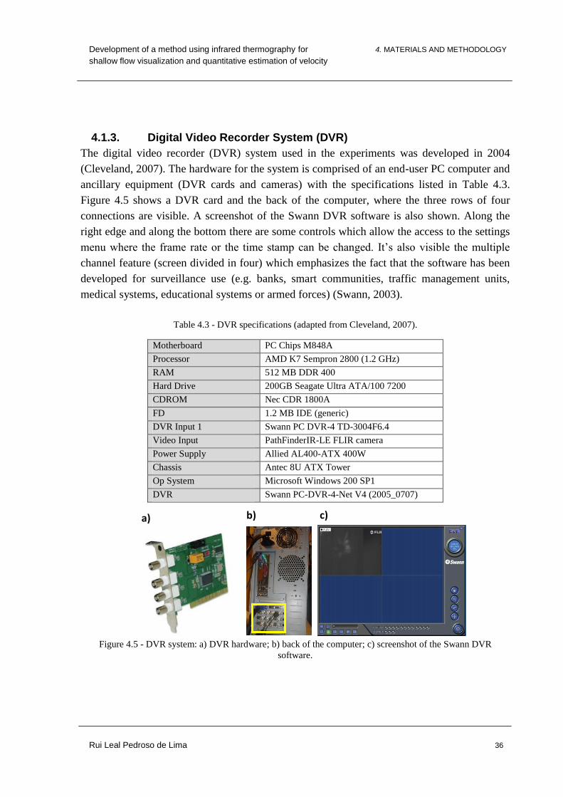
4.1.3. Digital Video Recorder System (DVR) ......................................................................... 36

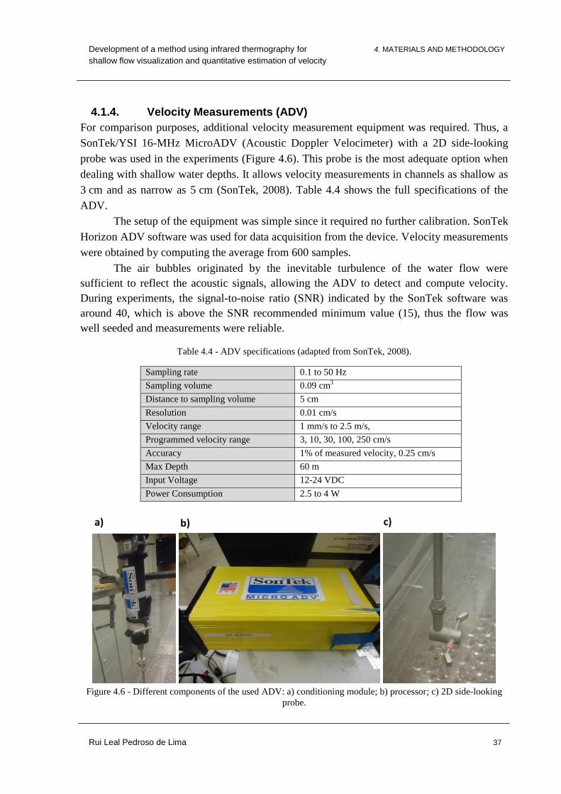
4.1.4. Velocity Measurements (ADV)..................................................................................... 37

4.2. Procedures ............................................................................................................................. 38

4.3. Images Interpretation............................................................................................................. 39

4.4. Heat Generation..................................................................................................................... 42

4.4.1. Hot Water Addition ....................................................................................................... 43

4.4.2. Heated Metal Slab ......................................................................................................... 44

4.4.3. Heat Gun ....................................................................................................................... 44

4.4.4. Heated Electrical Wire .................................................................................................. 45

5. RESULTS AND DISCUSSION .................................................................................... 46

5.1. Initial Considerations ............................................................................................................ 46

5.2. Proof of Principle .................................................................................................................. 46

5.2.1. Technique’s Velocity Range. ........................................................................................ 48

5.2.2. Effect of Channel Slope ................................................................................................ 49

5.3. Water Heating Variables ....................................................................................................... 49

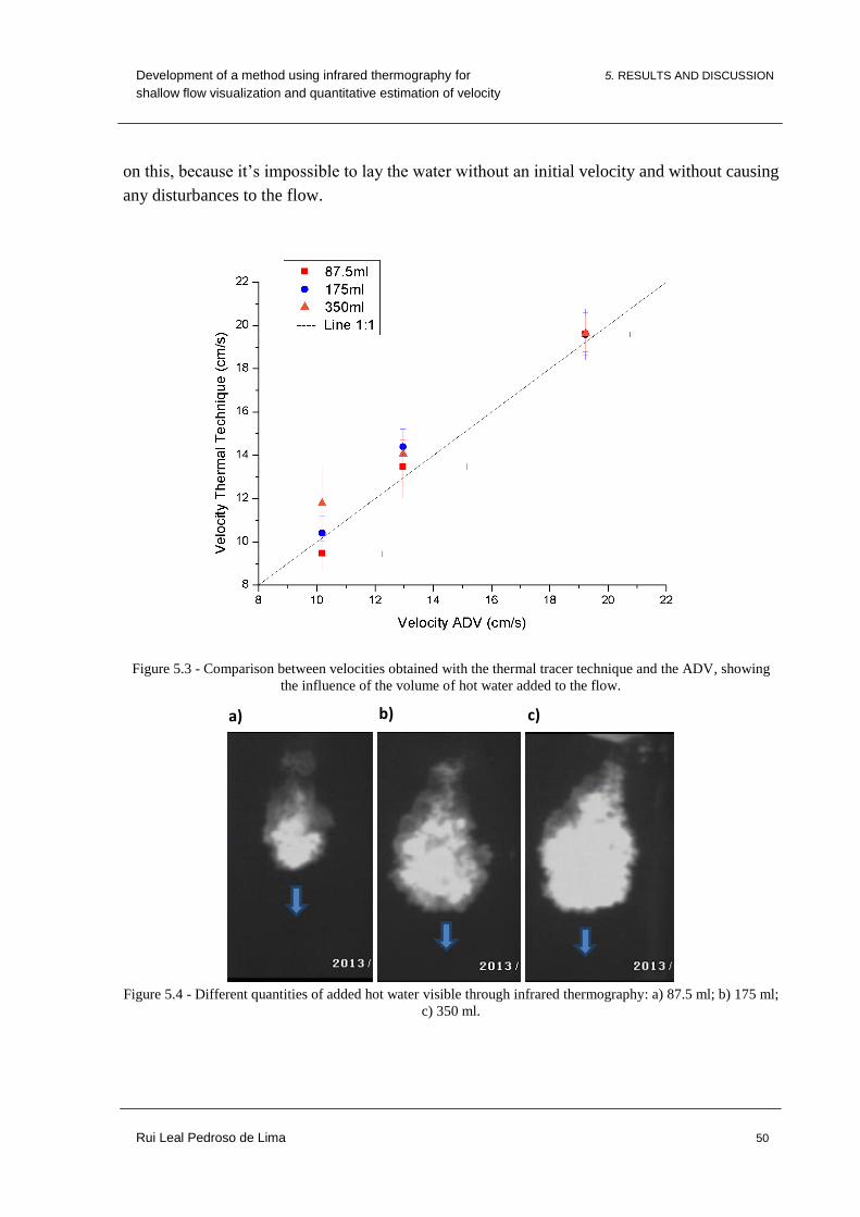
5.3.1. Different Quantities of Added Water ............................................................................ 49

5.3.2. Wider Container ............................................................................................................ 51

5.3.3. Distance from Hot Water Addition Point ...................................................................... 51

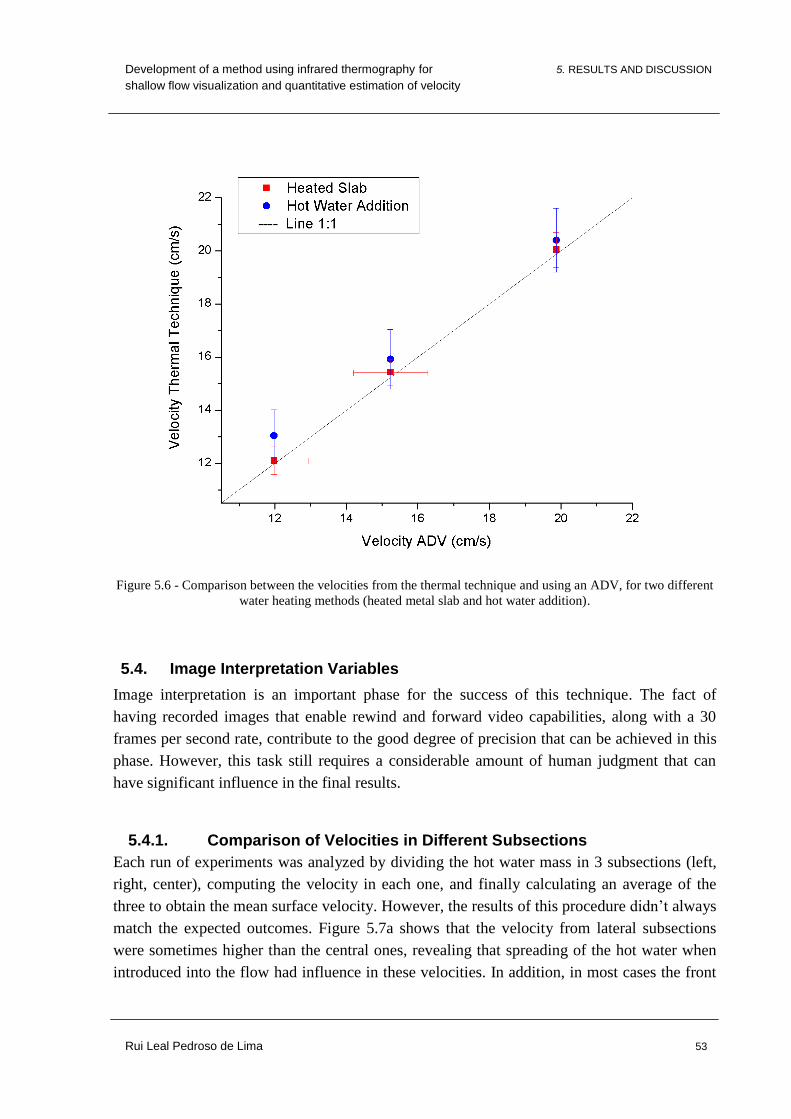
5.3.4. Heated Metal Slab Experiments .................................................................................... 52

5.4. Image Interpretation Variables .............................................................................................. 53

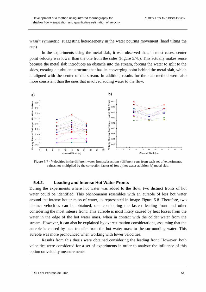
5.4.1. Comparison of Velocities in Different Subsections ...................................................... 53

5.4.2. Leading and Intense Hot Water Fronts .......................................................................... 54



Rui Leal Pedroso de Lima vi

5.5. Additional Experiments ......................................................................................................... 56

5.5.1. Effect of Vegetation ...................................................................................................... 56

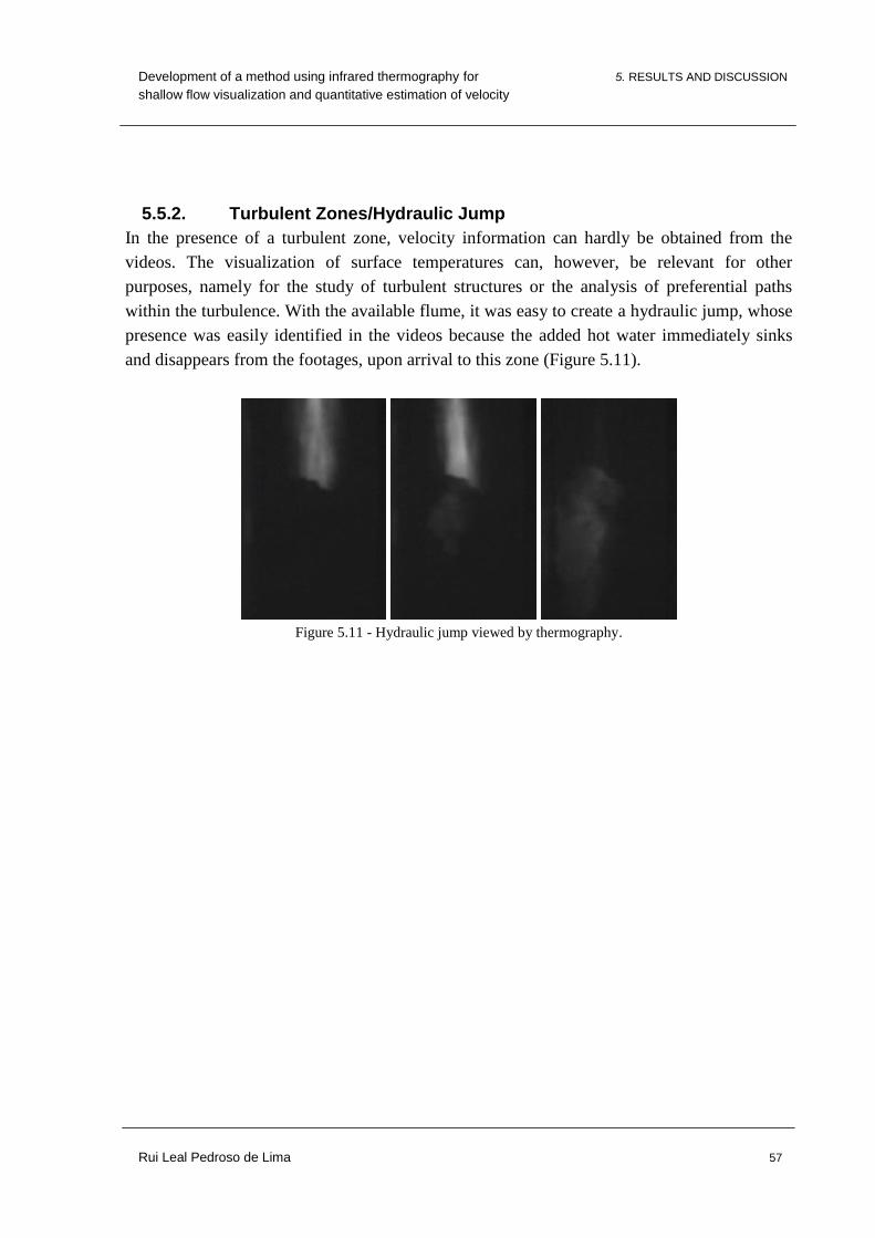
5.5.2. Turbulent Zones/Hydraulic Jump .................................................................................. 57

6. CONCLUSIONS ........................................................................................................... 58

REFERENCES ......................................................................................................................... 61

Development of a method using infrared thermography for LIST OF FIGURES


Rui Leal Pedroso de Lima vii

LIST OF FIGURES

Figure 1.1 - Idealized moving hot water mass. ............................................................................. 2

Figure 2.1 - Example of hydraulic structures for flow measurements: a) sharp crested weir

(Geocashing, 2013); b) flume (Clearfield County, 2013). .................................................. 9

Figure 2.2 - Velocity variations in the cross section (Rantz, 1982): a) typical vertical

velocity profile obtained by an ADCP; b) schematic of the velocity variation in the

cross section. ..................................................................................................................... 10

Figure 2.3 - Example of current meters: a) pygmy-price (Gurley Precision Instruments); b)

propeller type (Hydro-Bios; c) propeller type (Scottech). ................................................ 13

Figure 2.4 - Electromagnetic measurements: a) large scale electromagnetic river gauge

(Newman, 1982); b) current meter (Quantum Dynamics). ............................................... 15

Figure 2.5 - a) ADCP (Teledyne RD Instruments); b) ADCP attached to a boat (Coz,

2008); c) ADCP remotely controlled boat (Coz, 2008). ................................................... 17

Figure 2.6 – a) ADV probe details; b), Sontek ADV device (Conditioning module, probe

and processor). .................................................................................................................. 17

Figure 2.7 - Float measurements: a) procedure illustration (Sanders., 1998); b) different

types of floats (Boiten, 2000). ........................................................................................... 19

Figure 2.8 - Dye tracing field experiments examples: a) Rhodamine (Global Underwater

Explorers, 2013); b) Fluorescent dyes (Fondriest, 2013) .................................................. 22

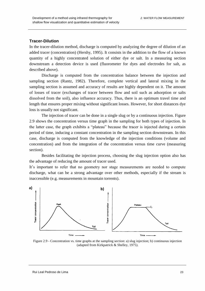
Figure 2.9 - Concentration vs. time graphs at the sampling section: a) slug injection; b)

continuous injection (adapted from Kirkpatrick & Shelley, 1975). .................................. 23

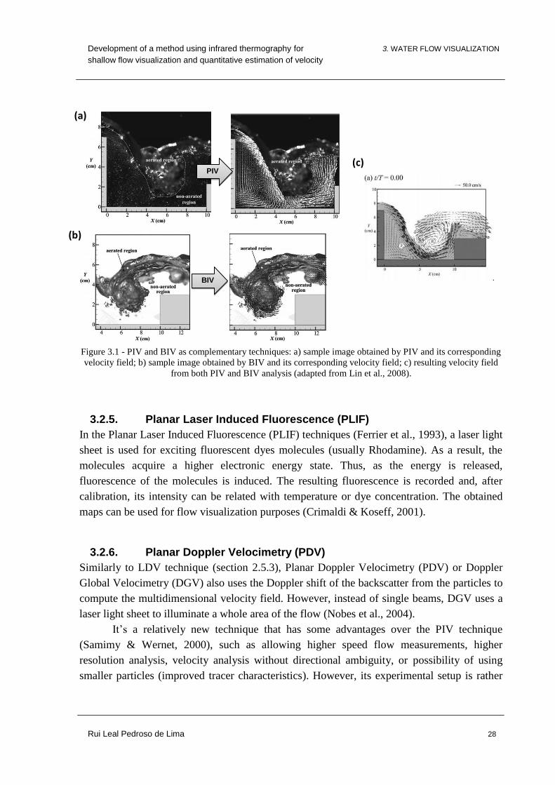
Figure 3.1 - PIV and BIV as complementary techniques: a) sample image obtained by PIV

and its corresponding velocity field; b) sample image obtained by BIV and its

corresponding velocity field; c) resulting velocity field from both PIV and BIV

analysis (adapted from Lin et al., 2008). ........................................................................... 28

Figure 3.2 – a) Sheet to ensure uniform illumination; b) Distribution of the time-mean

concentration, evaluated with the PCA (Rummel et al., 2002). ........................................ 29

Figure 3.3 - Infrared radiation in the electromagnetic spectrum (adapted from MVIM,

2013). ................................................................................................................................ 30

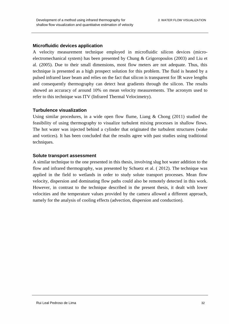
Figure 4.1 - Schematization of the experimental setup. .............................................................. 33



Rui Leal Pedroso de Lima viii

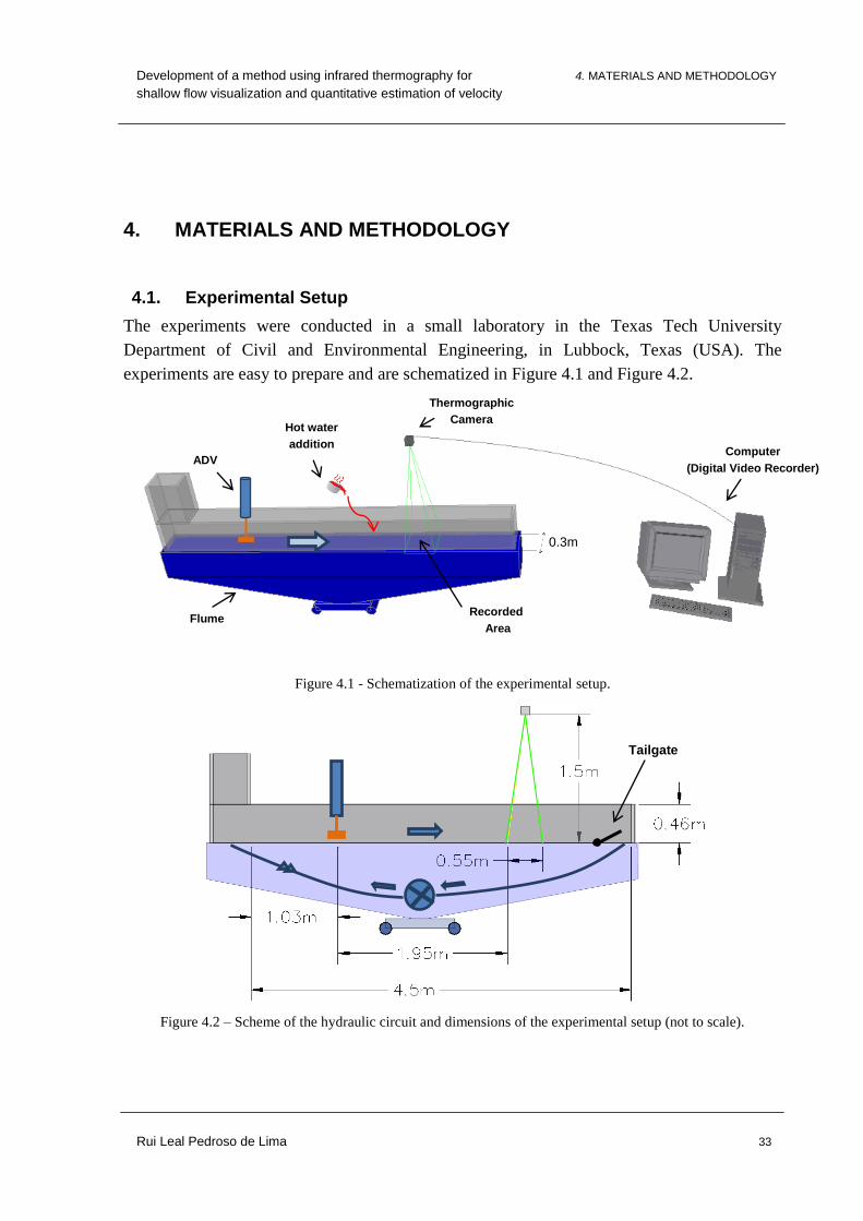
Figure 4.2 – Scheme of the hydraulic circuit and dimensions of the experimental setup (not

to scale). ............................................................................................................................ 33

Figure 4.3 - Flume and details of the flume controls (slope and pump controls, valve

controls and tailgate). ........................................................................................................ 34

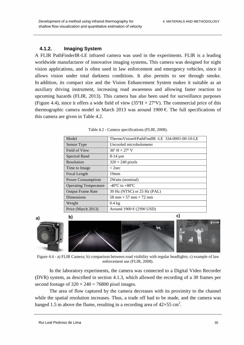
Figure 4.4 - a) FLIR Camera; b) comparison between road visibility with regular

headlights; c) example of law enforcement use (FLIR, 2008). ......................................... 35

Figure 4.5 - DVR system: a) DVR hardware; b) back of the computer; c) screenshot of the

Swann DVR software. ...................................................................................................... 36

Figure 4.6 - Different components of the used ADV: a) conditioning module; b) processor;

c) 2D side-looking probe. ................................................................................................. 37

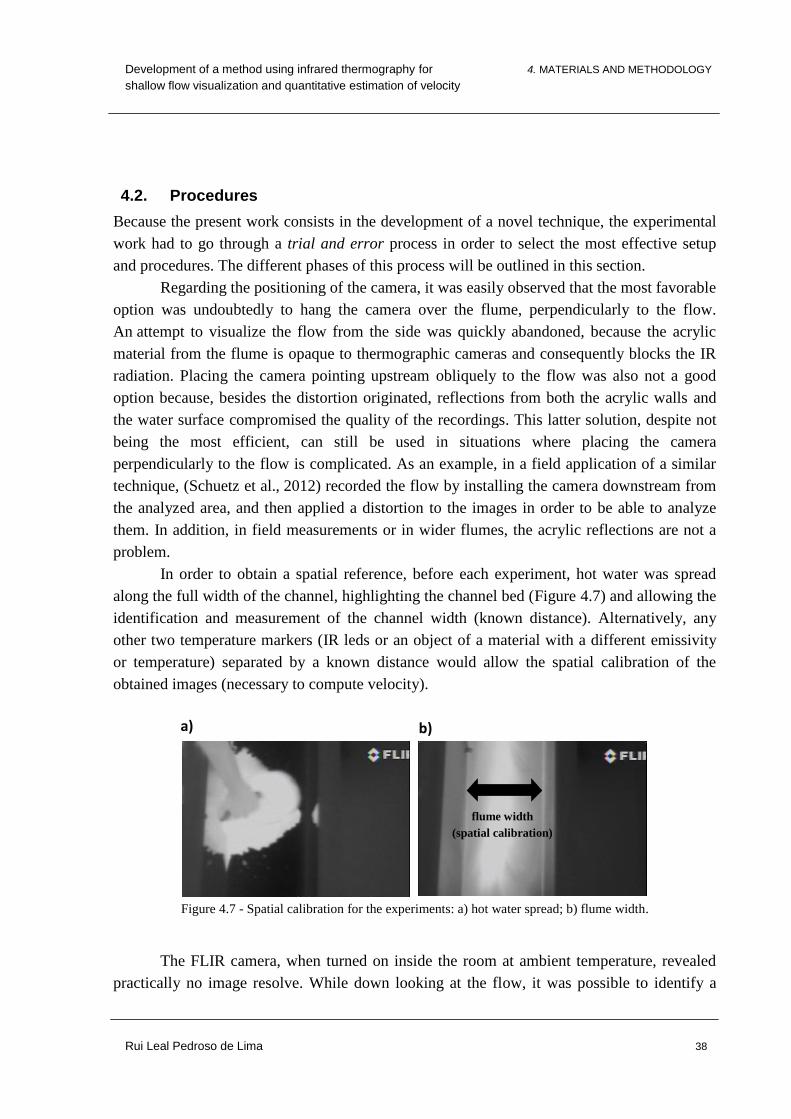
Figure 4.7 - Spatial calibration for the experiments: a) hot water spread; b) flume width. ......... 38

Figure 4.8 – Example of the obtained images and schematization of the procedure used in

the experiments for adding the thermal tracer (hot water) to the flow. ............................. 39

Figure 4.9 - Example of a similar image processing procedure: a) background image; b)

captured heated water c) image with subtracted background; d) final image with

Gauss Low Pass effect (adapted from Chung & Grigoropoulos, 2003)............................ 41

Figure 4.10 - Kinovea software screenshot with the grid and a drawn hot water mass front. .... 41

Figure 4.11 - Image interpretation procedure using Kinovea software. ...................................... 42

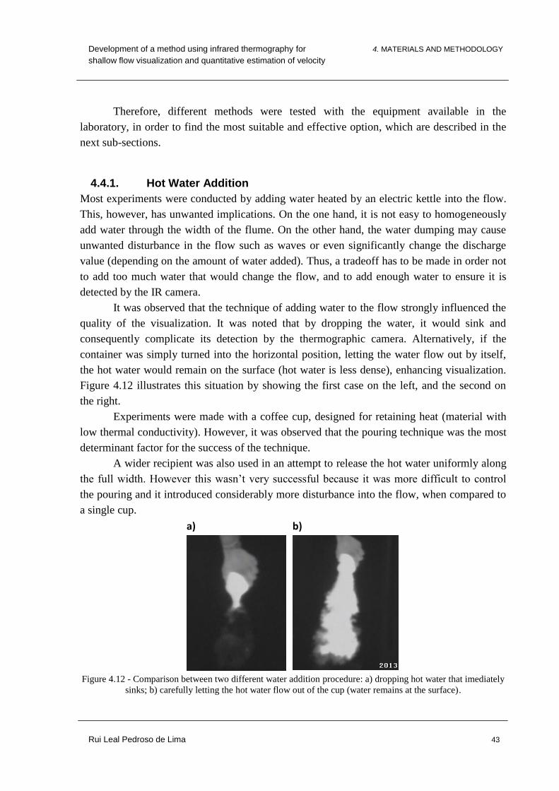
Figure 4.12 - Comparison between two different water addition procedure: a) dropping hot

water that imediately sinks; b) carefully letting the hot water flow out of the cup

(water remains at the surface). .......................................................................................... 43

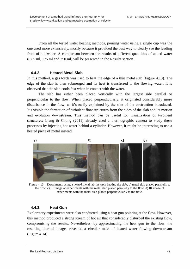
Figure 4.13 – Experiments using a heated metal lab: a) torch heating the slab; b) metal slab

placed parallelly to the flow; c) IR image of experiments with the metal slab placed

parallelly to the flow; d) IR image of experiments with the metal slab placed

perpendicularly to the flow. .............................................................................................. 44

Figure 4.14 - Experiments using a Heat gun: a) Heatgun pointing at the flow; b) IR image

few tenths of second after heating the water; c) heated mass from b) further

downstream. ...................................................................................................................... 45

Figure 4.15 - Experiments using electrical current to heat the flow: a) structure adapted and

placed into the flume; b) an electric wire was connected to a pulsed battery charger;

c) IR image of the heated electric wire and its effect in the flowing water. ..................... 45

Figure 5.1 - Comparison between the velocities obtained using the thermal technique and

the values obtained using an ADV, for different flow velocities, depths and slopes. ....... 47

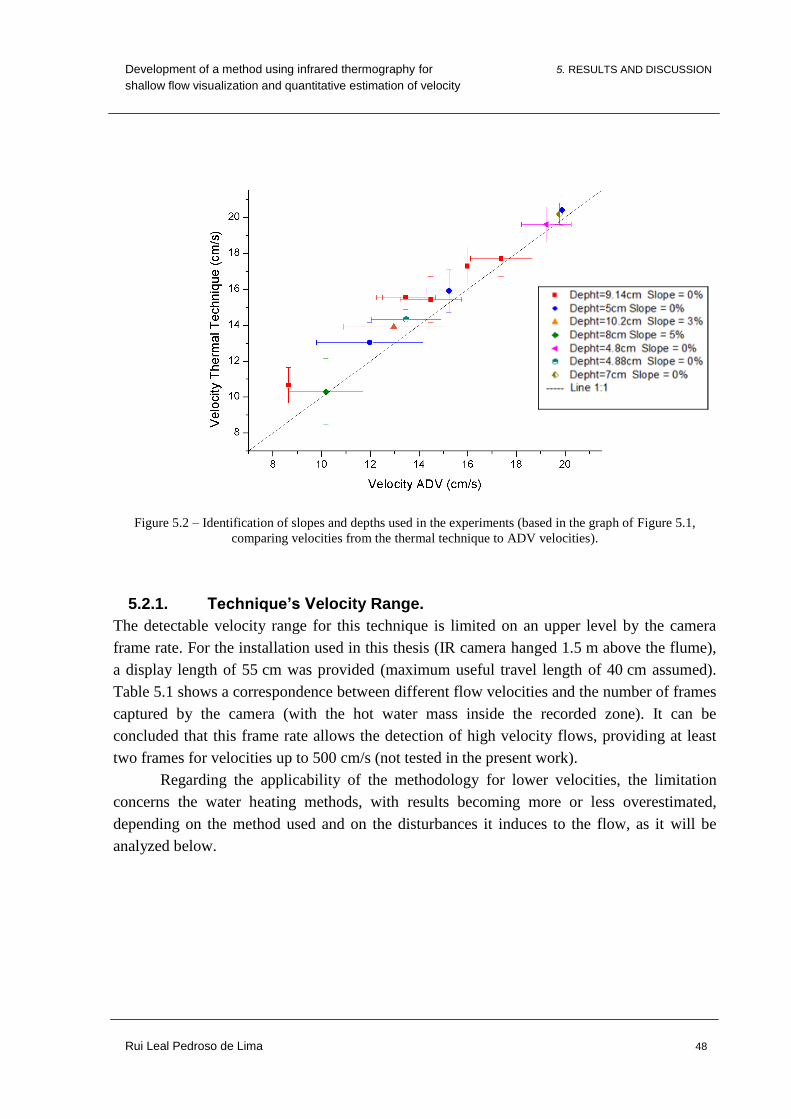
Figure 5.2 – Identification of slopes and depths used in the experiments (based in the graph

of Figure 5.1, comparing velocities from the thermal technique to ADV velocities). ...... 48



Rui Leal Pedroso de Lima ix

Figure 5.3 - Comparison between velocities obtained with the thermal tracer technique and

the ADV, showing the influence of the volume of hot water added to the flow. .............. 50

Figure 5.4 - Different quantities of added hot water visible through infrared thermography:

a) 87.5 ml; b) 175 ml; c) 350 ml. ...................................................................................... 50

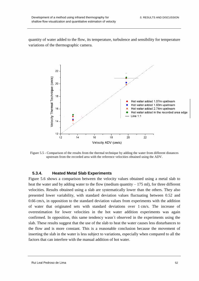
Figure 5.5 - Comparison of the results from the thermal technique by adding the water from

different distances upstream from the recorded area with the reference velocities

obtained using the ADV. ................................................................................................... 52

Figure 5.6 - Comparison between the velocities from the thermal technique and using an

ADV, for two different water heating methods (heated metal slab and hot water

addition). ........................................................................................................................... 53

Figure 5.7 - Velocities in the different water front subsections (different runs from each set

of experiments, values not multiplied by the correction factor α) for: a) hot water

addition; b) metal slab. ...................................................................................................... 54

Figure 5.8 - Illustration of the leading and intense hot water front and its movement

downstream. ...................................................................................................................... 55

Figure 5.9 – Parameters for initial added hot water velocity estimation: cup diameter,

estimated water height during pouring and cross sectional wetted area. .......................... 56

Figure 5.10 - Comparison between velocity of the leading and intense hot water fronts.

Evolution of velocity in the recorded area (three downstream subsections of

0.15 cm), for three different flow velocities. HWAP means hot water addition point. .... 56

Figure 5.11 - Hydraulic jump viewed by thermography. ............................................................ 57

Development of a method using infrared thermography for LIST OF TABLES


Rui Leal Pedroso de Lima x

LIST OF TABLES

Table 4.1 - Flume specifications. ................................................................................................ 34

Table 4.2 - Camera specifications (FLIR, 2008). ........................................................................ 35

Table 4.3 - DVR specifications (adapted from Cleveland, 2007). .............................................. 36

Table 4.4 - ADV specifications (adapted from SonTek, 2008). .................................................. 37

Table 5.1 - Correspondence between flow velocity and number of frames available of the

thermographic images. ...................................................................................................... 49

Development of a method using infrared thermography for ACRONYMS


Rui Leal Pedroso de Lima xi

ACRONYMS

ADCP –Acoustic Doppler Current Profiler

ADV – Acoustic Doppler Velocimetry

BIV – Bubble Image Velocimetry

CCD - Charge-Coupled Device [Camera]

DGV - Doppler Global Velocimetry

DVR – Digital Video Recorder

FPS – Frames Per Second

HWAP – Hot Water Addition Point

IR – Infrared

ITV - Infrared Thermal Velocimetry

LDA – Laser Doppler Anemometry

LDV – Laser Doppler Velocimetry

LIF- Laser Induced Fluorescence

PCA – Planar Concentration Analysis

PDV – Planar Doppler Velocimetry

PIV – Particle Image Velocimetry

PLIF - Planar Laser-Induced fluorescence

PTV –Particle Tracking Velocimetry

Development of an infrared strobe method for shallow flow 1. INTRODUCTION

visualization and quantitative estimation of velocity fields

Rui Leal Pedroso de Lima 1

1. INTRODUCTION AND OBJECTIVES

1.1. Framework and Motivation

Accurate flow measurements devices and techniques are crucial for the success of most

activities related to hydraulics and water resources management. Over the last 30 years,

significant improvements and developments were accomplished, not only resulting in higher

accuracy and quality of the obtained data, but also with the emergence of powerful new

techniques with new capabilities and characteristics, benefiting from the great development of

technology in other areas of knowledge.

The knowledge of velocity profiles are of engineering interest, thus worth of research

focus. Velocity, and consequently discharge (e.g. velocity-area method), is inherently difficult

to measure. Not only the velocity varies in time, varies in depth and it also varies along the

width. In addition, measurement instruments have to deal with problems such as variability of

bed conditions, presence of sediments, accretion and erosion problems, tidal effects,

confluence of water masses, or even the presence of vegetation or air-entrainment. All of

these factors contribute for inaccurate measurements and complicate this important task of

quantifying the flow and obtaining these velocity profiles and fields.

There are however plenty of options for velocity measurement. Most of the principles

used for pressurized flow measurements can also be applied for open channel flows, naturally

with the proper adaptions to face the added complexity originated, for example, by stage or

cross-sectional area variations. However, although these methods are accurate for

measurements under certain conditions, they all have significant limitations. As an example,

most instruments can’t operate at shallow depths.

Shallow flows, as part of the hydrological cycle, often appear in many natural and

urbanized catchments. Also, with the increasing demands on water resources, shallow flows

have gained additional importance. For example, shallow flows are the basis for the design of

rainwater harvesting from parking lots or rooftops. The knowledge of shallow flow behavior

is of engineering interest, due to its implications in water quality, water reserves

characterization and importance for low-slope hydrology. However, the characterization and

quantification of this kind of flows is not easy to achieve, due to its low depths and inevitable

conflict with minimum working depth of measuring instruments that result in considerable

uncertainty.

Identically, research works have also been focusing on flow visualization techniques,

thus new and powerful techniques are emerging, and the existing ones are being improved and

used for different applications. These techniques allow obtaining both qualitative and




quantitative information that can be useful to study various processes and situations. Particle

Image Velocimetry (PIV) is an example of these methods, and allows the quantification of

velocity fields.

Within these flow visualization techniques, thermography appears as a relatively new

technique concerning its application in water resources, hydraulics and hydrology. It has

however considerable potential for remote detection of velocity patterns (e.g. oceans) or for

uses in groundwater or karst hydrology, relying in the detection of natural or artificially

induced temperature gradients. The increase in the use of this technology in the last few years

is explained by the decrease in the price of thermographic cameras, and by its increasing

portability that eases its use, especially in the field.

1.2. Principle

The present thesis consists in the description, proof of principle and some initial experiments

of an emerging technique for estimation of flow mean velocity. The technique uses

inexpensive infrared thermography for visualization and quantification of the motion of an

induced heated mass of hot water acting as a thermal tracer.

The resulting footages from the thermographic camera are sequences of greyscale

images (depending on the camera and software used), which are temperature maps where

higher temperatures are usually represented by brighter colors and lower temperatures by

darker colors. Thus, the heated mass of water is clearly visible as a bright mass moving

downstream. By relying on time of travel considerations, the flow velocity can be computed

through Equation (1.1), by relating spatial and temporal information from the recorded

images, as represented in Figure 1.1.

(1.1)

Figure ‎1.1 - Idealized moving hot water mass.

Ideally, the water should be locally heated along the full stream width, while causing

minimum disturbance to the flow as possible, and as homogeneously as possible. Besides

velocity estimation, this technique can also be useful as a flow visualization method. It is




possible to obtain the horizontal velocity profile and turbulent structures can also be

identified.

The similarities of this method with the tracer velocity method are evident. Thus, it

can be viewed as a variation of these methods, usually used with dyes or salt solutions, but

using a heat/thermal tracer instead. Hot water is likely to perform well as a tracer. As hot

water is still water, most of the characteristics remain approximately the same, thus this tracer

similarity with the stream fluid makes it close to an ideal tracer. However, some of these

properties are known to vary with temperature, such as density or viscosity. As can be easily

computed from a temperature-density relation table, water density at 80ºC (ρ = 0.9718 g cm-3

)

is only around 2.7% lower than the density at ambient temperature (for 20ºC,

ρ = 0.9982 g cm-3

). This difference is most likely not significant for this technique purposes

and the hot water will follow the motion of the flow properly. However, hot water will have

tendency to remain by the top layers, what can actually be an advantage, because it will

enhance surface visualization through the thermographic camera, as it will be described later

on this thesis. Nevertheless, Schuetz et al. (2012) in a similar technique applied to wetlands,

added a salt solution to approximate the densities and reduce this difference. In addition, the

absence of tracer particle agglomeration is also an advantage, when compared to other tracers

(e.g. dyes, salts).

The purpose of this thesis is then to present this two dimensional (planar) technique

that can be useful to surpass some of the most common limitations of conventional velocity

measurement methods, namely when dealing with shallow water depths, where most

instrument can´t operate because of their limited operating depths. Other important strengths

are the simplicity of the setup, which requires relatively inexpensive technology and little

calibration, and the fact that no residue is left on the water (heating might have influence, but

only small volumes are involved).

1.3. Objectives

The main objective of the present thesis is to contribute to the development and design of an

innovative technique for mean velocity estimation using inexpensive thermography

technology and to perform exploratory experiments to test the system (proof of principle).

More specific goals include:

Overview of the most common measurement and visualization techniques and

identification of their main limitations.

Contextualization of the technique within these velocity measurement techniques.

Study the feasibility of the technique, by comparison with a well-established velocity

measurement technique.

Initial laboratory experiments to test the technique for different conditions;




Optimization of procedures in order to improve results, namely:

o Comparison of results using different heating methods;

o Image interpretation options.

Definition of a range of applicability.

Identification of future work prospects.

1.4. Thesis Structure

The present thesis is subdivided in the following chapters:

Chapter 1 – Introduction to the scope of the thesis, principle used in the technique,

objectives and structure of the thesis.

Chapter 2 – State of the art about flow measurement, overview of the different types

of available techniques. Identification of their most significant limitations.

Chapter 3 – Overview of techniques on water flow visualization. Introduction to

thermography technology and some of its most relevant applications for hydraulics

and water resources.

Chapter 4 – Presentation of the experimental installation, equipment and materials

used in this work. Description of the methodology and outline of procedures.

Chapter 5 – Presentation and discussion of the results.

Chapter 6 – Conclusions, outcomes and future work.

Development of a method using infrared thermography for 2. WATER FLOW MEASUREMENT



2. WATER FLOW MEASUREMENTS

2.1. Initial Considerations

The measurement of flow (e.g. discharge, velocity, water depth) has always been crucial for

many different domains. With the management of water resources being a hot topic of the

present times, flow measurement must be seen as fundamental for the planning activity. Flow

measurement provides information about the availability of water resources and its variability

in time and space, allowing a more integrated approach that can be used to support water

management. Knowing the amount of water available is the most important starting point for

determining the best uses for it, reducing the losses and negative environmental impacts. The

planning activity should start with a deep characterization of the study zone in order to

identify the problems (diagnosis) and analyze the available alternatives for solving the

problems and defining the impacts of each of these alternatives. All of these phases depend on

the quality of the available data, such as flow discharge, and are valuable inputs for methods

of decision making support.

The multiple demands for water use also require flow measurement to be accurate.

Irrigation systems are the most recurring example in literature for justifying its importance.

Problems like ensuring a proper distribution of the available water to the multiple users or

crops damaged by overwatering are often referred. Also in the water distribution systems,

flow measurement is fundamental, with proper water losses assessment and water billing

being the key point. Many other activities rely on these measurements for its operation such

as hydroelectric power generation or industry. It’s also important to emphasize the

implications it can have in the cost.

Also in flood control, flow measurements are the basis for the prediction of water

levels and storm water runoff monitoring, allowing the implementation of measures to

minimize the impacts of floods.

Design of hydraulic structures such as channels, water storage reservoirs, dams, flood

control structures, can’t be effectively accomplished without quantifying the discharge that

the structure needs to be able to handle.

Finally, with the recent environmental concerns, quality control of water resources has

become a priority, with considerable pollution control efforts being made. For example,

industrial wastewaters are now required to comply with regulations limits, and the polluter-

payer principle is being applied. All these environmental measures depend on measuring the

discharge and analyzing its chemical properties, in order to quantify their pollution indicators.




Besides the importance of knowing discharge, the knowledge of velocity is also vital

for many studies. For example, soil erosion is a function of flow velocity, meaning that it

must be known to allow the calibration of models for its quantification. Similarly, velocity is

also fundamental in pollutant transport and dispersion modeling.

In addition, flow discharge and velocity undoubtedly influence aquatic organism

energy expenditure, food delivery, waste removal, predator avoidance, and disturbance. Thus,

their measurement is important for its analysis and environmental studies (Hart, 1999).

The research process, in order to obtain valid results, needs accurate data to be

analyzed. Flow discharge and velocity fields are examples of crucial data for researching

water related issues. For example, (Biron et al., 2004) emphasize the need for accurate flow

field data (discharge, velocity, boundary conditions) for parameterization, calibration, and

validation of their developed one-, two-, and three-dimensional river models.

All of these aspects contributed to the development of flow measurement techniques

along the years. In the last few years, new techniques are becoming more popular while others

that were massively used in the past are getting obsoletes due to the development of new and

more effective techniques.

2.2. Shallow Flows

Shallow flows are flows where the water depth is significantly smaller than the width (width

to depth ratio is significantly bigger than 1). This type of flow is known for being turbulent

(Uijttewaal et al., 2001).

Shallow flows are quite common and they can be observed in many different

situations such as in lakes, estuaries, stratified water bodies, coastal areas, lowland rivers,

overland flows or urban areas (Jirka & Uijttewaal, 2004). The determination of velocity fields

in shallow flows is crucial for the success of soil erosion, river morphology or contaminant

transport models, since it’s one of their most important input parameters. Velocity in shallow

flows is affected by several factors, including channel slope or roughness.

Computers already have capacity to solve 3D models for this kind of flow

(Vreugdenhil, 1994). For example, commercial fluid dynamics simulation software

(e.g. FLOW-3D, OpenFoam, Fluent) can be used to model three-dimensional flows with free

surfaces and complex channel geometry (Hirt & Richardson, 1999). However, attending to the

fact that the processes in the horizontal plane are clearly dominant, 3D interactions are often

neglected and shallow flows are analyzed through simplified 2D models that still provide

good approximations.

Shallow flows can be difficult to measure using conventional methods, mostly due to

minimum working depths of measuring devices, vegetation interference, sand deposition or

temporal and spatial changes. In the laboratory, volumetric methods (see section 2.4.1) are




widely used, but they are unsuitable for field measurements, where tracer methods (section

2.5.9) are one of the best options for its measurement.

2.3. Techniques for Open Channel Flows

There are plenty of options for discharge and velocity measurements in open channel flows.

Different authors have been grouping them differently (Holman, 2001). In the present thesis,

discharge measurements were separated from velocity measurements, although they are

related. Other grouping options could consider, for example, single or continuous

measurements, accuracy or applicability (field or laboratory).

The selection between the multiple existing measurement instruments and techniques

is made accounting for many variables related to the equipment itself (e.g. cost, installation

process, portability, availability of power source, dimensions, software) or for the goal of the

measurement (e.g. single or continuous measurement required, precision/accuracy needed,

hydraulic conditions). For example, if the objective is to calibrate one specific method, we

might not need an expensive accurate method with continuous record of flow. Also, there are

many constraints and limitations (e.g. depth, accessibility) that will lead to choosing a method

over the others.

To summarize, the determination of discharge and/or velocity is not an easy task. For

each case, the most suitable method should be used, and the user should be aware of its

uncertainties and limitations. The following sub-sections give an overview of the available

techniques, referring its basic principle as well as their main advantages and limitations,

especially when applied to shallow flows.

2.4. Discharge Measurements

There are several ways to measure discharge. Some of the techniques give discharge directly

(e.g. volumetric and gravimetric). However, discharge is often obtained indirectly, by

measuring different components separately (e.g. velocity, stage, and channel geometry).

In control section methods (e.g. weirs, flumes), discharge can be computed from the upstream

stage, while in the Area-Velocity method (section 2.4.4) velocity measurements are used for

the same purpose. In both cases, the use of secondary instruments is required, for the

knowledge of water levels and cross sectional geometry, respectively.

2.4.1. Gravimetric and Volumetric Methods

The principle of both methods is simple: it consists in collecting the entire flow in a reservoir

and compute discharge by dividing the quantity of water collected by the corresponding

period of time.




In the gravimetric method, this can be done by weighting the amount of water

collected during a given time period. Similarly, the volumetric method follows the same

principle, although measurements involve measuring the volume of collected fluid instead.

Due to the nature of the measurements, this option is less accurate than the gravimetric one,

despite not requiring a weighing scale (a reservoir with a known volume is enough), what can

be an advantage in field measurements.

These method have some evident limitations since they can´t identify changes in the

flow rate and it can’t be used for continuous measurements (the computed discharge is an

average flow rate during a given time period). Another significant limitation is that it can only

be used for low discharge values and for narrow stream concentrated flows. It is, however, a

useful technique for small and simple field and laboratory measurements (Grant & Dawson,

1995). With accuracy values that can reach ±0.04%, gravimetric methods are probably the

most reliable option for discharge measurements, and are often used as reference values in

laboratories. (LEHid/LNEC, 2008)

2.4.2. Natural and Artificial Control Sections and Hydraulic Structures

The goal of a control section is to maintain a flow with well-defined characteristics (critical

flow). An ideal control section varies neither in space nor in time. These control sections can

be natural or artificial, as long as they are stable in order for the rating curves (discharge

versus stage graph) to remain valid. When weirs or flumes are built, they induce changes in

water level in the nearby region. Under these critical conditions, discharge can be computed

only from the upstream stage (downstream head has no influence), since there is a unique

water level for each value of discharge. For artificial control sections, the relation between

stage and discharge is well known, so tabulated ratings can be used (Grant & Dawson, 1995).

Flow measurement through this method requires auxiliary methods for stage determination,

often referred as secondary methods.

Weirs are hydraulic structures (Figure 2.1a) where an obstruction to the flow is applied

in order to obligate the water to flow though the opening (notch). Weirs are often classified by

the shape of the notch that can be rectangular, V shaped (V-notch) or trapezoidal (Cipolletti).

Flumes can be described as an artificially shaped channel flow section (Figure 2.1b),

where the area and slope are modified, forcing the flow to acquire critical conditions,

resulting in changes in velocity and stage. This is usually obtained by a contraction of the

section (vertical and horizontal), restricting the flow, followed by expansion to the normal

channel width. The most common flumes are Parshall flumes, ramp flumes and trapezoidal

flumes (Bos, 1985).

Submerged orifices can also be used for flow measurement in open channels. An

orifice is a well-defined, sharp-edged opening in a wall, through which flow occurs.




Discharge can be computed from the variation between upstream and downstream head and

from the characteristics of the orifice. Submerged orifices result in less head loss when

compared to weirs. However, they have more problems with the deposit of sediments and

other objects that may cause obstruction of the orifice. They’re usually installed when the

conditions for building a weir or a flume are not adequate. (USBR & USDA, 2001)

The main limitation of these control section methods is that they require building a structure

which, sometimes, it’s neither possible nor desirable. Besides, unstable bed conditions, ice

and vegetation obstruction may reduce accuracy. Thus, regular maintenance is crucial to

ensure data quality. It is also an intrusive method which changes the conditions of the flow by

placing an obstruction to the flow.

Figure ‎2.1 - Example of hydraulic structures for flow measurements: a) sharp crested weir (Geocashing, 2013);

b) flume (Clearfield County, 2013).

2.4.3. Empirical Formulas (Slope-Area Method - Control Channel)

Flow can also be estimated using empirical formulas and coefficients. For example, the

Gauckler–Manning–Strickler formula can be used to compute discharge or velocity, based on

some parameters such as the cross sectional area of flow, hydraulic radius, average slope, and

the coefficient of roughness. However, this method implies the use of auxiliary methods to

determine the referred parameters (Boiten, 2000).

Manning roughness coefficients have been tabulated for many different conditions and

materials. Its determination has been object of many research studies. Nevertheless, this

coefficient actually involves parameters such as surface friction or wave resistance that

originate uncertainties. Therefore, its determination is difficult for densely vegetated zones,

shallow flows, or in alluvial channels with continuously changing bed forms, whose

complexity of processes complicate this task. Ding et al. (2004) presented a numerical method

based on optimal theories for identifying Manning roughness coefficients in shallow water

flows, that emphasizes the difficulties that can be found when applying this method, under

a) b)

http://www.geocaching.com/seek/cache_details.aspx?guid=df052868-211e-4cc7-a112-665b9c230359

http://www.ettaro.com/subdomains/amd/index.php?option=com_content&view=article&id=8&Itemid=121




these conditions. Furthermore, the application of these formulas can be seen as a control

channel method, which implies the existence of an uniform flow. Therefore, in order to

successfully apply the Manning formula, some hydraulic and geometric conditions must be

fulfilled.

Similarly, other formulas can be used, such as Chézy’s formula that considers mean

velocity as a function of the hydraulic radius, the bottom slope and the Chézy coefficient

(e.g Dalrymple & Benson, 1984; Hershy, 1995).

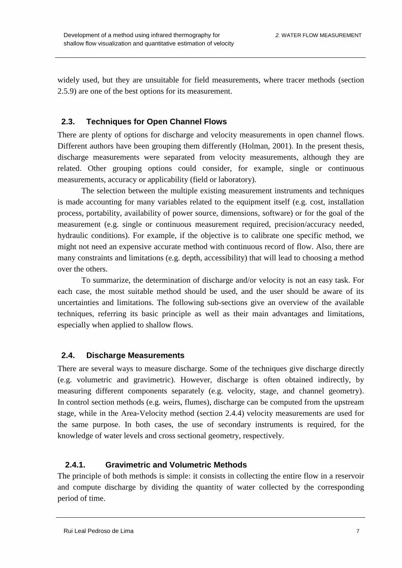
2.4.4. Area-Velocity Method

The Area-Velocity method uses the continuity equation to compute discharge from the

geometry of the cross section and from the mean velocity in this same section. In order to

compute these quantities, the cross section is divided into several subsections

(Ardiclioglu et al., 2010). The geometry is obtained by performing stage measurements in

each one of them (depth at the middle of the subsection). Mean velocity is obtained from

single point velocity measurements at different verticals and depths along the width of the

stream. However, the adoption of a mean velocity to describe the velocity in the cross section

is a considerable simplification. The distribution of the velocity of the cross section is non-

uniform and exhibits considerable variation both through the depth and width, as represented

in Figure 2.2. Vertical profiles have a parabolic distribution of velocity, with the point of

maximum velocity occurring around 10% of total depth below the surface. Horizontally, the

maximum velocity occurs in the center of the channel, decreasing as it approaches the edges.

a) b)

Figure ‎2.2 - Velocity variations in the cross section (Rantz, 1982): a) typical vertical velocity profile obtained by

an ADCP; b) schematic of the velocity variation in the cross section.

In order to properly describe velocity fields, different readings at different depths and

at different verticals along the width of the stream are necessary. Ideally, mean velocity would

http://pubs.usgs.gov/sir/2006/5226/

http://www.jland.org/swat/e41/lab4/




be computed from the integration of velocity profiles. As a simplification, there are several

methods to establish the relationship between these readings and the mean velocity at each

subsection, such as the vertical velocity curve method, the two point method, or the six tenths

depth method (Buchanan & Somers, 1969). These methods may require a variable number of

readings, feature different accuracy, and be more suitable for distinct situations (depth,

vertical variations in water speed, equipment used). These methods are crucial to properly

estimate the mean velocity of the non-uniform vertical velocity field of open channel flow.

The accuracy of the method increases with the number of subsections studied and with

the number of measurements in each vertical. It’s also important to ensure that the main flow

direction is perpendicular to the cross section, thus the selection of the measuring site and

section is important for the success of the method.

Measurements may require various pieces of equipment (e.g. cablecars for

transportation of the operators, unmanned cableways, bridgeboards, cranes for measurements

from bridges) (Hershy, 1995). The need for extra equipment increases the cost of the

measurements and complicates the execution.

2.5. Velocity Measurements

Velocity measurement techniques can measure velocity locally (single direction, or 3D), or

can measure the mean velocity directly. There are also methods that can swipe the full depth

(and width) and obtain the velocity profile (e.g. ADCP or current meters together with a boat).

Finally, some methods allow to measure the velocity continuously, while others can’t

consider the time variable, thus disregarding variations of velocity with time.

2.5.1. Force Displacement

Force displacement methods are based in the principle that the strength of the water against a

mass is proportional to flow velocity.

An example of these methods is a deflection meter, where a vane (vertical or

horizontal axis) is hanged into the flow and its deflection is measured. Vanes can also be used

to directly obtain the discharge (e.g. Larsen, 1992, USBR & USDA, 2001). For this purpose,

vanes have to be calibrated and shaped accordingly to the geometry of the channel. Although

vanes are expensive, they can be used in multiple sites by installing them in permanent pivots

that are usually built to support the removable vanes. Similarly to traditional current meters,

vane deflection meters should not be used if the flow contains considerable amounts of solids

and sediments because it might damage the equipment.

Pendulum type meters are another good example of force displacement methods

(Boiten, 2000). In this case, a submerged mass is hanged by a wire (similar to a pendulum)

and flow velocity can be estimated by measuring the angle of displacement of the wire.




Depending on flow velocities, masses of different shapes and materials are available.

Coefficients may be necessary for corrections for the bending of the wire. This technique is

useful for measurements in shallow rivers or channels.

The effect of wind in the exposed part of both the vane and the wire from the

pendulum can originate significant errors, which can, however, be minimized by installing a

windbreak system.

2.5.2. Velocity Head Rod

This simple and inexpensive technique uses the proportionality between flow velocity and the

upstream height increase (jump) caused by the insertion of a graduated rod in the water

(Boiten, 2000). First, with the sharper edge pointed upstream, the stream depth is measured.

The rod is then placed sideways to the flow, originating an obstacle that causes disturbance

upstream of the rod, namely a jump. By measuring the depth for these new conditions, the

height of the induced jump can be computed and used in tables or abacuses that provide the

corresponding velocity (Carufel, 1980).

This technique is useful for casual measurements in small streams and works well in

the presence of debris or vegetation. It has some limitations, namely the difficulty of detecting

depth variation for slow velocities or in holding the rod against the flow

(Fonstad et al., 2005).

2.5.3. Anemometry

Hot Wire Anemometers

This method’s basic principle consists in relating the fluid velocity to the heat lost when

placing a heated wire in contact with the moving flow. The transfer of heat to the surrounding

fluid can be measured by monitoring the energy needed to maintain a constant temperature in

the wire. Different kind of probes can be used, and they are chosen taking into consideration

many factors, such as the type of flow to be measured, medium (e.g. water, air; widely used

for measuring wind velocities) or the expected velocity range. Some examples of probes are

wires, fiber, films or arrays (Jørgensen, 2002). This technique requires computational analysis

and calibration. Because the sensors are fragile, this technique can’t be used under aggressive

conditions (e.g. presence of debris or sediments).

This technique only provides a measure of the turbulence within the flow. Thus, its

aim is different of the other techniques here presented and it is only here described to

emphasize this difference.




Laser Doppler Velocimetry (LDV)

Laser Doppler Velocimetry (LDV), also known as Laser Doppler Anemometry (LDA) is a

well-established optical method for single point velocity measurements (Drain, 1980).

Similarly to other methods, the flow has to be seeded with particles prior to the experiments.

The method involves the use of two continuous laser beams converging at one point (Albrecht

et al., 2003). When tracer particles pass through that point, they reflect the incident light back

to the optical system. By collecting this scattered reflected light (backscatter) and analyzing

its Doppler shift in wavelength it’s possible to obtain the local 3 different components of

velocity.

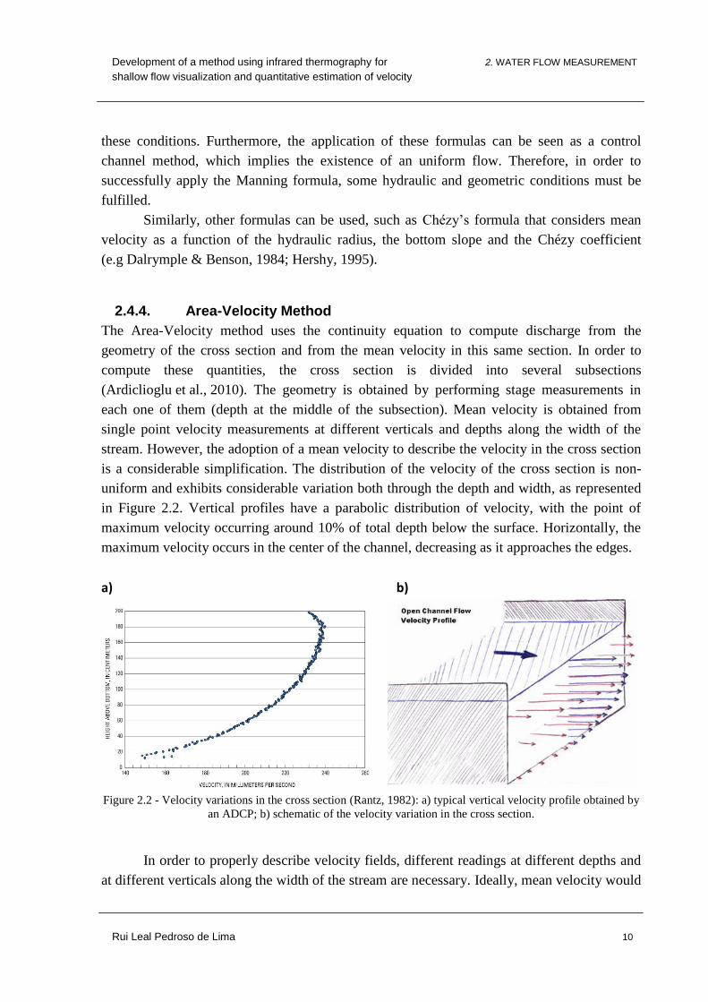
2.5.4. Mechanical Current Meters

Current meters are devices to locally measure the velocity of flow (Figure 2.3). The water

movement induces the rotation of a small rotor that can be installed on a vertical or horizontal

axis. The velocity of the water can be computed from its proportionality with the angular

velocity of the rotor (Boiten, 2000).

The use of current meters has some limitations or drawbacks (Hershy, 1995).

Depending on the depth and width of the channel we intend to measure, the application of this

method may take a long time (pulsating flow requires each single reading to last for at least

40seconds in order to minimize errors. Taking a long time to obtain the readings can be a

problem, especially if rapid changes in stage are expected, jeopardizing the results. Current

meters have also minimum working water depths that can be an important limitation if

shallow flows are to be measured. For this type of flow, pygmy meters are the best option,

with minimum working depths of around 9.14 cm. Besides, current meters don’t work for

flows that are too slow. For example, a pygmy meter needs velocities over 1.83 cm/s in order

to be able to detect it. The presence of debris and sediments also restricts the use of current

meters, since it may damage them.

Figure ‎2.3 - Example of current meters: a) pygmy-price (Gurley Precision Instruments); b) propeller type

(Hydro-Bios; c) propeller type (Scottech).

b) c) a)

http://www.hydrobios.de/en/products/flow-and-current-meters/rod-held-current-meter-rhcm




Another relevant outlook is that current meters must be kept in good conditions, which

require effective maintenance. Without it, the current meter rating (table relating velocity of

the rotor with flow velocity) will most likely provide incorrect values for local velocity.

Many other aspects are susceptible of reducing the instrument accuracy such as the

interference caused by the operator legs while using the current meter or even the influence of

vertical walls proximity. In order to obtain the best possible results, the choice of a good

measuring site is fundamental. It should comply with some criteria, which include the flow

being as rectilinear and regular as possible (flow predominately in a single plane), the use of a

stable cross section. Otherwise, velocity vectors with different directions (e.g. downwards or

sideways) may cause the meters to spin faster and compromise results (Rantz, 1982).

To sum up, the application of this method should be done carefully, because otherwise, its

results may be erroneous.

2.5.5. Electromagnetic

According to electromagnetic induction principle (Faraday), when water flows through a

magnetic field it generates a voltage. The magnitude of this induced voltage can be used to

compute the average velocity of the flow.

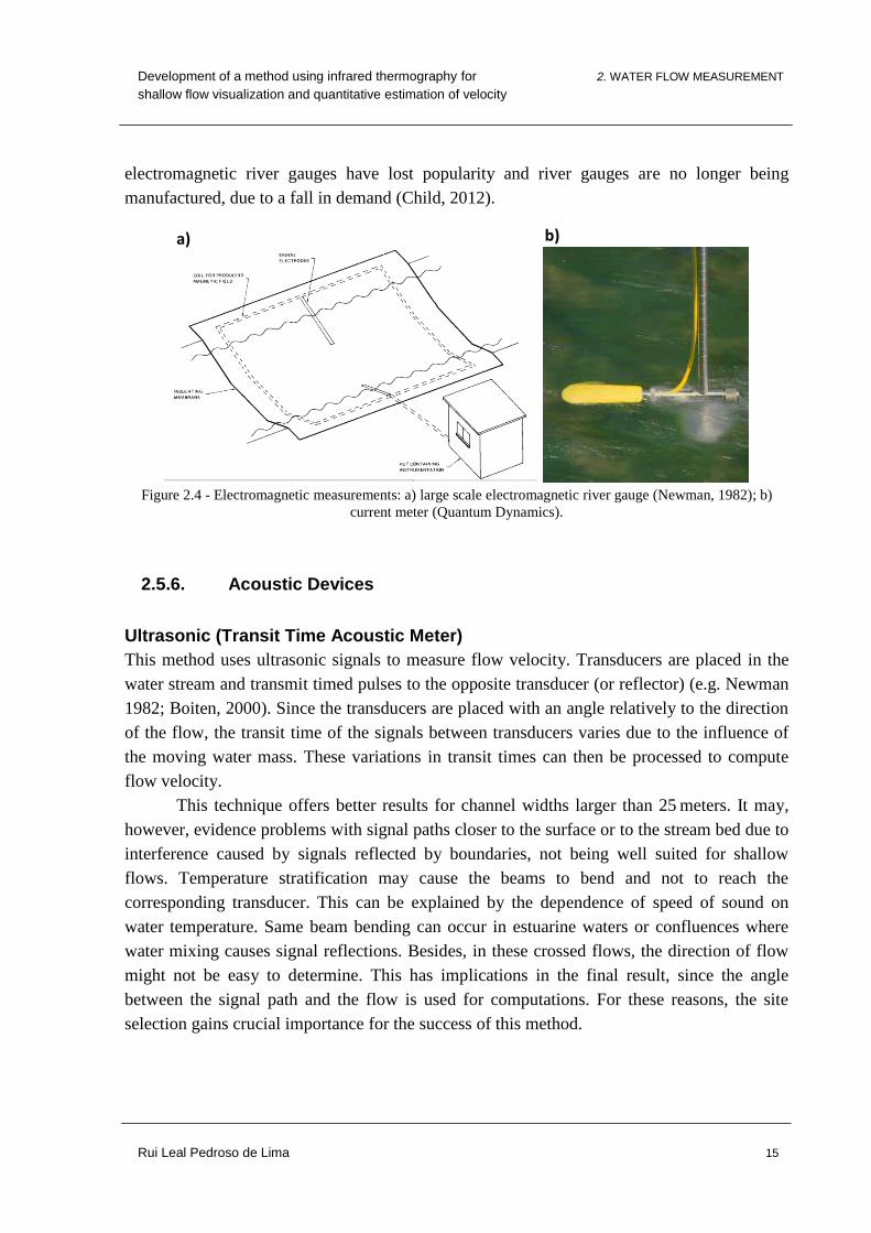
Based in this principle, electromagnetic flow sensors (e.g. Boiten, 2000; Aqua-Data,

2013) comprise a probe equipped with electrodes that sense the voltage induced by the

moving water (Figure 2.4b). These probes have no moving parts and don’t require calibration

(after manufacturer). These devices feature high sensitivity and accuracy, making it a very

versatile instrument that is suitable for measurements in several unfavorable conditions

including shallow or low velocity flows. Although these meters require a minimum

conductivity of the medium (5 μS), this is usually not a problem for uses with water (clean

fresh water conductivity around 50 μS). It is also unaffected by debris or suspended solids in

the flow. Its portability and ease to use are also advantages of this technique.

Newman (1982) developed a large scale application of this electromagnetic method

for measurements in a rivers (Figure 2.4a). In order to create the magnetic field, an

electromagnetic coil is buried under the river bed, and the voltage is picked up by electrodes

in the stream banks. Depending on the bed properties (e.g. conductivity), the induced potential

may be significantly attenuated. To solve this problem, a membrane can be used to isolate the

flow from the river bed, however implying an increase of the cost of the technique (material

and installation). The application range of this method is one of its most important

advantages, since it allows surpassing most common flow measurement limitations: there are

no problems with vegetation, debris content, temperature stratification or variations in stage.

Besides, despite the need to build a permanent installation, the resulting gauging station does

not change the flow conditions (stage) nor becomes a barrier for fish. This method is mainly

used in channels with widths up to 25meters. Despite the usefulness of this technique,




electromagnetic river gauges have lost popularity and river gauges are no longer being

manufactured, due to a fall in demand (Child, 2012).

Figure ‎2.4 - Electromagnetic measurements: a) large scale electromagnetic river gauge (Newman, 1982); b)

current meter (Quantum Dynamics).

2.5.6. Acoustic Devices

Ultrasonic (Transit Time Acoustic Meter)

This method uses ultrasonic signals to measure flow velocity. Transducers are placed in the

water stream and transmit timed pulses to the opposite transducer (or reflector) (e.g. Newman

1982; Boiten, 2000). Since the transducers are placed with an angle relatively to the direction

of the flow, the transit time of the signals between transducers varies due to the influence of

the moving water mass. These variations in transit times can then be processed to compute

flow velocity.

This technique offers better results for channel widths larger than 25 meters. It may,

however, evidence problems with signal paths closer to the surface or to the stream bed due to

interference caused by signals reflected by boundaries, not being well suited for shallow

flows. Temperature stratification may cause the beams to bend and not to reach the

corresponding transducer. This can be explained by the dependence of speed of sound on

water temperature. Same beam bending can occur in estuarine waters or confluences where

water mixing causes signal reflections. Besides, in these crossed flows, the direction of flow

might not be easy to determine. This has implications in the final result, since the angle

between the signal path and the flow is used for computations. For these reasons, the site

selection gains crucial importance for the success of this method.

a) b)




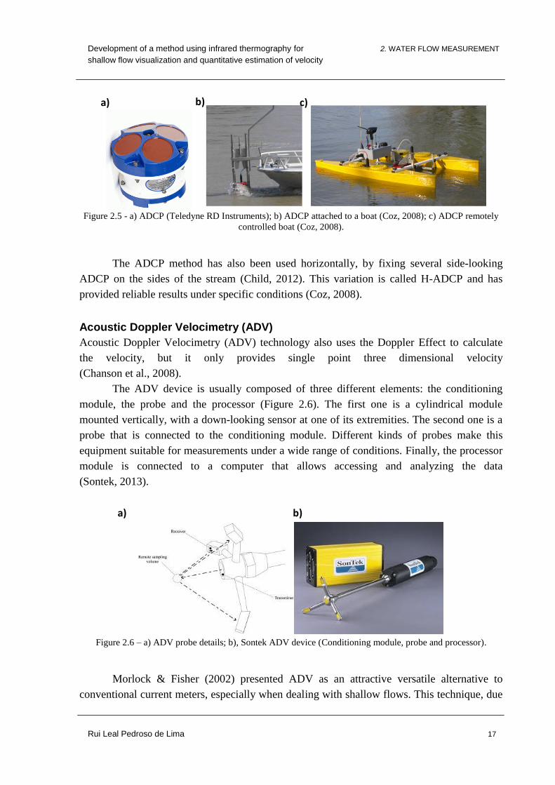
Acoustic Doppler Current Profiler (ADCP)

The Acoustic Doppler Current Profiler (ADCP) technology uses the Doppler Effect to

compute the velocity profile of a stream (Grant & Dawson, 1995). The Doppler Effect

principle states that, as a result of relative motion between the source and the observer, there

is a change in the apparent frequency of the wave. The ADCP device comprises four

transducers (Figure 2.5a) that transmit high frequency sound waves (acoustic pings) that are

reflected by moving particles or air bubbles from the flow. Due to the Doppler Effect, these

reflected waves are collected again by the same ADCP with a different frequency values,

allowing to compute the relative velocity between the moving particles (assumed to be the

same as the flow velocity) and the ADCP equipment (fixed or also in motion). Three of these

transducers are used to compute the velocity in 3 dimensions, while the 4th

transducer is

mainly used for error corrections (Rantz, 1982).

ADCP is a current profiler, meaning that velocity is not measured locally, but a profile

is obtained instead. This data can be used to compute discharge by integrating the velocity

profiles for the full cross section (e.g. area-velocity method). For this purpose, ADCPs are

usually installed in a moving boat in order to swipe the entire cross section of the stream

(Figure 2.5b). The emitted sound signals can be used simultaneously to measure the stage by

time of travel principle. In addition, ADCP devices are also equipped with a pendulum and a

gyroscope that allows them to measure their own speed, in relation to a fixed point in the

stream bed (explains the reduced accuracy of this method when movable beds occur).

However, there are regions of the cross section that can´t be measured. Close to the surface,

there is a region called blanking distance (length for submerging the ADCP device plus the

length transducers need to detect the signals). Near the bottom of the cross section and in

regions close to the shore or vertical walls there is also lot of interference with rebounding

waves (side lobe interference). Because only part of the cross section is measured and to

avoid underestimation of discharge, the missing velocities have to be estimated based on an

idealized velocity distribution, which introduces uncertainty (Rantz, 1982).

In order to detect the reflected sound waves, there must be particles in the water.

However, air bubbles originated by the turbulence of the water flow are usually enough for

this purpose. Because of interference caused by reflections from the boundaries (e.g. surface

and bed), this technique only allows working depths over 0.5m (Forray, 1998).

This method can provide accurate and quick results, which are useful when measuring

rapidly changing flows (e.g. tides), surpassing the traditional time consuming current meters

measurements.




Figure ‎2.5 - a) ADCP (Teledyne RD Instruments); b) ADCP attached to a boat (Coz, 2008); c) ADCP remotely

controlled boat (Coz, 2008).

The ADCP method has also been used horizontally, by fixing several side-looking

ADCP on the sides of the stream (Child, 2012). This variation is called H-ADCP and has

provided reliable results under specific conditions (Coz, 2008).

Acoustic Doppler Velocimetry (ADV)

Acoustic Doppler Velocimetry (ADV) technology also uses the Doppler Effect to calculate

the velocity, but it only provides single point three dimensional velocity

(Chanson et al., 2008).

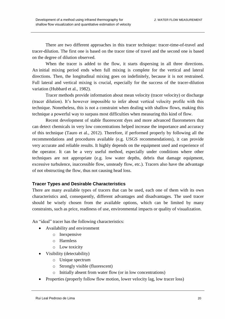
The ADV device is usually composed of three different elements: the conditioning

module, the probe and the processor (Figure 2.6). The first one is a cylindrical module

mounted vertically, with a down-looking sensor at one of its extremities. The second one is a

probe that is connected to the conditioning module. Different kinds of probes make this

equipment suitable for measurements under a wide range of conditions. Finally, the processor

module is connected to a computer that allows accessing and analyzing the data

(Sontek, 2013).

a) b)

Figure ‎2.6 – a) ADV probe details; b), Sontek ADV device (Conditioning module, probe and processor).

Morlock & Fisher (2002) presented ADV as an attractive versatile alternative to

conventional current meters, especially when dealing with shallow flows. This technique, due

a) b) c)

http://wavenet.csir.co.za/MeasuringInstrumentation/adcp.htm

http://portal.tugraz.at/portal/page/portal/TU_Graz/Einrichtungen/Institute/Homepages/i2130/software/ADCPtool




to its similarity with ADCP, shares most of its advantages and disadvantages. However the

main advantages referred are its simple maintenance, no need for frequent calibration, and

high accuracy results.

Both the acoustic Doppler methods (ADCP and ADV) have become important options

for routine measurements, due to its safety, speed of measurements, simpleness of installation

and relatively low cost (Morlock & Fisher, 2002).

2.5.7. Surface Velocity

Radar Instruments

In this method, a radar sends signals and collects its reflections from particles and roughness

of the surface of the stream (Costa et al., 2000). Similarly to the ADCP method (section

2.5.6), software analyzes the shifts in frequency (Doppler Effect) and computes a value for the

surface velocity. The process of obtaining discharge from the superficial velocity resembles

with the optical method described above.

It’s a non-intrusive method, meaning that it surpasses many of the most common

limitations of flow measurement techniques (e.g. debris). Wind might cause interference in

the surface of the flow. This can be corrected by measuring the wind speed, but at some point

it will preclude its use. Nevertheless, it has been proven to be a valid, safe and useful

technique for flow measurement.

Optical

This method measures the surface velocity without submerging the equipment

(e.g. Rantz, 1982; Kirkpatrick & Shelley, 1975). The flow is observed from above from a

stroboscopic device, usually from a bridge, and the motor speed is adjusted in order to obtain

synchronization of the angular velocity of the mirror with the water surface movement. This is

achieved when there is no apparent motion of the water surface, when observed through the

optical meter. The information obtained from the tachometer is then used to estimate the

surface velocity of the flow.

When computing discharge, the area-velocity method is used. The surface velocities

are converted to mean velocities, usually by considering the mean velocity equal to 80% or

85% of the superficial velocity. This procedure is not precise, introducing inevitable

uncertainties to the results.

Optical meters, as many others non-contact methods, can be useful when traditional

current meters are impossible to use, for example during floods, which originates high flow

velocities and considerable quantities of sediments. However, since it computes velocity

based on surface monitoring, it’s highly incompatible with wind.




Several other different kinds of optical methods are available, and will be overviewed

in section 3, dedicated to flow visualization.

2.5.8. Floats/Drift Tracers

The concept of measuring velocity using floats is quite simple (Figure 2.7). It consists in

placing a floating object in the water and measuring the time it takes between two selected

cross sections (Hershy, 1995). The float should acquire a constant velocity before starting the

measurement and a travel time of at least 20 seconds between the two checkpoints is

recommended. Floats of many different sizes and shapes can be used. Oranges are commonly

referred as an example of the versatility of this method and its usefulness for emergencies

when no other method is available. Also bottles, or longer rods and tubes can be used to reach

deeper zones, in order to the velocity of the floats to be closer to the mean velocity of the

flow. For wider streams, multiple floats should be used alongside.

Discharge can be obtained by converting surface velocity into mean velocity, using a

conversion coefficient (e.g. USBR & USDA, 2001; Rantz, 1982). Therefore, because of the

lack of preciseness of this coefficient, along with the probable experimental errors or the

influence of wind (more significant for lower velocities), the obtained values aren´t very

accurate, which makes this method not suitable for routine data collection.

a) b)

Figure ‎2.7 - Float measurements: a) procedure illustration (Sanders., 1998); b) different types of floats (Boiten,

2000).

2.5.9. Tracer Methods

This technique consists in injecting a substance into the water flow, generally referred as

“tracer”, and in measuring its movement. Thus, it’s an indirect method (the tracer movement

is measured, instead of the flow itself) that relies on the assumption that the motion of the

tracer is exactly the same as the movement of the fluid.




There are two different approaches in this tracer technique: tracer-time-of-travel and

tracer-dilution. The first one is based on the tracer time of travel and the second one is based

on the degree of dilution observed.

When the tracer is added to the flow, it starts dispersing in all three directions.

An initial mixing period ends when full mixing is complete for the vertical and lateral

directions. Then, the longitudinal mixing goes on indefinitely, because it is not restrained.

Full lateral and vertical mixing is crucial, especially for the success of the tracer-dilution

variation (Hubbard et al., 1982).

Tracer methods provide information about mean velocity (tracer velocity) or discharge

(tracer dilution). It’s however impossible to infer about vertical velocity profile with this

technique. Nonetheless, this is not a constraint when dealing with shallow flows, making this

technique a powerful way to surpass most difficulties when measuring this kind of flow.

Recent development of stable fluorescent dyes and more advanced fluorometers that

can detect chemicals in very low concentrations helped increase the importance and accuracy

of this technique (Tauro et al., 2012). Therefore, if performed properly by following all the

recommendations and procedures available (e.g. USGS recommendations), it can provide

very accurate and reliable results. It highly depends on the equipment used and experience of

the operator. It can be a very useful method, especially under conditions where other

techniques are not appropriate (e.g. low water depths, debris that damage equipment,

excessive turbulence, inaccessible flow, unsteady flow, etc.). Tracers also have the advantage

of not obstructing the flow, thus not causing head loss.

Tracer Types and Desirable Characteristics

There are many available types of tracers that can be used, each one of them with its own

characteristics and, consequently, different advantages and disadvantages. The used tracer

should be wisely chosen from the available options, which can be limited by many

constraints, such as price, readiness of use, environmental impacts or quality of visualization.

An “ideal” tracer has the following characteristics:

Availability and environment

o Inexpensive

o Harmless

o Low toxicity

Visibility (detectability)

o Unique spectrum

o Strongly visible (fluorescent)

o Initially absent from water flow (or in low concentrations)

Properties (properly follow flow motion, lower velocity lag, low tracer loss)




o Stability - not decomposable (avoid chemical reactions with other elements

that might be present)

Chlorine quenching

Photochemical decay

o Low adsorption and absorption (minimize tracer loss)

o Density similar to water

o High water solubility

o Low agglomeration (compromises assumption of following the flow)

In brief, a tracer should blend perfectly into the flow, accurately replicating its

movement, while allowing proper visualization and quantification, without any limitations to

its applicability (e.g. price, pollution, etc.). Although there are no ideal tracers, this technique

can still be used with quite good results, if the proper tracer for the objective and nature of the

experiment is selected (Mei, 1996).

The quantity of tracer to be used depends on discharge, downstream distance to the

measuring site or expected loss of tracer. There are formulas, especially for long distance

travel time measurements, for determining the quantity of tracer that has to be added to the

flow (Hubbard et al., 1982). There must be a balance between adding enough tracer to allow

proper visualization and, on the contrary, not to add tracer in excess that might change the

flow characteristics.

There are many types of tracers which include electrolyte tracers (e.g. salt solutions),

dye, magnetized tracers or radioactive tracers. The latter one isn’t used very often, due to

complications with the handling of radioactive materials. Several other tracers have been used

and experimented with, often for qualitative and flow visualization purposes (section 3),

instead of directly for flow velocity measurements, such as the hydrogen bubble (section

3.2.2) or the thymol blue technique (section 3.2.3).

Despite sharing the same principle, each tracer has its own characteristics and requires

different equipment and methods for its detection.

Dye tracers can be tracked visually (only in the tracer velocity method) or alternatively

by using a fluorometer, which improves accuracy. There are plenty of options of substances

that can be used as dye tracers. Experiments have been made with different kinds of dyes

including Rhodamine (BA and WT), Fluorescent dyes (Fluorescein) or even regular food dyes

(Amaranth 85, E 123) (Rummel et al., 2002). Fluorescent dyes are becoming more popular,

due to its visibility even in low concentrations (Tauro et al., 2012).

Another option is to use electrolyte tracers (e.g. USBR & USDA, 2001; Shi et al.,

2012; Tingwu et al., 2005). This is often referred to as the salt-velocity method and consists in

the addition of a salt solution to the flow inducing a change in the electrical conductivity

properties of the water. The passage of the tracer is revealed by establishing and monitoring

an electrical current in the sampling section. The electrical current vs. time graphs allows the




detection of a peak that corresponds to the passage of the tracer (salt increases conductivity

and lowers resistivity of the water).

Similarly, time travel of radioactive isotopes or magnetized materials tracers is

measured downstream by using radiation sensing equipment.

Finally, the use of heat tracers, which is the scope of this thesis, can be accomplished,

for example, by the use of thermographic cameras.

Tracer-Velocity

The tracer-velocity principle is similar to the one explained for the floats technique which can

also be referred to as drift tracers. However, instead of a solid object, the tracer used is also a

fluid that participates in the normal fluid processes, getting mixed and transported within the

flow through convective and diffusion phenomena’s (Figure 2.8). Therefore, the procedure is

to measure the time that the tracer takes to travel between two sections. The distance between

both sections is then divided by the measured time, in order to compute velocity.

In most cases, the velocity of the leading edge is measured. This velocity does not

correspond to the mean flow velocity. Instead, it corresponds to the maximum velocity since

the tracer will follow the highest velocity path. Thus, the obtained velocity must be multiplied

by a coefficient to obtain the mean velocity, and this introduces an error in the estimation.

The tracer-velocity method has the advantage of requiring small quantities of tracer,

when compared to tracer-dilution method (continuous injection). This method can also be

used for long distance measurements (sampling section over 50 km downstream from

injection point). In this case, dye losses along the way can be significant, thus more dye is

necessary.

a) b)

Figure ‎2.8 - Dye tracing field experiments examples: a) Rhodamine (Global Underwater Explorers, 2013);

b) Fluorescent dyes (Fondriest, 2013)

http://www.fondriest.com/news/rhodaminedyetracersystem.htm

http://www.globalunderwaterexplorers.org/content/ames-sink-tracer-test




Tracer-Dilution

In the tracer-dilution method, discharge is computed by analyzing the degree of dilution of an

added tracer (concentration) (Hershy, 1995). It consists in the addition to the flow of a known

quantity of a highly concentrated solution of either dye or salt. In a measuring section

downstream a detection device is used (fluorometer for dyes and electrodes for salt, as

described above).

Discharge is computed from the concentration balance between the injection and

sampling section (Rantz, 1982). Therefore, complete vertical and lateral mixing in the

sampling section is assumed and accuracy of results are highly dependent on it. The amount

of losses of tracer (exchanges of tracer between flow and soil such as adsorption or salts

dissolved from the soil), also influence accuracy. Thus, there is an optimum travel time and

length that ensures proper mixing without significant losses. However, for short distances dye

loss is usually not significant.

The injection of tracer can be done in a single slug or by a continuous injection. Figure

2.9 shows the concentration versus time graph in the sampling for both types of injection. In

the latter case, the graph exhibits a “plateau” because the tracer is injected during a certain

period of time, inducing a constant concentration in the sampling section downstream. In this

case, discharge is computed from the knowledge of the injection conditions (volume and

concentration) and from the integration of the concentration versus time curve (measuring

section).

Besides facilitating the injection process, choosing the slug injection option also has

the advantage of reducing the amount of tracer used.

It’s important to refer that no geometry nor stage measurements are needed to compute

discharge, what can be a strong advantage over other methods, especially if the stream is

inaccessible (e.g. measurements in mountain torrents).

Figure ‎2.9 - Concentration vs. time graphs at the sampling section: a) slug injection; b) continuous injection

(adapted from Kirkpatrick & Shelley, 1975).

a) b)




Correction Factor (α) from Surface to Mean Velocity (Tracers)

When tracers are used for quantitative estimation of mean flow velocity of the flow by

measuring the time of travel of the leading edge, what’s truly being measured it’s the surface

velocity. In order to obtain the mean velocity value, this value must be multiplied by a

correction coefficient, usually referred to by the Greek letter α (Li et al., 1996). However, due

to the intrinsic relation between flow velocity and many other variables and conditions such

as turbulence (defined by the Reynolds number), slope, flow variation with time (steady or

unsteady) or sediment content, the determination and systematization of this calibration

coefficient is still a challenge for researchers. Added complications appear in field

applications of tracer techniques, with even more unknown variables and presence of rocks

and vegetation.

Across literature, different authors presented results obtained for a wide range of

conditions. Some discovered relations with sediment transport, others variation with slope or

even with the Reynolds number (e.g. Zhang et al., 2010; Dunkerley, 2001). Mean correction

factor values fluctuate between 0.53 and 0.67. This illustrates the difficulties, dispersion of

results and even contradictions faced by many researchers that, in the last three decades,

struggled to define this coefficient. In the present thesis, the value proposed by Li &

Abrahams (1996), α = 0.67, will be used, as it’s the commonly recommended value.

2.6. Final Comment on Hydrometry

A wide range of powerful and accurate techniques is now available. The main challenges for

hydrometry (Coz, 2008) are now to maintain and improve data quality, without increasing the

need for more resources (e.g. cost, human resources) for its collection. Standards and goals

should however be achievable and realistic. In addition, environmental concerns have also

become an important topic, (e.g. the use of dyes can be have a negative environmental

impact).

The knowledge of the multiple available techniques and the awareness of their

limitations, applicability and inevitable uncertainties is crucial for the selection of the most

adequate technique and measuring site. The use of various techniques simultaneously (as

complement or to fill each other’s limitations) and the repetition of the measurement process

(if possible, accordingly to the quickness of the technique) are important in order to minimize

potential errors and uncertainties.

Development of a method using infrared thermography for 3. WATER FLOW VISUALIZATION



3. WATER FLOW VISUALIZATION


Some of the previously referred methods illustrate the thin frontier between flow

measurement and flow visualization techniques. In fact, by being able to visualize the flow,

it’s possible to infer about velocity fields. With the recent developments in imaging

technology, significant improvements and results have been achieved from the use of

techniques such as the Particle Imaging Velocimetry (PIV), Particle Tracking Velocimetry

(PTV) or the Planar Concentration Analysis (PCA). There is, however, still a long way ahead,

since it’s complicated to interpret data involving turbulence, complicated boundaries,

viscosity or shock wave effects.

There are mainly three different approaches on which flow visualization is based

(Merzkirch, 1974). The first one consists in adding a different material to the flowing fluid

and then using the referred optical imaging methods to track its motion. Therefore, the tracer

method for flow visualization previously referred in section 2.5.9 belongs to this category.

It’s considered an indirect method since the results are obtained by measuring the tracer

motion instead. The assumption is that the tracer and fluid motion are exactly the same, which

may not be exactly true, especially in unsteady flows.

Another approach relies in the fact that fluid density is a function of the refraction

index. Thus, optical methods are sensitive to these variations in density and allow to obtain a

visual pattern from which quantitative or qualitative data can be obtained. They are non-

disturbing methods and some examples include shadowgraphy, schlieren or interferometry.

Finally, the last approach consists in exposing part of the flow to energy in the form of

heat or electrical discharge in order to mark them and make them visible through the use of

optical methods (thymol blue, hydrogen bubbles). The method described in the present thesis

is a good example of this kind of approach, since it consists in heating the water and then

using a thermographic camera to track its motion. However, in the case of adding hot water to

the flow, this same technique can be classified as a heat tracer technique. Either way, its

principle is to track the heat downstream.

It’s important to emphasize that the flow patterns obtained with these techniques are

quite difficult to analyze and to model, mostly due to the complex processes that are involved,

even using powerful computers. Flow visualization can, however, provide useful qualitative

and quantitative information about flow properties, such as velocity, frequency or density.

It has many applications, especially for analyzing velocity, waves, mixing processes, vortices,

eddies or wakes.




A noteworthy fact is that these flow visualization methods are widely used, not only in

liquid flows, but also in gases.

In the next paragraphs, the most relevant flow visualization techniques for this thesis

purposes will be overviewed.

3.2. Flow Visualization Techniques

3.2.1. PIV and PTV

In the Particle Image Velocimetry (PIV) and Particle Tracking Velocimetry (PTV)

techniques, a flow homogeneously seeded with particles is illuminated by a sheet of light.

Using an optical system, the positions of the particles at consecutive moments are recorded

and its displacements are analyzed. The result is a planar map with instantaneous velocity

vectors that represent the velocity field of the flow (Figure 3.1).

The main difference between PIV and PTV is the obtained image density. In PTV

method, a single particle can unambiguously be tracked (Bradley et al., 2002). On the

contrary, if the distance between particles is too short, it’s no longer possible to track each

particle individually, and the matching of pairs of particles is determined statistically. Thus, in

the PIV method, a not well defined region emerges, where the displacements of particles are

obtained through a statistical method and a spatial correlation analysis is carried to obtain the

velocity field, based on a continuity equation (number of particles remain the same). Because

the motion of more particles is studied, PIV technique provides more information than the

PTV.

Although it’s not a new technique, its use has increased significantly in the last years

due to the easier access to charge-coupled device (CCD) cameras and more powerful

computers. Thus, it has become a well-established as a non-intrusive technique for flow

measurement and visualization of a whole field (e.g. Nobach & Tropea, 2005, Meinhart et al.,

2000). However, this technique still requires a relatively complex and expensive set up

(require high power lasers), hardly suitable for experiments in the field, due to its limited

portability.

3.2.2. Hydrogen Bubbles

By using an electric current to induce an electrolysis in the water, hydrogen bubbles can be

produced to act as visible tracers. The bubbles created, due to their dimension, adequately

follow the motion of the flow, and are another suitable option for flow visualization. The

bubbles are created around the wire and are swept by the flow, following its motion. The

diameters of the bubbles are similar to the diameter of the wire and are visible by illuminating

the stream. Due to flotation, the bubbles show tendency to ascend. Lu & Smith (1985) first




presented the technique as a suitable method for the determination of the local velocity

behavior and how turbulence properties could be evaluated.

3.2.3. Thymol Blue

Thymol blue is often used as a pH indicator, as it allows establishing a pH range

(e.g. Merzkirch, 1974; Merzkirch, 2007). It can either be red, yellow or blue accordingly to

the pH of the solution it contacts with. Relying on the creation of hydrogen ions induced by

electrolysis to increase the overall solution pH, the thymol blue changes color to blue near the

electric wire. By using electric pulses, a well-defined blue line is clearly visible and allows

visualization of velocity profiles.

3.2.4. Bubble Image Velocimetry (BIV)

The Bubble Image Velocimetry (BIV) is often considered a variation of the PIV technique

(Lin et al., 2008). BIV consist in tracking the liquid-gas interfaces present in the flow (e.g. air

bubbles), instead of solid particles used in the PIV. Concerning the illumination and

obtainment of the images, the Shadowgraph method is used. A light is placed behind the flow

and the shadow of the bubbles are captured and consequently processed with PIV software to

correlate its positions in consecutive images to construct the vectorial velocity field. This

procedure dismisses the use of expensive high power laser system, facilitating its

implementation and use in the laboratories.

This technique aims at the visualization of aerated bubbly flows. For example, as the

bubbly aerated regions of the flow are complex to analyze with the PIV method (problem with

uncontrolled scatter of laser light), BIV has been used as a complementary technique to fill

this flaw (Figure 3.1; Ryu et al., 2005). The density and size of the bubbles have to comply

with seeding requirements in order to ensure that they can be identified and separated for the

analysis.

Hillier et al. (2010) also used similar procedures, however successfully using the

classic hydrogen bubbles principle as a seeding medium.




Figure ‎3.1 - PIV and BIV as complementary techniques: a) sample image obtained by PIV and its corresponding

velocity field; b) sample image obtained by BIV and its corresponding velocity field; c) resulting velocity field

from both PIV and BIV analysis (adapted from Lin et al., 2008).

3.2.5. Planar Laser Induced Fluorescence (PLIF)

In the Planar Laser Induced Fluorescence (PLIF) techniques (Ferrier et al., 1993), a laser light

sheet is used for exciting fluorescent dyes molecules (usually Rhodamine). As a result, the

molecules acquire a higher electronic energy state. Thus, as the energy is released,

fluorescence of the molecules is induced. The resulting fluorescence is recorded and, after

calibration, its intensity can be related with temperature or dye concentration. The obtained

maps can be used for flow visualization purposes (Crimaldi & Koseff, 2001).

3.2.6. Planar Doppler Velocimetry (PDV)

Similarly to LDV technique (section 2.5.3), Planar Doppler Velocimetry (PDV) or Doppler

Global Velocimetry (DGV) also uses the Doppler shift of the backscatter from the particles to

compute the multidimensional velocity field. However, instead of single beams, DGV uses a

laser light sheet to illuminate a whole area of the flow (Nobes et al., 2004).

It’s a relatively new technique that has some advantages over the PIV technique

(Samimy & Wernet, 2000), such as allowing higher speed flow measurements, higher

resolution analysis, velocity analysis without directional ambiguity, or possibility of using

smaller particles (improved tracer characteristics). However, its experimental setup is rather

PIV

BIV

(a)

(b)

(c)




complex, what is considerable limitation for DGV to become an accessible alternative to other

methods.

3.2.7. Planar Concentrartion Analysis (PCA)

Rummel et al. (2002) developed a method for dye tracing analysis, where recorded video

images were used to obtain dye concentration values by statistically analyzing color intensity

(Leandro et al., 2012). MathLab is used to convert pixel intensity to concentration values,

according to a transfer equation algorithm, thus creating a concentration map. The process

involves going through several steps to improve image quality and through proper calibration

of the transfer function. Because this technique is very sensitive to illumination variations, the

experimental set up involves the use of sheets in order to ensure good and homogeneous

uniform illumination of the camera’s field of view, making it only suitable for lab

experiments (Figure 3.2).

This technique, when compared to other flow visualization methods such as the PIV,

requires a simple and affordable set up and can be a valuable option for shallow flows dye

tracing analysis.

¨

Figure ‎3.2 – a) Sheet to ensure uniform illumination; b) Distribution of the time-mean concentration, evaluated

with the PCA (Rummel et al., 2002).

3.3. Infrared Technology

3.3.1. Thermography

Infrared (IR) represents the electromagnetic radiation with wavelengths between 0.74 microns

and 1000 microns. This represents the zone in the electromagnetic spectrum (Figure 3.3)

between the visible light and microwaves and humans can perceive it as heat. Every object

above the absolute zero in temperature scale (−273.15°C) emits infrared and its emittance

increases with temperature.

Thermography is a technique for detection and measurement of the radiated thermal

energy (FLIR, 2013). A special lens is used to collect all the infrared radiation in the camera’s

a) b)




field of view which is converted to digital signals. These signals are then processed to obtain

an image that can be displayed in a monitor, associated to a grey or color scale. After

calibration, thermographic cameras can also provide temperature values, depending on the

used software.

However, not the entire IR spectrum is visible through thermography. Most common

IR cameras can detect radiation in the LWIR band (long-wavelength infrared - 8μm-14μm),

which include most applications at ambient temperatures.

Figure ‎3.3 - Infrared radiation in the electromagnetic spectrum (adapted from MVIM, 2013).

It’s important to note that glass is opaque in the long-wavelength infrared (LWIR)

band, blocking the radiation emitted by the objects behind it. In addition, emissivity is a

physical property of materials that describes the efficiency of how it radiates. Thus, two

materials with different emissivity may appear differently in thermal imaging, despite having

the same temperature. It’s also important to emphasize that thermographic cameras detect the

energy that radiates through the surface, not the temperature of the object itself.

Due to the recent reduction of costs of these cameras along with the increased

portability, thermography application range has increased considerably. It has been used

extensively as night vision technology in military and law enforcement operations (Figure

4.4). It is also becoming a consolidated technique for uses in industry, building inspections

and electrical systems diagnosis, mainly because it’s a safe and accurate method of detecting

problems (Page et al., 1992). It is also becoming an important tool for uses in research in

diverse fields of knowledge, since it provides an effective, fast and accurate method of

monitoring temperature.

Microwaves, Radio UV, X-rays




3.3.2. Applications of Infrared Technology in Hydraulics

Along the decades, infrared technology has been occasionally used in hydraulic studies. Due

to the reason referred in the previous section, its applications in water resources, hydrology

and soil and water preservation have recently been developing significantly.

One of its major focus is large scale aerial thermal scans. These can provide valuable

information for various purposes. For example, by obtaining sequences of high resolution

temperature maps (thermal gradients) from oceanic waters, it’s possible to infer about near

surface velocities, as described by Chen et al. (2008), Chen et al. (2012) and

Veron et al. (2008).

Another effective use is to scan watersheds to search for groundwater inflows (seeps)

and karst hydrogeology formations (e.g. Jester, 2000; Campbell et al., 1996). These are easily

identified because groundwater is released with different temperature than surface waters

(e.g. during winter, groundwater is warmer than surface water, exposed to low atmospheric

temperatures), thus appearing with a different color intensity in infrared images (Danielescu et

al., 2009). In addition, these remote sensing techniques can also provide other types of

relevant hydrological information (e.g. water quality indicators, identification of local

pollution sources, characterization of pollutant movement and dispersion) (Rayne &

Henderson, 2004).

However, the use of infrared thermography for these purposes still has to overcome

some weaknesses such as the influence of interference originated by unwanted emissive

radiation, thermal stratification problems, or thermal boundary layer effects.

The use of IR thermography for quantitative flow measurements hasn’t been

extensively explored yet, and its capabilities have yet to be studied. Some successful

examples can already be found in the literature. Below some examples of research works are

presented, which are relevant for the present technique due to their similarity of procedures or

because they share a similar principle.

Thermal Sensors

Sensors using heat related principles (Ashauer et al., 1998) are frequently used in flow

measurements in conduits. Measurements can be based on heat losses considerations

(e.g. thermal anemometers – section 2.5.3). Instead, using the thermal transfer principle, by

measuring the energy and the resulting temperature increment, it’s possible to compute the

flow discharge (e.g. calorimeters). Finally, some sensors are based on the thermal time of

flight principle, where heat pulses are generated and used to compute velocity. The present

thesis approach to measure velocity is similar; however, it’s implemented on larger spatial

and temporal scales.




Microfluidic devices application

A velocity measurement technique employed in microfluidic silicon devices (micro-

electromechanical system) has been presented by Chung & Grigoropoulos (2003) and Liu et

al. (2005). Due to their small dimensions, most flow meters are not adequate. Thus, this

technique is presented as a high prospect solution for this problem. The fluid is heated by a

pulsed infrared laser beam and relies on the fact that silicon is transparent for IR wave lengths

and consequently thermography can detect heat gradients through the silicon. The results

showed an accuracy of around 10% on mean velocity measurements. The acronym used to

refer to this technique was ITV (Infrared Thermal Velocimetry).

Turbulence visualization

Using similar procedures, in a wide open flow flume, Liang & Chong (2011) studied the

feasibility of using thermography to visualize turbulent mixing processes in shallow flows.

The hot water was injected behind a cylinder that originated the turbulent structures (wake

and vortices). It has been concluded that the results agree with past studies using traditional

techniques.

Solute transport assessment

A similar technique to the one presented in this thesis, involving slug hot water addition to the

flow and infrared thermography, was presented by Schuetz et al. ( 2012). The technique was

applied in the field to wetlands in order to study solute transport processes. Mean flow

velocity, dispersion and dominating flow paths could also be remotely detected in this work.

However, in contrast to the technique described in the present thesis, it dealt with lower

velocities and the temperature values provided by the camera allowed a different approach,

namely for the analysis of cooling effects (advection, dispersion and conduction).

Development of a method using infrared thermography for 4. MATERIALS AND METHODOLOGY



4. MATERIALS AND METHODOLOGY

4.1. Experimental Setup

The experiments were conducted in a small laboratory in the Texas Tech University

Department of Civil and Environmental Engineering, in Lubbock, Texas (USA). The

experiments are easy to prepare and are schematized in Figure 4.1 and Figure 4.2.

Figure ‎4.1 - Schematization of the experimental setup.

Figure ‎4.2 – Scheme of the hydraulic circuit and dimensions of the experimental setup (not to scale).

Thermographic

Camera Hot water

addition Computer

(Digital Video Recorder)

Flume

ADV

Recorded

Area

Tailgate

0.3m




4.1.1. The Flume

For the experiments, a flume designed by Engineering Laboratory Design Inc. was used and

provided a channel 0.3 m wide and 4.5 m long (Eldinc, 2013). It was mainly developed for

working as a multipurpose demonstration channel for support of academic courses. Therefore,

different accessories and devices can be easily installed such as weirs of different shapes,

meters or even conduits.

The flume bed and walls are made of acrylic Plexiglas (leak proof joints and good

impact resistance), thus impermeable, smooth and transparent (Figure 4.3). The slope is easily

adjustable by a motorized jacking system. Similarly, the end of the flume has an adjustable

tilting plate that allows depth control. Upstream, a head tank is available, for inducing

pressurized flow, when the conduit circuit is installed. The flume operates as a self-

recirculating circuit with integrated pumps and is controlled by valves that can be regulated

by the user. The full specifications, adapted from manufacturer website, are presented in

Table 4.1.

Table ‎4.1 - Flume specifications.

Maximum Flow Rate 360 l/s

Slope Range -4% to 12%

Overall dimensions 2.28 m × 0.90 m × 4.95 m

Dry Weight 612 kg

Power 0.56 kW

Figure ‎4.3 - Flume and details of the flume controls (slope and pump controls, valve controls and tailgate).




4.1.2. Imaging System

A FLIR PathFinderIR-LE infrared camera was used in the experiments. FLIR is a leading

worldwide manufacturer of innovative imaging systems. This camera was designed for night

vision applications, and is often used in law enforcement and emergency vehicles, since it

allows vision under total darkness conditions. It also permits to see through smoke.

In addition, its compact size and the Vision Enhancement System makes it suitable as an

auxiliary driving instrument, increasing road awareness and allowing faster reaction to

upcoming hazards (FLIR, 2013). This camera has also been used for surveillance purposes

(Figure 4.4), since it offers a wide field of view (35ºH × 27ºV). The commercial price of this

thermographic camera model in March 2013 was around 1900 €. The full specifications of

this camera are given in Table 4.2.

Table ‎4.2 - Camera specifications (FLIR, 2008).

Model ThermoVision®PathFindIR -LE 334-0001-00-10-LE

Sensor Type Uncooled microbolometer

Field of View 36º H × 27º V

Spectral Band 8-14 µm

Resolution 320 × 240 pixels

Time to Image < 2sec

Focal Length 19mm

Power Consumptiom 2Watts (nominal)

Operating Temperature -40ºC to +80ºC

Output Frame Rate 30 Hz (NTSC) or 25 Hz (PAL)

Dimensions 58 mm × 57 mm × 72 mm

Weight 0.4 kg

Price (March 2013) Around 1900 € (2500 USD)

Figure ‎4.4 - a) FLIR Camera; b) comparison between road visibility with regular headlights; c) example of law

enforcement use (FLIR, 2008).

In the laboratory experiments, the camera was connected to a Digital Video Recorder

(DVR) system, as described in section 4.1.3, which allowed the recording of a 30 frames per

second footage of 320 × 240 = 76800 pixel images.

The area of flow captured by the camera decreases with its proximity to the channel

while the spatial resolution increases. Thus, a trade off had to be made, and the camera was

hanged 1.5 m above the flume, resulting in a recording area of 42×55 cm2.

a) b) c)




4.1.3. Digital Video Recorder System (DVR)

The digital video recorder (DVR) system used in the experiments was developed in 2004

(Cleveland, 2007). The hardware for the system is comprised of an end-user PC computer and

ancillary equipment (DVR cards and cameras) with the specifications listed in Table 4.3.

Figure 4.5 shows a DVR card and the back of the computer, where the three rows of four

connections are visible. A screenshot of the Swann DVR software is also shown. Along the

right edge and along the bottom there are some controls which allow the access to the settings

menu where the frame rate or the time stamp can be changed. It’s also visible the multiple

channel feature (screen divided in four) which emphasizes the fact that the software has been

developed for surveillance use (e.g. banks, smart communities, traffic management units,

medical systems, educational systems or armed forces) (Swann, 2003).

Table ‎4.3 - DVR specifications (adapted from Cleveland, 2007).

Motherboard PC Chips M848A

Processor AMD K7 Sempron 2800 (1.2 GHz)

RAM 512 MB DDR 400

Hard Drive 200GB Seagate Ultra ATA/100 7200

CDROM Nec CDR 1800A

FD 1.2 MB IDE (generic)

DVR Input 1 Swann PC DVR-4 TD-3004F6.4

Video Input PathFinderIR-LE FLIR camera

Power Supply Allied AL400-ATX 400W

Chassis Antec 8U ATX Tower

Op System Microsoft Windows 200 SP1

DVR Swann PC-DVR-4-Net V4 (2005_0707)

Figure ‎4.5 - DVR system: a) DVR hardware; b) back of the computer; c) screenshot of the Swann DVR

software.

a) b) c)




4.1.4. Velocity Measurements (ADV)

For comparison purposes, additional velocity measurement equipment was required. Thus, a

SonTek/YSI 16-MHz MicroADV (Acoustic Doppler Velocimeter) with a 2D side-looking

probe was used in the experiments (Figure 4.6). This probe is the most adequate option when

dealing with shallow water depths. It allows velocity measurements in channels as shallow as

3 cm and as narrow as 5 cm (SonTek, 2008). Table 4.4 shows the full specifications of the

ADV.

The setup of the equipment was simple since it required no further calibration. SonTek

Horizon ADV software was used for data acquisition from the device. Velocity measurements

were obtained by computing the average from 600 samples.

The air bubbles originated by the inevitable turbulence of the water flow were

sufficient to reflect the acoustic signals, allowing the ADV to detect and compute velocity.

During experiments, the signal-to-noise ratio (SNR) indicated by the SonTek software was

around 40, which is above the SNR recommended minimum value (15), thus the flow was

well seeded and measurements were reliable.

Table ‎4.4 - ADV specifications (adapted from SonTek, 2008).

Sampling rate 0.1 to 50 Hz

Sampling volume 0.09 cm3

Distance to sampling volume 5 cm

Resolution 0.01 cm/s

Velocity range 1 mm/s to 2.5 m/s,

Programmed velocity range 3, 10, 30, 100, 250 cm/s

Accuracy 1% of measured velocity, 0.25 cm/s

Max Depth 60 m

Input Voltage 12-24 VDC

Power Consumption 2.5 to 4 W

Figure ‎4.6 - Different components of the used ADV: a) conditioning module; b) processor; c) 2D side-looking

probe.

a) b) c)




4.2. Procedures

Because the present work consists in the development of a novel technique, the experimental

work had to go through a trial and error process in order to select the most effective setup

and procedures. The different phases of this process will be outlined in this section.

Regarding the positioning of the camera, it was easily observed that the most favorable

option was undoubtedly to hang the camera over the flume, perpendicularly to the flow.

An attempt to visualize the flow from the side was quickly abandoned, because the acrylic

material from the flume is opaque to thermographic cameras and consequently blocks the IR

radiation. Placing the camera pointing upstream obliquely to the flow was also not a good

option because, besides the distortion originated, reflections from both the acrylic walls and

the water surface compromised the quality of the recordings. This latter solution, despite not

being the most efficient, can still be used in situations where placing the camera

perpendicularly to the flow is complicated. As an example, in a field application of a similar

technique, (Schuetz et al., 2012) recorded the flow by installing the camera downstream from

the analyzed area, and then applied a distortion to the images in order to be able to analyze

them. In addition, in field measurements or in wider flumes, the acrylic reflections are not a

problem.

In order to obtain a spatial reference, before each experiment, hot water was spread

along the full width of the channel, highlighting the channel bed (Figure 4.7) and allowing the

identification and measurement of the channel width (known distance). Alternatively, any

other two temperature markers (IR leds or an object of a material with a different emissivity

or temperature) separated by a known distance would allow the spatial calibration of the

obtained images (necessary to compute velocity).

Figure ‎4.7 - Spatial calibration for the experiments: a) hot water spread; b) flume width.

The FLIR camera, when turned on inside the room at ambient temperature, revealed

practically no image resolve. While down looking at the flow, it was possible to identify a

flume width

(spatial calibration)

a) b)




moving mass of heated water. An example of the obtained images is presented in Figure 4.8.

Brighter colors represent higher temperatures while lower temperature surfaces are darker. It

clearly exhibits the downwards movement of the heated water. Due to high flow speeds, the

image faded fast.

At an early stage, by comparing the velocity of the heated water mass with the velocity

obtained through the use of floats, it was possible to confirm that these procedures could

provide an estimation of the flow surface velocity.

Figure ‎4.8 – Example of the obtained images and schematization of the procedure used in the experiments for

adding the thermal tracer (hot water) to the flow.

The obtained surface velocity was multiplied by a correction factor α=0.67 (Abrahams

& Li, 1998), usually used in tracer methods for converting from the surface velocity to the

mean flow velocity (see section 0 2.5.9).

In order to validate the experiments as a proof of principle of the technique, sets of

experiments were conducted simultaneously with an ADV (section 4.1.4), which is

considered a well-established and trustworthy velocity measurement technique.

The next step was to test different water heating methods and to try to improve the

water heating process. The tested methods are described in section 4.4. Similarly, some notes

on the image processing phase are presented in section 4.3.

4.3. Images Interpretation

The image interpretation phase, due to its direct influence on accuracy, is crucial for the

success of this technique. This process has high resemblances with the dye tracing technique,

where the progression (time of travel) of the dye cloud is measured visually. However, for

dyes, these measurements are usually made using stopwatches and human reaction errors are

likely to be significant. In the present technique, this kind of errors is reduced due to the use

Thermographic

Camera

Flow direction

Hot water mass visible

through Thermography

a) b)




of recorded images. The video player capabilities (e.g. start, stop, move forward, rewind)

allow a precise frame by frame analysis that would be impossible to accomplish with human

reaction time uncertainties. Furthermore, it also allows more time and tools to properly infer

about the heated water mass delimitation (identification of the leading front).

For mean flow velocity estimation purposes, there are two options to analyze the

downstream motion of a mass of tracer. Some authors track the center of mass (Kirkpatrick &

Shelley, 1975) while others assume that the leading edge of the tracer mass is the one that

should be studied (Roels, 1984). Similarly, if fluorometers are being used (in dye

experiments), the peak concentration or the first detected concentrations can be used.

By considering the velocity of the leading edge, the mean velocity will most likely be

overestimated, when compared to cases when the center of mass movement is considered.

In an attempt to improve accuracy and minimize the ambiguity and overestimation in mean

velocity determination through dye tracer methods, Abrahams et al. (1986) proposed a

method for obtaining the mean velocity of a stream, considering the variation of the velocity

along the width of the stream. Based on current meters subsections averaged velocity

Abrahams proposed a division of the stream in subsections and an independent determination

of the leading edge velocity for each subsection. The global mean velocity would finally be

computed from an average of all the velocities.

In the present thesis, an adaptation of Abrahams’ method (Abrahams et al., 1986) will

be used. The leading heated water front will be divided in three subsections and the mean

velocity of the leading edge in each one of them will be computed. The mean velocity of the

whole hot water front will then be obtained by computing the average of the three values.

For wider flumes and therefore wider study zone, more subsections can be chosen, in

order to increase accuracy. For the present experimental setup, it was considered that three

subsections were enough to properly represent the advance of the front.

The experiments resulted in footages in a compressed “.avi” file format. This was a

limitation because some programs are only compatible with the un-compressed “.avi” file

(e.g. imageJ). After several tryouts of multiple video and image editing software, the choice

fell on Adobe’s Premiere Pro CS5.5 for applying some effects to the video, in order to

accentuate and improve the visualization of the heat tracer, and then onto Kinovea, an open

source video player, that stepped up as the most agile and easy to use tool for the quantitative

analysis of the files.

Adobe Premiere CS5.5 is a powerful professional video editing software that allows

users to work directly on the timeline (timeline based). It facilitates the mixing of different

videos and features a big collection of effects. It was used for subtracting background, adding

effects such as contrast, brightness, color substitution, color control, with the objective of

enhancing visualization. Depending on the water heating method, there were cases where this

image treatment could be skipped, because the hot water was already clearly visible. There

were also cases where, even after these steps, it was impossible to properly visualize the




videos. A similar approach was made by Chung & Grigoropoulos (2003) and Narayanan et al.

(2003) where the radiative image of the background was subtracted from the full image with

the heated flow, isolating the tracer. Then, the noise was smoothed using a Gaussian low pass

filter effect. The results of this procedure can be seen in Figure 4.9.

Figure ‎4.9 - Example of a similar image processing procedure: a) background image; b) captured heated water

c) image with subtracted background; d) final image with Gauss Low Pass effect (adapted from Chung &

Grigoropoulos, 2003).

Kinovea is an open source software, developed for sport videos analysis. It’s a video

manipulation tool that allows measurement of distances and angles, point marking, side by

side video comparison, tracking of objects, zoom and other useful features. This program was

used to analyze the footage. It allowed the introduction of a grid and provided other useful

tools like lines, and measurement tools, that facilitated the division of the heated mass in

subsections (Figure 4.10).

Figure ‎4.10 - Kinovea software screenshot with the grid and a drawn hot water mass front.

As an alternative, if video editing software is not available, the frames could easily be

extracted from the video file (e.g. “Free Video to JPG Converter”) and analyzed frame by

frame, as a succession of images. Although the extracted frames are easily identified by the

time stamp in the image, this only provides information to the second, meaning that the




frames had to be counted, and the time between frames must be known and used to compute

velocity. Some early experiments were analyzed using this procedure.

The procedure for the acquisition of data for velocity computations is represented in

Figure 4.11. The images were analyzed by defining two sections (yellow lines) separated by a

variable distance (20 cm in this example). Similarly to the floats’ method (section 2.5.8,

Figure 2.7) the time that the leading edge takes to travel between both sections was measured

(t2-t1). This was registered for three different subsections (left, center, right), whose central

lines are represented in Figure 4.11 by three vertical lines. Finally, the velocity is computed

by dividing the travel distance by the time interval, the mean velocity from the three

subsections is calculated and the correction factor is applied (section 2.5.9).

Figure ‎4.11 - Image interpretation procedure using Kinovea software.

4.4. Heat Generation

An ideal water heating method would be able to heat the water to a temperature easily

detected by the camera, while causing low flow disturbance. It should also be easily

accessible (low cost), versatile and portable for eventual field uses. In order to enhance

velocity profile visualization, it should be able to homogeneously heat the full width of the

stream. This would allow tracking the downstream motion and evolution of a straight line and

provide valuable information about the velocity profile.

Similar experiments were already made for the flow of air and gases

(Narayanan et al., 2003). However, due to the heat capacity of water (4.1813 J g-1

ºC-1

, at

25 ºC) being approximately 4 times larger than air’s (1.0035 J g-1

ºC-1

, at 0 ºC), considerably

more energy is needed to heat the water, especially when compared to the amount of energy

needed for the same experiment for air flow visualization (Matsumura & Antonia, 2006).

t2=1:03:36.96 t1=1:03:36.19

a) b)




Therefore, different methods were tested with the equipment available in the

laboratory, in order to find the most suitable and effective option, which are described in the

next sub-sections.

4.4.1. Hot Water Addition

Most experiments were conducted by adding water heated by an electric kettle into the flow.

This, however, has unwanted implications. On the one hand, it is not easy to homogeneously

add water through the width of the flume. On the other hand, the water dumping may cause

unwanted disturbance in the flow such as waves or even significantly change the discharge

value (depending on the amount of water added). Thus, a tradeoff has to be made in order not

to add too much water that would change the flow, and to add enough water to ensure it is

detected by the IR camera.

It was observed that the technique of adding water to the flow strongly influenced the

quality of the visualization. It was noted that by dropping the water, it would sink and

consequently complicate its detection by the thermographic camera. Alternatively, if the

container was simply turned into the horizontal position, letting the water flow out by itself,

the hot water would remain on the surface (hot water is less dense), enhancing visualization.

Figure 4.12 illustrates this situation by showing the first case on the left, and the second on

the right.

Experiments were made with a coffee cup, designed for retaining heat (material with

low thermal conductivity). However, it was observed that the pouring technique was the most

determinant factor for the success of the technique.

A wider recipient was also used in an attempt to release the hot water uniformly along

the full width. However this wasn’t very successful because it was more difficult to control

the pouring and it introduced considerably more disturbance into the flow, when compared to

a single cup.

a) b)

Figure ‎4.12 - Comparison between two different water addition procedure: a) dropping hot water that imediately

sinks; b) carefully letting the hot water flow out of the cup (water remains at the surface).




From all the tested water heating methods, pouring water using a single cup was the

one used more extensively, mostly because it provided the best way to clearly see the leading

front of hot water. A comparison between the results of different quantities of added water

(87.5 ml, 175 ml and 350 ml) will be presented in the Results section.

4.4.2. Heated Metal Slab

In this method, a gas torch was used to heat the edge of a thin metal slab (Figure 4.13). The

edge of the slab is then submerged and its heat is transferred to the flowing water. It is

observed that the slab cools fast when in contact with the water.

The slab has either been placed vertically with the largest side parallel or

perpendicular to the flow. When placed perpendicularly, it originated considerably more

disturbance in the flow, as it’s easily explained by the size of the obstruction introduced.

It’s visible the formation of turbulent flow structures from the sides of the slab and its motion

and evolution downstream. This method can be useful for visualization of turbulent

structures; Liang & Chong (2011) already used a thermographic camera to study these

processes by injecting hot water behind a cylinder. However, it might be interesting to use a

heated piece of metal instead.

Figure ‎4.13 – Experiments using a heated metal lab: a) torch heating the slab; b) metal slab placed parallelly to

the flow; c) IR image of experiments with the metal slab placed parallelly to the flow; d) IR image of

experiments with the metal slab placed perpendicularly to the flow.

4.4.3. Heat Gun

Exploratory experiments were also conducted using a heat gun pointing at the flow. However,

this method produced a strong stream of hot air that considerably disturbed the existing flow,

compromising the results. Nevertheless, by approximating the heat gun to the flow, the

resulting thermal images revealed a circular mass of heated water flowing downstream

(Figure 4.14).

a) b) c) d)




a) b) c)

Figure ‎4.14 - Experiments using a Heat gun: a) Heatgun pointing at the flow; b) IR image few tenths of second

after heating the water; c) heated mass from b) further downstream.

4.4.4. Heated Electrical Wire

The last attempt was to use a wire heated by an electrical current to heat the flowing water

(Figure 4.15). The wood structure was adapted to fit inside the flume. A battery charger

established an electrical current onto the wire. The current was pulsed, originating cycles of

6 seconds on followed by 6 seconds off.

However, the heated water was barely visible (Figure 4.15c). Even after editing the

images for background removal or applying contrast, gamma, and brightness adjustments, it

was impossible to infer about velocity. Clearly, the wire didn't heat the water enough,

meaning that a more powerful device is needed. This method was not further explored in this

work, but the expectation is that this method would allow to homogeneously heat the flowing

water along the width of the flume, thus providing a lot of useful information.

Figure ‎4.15 - Experiments using electrical current to heat the flow: a) structure adapted and placed into the

flume; b) an electric wire was connected to a pulsed battery charger; c) IR image of the heated electric wire and

its effect in the flowing water.

Heated electric wire

Barely visible

heated water

Heated electric

wire (IR)

a) b) c)

Development of a method using infrared thermography for 5. RESULTS AND DISCUSSION



5. RESULTS AND DISCUSSION


In this chapter the results from the experiments are presented and discussed. It is divided in

four different sections. In the first one, proofs of principle experiments are carried out for

different flow depths and slopes. Then, the sensibility and response of the technique to

variations in the water heating process and in the image interpretation process are analyzed.

Finally, some other aspects and experiments are discussed.

The used experimental setup allowed: i) varying the flow conditions, namely the

discharge/velocity (by adjusting the valve opening); ii) water depth (by adjusting the flume

tailgate) and iii) slope. Concerning the water heating method, different methods (recipient hot

water addition, metal slab, heat gun), quantities of heated water and upstream heating

locations were tested.

During the experiments, the fluid (water), section geometry and roughness (flume)

remained unchanged. On the contrary, the quantity of water in the hydraulic system might

vary (hot water added from the tap, despite being balanced by leaks in the flume), temperature

of flowing water in the circuit might increase slightly after a set of experiments (heat from

pumps and hot water added to the recirculation circuit). Also, the hot water was heated once

for each set of experiments, meaning that temperature may decrease in time due to heat losses.

This was more significant and observable for the metal slab experiments which had to be

heated again after four or five runs.

The presented results are mean values of sets of at least 6 runs (from 6 to 9). It is

observed that the flow velocity standard deviation values are relatively low, fluctuating

between 0.41 and 1.84 cm/s for velocities between 8 cm/s and 20 cm/s.

5.2. Proof of Principle

Figure 5.1 shows a compilation of all the average velocities of the sets of experiments and its

corresponding standard deviations, compared to the values obtained using an ADV. It can be

observed that most values obtained by this technique are overestimated when compared to the

reference values from the ADV. This can be explained by the influence of the heating water

method and the ADV location. The linear fit also revealed a tendency: the overestimation

increases for lower flow velocities, what can be explained by the influence of the water

heating method as will be analyzed in the following sections.




Figure ‎5.1 - Comparison between the velocities obtained using the thermal technique and the values obtained

using an ADV, for different flow velocities, depths and slopes.

Different water depths and slopes were tested in different experiments. Figure 5.2

show a comparison between the obtained values with this heat tracer technique and an ADV

reference velocity, this time identifying flow depths and slopes respectively. The technique

performed well for the multiple tested conditions. Therefore, results show that the technique

can be used for measurements in a wide range of water depths. Because hot water is less

dense than colder water, as long as the hot water is properly poured into the flow surface or

heated by a slab, it will remain in this top layer, thus allowing thermal visualization. Similarly

to the dye tracing technique, the mean velocity can then be computed by multiplying the

obtained surface velocity by the correction factor α, as described before in section 2.5.9.




Figure ‎5.2 – Identification of slopes and depths used in the experiments (based in the graph of Figure ‎5.1,

comparing velocities from the thermal technique to ADV velocities).

5.2.1. Technique’s Velocity Range.

The detectable velocity range for this technique is limited on an upper level by the camera

frame rate. For the installation used in this thesis (IR camera hanged 1.5 m above the flume),

a display length of 55 cm was provided (maximum useful travel length of 40 cm assumed).

Table 5.1 shows a correspondence between different flow velocities and the number of frames

captured by the camera (with the hot water mass inside the recorded zone). It can be

concluded that this frame rate allows the detection of high velocity flows, providing at least

two frames for velocities up to 500 cm/s (not tested in the present work).

Regarding the applicability of the methodology for lower velocities, the limitation

concerns the water heating methods, with results becoming more or less overestimated,

depending on the method used and on the disturbances it induces to the flow, as it will be

analyzed below.




Table ‎5.1 - Correspondence between flow velocity and number of frames available of the thermographic images.

Travel length of 40 cm Travel length of 20 cm

Velocity (cm/s) Travel Time (s) Nº Frames Travel Time (s) Nº of frames

5 8 240 4 120

10 4 120 2 60

20 2 60 1 30

50 0.8 24 0.4 12

100 0.4 12 0.2 6

250 0.2 6 0.1 3

500 0.08 2.4 0.04 1.2

5.2.2. Effect of Channel Slope

When experiments are performed with slopes other than 0%, the flow plane no longer

corresponds to the projection captured by the camera, thus the measured distances in the

recorded images do not correspond to the real distances. To account for this effect, the

measured distances have to be increased, resulting in an increase of the velocity (water takes

the same time to travel a bigger distance). However, this effect has a minimal effect in the

velocities since it only starts being significant for slopes over 8% and velocities over 30 cm/s

(assuming a travel distance of 15 cm). For these conditions (experiments performed for the

present thesis are below these values), the velocity increase will be of 0.1 cm/s which is

considerably smaller than the standard deviation values obtained in the experiments.

Nevertheless, this was accounted for in the velocity computations from the experiments.

A solution for this problem would be simply rotating the thermographic camera to match the

channel slope. However this was not done, thus the correction was applied.

5.3. Water Heating Variables

5.3.1. Different Quantities of Added Water

In order to study the effect of the quantity of added water variations in the final velocity

results, experiments were made using three different quantities (Figure 5.4), for three different

velocities. From the analysis of Figure 5.3 it is possible to conclude that the method is more

sensible to these variations when dealing with lower velocities. In addition, higher quantities

of added water increase the overestimation of flow velocities. These conclusions are in

accordance with the expectations because this method is invasive and the conditions of the

flow (discharge and velocity) can be altered, of course, depending on the amount of water

added. This effect being more significant for slower velocities is also logical as it is easier to

disturb such velocities. Also, the water pouring movement itself might have some influence




on this, because it’s impossible to lay the water without an initial velocity and without causing

any disturbances to the flow.

Figure ‎5.3 - Comparison between velocities obtained with the thermal tracer technique and the ADV, showing

the influence of the volume of hot water added to the flow.

Figure ‎5.4 - Different quantities of added hot water visible through infrared thermography: a) 87.5 ml; b) 175 ml;

c) 350 ml.

a) b) c)




For the following experiments, the medium quantity of water was used (175 ml). This

quantity provides enough water to ensure proper visualization. Smaller quantities of water

fade faster, loosing intensity and are more influenced by the turbulence originated by the

introduction of the hot water into the flow. Bigger quantities of water may complicate the

analysis because it can easily originate multiple masses of water that overlap each other, and

there isn’t any clear advantage on using more water.

5.3.2. Wider Container

As an attempt to introduce water through the full width of the channel, a wider recipient was

used. However, similarly to what was mentioned before, dropping water from above caused

the water to sink and thereby hindered its visualization. Therefore, in order to properly spill

the water into the flow it was necessary to touch the water with the container, so it could flow

out. This procedure, with this wider recipient, inevitably originates a considerable barrier on

the top layer of the flow, which obstructed the flow, causing significant surface disturbances.

In addition, it was complicated to homogeneously release the water through the container

edge. For these reasons, this attempt did not provide analyzable results and was abandoned in

this laboratory experiments.

5.3.3. Distance from Hot Water Addition Point

In most experiments, water was added to the flow near the upstream edge of the recorded

area. However, experiments were also made adding hot water at different distances upstream.

Figure 5.5 shows that the overestimation described above related to water introduction

decreases as the water is introduced further upstream from the recorded area (in Figure 5.5

data points are below the 1:1 line). Standard deviation parameters also follow the same

tendency. Regarding the variation with velocity, no obvious conclusion can be drawn from

results. These conclusions can be explained by considering that the disturbance effect

originated when adding the water has enough time to get dissipated, and that the hot water has

more time to fully acquire the real flow velocity, thus presenting more accurate results.

This procedure also allowed perceiving that the hot water behavior highly depends on

flow velocity. For faster flows, the hot water mass strictly followed the current lines, showing

an elongated shape with minimal lateral mixing. For slower flows, the hot water spreads along

the full width and is more sensitive to disturbances in the flow.

Another important outcome was that, in both cases, it was still possible to clearly

identify the hot water mass added at the upper end of the flume (3 m upstream), contradicting

the expectation that the hot water would rapidly mix with the colder water from the stream,

becoming barely visible after travelling a significant distance. This naturally varies with the




quantity of water added to the flow, its temperature, turbulence and sensibility for temperature

variations of the thermographic camera.

Figure ‎5.5 - Comparison of the results from the thermal technique by adding the water from different distances

upstream from the recorded area with the reference velocities obtained using the ADV.

5.3.4. Heated Metal Slab Experiments

Figure 5.6 shows a comparison between the velocity values obtained using a metal slab to

heat the water and by adding water to the flow (medium quantity – 175 ml), for three different

velocities. Results obtained using a slab are systematically lower than the others. They also

presented lower variability, with standard deviation values fluctuating between 0.52 and

0.66 cm/s, in opposition to the standard deviation values from experiments with the addition

of water that originated sets with standard deviations over 1 cm/s. The increase of

overestimation for lower velocities in the hot water addition experiments was again

confirmed. In opposition, this same tendency wasn´t observed in the experiments using the

slab. These results suggest that the use of the slab to heat the water causes less disturbances to

the flow and is more constant. This is a reasonable conclusion because the movement of

inserting the slab in the water is less subject to variations, especially when compared to all the

factors that can interfere with the manual addition of hot water.




Figure ‎5.6 - Comparison between the velocities from the thermal technique and using an ADV, for two different

water heating methods (heated metal slab and hot water addition).

5.4. Image Interpretation Variables

Image interpretation is an important phase for the success of this technique. The fact of

having recorded images that enable rewind and forward video capabilities, along with a 30

frames per second rate, contribute to the good degree of precision that can be achieved in this

phase. However, this task still requires a considerable amount of human judgment that can

have significant influence in the final results.

5.4.1. Comparison of Velocities in Different Subsections

Each run of experiments was analyzed by dividing the hot water mass in 3 subsections (left,

right, center), computing the velocity in each one, and finally calculating an average of the

three to obtain the mean surface velocity. However, the results of this procedure didn’t always

match the expected outcomes. Figure 5.7a shows that the velocity from lateral subsections

were sometimes higher than the central ones, revealing that spreading of the hot water when

introduced into the flow had influence in these velocities. In addition, in most cases the front




wasn’t symmetric, suggesting heterogeneity in the water pouring movement (hand tilting the

cup).

In the experiments using the metal slab, it was observed that, in most cases, center

point velocity was lower than the one from the sides (Figure 5.7b). This actually makes sense

because the metal slab introduces an obstacle into the stream, forcing the water to split to the

sides, creating a turbulent structure that has its converging point behind the metal slab, which

is aligned with the center of the stream. In addition, results for the slab method were also

more consistent than the ones that involved adding water to the flow.

Figure ‎5.7 - Velocities in the different water front subsections (different runs from each set of experiments,

values not multiplied by the correction factor α) for: a) hot water addition; b) metal slab.

5.4.2. Leading and Intense Hot Water Fronts

During the experiments where hot water was added to the flow, two distinct fronts of hot

water could be identified. This phenomenon resembles with an aureole of less hot water

around the intense hotter mass of water, as represented in image Figure 5.8. Therefore, two

distinct velocities can be obtained, one considering the fastest leading front and other

considering the most intense front. This aureole is most likely caused by heat losses from the

water in the edge of the hot water mass, when in contact with the colder water from the

stream. However, it can also be explained by overestimation considerations, assuming that the

aureole is caused by heat transfer from the hot water mass to the surrounding water. This

aureole was more pronounced when working with lower velocities.

Results from this thesis were obtained considering the leading front. However, both

velocities were considered for a set of experiments in order to analyze the influence of this

option on velocity measurements.

a) b)




Figure ‎5.8 - Illustration of the leading and intense hot water front and its movement downstream.

Figure 5.10 represents the evolution of the velocity of both fronts. The recorded area

was divided in three regions of 0.15 m and the velocity in each one of them was measured and

then represented in the graph. It is observable that the leading front velocity is always higher

than the intense front.

From previous sets of experiments (computed using a 0.2 m region as explained in

section 4.3), the estimated flow velocity is similar to the one computed for the last region. The

tendencies shown in Figure 5.10 for different velocities, can be explained by considering that

the velocity in the first region is highly influenced by the initial velocity induced by the water

spilling, and then as the distance to the point of water addition increases, it starts converging

to the real flow velocity. According to the values from Figure 5.10, this initial velocity is

likely to be around 15 cm/s. In order to confirm this value, the time of the water addition

process was estimated from the recorded images (average of 0.88 seconds) which, when

related with the amount of water added (175 ml), allowed the determination of the discharge

from the cup (199 cm3/s). For the cup (8 cm diameter) and water height (2.5 cm, observed

during experiments) represented in Figure 5.9, the water is placed into the flow with an initial

velocity of ~15 cm/s (Equation 5.1).

⇔

(5.1)

T0=4.92s T1=5.39s T2=5.82s T3=6.65s

Leading

Intense




Figure ‎5.9 – Parameters for initial added hot water velocity estimation: cup diameter, estimated water height

during pouring and cross sectional wetted area.

Figure ‎5.10 - Comparison between velocity of the leading and intense hot water fronts. Evolution of velocity in

the recorded area (three downstream subsections of 0.15 cm), for three different flow velocities. HWAP means

hot water addition point.

5.5. Additional Experiments

5.5.1. Effect of Vegetation

An attempt was made to study the performance of the technique when vegetation is present

(some branches and leafs were attached to the flume bed). Despite the view being blocked by

the taller vegetation, it was still possible to observe preferential paths. This had no

applicability for velocity measurements, but it can be an important outcome for future

experiments.




5.5.2. Turbulent Zones/Hydraulic Jump

In the presence of a turbulent zone, velocity information can hardly be obtained from the

videos. The visualization of surface temperatures can, however, be relevant for other

purposes, namely for the study of turbulent structures or the analysis of preferential paths

within the turbulence. With the available flume, it was easy to create a hydraulic jump, whose

presence was easily identified in the videos because the added hot water immediately sinks

and disappears from the footages, upon arrival to this zone (Figure 5.11).

Figure ‎5.11 - Hydraulic jump viewed by thermography.

Development of an infrared strobe method for shallow flow CONCLUSIONS



6. CONCLUSIONS

Nowadays, a huge set of options for flow measurement techniques are available, based on the

most various principles, and for a wide price range. Despite the existence of powerful and

widely used measurement techniques, there is still space for innovative new techniques to

emerge, especially if they provide new solutions, at an affordable price, for measurements

under certain unfavorable conditions, for which the use of conventional techniques is usually

limited (e.g. shallow flows).

Similarly, in flow visualization techniques, there are already methods that guarantee

quality in the observation of various processes and that inclusively allow reliable

quantification. Nevertheless, with the sophistication of new imaging techniques, progress in

research is expected to continue at a high rate in the next years with the development of more

effective and accurate methods (numerical or experimental) and the improvement of emerging

visualization techniques (e.g. PIV, BIV) in order to improve spatial and temporal

quantification of the flow. Research on shallow flows is also focusing on determining the

extent to which scale effects influence measuring and flow visualization methods.

Within this framework, a technique was outlined and some exploratory experiments were

performed. The most significant conclusions from the experimental work are listed below:

Results were in accordance with the velocities obtained using an ADV, however

always slightly overestimated.

The technique performed well for multiple slope and depth conditions, under the

experimented settings used.

From the tested water heating methods, the heated metal slab and the hot water

addition were the only that could provide analyzable data. The use of the heat gun

significantly disturbed the flow, compromising results, while the hot wire didn’t have

adequate power to heat the water enough, thus it was not possible to identify and track

a hot water front in the flow.

It’s preferable to add hot water further upstream from the recorded area in order to

allow time for the hot water to acquire the flow velocity.

The quantity of added water had influence on the results, with higher quantities

contributing to an overestimation of velocity.

Adding water manually originated variability in the results, with relatively high

standard deviation values, that increased the uncertainty of the measurements.

Experiments using a metal slab consistently revealed lower standard deviation values,

and provided less overestimated values of velocity.




The presence of strong turbulence, hydraulic jumps and other situations where the

surface is significantly disturbed jeopardizes velocity measurement results. It however

revealed potential of the technique for flow visualization purposes, as turbulent

structures (e.g. wakes, eddies, vortices) and mixing processes are visible.

The analysis of three different subsections of the hot water front showed that while in

the hot water addition experiments the central velocity was usually higher than the

ones from the sides, for the metal slab experiments it was lower (water forced to

contour the slab).

Experiments revealed the existence of a well-defined lighter aureole around a more

intense hot water mass. The leading front always presented slightly higher velocities

than the more intense front.

The main advantage of the technique relies in the fact that the used tracer is also water,

thus its shares most of the properties of the initial water in the flow, what is crucial for the

success of a tracer. Density is however known to vary with temperature, but it can actually be

an advantage because it contributes for hot water to remain at the surface where it can be

visualized through thermography. In opposition to dyes or electrolyte tracers, no chemicals

are added to the flow, avoiding problems with environmental concerns. Heat can eventually

have some negative impact on habitats, but for local single measurements it is hardly

problematic. In addition, the tendency for the formation of conglomerates on the water surface

due to surface tension effects is avoided. The portability of thermographic cameras is also an

advantage as it opens good prospects for uses in the field. Because the method involves

recordings and posterior image processing, results are not dependent on human reaction,

which reduces uncertainty.

This technique can be useful especially when dealing with shallow water depths that are

inherently complicated to measure, often colliding with minimum working depths of

equipment (e.g. mechanical current meters), or affected by the inevitable interference of

boundary conditions (e.g. reflection of waves of ADCPs). Also, the technique has no

constraints regarding the use in the presence of sediments, debris or rock, which is usually a

limitation for other methods because it may cause damage to the instruments. In cases where

the flow is inaccessible, this method might still be used, by placing the camera obliquely to

the flow (in an accessible zone nearby) and by considering a distortion to the images.

The presented technique is still at an early stage and used inexpensive technology. With

the development of the present work, it was recognized that it is possible to improve the

accuracy of results. The most noticeable aspect was the added value and research options that

would be available if a more advanced thermographic camera with higher capacities was

used, since it would provide temperature quantification and higher spatial resolution. Also the

tested water heating methods are still far from the ideal solution for this technique, because




lower surface disturbance, less intrusion into the flow and less variability between

experiments are key points.

Future Work

The technology revealed potential not only for velocity estimation purposes but also for

distinct approaches. Some proposals and ideas for future studies are listed below:

Application at a larger scale. The use of a wider flume would enhance the simulation

of shallow and overland flows, and allow the study of two dimensional processes.

Development of more efficient methods to locally heat the water (e.g. more powerful

hot-wire device; heat tape; infrared laser beams).

Use of a research oriented thermographic camera of higher resolution would open new

prospects and options (e.g. analysis similar to PCA (section 3.2.7), study and

modeling of heat dispersion processes, study of turbulent mixing characteristics,

assessment of cooling water releases).

Automatization of procedures, namely the use of a strobe water heating method,

would eventually allow the continuous measurement of velocity. The image

interpretation phase can inclusively be programmed in order to make more agile the

process of obtaining velocity from the video footages.

Feasibility as a flow visualization method for preferential paths analysis, namely to

visualize curve trajectories, movement of the water around obstacles, influence of

vegetation (e.g. wetlands). Visualization and quantification of turbulent structures

(e.g. wakes, vortices, eddies)

Analysis of the applicability of the technique for uses in the field: influence of wind

and rain (wind increases surface heat loss though the surface while rain is likely to

compromise visualization).

Modeling of the wave originated by the addition of hot water to the flow, and study of

its influence in flow velocity.

Development of an infrared strobe method for shallow flow REFERENCES



REFERENCES

Abrahams, A. D., Parsons, A. J., & Luk, S. H. (1986). Field Measurement of the Velocity of Overand Flow using

dye tracing. Earth Surface Processes and Landforms, 11, pp. 653-657.

Abrahams, A., & Li, G. (1998). Effect of saltating sediment on flow resistance and bed roughness in overland

flow. Earth Surface Processes and Landforms, 23, pp. 953-960.

Albrecht, H. E., Borys, M., Damaschke, N., & Tropea, C. (2003). Laser Doppler and Phase Doppler

Measurement Techniques. New York, NY, USA: Springer.

Ardiclioglu, M., Ozdin, S., Gemici, E., & Kalin, L. (1-4 de September de 2010). Determination of Flow

Properties in Shallow Flow River. Proceedings of the AHS Annual Symposium (Dryland Hydrology:

Global Challenges – Local Solutions). Tucson, Arizona, USA: Arizona Hydrological Society.

Ashauer, M., Glosch, H., Hedrich, F., Hey, N., Sandmaier, H., & Hahn-Schickard-Gesellschaf, W. L. (1998).

Thermal Flow Sensor for Liquids and Gases. Proceedings of the Eleventh Annual International Micro

Electro Mechanical Systems (pp. 351-355). Heidelberg: IEEE.

Boiten, W. (2000). Hydrometry. Rotterdam, The Netherlands: A. A. Balkema Publishers.

Bos, M. G. (1985). Long-Throated Flumes and Broad-Crested Weirs. Dordrecht, The Netherlands: Martinus

Nijhoff/DR W.Junk Publishers.

Bradley, A. A., Kruger, A., Meselhe, E. A., & Muste, M. V. (27 de December de 2002). Flow measurement in

streams using video imagery. Water Resources Research, 38, pp. 511–518.

Buchanan, T. J., & Somers, W. (1969). Discharge measurements at gaging stations: U.S. Geological Survey

Techniques of Water-Resources Investigations. Arlington: USGS.

Campbell, C. W., Latif, M. A., & Foster, J. W. (1996). Application of Thermography to Karst Hydrology.

Journal of Cave and Karst Studies, 58, pp. 163-167.

Carufel, L. H. (1980). Construction and Use of a Velocity Head Rod for Measuring Stream Velocity and Flow.

Anchorage, AK, USA: BLM/AK.

Chanson, H., Trevethana, M., & Aokib, S.-i. (October de 2008). Acoustic Doppler velocimetry (ADV) in small

estuary: Field experience and signal post-processing. Flow Measurement and Instrumentation, 19, pp.

307–313.

Chen, W., Mied, R. P., & Shen, C. Y. (2008). Estimation of surface velocity from infrared image using the

global optimal solution to an inverse model. Geoscience and Remote Sensing Symposium (pp. 383-386).

Boston, MA: IEEE International, IGARSS.

Chen, W., R. P., Gao, B.-C., & Wagner, E. (2012). Surface Velocities From Multiple-Tracer Image Sequences.

Geoscience and Remote Sensing Letters, 9, pp. 769-773.

Child, S. (2012). Hydrometry in 2012 and beyond – thoughts and reflections of a mature hydrologist. BHS

Eleventh National Symposium. Dundee: British Hydrological Society.




Chung, J., & Grigoropoulos, C. P. (2003). Infrared Thermal Velocimetry in MEMS-Based Fluidic Devices.

Journal of Microelectromechanical Systems, 3, pp. 365-372.

Cleveland, T. G. (2007). User Manual for Digital Video Recorder. Lubbock, Texas, USA.

Costa, J. E., Spicer, K. R., Cheng, R. T., Haeni, F. P., Melcher, N. B., & Thurman, E. M. (2000). Measuring

stream discharge by non-contact methods: A proof-of-concept. Geophysical Research Letters, 27, pp.

553–556.

Coz, J. L. (2008). Challenges in Hydrometry: Some Examples from France. International Symposium on

Experiences and Advancements in Hydrometry, (pp. 1-8). Seoul, Republic of Korea.

Crimaldi, J., & Koseff, J. (2001). High-resolution measurements of the spatial and temporal scalar structure of a

turbulent plume. Experiments in Fluids, 31, pp. 90-102.

Dalrymple, T., & Benson, M. A. (1984). Measurement of peak discharge by the slope-area method. Denver, CO,

USA: USGS Publications.

Danielescu, S., MacQuarrie, K. T., & Faux, R. N. (2009). The integration of thermal infrared imaging, discharge

measurements and numerical simulation to quantify the relative contributions of freshwater inflows to

small estuaries in Atlantic Canada. Hydrological Processes, 23, pp. 2847–2859.

Ding, Y., Jia, Y., Asce, M., Wang, S. S., & Asce, F. (2004). Identification of Manning’ s Roughness Coefficients

in Shallow Water Flows. Journal of Hydraulic Engineering, 130, pp. 501–510.

Drain, L. E. (1980). The Laser Doppler Technique. United Kingdom: John Wiley and Sons Ltd.

Dunkerley, D. L. (January de 2001). Estimating the mean speed of laminar overland flow using dye injection–

uncertainty on rough surfaces. Earth Surface Processes and Landforms, 26, pp. 363–374.

Dunkerley, D. L. (2003). An optical tachometer for short-path measurement of flow speeds in shallow overland

flows: improved alternative to dye timing. Earth Surface Processes and Landforms, 28, pp. 777-786.

Ferrier, A., Funk, D., & Roberts, P. (1993). Application of optical techniques to the study of plumes in stratified

fluids. Dynamics of Atmospheres and Oceans, 20, pp. 155–183.

FLIR. (2008). User Manual 334-0001-00-10-LE. Goleta, California: FLIR Systems, Inc.

Fonstad, M. A., Reichling, J. P., & Grift, J. W. (2005). The Transparent Velocity-Head Rod for Inexpensive and

Accurate Measurement of Stream Velocities. Journal of Geoscience Education, 53, pp. p44-52.

Forray, N. (1998). Hydrometry Quality Charter - Guide for good practices. France: Banque Hydro & Ministere

de L'environnement.

Grant, D. M., & Dawson, B. D. (1995). Isco Open Channel Flow Measurement Handbook (4th ed.). Lincoln,

NE: ISCO.

Hart, D. a. (1999). Physical-biological coupling in streams: The pervasive effects of flow on benthic organisms.

Annual Review of Ecology and Systematics, 30, pp. 363-395.

Hershy, R. W. (1995). Streamflow Measurement. London, UK: E & FN Spon.

Hillier, B. T., Schram, M. A., & Monty, D. J. (2010). Hydrogen Bubble Seeding for Particle Image Velocimetry.

Melbourne, Australia: American Institute of Aeronautics and Astronautics.

Hirt, C. W., & Richardson, J. E. (1999). The Modeling of Shallow Flows. Flow Science, Inc. Report FSI-99-

TN48R.




Holman, J. (2001). Experimental Methods for Engineers (7th ed.). New York: McGraw-Hill.

Hubbard, E. F., Kitpatrick, F. A., & Martens, L. A. (1982). Measurement o time o travel and dispersion in

streams by dye tracing. In Techniques of Water-Resources Investigations of the United States

Geological Survey. Washington, USA: USGS.

Jester, J. (2000). Application of Thermal Scanner Imagery to Watershed Hydrology. Proceedings of the

Appalachian Rivers III Watershed Conference (pp. 1-23). Morgantown, West Virginia: National Energy

Technology Laboratory (NETL).

Jirka, G., & Uijttewaal, W. (2004). Shallow Flows. London: Taylor and Francis Group.

Jørgensen, F. E. (2002). How to measure turbulence with hot-wire anemometers. Skovlunde, Denmark: Dantec

Dynamics.

Kirkpatrick, G., & Shelley, P. (1975). Sewer Flow Measurement - A State-of-the-Art Assessment. EPA

Environmental Protection Technology Series.

Larsen, D. C. (1992). Water Measurement. Idaho: University of Idaho, College of Agriculture.

Leandro, J., Carvalho, R., Chachereau, Y., & Chanson, H. (2012). Estimating void fraction in a hydraulic jump

by measurements of pixel intensity. Experiments in Fluids, 52, pp. 1307-1318.

LEHid/LNEC. (2008). Breve Apresentação do LEHid - Laboratório de Ensaios Hidráulicos. Lisboa, Portugal:

LNEC.

Li, G., Abrahams, A. D., & Atkinson, J. F. (June de 1996). Correction Factors in the Determination of Mean

Velocity of Overland Flow. Earth Surface Processes and Landforms, 21, pp. 509–515.

Liang, D. F., & Chong, K. (2011). Thermal Imaging study of scalar transport in shallow wakes. Elsevier.

Lin, C., Hsieh, S. C., Kuo, K. J., & Chang, K. A. (2008). Periodic Oscillation Caused by a Flow over a Vertical

Drop Pool. (ASCE, Ed.) Journal of Hydraulic Engineering, 135, pp. 695–695.

Liu, D., Garimella, S. V., & Wereley, S. (2005). Infrared micro-particle image velocimetry in silicon-based

microdevices. Experiments in Fluids, 38, pp. 385-392.

Lu, L. J., & Smith, C. R. (1985). Image processing of hydrogen bubble flow visualization for determination of

turbulence statistics and bursting characteristics. Experiments in Fluids, 3, pp. 349-356.

Matsumura, M., & Antonia, A. R. (2006). Momentum and heat transport in the turbulent intermediate wake of

a circular cylinder. Journal of Fluid Mechanics, 250, pp. 651-668.

Mei, R. (1996). Velocity fidelity of flow tracer particles. Experiments in Fluids, 22, pp. 1-13.

Meinhart, C. D., Wereley, S. T., & Santiago, J. G. (2000). A PIV Algorithm for Estimating Time-Averaged

Velocity Fields. Journal of Fluids Engineering, 122, pp. 285-289.

Merzkirch, W. (1974). Flow Visualization. New York, USA: Academic Press, INC.

Merzkirch, W. (2007). Flow Visualization. In Springer Handbook of Experimental Fluid Mechanics (pp. 857-

870). New York, NY, USA : Springer Berlin Heidelberg.

Morlock, S., & Fisher, G. (2002). Hydroacoustic current meters for the measurement of discharge in shallow

rivers and streams. Proceedings of the Hydraulic Measurements and Experimental Methods

Conference. Estes Park, CO, USA: Environmental and Water Resources Institute of the American

Society of Civil.




Narayanan, V., Page, R., & Yagoobi, J. S. (2003). Visualization of air flow using infrared thermography.

Experiments in Fluids, 34, pp. 275-284.

Newman, J. D. (1982). Advances in Gauging Open Channels and Rivers Using Ultrasonic and Electromagnetic

Methods. Proceedings of the International Symposium on Hydrometeorology (pp. 15-26). Denver,

Colorado: American Water Resources Association.

Nobach, H., & Tropea, C. (2005). Improvements to PIV image analysis by recognizing the velocity gradients.

Experiments in Fluids, 39, pp. 612-620.

Nobes, D. S., Ford, H. D., & Tatam, R. P. (2004). Instantaneous, three-component planar Doppler velocimetry

using imaging fibre bundles. Experiments in Fluids, 36, pp. 3-10.

Page, R., Ostowari, C., & Seyed-Yagoobi, J. (1992). Infrared images of jet impingement. Proceedings of the

20th International Congress on High Speed Photography and Photonics, 1801, pp. 703-709.

Rantz, S. E. (1982). Measurement and computation of streamflow. U.S. Geological Survey, Water Supply Paper

2175.

Rayne, S., & Henderson, G. S. (2004). Airborne thermal infrared remote sensing of stream and riparian

temperatures in the Nicola River watershed, British Columbia, Canada. Journal of Environmental

Hydrology, 14, pp. 1-11.

Roels, J. M. (1984). Flow resistance in concentrated overland flow on rough slope surfaces. Earth Surface

Processes and Landforms, 9, pp. 541-551.

Rummel, A. C., Carmer, C., & Jirka, G. H. (2002). Combined Planar Measurements of Flow Velocity and Mass

Concentration in Shallow Turbulent Flow. Part 1: Development of a Planar Concentration Analysis

(PCA) System. Proceedings of the 2002 International Conference on Hydraulic Measurements &

Experimental Methods (pp. 1-6). Estes Park, Colorado: EWRI and IAHR.

Ryu, Y., Chang, K.-A., & Lim, H.-j. (2005). Use of bubble image velocimetry for measurement of plunging

wave impinging on structure and associated greenwater. Measurement Science and Technology, 16, pp.

1945-1953.

Samimy, M., & Wernet, M. P. (2000). Review of Planar Multiple-Component Velocimetry in High-Speed

Flows. AIAA Journal, 38, pp. 553-574.

Sanders, L. L. (1998). Manual of Field Hydrogeology. Upper Saddle River, NJ, USA: Prentice Hall.

Schuetz, T., Weiler, M., Lange, J., & Stoelz, M. (2012). Two-dimensional assessment of solute transport in

shallow waters with thermal imaging and heated water. Advances in Water Resources, 43, pp. 67-75.

Shi, X., Zhang, F., Lei, T., Chuo, R., Zhou, S., & Yan, Y. (May de 2012). Measuring shallow water flow

velocity with virtual boundary condition signal in the electrolyte tracer method. Journal of Hydrology,

452–453, pp. 172–179.

SonTek. (2008). 16-MHz MicroADV Expanded Description. San Diego, CA, USA: SonTek/YSI.

Swann. (2003). Swann SuperDVR & TDF Cards User Manual. Melbourne, Australia: Swann.

Tauro, F., Pagano, C., Porfiri, M., & Grimaldi, S. (2012). Tracing of shallow water flows through buoyant

fluorescent particles. Flow Measurement and Instrumentation, 26, pp. 93-101.

Tingwu, L., Xia, W., Zhao, J., & Liu, Z. (2005). Method for measuring velocity of shallow water flow for soil

erosion with an electrolyte tracer. Journal of Hydrology, 301, pp. 139–145.




U.S. Dpt. of the Interior Bureau of Reclamation, U., & U.S. Department of Agriculture, U. (2001). Water

Measurement Manual. Washington DC: U.S. Government Printing Office.

Uijttewaal, W., Jirka, G., Weitbrecht, V., & von Carmer, C. (2001). Experiments on Shallow Flow Turbulence.

Proceedings of the 2001 International Symposium on Environmental Hydraulics (pp. 1-6). Tempe,

Arizona, USA: ISEH & IAHR.

Veron, F., Melville, W. K., & Lenain, L. (2008). Infrared Techniques for Measuring Ocean Surface Processes.

Journal of Atmospheric and Oceanic Technology, 25, pp. 307-326.

Vreugdenhil, C. B. (1994). Numerical Methods for Shallow-Water Flow. Kluwer Academic Publishers:

Dordrecht.

Zhang, G.-h., Luob, R.-t., Cao, Y., Shenb, R.-c., & Zhang, X. (2010). Correction factor to dye-measured flow

velocity under varying water and sediment discharges. Journal of Hydrology, 389, pp. 205–213.

WEBSITES

Aqua Data@. (2013). http://www.aqua-data.com/”

Clearfield County@. (2013). “http://ettaro.com/subdomains/amd/index.php?option=com_content&view

=article&id=8&Itemid=121”

Dantec Dynamics@. (2013). http://www.dantecdynamics.com”

Eldic@. (2013). “ http://eldinc.com/pages/ModelB-16”

FLIR@. (2013). “http://flir.com”

Fondriest@. (2013). “http://www.fondriest.com/news/rhodaminedyetracersystem.htm”

Geocaching@. (2013). “http://geocaching.com/seek/cache_details.aspx?guid=df052868-211e-4cc7-a112-

665b9c230359”

Global Underwater Explorers@. (2013). http://globalunderwaterexplorers.org/content/ames-sink-tracer-test”

Kinovea@. (2013). http://www.kinovea.org/”

MIVIM@. (2013). http://mivim.gel.ulaval.ca”

Date post:	17-Dec-2018
Category:	Documents
Upload:	doankhanh
View:	212 times
Download:	0 times

Development of a method using infrared thermography for ... Lima... · termografia por...

Documents