Mário David Grosso Xavier Licenciado em Ciências da Engenharia Física Development of a system for adsorption measurements in the 77 – 500 K and 1 – 100 bar range Dissertação para obtenção do Grau de Mestre em Engenharia Física Orientador: Prof. Dr. Grégoire Bonfait, Professor Associado com Agregação, Universidade Nova de Lisboa Co-orientador: Dr. Daniel Martins, Thermal Engineer, Active Space Technologies Júri Presidente: Dr. Filipe Tiago de Oliveira Arguente: Dr. Rui Ribeiro Vogal: Dr. Grégoire Bonfait Setembro, 2016
Transcript
Mário David Grosso Xavier
Licenciado em Ciências da Engenharia Física
Development of a systemfor adsorption measurements
in the 77 – 500 K and 1 – 100 bar range
Dissertação para obtenção do Grau de Mestre em
Engenharia Física
Orientador: Prof. Dr. Grégoire Bonfait,Professor Associado com Agregação,Universidade Nova de Lisboa
Co-orientador: Dr. Daniel Martins,Thermal Engineer,Active Space Technologies
Júri
Presidente: Dr. Filipe Tiago de OliveiraArguente: Dr. Rui Ribeiro
Vogal: Dr. Grégoire Bonfait
Setembro, 2016
Development of a systemfor adsorption measurementsin the 77 – 500 K and 1 – 100 bar range
A Faculdade de Ciências e Tecnologia e a Universidade NOVA de Lisboa têm o direito,
perpétuo e sem limites geográficos, de arquivar e publicar esta dissertação através de
exemplares impressos reproduzidos em papel ou de forma digital, ou por qualquer outro
meio conhecido ou que venha a ser inventado, e de a divulgar através de repositórios
científicos e de admitir a sua cópia e distribuição com objetivos educacionais ou de
investigação, não comerciais, desde que seja dado crédito ao autor e editor.
Este documento foi gerado utilizando o processador (pdf)LATEX, com base no template “unlthesis” [1] desenvolvido no Dep.Informática da FCT-NOVA [2]. [1] https://github.com/joaomlourenco/unlthesis [2] http://www.di.fct.unl.pt
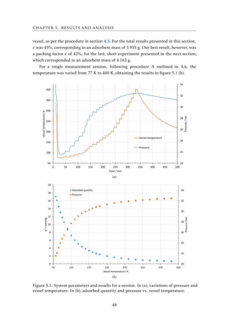
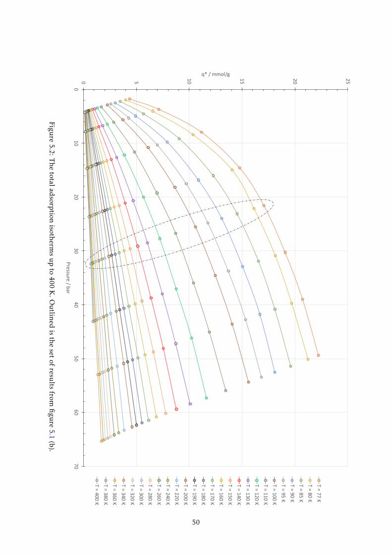
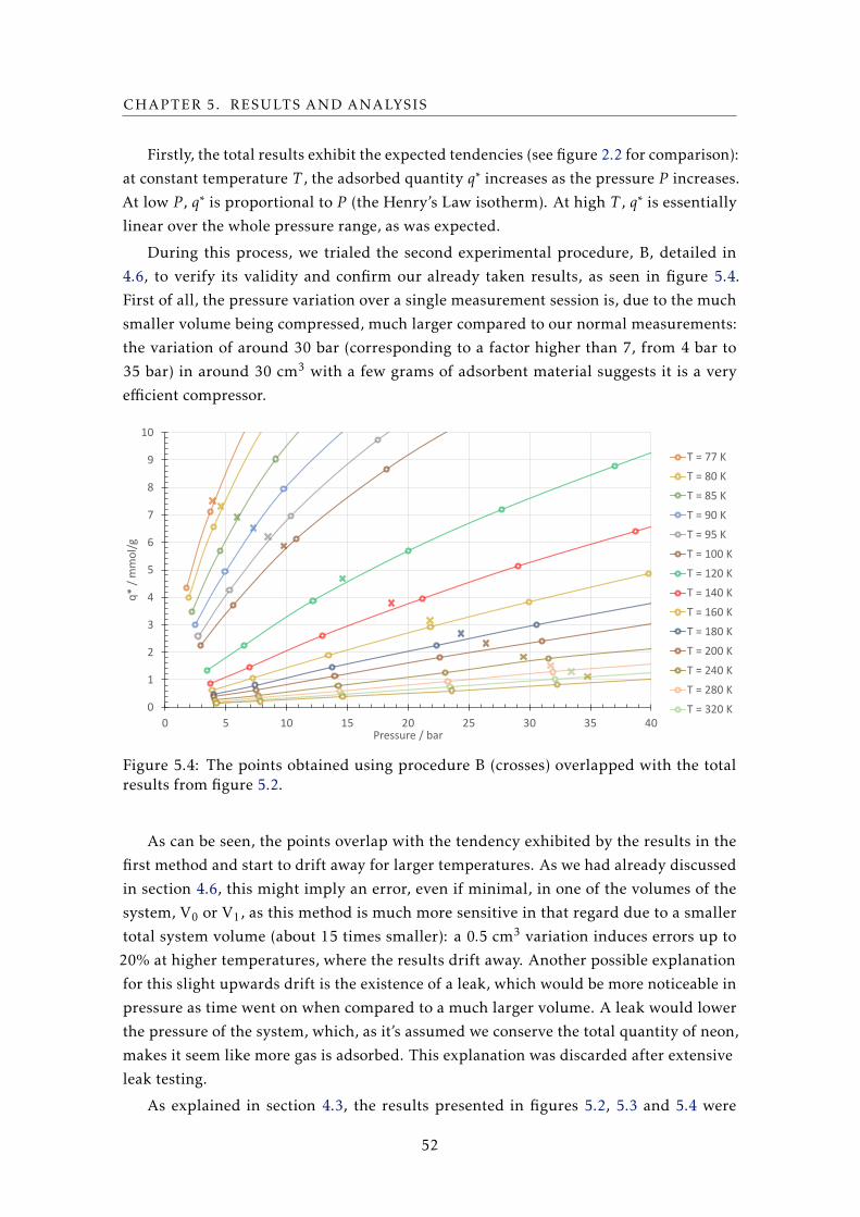
5.1 The percentual effect on the adsorbed quantity q∗ at the temperature and
pressure extremes of measurement when given errors are made. . . . . . . . 54
xvii
Chapter
1Introduction
One of the most important applications of space cryogenics is the cooling of infrared
detectors in satellites with a wide array of purposes. The recent years saw, in Europe, the
development of active coolers that are capable of providing significant cooling power at
an operational temperature of around 50 K, to meet Earth infrared observation mission
requirements. In the case of missions for space observation, such as, for example, the
Infrared Space Interferometer Darwin, these detectors enable the precise search of other
Earth-like worlds and analysis of their biological properties, as well as other astrophysical
objects in a similar wavelength range [1]. It’s within the optimization of these types of
applications that the cooling of the detectors is of great importance. The most advantages
are gathered by the so-called vibration-free coolers, cryocoolers that function without
moving parts and so do not induce unwanted vibrations that negatively affect the infrared
detection system.
In general, the compressor is the biggest source of vibrations in a cryocooler: a
vibration-free cooler must then invariably use a vibration-free compressor. A possibility
is the use of a sorption compressor, which, as opposed to mechanical compressors, works
thermochemically: this difference is enough to eliminate or minimize unwanted
vibrations during its functioning. One of the researched options for this application is
the use of this type of compressor to enable a Joule-Thomson effect. Such a
Joule-Thomson, vibration-free cryocooler is to be developed in a European Space Agency
project. The objectives of this project are to design, manufacture and test what’s called
an Elegant Breadboard Model of a vibration-free cooler that can provide active cooling for
temperatures in the range of 40 K to 80 K in order to answer the needs of potential
future Earth observation infrared missions [2]. It is in this context that the study of
adsorption materials to be used in the compressor was necessary.
1
CHAPTER 1. INTRODUCTION
This document will approach the work done in the design, development and testing
of a system for adsorption measurements, with the intention to provide useful data on
different adsorbent materials to aid the design and construction of an efficient adsorption
compressor for a vibration-free Joule-Thomson cooler. This dissertation is split into five
other chapters.
In chapter 2, the objectives of the work carried out and the project within which
it is inserted are described. With an intention to lay the groundwork for an accurate
understanding of the rest of the document, a general contextualization on the adsorption
phenomenon and its different types, theories and applications in the field of cryogenics,
with an emphasis on cryocoolers, is exposed, as well as a description of the sample used
to validate the system.
In chapter 3, an overview of the various experimental methods for the measurement
of adsorption properties, as well as a literature review pertaining to the most recent and
pertinent adsorption results to the developed system are carried out.
In chapter 4, the most important aspects of the volumetric experimental setup that was
developed are explored. After an initial summary of the layout and its key components,
the dimensioning - from general design to volumes and thicknesses, considering the high
pressures reached - is detailed for all these components: the adsorption vessel and the
calibrated volume, as well as the cooling and heating system designed to cover the 77
K to 500 K range. The preparation of the vessel and the sample prior to mounting in
the system is explained. A brief description of the LabVIEWTM interface is also given,
highlighting the automatic stabilization algorithm and the data acquisition system. Also
included in this chapter are step-by-step descriptions of the experimental procedures,
as well as an overview of the helium measurements of the system’s volumes, which are
fundamental for a later result analysis. A small section on the empty-vessel tests carried
out with an aim to pre-validate the system elaborates on experiments made without
an adsorbent sample, in an attempt to confirm the volumes present in the system by
performing routine measurements.
In chapter 5, the results for adsorption of neon on HKUST-1 are presented, most
notably in the form of adsorption isotherms, from which important data such as the
isosteric curves, the heat of adsorption, and others can be derived. A quantitative error
and correction analysis is performed to gauge possible sources of error or corrections
and their influence. Our results are compared with those obtained by a commercial
gravimetric system belonging to LATPE, a partner laboratory in the Chemistry
Department, and with results for adsorption heat obtained by another group in 2013, as
a means to validate our system.
Finally, in chapter 6, general considerations and conclusions taken from this work, as
well as what to improve about the system in the near future.
The appendix includes all the drawings for important pieces that were engineered
during the development of the system.
2
Chapter
2Contextualization
2.1 Vibration-free cooler in the 40 – 80 K range
In 2014, the European Space Agency posted an Announcement of Opportunity detailing
specified requirements for the “Development of a 40 K to 80 K vibration-free cooler”.
This project was assigned to two companies, one of them being Active Space
Technologies: a Portuguese company specialized in thermo-mechanical and electronics
engineering for aerospace, defense, automotive, nuclear fusion and scientific
applications. It is currently in progress in collaboration with the Cryogenics Laboratory
and the Adsorption Technology Group (LATPE), both located in the Faculdade de
Ciências e Tecnologia of the Universidade Nova de Lisboa (FCT-UNL). From it originated
a Ph. D. thesis (J. Barreto, for the development of a functioning prototype), and two M.
Sc. theses (adding to this one, M. Baeta, for the development of the nitrogen stage).
The cooler is projected to be of the Joule-Thomson type, split in two stages, one with
nitrogen and another with neon (cooling power: 0.5 W at 80 K and 40 K, respectively).
It’s predicted to cover most of the 40 K to 80 K range. To avoid the vibration induced
by the more common mechanical compressors used for gas compression, the compressor
will be sorption-based. Advantages of the latter are discussed in a later section about
cryocoolers.
The design and development of a system for adsorption measurements is then
necessary for a more precise dimensioning of the adsorption compressor used in the
project’s cryocooler. For the first measurements taken on the system, the adsorbent
sample was HKUST-1, a metal-organic framework that’s attractive due to properties
close to the desired ones and its commercial availability. The adsorbate gas used in the
measurements was neon, the working fluid of the second stage of the cryocooler, due to,
when compared to nitrogen, a lack of experimental data using HKUST-1 and its lower
3
CHAPTER 2. CONTEXTUALIZATION
tendency to adsorb. A brief description of the adsorbent is available in a later section.
2.2 Adsorption
Adhesion of any atoms, ions, or molecules provenient from a fluid to a surface is defined
as adsorption. The process creates a layer of adsorbate on the adsorbent, at surface level.
This phenomenon can be explained by the existence of a negative surface energy,
which is the driving force behind any surface phenomena: in a material, the surface
atoms, which are not wholly surrounded by other adsorbent atoms, are more susceptible
to binding with surrounding bodies due to this unbalanced and asymmetric configuration
in comparison to the bulk atoms. The attracted particle (adsorbate) then fills in the
pores on the surface of the solid (adsorbent) when this phenomenon occurs. It’s worth
noting that surface energy caused by atomic force imbalance is not the only factor for the
characterization of adsorption properties, as the compatibility of pairs of adsorbents and
adsorbates (usually called adsorption working pairs) is defined by several other properties
[3], [4].
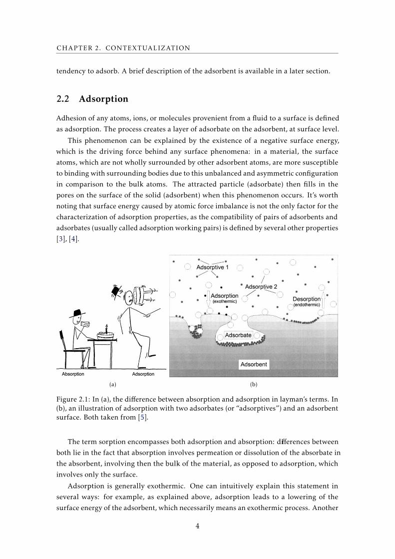
(a) (b)
Figure 2.1: In (a), the difference between absorption and adsorption in layman’s terms. In(b), an illustration of adsorption with two adsorbates (or “adsorptives”) and an adsorbentsurface. Both taken from [5].
The term sorption encompasses both adsorption and absorption: differences between
both lie in the fact that absorption involves permeation or dissolution of the absorbate in
the absorbent, involving then the bulk of the material, as opposed to adsorption, which
involves only the surface.
Adsorption is generally exothermic. One can intuitively explain this statement in
several ways: for example, as explained above, adsorption leads to a lowering of the
surface energy of the adsorbent, which necessarily means an exothermic process. Another
4
2.2. ADSORPTION
way to put it is to look at the equation for the Gibbs free energy, G, a thermodynamical
potential that’s minimized at chemical equilibrium at constant temperature and pressure:
that means a diminishing G signifies a spontaneous, or favored, reaction. This potential
was described by its eponym, J. W. Gibbs, as:
... the greatest amount of mechanical work which can be obtained from a
given quantity of a certain substance in a given initial state, without increasing
its total volume or allowing heat to pass to or from external bodies ... [6]
Its general definition is:
G(P ,T ) =H − T S (2.1)
where G is the Gibbs free energy, P the pressure, T the temperature, H the enthalpy,
and S the entropy, all pertaining to a closed system.
So, at constant temperature:
∆G = ∆H − T∆S (2.2)
Saying adsorption is exothermic is the same as saying the variation of enthalpy, ∆H ,
associated with adsorption is negative. Moreover, since the adsorption of a gas implies the
restriction of its movement, an adsorption intuitively leads to a decrease in the entropy of
the gas, and thus ∆S is negative. For the process to be spontaneous, or ∆G negative, seeing
as ∆S is negative, ∆H must be necessarily negative enough to cancel out the positive
−T∆S term. Therefore, adsorption is generally exothermic, always for physisorption in
particular but not necessarily for certain variants of chemisorption, however [7]. These
two types of adsorption will be explained in subsection that follows.
2.2.1 Types of adsorption
Adsorption processes are mostly distinguished by the nature of the bonding processes
involved, being usually characterized as chemical adsorption (or chemisorption) or
physical adsorption (or physisorption). The distinction is basically the same as one
between general chemical and physical interactions, and is sometimes difficult to make
for some intermediate cases, such as strong hydrogen bonding [8] or weak charge
transfers. This often complicates the modelling and analysis of a given system, since the
methods for doing so vary depending on whether the phenomenon is chemical or
physical. As will be elaborated below, the magnitude of the energies involved in each
type of adsorption are very disparate, and so often times it is pertinent and helpful to
calculate the adsorption enthalpy, for example, as to get a clearer picture [9].
5
CHAPTER 2. CONTEXTUALIZATION
2.2.1.1 Chemisorption
In this type of adsorption, the adsorbate reacts chemically with the adsorbent, becoming
chemically bonded with it: this means that the chemical structure of the material’s surface
is altered, so generally only one layer – a monolayer – of a given adsorbate will form. It’s
a very selective process, depending heavily on the chemical nature of both adsorbent
and adsorbate. The forces involved have a very short range, as characteristic of chemical
bonds. Also to note is that this process is often irreversible, making it impossible to
remove the adsorbed gas without altering the surface. Chemisorption has extremely high
bond enthalpies: between 250 kJ/mol and 500 kJ/mol. In general, this very large enthalpy
makes the use of this type of adsorption not viable for adsorption compressors. This is
the main difference to physisorption.
2.2.1.2 Physisorption
Unlike chemisorption, physisorption occurs when the adsorbate remains on the
adsorbent’s surface due to weak, long-range Van der Waals or London forces. Since the
binding energies involved are relatively weak (less than 20 kJ/mol), it’s heavily
influenced by temperature and pressure of the system: since physisorption is an
exothermal process, low temperatures and high pressures contribute to adsorption,
while high temperatures and low pressures lead to desorption. Due to the long-range of
the forces and the non-chemical nature of these processes, it’s possible to have
multilayered adsorption as long as the forces involved allow it.
Within the context of this thesis, physisorption will be the sole focus, and so any
mentions of adsorption from this point on refer to the physical, and not the chemical,
type.
The exothermic property of physisorption mentioned earlier in this section is crucial
to the functioning of an adsorption compressor and its quantification through the heat of
adsorption will be done in the result analysis.
6
2.2. ADSORPTION
2.2.2 Theoretical formulations
To this date, at least 15 different isotherm models have been developed for adsorption
studies. They have varying degrees of ideality and sophistication, as well as different
cases in which they are applicable or not [10].
One of the simplest and most versatile models to date was derived by Langmuir, in
1918. This adsorbate-adsorbent system was treated by making several assumptions:
• The adsorbate behaves as an ideal, classical gas;
• The adsorbent surface is perfectly flat and homogeneous;
• The adsorbate becomes immobile after adsorbing;
• All the adsorption sites are equivalent;
• There are no interactions between adsorbed molecules.
The system is basically treated as a chemical system – though the reaction is not
necessarily chemical – with reactions occurring for adsorption and desorption. The
reagents are considered the free adsorbate molecules and the open adsorbent sites, and
the products the adsorbent’s occupied sites. Equalizing the chemical potentials of these
two states, the central equation for the Langmuir model can be derived, which gives the
percentage of filled adsorbent sites θ as a function of the gas pressure PA:
θ =KPA
1 +KPA(2.3)
where K is a constant, dependent on reaction heat, particle mass and temperature.
Equation 2.3 leads to the so-called Langmuir isotherms of adsorption, figure 2.2:
0
0.1
0.2
0.3
0.4
0.5
0.6
0.7
0.8
0.9
1
0 20 40 60 80 100
Fille
d s
ites
θ
Pressure PA
T
Figure 2.2: Example of typical Langmuir isotherms. For the same pressure, the highestθsignifies a lower temperature (as in, more adsorption at lower temperatures!).
7
CHAPTER 2. CONTEXTUALIZATION
It’s interesting to note that the isotherms for high temperatures (which would be
the lower adsorbed quantities θ in figure 2.2) exhibit a linear behavior with respect to
pressure, while the isotherms for lower temperatures, where adsorption is more favored,
exhibit much earlier saturation. This saturation reduces the effect of pressure at high
pressures, as the adsorbent material’s sites are then almost completely filled with the
adsorbate gas. At low pressures, θ is proportional to PA, which is called Henry’s Law.
This experimental law is confirmed by the limit of low pressure of the Langmuir model.
To understand the adsorption process, it’s also important to know that it results in
dynamic equilibrium: a coexistence of free molecules and adsorbed molecules, where
both adsorption and desorption are constantly happening at the same rate. This can be
described by equation 2.4, where the rates of adsorption and desorption are equaled:
K =KaKd
=[AB]
[A][B]→ K =
θ(1−θ)PA
(2.4)
where [A] is the quantity of free gas molecules (proportional to PA), [B] the quantity
of unoccupied surface atoms (proportional to 1 − θ) and [AB] the quantity of adsorbed
gas molecules (proportional to θ). Ka and Kd are the rates of reaction of adsorption and
desorption, respectively. Rearranging equation 2.4, we obtain the former equation 2.3.
This model is widely used, both educationally and experimentally: it is applicable
in most chemisorption phenomena as well as physisorption below a given saturation
pressure, giving it versatility. Other models that take, for instance, multilayers (Brunauer-
Emmett-Teller, or BET for short, often used to estimate adsorbent surface areas [11]),
larger incidence of adsorption near already adsorbed molecules (Kisliuk [12]), and other
factors into account, exist for applications where a higher degree of analysis is required.
Another important theoretical aspect is the calculation of the heat of adsorption. As
already mentioned, adsorption leads to a dynamic equilibrium, and is an exothermal
process, which means a molecule of gas transfers heat to its surroundings when it is
adsorbed. By treating adsorption as a change of phase and the gas as ideal, we can apply
the Clausius-Clapeyron equation to calculate the reaction heat (equation 2.5) [13]:
L = −Rδ(ln(P ))
δ(
1T
) (2.5)
where L is the reaction heat, R the ideal gas constant, P the pressure and T the
temperature of the system.
One important thing to keep in mind is that, in the specific case of adsorption, L is
conventionally taken at isosteric conditions, meaning at constant adsorbed quantities θ.
Essentially, the slope of an isosteric curve, which would be a horizontal line in figure 2.2,
plotted with ln(P ) and 1T , will give us the adsorption heat. This slope should be negative,
as we concluded earlier from ∆H in equation 2.2.
This heat, as well as the isotherms, taken over the pressure range, are the two
important parameters for the design of a working gas adsorption compressor.
8
2.2. ADSORPTION
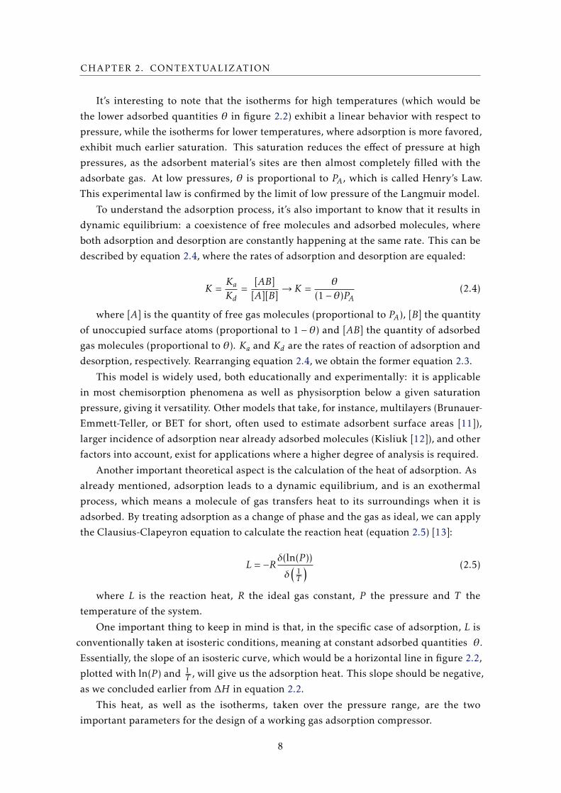
2.2.3 HKUST-1 and other adsorbents
Currently used adsorbents can be split into several categories, depending on their typical
surface area (which is always relatively large) and their intended and diverse applications:
these can be industrial, medical, scientific, among others.
(a) (b)
Figure 2.3: In (a), activated carbon [14]. In (b), zeolite [15]. These are the two most usedand commercialized types of adsorbents.
The most widely popular and commercialized adsorbent in cryogenics is activated
carbon, a form of carbon processed in such a way that it has small, low-volume pores
that give the material an enormous surface area: typically around 1000 m2/g and as high
as 3000 m2/g [5]. The raw carbon is extracted from common carbonaceous materials
such as nutshells, wood, and coal. The extraction is often called carbonization, and is
performed through pyrolisis (thermochemical decomposition of organic materials in an
inert environment) in the temperature range from 600 ºC to 900 ºC. The carbon
product’s surface area is then enhanced through physical or chemical means, called
activation. In the physical case, this means exposure to an oxidizing atmosphere at very
high temperatures (600 ºC to 1200 ºC), while in the chemical case, it means
impregnation of the raw material with certain strong chemicals. A convenient property
of activated carbon is that it has a great variety of heavily researched methods for its
regeneration, such as ultrasound [16], electrochemical [17] and microwave-assisted [18]
methods, not necessarily requiring high temperatures to desorb all the gas it holds.
Other very common commercialized adsorbents are zeolites, which are microporous,
aluminosilicate minerals that, due to their very regular molecular-sized pore structure,
have the ability to only allow adsorption to molecules smaller than a given size. This
ability puts this material in the family of solids known as molecular sieves and makes
them very attractive for molecular separation and trapping. The typical surface areas are
around 500 m2/g.
9
CHAPTER 2. CONTEXTUALIZATION
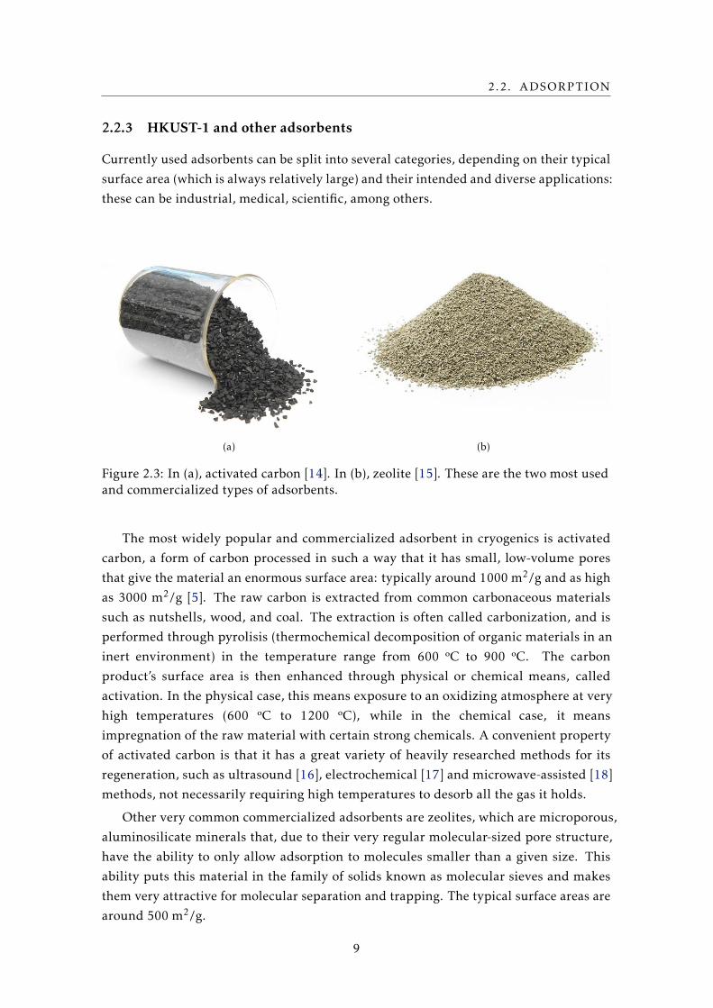
HKUST-1, the material used to make measurements with the developed system, is an
adsorbent categorized as a metal-organic framework and available under the commercial
name BasoliteTM C300, manufactured by Sigma Aldrich (Germany). Its chemical
denomination is Cu3(BTC)2. Table 2.1 summarizes and highlights some interesting
properties as an adsorbent of this commercialized variant of HKUST-1.
Table 2.1: Physical properties of BasoliteTM C300, adapted from [19].
Property HKUST-1
Activation conditions 423 K under vacuum (10 h)Molecular weight 605 g/molParticle size 16 µmBulk density 350 kg/m3
BET surface area 1500 to 2100 m2/g
This material was one of options for the project’s adsorption compressors due to its
capacity in adsorbing both nitrogen and neon better than activated carbon. As already
mentioned in section 2.1, adsorbing neon is conventionally less favorable: this is due to
its little or no ability to react when compared to non-noble gases. It was tested on due
to its quick availability when compared to the other analyzed metal-organic frameworks,
that were both not commercial and not simple to synthesize.
(a) (b)
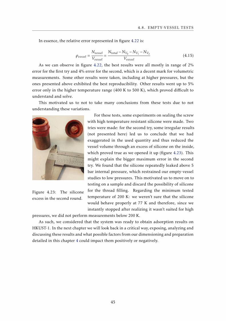
Figure 2.4: In (a), HKUST-1 in its powder form, as it is provided commercially. Notethe darker and lighter hues of blue, corresponding to different states of oxidation(reversible). In (b), the molecular framework of HKUST-1, with spheres representingthe pore sizes within it that can be used for gas storage. The green sphere has a diameterof approximately 10 Å. [20]
These conclusions were attained through simulations done by Prof. J. P. Mota, from
LATPE, who analyzed several possible adsorbent samples for the working gases [21].
10
2.2. ADSORPTION
2.2.4 Applications in cryogenics
2.2.4.1 Cryocoolers
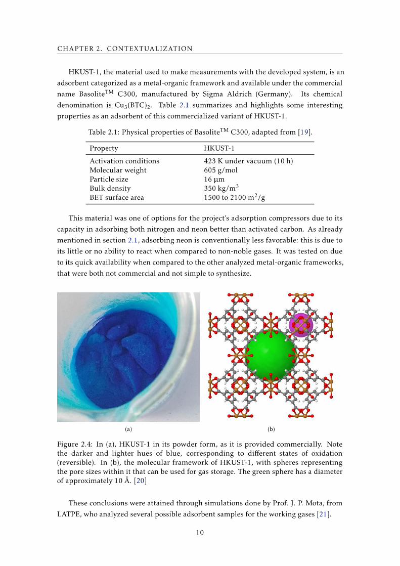
Adsorption is usually not the concept directly behind any type of cooling. However, it can
be used in several types of cooling cycles through sorption-based compressors [22], where
the pressure cycles are generated through heating and cooling cycles of adsorbent-filled
containers, generally called adsorption vessels. These compressors have the advantage
that they do not have any moving parts, which severely minimizes their vibrations and
wear due to use: this makes them attractive for a great variety of applications, where
lifetime and the lowest possible level of vibrations are an important factor [23], such as
in the project in which this thesis is inserted.
Figure 2.5: Schematic of a generic Joule-Thomson cryocooler using adsorptioncompressors [1] a.
aReprinted from Cryogenics, Vol. 42, nr. 2, J. F. Burger et al, Vibration-free 5 K sorption cooler for ESA’sDarwin mission, pp. 97–108, Copyright 2002, with permission from Elsevier.
For example, within the scope of the already mentioned project, the functioning of a
Joule-Thomson sorption cooler (figure 2.2.4.1) will be detailed to illustrate the importance
of the compressor and its control.
As the name suggests, a Joule-Thomson cryocooler takes advantage of the
Joule-Thomson effect to cool a working fluid. This effect, also known as a throttling
process, consists of the temperature change of a real (as opposed to ideal) fluid when
forced through a thermally insulated restriction, which results in a (Joule-Thomson)
expansion. This results in cooling or heating depending on the fluid’s thermodynamic
properties. The thermally insulated restriction is considered a small enough channel or
orifice to force a large pressure change. Since no heat is exchanged with the
surroundings, it can be proven that this process is isenthalpic (∆H = 0).
11
CHAPTER 2. CONTEXTUALIZATION
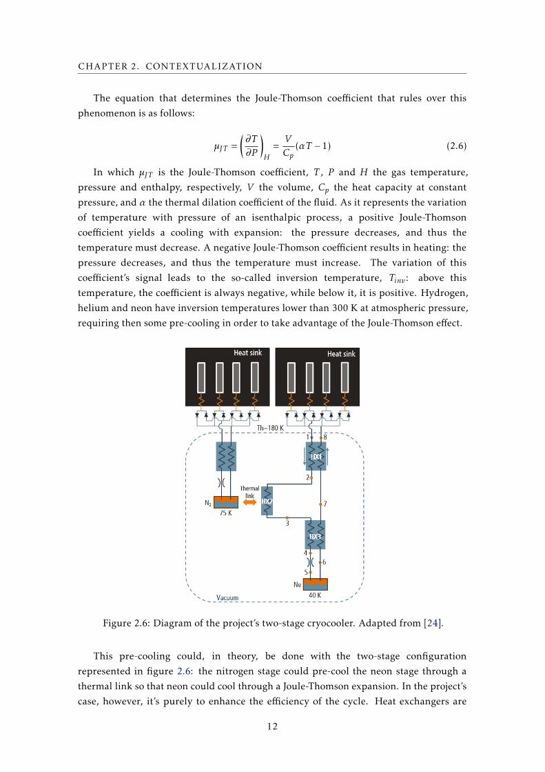
The equation that determines the Joule-Thomson coefficient that rules over this
phenomenon is as follows:
µJT =(∂T∂P
)H
=VCp
(αT − 1) (2.6)
In which µJT is the Joule-Thomson coefficient, T , P and H the gas temperature,
pressure and enthalpy, respectively, V the volume, Cp the heat capacity at constant
pressure, and α the thermal dilation coefficient of the fluid. As it represents the variation
of temperature with pressure of an isenthalpic process, a positive Joule-Thomson
coefficient yields a cooling with expansion: the pressure decreases, and thus the
temperature must decrease. A negative Joule-Thomson coefficient results in heating: the
pressure decreases, and thus the temperature must increase. The variation of this
coefficient’s signal leads to the so-called inversion temperature, Tinv : above this
temperature, the coefficient is always negative, while below it, it is positive. Hydrogen,
helium and neon have inversion temperatures lower than 300 K at atmospheric pressure,
requiring then some pre-cooling in order to take advantage of the Joule-Thomson effect.
Figure 2.6: Diagram of the project’s two-stage cryocooler. Adapted from [24].
This pre-cooling could, in theory, be done with the two-stage configuration
represented in figure 2.6: the nitrogen stage could pre-cool the neon stage through a
thermal link so that neon could cool through a Joule-Thomson expansion. In the project’s
case, however, it’s purely to enhance the efficiency of the cycle. Heat exchangers are
12
2.2. ADSORPTION
constant presences in these cryocoolers to facilitate pre-cooling and increase the cooler
efficiency, as well as any other heat transfers present in the system. Despite being a part
of the project, these elements will not be discussed in detail within this thesis, as they are
not present in the developed adsorption measurement system (M. Baeta, M. Sc. thesis).
Sorption compressors are cyclical systems in which the adsorption vessels alternate
between adsorption and desorption (respectively, lowering and raising pressure) through
the variation of temperature. As already mentioned in the description of physisorption,
temperature has a strong influence in these phenomena. However, to avoid strong
fluctuations of gas flow, which are harmful to the temperature stability of the
Joule-Thomson cycle, one needs at least four vessels, functioning out-of-phase with each
other, with adequate check valves [1].
(a) (b)
Figure 2.7: Working cycle of a 5 K Joule-Thomson cryocooler’s adsorption compressor,taken from [1] a. In (a), the cycle drawn over generic adsorption isotherms. In (b), thevariation of the several system parameters over the cycle.
aReprinted from Cryogenics, Vol. 42, nr. 2, J. F. Burger et al, Vibration-free 5 K sorption cooler for ESA’sDarwin mission, pp. 97–108, Copyright 2002, with permission from Elsevier.
A typical compressor cycle is shown in figure 2.2.4.1 and corresponds to the cryocooler
schematized in figure 2.2.4.1. In a first phase, A, a vessel is warmed up, which results
in desorption. This compresses the gas, raising the pressure, which upon reaching a
certain value (in the example, 30 bar) opens the high pressure check valve (see figure
2.2.4.1), resulting in a flow of desorbed gas exiting the vessel towards the expansion valve
in a second phase, B. In a third phase, C, the heating is closed and the vessel connected
through a heat switch to a cold source (heat sink), leading to a cooling of the vessel and
consequent adsorption, which decompresses the gas, lowering the pressure: this closes
the high pressure check valve. As the pressure reaches the low pressure check valve
13
CHAPTER 2. CONTEXTUALIZATION
limit (in the example, 1 bar), the valve opens, which establishes a flow of adsorbing gas
entering the vessel from the expansion valve in a fourth phase, D. Two pairs of vessels
operating in opposed phase manage to damp the flow fluctuations inherent to this cycle.
2.2.4.2 Cryopumps
In the field of vacuum technology, cryopumps are a constant presence in high and ultra-
high vacuum systems. They are clean, fast vacuum pumps that work through removal of
gases and vapors through condensation and adsorption on cold surfaces.
Condensation of particles on the cold surface happens when the vapor pressure of a
given gas at the given cold temperature is so low that the condensed phase forms,
effectively removing the gas particle from the system’s volume. Unfortunately, the
condensation of neon, hydrogen and helium is impossible with most cryopumps,
because the vapor pressure of the former two at 20 K (the temperature limit for a
relatively simple and usual cryocooler) is considerably high and the liquid phase for
helium appears only below 5 K. The adsorption of these gases, however, doesn’t suffer
from this temperature limitation, which makes it a very good complement to the
condensation process, making this a relatively effective pump for all types of gases, yet
with some limitations for helium.
Figure 2.8: Vapour pressure vs. temperature for common pumped gases [25] a
aReprinted from Vacuum, Vol. 30, nr. 30, P. D. Bentley, The modern cryopump, pp. 145–158, Copyright1980, with permission from Elsevier.
Let us keep in mind that these phenomena of condensation and adsorption cannot
14
2.2. ADSORPTION
occur for an infinite number of particles, or an infinite amount of time, without “cleaning
out” the system: this process, called regeneration, involves the warming of the cryopump
to a high temperature, allowing the trapped gases and vapours to go back to a gaseous
state, being then removed from the system by the appropriate pumping system.
2.2.4.3 Heat switches
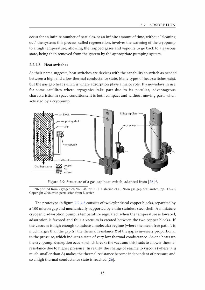
As their name suggests, heat switches are devices with the capability to switch as needed
between a high and a low thermal conductance state. Many types of heat-switches exist,
but the gas gap heat switch is where adsorption plays a major role. It’s nowadays in use
for some satellites where cryogenics take part due to its peculiar, advantageous
characteristics in space conditions: it is both compact and without moving parts when
actuated by a cryopump.
Figure 2.9: Structure of a gas gap heat switch, adapted from [26] a.
aReprinted from Cryogenics, Vol. 48, nr. 1, I. Catarino et al, Neon gas-gap heat switch, pp. 17–25,Copyright 2008, with permission from Elsevier.
The prototype in figure 2.2.4.3 consists of two cylindrical copper blocks, separated by
a 100 micron gap and mechanically supported by a thin stainless steel shell. A miniature
cryogenic adsorption pump is temperature regulated: when the temperature is lowered,
adsorption is favored and thus a vacuum is created between the two copper blocks. If
the vacuum is high enough to induce a molecular regime (where the mean free path λ is
much larger than the gap ∆), the thermal resistance R of the gap is inversely proportional
to the pressure, which induces a state of very low thermal conductance. As one heats up
the cryopump, desorption occurs, which breaks the vacuum: this leads to a lower thermal
resistance due to higher pressure. In reality, the change of regime to viscous (where λ is
much smaller than ∆) makes the thermal resistance become independent of pressure and
so a high thermal conductance state is reached [26].
15
Chapter
3State of the art
3.1 Experimental methods
To dimension a system, the characteristic adsorption isotherms (for instance, figure
2.2.4.1, bottom left, X(T ,P )) must be known. It is on this topic that a small overview of
adsorption measurement methods currently in use is done in this chapter, with historic
contextualization and current developments in each of them. The overview on
experimental methods is based heavily on [5].
3.1.1 Volumetric method
The volumetric (or manometric) method is considered the pioneer of adsorption
measurements, with early experiments situated in the late 1700s up to the early 1900s. A
prototype of what is the current typical setup was developed and established in the
1940s.
It consists on the principle that if a given quantity of gas is well known, it can be
expanded into a pre-evacuated vessel with an adsorbent sample in it. As the expansion is
carried out, the quantity of gas is split into partially adsorbed on the adsorbent and
partially remaining in the proximity of the adsorbent in a gaseous state. Through
conservation of mass and knowledge of the void volume (the volume in which the
adsorbate gas can enter), the amount of gas being adsorbed can be calculated.
The measurement is conventionally done through the variation of the equilibrium
pressure from the initial state, where a calibrated, well-known volume is filled with a
given quantity of gas, to the final state, where the initial quantity of gas has expanded to
an adsorption vessel containing an adsorbent material, and has partially adsorbed. One
can immediately relate a change in pressure inside the two known volumes to a change
in quantity of gas through an equation of state, usually the ideal gas equation, depending
17
CHAPTER 3. STATE OF THE ART
on the particularities of the system. This change in gas quantity is the adsorbed quantity,
as adsorbed particles don’t contribute to gas pressure. Because the pressure measurement
is the key of this determination, the name “manometric” is also conventionally used.
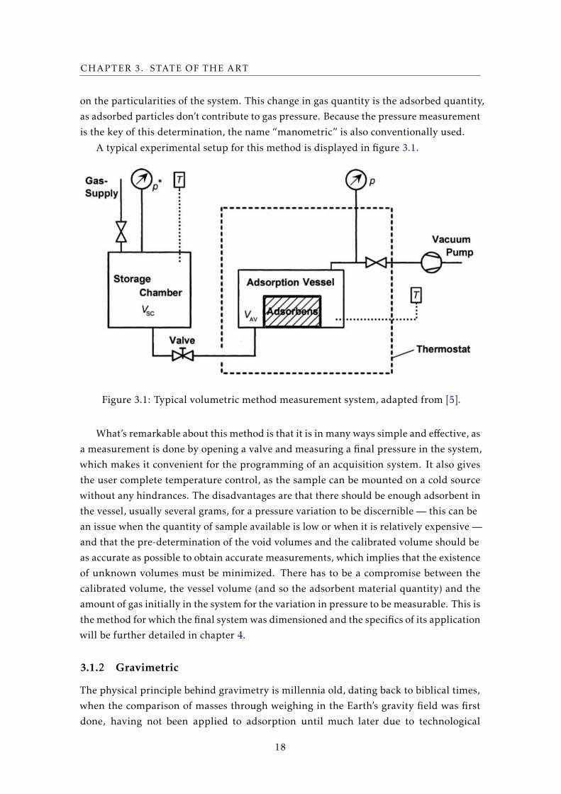
A typical experimental setup for this method is displayed in figure 3.1.
Figure 3.1: Typical volumetric method measurement system, adapted from [5].
What’s remarkable about this method is that it is in many ways simple and effective, as
a measurement is done by opening a valve and measuring a final pressure in the system,
which makes it convenient for the programming of an acquisition system. It also gives
the user complete temperature control, as the sample can be mounted on a cold source
without any hindrances. The disadvantages are that there should be enough adsorbent in
the vessel, usually several grams, for a pressure variation to be discernible — this can be
an issue when the quantity of sample available is low or when it is relatively expensive —
and that the pre-determination of the void volumes and the calibrated volume should be
as accurate as possible to obtain accurate measurements, which implies that the existence
of unknown volumes must be minimized. There has to be a compromise between the
calibrated volume, the vessel volume (and so the adsorbent material quantity) and the
amount of gas initially in the system for the variation in pressure to be measurable. This is
the method for which the final system was dimensioned and the specifics of its application
will be further detailed in chapter 4.
3.1.2 Gravimetric
The physical principle behind gravimetry is millennia old, dating back to biblical times,
when the comparison of masses through weighing in the Earth’s gravity field was first
done, having not been applied to adsorption until much later due to technological
18
3.1. EXPERIMENTAL METHODS
restraints. The gravimetric method as it is applied today, concerning adsorption
phenomena of gases on solids, is then relatively recent, from the second half of
the 1900s.
The method is based on the fact that an adsorbent on which an adsorbate accumulates
undergoes a variation in mass, equal to the mass of the adsorbed gas. Thanks to noticeable
improvements of weighing techniques and microbalance quality, this method is nowadays
very sensitive. Within the gravimetric methods, different variants can be distinguished,
dependent on the type of balance used, whether the balance is a single or double beam
type, and the temperature region exploited.
Figure 3.2: Typical gravimetric method measurement system, adapted from [5].
Though there are no corrections for void volumes to be done, the fact that the sample
is usually immersed in the adsorbate gas requires a correction for the apparent weight it
takes on due to buoyancy (Archimedes principle), depending on the gas density in the
sample chamber. Another disadvantage is the cost and sophistication of such a system,
when compared to its manometric counterpart. There is also the problem that
temperature control can be more complicated due to the sample being on a balance,
which makes cooling only possible through cryogenic liquids, with the disadvantages
that entails when opposed to a connection to a cryocooler’s cold finger. There is also no
longer the issue of the gas adsorbing on the wall, since the measurements are done
purely on the adsorbent. Advantages include a much greater sensibility due to greatly
reduced elements of error, the relatively little amount of adsorbent material required,
and that a great insight into the kinetics of adsorption can be obtained with
Several other recent methods exist besides the two aforementioned ones, with varying
levels of popularity and divulgation. Again, most of this subsection is mainly based
on [5].
Volumetric-gravimetric systems are systems in which the two previously described
methods are applied simultaneously, in order to both conjugate the advantages of the two
and to be able to determine coadsorption equilibria of gas mixtures without requiring a
chromatograph or mass spectrometer. They are specially applied to industrial process
control and design.
The oscillometric method, or oscillometry, consists of a pendulum or a freely floating
rotator in slow rotational oscillation, coated with adsorbent material, where the damping
of the movement of the chosen structure in a surrounding adsorbate is due to both the
adsorption phenomenon and the friction with the gas. Measurements can be made
optically, to gauge the movement properties of the structure in use. The chamber is in a
thermostatic bath, which brings the same disadvantage as the gravimetric method: lack
of good sample temperature control.
The impedance spectroscopy method relies on the basis that, if a static or alternating
electric field is applied to a weakly electrical conducting or dielectric material — which
encompasses most activated carbons, materials typically used for adsorption studies —
the electrons and nuclei of the components are shifted in opposite directions to each
other. This induces dipole moments in the material, which are measurable through the
capacitance C or impedance Z of capacitors filled with the material in question. One
gets C(f) or Z(f) curves, where f is the frequency of the applied electric field, which
are characteristic for the adsorbent material in vacuum and for adsorbent/adsorbate
systems. Through pre-calibration with the aid of other methods, such as manometric or
gravimetric, one can obtain a curve that relates capacitance or impedance to quantity of
adsorbed gas. This makes impedance spectroscopy also highly automatable, sharing the
rest of the advantages and disadvantages of gravimetry.
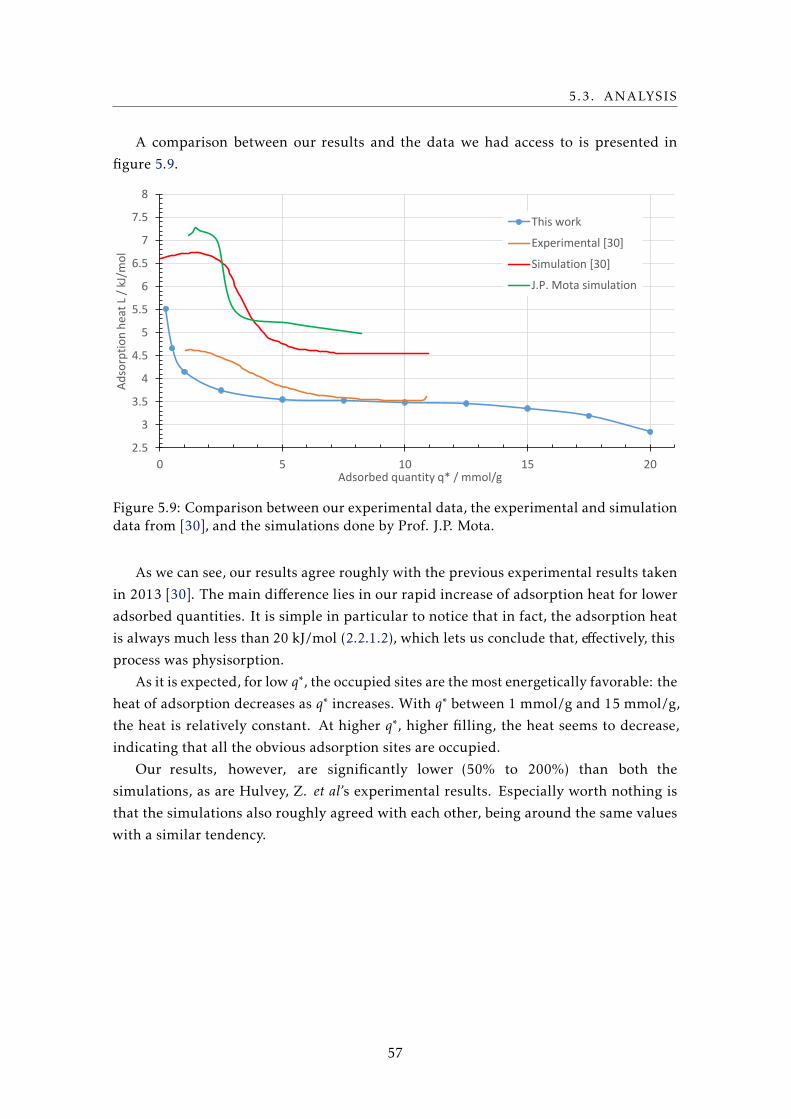
3.2 Literature review of adsorption data on HKUST-1
In this section, there is a succinct review of published work done by other groups that is
pertinent to our goals. This means, essentially, volumetric measurements in high
temperature and pressure conditions compared to the usual range, performed in
HKUST-1.
First of all, as mentioned in [27], from 1984, a hefty amount of experimental data
for low-pressure cryogenic adsorption exists due to applications of adsorbents in cryo-
pumping and low-pressure gas removal processes. Due to HKUST-1 and other types of
metal-organic frameworks having not yet been developed at that time, the sample used
for this work was activated carbon, which we’ve already concluded to have relatively
20
3.2. LITERATURE REVIEW OF ADSORPTION DATA ON HKUST-1
lesser performances for neon and nitrogen adsorption. Chan, C.K. et al, however, shared
our goal of application in adsorption compressors, and thus covered a large range of
temperatures and pressures (77 K to 400 K, 1 atm to 80 atm).
More recently, in 2011, Moellmer, J. et al also treated high-pressure adsorption (up to
500 bar), this time for HKUST-1, using however a much smaller temperature range (273
K to 343 K) [28]. These were, at the time, reported to be the first high-pressure (over200
bar) measurements done on this sample. As explained in the paper’s introduction and to
further explain the lack of extensive literature on this topic, most of HKUST-1’s current
applications lie in the lower pressure range: at the time of publishing and to the best of
their knowledge, the only other literature found for high pressure adsorption
measurements on HKUST-1 was a volumetric and gravimetric analysis of methane
adsorption in a group of metal-organic frameworks [29], going up to 200 bar.
In 2013, an interesting study on noble gas adsorption in HKUST-1, experimental and
computational [30], provides us with values for adsorption heats for neon adsorption,
with which we’ll compare our results in addition to the ones simulated and obtained by
LATPE in subsection 5.3.3.
In 2014, Raganati, F. et al analyzed CO2 capture in HKUST-1 in a sound assisted bed
[31], having in parallel confirmed several physical properties. The most interesting in our
perspective was a thermogravimetric analysis which gives us a reasonable profile of the
behavior of the material with temperature, giving us an absolute maximum temperature
limit of circa 350 ºC (see figure 3.2). This motivated us to perform a thermogravimetric
analysis to confirm their results, since the temperature maximum is of great importance
to our measurements and the soldered sealing of our vessel (see section 4.3).
Figure 3.3: Thermogravimetric analysis of HKUST-1 in an N2 environment. Adaptedfrom [31] a.
aReprinted from Chemical Engineering Journal, Vol. 239, F. Raganati et al, CO2 capture performance ofHKUST-1 in a sound assisted fluidized bed, pp. 75–86, Copyright 2014, with permission from Elsevier.
21
CHAPTER 3. STATE OF THE ART
As already mentioned, the literature for this neon adsorption on HKUST-1 paired with
this range of temperatures and pressures was, to the best of our knowledge and at the time
of writing, not possible to be found. As such, our results, presented in chapter 5, expand
the usual temperature range of neon on HKUST-1 adsorption, and in specific providing
data for applications in the more extreme temperature and pressure range applications,
such as adsorption compressors, as in this project and the already mentioned work [27].
22
Chapter
4Experimental setup
4.1 System summary and the volumetric method
As mentioned in the former chapter, the volumetric method was chosen for our
measurements. A diagram summarizing the developed system is displayed in figure 4.1.
Vessel
DewarCalibrated
volumeGas bottle
Pressure sensor 2
Pressure sensor 1
Vvessel
V2
25 1V1
V0
Vacuum pump
E
3
4
B
A
C
D
Figure 4.1: Gas system of the built system. The Pt100 thermometer locations are givenby letters A through D.
The system consists of an adsorption vessel Vvessel , thermally protected inside a
liquid nitrogen dewar and equipped with a system for temperature control which will be
detailed in section 4.5. The vessel contains a certain quantity of adsorbent, and is
connected through a capillary to a gas manifold containing two pressure sensors and a
23
CHAPTER 4. EXPERIMENTAL SETUP
calibrated volume V2, used as a buffer and for the initial gas quantity determination.
Also connected to the manifold are the gas bottle, from which the sample adsorbate is
provided, and a rotary vacuum pump, for cleaning out the whole system.
Valves 1 and 2 are used for the supply of gas, 1 being the adjustable supply, so we
can establish a given initial pressure, and 2 a quarter-turn valve. Valve 3 is the pumping
valve, and valve E the escape valve, opened in the case of a non-pumpable pressure excess
in the system. Valves 4 and 5 constitute the interface between the calibrated volume and
the adsorption vessel. Operation of this manifold will be further discussed in section 4.6.
The expression that rules over the system is the mass balance at a given equilibrium
pressure and system temperatures:
Nvessel(P ,TA/B) =Ntotal −NV2(P ,TC)−NV1
(P ,TD )−NV0(P ,TD ) (4.1)
where Ntotal is the total number of molecules in the system, Nvessel the total number
of molecules in the vessel (adsorbed or in a gaseous state), NVx (x = 0,1,2) the number
of molecules in the several non-vessel volumes in the system, for a system pressure P ,
and the several system temperatures TX (X = A,B,C,D), as per the designations of the
thermometers in figure 4.1.
Nvessel can then be used to determine the adsorbed quantity in the vessel, knowing
where Vvessel is the vessel’s volume, ε the packing factor, ρg the gas density at the
vessel’s temperature and pressure, ρp the particle density, and q∗ the specific adsorbed
quantity.
packing density
particle density
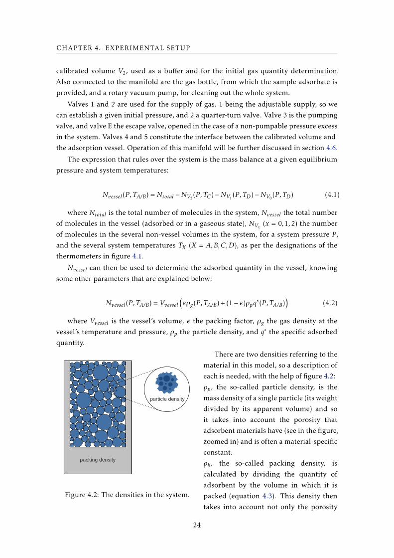
Figure 4.2: The densities in the system.
There are two densities referring to the
material in this model, so a description of
each is needed, with the help of figure 4.2:
ρp, the so-called particle density, is the
mass density of a single particle (its weight
divided by its apparent volume) and so
it takes into account the porosity that
adsorbent materials have (see in the figure,
zoomed in) and is often a material-specific
constant.
ρb, the so-called packing density, is
calculated by dividing the quantity of
adsorbent by the volume in which it is
packed (equation 4.3). This density then
takes into account not only the porosity
24
4.1. SYSTEM SUMMARY AND THE VOLUMETRIC METHOD
of the particle, but also the inter-particle space (figure 4.2) that an imperfect packing
inevitably has.
ρb =madsorbentVvessel
(4.3)
The packing factor, ε, tells us what fraction of the vessel corresponds to inter-particle
space, which is not filled by adsorbent. In essence, a perfect packing (ε = 0) would yield
a packing density equal to the particle density, as no interparticle space would exist:
ε = 1−ρbρp
(4.4)
We can now look at equation 4.2 and understand the two terms: the first, multiplied
by ε, refers to the portion of the vessel not filled by adsorbent, or the space between each
adsorbent particle, while the second, multiplied by 1 − ε, refers to the portion filled by
adsorbent, in which adsorption occurs at a quantity q∗.
The smaller this packing factor, the more adsorbent was packed into a container of a
given volume, which is attractive and very important in larger-scale projects due to
volume and budget restraints. There are, however, theoretical limits depending on the
distribution of particle sizes. Packing can be defined based on the number of distinct
particle sizes present, from equally sized particles (monomodal), two differing sizes
(bimodal), and so on (multimodal). An example of bimodal packing can be seen in
figure 4.1.
(a) (b)
Figure 4.3: Two illustrative, mathematical examples of a bimodal packing [32] a.
aReprinted with permission from J. Phys. Chem. C, Vol. 115, nr. 39, pp 19037–19040. Copyright 2011America Chemical Society.
For monomodal packing, a random packing of spheres uses approximately 64% of
space, giving us a packing factor ε of 36% [33]. This is the best packing one can expect
with a single particle size. For bimodal packing, ε goes down to 25%, and it gets lower and
lower for an increasing number of particle sizes (multimodal). Bimodal packing is often
25
CHAPTER 4. EXPERIMENTAL SETUP
the used method due to the fact that the quantity of adsorbent can simply be separated
in half – one half is crushed, being then reduced to a much smaller grain, and the other
half is unaffected, creating two different particle sizes – and because this simple process
increases the packing density by a significant quantity [34].
Rearranging equation 4.2 and using equation 4.1, we can obtain the adsorbed quantity
in terms of the system parameters:
q∗(P ,TA/B) =
Ntotal −NV2(P ,TC)−NV1
(P ,TD )−NV0(P ,TD )
Vvessel− ερg(P ,TA/B)
(1− ε)ρp(4.5)
We have then the defining equation for our system in equation 4.5 and can proceed
to the dimensioning, knowing all the involved quantities.
26
4.2. SYSTEM DIMENSIONING
4.2 System dimensioning
Dimensioning of the main components of the system — the adsorption vessel and the
calibrated volume — has to take into account the measurement method in use and the
extreme conditions when in operation.
The adsorption vessel and the calibrated volume must have dimensions such that the
system’s pressure variation over the course of a measurement is measurable by the
pressure sensors. Essentially, the initial quantity of gas in the calibrated volume has to
expand sufficiently into the adsorption vessel so that a significant pressure variation is
detected. This creates a compromise: the calibrated volume has to be larger than the
adsorption vessel and void volumes, but it cannot be so large that it requires an
impracticable quantity of gas for a substantial pressure variation to be read. Using
simulated data for neon adsorption on HKUST-1, calculated by J. P. Mota [21], an Excel
worksheet was made to gauge this compromise, calculating the pressure difference
between two extreme vessel temperatures and system pressures with the results
presented in table 4.1.
Table 4.1: Variations of pressure between two extreme vessel temperature and systempressure cases (130 K, 16 bar to 500 K, 100 bar).
Vvessel/cm3 Vcal/cm3 mads/g ∆P /bar
7.5 150 4 4.627.5 1500 4 0.46
Looking at table 4.1, the values of 7.5 cm3 and 150 cm3 were decided on: the
pressure variation of approximately 5 bar should be sufficient to carry out the
experiment, considering the sensitivity of the pressures sensors used.
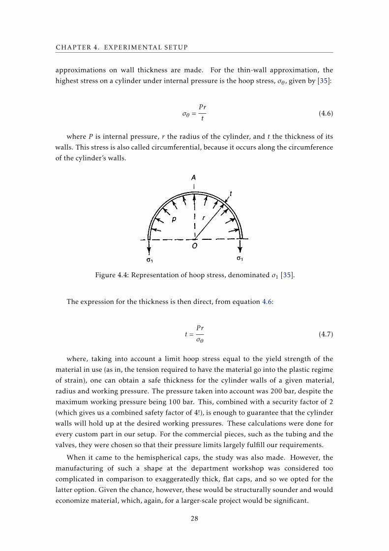
4.2.1 Wall thicknesses
The fact that the system will have to hold in pressures up to 100 bar makes it so that
some factors that would otherwise be irrelevant become critical — one in particular is the
thickness of the walls of the constituents: the adsorption vessel, the involved tubes and
the calibrated volume. Failure to accommodate such pressures can result in yield or even
fracture of the constituent materials, which could compromise the setup in several ways.
A strength study, implemented in an Excel worksheet, was made on the thickness of
walls for cylindrical pressure vessels with hemispherical caps — this shape was chosen
due to its structural resilience — applying the thin-wall and thick-wall approaches. The
thin-wall approximation assumes that the cylinder walls are infinitely thin in
comparison to the diameter, and so it is appliable when the thickness of the wall can be
considered sufficiently small in comparison to the diameter. Regardless, we concluded
from calculations that it was valid with an error of at most 10% (directly proportional to
the maximum allowed pressure) in comparison to the thick-wall assumption, where no
27
CHAPTER 4. EXPERIMENTAL SETUP
approximations on wall thickness are made. For the thin-wall approximation, the
highest stress on a cylinder under internal pressure is the hoop stress, σθ, given by [35]:
σθ =P r
t(4.6)
where P is internal pressure, r the radius of the cylinder, and t the thickness of its
walls. This stress is also called circumferential, because it occurs along the circumference
of the cylinder’s walls.
Figure 4.4: Representation of hoop stress, denominated σ1 [35].
The expression for the thickness is then direct, from equation 4.6:
t =P r
σθ(4.7)
where, taking into account a limit hoop stress equal to the yield strength of the
material in use (as in, the tension required to have the material go into the plastic regime
of strain), one can obtain a safe thickness for the cylinder walls of a given material,
radius and working pressure. The pressure taken into account was 200 bar, despite the
maximum working pressure being 100 bar. This, combined with a security factor of 2
(which gives us a combined safety factor of 4!), is enough to guarantee that the cylinder
walls will hold up at the desired working pressures. These calculations were done for
every custom part in our setup. For the commercial pieces, such as the tubing and the
valves, they were chosen so that their pressure limits largely fulfill our requirements.
When it came to the hemispherical caps, the study was also made. However, the
manufacturing of such a shape at the department workshop was considered too
complicated in comparison to exaggeratedly thick, flat caps, and so we opted for the
latter option. Given the chance, however, these would be structurally sounder and would
economize material, which, again, for a larger-scale project would be significant.
28
4.2. SYSTEM DIMENSIONING
4.2.2 Adsorption vessel
The two initial ideas were to either have disposable adsorption vessels or a reusable one
with a screw-on cap. The screw would then be tightened and filled with soft solder so
as to become leak-tight even at high pressures. The latter idea was opted for, and thus a
more detailed strength study was made for the screw in the cap, to determine the thread
parameters (figure 4.5) that allowed for large pressures.
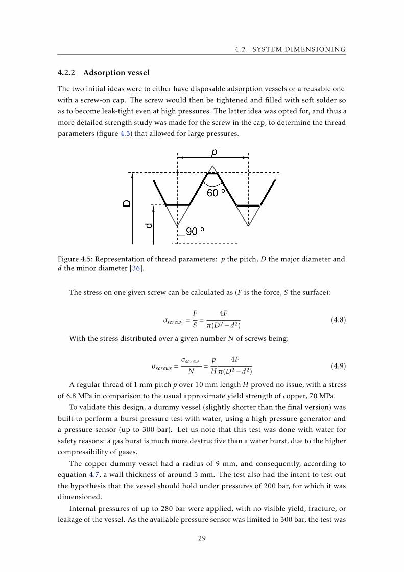
Figure 4.5: Representation of thread parameters: p the pitch, D the major diameter andd the minor diameter [36].
The stress on one given screw can be calculated as (F is the force, S the surface):
σscrew1=F
S=
4F
π(D2 − d2)(4.8)
With the stress distributed over a given number N of screws being:
σscrews =σscrew1
N=p
H
4F
π(D2 − d2)(4.9)
A regular thread of 1 mm pitch p over 10 mm lengthH proved no issue, with a stress
of 6.8 MPa in comparison to the usual approximate yield strength of copper, 70 MPa.
To validate this design, a dummy vessel (slightly shorter than the final version) was
built to perform a burst pressure test with water, using a high pressure generator and
a pressure sensor (up to 300 bar). Let us note that this test was done with water for
safety reasons: a gas burst is much more destructive than a water burst, due to the higher
compressibility of gases.
The copper dummy vessel had a radius of 9 mm, and consequently, according to
equation 4.7, a wall thickness of around 5 mm. The test also had the intent to test out
the hypothesis that the vessel should hold under pressures of 200 bar, for which it was
dimensioned.
Internal pressures of up to 280 bar were applied, with no visible yield, fracture, or
leakage of the vessel. As the available pressure sensor was limited to 300 bar, the test was
29
CHAPTER 4. EXPERIMENTAL SETUP
Figure 4.6: The dummy vessel built for pressure testing.
considered finished, with positive results: the vessel holds up in pressures at least almost
three times as high as the maximum working pressure of around 100 bar!
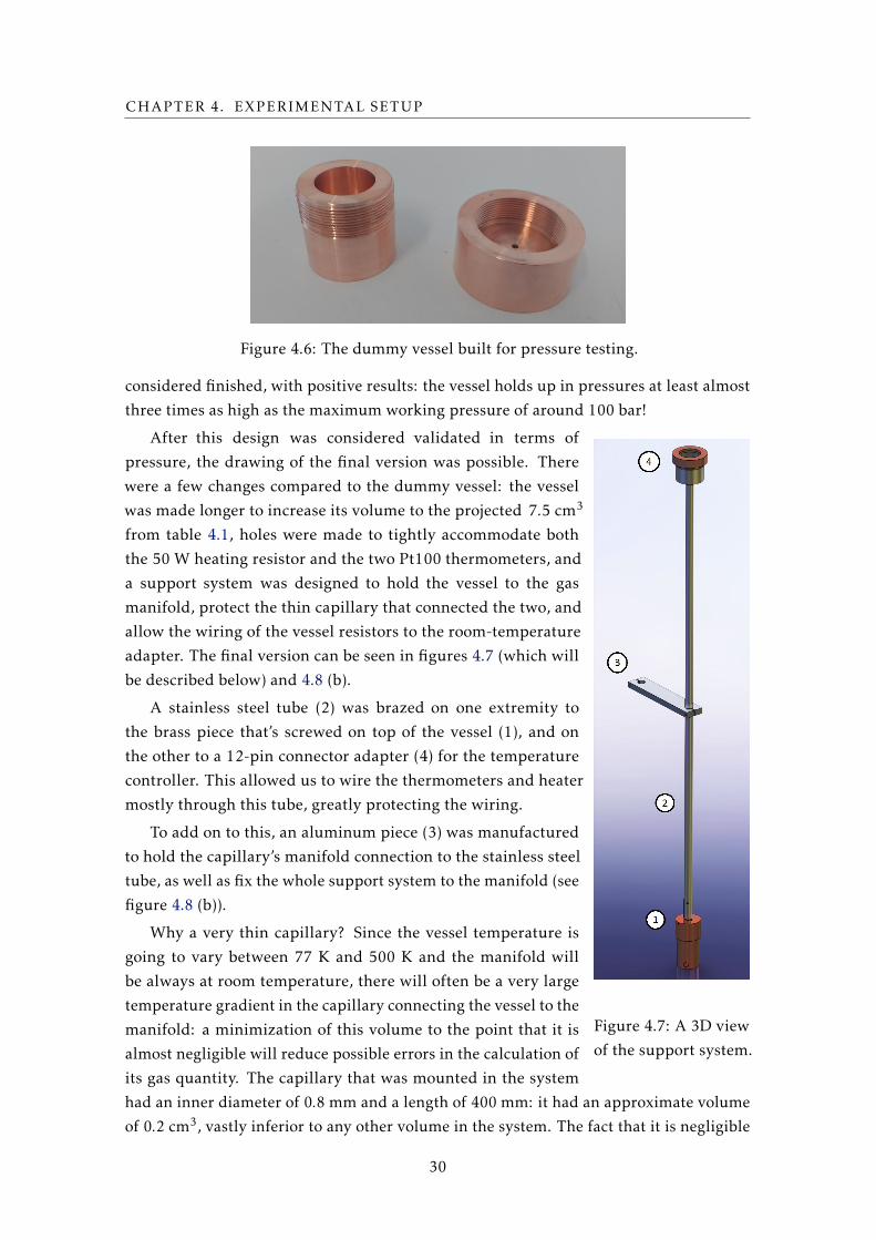
Figure 4.7: A 3D view
of the support system.
After this design was considered validated in terms of
pressure, the drawing of the final version was possible. There
were a few changes compared to the dummy vessel: the vessel
was made longer to increase its volume to the projected 7.5 cm3
from table 4.1, holes were made to tightly accommodate both
the 50 W heating resistor and the two Pt100 thermometers, and
a support system was designed to hold the vessel to the gas
manifold, protect the thin capillary that connected the two, and
allow the wiring of the vessel resistors to the room-temperature
adapter. The final version can be seen in figures 4.7 (which will
be described below) and 4.8 (b).
A stainless steel tube (2) was brazed on one extremity to
the brass piece that’s screwed on top of the vessel (1), and on
the other to a 12-pin connector adapter (4) for the temperature
controller. This allowed us to wire the thermometers and heater
mostly through this tube, greatly protecting the wiring.
To add on to this, an aluminum piece (3) was manufactured
to hold the capillary’s manifold connection to the stainless steel
tube, as well as fix the whole support system to the manifold (see
figure 4.8 (b)).
Why a very thin capillary? Since the vessel temperature is
going to vary between 77 K and 500 K and the manifold will
be always at room temperature, there will often be a very large
temperature gradient in the capillary connecting the vessel to the
manifold: a minimization of this volume to the point that it is
almost negligible will reduce possible errors in the calculation of
its gas quantity. The capillary that was mounted in the system
had an inner diameter of 0.8 mm and a length of 400 mm: it had an approximate volume
of 0.2 cm3, vastly inferior to any other volume in the system. The fact that it is negligible
30
4.2. SYSTEM DIMENSIONING
doesn’t necessarily mean that it doesn’t factor into calculations – an average temperature
between the vessel and the manifold was taken for this volume and considered in the
final calculations, despite having little effect in the results.
(a) (b)
Figure 4.8: In (a), the final version of the vessel. Note the smaller holes for Pt100thermometers. In (b), the support system mounted on the manifold, to be comparedto figure 4.7.
The volume of this final vessel (figure 4.8, (a)) was then measured to confirm our
initial projection. The measurements were done by weighing the vessel, both completely
empty and completely filled with distilled water, and taking the difference as the mass
of water inside. This can then directly be converted to the volume of water inside. The
drawing had a volume of 7.634 cm3, while the measurement yielded 7.63 cm3, leading
us then to conclude that we could use this value as a constant for the rest of the work to
be carried out and that we had been able to determine a very important volume for the
proper functioning of our method.
31
CHAPTER 4. EXPERIMENTAL SETUP
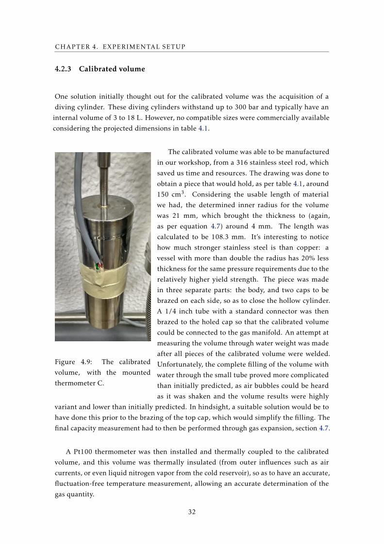
4.2.3 Calibrated volume
One solution initially thought out for the calibrated volume was the acquisition of a
diving cylinder. These diving cylinders withstand up to 300 bar and typically have an
internal volume of 3 to 18 L. However, no compatible sizes were commercially available
considering the projected dimensions in table 4.1.
Figure 4.9: The calibrated
volume, with the mounted
thermometer C.
The calibrated volume was able to be manufactured
in our workshop, from a 316 stainless steel rod, which
saved us time and resources. The drawing was done to
obtain a piece that would hold, as per table 4.1, around
150 cm3. Considering the usable length of material
we had, the determined inner radius for the volume
was 21 mm, which brought the thickness to (again,
as per equation 4.7) around 4 mm. The length was
calculated to be 108.3 mm. It’s interesting to notice
how much stronger stainless steel is than copper: a
vessel with more than double the radius has 20% less
thickness for the same pressure requirements due to the
relatively higher yield strength. The piece was made
in three separate parts: the body, and two caps to be
brazed on each side, so as to close the hollow cylinder.
A 1/4 inch tube with a standard connector was then
brazed to the holed cap so that the calibrated volume
could be connected to the gas manifold. An attempt at
measuring the volume through water weight was made
after all pieces of the calibrated volume were welded.
Unfortunately, the complete filling of the volume with
water through the small tube proved more complicated
than initially predicted, as air bubbles could be heard
as it was shaken and the volume results were highly
variant and lower than initially predicted. In hindsight, a suitable solution would be to
have done this prior to the brazing of the top cap, which would simplify the filling. The
final capacity measurement had to then be performed through gas expansion, section 4.7.
A Pt100 thermometer was then installed and thermally coupled to the calibrated
volume, and this volume was thermally insulated (from outer influences such as air
currents, or even liquid nitrogen vapor from the cold reservoir), so as to have an accurate,
fluctuation-free temperature measurement, allowing an accurate determination of the
gas quantity.
32
4.3. VESSEL FILLING AND PREPARATION
4.3 Vessel filling and preparation
For the adsorption vessel to be ready for the introduction of the sample, mounting of
the resistors and soldering of the cap (a process which was repeated several times over
the course of this work), it must be thoroughly clean. This was done initially by hand
to remove any obvious moisture and finalized with an ultrasonic bath, set to 10 minutes
using acetone. This cleaning procedure is important for the inner part of the vessel, which
will be in contact with the sample, but also for the outer threaded part, in order to allow
a good wetting of the screw to be soldered.
Figure 4.10: The
vessel, post-filling.
Filling the vessel with HKUST-1 has to be a careful process,
as the material is toxic and ours had a very small grain size
of 16 µm (see table 2.1), meaning it behaved almost like very
light dust. Thus, protective equipment such as glasses, gloves
and a dust mask are advised, as well as careful handling. The
material doesn’t seem to adhere at all to paper, which makes
it a suitable base to carry out the filling. The greatest possible
amount of adsorbent has to be put into the vessel, which requires
mechanical vibrations by hand on the vessel as the filling is done,
to force the sample to fully settle (as best as possible) in the free
space beneath it. Further compression was made with a metal
piece to attempt a greater degree of packing. The vessel was
weighed before and after this process to determine the mass of
sample that had been packed into it.
Figure 4.11: Vestigial amounts
of HKUST-1 outside the vessel.
To prevent the sample from leaving the vessel as
pumping or fast gas discharges occur, some type of filter
had to be applied. The choice fell on a stainless steel
grid with 25 µm holes as well as a small quantity of glass
wool in the tube exiting the vessel’s cap. This quantity of
glass wool is crucial, as an initial experiment with only
the aluminum grid had us discover that the sample left
the vessel quite easily (figure 4.11, in light blue). This
forced us to clean out the system, as we had pumped a
small quantity of sample.
The cap is then tightly screwed on and the complete
vessel exposed to a pre-activation period in order to
remove unwanted moisture from the sample. After
staying overnight at 80 ºC in a low vacuum, the muffle
oven is filled with nitrogen to prevent adsorptions of
other species present in air. After this process, the vessel
is weighed to confirm the quantity inside (small variations of mass might occur in
activation, figure 3.2). The vessel’s screw is then ready to be filled with solder.
33
CHAPTER 4. EXPERIMENTAL SETUP
(a)
0
50
100
150
200
250
300
0 10 20 30 40 50 60Te
mp
erat
ure
/ o
C
Time / min
(b)
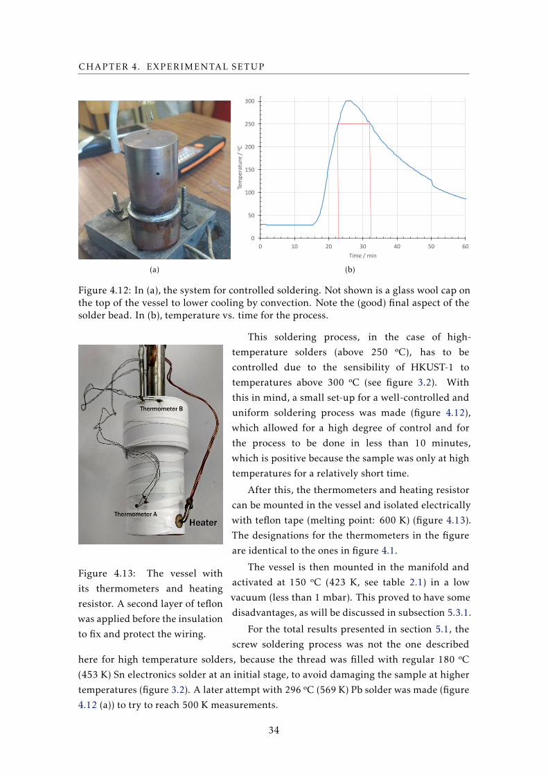
Figure 4.12: In (a), the system for controlled soldering. Not shown is a glass wool cap onthe top of the vessel to lower cooling by convection. Note the (good) final aspect of thesolder bead. In (b), temperature vs. time for the process.
Figure 4.13: The vessel with
its thermometers and heating
resistor. A second layer of teflon
was applied before the insulation
to fix and protect the wiring.
This soldering process, in the case of high-
temperature solders (above 250 ºC), has to be
controlled due to the sensibility of HKUST-1 to
temperatures above 300 ºC (see figure 3.2). With
this in mind, a small set-up for a well-controlled and
uniform soldering process was made (figure 4.12),
which allowed for a high degree of control and for
the process to be done in less than 10 minutes,
which is positive because the sample was only at high
temperatures for a relatively short time.
After this, the thermometers and heating resistor
can be mounted in the vessel and isolated electrically
with teflon tape (melting point: 600 K) (figure 4.13).
The designations for the thermometers in the figure
are identical to the ones in figure 4.1.
The vessel is then mounted in the manifold and
activated at 150 ºC (423 K, see table 2.1) in a low
vacuum (less than 1 mbar). This proved to have some
disadvantages, as will be discussed in subsection 5.3.1.
For the total results presented in section 5.1, the
screw soldering process was not the one described
here for high temperature solders, because the thread was filled with regular 180 ºC
(453 K) Sn electronics solder at an initial stage, to avoid damaging the sample at higher
temperatures (figure 3.2). A later attempt with 296 ºC (569 K) Pb solder was made (figure
4.12 (a)) to try to reach 500 K measurements.
34
4.4. LABVIEWTM
INTERFACE
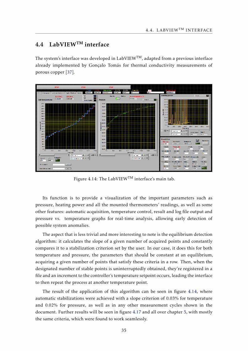
4.4 LabVIEWTM interface
The system’s interface was developed in LabVIEWTM, adapted from a previous interface
already implemented by Gonçalo Tomás for thermal conductivity measurements of
porous copper [37].
Figure 4.14: The LabVIEWTM interface’s main tab.
Its function is to provide a visualization of the important parameters such as
pressure, heating power and all the mounted thermometers’ readings, as well as some
other features: automatic acquisition, temperature control, result and log file output and
pressure vs. temperature graphs for real-time analysis, allowing early detection of
possible system anomalies.
The aspect that is less trivial and more interesting to note is the equilibrium detection
algorithm: it calculates the slope of a given number of acquired points and constantly
compares it to a stabilization criterion set by the user. In our case, it does this for both
temperature and pressure, the parameters that should be constant at an equilibrium,
acquiring a given number of points that satisfy these criteria in a row. Then, when the
designated number of stable points is uninterruptedly obtained, they’re registered in a
file and an increment to the controller’s temperature setpoint occurs, leading the interface
to then repeat the process at another temperature point.
The result of the application of this algorithm can be seen in figure 4.14, where
automatic stabilizations were achieved with a slope criterion of 0.03% for temperature
and 0.02% for pressure, as well as in any other measurement cycles shown in the
document. Further results will be seen in figure 4.17 and all over chapter 5, with mostly
the same criteria, which were found to work seamlessly.
35
CHAPTER 4. EXPERIMENTAL SETUP
4.5 Cooling and heating system
As already mentioned in subsection 4.2.2, two Pt100 thermometers and a 50 W heating
resistor make up the sensing and heating part of the developed cooling and heating
system, respectively. The used temperature controller was a LakeShore 336 model,
interfaced with the LabVIEWTM program introduced in the previous section.
Simply cooling is a relatively simple task, as surrounding the vessel with liquid
nitrogen will very quickly thermalize it to around 77 K. Accurately controlling the
temperature through heating against a liquid nitrogen reservoir from 77 K to 500 K is,
however, a completely different challenge. The vessel has to be insulated from the cold
source to the point where its temperature can be raised, but not too insulated so that it
allows enough cooling power for temperature control to be possible.
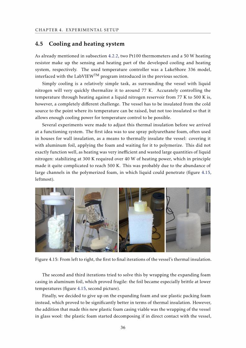
Several experiments were made to adjust this thermal insulation before we arrived
at a functioning system. The first idea was to use spray polyurethane foam, often used
in houses for wall insulation, as a means to thermally insulate the vessel: covering it
with aluminum foil, applying the foam and waiting for it to polymerize. This did not
exactly function well, as heating was very inefficient and wasted large quantities of liquid
nitrogen: stabilizing at 300 K required over 40 W of heating power, which in principle
made it quite complicated to reach 500 K. This was probably due to the abundance of
large channels in the polymerized foam, in which liquid could penetrate (figure 4.15,
leftmost).
Figure 4.15: From left to right, the first to final iterations of the vessel’s thermal insulation.
The second and third iterations tried to solve this by wrapping the expanding foam
casing in aluminum foil, which proved fragile: the foil became especially brittle at lower
temperatures (figure 4.15, second picture).
Finally, we decided to give up on the expanding foam and use plastic packing foam
instead, which proved to be significantly better in terms of thermal insulation. However,
the addition that made this new plastic foam casing viable was the wrapping of the vessel
in glass wool: the plastic foam started decomposing if in direct contact with the vessel,
36
4.5. COOLING AND HEATING SYSTEM
when high temperatures were applied. Glass wool is an insulating material made from
fibres of glass and has a texture similar to wool, which makes it highly malleable and
adaptable to different shapes. This was enough to properly insulate the vessel but still
allow it to cool down to our reservoir’s 77 K. A custom vessel-sized casing was then
carved, with some help from the workshop, to house the glass wool-wrapped vessel for
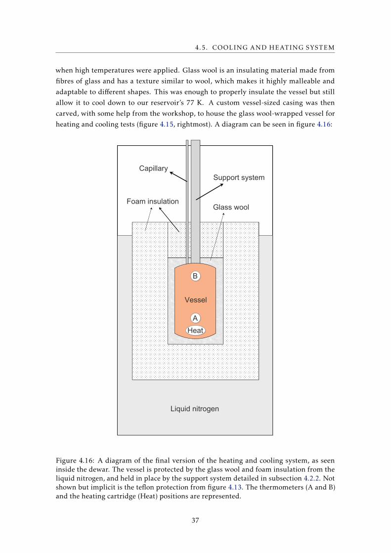
heating and cooling tests (figure 4.15, rightmost). A diagram can be seen in figure 4.16:
Vessel
Support systemCapillary
Liquid nitrogen
Glass woolFoam insulation
B
A
Heat
Figure 4.16: A diagram of the final version of the heating and cooling system, as seeninside the dewar. The vessel is protected by the glass wool and foam insulation from theliquid nitrogen, and held in place by the support system detailed in subsection 4.2.2. Notshown but implicit is the teflon protection from figure 4.13. The thermometers (A and B)and the heating cartridge (Heat) positions are represented.
37
CHAPTER 4. EXPERIMENTAL SETUP
These tests consisted of programming the temperature controller’s PID
(proportional-integral-differential) parameters. These parameters are coefficients in the
PID mechanism, which consists of the calculation of the difference between a desired
setpoint and a measured process variable (in our case, the temperature), denominated
error value. It then attempts to minimize this difference by adjusting a control variable
(in our case, the heating power). The name of this mechanism comes from the expression
that rules over it:
u(t) = P e(t) + I∫ t
0e(τ)dτ +D
de(t)dt
(4.10)
where u(t) is the control variable value, e the error value, P the proportional coefficient,
I the integral coefficient, and D the differential coefficient. These three coefficients were
determined by trial-and-error, so that the stabilization occurred within a reasonable time-
frame. Over such a large temperature range (77 K to 500 K), it’s often not enough to
define a single group of these three values due to the large variation of thermal properties
in this temperature range: in our case, 3 different regions had to be defined and so a total
of 9 coefficients had to be determined in a trial-and-error process. More practical results
can be observed in the next page, figure 4.17. Stabilization in temperature was able to be
done to the third decimal place given enough time!
Considering the temperature target (500 K or 223 ºC), the solder used in the sensors
and heater could not be a typical Sn solder (180 ºC fusion point). Therefore, these
components were welded with a Pb solder (93%), containing also small amounts of Sn
(5%) and Ag (2%), with a fusion point of 296 ºC, which is widely above our temperature
limit and so it doesn’t risk any desoldering.
Cooling down the vessel usually took around 20 minutes, whereas fulfilling a full
heating cycle from 77 K to 500 K took the system as long as 4 hours, depending on the
amount of setpoints used. This is appreciable, since, concerning the volumetric method, a
handful of cycles at different pressures are enough to trace out isotherms over a relatively
wide range, which was the final goal of this work.
38
4.5. COOLING AND HEATING SYSTEM
0
5
10
15
20
25
30
35
40
45
50
75
80
85
90
95
100
105
110
115
120
125
20 40 60 80 100 120
Po
we
r /
W
Tem
pe
ratu
re /
K
Time / min
Temperature
Power
LN2
(a)
0
5
10
15
20
25
30
100
150
200
250
300
350
400
450
500
50 100 150 200 250
Pow
er /
W
Tem
per
atu
re /
K
Time / min
Temperature
Power
(b)
Figure 4.17: An example of temperature stabilizations in the whole temperature range,lower in (a) and higher in (b), with a temperature slope criterion of 0.03%. Notice theheating peaks and following stabilization in temperature. The vessel was empty for thesetests.
39
CHAPTER 4. EXPERIMENTAL SETUP
4.6 Experimental procedure
Two specific variations of the volumetric method were initially discussed to perform the
experiments, and they will be illustrated in the pages that follow.
Figure 4.18: The manifold, fully wall mounted. Compare to figure 4.1 and note thesupport system described in subsection 4.2.2, figure 4.7, on the left after valve 5, as wellas the insulation for the calibrated volume described in 4.2.3, after valve 4 in the bottom.
The first discussed procedure, A, is the most similar to the volumetric method
described in the state of the art. A measurement should be made through these steps:
1. Cleaning phase: with the gas supply closed (valves 1 and 2) and the rest completely
open, the system is pumped to a low vacuum (less than 1 mbar).
2. Filling of the calibrated volume: closing valves 3 and 5 and opening valve 1, open
valve 2 to a given initial pressure Pi . Measuring the pressure and temperature of
the calibrated volume, the total amount of gas in the calibrated volume at that time,
and in total for the whole system after step 3, can be determined. Close valve 4 and
pump the system, except the calibrated volume.
3. Expansion to vessel and measurement: expansion by opening valves 4 and 5. The
vessel can then be set to a temperature and the pressure read over a given period of
time, giving us access to the adsorbed quantity of gas dependent on pressure for a
given vessel temperature.
4. Stabilized heating cycle: to obtain a set of various q∗ points, sweep vessel
temperature setpoints from 77 K to 500 K (see, for instance, figure 4.17). This gives
access to adsorption curves, quantity versus temperature and pressure.
A variation of this first procedure, B, arose for the emulation of an actual adsorption
compressor, capable of very large pressure differences. The calibrated volume is removed
40
4.6. EXPERIMENTAL PROCEDURE
(i.e., valve 4 permanently closed), making V0 and V1 the actual “calibrated volume”.
This setup is the most possibly similar to the first phase (pre-heating) of an adsorption
compressor’s functioning cycle.
The procedure is essentially identical in terms of setup, excluding valve 4 and the
calibrated volume from procedure A. Instead of carrying out an expansion, the gas
resides in only V0, V1 and the adsorption vessel. We will later be able to observe that,
since the room temperature volume is much smaller, adsorption and desorption will lead
to considerably larger pressure variations.
Procedure A was the most used one: the big disadvantage in procedure B is caused by
the absence of the calibrated volume as a buffer. The capillary’s volume becomes much
more significant in comparison to the total system volume, which means an error in its
temperature (which is inevitable, due to a very large gradient along it) becomes an actual
issue. Through the same rationale, an error in the determination of V1 is now also much
more significant in a relative way, which also induces greater, unpredictable errors in the
results. A comparison of results obtained with both these procedures will be made in
chapter 5 and the conclusions will be similar.
0
10
20
30
40
50
60
70
80
90
100
0 20 40 60 80 100 120 140
Pre
ssu
re /
bar
Time / min
Gas bottle closed
Gas bottle open
Adsorption saturation at 50 bar, 77 K
Opening calibrated volume (60 bar)
Heating to 300 K(desorption)
Closing calibrated volume (80 bar)
Cooling to 77 K (adsorption)
Figure 4.19: The method to go beyond the bottle’s pressure.
A procedure for filling the calibrated volume arose because the pressure in the neon
bottle was about 60 bar, and its pressure reducer was limited to 70 bar. To circumvent
these limitations, the vessel filled with HKUST-1 was used as a thermal compressor,
through heating cycles between 77 K and 300 K, in order to fill the calibrated volume
with a desired pressure above our bottle and reducer limits. In short, a cycle of adsorbent
saturation (through cooling) and neon desorption (through heating) raises the pressure
in the calibrated volume. The different steps are detailed in figure 4.19.
41
CHAPTER 4. EXPERIMENTAL SETUP
4.7 Determination of system volumes
The determination of the main volumes in the system was, as already detailed in section
4.1, the most critical part to properly interpreting the obtained data.
Vessel
DewarCalibrated
volumeGas bottle
Pressure sensor 2
Pressure sensor 1
Vvessel V2
25 1V1
V0
Vacuum pump
E
3
4
V1manifold
V1capillary
12.63 cm3
150.26 cm3
6.15 cm3
0.20 cm3
7.63 cm3
Figure 4.20: The volume designations in the system and their capacity, determined asexplained in the text below.
There are several ways to achieve an accurate determination of the volume capacity.
Perhaps the most simple is a gas expansion from a calibrated volume to the volume we
wish to determine. Through two pressure measurements, one can accurately and quickly
determine the total volume and thus the variation in volume, correspondent to the value
we want to find out. Assuming a closed system and constant temperature:
Ni =Nf → PiVc = Pf (Vc +V?)→ V? =
PiPf − 1
Vc (4.11)
where Vc is a calibrated volume, V? the volume we wish to determine, and Pi and Pfthe pressures values before and after the expansion, respectively.
However, when one does not have a well-calibrated volume available to do this simple
process, another possibility is to use a known volume variation to obtain a well-calibrated
volume in a system. To this effect, an adjustable calibrated volume was borrowed from
the METROVAC laboratory at FCT-UNL. From its measurements (3.1 cm diameter, 0.175
cm screw pitch), we could calculate the volume variation per turn of the adjustable wheel.
In this case, the calibrated variable is not the volume, but the variation in volume when
the adjustable wheel is turned:
Vturn = π
3.1
2
2
0.175 = 1.245cm3 (4.12)
42
4.7. DETERMINATION OF SYSTEM VOLUMES
V0
Vc
ΔV
Ajustable wheel
Valve
Figure 4.21: A
diagram of the
method for V0.
The volume most easily determined through this method, due
to accessibility, was V0, the central volume in the manifold. It’s
then simple to apply equation 4.11 but for a variation in volume
∆V , with Vc the calibrated volume’s initial capacity, which is also
unknown:
Pi(Vc +V0) = Pf (Vc +V0 +∆V )→ Vc +V0 =
PfPi − Pf
∆V (4.13)
This leaves us with knowledge of the volume we want to know,
V0, added to the initial calibrated volume that we in principle do
not know, Vc. We can, however, with current knowledge of the
pressure, close the calibrated volume’s valve and pump V0, do yet
another expansion, now from the calibrated volume to the volume
to be determined. Vc is then given by:
Pi(Vc+∆V ) = Pf (Vc+V0 +∆V )→ Vc =PfPi
(Vc+V0 +∆V )−∆V (4.14)
Having determined the initial calibrated volume Vc, from
equation 4.14 and having knowledge of the total initial volume
Vc+V0 from equation 4.13, we can subtract one from the other and
obtain V0. This was done through both compression and expansion
of the calibrated volume over 20 times to accumulate statistics,
giving us a very well-defined volume.
From here, V0 could be used as the calibrated volume for
expansions carried out into the other volumes to be determined,
by equation 4.11: V1 and V2 were both determined through this
method. The obtained values after this volume determination are indicated in figure 4.20.
These values were considered constant for the rest of the work done, as there was a great
deal of confidence in V0: the volumes determined from expansions starting in it should
then be correct. This is due to the great amount of measurements done with the adjustable
calibrated volume and to the relative precision of a standard gas expansion: the process
is instant and the only significant error to be taken into account is of a pressure reading.
The resolution of the pressure sensor (0.002% of the 10 bar absolute full scale, which is
0.2 mbar), which had been zeroed in a vacuum, was quite good, which leaves us confident
in the pressure (and consequently volume) measurements carried out.
It’s also worth mentioning that extensive leak testing was performed in this initial
phase, so as to minimize any possible losses of gas, which would greatly affect both the
method and our initial calculation of V0, as these are relatively lengthy processes. This
length could have been significantly reduced if a careful measurement of the calibrated
volume’s capacity had been done before the caps were welded.
43
CHAPTER 4. EXPERIMENTAL SETUP
4.8 Empty-vessel tests
With the intention to confirm the volumes determined in the previous section, some tests
with helium as a working gas were made, with no sample inside the vessel.
The idea was to use the mass balance equation 4.1 to, after knowing the total quantity
of helium in the system, calculate the portion in the adsorption vessel. Comparing it
with the real quantity present at the measured temperature and pressure through NIST’s
REFPROP [38], we can then deduce the error that is being made through this mass balance
calculation. Moreover, these tests were used to test silicone paste as a leak-tight screw
seal for high pressures and low temperatures, instead of soft solder.
-10
-8
-6
-4
-2
0
2
4
6
8
10
150 200 250 300 350 400 450 500 550
% e
rro
r
Temperature (K)
(a)
-10
-8
-6
-4
-2
0
2
4
6
8
10
150 200 250 300 350 400 450 500 550
% e
rro
r
Temperature / K
(b)
Figure 4.22: The relative error of ideal vs. real (REFPROP) gas quantity in the vessel forseveral heating cycles done at circa 2 bar for the first, (a), and second, (b), silicon tries.
44
4.8. EMPTY-VESSEL TESTS
In essence, the relative error represented in figure 4.22 is:
ρvessel =NvesselVvessel
=Ntotal −NV0
−NV1−NV2
Vvessel(4.15)
As we can observe in figure 4.22, the best results were all mostly in range of 2%
error for the first try and 4% error for the second, which is a decent mark for volumetric
measurements. Some other results were taken, including at higher pressures, but the
ones presented above exhibited the best reproducibility. Other results went up to 5%
error only in the higher temperature range (400 K to 500 K), which proved difficult to
understand and solve.
This motivated us to not to take many conclusions from these tests due to not
understanding these variations.
Figure 4.23: The silicone
excess in the second round.
For these tests, some experiments on sealing the screw
with high temperature resistant silicone were made. Two
tries were made: for the second try, some irregular results
(not presented here) led us to conclude that we had
exaggerated in the used quantity and thus reduced the
vessel volume through an excess of silicone on the inside,
which proved true as we opened it up (figure 4.23). This
might explain the bigger maximum error in the second
try. We found that the silicone repeatedly leaked above 5
bar internal pressure, which restrained our empty-vessel
studies to low pressures. This motivated us to move on to
testing on a sample and discard the possibility of silicone
for the thread filling. Regarding the minimum tested
temperature of 200 K: we weren’t sure that the silicone
would behave properly at 77 K and therefore, since we
instantly stopped after realizing it wasn’t suited for high
pressures, we did not perform measurements below 200 K.
As such, we considered that the system was ready to obtain adsorption results on
HKUST-1. In the next chapter we will look back in a critical way, exposing, analyzing and
discussing these results and what possible factors from our dimensioning and preparation
detailed in this chapter 4 could impact them positively or negatively.
45
Chapter
5Results and analysis
5.1 Neon on HKUST-1 adsorption isotherms
The results were treated using an Excel worksheet programmed for automatic result
analysis and tracing of isotherms, using equation 4.5. For any and all result treatment
done in this chapter, the real (as opposed to ideal) gas quantities at given temperatures
and pressures were given by NIST’s REFPROP [38], to avoid unnecessary errors, even
if minimal in certain ranges. Initially, the treatment had been done with the ideal gas
equation but at higher temperatures and pressures the compressibility factor Z of neon
differs by up to 4%, which is enough to induce significant errors in adsorption quantity.
An example will be given in subsection 5.3.2.
Another source of errors, since we’re working in a quite large temperature and
pressure range, is the expansion and contraction of the vessel due to temperature and/or
pressure. The variation of the vessel’s volume due to variation in its temperature was
then accounted for, using copper dilation data from NIST [39]. Between 77 K and 500 K
the vessel volume varies by around 0.15 cm3, which can induce an error of up to 2% in
the adsorption quantity. Calculations on the volume variation due to pressure were
made, but the contribution was insignificant. A table summarizing the percentual
influence of errors in volume determination, mass determination, the real gas correction,
and the thermal expansion correction, will be presented in subsection 5.3.1.
An aspect worth revisiting is the packing factor ε (section 4.1), and how much
adsorbent we were able to pack into our adsorption vessel, for the reasons already
explained. Keeping in mind that the distribution of our commercial HKUST-1 was
monomodal (16 µm particle size, table 2.1), the best ε we could realistically achieve was
36%, which means 64% of the vessel is filled by HKUST-1. As such, we made several
packing attempts in which we attempted to pack the most possible HKUST-1 into our
47
CHAPTER 5. RESULTS AND ANALYSIS
vessel, as per the procedure in section 4.3. For the total results presented in this section,
ε was 45%, corresponding to an adsorbent mass of 3.955 g. Our best result, however, was
a packing factor ε of 42%, for the last, short experiment presented in the next section,
which corresponded to an adsorbent mass of 4.165 g.
For a single measurement session, following procedure A outlined in 4.6, the
temperature was varied from 77 K to 400 K, obtaining the results in figure 5.1 (b).
20
22
24
26
28
30
32
34
50
100
150
200
250
300
350
400
0 50 100 150 200 250 300 350 400 450 500
Pre
ssu
re /
bar
Ve
sse
l te
mp
era
ture
/ K
Time / min
Vessel temperature
Pressure
(a)
1000
20
22
24
26
28
30
32
34
0
2
4
6
8
10
12
14
16
18
20
70 120 170 220 270 320 370 420
Pre
ssu
re /
bar
q*
/ m
mo
l/g
Vessel temperature / K
Adsorbed quantity
Pressure
(b)
Figure 5.1: System parameters and results for a session. In (a), variations of pressure andvessel temperature. In (b), adsorbed quantity and pressure vs. vessel temperature.
48
5.1. NEON ON HKUST-1 ADSORPTION ISOTHERMS
In this figure, for an initial calibrated volume filling pressure of around 38 bar, it’s
interesting to notice how the system pressure follows the vessel temperature very strongly
due to adsorption. We can further observe the effect in the pressure: from 77 K to 300 K
and for a total system volume of around 175 cm3, there’s a compression of 12 bar, from
20 bar to 32 bar.
Seven other sessions, similar to the one presented above but at different initial
calibrated volume filling pressures (from 5 bar up to 76 bar), were performed to cover a
wide pressure range.
To trace out an isothermic curve (i. e. the quantity of adsorbed gas vs. pressure at a
fixed temperature), we must always use the same temperature setpoints for the automatic
control (see sections 4.4 and 4.5) in different measurement sessions, which will then be
the temperatures corresponding to our different isotherms. The intervals decided on
were, in short: after the initial setpoint of 77 K (thermalized with liquid nitrogen), from
80 K to 100 K in 5 K intervals, from 100 K to 200 K in 10 K intervals, and from 200 K on
in 20 K intervals.
With this in consideration, the total results taken are presented in the next two pages,
in the form of isotherms (figures 5.2 and 5.3).
49
0 5
10
15
20
25
01
02
03
04
05
06
07
0
q* / mmol/g
Pressu
re / bar
T = 7
7 K
T = 8
0 K
T = 8
5 K
T = 9
0 K
T = 9
5 K
T = 1
00
K
T = 1
10
K
T = 1
20
K
T = 1
30
K
T = 1
40
K
T = 1
50
K
T = 1
60
K
T = 1
70
K
T = 1
80
K
T = 1
90
K
T = 2
00
K
T = 2
20
K
T = 2
40
K
T = 2
60
K
T = 2
80
K
T = 3
00
K
T = 3
20
K
T = 3
40
K
T = 3
60
K
T = 3
80
K
T = 4
00
K
Figure
5.2:The
totaladsorp
tionisotherm
su
pto
400K
.Ou
tlinedis
theset
ofresu
ltsfrom
figu
re5.1
(b).
50
1.4
00
1.6
00
1.8
00
2.0
00
Q* / MMOL/G
T =
77
KT
= 8
0 K
T =
85
KT
= 9
0 K
T =
95
KT
= 1
00
KT
= 1
10
KT
= 1
20
KT
= 1
30
KT
= 1
40
KT
= 1
50
KT
= 1
60
KT
= 1
70
KT
= 1
80
KT
= 1
90
K
0
0.51
1.52
2.53
3.54
4.55
01
02
03
04
05
06
07
0
q* / mmol/g
Pre
ssu
re /
bar
T =
77
K
T =
80
K
T =
85
K
T =
90
K
T =
95
K
T =
10
0 K
T =
11
0 K
T =
12
0 K
T =
13
0 K
T =
14
0 K
T =
15
0 K
T =
16
0 K
T =
17
0 K
T =
18
0 K
T =
19
0 K
T =
20
0 K
T =
22
0 K
T =
24
0 K
T =
26
0 K
T =
28
0 K
T =
30
0 K
T =
32
0 K
T =
34
0 K
T =
36
0 K
T =
38
0 K
T =
40
0 K
Figu
re5.
3:T
hehi
gher
tem
per
atu
reis
othe
rms
not
dis
cern
ible
infi
gure
5.2.
51
CHAPTER 5. RESULTS AND ANALYSIS
Firstly, the total results exhibit the expected tendencies (see figure 2.2 for comparison):
at constant temperature T , the adsorbed quantity q∗ increases as the pressure P increases.
At low P , q∗ is proportional to P (the Henry’s Law isotherm). At high T , q∗ is essentially
linear over the whole pressure range, as was expected.
During this process, we trialed the second experimental procedure, B, detailed in
4.6, to verify its validity and confirm our already taken results, as seen in figure 5.4.
First of all, the pressure variation over a single measurement session is, due to the much
smaller volume being compressed, much larger compared to our normal measurements:
the variation of around 30 bar (corresponding to a factor higher than 7, from 4 bar to
35 bar) in around 30 cm3 with a few grams of adsorbent material suggests it is a very
efficient compressor.
0
1
2
3
4
5
6
7
8
9
10
0 5 10 15 20 25 30 35 40
q*
/ m
mo
l/g
Pressure / bar
T = 77 K
T = 80 K
T = 85 K
T = 90 K
T = 95 K
T = 100 K
T = 120 K
T = 140 K
T = 160 K
T = 180 K
T = 200 K
T = 240 K
T = 280 K
T = 320 K
Figure 5.4: The points obtained using procedure B (crosses) overlapped with the totalresults from figure 5.2.
As can be seen, the points overlap with the tendency exhibited by the results in the
first method and start to drift away for larger temperatures. As we had already discussed
in section 4.6, this might imply an error, even if minimal, in one of the volumes of the
system, V0 or V1, as this method is much more sensitive in that regard due to a smaller
total system volume (about 15 times smaller): a 0.5 cm3 variation induces errors up to
20% at higher temperatures, where the results drift away. Another possible explanation
for this slight upwards drift is the existence of a leak, which would be more noticeable in
pressure as time went on when compared to a much larger volume. A leak would lower
the pressure of the system, which, as it’s assumed we conserve the total quantity of neon,
makes it seem like more gas is adsorbed. This explanation was discarded after extensive
leak testing.
As explained in section 4.3, the results presented in figures 5.2, 5.3 and 5.4 were
52
5.2. 400 K TO 500 K RESULTS
only taken up to 400 K, due to an initial concern in not damaging the sample. This
solder held up until the experiments above 400 K and 70 bar, where we started to have
repetitive leaks in the filling, which motivated us to move on to the higher-temperature,
more resistant Pb-based solder.
5.2 400 K to 500 K results
The filling and sealing of the vessel was then made with the 296 ºC Pb solder and pressure-
tested at room temperature up to 40 bar for leaks, with positive results. The question was
whether the sample had been damaged by the soldering temperature or not. Thus, we
performed measurements to evaluate the sample’s damage, which yielded the results in
figure 5.5.
0
5
10
15
20
25
20 30 40 50 60 70 80
q*
/ m
mo
l/g
Pressure / bar
T = 77 K
T = 100 K
T = 110 K
T = 120 K
T = 130 K
T = 140 K
T = 150 K
T = 160 K
T = 170 K
T = 180 K
T = 190 K
T = 200 K
T = 220 K
T = 240 K
T = 260 K
T = 280 K
T = 300 K
T = 320 K
Figure 5.5: In the dashed ellipse, the points taken after the 296 ºC soldering, with theprevious results.
As we can see, the sample most definitely lost adsorptive capabilities, and so we
could conclude that it was damaged by the high temperature applied when soldering. A
thermogravimetric analysis made by LATPE showed that decomposition of the sample
can happen, in just a few minutes, anywhere above 275 ºC, compared to the 300 ºC
suggested in figure 3.2. It’s likely that our sample suffered such a degradation during the
soldering process, which is a bit more complicated at these higher temperatures (due to
the considerable heating power required).
Moreover, at around 340 K, with a pressure of 76 bar in the vessel, the screw filling
opened a very small leak and consequently experiments had to be stopped. Regardless,
it was shown that the sample was damaged and so any further experiments would not be
performed.
53
CHAPTER 5. RESULTS AND ANALYSIS
5.3 Analysis
5.3.1 Error and correction analysis
The quantitative and qualitative effects of errors and the applied corrections – in volumes,
adsorbent mass, considering the gas ideal, and considering no thermal expansion – in the
adsorbed quantity results was an aspect analyzed throughout the measurement process.
An analysis was made at the four extremes in temperature and pressure to gauge the
influence of each possible error and is presented in table 5.1.
Table 5.1: The percentual effect on the adsorbed quantity q∗ at the temperature andpressure extremes of measurement when given errors are made.
Percentage error in q∗ / %77 K 360 K 77 K 360 K
Type of error 2 bar 4 bar 50 bar 65 bar
Ideal instead of real gas 0.6 2.2 8.7 41.6No thermal expansion 1.0 0.5 1.3 1.7
5% error in Vvessel 4.8 12.1 3.9 13.52% error in V2 2.3 15.7 3.5 18.5
5% error in madsorbent 4.9 0.5 3.2 1.7
For the ideal gas approximation, at higher pressures, as the compressibility factor Z
is higher, the error committed is up to 41.6% at its highest, which proves the real gas
correction was mandatory. An example of the result of our correction is in figure 5.6.
The thermal expansion effect shows to be at most 2% significant, but the correction
was however maintained throughout the analysis.
Despite our confidence in the volume determination, we analyzed the sensitivity of
the system to an error in these determinations at several points. A 5% error in the vessel
volume is an absolute error of around 0.4 cm3, which is quite large for the observed result
variance in the method of volume determination used (section 4.7). Regardless, if such an
error existed, its effect would apparently be more pronounced at higher temperatures. A
2% error in the calibrated volumeV2 is an absolute error of around 3 cm3. Similar to the
error in the vessel volume, its effect would be more pronounced at higher temperatures.
The most likely source of error is the mass of the adsorbent. In this case, an error of
5% was estimated, which would be an absolute error of around 0.2 g. This is a possible
error, as the vessel was activated when already mounted in the system, which made it
impossible to reweigh and measure the adsorbent mass. As can be seen in figure 3.2, this
can reduce the mass of adsorbent by a small amount (which seems to be approximately
5%) and the impact it can have on the results ranges from 0.5% to 4.9%.
The pressure expansion of the vessel was, as already mentioned, relatively
insignificant, causing errors below 0.05% at its most, and so it’s not included in this
analysis or the treatment made.
54
5.3. ANALYSIS
5.3.2 Comparison with gravimetric data
Results from a commercial gravimetric system from our partner laboratory within the
context of the project were available in the form of isotherms at 0 ºC (273 K), 30 ºC (303
K) and 70 ºC (343 K). Therefore, we could compare our isotherms at 300 K and 340 K to
their isotherms at 30 ºC and 70 ºC, with a small 3 ºC difference (figure 5.6). Regardless,
in this range, the variation of adsorption quantity with temperature is already quite small
and thus the results at these temperatures should be quite close. Our results were in
agreement with the experimental data obtained by LATPE’s commercial system, having
however not shown agreement with the already mentioned simulations done by Prof. J.
P. Mota.
As detailed before, after applying the real gas correction (which cannot be wrong,
only insignificant in certain cases) our data shifted significantly and showed agreement
with the results obtained by LATPE, as can be seen in figure 5.6.
0
0.5
1
1.5
2
2.5
3
3.5
0 10 20 30 40 50 60 70
q*
/ m
mo
l/g
Pressure / bar
T = 300 K (LATPE)
T = 340 K (LATPE)
T = 300 K (ideal)
T = 340 K (ideal)
T = 300 K (real)
T = 340 K (real)
Figure 5.6: Comparison between our 300 K and 340 K (ideal and real gas) isotherms withthe 303 K and 343 K isotherms from LATPE’s gravimetric apparatus. The effect of thereal gas correction is noticeable.
As can be seen in the above figure, the data matches quite closely on the range in
which we measured, which is up to 65 bar at these temperatures, which is a very good
sign to validate our measurements obtained in a completely different system and method:
this agreement gives us confidence on the system built during this work.
55
CHAPTER 5. RESULTS AND ANALYSIS
5.3.3 Isosteric heat of adsorption
Having access to the isotherms, we can trace out isosteric (constant q∗) curves, presented
in figure 5.7. These were obtained by interpolating the isotherm values in figure 5.2
and solving for given adsorbed quantities q∗. Using equation 2.5, we can calculate the
adsorption heat as a function of adsorbed quantity (figure 5.8):
0
1
2
3
4
5
0 0.005 0.01 0.015
ln(P
)
1/T / K-1
q* = 20 mmol/g
q* = 17.5 mmol/g
q* = 15 mmol/g
q* = 12.5 mmol/g
q* = 10 mmol/g
q* = 7.5 mmol/g
q* = 5 mmol/g
q* = 2.5 mmol/g
q* = 1 mmol/g
q* = 0.5 mmol/g
q* = 0.25 mmol/g
Figure 5.7: The isosthers calculated from the data of figure 5.2.
2.5
3
3.5
4
4.5
5
5.5
6
0 5 10 15 20
Ad
sorp
tio
n h
eat
L /
kJ/m
ol
Adsorbed quantity q* / mmol/g
Figure 5.8: Adsorption heat vs. adsorbed quantity, through equation 2.5 and figure 5.7.
56
5.3. ANALYSIS
A comparison between our results and the data we had access to is presented in
figure 5.9.
2.5
3
3.5
4
4.5
5
5.5
6
6.5
7
7.5
8
0 5 10 15 20
Ad
sorp
tio
n h
eat
L /
kJ/m
ol
Adsorbed quantity q* / mmol/g
This work
Experimental [30]
Simulation [30]
J.P. Mota simulation
Figure 5.9: Comparison between our experimental data, the experimental and simulationdata from [30], and the simulations done by Prof. J.P. Mota.
As we can see, our results agree roughly with the previous experimental results taken
in 2013 [30]. The main difference lies in our rapid increase of adsorption heat for lower
adsorbed quantities. It is simple in particular to notice that in fact, the adsorption heat
is always much less than 20 kJ/mol (2.2.1.2), which lets us conclude that, effectively, this
process was physisorption.
As it is expected, for low q∗, the occupied sites are the most energetically favorable: the
heat of adsorption decreases as q∗ increases. With q∗ between 1 mmol/g and 15 mmol/g,
the heat is relatively constant. At higher q∗, higher filling, the heat seems to decrease,
indicating that all the obvious adsorption sites are occupied.
Our results, however, are significantly lower (50% to 200%) than both the
simulations, as are Hulvey, Z. et al’s experimental results. Especially worth nothing is
that the simulations also roughly agreed with each other, being around the same values
with a similar tendency.
57
Chapter
6Conclusions
A system for volumetric adsorption measurements in the 77 K to 400 K and 0 bar to 80
bar range was developed: an adsorption vessel, a calibrated volume and a gas manifold
were dimensioned, built, and tested.
In specific, the development of a cooling and heating system to properly control the
vessel’s temperature was an interesting challenge in which we succeeded: the initial
idea was to do the measurements up to room temperature in one of the laboratory’s
cryocoolers, with the upper range done from room temperature without a cryocooler,
or, at least, forcing a thermal decoupling of the measurement cell from the cold finger:
for this temperature range, the developed system is functional and performed a full
set of measurements in a practical manner. Let us note that this is the first time that
such a system was developed and that measurements up to 200 ºC were obtained in the
Laboratory of Cryogenics!
Also worth mentioning are the several setbacks caused by the vessel’s screw solder
filling. The vessel and solder set failed to accommodate pressures larger than 75 bar,
having often leaked in this range. This hindered and limited our measurements as it
implied redoing the screw soldering, remounting the heating and thermometer resistors
and reactivating the sample every time it happened. On a time constraint as this work
was, this was often relatively time-consuming. Possible reasons for this constant solder
failure at higher pressures and temperatures are aplenty: the solder had vulnerabilities
caused by a higher temperature (most, if not all, of these failures occurred at higher
temperatures), the copper dilatation due to pressure fractured the solder filling, or the
solder simply didn’t hold up in those pressures when applied in that amount. Again, this
would require lengthier tests on the viability of this option. The use of a disposable vessel,
as we initially attempted to avoid, has to be eventually reconsidered if these tests fail.
Despite these problems, we succeeded to make a relatively extensive study of neon
59
CHAPTER 6. CONCLUSIONS
adsorption on HKUST-1 in quite a large temperature and pressure range. It is proved
positive in the sense that the results we obtained through our method matched the results
obtained by LATPE through a commercial gravimetric setup. The results on adsorption
heat also matched experimental data taken by other groups, which again proved positive.
However, in the scope of the project and comparing to the previously made simulations,
the material proved less suitable than initially expected: its temperature tolerance seemed
to be smaller than expected, as it started to decompose at around 300 ºC, which in the
case of our 296 ºC Pb solder proved prohibitive even in short amounts of time, as the
soldering is done with the sample inside the vessel. We were able to verify this with the
results taken, which showed substantially lowered adsorption capabilities.
There are improvements to be done other than the study on the viability of the solder
screw filling, which is the most significant one in order to fulfill the initial requirements
(up to 100 bar, 77 K to 500 K). Some change of the insulation used in the cooling and
heating system might be needed, as the initial part of the heating ramp (from 77 K to
around 95 K: see figure 4.17, for instance) is long and slightly unstable at times due to
liquid nitrogen contact with the vessel: this might be due to some form of leak in the
insulation, and destabilizes the controller due to its unpredictability. Another noteworthy
improvement to be had is the research and use of a better packing method. The figures
of 42% and 45% obtained for the packing factor ε were farther than expected from the
ideal 36%. Yet another improvement is in the activation procedure, which doesn’t allow
for the measurement of the post-activation adsorbent mass as it involves disconnection of
the vessel from the system, leading to an influx of unwanted air and “deactivating” the
sample, which would require another activation and again we would have no knowledge
of the final adsorbent mass.
In the context of the project, some work on more promising, non-commercial
adsorbent samples is to be done, which, with the system that is currently mounted, is
achievable with trustworthy results.
60
References
[1] J. Burger, H. Holland, M. Ter Brake, G. Venhorst, E. Hondebrin, R. J. Meier,
H. Rogalla, R. Coesel, W. Dierssen, R. Grim, D. Lozano-Castello, and A. Sirbi,
“Vibration-free 5 K sorption cooler for ESA’s Darwin mission”, European SpaceAgency, (Special Publication) ESA SP, vol. 42, no. 539, pp. 379–384, 2003. doi:
10.1016/S0011-2275(02)00008-5.
[2] European Space Agency, “Statement of Work for “Development of a 40-80 K
vibration-free cooler””, 2014.
[3] A. N. Shmroukh, A. H. H. Ali, and S. Ookawara, “Adsorption working pairs for
adsorption cooling chillers: A review based on adsorption capacity and
environmental impact”, Renewable and Sustainable Energy Reviews, vol. 50,
pp. 445–456, 2015. doi: 10.1016/j.rser.2015.05.035.
[4] L. W. Wang, R. Z. Wang, and R. G. Oliveira, “A review on adsorption working
pairs for refrigeration”, Renewable and Sustainable Energy Reviews, vol. 13, no. 3,
pp. 518–534, 2009. doi: 10.1016/j.rser.2007.12.002.
[5] J. U. Keller and R. Staudt, Gas adsorption equilibria: Experimental methods andadsorptive isotherms, September 2013. Springer, 2005, vol. 1, pp. 1–422. doi:
10.1007/b102056.
[6] J. W. Gibbs, “A Method of Geometrical Representation of the Thermodynamic
Properties of Substances by Means of Surfaces”, Transactions of the ConnecticutAcademy of Arts and Sciences, vol. 2, pp. 382–404, 1873.
[7] J. M. Thomas, “The existence of endothermic adsorption”, Journal of ChemicalEducation, vol. 38, no. 3, pp. 138–139, 1961. doi: 10.1021/ed038p138.
[8] R. Krishna and J. M. Van Baten, “Hydrogen bonding effects in adsorption of water-
alcohol mixtures in zeolites and the consequences for the characteristics of the
[10] K. Y. Foo and B. H. Hameed, “Insights into the modeling of adsorption isotherm
systems”, Chemical Engineering Journal, vol. 156, no. 1, pp. 2–10, 2010. doi: 10.
1016/j.cej.2009.09.013.
[11] S. Brunauer, P. H. Emmett, and E. Teller, “Adsorption of Gases in Multimolecular
Layers”, Journal of the American Chemical Society, vol. 60, no. 1, pp. 309–319, 1938.
doi: 10.1021/ja01269a023.
[12] P Kisliuk, “The Sticking Probabilities of Gases Chemisorbed on the Surfaces of
Solids”, Journal of Physics and Chemistry of Solids, vol. 3, pp. 95–101, 1957. doi:
10.1016/0022-3697(58)90132-X.
[13] Y. A. Çengel and M. A. Boles, “The Clapeyron Equation”, in Thermodynamics: AnEngineering Approach, 5th ed., Boston, MA: McGraw-Hill, 2002, ch. 12, pp. 658–660,
[35] J. Case, L. Chilver, and C. T. Ross, “Thin shells under internal pressure”, in Strengthof Materials and Structures, Butterworth-Heinemann, 1999, ch. 6, pp. 152–168. doi:
[36] D. Martins, “40 K Neon Liquid Energy Storage Unit”, PhD thesis, Universidade
Nova de Lisboa, 2014, p. 54.
[37] G. Tomás, “Medidas da condutividade térmica duma espuma de cobre a baixa
temperatura”, Master’s thesis, Universidade Nova de Lisboa, FCT-UNL, 2014.
[38] E. Lemmon, M. L. Huber, and M. O. McLinden, NIST Standard Reference Database23: Reference Fluid Thermodynamic and Transport Properties, version 9.1,
Gaithersburg, 2013.
[39] Material Properties: OFHC Copper, 2010. [Online]. Available: