Development Software and Control - coep.ufrj.brgfreitas/documentos/relatorio.pdf · ... como por...

3D Foot Force Sensor

DevelopmentSoftware

and Controlby

Gustavo Freitas

Oktober 2003

Supervisors:

Prof. Dr. Josef Schmitz

Prof. Dr. Holk Cruse

33501 Bielefeld/GermanyP.O. Box 10 01 31Dept. of Biological CyberneticsFaculty of BiologyUniversity of Bielefeld

I hereby declare that I have done this work completely on my own and with no other help andresources than mentioned in the acknowledgements and bibliography.

Gustavo Freitas

Bielefeld, Oktober 2003

Acknowledgements

Recognitions to FZI (Forschungszentrum Informatik Karlsruhe), that developed originally thesensor described in this article.

Thanks to Professors Doctor Holk Cruse and Doctor Josef Schimitz, for orienting and giving methe opportunity of this apprenticeship in their lab.

Special thanks to the Electrical Engineer and current Ph.D. Student Axel Schneider, who helpedme (a lot) during all the development of the sensor. It would be impossible to implemented thewhole sensor in four months without his help.

Greetings for everybody at the Dept. of Biological Cybernetics, University of Bielefeld.

Recognitions also to the Electrical and Mechanical Workshops of the Biology Department, Uni-versity of Bielefeld. The amplifier circuit was implemented by the Electrical Workshop, and theAluminum alloy parts and the Calibration Apparatus by the Mechanical Workshop.

1

Resumo Extendido

O objetivo dessa pesquisa foi a implementacao de um dispositivo demedicao, capaz de determi-nar a forca aplicada sobre ele em tres direcoes ortogonais (eixos X, Y e Z). O sensor foi desen-volvido para ser utilizado nas extremidades das pernas do robo TarryIIb, funcionando como ospes do mesmo.

O robo Tarry e uma maquina andante de seis pernas, desenvolvida tendo como base o insetoCarausius morous, o bicho-pau. O robo tem aproximadamente 57cm de comprimento e pesa3.7kg. Cada perna possui 3 motores, resultando num total de 18 graus de liberdade.

O robo Tarry e um projeto do Departamento de Cibernetica, Univercidade de Bielefeld, Ale-manha. Sendo um dosunicos centros de pesquisa sobre cibernetica na Alemanha, o departa-mento possui grande atuacao naarea. O departamentoe chefiado pelos professores Dr. HolkCruse e Dr. Josef Schimitz. O professor Holk Crusee considerado pioneiro em cibernetica,tendo artigos publicados sobre o assunto desde 1972. No ano de 2003 o departamento sediou oencontro internacional de maquinas andantes.

As principais pesquisas do grupo sao realizadas com o inseto Carausius morosus, observandosuas estrategias de locomocao e simultaneamente monitorando seu sistema neural. A partirdaı sao criadas teorias, como por exemplo o controle descentralizado das pernas do inseto e arealimentacao positiva em nıvel de juntas para o controle de posicao [2].

Essas teorias sao depois verificadas atraves de simulacoes em Redes Neurais e no Robo de seispernas TarryIIb. O resultandoe o desenvolvimento de estruturas de controle mais simples eeficientes para sistemas moveis com varios graus de liberdade.

O sensor de forca 3D sera utilizado no ”problema de distribuicao de forcas” [3], realizandomedicoes necessarias a implementacao de uma estrategia de controle que forneca sempre a mel-hor distribuicao do peso do robo entre todas as pernas.

O sensor foi desenvolvido originalmente pelo FZI(Forschungszentrum Informatik Karlsruhe), edurante essa pesquisa ele foi adaptado para o robo Tarry. O trabalho foi realizado exclusiva-mente pelo estagiario em questao, entre agosto e dezembro de 2003, nos laboratorios do De-partamento de Cibernetica, sob orientacao direta do Doutorando Axel Schneider e do ProfessorJosef Schmitz.

O dispositivoe composto de tres partes principais. A primeirae a base do sensor, compostapor um disco que se conecta com a perna do robo. A segunda partee um disco com fendas eextensometros. A terceirae um ”pe” de borracha.

As forcas produzidas pelo contato entre o pe de borracha e o chao causam deformacoes no disco

2

com fendas. Essas deformacoes sao medidas pelos extensometros, localizados em tres diferentespontos do disco. Seus sinais sao amplificados e, utilizando os algoritmos apropriados, as forcasresultantes podem ser calculadas.

A primeira parte da pesquisa correspondeua adaptacao das partes mecanicas do sensor. Ape-nas o disco com fendas foi utilizado do modelo original (FZI), ainda assim sofrendo alteracoesnecessarias. Desenhos tecnicos das partes foram feitos pelo estagiario e enviados ao Workshopda Mecanica da Universidade, que construıram as pecas. Com base na geometria do sensor, asrelacoes matematicas necessarias foram obtidas para calcular as componentes do vetor da forcaem X, Y e Z,a partir de tres pontos situados no mesmo plano.

Em seguida a parte eletrica do sensor foi implementada. Extensometros foram escolhidos eencomendados, e circuito e cabos auxiliares foram construıdos. Um circuito com amplificadorese filtros foi montado pelo Workshop da Eletrica.

Com o hardware do sensor pronto, deu-se inıcio a calibracao do mesmo. Um programa simplesfoi desenvolvido, seguindo as relacoes matematicas obtidas da geometria do sensor. Com a ajudade um aparato capaz de inclinar e rotacionar o sensor, pesos foram aplicados sobre o dispositivo.A calibracao resultou em curvas relacionando os valores digitais das medicoes com os pesosaplicados ao sensor.

Depois da calibracao os parametros do programa foram alterados, fornecendo as medicoes emUnidade do Sistema Internacional. O programa tambem foi adaptado para ser executado durantea movimentacao do robo.

Deu-se inıcio a fase de testes. Graficos 3D e curvas de erros foram produzidos, fornecendorepresentacoes grafica do comportamento do sensor. Foram tambem realizados os primeirospassos de Tarry com o sensor, apresentado medicoes conforme o esperado.

Com os dados do produto final, um Data-Sheet foi elaborado. Outros sensores de forca foramabalizados, a fim de realizar uma breve comparacao com o dispositivo desenvolvido.

Por fim foram feitas sugestoes para a proxima versao do sensor.

O resultado da pesquisa foi um sensor de forca leve, pequeno, simples e barato. Sendo perfeita-mente adaptado ao robo Tarry, o dispositivo apresenta uma exatidao aceitavel para sua aplicacao.

Durante o trabalho, o estagiario se deparou com problemas inusitados, que levou a estudos maisaprofundados sobre o sensor, nao realizados pelo FZI (criador original do sensor). Para solu-cionar as tarefas defrontadas, teorias e ferramentas de Mecanica, Geometria eAlgebra, Circuitos,Eletronica, Programacao e Metrologia foram utilizadas.

Esse aspecto multidisciplinar do projeto foi bastante gratificante, promovendo uma ligacao entrediferentes materias abordadas durante o curso de Engenharia de Controle e Automacao. Essa

3

pratica promoveu novas experiencias, integrando teoria e pratica e fornecendo uma visao maisgeral sobre processos em Engenharia.

4

Abstract

The goal of this research was to implement one 3D foot force sensor for TarryIIb, a six legwalking machine modelled on the stick insect Carausius morosus.

The task that had to be accomplished was to provide a sensor for measuring the reaction forcesbetween the floor and the foot of the robot in X, Y and Z axis for each leg. This force infor-mation will be further used to implement a control strategy that provides always the best weightdistribution for all the legs of the robot.

In order to measure these forces in three directions in space, a prototype sensor was used. Thisprototype consists of three main parts.The first one is a base disc that provides the mechanicalconnection to the leg. The second part is one disc with especial gaps equipped with strain gages.The last part is the rubber foot.

The forces produced by the contact between the rubber foot and the floor cause deformations inthe disc with gaps. These deformations are measured with help of strain gages, located at threedifferent positions on the disc. Their signals are amplified and, with the appropriated algorithms,the resultants forces can be calculated.

5

CONTENTS CONTENTS

Contents

1 Introduction 9

2 Mechanical Design 11

2.1 Calculation of the 3D forces from the sensor signals . . . . . . . . . . . . . . . . 13

2.1.1 Geometry . . . . . . . . . . . . . . . . . . . . . . . . . . . . . . . . . . 13

2.1.2 Calculation of the virtual plain . . . . . . . . . . . . . . . . . . . . . . . 14

2.1.3 Calculating the normal vector on the plain . . . . . . . . . . . . . . . . . 14

3 Electrical Parts 17

3.1 Strain Gages . . . . . . . . . . . . . . . . . . . . . . . . . . . . . . . . . . . . . 17

3.1.1 Chosen Strain Gage Model . . . . . . . . . . . . . . . . . . . . . . . . . 18

3.2 Wheatstone Bridge . . . . . . . . . . . . . . . . . . . . . . . . . . . . . . . . . 19

3.2.1 Configuration - Full Bridge with Dummy Strain Gages . . . . . . . . . . 22

3.3 Amplifier Circuit . . . . . . . . . . . . . . . . . . . . . . . . . . . . . . . . . . 23

3.3.1 Schematics and Components list . . . . . . . . . . . . . . . . . . . . . . 24

3.4 Auxiliary Circuit . . . . . . . . . . . . . . . . . . . . . . . . . . . . . . . . . . 26

3.5 A/D Converter Card . . . . . . . . . . . . . . . . . . . . . . . . . . . . . . . . . 27

4 Calibration 28

4.1 Implementing the Calibration Function . . . . . . . . . . . . . . . . . . . . . . . 28

4.2 Calibration Apparatus . . . . . . . . . . . . . . . . . . . . . . . . . . . . . . . . 28

4.3 Achieving the desirable angle of inclination to Z direction . . . . . . . . . . . . . 32

4.3.1 30 equations . . . . . . . . . . . . . . . . . . . . . . . . . . . . . . . . 32

4.3.2 60 equations . . . . . . . . . . . . . . . . . . . . . . . . . . . . . . . . 33

6

CONTENTS CONTENTS

4.4 Calibration Procedure . . . . . . . . . . . . . . . . . . . . . . . . . . . . . . . . 34

4.5 Problems during the Calibration . . . . . . . . . . . . . . . . . . . . . . . . . . 37

4.5.1 Influence of Y into Z axis . . . . . . . . . . . . . . . . . . . . . . . . . 37

4.5.2 Rotation of 225 . . . . . . . . . . . . . . . . . . . . . . . . . . . . . . 38

5 Software 41

5.1 Test Program . . . . . . . . . . . . . . . . . . . . . . . . . . . . . . . . . . . . 41

5.2 Tarry Program . . . . . . . . . . . . . . . . . . . . . . . . . . . . . . . . . . . . 45

6 Tests 48

6.1 Tests for checking the accuracy of the sensor . . . . . . . . . . . . . . . . . . . . 48

6.2 Results . . . . . . . . . . . . . . . . . . . . . . . . . . . . . . . . . . . . . . . . 50

6.2.1 3D Graphics . . . . . . . . . . . . . . . . . . . . . . . . . . . . . . . . 50

6.2.2 Error Curves . . . . . . . . . . . . . . . . . . . . . . . . . . . . . . . . 56

6.3 Tests with TarryIIb . . . . . . . . . . . . . . . . . . . . . . . . . . . . . . . . . 60

6.3.1 Models of rubber foot . . . . . . . . . . . . . . . . . . . . . . . . . . . 60

6.3.2 Results . . . . . . . . . . . . . . . . . . . . . . . . . . . . . . . . . . . 61

6.3.3 Checking the deviation of the calibration equations . . . . . . . . . . . . 65

7 Final Product 67

7.1 Data Sheet . . . . . . . . . . . . . . . . . . . . . . . . . . . . . . . . . . . . . . 67

7.1.1 Range of Measurement . . . . . . . . . . . . . . . . . . . . . . . . . . . 67

7.1.2 Range of Indication . . . . . . . . . . . . . . . . . . . . . . . . . . . . . 67

7.1.3 Digital Increment = Resolution . . . . . . . . . . . . . . . . . . . . . . . 67

7.1.4 Sensibility . . . . . . . . . . . . . . . . . . . . . . . . . . . . . . . . . 68

7

CONTENTS CONTENTS

7.1.5 R2 . . . . . . . . . . . . . . . . . . . . . . . . . . . . . . . . . . . . . 68

7.1.6 Relative deviation of calibration equations due to impacts . . . . . . . . 68

7.1.7 Biggest mistakes . . . . . . . . . . . . . . . . . . . . . . . . . . . . . . 68

7.2 Comparison with other Sensors . . . . . . . . . . . . . . . . . . . . . . . . . . . 68

7.2.1 Maltese Cross Force Sensor . . . . . . . . . . . . . . . . . . . . . . . . 69

7.2.2 1D/3D Measuring Wedges - Prometec . . . . . . . . . . . . . . . . . . 70

8 Conclusions and Perspectives 71

8.1 Improvements for the next version . . . . . . . . . . . . . . . . . . . . . . . . . 71

9 References 73

8

1 INTRODUCTION

1 Introduction

”No control system is better than its measuring system [4].”

Whenever you work with control systems, it does not matter if you have the most accurate controlalgorithm, the fast and powerful processor if your sensor is not able to get the correct values fromthe system.

This report presents the 3D foot force sensor that was implemented for TarryIIb, a six leg walkingmachine modelled on the stick insectCarausius morosus.

The dispositive should measure the reaction forces between the floor and the foot of the robotin X, Y and Z axis. This information will be used to solve the ”Force distribution problem” [3],being the feedback of a control structure that provides always the best weight distribution for allthe legs.

The robot was developed by the Department of Biological Cybernetics at the university of Biele-feld in cooperation with the Department of Mechanical Engineering at the University of Duis-burg. Tarry has approximately 50 cm long and weighting 3.7 kg. It has three motors in each leg,resulting in a system with 18 degrees of freedom.

Tarry is situated at the Department of Biological Cybernetics, University of Bielefeld, Germany.The Department is leaded by Prof. Dr. Holk Cruse e Dr. Josef Schimitz. Being one of the fewresearch centers of cybernetics in Germany, the department has important representation in thearea. Professor Holk is considered pioneer in cybernetics, having articles published about thesubject since 1972. In 2003 the International Meeting of Walking Machines was located in theDepartment.

The mainly researches of the group are done with the insectCarausius morous, observing itswalking strategies and simultaneously monitoring its neural system. Through that, new theoriesare created, like the decentralized control of the legs and positive feedback at the joints level forposition control [2].

These theories are after verified by simulations in Neural Networks and in the six leg walkingmachine TarryIIb. The result is de development of control structures simple and efficient forsystems with many degrees of freedom.

The work described in this report was done by Gustavo Freitas during his apprenticeship inBielefeld, between 20 of August and 20 of December, 2003.

The sensor consists of three main parts.The first one is a base disc that provides the mechanicalconnection to the leg. The second part is one disc with especial gaps equipped with strain gages.

9

1 INTRODUCTION

The last part is the rubber foot.

The forces produced by the contact between the rubber foot and the floor cause deformationsin the disc with gaps. These deformations are measured with help of the strain gages, locatedat three different positions on the disc. Their signals are amplified and, with the appropriatedalgorithms, the resultants forces can be calculated.

The sensor was originally developed by FZI (Forschungszentrum Informatik Karlsruhe), andduring this work it was adapted for TarryIIb. This model of sensor was chosen for Tarry becauseof its characteristics as simplicity, small size and lightweight, robust and cheap.

In Chapter 2, the mechanical design of the sensor is explained. The geometry of the disc withgaps is analyzed, obtaining the necessary relations to calculate the forces in three directions.

Chapter 3 describes all the electronic parts used in the prototype.

The calibration apparatus and procedure are showed in chapter 4. Problems founded are dis-cussed, and solutions for them are proposed in this section.

The programs used by the sensor are presented in Chapter 5.

Chapter 6 describes tests executed by the sensors, and the results of them. Error curves and 3Dgraphics are used to provide a representation of these results. The sensor is connected to the legof Tarry, and the first tests during the walk of the robot are done.

The Data Sheet of the sensor is presented in Chapter 7, also comparing the developed dispositivewith sensors available in the market.

Chapter 8 presents the conclusion of the work, making suggestions for the next version of thesensor.

10

2 MECHANICAL DESIGN

2 Mechanical Design

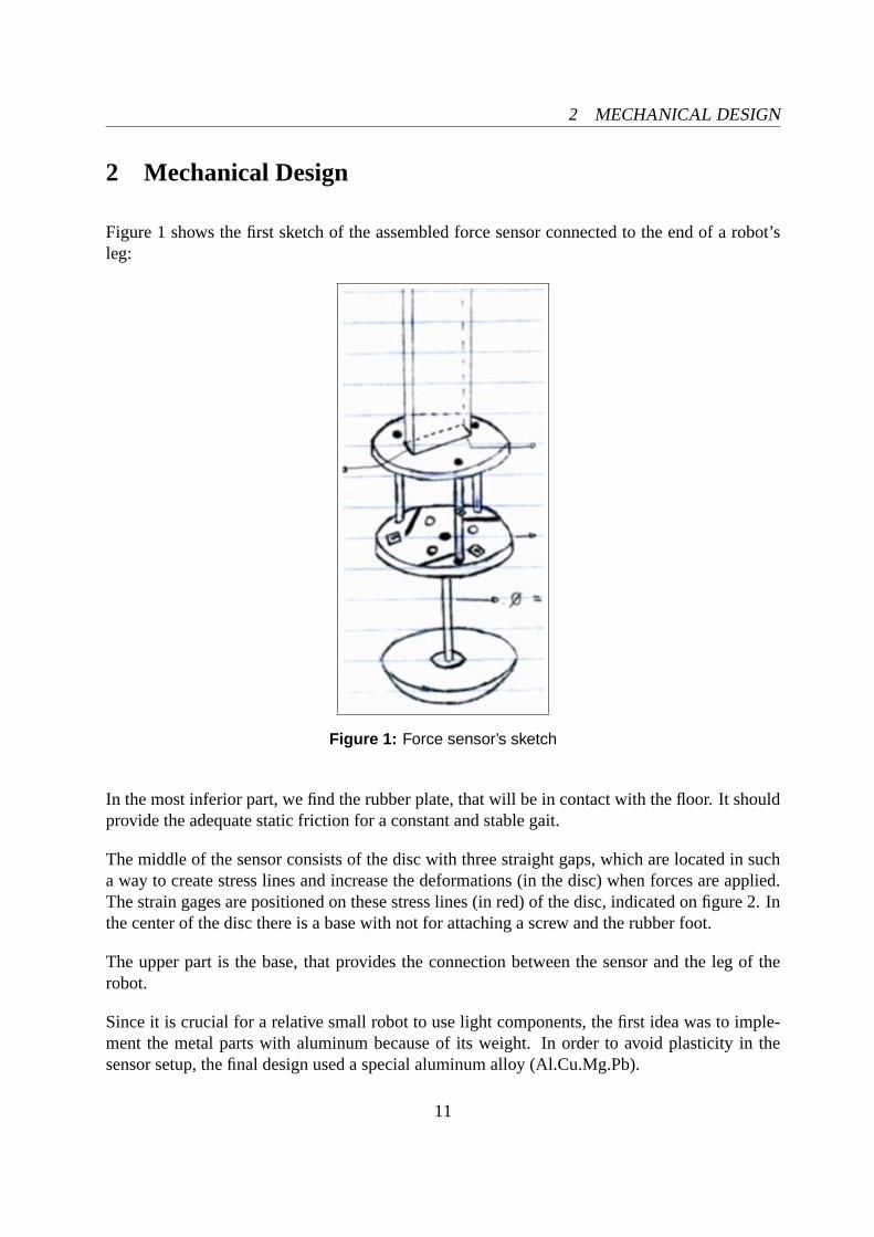
Figure 1 shows the first sketch of the assembled force sensor connected to the end of a robot’sleg:

Figure 1: Force sensor’s sketch

In the most inferior part, we find the rubber plate, that will be in contact with the floor. It shouldprovide the adequate static friction for a constant and stable gait.

The middle of the sensor consists of the disc with three straight gaps, which are located in sucha way to create stress lines and increase the deformations (in the disc) when forces are applied.The strain gages are positioned on these stress lines (in red) of the disc, indicated on figure 2. Inthe center of the disc there is a base with not for attaching a screw and the rubber foot.

The upper part is the base, that provides the connection between the sensor and the leg of therobot.

Since it is crucial for a relative small robot to use light components, the first idea was to imple-ment the metal parts with aluminum because of its weight. In order to avoid plasticity in thesensor setup, the final design used a special aluminum alloy (Al.Cu.Mg.Pb).

11

2 MECHANICAL DESIGN

Below in figure technical the technical drawing that was used to produce the mechanical partsof the sensor can be seen. The dimensions were estimated to measure forces between 0 and1.75[kg]*9,8m

s2 in all directions (maximal forces during the walking). The original FZI designhad to be adapted for a much smaller robot, changing accordingly the diameter and the thicknessof the disc, base and rubber foot.

Figure 2: Technical drawing of the sensor disc and base

12

2.1 Calculation of the 3D forces from the sensor signals 2 MECHANICAL DESIGN

2.1 Calculation of the 3D forces from the sensor signals

Three groups of strain gages set up the vertices of a virtual triangle plain. Forces that act on thedisc change the signals of the strain gages, lifting or lowering the vertices of this triangle. Thecross product theory is been used to calculate the normal vector on this plain, indicating the forcedirections and X, Y and Z components in the sensor’s coordinate system.

2.1.1 Geometry

Picture 3 shows one schematic of the disc with three gaps positioned in the coordinate system ofTarry. Analyzing it´s geometry we can findx, y andz components of each group of strain gages.

The z answers are the derivation of the outputs of the strain gages (-∆V). The minus signal isto adequate the electronics into Tarry´s coordination system. The outputs values of the StrainGages should increase when forces are been applied in Z axis.

X axis

Y axis

Z axis

130 mm

145 mm

75mm

Strain Gage 1Strain Gage 2

Strain Gage 3

Figure 3: The disc with Tarry´s coordinate system

StrainGage1 =

∣∣∣∣∣∣∣

1.30.75−∆V1

∣∣∣∣∣∣∣.

StrainGage2 =

∣∣∣∣∣∣∣

−1.30.75−∆V2

∣∣∣∣∣∣∣.

13


StrainGage3 =

∣∣∣∣∣∣∣

0−1.45−∆V3

∣∣∣∣∣∣∣.

These three 3D points work as vertices of a virtual triangle plain. The normal vector to this plainwill be used to calculate the forces in three axis.

Note that were are mixing different units (Volts and Centimeters). In order to find the rightproportions between them , a calibration will be later necessary (section 4).

2.1.2 Calculation of the virtual plain

In order to create a plain with the strain gages, the three 3D points of Geometry were used tocreate two vectors:

−−−−−−−−−→S.G.2 − S.G.1 =

−−−→S.G12 = x ∗ −2.6 + y ∗ 0 + z ∗ (−∆V2 + ∆V1) (1)

−−−−−−−−−→S.G.3 − S.G.1 =

−−−→S.G13 = x ∗ −1.3 + y ∗ −2.2 + z ∗ (−∆V3 + ∆V1) (2)

2.1.3 Calculating the normal vector on the plain

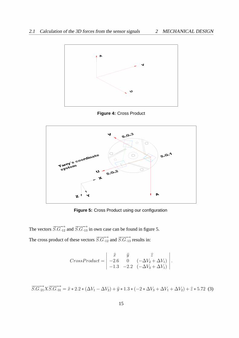
According to section 2.1, the idea here is to find the components of the normal vector on thesame plain as the plain created by the strain gages.

In picture 4, A is the normal vector on the plain defined by U and V. Thex, y andz componentsof A can be calculated using the cross product between U and V. The length of the normal vectoris equal to the area of the parallelogram set up by

−→U and

−→V . This area is meaningless here.

For vectors−→U and

−→V , the cross product is defined below:

−→U X

−→V =

∣∣∣∣∣∣∣

x y zUx Uy Uz

Vx Vy Vz

∣∣∣∣∣∣∣.

−→U X

−→V = x*(Uy*Vz - Uz*Vy) + y*(Uz*Vx - Ux*Vz) + z*(Ux*Vy - Uy*Vx)

14


Figure 4: Cross Product

Figure 5: Cross Product using our configuration

The vectors−−−−→S.G.12 and

−−−−→S.G.13 in own case can be found in figure 5.

The cross product of these vectors−−−−→S.G.12 and

−−−−→S.G.13 results in:

CrossProduct =

∣∣∣∣∣∣∣

x y z−2.6 0 (−∆V2 + ∆V1)−1.3 −2.2 (−∆V3 + ∆V1)

∣∣∣∣∣∣∣.

−−−−→S.G.21X

−−−−→S.G.31 = x ∗ 2.2 ∗ (∆V1 −∆V2) + y ∗ 1.3 ∗ (−2 ∗∆V3 + ∆V1 + ∆V2) + z ∗ 5.72 (3)

15


The number 5.72 inz in equation (3) is meaningless here. Equation (4) is used to calculate theforces in Z direction instead, and after a calibration was done to find the right relation gainsbetweenx, y andz.

Z =WheatstoneBridge1 + WheatstoneBridge2 + WheatstoneBridge3

3(4)

16

3 ELECTRICAL PARTS

3 Electrical Parts

Strain gages were applied forming three full Wheatstone Bridges to transform the mechanicalbending of the metal disc into signals. The voltage signals from the Whetstone Bridges areamplified and filtered with an appropriate circuit. The outputs of this circuit are feed to an ADconverter card, and after used in Tarry´s program in the PC.

The block diagram of this signal processing can be seen in figure 6.

Figure 6: Electrical block diagram

3.1 Strain Gages

Strain gages measure small changes in the resistance of small wires according to their lengthchanges. The strain gages are very often a plastic substrate on with a long wire is put in a meandershape. This substrate is fixed (glued) on the workpiece or device subjected to mechanical stress.When a force is applied to the device, its dimensions will change slightly (assuming we stay inthe linear region of the material).

As the dimensions change (either extension or compression), the dimensions of the strain gageattached to the device also changes. As the length of the wire of the strain gage changes, it’sresistance changes accordingly (again slightly). By measuring this small change in resistance,

17

3.1 Strain Gages 3 ELECTRICAL PARTS

Figure 7: Typical Strain Gages

one can determine the change in the dimension of the device. A Wheatstone Bridge is used tomeasure this small change in resistance.

3.1.1 Chosen Strain Gage Model

The chosen model was a double Strain Gage from HLH, so instead of a total of twelve, a fullWheatstone bridge can then be constructed from six strain gages.

Type: FAE2-A6231J-100-S13E

Basic Gage Factor: 2.05 +/- 0.5%

Maximum Resistance: 1000Ohms +- 0.2%

Gage Length: 3.18mm

Elongation: -0.5%

Figure 8: Chosen Strain Gage

18

3.2 Wheatstone Bridge 3 ELECTRICAL PARTS

3.2 Wheatstone Bridge

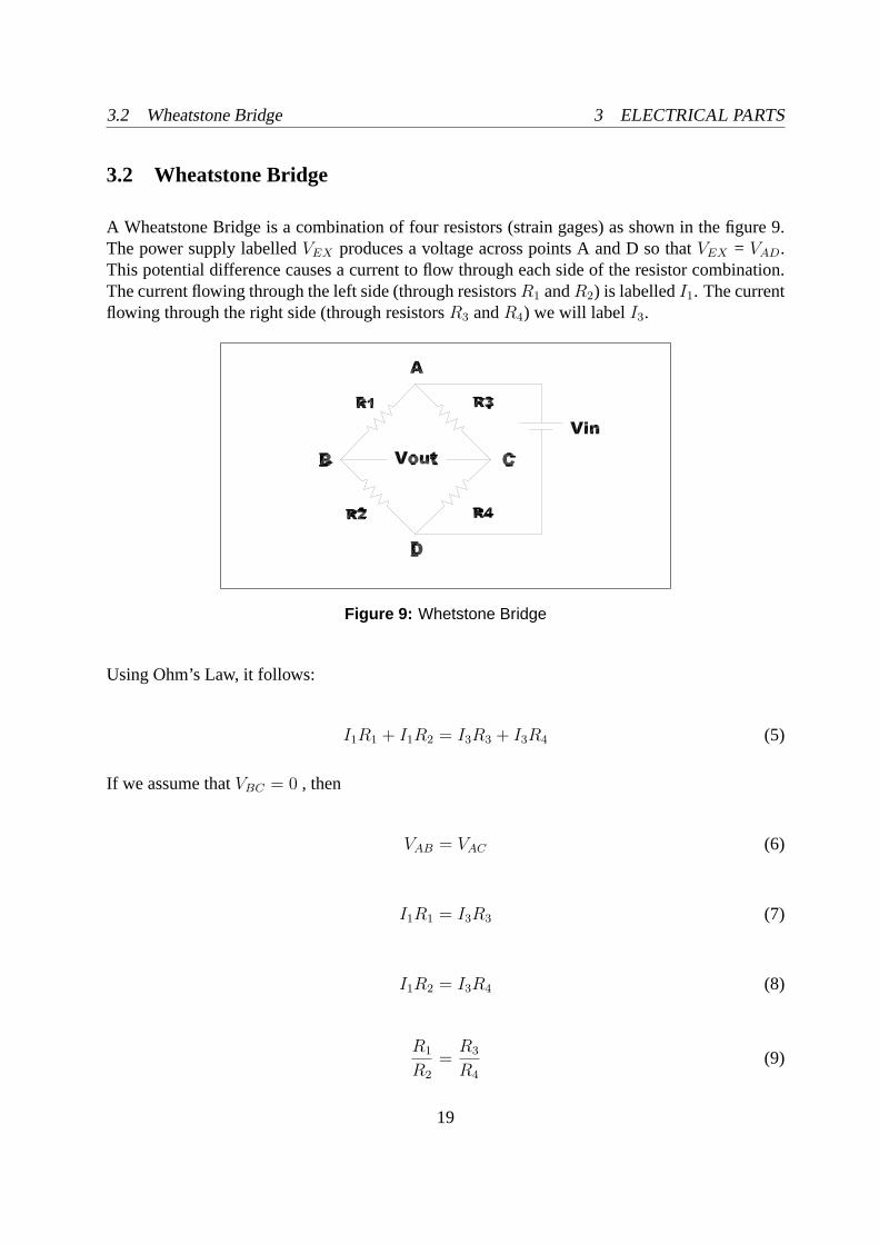
A Wheatstone Bridge is a combination of four resistors (strain gages) as shown in the figure 9.The power supply labelledVEX produces a voltage across points A and D so thatVEX = VAD.This potential difference causes a current to flow through each side of the resistor combination.The current flowing through the left side (through resistorsR1 andR2) is labelledI1. The currentflowing through the right side (through resistorsR3 andR4) we will label I3.

Figure 9: Whetstone Bridge

Using Ohm’s Law, it follows:

I1R1 + I1R2 = I3R3 + I3R4 (5)

If we assume thatVBC = 0 , then

VAB = VAC (6)

I1R1 = I3R3 (7)

I1R2 = I3R4 (8)

R1

R2

=R3

R4

(9)

19


If we divide the equation (6) by equation (7), we get (8).

R3 = R4 ∗ R1

R2

(10)

The output of an unbalanced bridge (Vout ) can be expressed in terms of both the∆RR

and thevoltage input (Vin ), and is commonly taken as proportional to both of them, although the rela-tionship is slightly nonlinear for certain configurations.

In a simplified form (ignoring nonlinearity) the output for a single active strain gage (one arm ofthe bridge is a strain gage subjected to strain, and the other three arms are inactive strain gagesor resistors) can be expressed as:

Vout =Vin

4∗ ∆R

R(11)

or, substituting the Gage Factor equation:

∆R

∆= GF ∗ ∆L

L(12)

then:

Vout =Vin

4∗GF ∗ ∆L

L=

Vin

4GF ∗ ε (13)

Whereε is strain. A second approach, used here, is based on an analysis of voltages and may besomewhat easier for the reader to follow. In the following this approach is shown:

When two resistors,R1 andR2, are placed in series across a constant voltage supply, V.in, asa single voltage divider, they function as a voltage divider with a portion of the supply voltagedropped acrossR1 and the rest acrossR4:

Vin = VR1 + VR4 (14)

Where:

VR1 = Vin ∗ R1

R1 + R4

(15)

20


VR4 = Vin ∗ R4

R1 + R4

(16)

When two more resistors,R2 andR3, are also placed across the same voltage supply, they func-tion as a second parallel voltage divider:

Vin = VR2 + VR3 (17)

Where:

VR2 = Vin ∗ R2

R2 + R3

(18)

VR3 = Vin ∗ R3

R2 + R3

(19)

Depending upon the values of the four resistors, a differential voltage can also be present betweenpoints A and C within this dual voltage divider circuit as a differential voltage output. Thisvoltage,Vout, can be accurately measured with a good high-impedance voltmeter. It can also bedetermined by taking the difference in the voltage drops across the resistors between points Aand C:

Vout = (VR1 − VR2) = (VR3 − VR4) (20)

By substitution of equations (14) and (17), the output can be related to the input voltage and thefour resistances:

Vout = Vin ∗ [R1

R1 + R4

− R2

R2 + R3

] (21)

It should be clear by inspection that the Wheatstone bridge circuit (drawn in the traditional ”di-amond” configuration ) is actually a parallel pair of series voltage dividers like that shown inthe previous figure for differential voltage output. With this identity in mind, it should be alsoobvious thatVout is the voltage output across the signal corners of the Wheatstone bridge andthatVin in is the voltage input across the power corners of the bridge. And the four resistancesrepresent the individual resistances of the four bridge branches.

Equation (21) is the key relationship to understanding the Wheatstone bridge. With it, the outputof the bridge can be found for any combination of input voltage and branch resistances.

21


3.2.1 Configuration - Full Bridge with Dummy Strain Gages

In our sensor, we are using three full bridges implemented like the schematic in figure 10. Look-ing at the equation (21), we can see that the ipsilateral strain gages tend to cancel each other, andthis is a really useful property to compensate the effects of resistance change due to temperaturechanges.

With one strain gage located exactly above the other, the effect of the material deformationcaused by temperature is cancelled out, because it is the same for all the disc, and therefore actson all strain gages. On the other hand, the effects of the deformation caused by external forcesare added, because they are inverse in each side of the disc (for example, the upper part is beingprolonged, and the lower part is being compressed). This kind of configuration is called dummystrain gages.

Figure 10: Dummy Strain Gages

22

3.3 Amplifier Circuit 3 ELECTRICAL PARTS

3.3 Amplifier Circuit

The circuit below provides the offset for the three wheatstone bridges, amplifies and filters thesignals and provides three analog outputs signals, one for each bridge, that go from 0 to 10 Volts.

Figure 11: Amplifier Circuit

The amplifier that is used for the output of each Wheatstone Bridge is the AD623A instrumenta-tion amplifier. Equation (22) gives the gain of this amplifier.

Vout

Vin

= (1 +100K.ohms

RG

) (22)

Currently,RG is 120Ω, which results a gain of 834.334. This is set to reach saturation of theamplifier when 1700 grams are applied to the sensor.

23


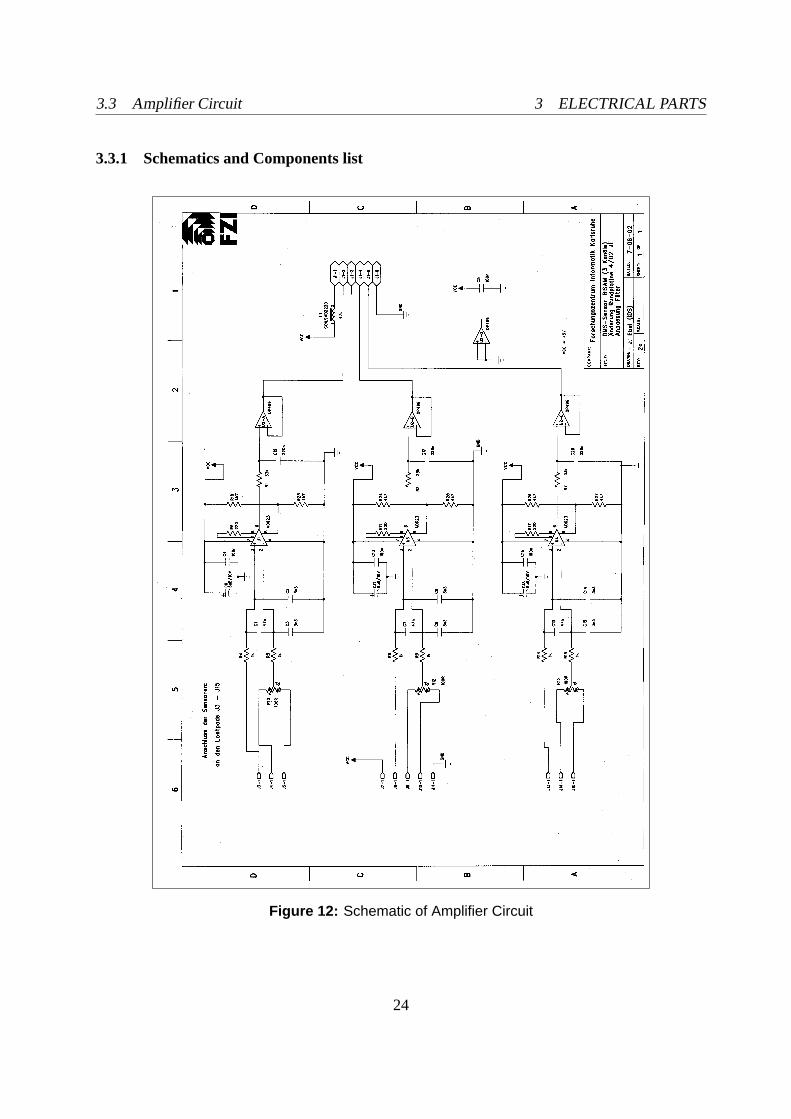
3.3.1 Schematics and Components list

Figure 12: Schematic of Amplifier Circuit

24


Component List:

Figure 13: Components of the circuit

Observation: ComponentsR6, R11 andR17 of figure 13 are changed to120Ω.

25

3.4 Auxiliary Circuit 3 ELECTRICAL PARTS

3.4 Auxiliary Circuit

Figure 14 shows the auxiliary circuit that simplifies the connections between the Wheatstonebridges and the amplifier circuit.

Varnished magnetic wires are soldered between the strain gages and this auxiliary circuit. Thesewires are also glued with silicon in the disc with gaps near the strain gages. This was done inorder to avoid propagation of forces from the wires to the strain gages, changing the answer ofthe sensor.

A cable connects this circuit and the amplifier board. The auxiliary board is attached in the baseof the sensor, using velcro.

Figure 14: Auxiliary Circuit

Figure 15: Schematic of Auxiliary Circuit

26

3.5 A/D Converter Card 3 ELECTRICAL PARTS

Figure 16: Auxiliary Circuit fixed in the base of the sensor with velcro

3.5 A/D Converter Card

The A/D Converter Card transforms the three analogs outputs from the amplifier circuit (0 to 10Volts) into three digital signals, with the rang of 0.00 to 4040.00 . The model of the A/D cardthat is been used in the PCI-1720 Advantech.

Tarry needs to be always connected by cables into a PC, that is responsible for all the processingand control of the robot. With all the necessary conversions during the walking of the robot, theA/D card can measure the three channels of the force sensor in approximately 0.025 seconds,that gives a frequency of 40 Hertz.

27

4 CALIBRATION

4 Calibration

In section (2.1.3) it was explained how to acquire the normal vector from the virtual plain. Thisvector (equation 3) just gives the relationship between the three strain gages groups to calculateanswers in X and Y direction. Another equation (4) is used for Z direction.

The module of these components of the vector have the wrong proportion between each other,resulting in a measured vector with wrong length and direction. The answers do not correspondto any measuring unit.

Therefore calibration was necessary for all directions, determining first one equation intoz foreach group of strain gages, and after special equations for X and Y axis. Just with that plusequations 3 and 4, it is possible to transform the output signals of the strain gages into the correct3D vector in a know unit.

The calibration process works with different weights which are applied to the sensor. The cali-bration results in a curve relating digital values of the measurement to weights in grams. In orderto set a force calibration in Newtons, the results have only to be divided by 1000 ( transforminggrams into kilograms) and multiplied by 9.81m

s2 .

4.1 Implementing the Calibration Function

The calibration function enables the user to put different weights to the senor in X, Y and Z-directions. When the user applies a weight, a button muss be pressed. The corresponding digitalvalues are saved to a file. Later on the user only has to put the value of the applied weightsinto the same file. Using another software like MS Excel or Origin a linear regression can becalculated on these data. The result is a function that takes digital values from the AD-convertercard and returns the resulting force applied.

4.2 Calibration Apparatus

Considering that the strain gages are really sensible, it is crucial to have a precise calibrationapparatus in order to find the exact equations for the forces in the three axis.

Such a precise calibration apparatus was custom built for the force sensor presented here. Itconsists of a metal table with three screws for levelling, one rod with wheel to support a weightat a string and one Dividing Heads to fix, rotate and incline the sensor in relationship to Z axis.

28

4.2 Calibration Apparatus 4 CALIBRATION

Figure 17: Calibration Apparatus

Figure 18: Details: bag with spring, screw for alignment and rod for laying theweight

29


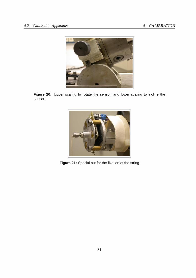
The Dividing Heads has two degrees of freedom, one to rotate the sensor around the Z axis andthe second to incline the orientation of the sensor. Combining these two allows to apply forcesin a half sphere, considering the sensor as being the center of it.

The detailed setup consists of a bag that can contain different known weights. This plastic bagis connected to a string via a spring ( to avoid deformations of the sensor caused by impacts of afalling weight). The string runs over a supporting wheel and ends at the sensor.

The string is connected to the sensor with the help of a special nut that sits on the center of thescrew (where normally the rubber foot is attached). This construction allows the sensor to beexposed to pulling forces. Due to the two degrees of freedom, that were described above, thesepulling forces can point in any direction of a half sphere.

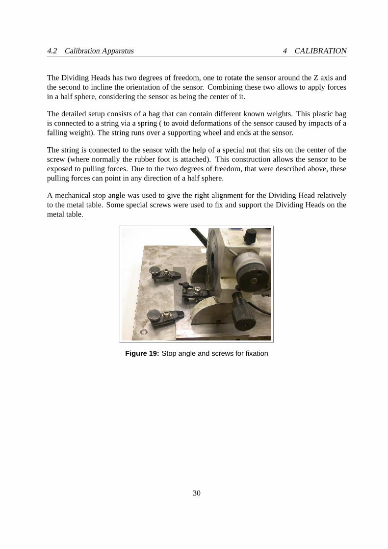
A mechanical stop angle was used to give the right alignment for the Dividing Head relativelyto the metal table. Some special screws were used to fix and support the Dividing Heads on themetal table.

Figure 19: Stop angle and screws for fixation

30


Figure 20: Upper scaling to rotate the sensor, and lower scaling to incline thesensor

Figure 21: Special nut for the fixation of the string

31

4.3 Achieving the desirable angle of inclination to Z direction 4 CALIBRATION

4.3 Achieving the desirable angle of inclination to Z direction

The calibration apparatus was used to apply forces on the sensor in different orientations. Itshould be possible to configure the dispositive in such a way to apply these forces in the exactlyinclination and rotation desired.

890 mm

890 mm

1895 mm

2094 mmL mm

5502 mm

5429 mm

A°

B°

Y°

25.16°

X°

Figure 22: Geometry of the apparatus

Looking to the construction of the hole apparatus (figure 22), we can verify that is not possibleto use directly the scale of the dividing heads to apply the forces with the right inclination on thesensor.

The idea here is to use a equation that gives the length of the string, from the nut of the sensoruntil the red wheel, according to the inclination angle of the force.

The red triangle (figure 22) contains the relationship between the length of the string and thedirection of applied forces. Using these relations we can find the correct length of the stringrequested to exercise the forces in desirable inclinations to Z axis.

In our case, we applied the force using angles of 30 and 60 degrees of inclination (to Z axis).

4.3.1 30 equations

In order to apply forces in 30 of inclination to Z axis in to the sensor (X = 30 in picture 22),the angle used in Y is 124.84, according to the geometric propriety 25.16 + X + Y = 180.

Using the sin relationship:sin(124.84)

55.02=

sin(A)

20.94(23)

32

4.3 Achieving the desirable angle of inclination to Z direction 4 CALIBRATION

A = 18.2

Basic triangle propriety:A + B + 124.84 = 180 (24)

B = 36.96

And sin relationship again:sin(124.84)

55.02=

sin(36.96)

L(25)

L = 40.3 cm

4.3.2 60 equations

To apply forces in 60 of inclination to Z axis in to the sensor(X = 60 in picture 22), the angleused in Y is 94.84, according to the geometric propriety 25.16 + X + Y = 180.

sin(94.84)

55.02=

sin(A)

20.94(26)

A = 22.29

A + B + 94.84 = 180 (27)

B = 62.87

sin(94.84)

55.02=

sin(62.87)

L(28)

L = 49.14 cm

33

4.4 Calibration Procedure 4 CALIBRATION

4.4 Calibration Procedure

As it can be seen in equation (4), the Z-axis of the force depends equally on all three strain gages.In order to calibrate this Z-component the Dividing Heads was brought into a configuration wherethe string pulls directly in the sensor’s Z-direction. This is shown in figure 23. With the help ofthis setup nine different weights were applied to the sensor via string and plastic bag. For eachof these weights the measurements were performed three times, always rotating 120 around theZ-axis between each measurement. This was done in order to cancel out the effects of slightmisalignments of the calibration setup.

Figure 23: Calibration in Z direction

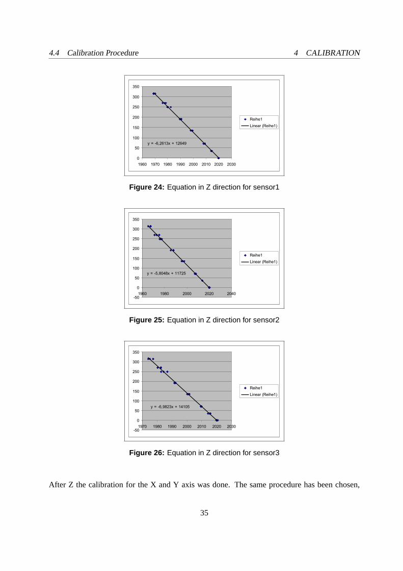
For each full Wheatstone Bridge was calculated one calibration equation (one gain and one offsetfor each sensor) to transform the digital values into grams. The three resulting equations and theunderlying measurements are shown in figures 24, 25 and 26. The Y-axis of each diagram isthe applied weight in grams. The X-axis of each diagram is the corresponding digital valuesthat were measured. As it can be clearly seen in the three figures, each calibration equation is astraight line whose function Y = f(x) is given in the diagrams. The answer in Z direction is themean value of the three Wheatstone Bridges (equation 4).

34


y = -6,2613x + 12649

0

50

100

150

200

250

300

350

1960 1970 1980 1990 2000 2010 2020 2030

Reihe1

Linear (Reihe1)

Figure 24: Equation in Z direction for sensor1

y = -5,8048x + 11725

-50

0

50

100

150

200

250

300

350

1960 1980 2000 2020 2040

Reihe1

Linear (Reihe1)


y = -6,9823x + 14105

-50

0

50

100

150

200

250

300

350

1970 1980 1990 2000 2010 2020 2030

Reihe1

Linear (Reihe1)


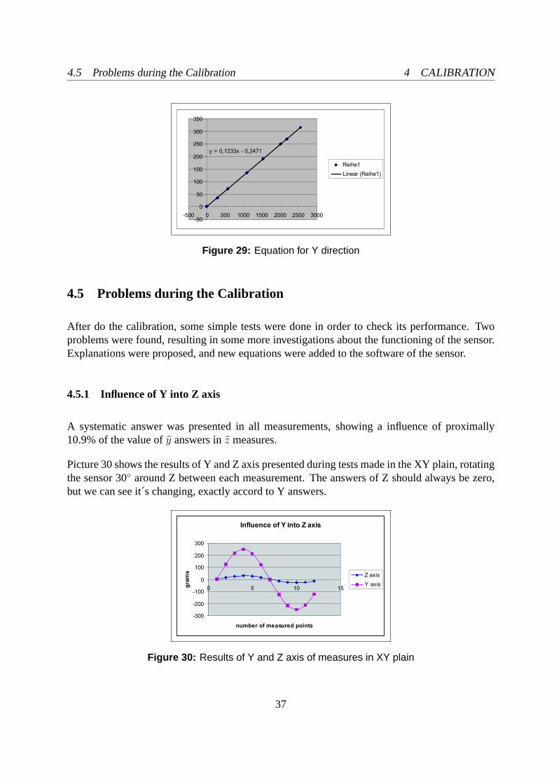
After Z the calibration for the X and Y axis was done. The same procedure has been chosen,

35


but now each weight was measured only once for the X and once for the Y direction. This is asimple calibration because it just consists of finding the appropriate gains for the equation (3),using the already done calibration for the Z axis.

Figure 27: Calibration in XY plain

y = 0,1319x - 0,3288

-50

0

50

100

150

200

250

300

350

-500 0 500 1000 1500 2000 2500 3000

Reihe1

Linear (Reihe1)

Figure 28: Equation for X direction

36

4.5 Problems during the Calibration 4 CALIBRATION

y = 0,1233x - 0,2471

-50

0

50

100

150

200

250

300

350

-500 0 500 1000 1500 2000 2500 3000

Reihe1

Linear (Reihe1)

Figure 29: Equation for Y direction

4.5 Problems during the Calibration

After do the calibration, some simple tests were done in order to check its performance. Twoproblems were found, resulting in some more investigations about the functioning of the sensor.Explanations were proposed, and new equations were added to the software of the sensor.

4.5.1 Influence of Y into Z axis

A systematic answer was presented in all measurements, showing a influence of proximally10.9% of the value ofy answers inz measures.

Picture 30 shows the results of Y and Z axis presented during tests made in the XY plain, rotatingthe sensor 30 around Z between each measurement. The answers of Z should always be zero,but we can see it´s changing, exactly accord to Y answers.

Influence of Y into Z axis

-300

-200

-100

0

100

200

300

0 5 10 15

number of measured points

gra

ms

Z axis

Y axis

Figure 30: Results of Y and Z axis of measures in XY plain

37


To solve that the relation below was added into the calibration software.

X = A;

Y = B;

Z = C - 0.10876*B;

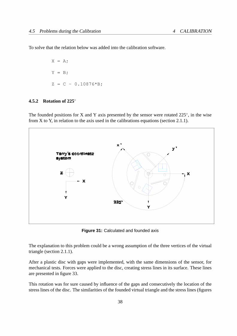
4.5.2 Rotation of 225

The founded positions for X and Y axis presented by the sensor were rotated 225, in the wisefrom X to Y, in relation to the axis used in the calibrations equations (section 2.1.1).

Figure 31: Calculated and founded axis

The explanation to this problem could be a wrong assumption of the three vertices of the virtualtriangle (section 2.1.1).

After a plastic disc with gaps were implemented, with the same dimensions of the sensor, formechanical tests. Forces were applied to the disc, creating stress lines in its surface. These linesare presented in figure 33.

This rotation was for sure caused by influence of the gaps and consecutively the location of thestress lines of the disc. The similarities of the founded virtual triangle and the stress lines (figures

38


32 and 33 are obvious. Unfortunately it is not simple to show mathematically the relationsbetween the stress lines and the position of the strain gages on the disc, creating the virtualtriangle used for the orientation of the sensor (section 2.1). Because of the lack of time, no moretests were done to prove this theory.

Figure 32: First assuming and supposed right orientation of the virtual triangle

Figure 33: Position of stress lines when forces are been applied

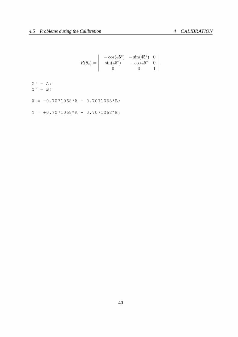
To solve that equations were used in the program for Tarry, adjusting the coordinate system ofthe sensor to Tarry´s. Applying the Rotation Matrix [15], we can obtain the necessary relationsto rotate the axis:

39


R(θz) =

∣∣∣∣∣∣∣

− cos(45) − sin(45) 0sin(45) − cos 45 0

0 0 1

∣∣∣∣∣∣∣.

X‘ = A;Y‘ = B;

X = -0.7071068*A - 0.7071068*B;

Y = +0.7071068*A - 0.7071068*B;

40

5 SOFTWARE

5 Software

In order to calibrate and test the 3D-foot force sensor two software functions have been imple-mented.The first one is a test function which enables the user to collect data during tests when thesensor was exposed to different forces in different directions within a half sphere ( half spherebecause only pulling orientation can be tested with the calibration apparatus). The second one isonly the application of the final calibration formulas within a program that makes Tarry walk ina regular tripod gait. The force sensor was situated at the hind leg of the robot.

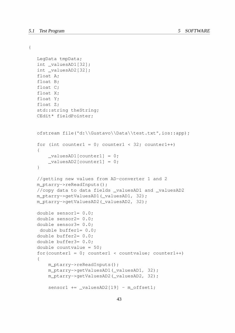
5.1 Test Program

Since it was not clear how good the repetition accuracy of the sensor is, some repetitive tests hadto be performed (see section 6.1).

For these tests a small test function has been been designed. The care of this function is thecalibration function (section 4.1). According to the test pattern described in section 6.1, the userhad to press on offset button between each measurement.This changed the offset of the linearcalibration function. This is exactly the same as somebody does who uses a digital scale andpresses a button to set the tara value.

After that a weight into certain direction is applied to the sensor and the calculated values aresaved to a file.

For this test function a simple graphic interface has been designed. It only consists of an offsetbutton, a button to perform the measurements and save the results, and three displays that showthe correspondent force results in X, Y and Z-direction.

The results which have been achieved can be found in the tests chapter.

void TarryOverviewProp::OnButtonOffset()

LegData tmpData;int _valuesAD1[32];int _valuesAD2[32];

ofstream file("d:\\Gustavo\\Data\\offset.txt",ios::app);

for (int counter1 = 0; counter1 < 32; counter1++)

41

5.1 Test Program 5 SOFTWARE

_valuesAD1[counter1] = 0;_valuesAD2[counter1] = 0;

//getting new values from AD-converter 1 and 2m_ptarry->reReadInputs();//copy data to data fields _valuesAD1 and _valuesAD2m_ptarry->getValuesAD1(_valuesAD1, 32);m_ptarry->getValuesAD2(_valuesAD2, 32);

m_offset1= 0.0;m_offset2= 0.0;m_offset3= 0.0;

double countvalue = 50;for(counter1 = 0; counter1 < countvalue; counter1++)

m_ptarry->reReadInputs();m_ptarry->getValuesAD1(_valuesAD1, 32);m_ptarry->getValuesAD2(_valuesAD2, 32);

m_offset1 += _valuesAD2[19] - 2020;m_offset2 += _valuesAD2[23] - 2020;m_offset3 += _valuesAD2[21] - 2020;

m_offset1 = m_offset1/(1.0*countvalue);m_offset2 = m_offset2/(1.0*countvalue);m_offset3 = m_offset3/(1.0*countvalue);

file << setw(15) << m_offset1<< setw(15) << m_offset2

<< setw(15) << m_offset3<< "\n";

//flush and close the filefile.flush();file.close();

void TarryOverviewProp::OnGustavosButton()

42


LegData tmpData;int _valuesAD1[32];int _valuesAD2[32];float A;float B;float C;float X;float Y;float Z;std::string theString;CEdit* fieldPointer;

ofstream file("d:\\Gustavo\\Data\\test.txt",ios::app);

for (int counter1 = 0; counter1 < 32; counter1++)

_valuesAD1[counter1] = 0;_valuesAD2[counter1] = 0;

//getting new values from AD-converter 1 and 2m_ptarry->reReadInputs();//copy data to data fields _valuesAD1 and _valuesAD2m_ptarry->getValuesAD1(_valuesAD1, 32);m_ptarry->getValuesAD2(_valuesAD2, 32);

double sensor1= 0.0;double sensor2= 0.0;double sensor3= 0.0;

double buffer1= 0.0;double buffer2= 0.0;double buffer3= 0.0;double countvalue = 50;for(counter1 = 0; counter1 < countvalue; counter1++)

m_ptarry->reReadInputs();m_ptarry->getValuesAD1(_valuesAD1, 32);m_ptarry->getValuesAD2(_valuesAD2, 32);

sensor1 += _valuesAD2[19] - m_offset1;

43


sensor2 += _valuesAD2[23] - m_offset2;sensor3 += _valuesAD2[21] - m_offset3;

sensor1 = sensor1/(1.0*countvalue);sensor2 = sensor2/(1.0*countvalue);sensor3 = sensor3/(1.0*countvalue);

buffer1 = -(sensor1*6.2613) + 12649.0;buffer2 = -(sensor2*5.8048) + 11727.0;buffer3 = -(sensor3*6.9823) + 14105.0;

A = 0.1319*(buffer1 - buffer2);B = 0.1233*0.57735*( buffer1 + buffer2 - 2*buffer3);C = (buffer1 + buffer2 + buffer3)/3 - 0.10876*B;

X = -0.7071068*A - 0.7071068*B;Y = + 0.7071068*A - 0.7071068*B;Z = C;

theString = convertFloatToString(X);fieldPointer = (CEdit*) GetDlgItem(IDC_AD_ALPHA_HALL6);fieldPointer->SetWindowText(theString.c_str());

theString = convertFloatToString(Y);fieldPointer = (CEdit*) GetDlgItem(IDC_AD_GAMMA_HALL6);fieldPointer->SetWindowText(theString.c_str());

theString = convertFloatToString(Z);fieldPointer = (CEdit*) GetDlgItem(IDC_AD_TARSUS_HALL6);fieldPointer->SetWindowText(theString.c_str());

file << setw(15) << sensor1<< setw(15) << sensor2<< setw(15) << sensor3<< setw(15) << buffer1<< setw(15) << buffer2<< setw(15) << buffer3<< setw(15) << X<< setw(15) << Y

44

5.2 Tarry Program 5 SOFTWARE

<< setw(15) << Z<< "\n";

//flush and close the filefile.flush();file.close();

5.2 Tarry Program

For the Tarry robot it already exists a program that makes the robot walk in a tripod gait. Thatmeans that there are always 3 legs on the floor during each moment of the walking sequence.The sensor was attached to the left hind legs of the robot (figure 52). The functions for gettingthe force values were implemented into this software.

That enabled us to collect the ground reaction forces during the stance phase (leg on the floor)off the legs. During a swing phase (leg in the air) of the left hind leg the offset of the calibrationfunction was reset to a zero value. And them the measurements during the next stance phasestarted again. The results of this walking experiments are discussed in section 6.3.2.

file://Gustavos variablesdouble m_offset1= 0.0;double m_offset2= 0.0;double m_offset3= 0.0;double gustavosLegArray[18];double sensor1= 0.0;double sensor2= 0.0;double sensor3= 0.0;double buffer1= 0.0;double buffer2= 0.0;double buffer3= 0.0;double A= 0.0;double B= 0.0;double C= 0.0;double X= 0.0;double Y= 0.0;double Z= 0.0;file://Gustavos time measurementstartTime = clock()-clock();

45


stopTime = startTime;while ((Zaehler < Schritte) && !IsKeyPressed(VK_ESCAPE))

for(int i=0; i<(int)(PointsPerSecond*GaitParameter.StepDuration); i++)

Pacer++;

if (Mode == E_REGISTRY) RegGetWaGaitParameter(HKEY_LOCAL_MACHINE,"Software\\Tarry\\WalkingLibParam", &GaitParameter);

GaitParameter.StepWidth[1]=GaitParameter.StepWidth[0];GaitParameter.StepWidth[2]=GaitParameter.StepWidth[0];pGaitGen->SetNewGaitParameters(GaitParameter);

int ret = pGaitGen->GetJointAngles(double(i)*time,q);if (ret != -1)

Beep(50,50);

file://for (int j=0;j<10000;j++)// for (int k=0;k<100;k++)// ;

file://copy servo data to extra arrayfor(int counterGustavo = 0 ;counterGustavo < 18; counterGustavo++)

gustavosLegArray[counterGustavo]=(q.col(0)*RADTODEG).data()[counterGustavo];test << setw(15) << gustavosLegArray[counterGustavo];file://cout << "line:" << counterGustavo << setw(15) << gustavosLegArray[counterGustavo] << endl;file://cout << "betaAngle: " << setw(15) << gustavosLegArray[7] << endl;

cout << endl;AdMessung.Get(AdKanal, AdValue, 21);file://AdValue[0] = 54 AdValue[1] = 58 AdValue[2] = 56file://gustavosLegArray[7]for(counterGustavo = 3 ; counterGustavo < 21; counterGustavo++)

test << setw(15) << AdValue[counterGustavo];

46


if(gustavosLegArray[7] > 100.0 ) m_offset1 = AdValue[0] - 2020;m_offset2 = AdValue[1] - 2020;m_offset3 = AdValue[2] - 2020;

sensor1 = AdValue[0] - m_offset1;sensor2 = AdValue[1] - m_offset2;sensor3 = AdValue[2] - m_offset3;buffer1 = -(sensor1*6.2613) + 12649.0;buffer2 = -(sensor2*5.8048) + 11727.0;buffer3 = -(sensor3*6.9823) + 14105.0;

A = 0.1319*(buffer1 - buffer2);B = 0.1233*0.57735*( buffer1 + buffer2 - 2*buffer3);C = (buffer1 + buffer2 + buffer3)/3 - 0.10876*B;

X = -0.7071068*A - 0.7071068*B;Y = + 0.7071068*A - 0.7071068*B;Z = C;

test << setw(15) << sensor1<< setw(15) << sensor2<< setw(15) << sensor3<< setw(15) << X<< setw(15) << Y<< setw(15) << Z<< setw(15) << m_offset1<< setw(15) << m_offset2<< setw(15) << m_offset3;

47

6 TESTS

6 Tests

6.1 Tests for checking the accuracy of the sensor

In order to check the properties of the sensor, considering the length and the directions of theresultant force vector, two weights (135 and 248.4 grams) were measured in 48 different orien-tations using the calibration apparatus. Each of the 48 orientations, for the two weights, wassampled 10 times, which result in a total of 960 samples. The software described in section 5.2was used here.

The first 12 samples were oriented perpendicular to the Z axis. Like it is shown in figure 34,taking as the first sample oriented exactly in X direction, and rotating the apparatus in 30 stepsbetween each measurers around the Z axis in order to get the other 11 samples in this configura-tion.

90°

Figure 34: First 12 points, applying forces perpendicular to Z direction

The 13th. to 24th. point were located in 60 of inclination to Z direction, with a difference of30 between each other (rotation around Z axis). As the first configuration, the 13th. point waslocated in X direction.

48

6.1 Tests for checking the accuracy of the sensor 6 TESTS

60°

Figure 35: Points 13 to 24, applying forces with 60 of inclination to Z direction

The 25th. to 36th. point were located in 30 of inclination to Z direction, with a difference of30 between each other ( rotation around Z axis).

30°

Figure 36: Points 25 to 36, applying forces with 30 of inclination to Z direction

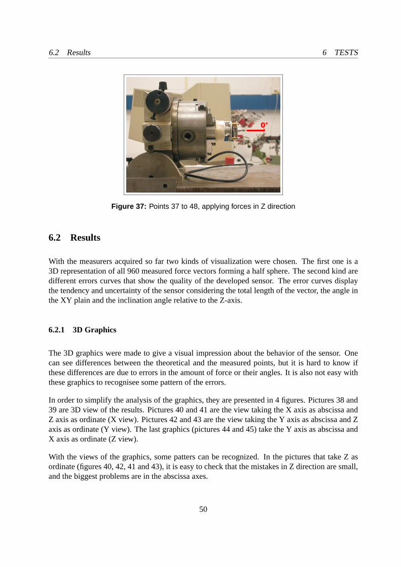
The last 12 points (37th. to 48th.) were located in Z direction, with a difference of 30 betweeneach other ( rotation around Z axis). This rotation has no meaning here, but it has been done justto keep the same pattern.

49

6.2 Results 6 TESTS

0°

Figure 37: Points 37 to 48, applying forces in Z direction

6.2 Results

With the measurers acquired so far two kinds of visualization were chosen. The first one is a3D representation of all 960 measured force vectors forming a half sphere. The second kind aredifferent errors curves that show the quality of the developed sensor. The error curves displaythe tendency and uncertainty of the sensor considering the total length of the vector, the angle inthe XY plain and the inclination angle relative to the Z-axis.

6.2.1 3D Graphics

The 3D graphics were made to give a visual impression about the behavior of the sensor. Onecan see differences between the theoretical and the measured points, but it is hard to know ifthese differences are due to errors in the amount of force or their angles. It is also not easy withthese graphics to recognisee some pattern of the errors.

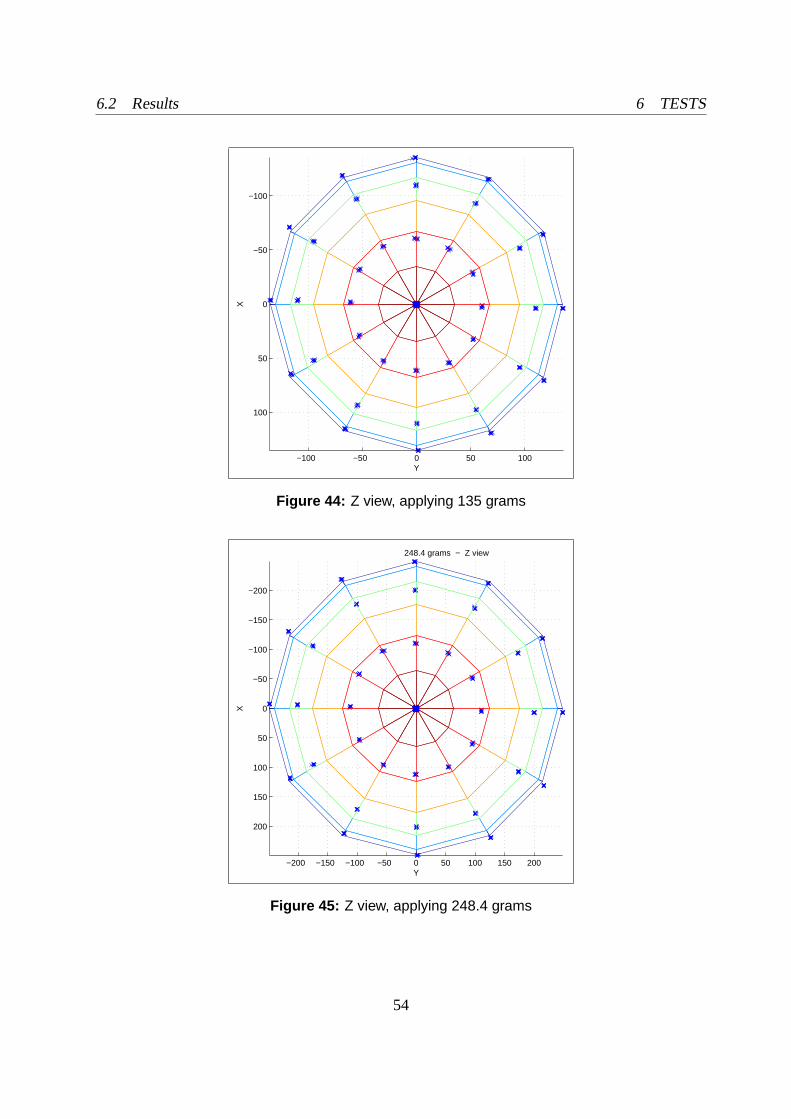
In order to simplify the analysis of the graphics, they are presented in 4 figures. Pictures 38 and39 are 3D view of the results. Pictures 40 and 41 are the view taking the X axis as abscissa andZ axis as ordinate (X view). Pictures 42 and 43 are the view taking the Y axis as abscissa and Zaxis as ordinate (Y view). The last graphics (pictures 44 and 45) take the Y axis as abscissa andX axis as ordinate (Z view).

With the views of the graphics, some patters can be recognized. In the pictures that take Z asordinate (figures 40, 42, 41 and 43), it is easy to check that the mistakes in Z direction are small,and the biggest problems are in the abscissa axes.

50

6.2 Results 6 TESTS

−100

−50

0

50

100

−100

−50

0

50

100

0

20

40

60

80

100

120

XY

Z

Figure 38: 3D view, applying 135 grams

−200−100

0100

200−200−100

0100

200

0

50

100

150

200

250

XY

Z

248.4 grams − Z view

Figure 39: 3D view, applying 248.4 grams

51

6.2 Results 6 TESTS

−100 −50 0 50 100 −1000100

0

20

40

60

80

100

120

YX

Z

Figure 40: X view, applying 135 grams

−200−150−100−50050100150200

0

50

100

150

200

250

YX

Z


Figure 41: X view, applying 248.4 grams

52

6.2 Results 6 TESTS

−100 −50 0 50 1000

20

40

60

80

100

120

Y

Z

Figure 42: Y view, applying 135 grams

−200 −150 −100 −50 0 50 100 150 2000

50

100

150

200

250

Y

Z


Figure 43: Y view, applying 248.4 grams

53

6.2 Results 6 TESTS

−100

−50

0

50

100

−100 −50 0 50 100Y

X

Figure 44: Z view, applying 135 grams

−200

−150

−100

−50

0

50

100

150

200

−200 −150 −100 −50 0 50 100 150 200Y

X


Figure 45: Z view, applying 248.4 grams

54

6.2 Results 6 TESTS

The problem becomes more clear in figures 44 and 45. Here is evident that the measures madein 30 and 60 of inclination to Z have always a small module in X and Y axes, being alwaysinside the theoretical circle.

This problem is was caused by the calibration procedure, and will be more explained in the nextsection.

55

6.2 Results 6 TESTS

6.2.2 Error Curves

The error curves are standard graphics to evaluate the accuracy of any measuring device. Here,one error curve consists of three lines. The middle line is the tendency of the device. That isthe difference between the mean values of the measurements and the real values. The upper andlower lines are the mean value plus and minus the tendency, respectively.

The tendency is the standard deviation multiplied by the Student coefficient (T Student, for tenmeasurements for each point, using a probability of 95%). This means that there is a probabilityof 95% that all the possible results of the measurements will be between these two extreme lines.

In the X axis, we can see the samples, going from 1 to 48 (see section 6.1).

Graphics 46 and 47 show the difference between the real and the measured length of the vector.Length =

√x2 + y2 + z2

Error Curve - Length - (135g)

-12

-10

-8

-6

-4

-2

0

2

4

6

8

1 5 9

13

17

21

25

29

33

37

41

45

Points [1..48]

[gra

ms]

Tendency +

Uncertainty

Tendency

Tendency -

Uncertainty

Figure 46: Error curve of the length of the vector, applying 135 grams

Error Curve - Length - (248,4g)

-20

-15

-10

-5

0

5

10

1 5 9

13

17

21

25

29

33

37

41

45

Points [1..48]

[gra

ms]

Tendency +

Uncertainty

Tendency

Tendency -

Uncertainty

Figure 47: Error curve of the length of the vector, applying 248.4 grams

56

6.2 Results 6 TESTS

We can see again that the biggest mistakes occurred with those points inclined of 30 and 60 tothe Z axis.

This happened because of the influences of the wheel that supports the string which holds thebag with the weight. According to the calibration procedure (section 4.3), just the Z axis wascalibrated laying the weight on the wheel, and X and Y axis were calibrated without it.

During the tests in 30 and 60 of inclination to Z, the weights were supported on the wheel.We can see that the equations used for X and Y axes are not well adequate, because they werecalculated for tests that didn’t use the wheel for supporting the weight.

Laying the weight on the wheel decreases the measured components X and Y of the applied force(using the calibrations described). This affects the total length of the vector. We can even checkthat the mistakes increase in 60 of inclination, when the biggest components of the vector are inXY plain.

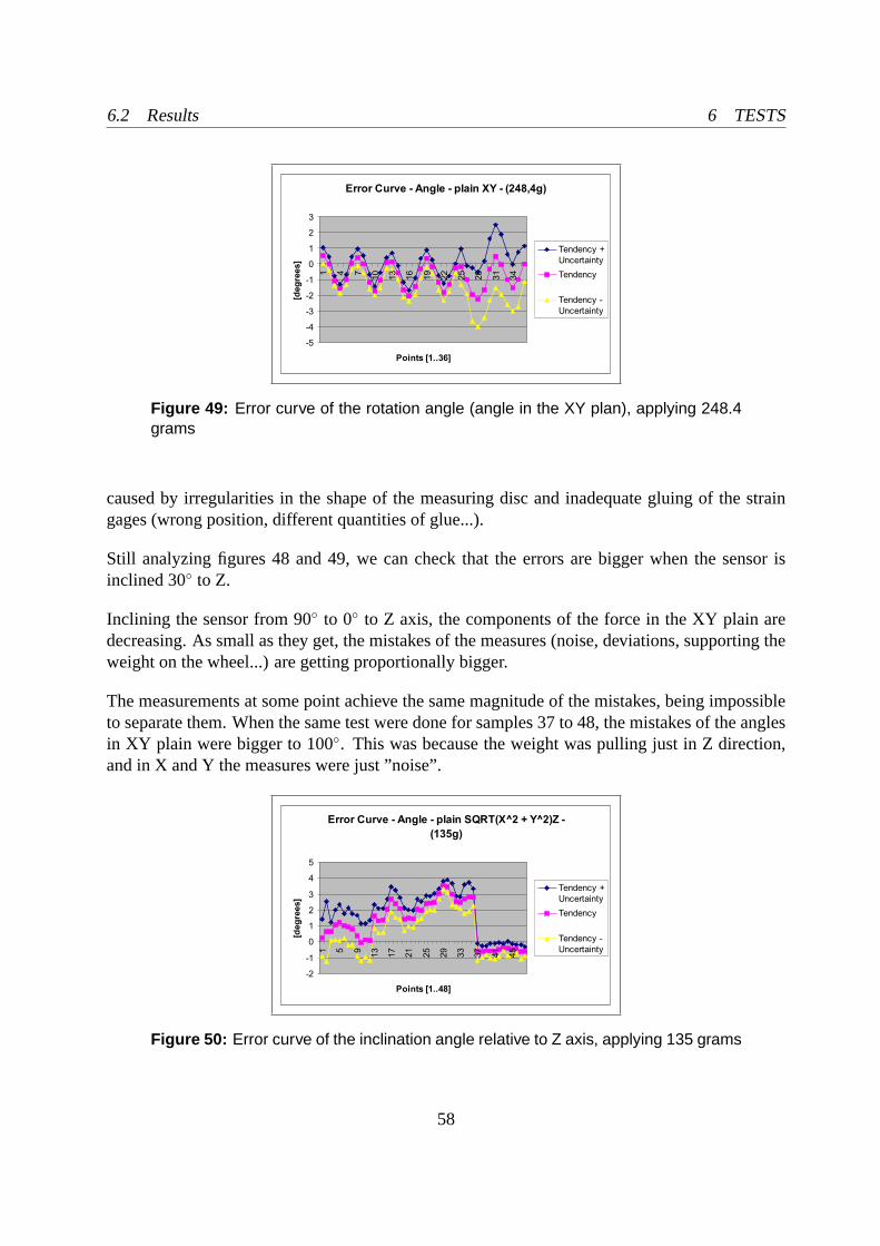
Graphics 48 and 49 are related to the angle of the vector in the XY plain. Angle in XY plain =tanh(Y/X)

Error Curve - Angle - plain XY - (135g)

-5

-4

-3

-2

-1

0

1

2

3

4

1 4 7

10

13

16

19

22

25

28

31

34

Points [1..36]

[deg

rees]

Tendency +

Uncertainty

Tendency

Tendency -

Uncertainty

Figure 48: Error curve of the rotation angle (angle in the XY plan), applying 135grams

One important difference in these graphics is that the samples in X axis are from 1 to 36. Thesamples 37 to 48 are located in Z direction, and there is no mean to check the angles in the XYplain for one vector that is pure orientated into Z (orthogonal between them).

It is easy to check the periodic behavior of these graphics. Two points of maximum and minimumare detected for each complete turn of the sensor.

Further test present an angle of 89 between X and Y axes. This represents a misalignment of 1

in the orthogonality between X and Y axis.

These problems can be explained by some asymmetry of the sensor. These asymmetries are

57

6.2 Results 6 TESTS

Error Curve - Angle - plain XY - (248,4g)

-5

-4

-3

-2

-1

0

1

2

3

1 4 7

10

13

16

19

22

25

28

31

34

Points [1..36]

[deg

rees]

Tendency +

Uncertainty

Tendency

Tendency -

Uncertainty

Figure 49: Error curve of the rotation angle (angle in the XY plan), applying 248.4grams

caused by irregularities in the shape of the measuring disc and inadequate gluing of the straingages (wrong position, different quantities of glue...).

Still analyzing figures 48 and 49, we can check that the errors are bigger when the sensor isinclined 30 to Z.

Inclining the sensor from 90 to 0 to Z axis, the components of the force in the XY plain aredecreasing. As small as they get, the mistakes of the measures (noise, deviations, supporting theweight on the wheel...) are getting proportionally bigger.

The measurements at some point achieve the same magnitude of the mistakes, being impossibleto separate them. When the same test were done for samples 37 to 48, the mistakes of the anglesin XY plain were bigger to 100. This was because the weight was pulling just in Z direction,and in X and Y the measures were just ”noise”.

Error Curve - Angle - plain SQRT(X^2 + Y^2)Z -

(135g)

-2

-1

0

1

2

3

4

5

1 5 9

13

17

21

25

29

33

37

41

45

Points [1..48]

[deg

rees]

Tendency +

Uncertainty

Tendency

Tendency -

Uncertainty

Figure 50: Error curve of the inclination angle relative to Z axis, applying 135 grams

58

6.2 Results 6 TESTS

Error Curve - Angle - plain SQRT(X^2 + Y^2)Z -

(248,4g)

-2

-1

0

1

2

3

4

1 5 9

13

17

21

25

29

33

37

41

45

Points [1..48]

[deg

rees]

Tendency +

Uncertanty

Tendency

Tendency -

Uncertainty

Figure 51: Error curve of the inclination angle relative to Z axis, applying 135 grams

Graphics 50 and 51 are related to the angle, in the plain created by√

X2 + Y 2 and Z, of themeasured vector. Angle inZ

√X2 + Y 2 plain =tanh(Z/

√X2 + Y 2)

59

6.3 Tests with TarryIIb 6 TESTS

6.3 Tests with TarryIIb

The tests with Tarry were made using the already existing software for walking and modify it asit is shown in section 5.3. The sensor and the amplifier circuit were attached in the robot at theleft hind leg. Other crucial modification that has to be done was to change the special nut forapplying the pulling forces for a rubber foot.

Figure 52: TarryIIb walking with the 3D foot force sensor

6.3.1 Models of rubber foot

The rubber foot avoids impacts that are destructive for the sensor when hitting the ground. Fur-thermore this foot guarantees the adequate static friction between the foot and the ground sub-strate.

Some models of rubber foot have been tested before the final design was chosen. The parametersanalyzed were stability and adhesion during the walking and uniform propagation of the reactionforce in all directions.

The final model (picture 54) consists in a plastic base with not for screw inside a half sphere ofspecial silicon.

60


Figure 53: First models of the rubber foot

Figure 54: Final design of rubber foot

6.3.2 Results

The results of the measurements done during the walking are presented below. The graphicsshows 18 steps of Tarry. The ordinate axis show the time (in milliseconds). The abscissa showthe result (in grams) of how much force (divided by 9.81m

s2 and multiplied by 1000) is beingapplied inx, y andz, respectively.

According to the coordinate system of Tarry (figure 55), the measurements made during thewalking of the robot presented the expected results.

The graphics show 18 steps of Tarry. When the components of the force are zero, the leg is inthe air, not touching the floor.

In each step, the components of the force in X direction start with a maximum positive signal(leg positioned ahead). During the step they go decreasing until a maximum negative signal(leg positioned ago), with the biggest amplitude value (for being the hind leg, the leg is usually

61


Y

XZ

Figure 55: TarryII and its coordination system

0 200 400 600 800 1000 1200 1400 1600 1800−600

−500

−400

−300

−200

−100

0

100

200

300

Figure 56: Forces in x during steps

inclined back, pushing the robot), when the leg leaves the floor.

Because the sensor is positioned in the left side of the robot, the measurements in Y directionhave almost always positive signals. In the end of a step the measurements show small positiveanswers. We can check this behavior in figure 52, looking to the middle leg. In this point the legin inclined to the robot, presenting positive force in Y direction.

According to the coordinate system, it was expected that all the measurements in Z direction

62


0 200 400 600 800 1000 1200 1400 1600 1800−400

−200

0

200

400

600

800

1000

1200

1400

Figure 57: Forces in y during steps

0 200 400 600 800 1000 1200 1400 1600 1800−1600

−1400

−1200

−1000

−800

−600

−400

−200

0

200

Figure 58: Forces in z during steps

63


have negative signals.

We can check that all the components of the force shows intermediary maximum and minimumintermediary points for each step. This shows the influence of the other legs in the measurements,when they are leaving or touching the floor.

64


6.3.3 Checking the deviation of the calibration equations

During the walking of the robot, the sensor is exposed to lots of impacts caused by the contactbetween the leg and the ground.

One final test was made to verify the deviation of the calibration equations used due to theimpacts. Two new calibrations were made for the sensor, before and after 100 steps of Tarry.

The equations are shown below:

Calibration before 100 steps:

buffer1 = -(sensor1*6.7621) + 13661.0;

buffer2= -(sensor2*6.2731) + 12671.0;

buffer3 = -(sensor3*7.4019) + 14953.0;

A = 0.134*(buffer1 - buffer2);

B = 0.1272*0.57735*( buffer1 + buffer2 - 2*buffer3);

C = (buffer1 + buffer2 + buffer3)/3

-0.1272*0.08264*0.57735*(buffer1 + buffer2 - 2*buffer3);

Calibration after 100 steps:

buffer1 = -(sensor1*6.8782) + 13894.0;

buffer2= -(sensor2*6.3168) + 12759.0;

buffer3 = -(sensor3*7.4428) + 15034.0;

A = 0.1324*(buffer1 - buffer2);

65


B = 0.1262*0.57735*(buffer1 + buffer2 - 2*buffer3);

C = (buffer1 + buffer2 + buffer3)/3

-0.1262*0.08512*0.57735*(buffer1 + buffer2 - 2*buffer3);

This data shows a relative deviation of 13.4% in X axis, 5.16% in Y axis and 1% in Z axis,ignoring the change of offset.

In order to avoid this problem, it is suggested (see section 8.1) to increase the thickness of discwith gaps for the next version of the sensor.

66

7 FINAL PRODUCT

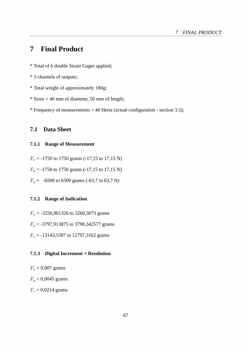
7 Final Product

* Total of 6 double Strain Gages applied;

* 3 channels of outputs;

* Total weight of approximately 180g;

* Sizes = 40 mm of diameter, 50 mm of length;

* Frequency of measurements = 40 Hertz (actual configuration - section 3.5);

7.1 Data Sheet

7.1.1 Range of Measurement

Fx = -1750 to 1750 grams (-17,15 to 17,15 N)

Fy = -1750 to 1750 grams (-17,15 to 17,15 N)

Fy = -6500 to 6500 grams (-63,7 to 63,7 N)

7.1.2 Range of Indication

Fx = -3256,961326 to 3260,3073 grams

Fy = -3797,913875 to 3790,342577 grams

Fz = -13143,5587 to 12797,3162 grams

7.1.3 Digital Increment = Resolution

Fx = 0,007 grams

Fy = 0,0045 grams

Fz = 0,0214 grams

67

7.2 Comparison with other Sensors 7 FINAL PRODUCT

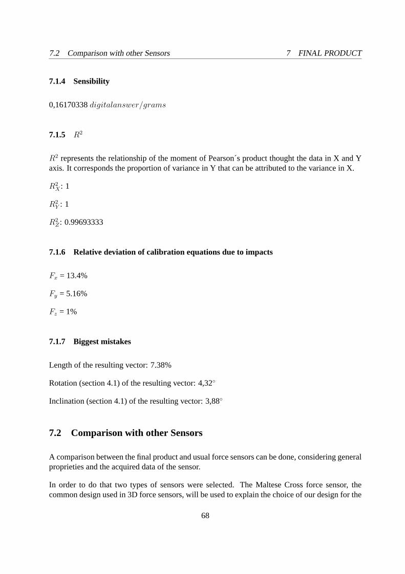
7.1.4 Sensibility

0,16170338digitalanswer/grams

7.1.5 R2

R2 represents the relationship of the moment of Pearson´s product thought the data in X and Yaxis. It corresponds the proportion of variance in Y that can be attributed to the variance in X.

R2X : 1

R2Y : 1

R2Z : 0.99693333

7.1.6 Relative deviation of calibration equations due to impacts

Fx = 13.4%

Fy = 5.16%

Fz = 1%

7.1.7 Biggest mistakes

Length of the resulting vector: 7.38%

Rotation (section 4.1) of the resulting vector: 4,32

Inclination (section 4.1) of the resulting vector: 3,88

7.2 Comparison with other Sensors

A comparison between the final product and usual force sensors can be done, considering generalproprieties and the acquired data of the sensor.

In order to do that two types of sensors were selected. The Maltese Cross force sensor, thecommon design used in 3D force sensors, will be used to explain the choice of our design for the

68


sensor.

A specific model sensor, the most similar possible to find in the ”market”, will work as a referenceof accuracy.

7.2.1 Maltese Cross Force Sensor

In the Maltese Cross force sensor design, the spokes of a wheel are instrumented with gages andcalibrated to measure forces applied to the hub relative to the rim.

Figure 59: Maltese Cross design

In order to measure the force in three axis, four gages are applied to each beam giving a total of8 differential measurements.

This is the reason to decide not to use this common design. The Maltese Cross works with 8basic points, against 3 of the sensor described in this report.

The eight outputs channels of the Maltese sensor are the entry of a matrix that relates the strainmeasurements to forces. Comparing to our sensor, there are 5 more channels been used. Usingforce sensors in all the legs of the robot, this difference results in a economy of 30 channels (48against 18).

Other important economy is related with the Strain Gages, the most expensive part of the ForceSensor. In order to implement one Maltese Cross Force Sensor with the same configurationdescribed here ( full Wheatstone Bridges (section 3.2.1)), 16 double strain gages should be used,versus 6 applied here.

69


The disc with three straight gaps design was chosen for Tarry because of its simplicity. It is easyto realize that three points of reference is the simple possible configuration to determine forcesin three axis.

7.2.2 1D/3D Measuring Wedges - Prometec

After lot´s of research through catalogs of sensors and devices, electronics shops in the IN-TERNET, just one model relatively similar was founded. Normally the sensor´s companies justproduce Force Measuring Devices for one direction, and projected for other landing of weights(kilo Newtons). It seams that small and lightweight 3D force sensors are not expressive items inthe sensor market, and we probably would not find a adequate sensor to by for Tarry.

The selected sensor is called 1D/3D Measuring Wedges, and it is produced by Prometec. TheData Sheet can be found in reference (11).

Even being a small and light 3D force sensor, it is projected to measure forces in the range of 15kN in z, against the 35 N of our sensor. Because of that and few information in the Data Sheet,the comparison between these sensors can not go ahead.

70

8 CONCLUSIONS AND PERSPECTIVES

8 Conclusions and Perspectives

The result of this research was a 3D Foot Force Sensor adequate for the Robot TarryIIb. Thesensor attended to all necessary requisites (simplicity, small size and lightweight, robust andcheap) and presented acceptable accuracy for its application.

During the development of the complete dispositive, several theories and tools from differentareas were used. Knowledge of Mechanics, Geometry and Algebra, Circuits, Electronic, Pro-gramming and Metrology were applied to solve the task. This aspect of the project was reallygrateful, promoting a linking between different subjects boarded during the Engineering Course.

The implementation provided new experiences, integrating theory and practice and giving gen-eral vision about engineering processes.

According to observations made during the implementation, some advices are suggested for thenext version of the force sensor, looking thought increasing its accuracy.

8.1 Improvements for the next version

Two significative problems were identified during the implementation of the sensor. Both prob-lems are caused by the deformation of the disc, changing the efficacious of the calibration equa-tions.

The impact caused by the touch of the sensor with the floor causes great deformation in themeasuring disc. Maximum mistakes of 13% are presented in the module of the components ofthe resulting vector (section 6.3.3). The solution for this problem is to increase the thickness ofthe disc, from 1.5 mm to 2.0 mm.

Forces in the varnished magnetic wires (section 3.4) cause deformation in the measuring disc.Touching the wires can cause maximum mistakes of 10% of the length of the resulting vector.In order to solve this problem a intermediary disc is proposed, guaranteing always the sameconfiguration of the wires between the measuring and this new intermediary disc. Changing thefixation of the auxiliary circuit into the base disc from velcro 16 to screws can also help.

Test were done with a plastic paper measuring disc with the right format, showing lines of moststress. This suggests a better place to glue the Strain Gages in relation to the measuring disc.

These suggestions are shown in figure 60.

Finally, it is possible to have one much more precise dispositive using the same design, correctingthe mistakes explained in section 6.2.2. This could be done by changing the implementation ofthe sensor and the calibration apparatus.

71

8.1 Improvements for the next version 8 CONCLUSIONS AND PERSPECTIVES

Figure 60: Intermediary disc and new version of measuring disc

The dimensions of the discs should be more accurate, and the the gluing of the Strain Gages intothe disc should not be done by hand. The calibration should always be executed in the sameconditions, never laying the weights on a rote with wheel.

Theses improvements are not simple neither cheap to execute, and they are not necessary for theapplication in question.

72

9 REFERENCES

9 References

[1] http://www.uni-bielefeld.de/biologie/Kybernetik/

[2] Cruse, Bartling and Kindermann; High-passfiltered positive feedback; 1995.

[3] Klein and Kittivatcharapong. Forcedistribution problem.

[4] Prof. Augusto Humberto Bruciapaglia. DAS 5101 - Process inEngineering Study Aid.

[5] http://mathworld.wolfram.com/CrossProduct.html

[6]Alfredo Steinbruch and Paulo Winter. Algebra Linear.Makron Books.

[7] http://www.blh.de/

[8] http://ceaspub.eas.asu.edu/imtl/HTML/Manuals/DemoCart_intro.html

[9] http://www.vishay.com/brands/measurements_group/guide/ta/sgms/sgi5.htm

[10] http://www.vishay.com/brands/measurements_group/guide/ta/sgms/wbp2.htm

[11] http://www.analog.com/UploadedFiles/Data_Sheets/516895375AD623_c.pdf

[12] Prof. Armando Albertazzi Goncalves Junior. Metrology StudyAid. Labmetro

[13] http://www.lirmm.fr/manifs/UEE/docs/slides/Hannaford3.pdf

[14] http://www.prometec.com/download/dgb/1D_3D_Meas_Wedges_GB.pdf

[15]L. Sciavicco and B. Siciliano. MOdeling and Control of RobotManipulators. McGraw-Hill Company, Inc., New York, USA, 1996.

73

Date post:	14-Feb-2019
Category:	Documents
Upload:	phungkhanh
View:	213 times
Download:	0 times

Development Software and Control - coep.ufrj.brgfreitas/documentos/relatorio.pdf · ... como por...

Documents