50
DIFFERENTIATION RULES We know that, if y = f (x), then the derivative dy/dx can be interpreted as the rate of change of y with respect to x.
| Date post: | 13-Dec-2015 |
| Category: |
Documents |
| Upload: | brian-hopkins |
| View: | 219 times |
| Download: | 1 times |

DIFFERENTIATION RULES
We know that, if y = f (x), then the derivative
dy/dx can be interpreted as the rate of change of
y with respect to x.

3.7Rates of Change in the
Natural and Social Sciences
In this section, we will examine:
Some applications of the rate of change to physics,
chemistry, biology, economics, and other sciences.
DIFFERENTIATION RULES

Let us recall from Section 2.7 the basic idea
behind rates of change.
If x changes from x1 to x2, then the change in x is ∆x = x2 – x1
The corresponding change in y is ∆y = f(x2) – f(x1)
RATES OF CHANGE

The difference quotient
is the average rate of change of y with respect to x
over the interval [x1, x2]. It can be interpreted as
the slope of the secant line PQ.
2 1
2 1
( ) ( )
f x f xy
x x x
AVERAGE RATE

Its limit as ∆x → 0 is the derivative f '(x1). This can therefore be interpreted as the instantaneous rate of
change of y with respect to x or the slope of the tangent line at P(x1,f (x1)).
INSTANTANEOUS RATE

Using Leibniz notation, we write the process in the
form
0lim
x
dy y
dx x
RATES OF CHANGE

Whenever the function y = f (x) has a specific
interpretation in one of the sciences, its derivative
will have a specific interpretation as a rate of
change.
As we discussed in Section 2.7, the units for dy/dx are the units for y divided by the units for x.
RATES OF CHANGE

We now look at some of these interpretations in
the natural and social sciences.
NATURAL AND SOCIAL SCIENCES
Let s = f (t) be the position function of a particle
moving in a straight line.
Then, ∆s/∆t represents the average velocity over a time period ∆t v = ds/dt represents the instantaneous velocity
(velocity is the rate of change of displacement with respect to time)
The instantaneous rate of change of velocity with respect to time is acceleration: a(t) = v’(t) = s’’(t)
PHYSICS

These were discussed in Sections 2.7 and 2.8 However, now that we know the differentiation formulas,
we are able to solve problems involving the motion of objects more easily.
PHYSICS

The position of a particle is given by the equation
s = f(t) = t3 – 6t2 + 9t
where t is measured in seconds and s in meters.
a) Find the velocity at time t.
b) What is the velocity after 2 s? After 4 s?
c) When is the particle at rest?
PHYSICS Example 1

d) When is the particle moving forward (that is, in the positive direction)?
e) Draw a diagram to represent the motion of the particle.
f) Find the total distance traveled by the particle during the first five seconds.
PHYSICS Example 1

g) Find the acceleration at time t and after 4 s.
h) Graph the position, velocity, and acceleration functions for 0 ≤ t ≤ 5.
i) When is the particle speeding up? When is it slowing down?
PHYSICS Example 1

The velocity function is the derivative of the
position function.
s = f(t) = t3 – 6t2 + 9t
v(t) = ds/dt = 3t2 – 12t + 9
PHYSICS Example 1 a
The velocity after 2 s means the instantaneous
velocity when t = 2, that is,
The velocity after 4 s is:
2
2
(2) 3(2) 12(2) 9 3 /
t
dsv m s
dt
2(4) 3(4) 12(4) 9 9 / v m s
PHYSICS Example 1 b

The particle is at rest when v(t) = 0, that is,
3t2 - 12t + 9 = 3(t2 - 4t + 3) = 3(t - 1)(t - 3) = 0
This is true when t = 1 or t = 3.
Thus, the particle is at rest after 1 s and after 3 s.
PHYSICS Example 1 c

The particle moves in the positive direction when
v(t) > 0, that is,
3t2 – 12t + 9 = 3(t – 1)(t – 3) > 0
This inequality is true when both factors are positive (t > 3) or when both factors are negative (t < 1).
Thus the particle moves in the positive direction in the time intervals t < 1 and t > 3.
It moves backward (in the negative direction) when 1 < t < 3.
PHYSICS Example 1 d
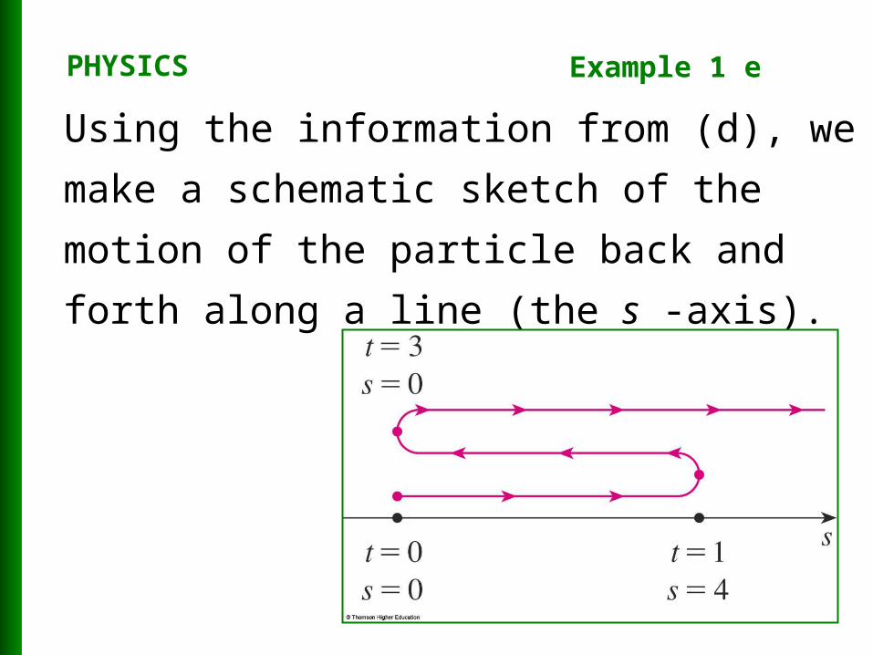
Using the information from (d), we make a
schematic sketch of the motion of the particle back
and forth along a line (the s -axis).
PHYSICS Example 1 e

Due to what we learned in (d) and (e), we need to
calculate the distances traveled during the time
intervals [0, 1], [1, 3], and [3, 5] separately.
PHYSICS Example 1 f

The distance traveled in the first second is:
|f(1) – f(0)| = |4 – 0| = 4 m
From t = 1 to t = 3, it is:
|f(3) – f(1)| = |0 – 4| = 4 m
From t = 3 to t = 5, it is:
|f(5) – f(3)| = |20 – 0| = 20 m
The total distance is 4 + 4 + 20 = 28 m
PHYSICS Example 1 f

The acceleration is the derivative of the velocity
function:
2
2
2
( ) 6 12
(4) 6(4) 12 12 /
d s dva t t
dt dt
a m s
PHYSICS Example 1 g

The figure shows the graphs of s, v, and a.
PHYSICS Example 1 h

The particle speeds up when the velocity is
positive and increasing (v and a are both positive)
and when the velocity is negative
and decreasing (v and a are both negative).
In other words, the particle speeds up when the velocity and acceleration have the same sign.
The particle is pushed in the same direction it is moving.
PHYSICS Example 1 i

From the figure, we see that this happens when 1 <
t < 2 and when t > 3.
PHYSICS Example 1 i

The particle slows down when v and a have
opposite signs, that is, when 0 ≤ t < 1 and when
2 < t < 3.
PHYSICS Example 1 i

This figure summarizes the motion of the particle.
PHYSICS Example 1 i

A current exists whenever electric charges move.
The figure shows part of a wire and electrons moving through a shaded plane surface.
PHYSICS Example 3

If ∆Q is the net charge that passes through this
surface during a time period ∆t, then the average
current during this time interval is defined as:
2 1
2 1
average current
Q QQ
t t t
PHYSICS Example 3

If we take the limit of this average current over
smaller and smaller time intervals, we get what is
called the current I at a given time t1:
Thus, the current is the rate at which charge flows through a surface.
It is measured in units of charge per unit time (often coulombs per second—called amperes).
0lim
t
Q dQI
t dt
PHYSICS Example 3

Velocity, density, and current are not the only rates
of change important in physics.
Others include: Power (the rate at which work is done) Rate of heat flow Temperature gradient (the rate of change of
temperature with respect to position)Rate of decay of a radioactive substance in
nuclear physics
PHYSICS

Let n = f (t) be the number of individuals in an
animal or plant population at time t.
The change in the population size between the times t = t1 and t = t2 is ∆n = f(t2) – f(t1)
BIOLOGY Example 6

AVERAGE RATE
So, the average rate of growth during the time
period t1 ≤ t ≤ t2 is:
2 1
2 1
( ) ( )average rate of growth
f t f tn
t t t

The instantaneous rate of growth is obtained from
this average rate of growth by letting the time
period ∆t approach 0:
0growth rate lim
t
n dn
t dt
Example 6INSTANTANEOUS RATE

Strictly speaking, this is not quite accurate.
This is because the actual graph of a population function n = f(t) would be a step function that is discontinuous whenever a birth or death occurs and, therefore, not differentiable.
BIOLOGY Example 6

However, for a large animal or plant population,
we can replace the graph by a smooth
approximating curve.
BIOLOGY Example 6

To be more specific, consider a population of
bacteria in a homogeneous nutrient medium.
Suppose that, by sampling the population at certain intervals, it is determined that the population doubles every hour.
BIOLOGY Example 6

If the initial population is n0 and the time t is
measured in hours, then
and, in general,
The population function is n = n02t
0
20
30
(1) 2 (0) 2
(2) 2 (1) 2
(3) 2 (2) 2
f f n
f f n
f f n
BIOLOGY Example 6
0( ) 2 tf t n
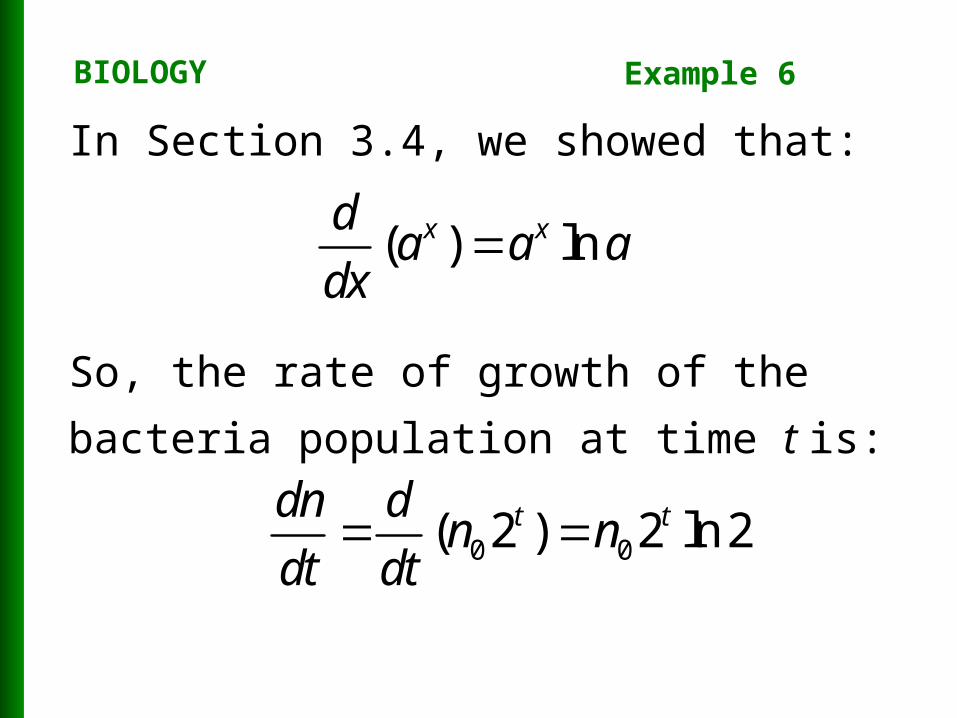
In Section 3.4, we showed that:
So, the rate of growth of the bacteria population at
time t is:
( ) lnx xda a a
dx
0 0( 2 ) 2 ln 2 t tdn dn n
dt dt
BIOLOGY Example 6

For example, suppose that we start with an initial
population of n0 = 100 bacteria.
Then, the rate of growth after 4 hours is:
This means that, after 4 hours, the bacteria population is growing at a rate of about 1109 bacteria per hour.
44 100 2 ln 2 1600ln 2 1109 t
dn
dt
BIOLOGY Example 6

ECONOMICS
Suppose C(x) is the total cost that a company
incurs in producing x units of a certain commodity.
The function C is called a cost function.
Example 8
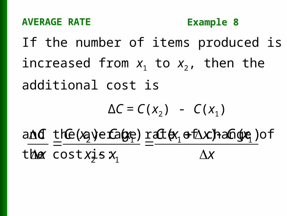
If the number of items produced is increased from
x1 to x2, then the additional cost is
∆C = C(x2) - C(x1)
and the average rate of change of the cost is:
2 1 1 1
2 1
( ) ( ) ( ) ( )
C x C x C x x C xC
x x x x
AVERAGE RATE Example 8

The limit of this quantity as ∆x → 0, that is, the
instantaneous rate of change of cost with respect to
the number of items produced, is called the
marginal cost by economists:
0marginal cost = lim
x
C dC
x dx
MARGINAL COST Example 8

As x often takes on only integer values, it may not
make literal sense to let ∆x approach 0.
However, we can always replace C(x) by a smooth approximating function—as in Example 6.
ECONOMICS Example 8

Taking ∆x = 1 and n large (so that ∆x is small
compared to n), we have:
C’(n) ≈ C(n + 1) – C(n)
Thus, the marginal cost of producing n units is approximately equal to the cost of producing one more unit [the (n + 1)st unit].
ECONOMICS Example 8

It is often appropriate to represent a total cost
function by a polynomial
C(x) = a + bx + cx2 + dx3
where a represents the overhead cost (rent, heat,
and maintenance) and the other terms represent the
cost of raw materials, labor, and so on.
ECONOMICS Example 8

The cost of raw materials may be proportional to x.
However, labor costs might depend partly on
higher powers of x because of overtime costs and
inefficiencies involved in large-scale operations.
ECONOMICS Example 8

For instance, suppose a company has estimated
that the cost (in dollars) of producing x items is:
C(x) = 10,000 + 5x + 0.01x2
Then, the marginal cost function is:
C’(x) = 5 + 0.02x
ECONOMICS Example 8
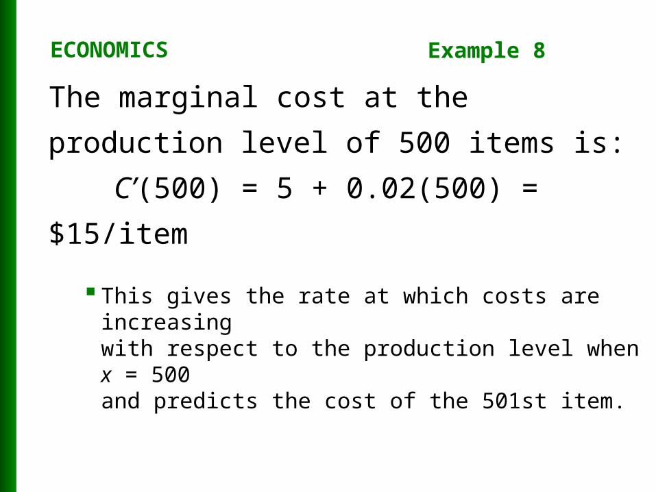
The marginal cost at the production level of 500
items is:
C’(500) = 5 + 0.02(500) = $15/item
This gives the rate at which costs are increasing with respect to the production level when x = 500 and predicts the cost of the 501st item.
ECONOMICS Example 8

The actual cost of producing the 501st item is:
C(501) – C(500) =
[10,000 + 5(501) + 0.01(501)2]
– [10,000 + 5(500) + 0.01(500)2]
=$15.01
Notice that C’(500) ≈ C(501) – C(500)
ECONOMICS Example 8

Economists also study marginal demand, marginal
revenue, and marginal profit, which are the
derivatives of the demand, revenue, and profit
functions.
These will be considered in Chapter 4—after we have developed techniques for finding the maximum and minimum values of functions.
ECONOMICS Example 8


![1 member(X,[Y| _ ] ) :- X = Y. member(X, [ _ | Y]) :- member(X, Y). It would be easier to write this…](https://static.documents.pub/doc/80x56/5a4d1c077f8b9ab0599f1b64/1-memberxy-x-y-memberx-y-memberx-y-it-would-be.jpg)


![Aarneel Profile Updated as on13.09 · Á Á Á X v o X } u &203$1< 352),/( ,1'(; ä ¾ / v } µ ] } v } µ h Y Y X Y Y Y Y Y Y Y Y Y Y Y Y X X í r î](https://static.documents.pub/doc/80x56/5f063de37e708231d417018e/aarneel-profile-updated-as-on1309-x-v-o-x-u-2031-352-1.jpg)


![> plot(cos(x) + sin(x), x=0..Pi); plot(tan(x), x=-Pi..Pi ... · > plot3d({sin(x*y), x + 2*y},x=-Pi..Pi,y=-Pi..Pi); ↵ c1:= [cos(x)-2*cos(0.4*y),sin(x)-2*sin(0.4*y),y]: ↵ c2:= [cos(x)+2*cos(0.4*y),sin(x)+2*sin(0.4*y),y]:](https://static.documents.pub/doc/80x56/5e87f19cd4429b02985e2e8b/-plotcosx-sinx-x0pi-plottanx-x-pipi-plot3dsinxy.jpg)

