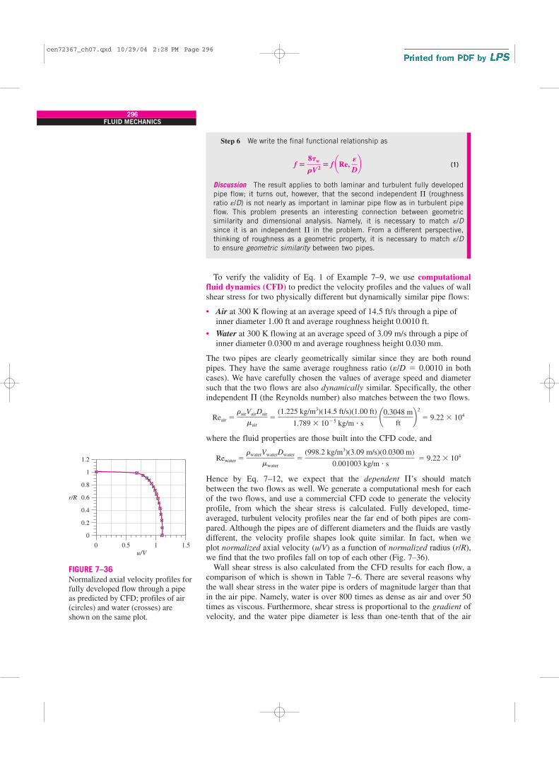
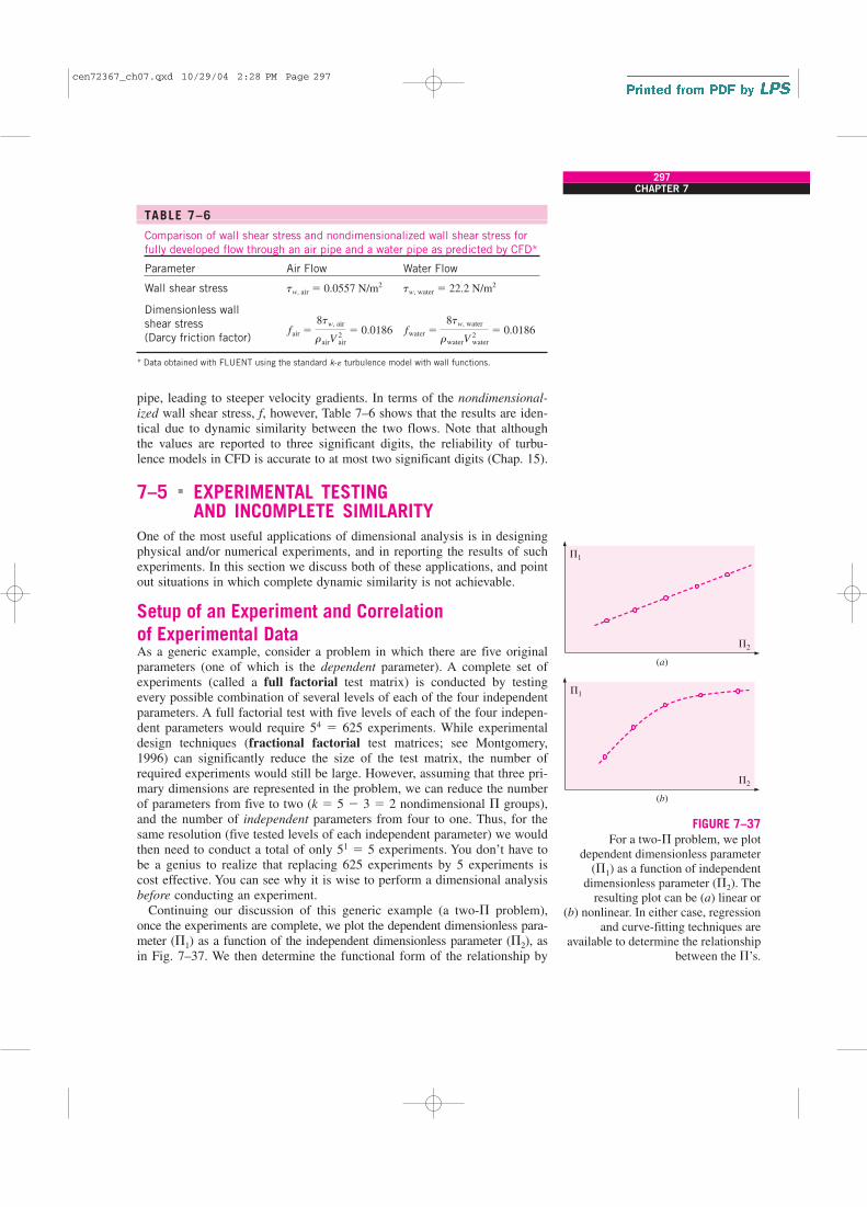
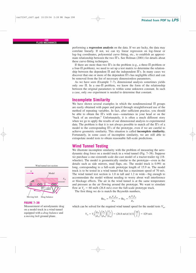
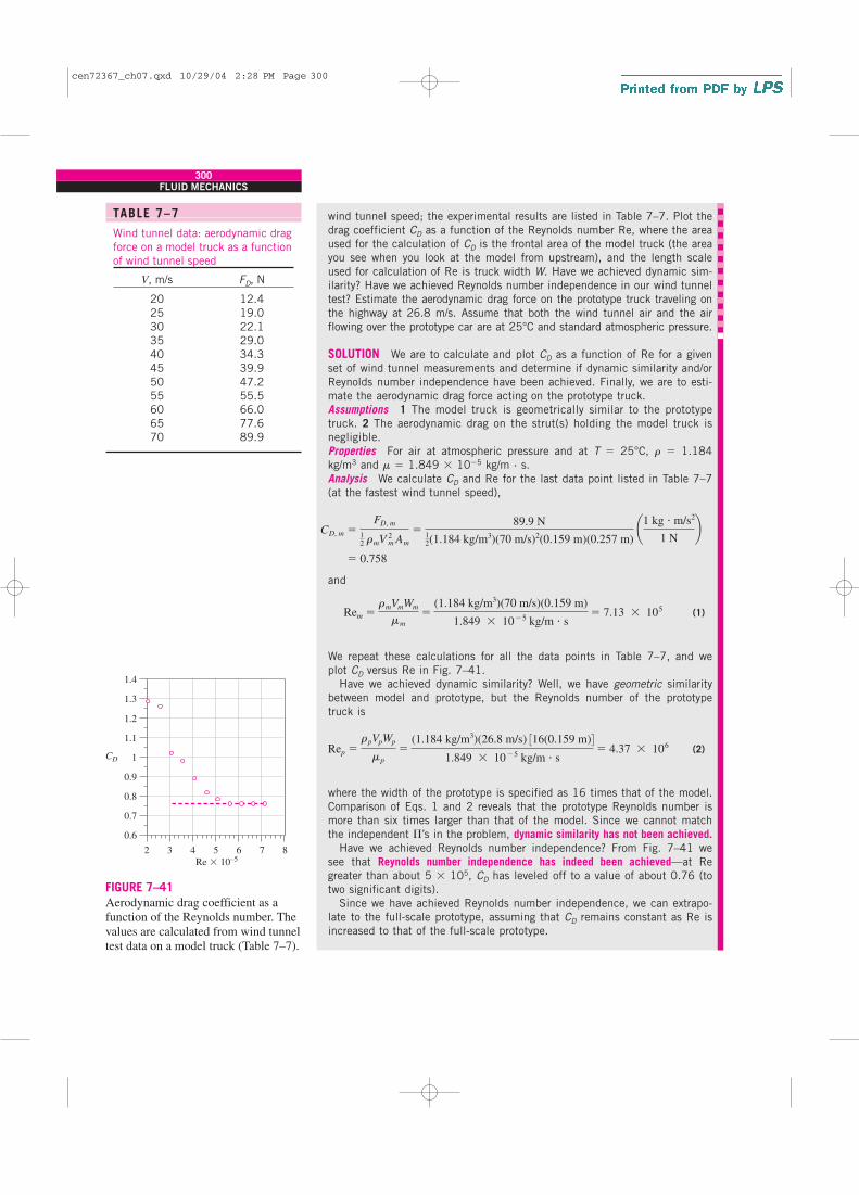
DIMENSIONAL ANALYSIS AND MODELING I n this chapter, we first review the concepts of dimensions and units. We then review the fundamental principle of dimensional homogeneity, and show how it is applied to equations in order to nondimensionalize them and to identify dimensionless groups. We discuss the concept of similarity between a model and a prototype. We also describe a powerful tool for engi- neers and scientists called dimensional analysis, in which the combination of dimensional variables, nondimensional variables, and dimensional con- stants into nondimensional parameters reduces the number of necessary independent parameters in a problem. We present a step-by-step method for obtaining these nondimensional parameters, called the method of repeating variables, which is based solely on the dimensions of the variables and con- stants. Finally, we apply this technique to several practical problems to illus- trate both its utility and its limitations. 269 CHAPTER 7 OBJECTIVES When you finish reading this chapter, you should be able to ■ Develop a better understanding of dimensions, units, and dimensional homogeneity of equations ■ Understand the numerous benefits of dimensional analysis ■ Know how to use the method of repeating variables to identify nondimensional parameters ■ Understand the concept of dynamic similarity and how to apply it to experimental modeling cen72367_ch07.qxd 10/29/04 2:27 PM Page 269
Transcript
D I M E N S I O N A L A N A LY S I SA N D M O D E L I N G
In this chapter, we first review the concepts of dimensions and units. We
then review the fundamental principle of dimensional homogeneity, and
show how it is applied to equations in order to nondimensionalize them
and to identify dimensionless groups. We discuss the concept of similarity
between a model and a prototype. We also describe a powerful tool for engi-
neers and scientists called dimensional analysis, in which the combination
of dimensional variables, nondimensional variables, and dimensional con-
stants into nondimensional parameters reduces the number of necessary
independent parameters in a problem. We present a step-by-step method for
obtaining these nondimensional parameters, called the method of repeating
variables, which is based solely on the dimensions of the variables and con-
stants. Finally, we apply this technique to several practical problems to illus-
trate both its utility and its limitations.
269
CHAPTER
7OBJECTIVES
When you finish reading this chapter, you
should be able to
� Develop a better understanding
of dimensions, units, and
dimensional homogeneity of
equations
� Understand the numerous
benefits of dimensional analysis
� Know how to use the method of
repeating variables to identify
nondimensional parameters
� Understand the concept of
dynamic similarity and how to
apply it to experimental
modeling
cen72367_ch07.qxd 10/29/04 2:27 PM Page 269
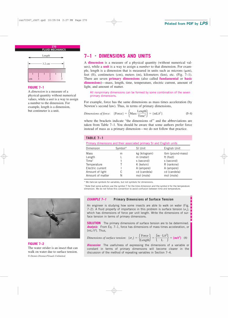
EXAMPLE 7–1 Primary Dimensions of Surface Tension
An engineer is studying how some insects are able to walk on water (Fig.
7–2). A fluid property of importance in this problem is surface tension (ss),
which has dimensions of force per unit length. Write the dimensions of sur-
face tension in terms of primary dimensions.
SOLUTION The primary dimensions of surface tension are to be determined.
Analysis From Eq. 7–1, force has dimensions of mass times acceleration, or
{mL/t2}. Thus,
Dimensions of surface tension: (1)
Discussion The usefulness of expressing the dimensions of a variable or
constant in terms of primary dimensions will become clearer in the
discussion of the method of repeating variables in Section 7–4.
{ss} � e Force
Lengthf � em � L/t2
Lf � {m/t2}
7–1 � DIMENSIONS AND UNITS
A dimension is a measure of a physical quantity (without numerical val-
ues), while a unit is a way to assign a number to that dimension. For exam-
ple, length is a dimension that is measured in units such as microns (�m),
There are seven primary dimensions (also called fundamental or basic
dimensions)—mass, length, time, temperature, electric current, amount of
light, and amount of matter.
All nonprimary dimensions can be formed by some combination of the sevenprimary dimensions.
For example, force has the same dimensions as mass times acceleration (by
Newton’s second law). Thus, in terms of primary dimensions,
Dimensions of force: (7–1)
where the brackets indicate “the dimensions of” and the abbreviations are
taken from Table 7–1. You should be aware that some authors prefer force
instead of mass as a primary dimension—we do not follow that practice.
{Force} � eMass Length
Time2f � {mL/t2}
270FLUID MECHANICS
3.2 cm
1 2 3cm
Length
FIGURE 7–1
A dimension is a measure of a
physical quantity without numerical
values, while a unit is a way to assign
a number to the dimension. For
example, length is a dimension,
but centimeter is a unit.
TABLE 7–1
Primary dimensions and their associated primary SI and English units
Dimension Symbol* SI Unit English Unit
Mass m kg (kilogram) lbm (pound-mass)
Length L m (meter) ft (foot)
Time† t s (second) s (second)
Temperature T K (kelvin) R (rankine)
Electric current I A (ampere) A (ampere)
Amount of light C cd (candela) cd (candela)
Amount of matter N mol (mole) mol (mole)
* We italicize symbols for variables, but not symbols for dimensions.
† Note that some authors use the symbol T for the time dimension and the symbol u for the temperaturedimension. We do not follow this convention to avoid confusion between time and temperature.
g = gravitationalacceleration in thenegative z-direction
FIGURE 7–8
Object falling in a vacuum. Vertical
velocity is drawn positively, so w 0
for a falling object.
L
P0
V, P∞
FIGURE 7–9
In a typical fluid flow problem, the
scaling parameters usually include a
characteristic length L, a characteristic
velocity V, and a reference pressure
difference P0 � P�. Other parameters
and fluid properties such as density,
viscosity, and gravitational
acceleration enter the problem
as well.
cen72367_ch07.qxd 10/29/04 2:27 PM Page 273
Substitution of Eq. 7–6 into Eq. 7–4 gives
(7–7)
which is the desired nondimensional equation. The grouping of dimensional
constants in Eq. 7–7 is the square of a well-known nondimensional para-
meter or dimensionless group called the Froude number,
Froude number: (7–8)
The Froude number also appears as a nondimensional parameter in free-
surface flows (Chap. 13), and can be thought of as the ratio of inertial force
to gravitational force (Fig. 7–10). You should note that in some older
textbooks, Fr is defined as the square of the parameter shown in Eq. 7–8.
Substitution of Eq. 7–8 into Eq. 7–7 yields
Nondimensionalized equation of motion: (7–9)
In dimensionless form, only one parameter remains, namely the Froude
number. Equation 7–9 is easily solved by integrating twice and applying the
initial conditions. The result is an expression for dimensionless elevation z*
at any dimensionless time t*:
Nondimensional result: (7–10)
Comparison of Eqs. 7–5 and 7–10 reveals that they are equivalent. In fact,
for practice, substitute Eqs. 7–6 and 7–8 into Eq. 7–5 to verify Eq. 7–10.
It seems that we went through a lot of extra algebra to generate the same
final result. What then is the advantage of nondimensionalizing the equa-
tion? Before answering this question, we note that the advantages are not so
clear in this simple example because we were able to analytically integrate
the differential equation of motion. In more complicated problems, the dif-
ferential equation (or more generally the coupled set of differential equa-
tions) cannot be integrated analytically, and engineers must either integrate
the equations numerically, or design and conduct physical experiments to
obtain the needed results, both of which can incur considerable time and
expense. In such cases, the nondimensional parameters generated by nondi-
mensionalizing the equations are extremely useful and can save much effort
and expense in the long run.
There are two key advantages of nondimensionalization (Fig. 7–11). First,
it increases our insight about the relationships between key parameters.
Equation 7–8 reveals, for example, that doubling w0 has the same effect as
decreasing z0 by a factor of 4. Second, it reduces the number of parameters
in the problem. For example, the original problem contains one dependent
variable, z; one independent variable, t; and three additional dimensional
constants, g, w0, and z0. The nondimensionalized problem contains one
dependent parameter, z*; one independent parameter, t*; and only one
additional parameter, namely the dimensionless Froude number, Fr. The
number of additional parameters has been reduced from three to one!
Example 7–3 further illustrates the advantages of nondimensionalization.
z* � 1 � t* � 1
2Fr2 t*2
d 2z*
dt*2� �
1
Fr2
Fr �w0
2gz0
d 2z
dt 2�
d 2(z0z*)
d(z0t*/w0)2
�w 2
0
z0
d 2z*
dt*2� �g →
w 20
gz0
d 2z*
dt*2� �1
274FLUID MECHANICS
Sluicegate
y1
V1
2Vy2
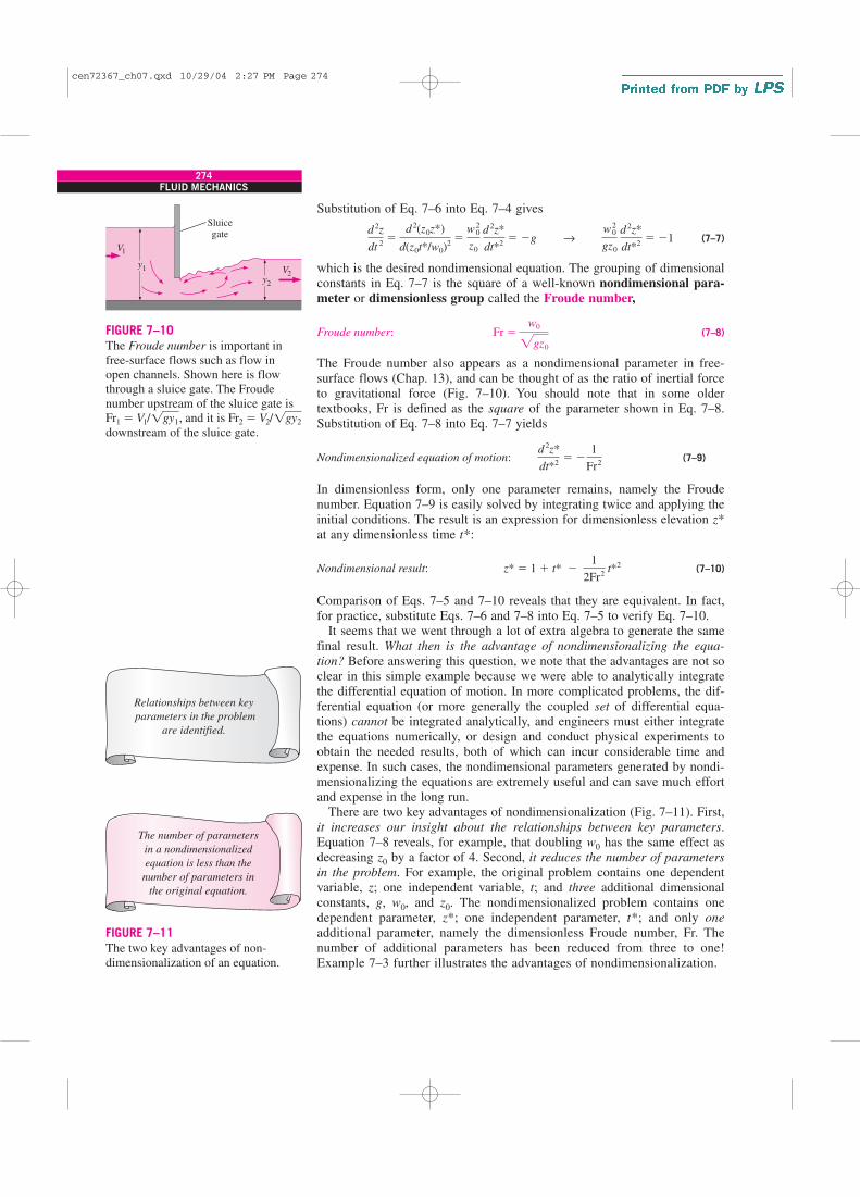
FIGURE 7–10
The Froude number is important in
free-surface flows such as flow in
open channels. Shown here is flow
through a sluice gate. The Froude
number upstream of the sluice gate is
and it is
downstream of the sluice gate.
Fr2 � V2/1gy2Fr1 � V1/1gy1,
Relationships between key
parameters in the problem
are identified.
The number of parameters
in a nondimensionalized
equation is less than the
number of parameters in
the original equation.
FIGURE 7–11
The two key advantages of non-
dimensionalization of an equation.
cen72367_ch07.qxd 10/29/04 2:27 PM Page 274
EXAMPLE 7–3 Illustration of the Advantages
of Nondimensionalization
Your little brother’s high school physics class conducts experiments in a
large vertical pipe whose inside is kept under vacuum conditions. The stu-
dents are able to remotely release a steel ball at initial height z0 between 0
and 15 m (measured from the bottom of the pipe), and with initial vertical
speed w0 between 0 and 10 m/s. A computer coupled to a network of photo-
sensors along the pipe enables students to plot the trajectory of the steel
ball (height z plotted as a function of time t) for each test. The students are
unfamiliar with dimensional analysis or nondimensionalization techniques,
and therefore conduct several “brute force” experiments to determine how
the trajectory is affected by initial conditions z0 and w0. First they hold w0
fixed at 4 m/s and conduct experiments at five different values of z0: 3, 6,
9, 12, and 15 m. The experimental results are shown in Fig. 7–12a. Next,
they hold z0 fixed at 10 m and conduct experiments at five different values
of w0: 2, 4, 6, 8, and 10 m/s. These results are shown in Fig. 7–12b. Later
that evening, your brother shows you the data and the trajectory plots and
tells you that they plan to conduct more experiments at different values of z0
and w0. You explain to him that by first nondimensionalizing the data, the
problem can be reduced to just one parameter, and no further experiments
are required. Prepare a nondimensional plot to prove your point and discuss.
SOLUTION A nondimensional plot is to be generated from all the available
trajectory data. Specifically, we are to plot z* as a function of t*.
Assumptions The inside of the pipe is subjected to strong enough vacuum
pressure that aerodynamic drag on the ball is negligible.
Properties The gravitational constant is 9.81 m/s2.
Analysis Equation 7–4 is valid for this problem, as is the nondimensional-
ization that resulted in Eq. 7–9. As previously discussed, this problem com-
bines three of the original dimensional parameters (g, z0, and w0) into one
nondimensional parameter, the Froude number. After converting to the
dimensionless variables of Eq. 7–6, the 10 trajectories of Fig. 7–12a and b
are replotted in dimensionless format in Fig. 7–13. It is clear that all the
trajectories are of the same family, with the Froude number as the only
remaining parameter. Fr2 varies from about 0.041 to about 1.0 in these exper-
iments. If any more experiments are to be conducted, they should include
combinations of z0 and w0 that produce Froude numbers outside of this range.
A large number of additional experiments would be unnecessary, since all the
trajectories would be of the same family as those plotted in Fig. 7–13.
Discussion At low Froude numbers, gravitational forces are much larger than
inertial forces, and the ball falls to the floor in a relatively short time. At large
values of Fr on the other hand, inertial forces dominate initially, and the ball
rises a significant distance before falling; it takes much longer for the ball to
hit the ground. The students are obviously not able to adjust the gravitational
constant, but if they could, the brute force method would require many more
experiments to document the effect of g. If they nondimensionalize first, how-
ever, the dimensionless trajectory plots already obtained and shown in Fig.
7–13 would be valid for any value of g; no further experiments would be
required unless Fr were outside the range of tested values.
If you are still not convinced that nondimensionalizing the equations and the
parameters has many advantages, consider this: In order to reasonably docu-
ment the trajectories of Example 7–3 for a range of all three of the dimensional
275CHAPTER 7
(b)
z0 = 10 m
z, m
0
0 0.5 1 1.5 2
t, s
2.5 3
2
4
6
8
10
12
14
16
10 m/s
w0 =
8 m/s
6 m/s
4 m/s
2 m/s
FIGURE 7–12
Trajectories of a steel ball falling in
a vacuum: (a) w0 fixed at 4 m/s, and
(b) z0 fixed at 10 m (Example 7–3).
Fr2
Fr2 = 1.0
z*
0
0 0.5 1 1.5 2
t*
2.5 3
0.2
0.4
0.6
0.8
1
1.2
1.4
1.6
Fr2 = 0.041
FIGURE 7–13
Trajectories of a steel ball falling
in a vacuum. Data of Fig. 7–12a
and b are nondimensionalized and
combined onto one plot.
(a)
z, m
0
0 0.5 1 1.5 2
t, s
2.5 3
2
4
6
8
10
12
14
16
15 mz0 =
wo = 4 m/s
12 m
9 m
6 m
3 m
cen72367_ch07.qxd 10/29/04 2:27 PM Page 275
parameters g, z0, and w0, the brute force method would require several (say a
minimum of four) additional plots like Fig. 7–12a at various values (levels) of
w0, plus several additional sets of such plots for a range of g. A complete data
set for three parameters with five levels of each parameter would require 53 �125 experiments! Nondimensionalization reduces the number of parameters
from three to one—a total of only 51 � 5 experiments are required for the
same resolution. (For five levels, only five dimensionless trajectories like those
of Fig. 7–13 are required, at carefully chosen values of Fr.)
Another advantage of nondimensionalization is that extrapolation to
untested values of one or more of the dimensional parameters is possible.
For example, the data of Example 7–3 were taken at only one value of grav-
itational acceleration. Suppose you wanted to extrapolate these data to a dif-
ferent value of g. Example 7–4 shows how this is easily accomplished via
the dimensionless data.
EXAMPLE 7–4 Extrapolation of Nondimensionalized Data
The gravitational constant at the surface of the moon is only about one-sixth
of that on earth. An astronaut on the moon throws a baseball at an initial
speed of 21.0 m/s at a 5° angle above the horizon and at 2.0 m above the
moon’s surface (Fig. 7–14). (a) Using the dimensionless data of Example
7–3 shown in Fig. 7–13, predict how long it takes for the baseball to fall to
the ground. (b) Do an exact calculation and compare the result to that of
part (a).
SOLUTION Experimental data obtained on earth are to be used to predict
the time required for a baseball to fall to the ground on the moon.
Assumptions 1 The horizontal velocity of the baseball is irrelevant. 2 The
surface of the moon is perfectly flat near the astronaut. 3 There is no aero-
dynamic drag on the ball since there is no atmosphere on the moon. 4 Moon
gravity is one-sixth that of earth.
Properties The gravitational constant on the moon is gmoon ≅ 9.81/6
� 1.63 m/s2.
Analysis (a) The Froude number is calculated based on the value of gmoon
and the vertical component of initial speed,
from which
This value of Fr2 is nearly the same as the largest value plotted in Fig.
7–13. Thus, in terms of dimensionless variables, the baseball strikes the
ground at t* ≅ 2.75, as determined from Fig. 7–13. Converting back to
dimensional variables using Eq. 7–6,
Estimated time to strike the ground:
(b) An exact calculation is obtained by setting z equal to zero in Eq. 7–5
and solving for time t (using the quadratic formula),
t �t*z0
w0
�2.75(2.0 m)
1.830 m/s� 3.01 s
Fr2 �w 2
0
gmoonz0
�(1.830 m/s)2
(1.63 m/s2)(2.0 m)� 1.03
w0 � (21.0 m/s) sin(5) � 1.830 m/s
276FLUID MECHANICS
FIGURE 7–14
Throwing a baseball on the moon
(Example 7–4).
cen72367_ch07.qxd 10/29/04 2:27 PM Page 276
Exact time to strike the ground:
Discussion If the Froude number had landed between two of the trajecto-
ries of Fig. 7–13, interpolation would have been required. Since some of
the numbers are precise to only two significant digits, the small difference
between the results of part (a) and part (b) is of no concern. The final result
is t � 3.0 s to two significant digits.
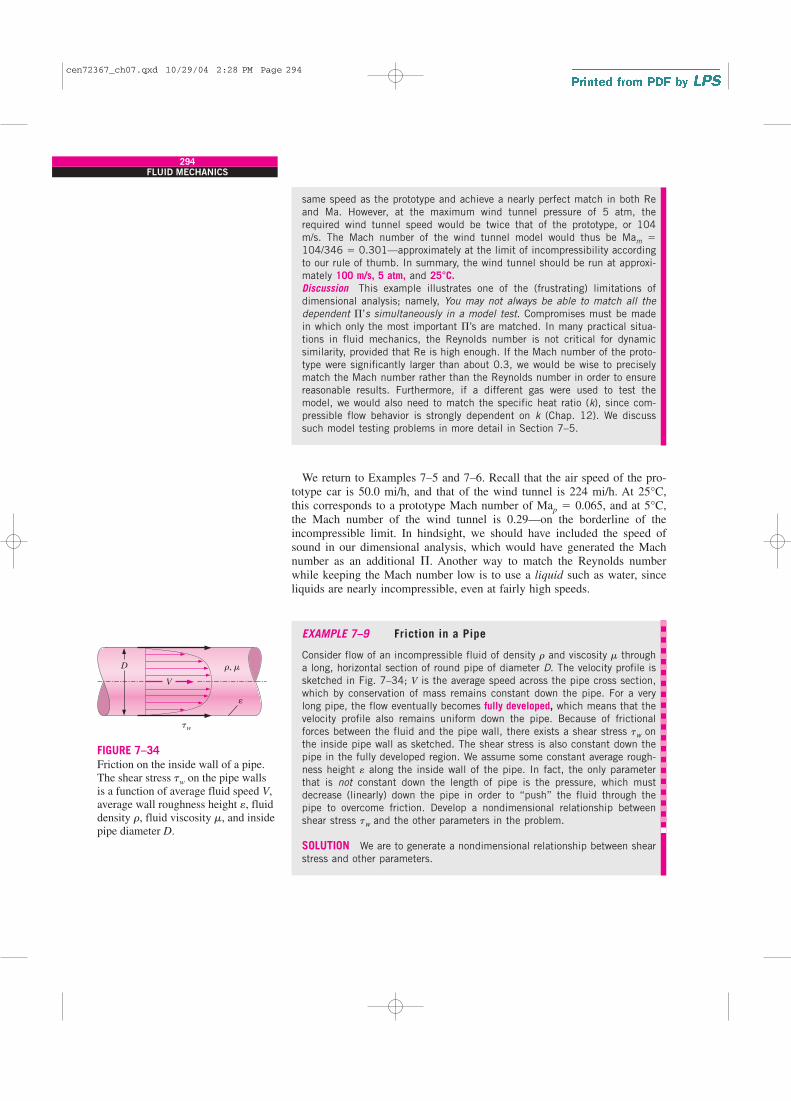
The differential equations of motion for fluid flow are derived and dis-
cussed in Chap. 9. In Chap. 10 you will find an analysis similar to that pre-
sented here, but applied to the differential equations for fluid flow. It turns
out that the Froude number also appears in that analysis, as do three other
important dimensionless parameters—the Reynolds number, Euler number,
and Strouhal number (Fig. 7–15).
7–3 � DIMENSIONAL ANALYSIS AND SIMILARITY
Nondimensionalization of an equation by inspectional analysis is useful
only when one knows the equation to begin with. However, in many cases
in real-life engineering, the equations are either not known or too difficult to
solve; oftentimes experimentation is the only method of obtaining reliable
information. In most experiments, to save time and money, tests are per-
formed on a geometrically scaled model, rather than on the full-scale proto-
type. In such cases, care must be taken to properly scale the results. We
introduce here a powerful technique called dimensional analysis. While
typically taught in fluid mechanics, dimensional analysis is useful in all dis-
ciplines, especially when it is necessary to design and conduct experiments.
You are encouraged to use this powerful tool in other subjects as well, not just
in fluid mechanics. The three primary purposes of dimensional analysis are
• To generate nondimensional parameters that help in the design of
experiments (physical and/or numerical) and in the reporting of
experimental results
• To obtain scaling laws so that prototype performance can be predicted
from model performance
• To (sometimes) predict trends in the relationship between parameters
Before discussing the technique of dimensional analysis, we first explain
the underlying concept of dimensional analysis—the principle of similarity.
There are three necessary conditions for complete similarity between a
model and a prototype. The first condition is geometric similarity—the
model must be the same shape as the prototype, but may be scaled by some
constant scale factor. The second condition is kinematic similarity, which
means that the velocity at any point in the model flow must be proportional
�1.830 m/s � 2(1.830 m/s)2 � 2(2.0 m)(1.63 m/s2)
1.63 m/s2� 3.05 s
t �w0 � 2w 2
0 � 2z0g
g
277CHAPTER 7
r, m
gP
∞
P0
L
f V
Re =rVL
m
St =fL
VEu =
P0 – P∞
rV2
Fr =V
gL
FIGURE 7–15
In a general unsteady fluid flow
problem with a free surface, the
scaling parameters include a
characteristic length L,
a characteristic velocity V, a
characteristic frequency f, and a
reference pressure difference
P0 � P�. Nondimensionalization of
the differential equations of fluid flow
produces four dimensionless
parameters: the Reynolds number,
Froude number, Strouhal number,
and Euler number (see Chap. 10).
cen72367_ch07.qxd 10/29/04 2:27 PM Page 277
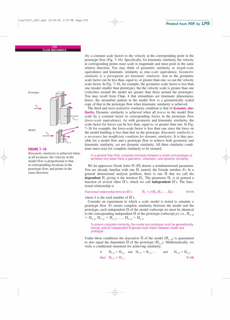
(by a constant scale factor) to the velocity at the corresponding point in the
prototype flow (Fig. 7–16). Specifically, for kinematic similarity the velocity
at corresponding points must scale in magnitude and must point in the same
relative direction. You may think of geometric similarity as length-scale
equivalence and kinematic similarity as time-scale equivalence. Geometric
similarity is a prerequisite for kinematic similarity. Just as the geometric
scale factor can be less than, equal to, or greater than one, so can the velocity
scale factor. In Fig. 7–16, for example, the geometric scale factor is less than
one (model smaller than prototype), but the velocity scale is greater than one
(velocities around the model are greater than those around the prototype).
You may recall from Chap. 4 that streamlines are kinematic phenomena;
hence, the streamline pattern in the model flow is a geometrically scaled
copy of that in the prototype flow when kinematic similarity is achieved.
The third and most restrictive similarity condition is that of dynamic sim-
ilarity. Dynamic similarity is achieved when all forces in the model flow
scale by a constant factor to corresponding forces in the prototype flow
(force-scale equivalence). As with geometric and kinematic similarity, the
scale factor for forces can be less than, equal to, or greater than one. In Fig.
7–16 for example, the force-scale factor is less than one since the force on
the model building is less than that on the prototype. Kinematic similarity is
a necessary but insufficient condition for dynamic similarity. It is thus pos-
sible for a model flow and a prototype flow to achieve both geometric and
kinematic similarity, yet not dynamic similarity. All three similarity condi-
tions must exist for complete similarity to be ensured.
In a general flow field, complete similarity between a model and prototype isachieved only when there is geometric, kinematic, and dynamic similarity.
We let uppercase Greek letter Pi (�) denote a nondimensional parameter.
You are already familiar with one �, namely the Froude number, Fr. In a
general dimensional analysis problem, there is one � that we call the
dependent �, giving it the notation �1. The parameter �1 is in general a
function of several other �’s, which we call independent �’s. The func-
tional relationship is
Functional relationship between �’s: (7–11)
where k is the total number of �’s.
Consider an experiment in which a scale model is tested to simulate a
prototype flow. To ensure complete similarity between the model and the
prototype, each independent � of the model (subscript m) must be identical
to the corresponding independent � of the prototype (subscript p), i.e., �2, m
� �2, p, �3, m � �3, p, . . . , �k, m � �k, p.
To ensure complete similarity, the model and prototype must be geometricallysimilar, and all independent � groups must match between model andprototype.
Under these conditions the dependent � of the model (�1, m) is guaranteed
to also equal the dependent � of the prototype (�1, p). Mathematically, we
write a conditional statement for achieving similarity,
(7–12) then �1, m � �1, p
If �2, m � �2, p and �3, m � �3, p p and �k, m � �k, p,
�1 � f (�2, �3, p , �k)
278FLUID MECHANICS
Prototype:
Model:
Vp
Vm
FD, m
FD, p
FIGURE 7–16
Kinematic similarity is achieved when,
at all locations, the velocity in the
model flow is proportional to that
at corresponding locations in the
prototype flow, and points in the
same direction.
cen72367_ch07.qxd 10/29/04 2:27 PM Page 278
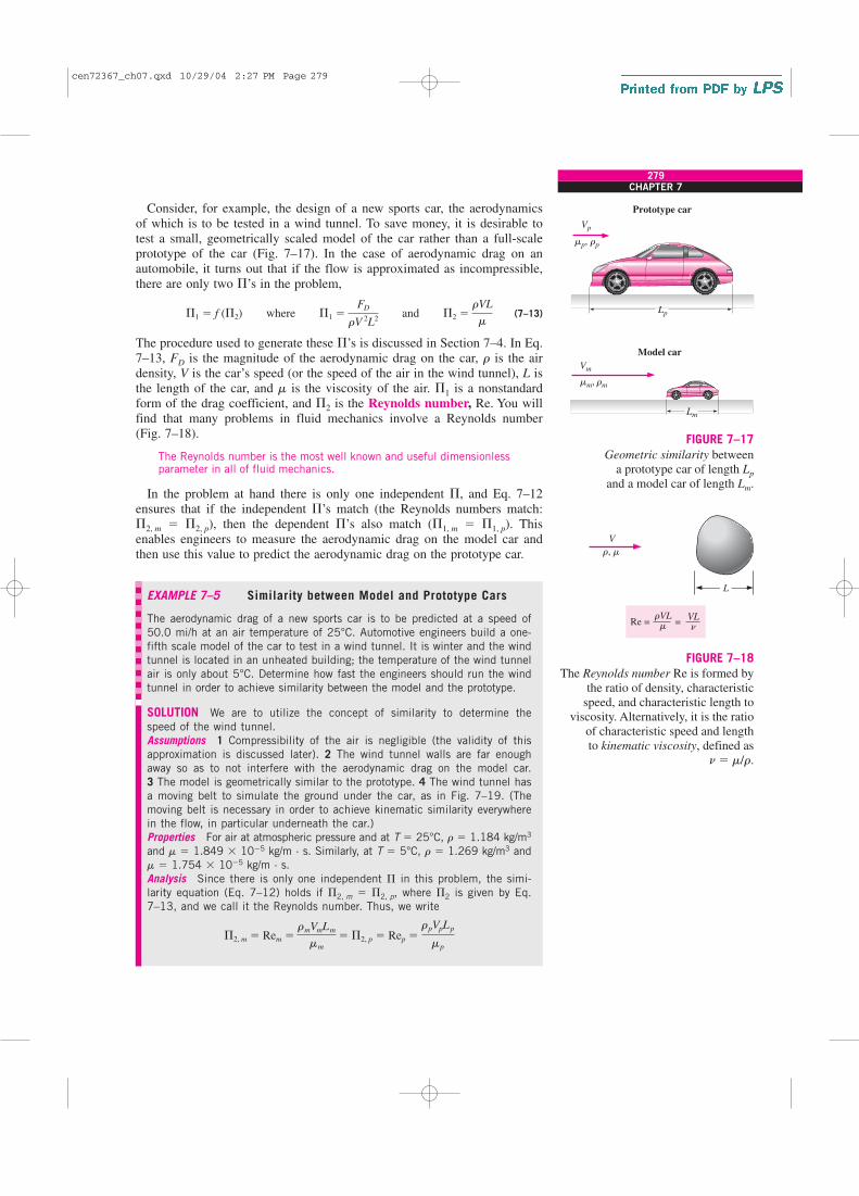
Consider, for example, the design of a new sports car, the aerodynamics
of which is to be tested in a wind tunnel. To save money, it is desirable to
test a small, geometrically scaled model of the car rather than a full-scale
prototype of the car (Fig. 7–17). In the case of aerodynamic drag on an
automobile, it turns out that if the flow is approximated as incompressible,
there are only two �’s in the problem,
(7–13)
The procedure used to generate these �’s is discussed in Section 7–4. In Eq.
7–13, FD is the magnitude of the aerodynamic drag on the car, r is the air
density, V is the car’s speed (or the speed of the air in the wind tunnel), L is
the length of the car, and m is the viscosity of the air. �1 is a nonstandard
form of the drag coefficient, and �2 is the Reynolds number, Re. You will
find that many problems in fluid mechanics involve a Reynolds number
(Fig. 7–18).
The Reynolds number is the most well known and useful dimensionlessparameter in all of fluid mechanics.
In the problem at hand there is only one independent �, and Eq. 7–12
ensures that if the independent �’s match (the Reynolds numbers match:
�2, m � �2, p), then the dependent �’s also match (�1, m � �1, p). This
enables engineers to measure the aerodynamic drag on the model car and
then use this value to predict the aerodynamic drag on the prototype car.
EXAMPLE 7–5 Similarity between Model and Prototype Cars
The aerodynamic drag of a new sports car is to be predicted at a speed of
50.0 mi/h at an air temperature of 25°C. Automotive engineers build a one-
fifth scale model of the car to test in a wind tunnel. It is winter and the wind
tunnel is located in an unheated building; the temperature of the wind tunnel
air is only about 5°C. Determine how fast the engineers should run the wind
tunnel in order to achieve similarity between the model and the prototype.
SOLUTION We are to utilize the concept of similarity to determine the
speed of the wind tunnel.
Assumptions 1 Compressibility of the air is negligible (the validity of this
approximation is discussed later). 2 The wind tunnel walls are far enough
away so as to not interfere with the aerodynamic drag on the model car.
3 The model is geometrically similar to the prototype. 4 The wind tunnel has
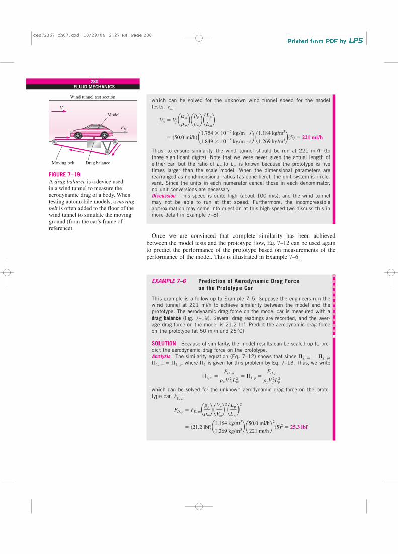
a moving belt to simulate the ground under the car, as in Fig. 7–19. (The
moving belt is necessary in order to achieve kinematic similarity everywhere
in the flow, in particular underneath the car.)
Properties For air at atmospheric pressure and at T � 25°C, r � 1.184 kg/m3
and m � 1.849 � 10�5 kg/m · s. Similarly, at T � 5°C, r � 1.269 kg/m3 and
m � 1.754 � 10�5 kg/m · s.
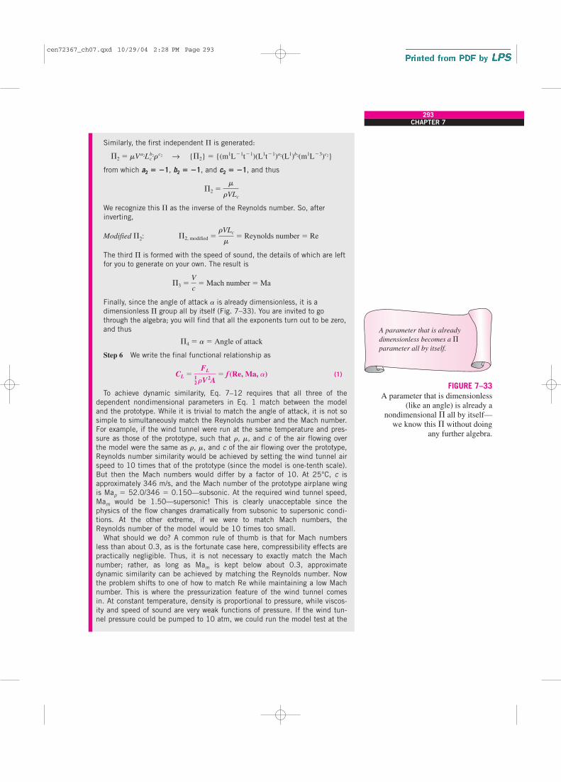
Analysis Since there is only one independent � in this problem, the simi-
larity equation (Eq. 7–12) holds if �2, m � �2, p, where �2 is given by Eq.
7–13, and we call it the Reynolds number. Thus, we write
�2, m � Rem �rmVmLm
mm
� �2, p � Rep �rpVpLp
mp
�1 � f (�2) where �1 �FD
rV 2L2 and �2 �
rVL
m
279CHAPTER 7
Prototype car
Model car
Vp
mp, rp
Lp
Vm
mm, rm
Lm
FIGURE 7–17
Geometric similarity between
a prototype car of length Lp
and a model car of length Lm.
Re = = rVLm
r, m
VLn
V
L
FIGURE 7–18
The Reynolds number Re is formed by
the ratio of density, characteristic
speed, and characteristic length to
viscosity. Alternatively, it is the ratio
of characteristic speed and length
to kinematic viscosity, defined as
n� m/r.
cen72367_ch07.qxd 10/29/04 2:27 PM Page 279
which can be solved for the unknown wind tunnel speed for the model
tests, Vm,
Thus, to ensure similarity, the wind tunnel should be run at 221 mi/h (to
three significant digits). Note that we were never given the actual length of
either car, but the ratio of Lp to Lm is known because the prototype is five
times larger than the scale model. When the dimensional parameters are
rearranged as nondimensional ratios (as done here), the unit system is irrele-
vant. Since the units in each numerator cancel those in each denominator,
no unit conversions are necessary.
Discussion This speed is quite high (about 100 m/s), and the wind tunnel
may not be able to run at that speed. Furthermore, the incompressible
approximation may come into question at this high speed (we discuss this in
more detail in Example 7–8).
Once we are convinced that complete similarity has been achieved
between the model tests and the prototype flow, Eq. 7–12 can be used again
to predict the performance of the prototype based on measurements of the
performance of the model. This is illustrated in Example 7–6.
EXAMPLE 7–6 Prediction of Aerodynamic Drag Force
on the Prototype Car
This example is a follow-up to Example 7–5. Suppose the engineers run the
wind tunnel at 221 mi/h to achieve similarity between the model and the
prototype. The aerodynamic drag force on the model car is measured with a
drag balance (Fig. 7–19). Several drag readings are recorded, and the aver-
age drag force on the model is 21.2 lbf. Predict the aerodynamic drag force
on the prototype (at 50 mi/h and 25°C).
SOLUTION Because of similarity, the model results can be scaled up to pre-
dict the aerodynamic drag force on the prototype.
Analysis The similarity equation (Eq. 7–12) shows that since �2, m � �2, p,
�1, m � �1, p, where �1 is given for this problem by Eq. 7–13. Thus, we write
which can be solved for the unknown aerodynamic drag force on the proto-
type car, FD, p,
� (21.2 lbf)a1.184 kg/m3
1.269 kg/m3b a50.0 mi/h
221 mi/hb 2
(5)2 � 25.3 lbf
FD, p � FD, marp
rm
b aVp
Vm
b 2aLp
Lm
b 2
�1, m �FD, m
rmV 2mL2
m
� �1, p �FD, p
rpV2pL2
p
� (50.0 mi/h)˛a1.754 � 10�5 kg/m � s
1.849 � 10�5 kg/m � sb ˛a1.184 kg/m3
1.269 kg/m3b (5) � 221 mi/h
Vm � Vpamm
mp
b arp
rm
b aLp
Lm
b
280FLUID MECHANICS
Model
Moving belt
Wind tunnel test section
Drag balance
FD
V
FIGURE 7–19
A drag balance is a device used
in a wind tunnel to measure the
aerodynamic drag of a body. When
testing automobile models, a moving
belt is often added to the floor of the
wind tunnel to simulate the moving
ground (from the car’s frame of
reference).
cen72367_ch07.qxd 10/29/04 2:27 PM Page 280
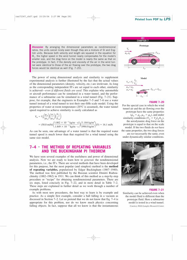
Discussion By arranging the dimensional parameters as nondimensional
ratios, the units cancel nicely even though they are a mixture of SI and Eng-
lish units. Because both velocity and length are squared in the equation for
�1, the higher speed in the wind tunnel nearly compensates for the model’s
smaller size, and the drag force on the model is nearly the same as that on
the prototype. In fact, if the density and viscosity of the air in the wind tun-
nel were identical to those of the air flowing over the prototype, the two drag
forces would be identical as well (Fig. 7–20).
The power of using dimensional analysis and similarity to supplement
experimental analysis is further illustrated by the fact that the actual values
of the dimensional parameters (density, velocity, etc.) are irrelevant. As long
as the corresponding independent �’s are set equal to each other, similarity
is achieved—even if different fluids are used. This explains why automobile
or aircraft performance can be simulated in a water tunnel, and the perfor-
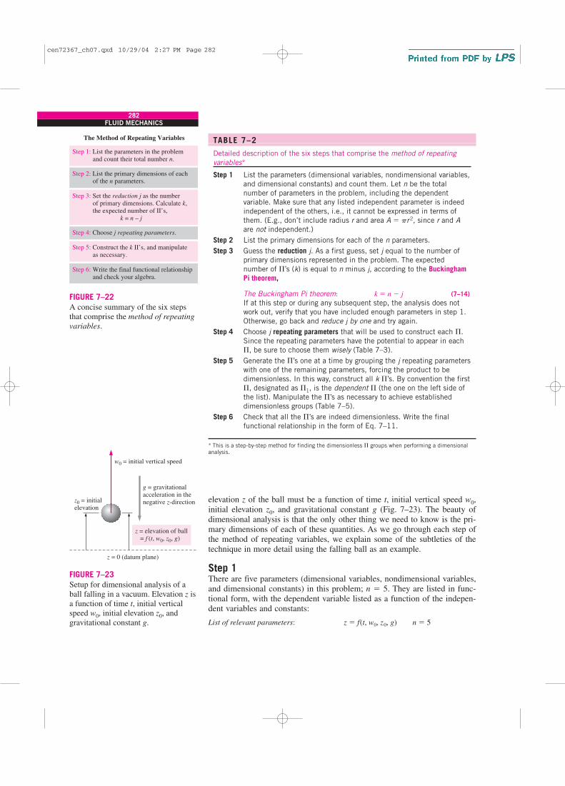
mance of a submarine can be simulated in a wind tunnel (Fig. 7–21). Sup-
pose, for example, that the engineers in Examples 7–5 and 7–6 use a water
tunnel instead of a wind tunnel to test their one-fifth scale model. Using the
properties of water at room temperature (20°C is assumed), the water tunnel
speed required to achieve similarity is easily calculated as
As can be seen, one advantage of a water tunnel is that the required water
tunnel speed is much lower than that required for a wind tunnel using the
same size model.
7–4 � THE METHOD OF REPEATING VARIABLESAND THE BUCKINGHAM PI THEOREM
We have seen several examples of the usefulness and power of dimensional
analysis. Now we are ready to learn how to generate the nondimensional
parameters, i.e., the �’s. There are several methods that have been developed
for this purpose, but the most popular (and simplest) method is the method
of repeating variables, popularized by Edgar Buckingham (1867–1940).
The method was first published by the Russian scientist Dimitri Riabou-
chinsky (1882–1962) in 1911. We can think of this method as a step-by-step
procedure or “recipe” for obtaining nondimensional parameters. There are
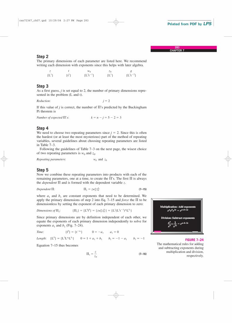
six steps, listed concisely in Fig. 7–22, and in more detail in Table 7–2.
These steps are explained in further detail as we work through a number of
example problems.
As with most new procedures, the best way to learn is by example and
practice. As a simple first example, consider a ball falling in a vacuum as
discussed in Section 7–2. Let us pretend that we do not know that Eq. 7–4 is
appropriate for this problem, nor do we know much physics concerning
falling objects. In fact, suppose that all we know is that the instantaneous
� (50.0 mi/h)a1.002 � 10�3 kg/m � s)
1.849 � 10�5 kg/m � sb a1.184 kg/m3
998.0 kg/m3b (5) � 16.1 mi/h
Vm � Vpamm
mp
b arp
rm
b aLp
Lm
b
281CHAPTER 7
FIGURE 7–21
Similarity can be achieved even when
the model fluid is different than the
prototype fluid. Here a submarine
model is tested in a wind tunnel.
Courtesy NASA Langley Research Center.
Prototype
Model
Vp
mp, rpFD, p
Lp
Vm = Vp
mm = mp
rm = rpFD, m = FD, p
Lm
Lp
Lm
FIGURE 7–20
For the special case in which the wind
tunnel air and the air flowing over the
prototype have the same properties
(rm � rp, mm � mp), and under
similarity conditions (Vm � VpLp/Lm),
the aerodynamic drag force on the
prototype is equal to that on the scale
model. If the two fluids do not have
the same properties, the two drag forces
are not necessarily the same, even
under dynamically similar conditions.
cen72367_ch07.qxd 10/29/04 2:27 PM Page 281
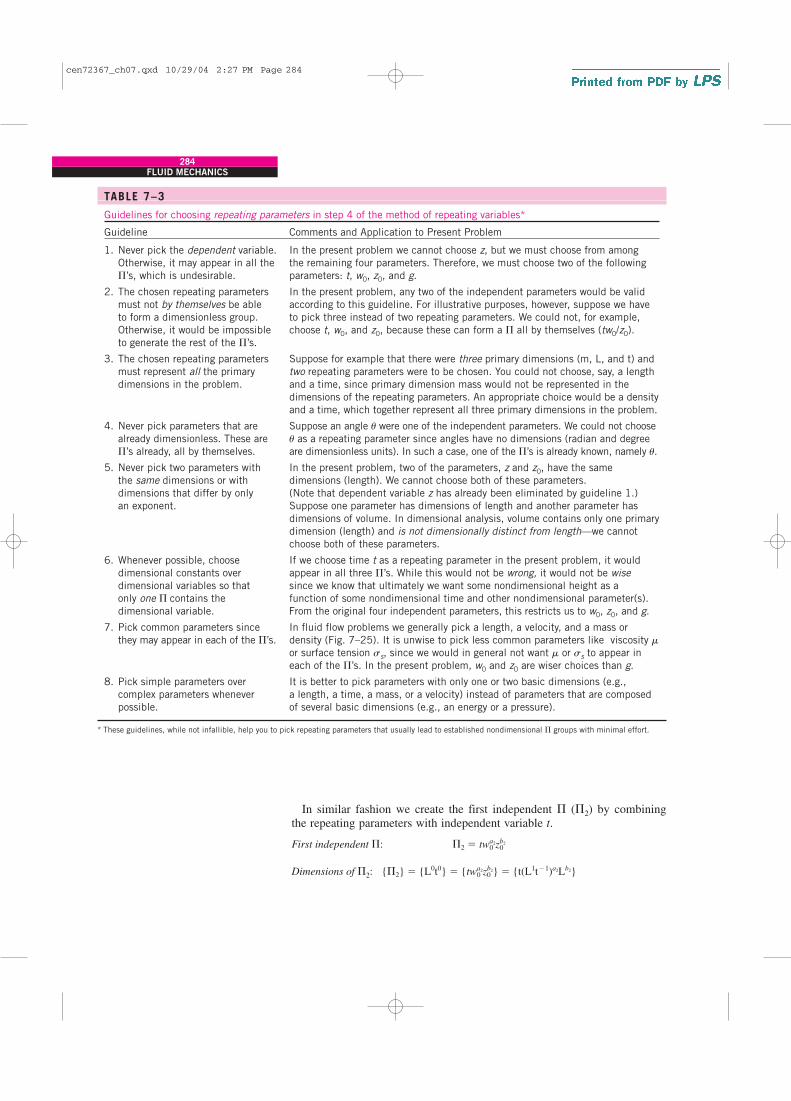
elevation z of the ball must be a function of time t, initial vertical speed w0,
initial elevation z0, and gravitational constant g (Fig. 7–23). The beauty of
dimensional analysis is that the only other thing we need to know is the pri-
mary dimensions of each of these quantities. As we go through each step of
the method of repeating variables, we explain some of the subtleties of the
technique in more detail using the falling ball as an example.
Step 1There are five parameters (dimensional variables, nondimensional variables,
and dimensional constants) in this problem; n � 5. They are listed in func-
tional form, with the dependent variable listed as a function of the indepen-
dent variables and constants:
List of relevant parameters: z � f(t, w0, z0, g) n � 5
282FLUID MECHANICS
TABLE 7–2
Detailed description of the six steps that comprise the method of repeating
variables*
Step 1 List the parameters (dimensional variables, nondimensional variables,
and dimensional constants) and count them. Let n be the total
number of parameters in the problem, including the dependent
variable. Make sure that any listed independent parameter is indeed
independent of the others, i.e., it cannot be expressed in terms of
them. (E.g., don’t include radius r and area A � pr2, since r and A
are not independent.)
Step 2 List the primary dimensions for each of the n parameters.
Step 3 Guess the reduction j. As a first guess, set j equal to the number of
primary dimensions represented in the problem. The expected
number of �’s (k) is equal to n minus j, according to the Buckingham
Pi theorem,
The Buckingham Pi theorem: (7–14)
If at this step or during any subsequent step, the analysis does not
work out, verify that you have included enough parameters in step 1.
Otherwise, go back and reduce j by one and try again.
Step 4 Choose j repeating parameters that will be used to construct each �.
Since the repeating parameters have the potential to appear in each
�, be sure to choose them wisely (Table 7–3).
Step 5 Generate the �’s one at a time by grouping the j repeating parameters
with one of the remaining parameters, forcing the product to be
dimensionless. In this way, construct all k �’s. By convention the first
�, designated as �1, is the dependent � (the one on the left side of
the list). Manipulate the �’s as necessary to achieve established
dimensionless groups (Table 7–5).
Step 6 Check that all the �’s are indeed dimensionless. Write the final
functional relationship in the form of Eq. 7–11.
* This is a step-by-step method for finding the dimensionless � groups when performing a dimensionalanalysis.
k � n � j
The Method of Repeating Variables
Step 1: List the parameters in the problem and count their total number n.
Step 2: List the primary dimensions of each of the n parameters.
Step 5: Construct the k II’s, and manipulate as necessary.
Step 6: Write the final functional relationship and check your algebra.
Step 4: Choose j repeating parameters.
Step 3: Set the reduction j as the number of primary dimensions. Calculate k, the expected number of II’s, k = n – j
FIGURE 7–22
A concise summary of the six steps
that comprise the method of repeating
variables.
w0 = initial vertical speed
z = 0 (datum plane)
z0 = initialelevation
g = gravitationalacceleration in thenegative z-direction
z = elevation of ball = f (t, w0, z0, g)
FIGURE 7–23
Setup for dimensional analysis of a
ball falling in a vacuum. Elevation z is
a function of time t, initial vertical
speed w0, initial elevation z0, and
gravitational constant g.
cen72367_ch07.qxd 10/29/04 2:27 PM Page 282
Step 2The primary dimensions of each parameter are listed here. We recommend
writing each dimension with exponents since this helps with later algebra.
Step 3As a first guess, j is set equal to 2, the number of primary dimensions repre-
sented in the problem (L and t).
Reduction:
If this value of j is correct, the number of �’s predicted by the Buckingham
Pi theorem is
Number of expected �’s:
Step 4We need to choose two repeating parameters since j � 2. Since this is often
the hardest (or at least the most mysterious) part of the method of repeating
variables, several guidelines about choosing repeating parameters are listed
in Table 7–3.
Following the guidelines of Table 7–3 on the next page, the wisest choice
of two repeating parameters is w0 and z0.
Repeating parameters:
Step 5Now we combine these repeating parameters into products with each of the
remaining parameters, one at a time, to create the �’s. The first � is always
the dependent � and is formed with the dependent variable z.
Dependent �: (7–15)
where a1 and b1 are constant exponents that need to be determined. We
apply the primary dimensions of step 2 into Eq. 7–15 and force the � to be
dimensionless by setting the exponent of each primary dimension to zero:
Dimensions of �1:
Since primary dimensions are by definition independent of each other, we
equate the exponents of each primary dimension independently to solve for
In similar fashion we create the first independent � (�2) by combining
the repeating parameters with independent variable t.
First independent �:
Dimensions of �2: {�2} � {L0t0} � {twa20 zb2
0 } � {t(L1t�1)a2Lb2}
�2 � twa20 zb2
0
284FLUID MECHANICS
TABLE 7–3
Guidelines for choosing repeating parameters in step 4 of the method of repeating variables*
Guideline Comments and Application to Present Problem
1. Never pick the dependent variable. In the present problem we cannot choose z, but we must choose from among
Otherwise, it may appear in all the the remaining four parameters. Therefore, we must choose two of the following
�’s, which is undesirable. parameters: t, w0, z0, and g.
2. The chosen repeating parameters In the present problem, any two of the independent parameters would be valid
must not by themselves be able according to this guideline. For illustrative purposes, however, suppose we have
to form a dimensionless group. to pick three instead of two repeating parameters. We could not, for example,
Otherwise, it would be impossible choose t, w0, and z0, because these can form a � all by themselves (tw0/z0).
to generate the rest of the �’s.
3. The chosen repeating parameters Suppose for example that there were three primary dimensions (m, L, and t) and
must represent all the primary two repeating parameters were to be chosen. You could not choose, say, a length
dimensions in the problem. and a time, since primary dimension mass would not be represented in the
dimensions of the repeating parameters. An appropriate choice would be a density
and a time, which together represent all three primary dimensions in the problem.
4. Never pick parameters that are Suppose an angle u were one of the independent parameters. We could not choose
already dimensionless. These are u as a repeating parameter since angles have no dimensions (radian and degree
�’s already, all by themselves. are dimensionless units). In such a case, one of the �’s is already known, namely u.
5. Never pick two parameters with In the present problem, two of the parameters, z and z0, have the same
the same dimensions or with dimensions (length). We cannot choose both of these parameters.
dimensions that differ by only (Note that dependent variable z has already been eliminated by guideline 1.)
an exponent. Suppose one parameter has dimensions of length and another parameter has
dimensions of volume. In dimensional analysis, volume contains only one primary
dimension (length) and is not dimensionally distinct from length—we cannot
choose both of these parameters.
6. Whenever possible, choose If we choose time t as a repeating parameter in the present problem, it would
dimensional constants over appear in all three �’s. While this would not be wrong, it would not be wise
dimensional variables so that since we know that ultimately we want some nondimensional height as a
only one � contains the function of some nondimensional time and other nondimensional parameter(s).
dimensional variable. From the original four independent parameters, this restricts us to w0, z0, and g.
7. Pick common parameters since In fluid flow problems we generally pick a length, a velocity, and a mass or
they may appear in each of the �’s. density (Fig. 7–25). It is unwise to pick less common parameters like viscosity m
or surface tension ss, since we would in general not want m or ss to appear in
each of the �’s. In the present problem, w0 and z0 are wiser choices than g.
8. Pick simple parameters over It is better to pick parameters with only one or two basic dimensions (e.g.,
complex parameters whenever a length, a time, a mass, or a velocity) instead of parameters that are composed
possible. of several basic dimensions (e.g., an energy or a pressure).
* These guidelines, while not infallible, help you to pick repeating parameters that usually lead to established nondimensional � groups with minimal effort.
cen72367_ch07.qxd 10/29/04 2:27 PM Page 284
Equating exponents,
Time:
Length:
�2 is thus
(7–17)
Finally we create the second independent � (�3) by combining the repeat-
ing parameters with g and forcing the � to be dimensionless (Fig. 7–26).
Second independent �:
Dimensions of �3:
Equating exponents,
Time:
Length:
�3 is thus
(7–18)
All three �’s have been found, but at this point it is prudent to examine
them to see if any manipulation is required. We see immediately that �1 and
�2 are the same as the nondimensionalized variables z* and t* defined by
Eq. 7–6—no manipulation is necessary for these. However, we recognize
that the third � must be raised to the power of to be of the same form
as an established dimensionless parameter, namely the Froude number of
Eq. 7–8:
Modified �3: (7–19)
Such manipulation is often necessary to put the �’s into proper estab-
lished form. The � of Eq. 7–18 is not wrong, and there is certainly no
mathematical advantage of Eq. 7–19 over Eq. 7–18. Instead, we like to
say that Eq. 7–19 is more “socially acceptable” than Eq. 7–18, since it is a
named, established nondimensional parameter that is commonly used in
the literature. In Table 7–4 are listed some guidelines for manipulation of
your nondimensional � groups into established nondimensional parameters.
Table 7–5 lists some established nondimensional parameters, most of
which are named after a notable scientist or engineer (see Fig. 7–27 and the
Historical Spotlight on p. 289). This list is by no means exhaustive. When-
ever possible, you should manipulate your �’s as necessary in order to con-
vert them into established nondimensional parameters.
Step 6We should double-check that the �’s are indeed dimensionless (Fig. 7–28).
You can verify this on your own for the present example. We are finally
ready to write the functional relationship between the nondimensional para-
meters. Combining Eqs. 7–16, 7–17, and 7–19 into the form of Eq. 7–11,
Relationship between �’s:
Or, in terms of the nondimensional variables z* and t* defined previously
by Eq. 7–6 and the definition of the Froude number,
Final result of dimensional analysis: (7–20)
It is useful to compare the result of dimensional analysis, Eq. 7–20, to the
exact analytical result, Eq. 7–10. The method of repeating variables prop-
erly predicts the functional relationship between dimensionless groups.
However,
The method of repeating variables cannot predict the exact mathematicalform of the equation.
This is a fundamental limitation of dimensional analysis and the method of
repeating variables. For some simple problems, however, the form of the
equation can be predicted to within an unknown constant, as is illustrated in
Example 7–7.
z* � f (t˛*, Fr)
�1 � f (�2, �3) → z
z0
� f ¢w0t
z0
, w0
2gz0
≤
286FLUID MECHANICS
TABLE 7–4
Guidelines for manipulation of the �’s resulting from the method of repeating variables.*
Guideline Comments and Application to Present Problem
1. We may impose a constant We can raise a � to any exponent n (changing it to �n) without changing the
(dimensionless) exponent on dimensionless stature of the �. For example, in the present problem, we
a � or perform a functional imposed an exponent of on �3. Similarly we can perform the functional
operation on a �. operation sin(�), exp(�), etc., without influencing the dimensions of the �.
2. We may multiply a � by a Sometimes dimensionless factors of , 2, 4, etc., are included in a � for
pure (dimensionless) constant. convenience. This is perfectly okay since such factors do not influence the
dimensions of the �.
3. We may form a product (or quotient) We could replace �3 by �3�1, �3/�2, etc. Sometimes such manipulation is
of any � with any other � in the necessary to convert our � into an established �. In many cases, the
problem to replace one of the �’s. established � would have been produced if we would have chosen different
repeating parameters.
4. We may use any of guidelines In general, we can replace any � with some new � such as A�3B sin(�1
C),
1 to 3 in combination. where A, B, and C are pure constants.
5. We may substitute a dimensional For example, the � may contain the square of a length or the cube of a
parameter in the � with other length, for which we may substitute a known area or volume, respectively, in
parameter(s) of the same dimensions. order to make the � agree with established conventions.
*These guidelines are useful in step 5 of the method of repeating variables and are listed to help you convert your nondimensional � groups into standard,established nondimensional parameters, many of which are listed in Table 7–5.
12
�12
Wow!
Aaron, you've made it! They named a nondimensionalparameter after you!
FIGURE 7–27
Established nondimensional
parameters are usually named after
a notable scientist or engineer.
cen72367_ch07.qxd 10/29/04 2:28 PM Page 286
287CHAPTER 7
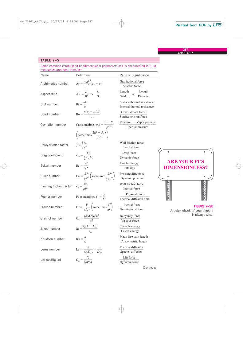
TABLE 7–5
Some common established nondimensional parameters or �’s encountered in fluid
mechanics and heat transfer*
Name Definition Ratio of Significance
Archimedes number
Aspect ratio
Biot number
Bond number
Cavitation number
Darcy friction factor
Drag coefficient
Eckert number
Euler number
Fanning friction factor
Fourier number
Froude number
Grashof number
Jakob number
Knudsen number
Lewis number
Lift coefficient
(Continued)
Lift force
Dynamic forceCL �
FL
12rV
2A
Thermal diffusion
Species diffusionLe �
k
rcpDAB
�a
DAB
Mean free path length
Characteristic lengthKn �
l
L
Sensible energy
Latent energyJa �
cp(T � Tsat)
hfg
Buoyancy force
Viscous forceGr �
gb 0�T 0L3r2
m2
Inertial force
Gravitational forceFr �
V
2gL asometimes
V˛
2
gL≤
Physical time
Thermal diffusion timeFo (sometimes t) �
at
L2
Wall friction force
Inertial forceCf �
2tw
rV 2
Pressure difference
Dynamic pressureEu �
�P
rV 2 asometimes
�P12rV
2≤
Kinetic energy
EnthalpyEc �
V 2
cPT
Drag force
Dynamic forceCD �
FD
12rV
2A
Wall friction force
Inertial forcef �
8tw
rV 2
asometimes 2(P � Pv )
rV˛˛
2 ≤
Pressure � Vapor pressure
Inertial pressureCa (sometimes sc) �
P � Pv
rV˛˛
2
Gravitational force
Surface tension forceBo �
g(rf � rv)L2
ss
Surface thermal resistance
Internal thermal resistanceBi �
hL
k
Length
Width or
Length
DiameterAR �
L
W or
L
D
Gravitational force
Viscous forceAr �
rsgL3
m2(rs � r)
ARE YOUR PI’S
DIMENSIONLESS?
FIGURE 7–28
A quick check of your algebra
is always wise.
cen72367_ch07.qxd 10/29/04 2:28 PM Page 287
288FLUID MECHANICS
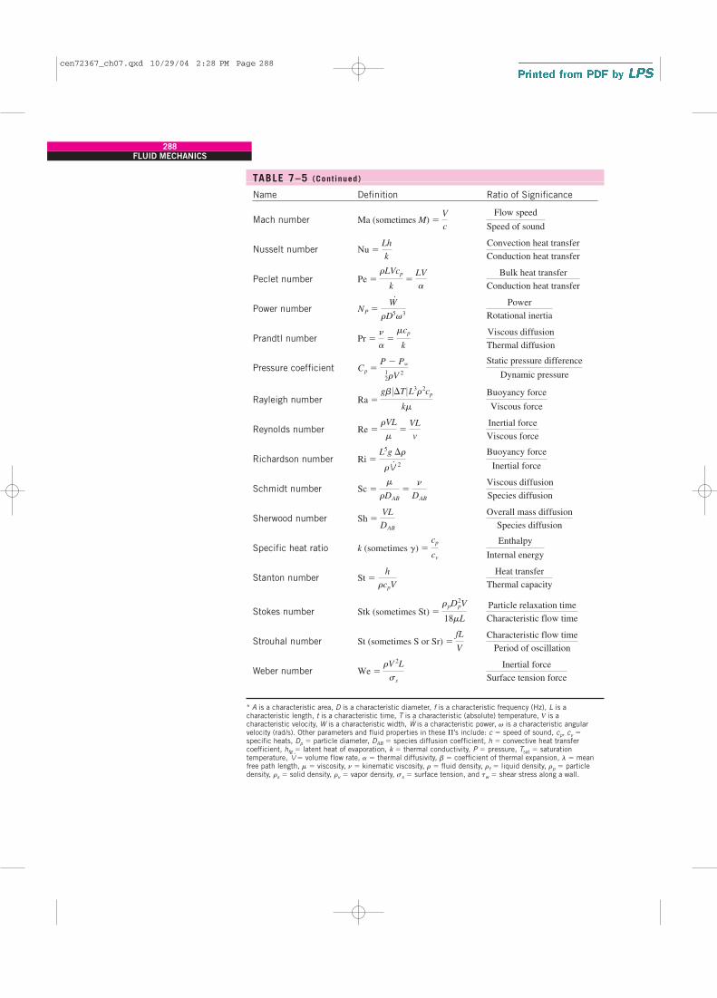
TABLE 7–5 (Cont inued)
Name Definition Ratio of Significance
Mach number
Nusselt number
Peclet number
Power number
Prandtl number
Pressure coefficient
Rayleigh number
Reynolds number
Richardson number
Schmidt number
Sherwood number
Specific heat ratio
Stanton number
Stokes number
Strouhal number
Weber number
* A is a characteristic area, D is a characteristic diameter, f is a characteristic frequency (Hz), L is acharacteristic length, t is a characteristic time, T is a characteristic (absolute) temperature, V is acharacteristic velocity, W is a characteristic width, W
.is a characteristic power, v is a characteristic angular
velocity (rad/s). Other parameters and fluid properties in these �’s include: c � speed of sound, cp, cv �specific heats, Dp � particle diameter, DAB � species diffusion coefficient, h � convective heat transfercoefficient, hfg � latent heat of evaporation, k � thermal conductivity, P � pressure, Tsat � saturationtemperature, � volume flow rate, a � thermal diffusivity, b � coefficient of thermal expansion, l � meanfree path length, m � viscosity, n � kinematic viscosity, r � fluid density, rf � liquid density, rp � particledensity, rs � solid density, rv � vapor density, ss � surface tension, and tw � shear stress along a wall.
V#
Inertial force
Surface tension forceWe �
rV 2L
ss
Characteristic flow time
Period of oscillationSt (sometimes S or Sr) �
fL
V
Particle relaxation time
Characteristic flow timeStk (sometimes St) �
rpD2pV
18mL
Heat transfer
Thermal capacitySt �
h
rcpV
Enthalpy
Internal energyk (sometimes g) �
cp
cv
Overall mass diffusion
Species diffusionSh �
VL
DAB
Viscous diffusion
Species diffusionSc �
m
rDAB
�n
DAB
Buoyancy force
Inertial forceRi �
L5g �r
rV#
2
Inertial force
Viscous forceRe �
rVL
m�
VL
v
Buoyancy force
Viscous forceRa �
gb 0�T 0L3r2cp
km
Static pressure difference
Dynamic pressureCp �
P � P�
12rV
2
Viscous diffusion
Thermal diffusionPr �
n
a�mcp
k
Power
Rotational inertiaNP �
W#
rD5v3
Bulk heat transfer
Conduction heat transferPe �
rLVcp
k�
LV
a
Convection heat transfer
Conduction heat transferNu �
Lh
k
Flow speed
Speed of soundMa (sometimes M) �
V
c
cen72367_ch07.qxd 10/29/04 2:28 PM Page 288
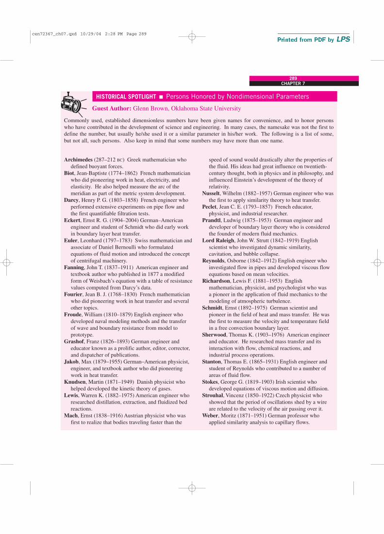
Guest Author: Glenn Brown, Oklahoma State University
Commonly used, established dimensionless numbers have been given names for convenience, and to honor persons
who have contributed in the development of science and engineering. In many cases, the namesake was not the first to
define the number, but usually he/she used it or a similar parameter in his/her work. The following is a list of some,
but not all, such persons. Also keep in mind that some numbers may have more than one name.
HISTORICAL SPOTLIGHT � Persons Honored by Nondimensional Parameters
speed of sound would drastically alter the properties of
the fluid. His ideas had great influence on twentieth-
century thought, both in physics and in philosophy, and
influenced Einstein’s development of the theory of
relativity.
Nusselt, Wilhelm (1882–1957) German engineer who was
the first to apply similarity theory to heat transfer.
Peclet, Jean C. E. (1793–1857) French educator,
physicist, and industrial researcher.
Prandtl, Ludwig (1875–1953) German engineer and
developer of boundary layer theory who is considered
the founder of modern fluid mechanics.
Lord Raleigh, John W. Strutt (1842–1919) English
scientist who investigated dynamic similarity,
cavitation, and bubble collapse.
Reynolds, Osborne (1842–1912) English engineer who
investigated flow in pipes and developed viscous flow
equations based on mean velocities.
Richardson, Lewis F. (1881–1953) English
mathematician, physicist, and psychologist who was
a pioneer in the application of fluid mechanics to the
modeling of atmospheric turbulence.
Schmidt, Ernst (1892–1975) German scientist and
pioneer in the field of heat and mass transfer. He was
the first to measure the velocity and temperature field
in a free convection boundary layer.
Sherwood, Thomas K. (1903–1976) American engineer
and educator. He researched mass transfer and its
interaction with flow, chemical reactions, and
industrial process operations.
Stanton, Thomas E. (1865–1931) English engineer and
student of Reynolds who contributed to a number of
areas of fluid flow.
Stokes, George G. (1819–1903) Irish scientist who
developed equations of viscous motion and diffusion.
Strouhal, Vincenz (1850–1922) Czech physicist who
showed that the period of oscillations shed by a wire
are related to the velocity of the air passing over it.
Weber, Moritz (1871–1951) German professor who
applied similarity analysis to capillary flows.
Archimedes (287–212 BC) Greek mathematician who
defined buoyant forces.
Biot, Jean-Baptiste (1774–1862) French mathematician
who did pioneering work in heat, electricity, and
elasticity. He also helped measure the arc of the
meridian as part of the metric system development.
Darcy, Henry P. G. (1803–1858) French engineer who
performed extensive experiments on pipe flow and
the first quantifiable filtration tests.
Eckert, Ernst R. G. (1904–2004) German–American
engineer and student of Schmidt who did early work
in boundary layer heat transfer.
Euler, Leonhard (1797–1783) Swiss mathematician and
associate of Daniel Bernoulli who formulated
equations of fluid motion and introduced the concept
of centrifugal machinery.
Fanning, John T. (1837–1911) American engineer and
textbook author who published in 1877 a modified
form of Weisbach’s equation with a table of resistance
values computed from Darcy’s data.
Fourier, Jean B. J. (1768–1830) French mathematician
who did pioneering work in heat transfer and several
other topics.
Froude, William (1810–1879) English engineer who
developed naval modeling methods and the transfer
of wave and boundary resistance from model to
prototype.
Grashof, Franz (1826–1893) German engineer and
educator known as a prolific author, editor, corrector,
and dispatcher of publications.
Jakob, Max (1879–1955) German–American physicist,
engineer, and textbook author who did pioneering
work in heat transfer.
Knudsen, Martin (1871–1949) Danish physicist who
helped developed the kinetic theory of gases.
Lewis, Warren K. (1882–1975) American engineer who
researched distillation, extraction, and fluidized bed
reactions.
Mach, Ernst (1838–1916) Austrian physicist who was
first to realize that bodies traveling faster than the
289CHAPTER 7
cen72367_ch07.qxd 10/29/04 2:28 PM Page 289
290FLUID MECHANICS
EXAMPLE 7–7 Pressure in a Soap Bubble
Some children are playing with soap bubbles, and you become curious as to
the relationship between soap bubble radius and the pressure inside the
soap bubble (Fig. 7–29). You reason that the pressure inside the soap bub-
ble must be greater than atmospheric pressure, and that the shell of the
soap bubble is under tension, much like the skin of a balloon. You also know
that the property surface tension must be important in this problem. Not
knowing any other physics, you decide to approach the problem using
dimensional analysis. Establish a relationship between pressure difference
�P � Pinside � Poutside, soap bubble radius R, and the surface tension ss of
the soap film.
SOLUTION The pressure difference between the inside of a soap bubble
and the outside air is to be analyzed by the method of repeating variables.
Assumptions 1 The soap bubble is neutrally buoyant in the air, and gravity is
not relevant. 2 No other variables or constants are important in this problem.
Analysis The step-by-step method of repeating variables is employed.
Step 1 There are three variables and constants in this problem; n � 3.
They are listed in functional form, with the dependent variable listed as a
function of the independent variables and constants:
List of relevant parameters:
Step 2 The primary dimensions of each parameter are listed. The
dimensions of surface tension are obtained from Example 7–1, and those
of pressure from Example 7–2.
Step 3 As a first guess, j is set equal to 3, the number of primary
dimensions represented in the problem (m, L, and t).
Reduction (first guess): j � 3
If this value of j is correct, the expected number of �’s is k � n � j � 3 �
3 � 0. But how can we have zero �’s? Something is obviously not right
(Fig. 7–30). At times like this, we need to first go back and make sure that
we are not neglecting some important variable or constant in the problem.
Since we are confident that the pressure difference should depend only on
soap bubble radius and surface tension, we reduce the value of j by one,
Reduction (second guess): j � 2
If this value of j is correct, k � n � j � 3 � 2 � 1. Thus we expect one �,
which is more physically realistic than zero �’s.
Step 4 We need to choose two repeating parameters since j � 2.
Following the guidelines of Table 7–3, our only choices are R and ss, since
�P is the dependent variable.
Step 5 We combine these repeating parameters into a product with the
dependent variable �P to create the dependent �,
Dependent �: (1)�1 � �PRa1sb1s
�P R ss
{m1L�1t�2} {L1} {m1t�2}
�P � f (R, ss) n � 3
Soap film
Pinside
Poutside
ss
ss
R
FIGURE 7–29
The pressure inside a soap bubble is
greater than that surrounding the soap
bubble due to surface tension in the
soap film.
What happens if
k 0?
Do the following:
Check your list of parameters.
Check your algebra.
If all else fails, reduce by one.
FIGURE 7–30
If the method of repeating variables
indicates zero �’s, we have either
made an error, or we need to
reduce j by one and start over.
cen72367_ch07.qxd 10/29/04 2:28 PM Page 290
We apply the primary dimensions of step 2 into Eq. 1 and force the � to be
dimensionless.
Dimensions of �1:
We equate the exponents of each primary dimension to solve for a1 and b1:
Time:
Mass:
Length:
Fortunately, the first two results agree with each other, and Eq. 1 thus
becomes
(2)
From Table 7–5, the established nondimensional parameter most similar to
Eq. 2 is the Weber number, defined as a pressure (rV2) times a length
divided by surface tension. There is no need to further manipulate this �.
Step 6 We write the final functional relationship. In the case at hand,
there is only one �, which is a function of nothing. This is possible only if
the � is constant. Putting Eq. 2 into the functional form of Eq. 7–11,
Relationship between �’s:
(3)
Discussion This is an example of how we can sometimes predict trends with
dimensional analysis, even without knowing much of the physics of the prob-
lem. For example, we know from our result that if the radius of the soap
bubble doubles, the pressure difference decreases by a factor of 2. Similarly,
if the value of surface tension doubles, �P increases by a factor of 2. Dimen-
sional analysis cannot predict the value of the constant in Eq. 3; further
analysis (or one experiment) reveals that the constant is equal to 4 (Chap. 2).
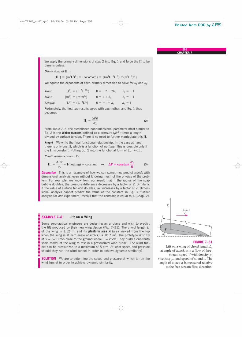
EXAMPLE 7–8 Lift on a Wing
Some aeronautical engineers are designing an airplane and wish to predict
the lift produced by their new wing design (Fig. 7–31). The chord length Lc
of the wing is 1.12 m, and its planform area A (area viewed from the top
when the wing is at zero angle of attack) is 10.7 m2. The prototype is to fly
at V � 52.0 m/s close to the ground where T � 25°C. They build a one-tenth
scale model of the wing to test in a pressurized wind tunnel. The wind tun-
nel can be pressurized to a maximum of 5 atm. At what speed and pressure
should they run the wind tunnel in order to achieve dynamic similarity?
SOLUTION We are to determine the speed and pressure at which to run the
wind tunnel in order to achieve dynamic similarity.
�1 ��PR
ss
� f (nothing) � constant → �P � constant Ss
R
�1 ��PR
ss
{L0} � {L�1La1} 0 � �1 � a1 a1 � 1
{m0} � {m1mb1} 0 � 1 � b1 b1 � �1
{t0} � {t�2t�2b1} 0 � �2 � 2b1 b1 � �1
{�1} � {m0L0t0} � {�PR˛
a1sb1s } � {(m1L�1t�2)La1(m1t�2)b1}
291CHAPTER 7
Lc
FL
V
r, m, c
a
FIGURE 7–31
Lift on a wing of chord length Lc
at angle of attack a in a flow of free-
stream speed V with density r,
viscosity m, and speed of sound c. The
angle of attack a is measured relative
to the free-stream flow direction.
cen72367_ch07.qxd 10/29/04 2:28 PM Page 291
Assumptions 1 The prototype wing flies through the air at standard atmos-
pheric pressure. 2 The model is geometrically similar to the prototype.
Analysis First, the step-by-step method of repeating variables is employed
to obtain the nondimensional parameters. Then, the dependent �’s are
matched between prototype and model.
Step 1 There are seven parameters (variables and constants) in this
problem; n � 7. They are listed in functional form, with the dependent
variable listed as a function of the independent parameters:
List of relevant parameters:
where FL is the lift force on the wing, V is the fluid speed, Lc is the chord
length, r is the fluid density, m is the fluid viscosity, c is the speed of
sound in the fluid, and a is the angle of attack of the wing.
Step 2 The primary dimensions of each parameter are listed; angle a is
dimensionless:
Step 3 As a first guess, j is set equal to 3, the number of primary
dimensions represented in the problem (m, L, and t).
Reduction: j � 3
If this value of j is correct, the expected number of �’s is k � n � j � 7 � 3
� 4.
Step 4 We need to choose three repeating parameters since j � 3. Following
the guidelines listed in Table 7–3, we cannot pick the dependent variable FL.
Nor can we pick a since it is already dimensionless. We cannot choose both
V and c since their dimensions are identical. It would not be desirable to
have m appear in all the �’s. The best choice of repeating parameters is
thus either V, Lc, and r or c, Lc, and r. Of these, the former is the better
choice since the speed of sound appears in only one of the established
nondimensional parameters of Table 7–5, whereas the velocity scale is
more “common” and appears in several of the parameters (Fig. 7–32).
Repeating parameters:
Step 5 The dependent � is generated:
The exponents are calculated by forcing the � to be dimensionless
(algebra not shown). We get a1 � �2, b1 � �2, and c1 � �1. The
dependent � is thus
From Table 7–5, the established nondimensional parameter most similar to
our �1 is the lift coefficient, defined in terms of planform area A rather than
the square of chord length, and with a factor of in the denominator. Thus,
we may manipulate this � according to the guidelines listed in Table 7–4