Discontinuous and Mixed Finite Elements for Two-Phase Incompressible Flow Guy Chavent, SPE, CEREMADE and INRIA; Gary Cohen, SPE, and .. erome "affre, SPE, INRIA; Robert Eymarcl, * Elf Aquitaine; and Dominique R. Guerillot, SPE, and Luce Weill, Inst. Frant,fais du Petrole

BeE 1601 8

Summary. The simulation of multiphase flow presents several difficulties, including (1) the occurrence of sharp moving fronts when convection is dominating, (2) the need for a good approximation of velocities to calculate the convective terms of the equation, and (3) flow singularities around wells. To handle the first difficulty, we propose a Godunov-type higher..order scheme based on a piecewise linear approximation of the saturation associated with a multidimensional slope limiter. With respect to the second, the pressure equa­tion is approximated by means of a mixed-hybrid formulation equivalent to the classic mixed formulation but yielding a positive-definite linear system. To solve the third difficulty, we introduce macroelements around wells. Numerical experiments illustrate the capabilities of the method.

Introduction In a previous paper, I we proposed a finite-element method (FEM) for 2D diphasic simulations. In addition to the global pressure for­mulation, 1.2 the basic tools for this method were a higher-order Godunov-type3 discontinuous FEM to approximate the saturation equation with little numerical diffusion and a mixed finite-element approximation of the pressure equation to reduce grid-orientation effects through better coupling of the pressure and saturation equa­tions. In this paper, we present new developments added to this method concerning the approximation of the saturation equation, the resolution of the pressure equation, and the representation of wells.

The discontinuous FEM consists of a discontinuous, piecewise, linear or bilinear approximation of the saturation that allows us to design a higher-order scheme. Inside each cell, the water­conservation equation is multiplied by test functions and integrat­ed by parts. Numerical fluxes approximating water flow rates on the edges are calculated at Gauss integration points on the edges by use of Godunov equations solving a ID Riemann problem and involving the two traces of the saturation at the Gauss points. Ex­tending ideas developed by Van Leer,4 we added a multidimen­sional slope limiter that greatly enhances the scheme's stability and that prevents overshoots and oscillations2 to the discontinuous FEM (see Ref. 5 for a similar approach).

For the pressure equation, the usual mixed finite-element formulation2•6•7 yields a linear system that is difficult to solve be­cause it is not positive-definite. To overcome this drawback, we use the equivalent mixed-hybrid formulation. 2•8 In addition to the pressure inside the cells and the total flow rates across the edges, this formulation introduces as new unknowns the pressure values on the edges. The original degrees of freedom can be eliminated to obtain a linear system in the new unknowns that is symmetric, positive-definite, and easy to solve.

Finally, well models called macroelements9 are presented. A un­ion of cells around a well is divided into several sectors inside which the flow is assumed to be radial and is calculated through a simpli­fied to simulator in radial coordinates, For each well, a finite num­ber of I D radial problems (the macroelement) links the finite-element variables to the well variables, allowing for direct calculation of the bottomhole pressure (BHP), for example, and for precise calculation of water breakthrough. With such a method, one can simulate in particular nonradial flow around producing wells.

All these features are incorporated in the BIDIMIX simulator for two-phase incompressible flow developed jointly by INRIA, Inst. Francais du Petrole (lFP), and Elf Aquitaine. Performance of the

• Now at LaborBtoire Central des Pants et Chaussges.

Copyright 1990 Society 01 Petroleum Engineers

SPE Reservoir Engineering. November 1990

simulator is demonstrated on four different numerical tests: a com­parison with a first-order finite-difference method on a simulation of a quarter of a five-spot pattern, an edgedrive coning problem, an imbibition problem, and a field-scale problem.

Saturation Equation Ref. 1 describes the saturation equation in detail. The water­conservation law is

t/J(x)(iJSwr/iJt)+V· "w=O, ........................... (1)

where the water volumetric flow vector, "w, can be written as

"w=r+bo(Swr)u,+bl(Swr)qj +b2(Swr)~ . ......... ,. (2)

Here, the usual terms have been rearranged in such a way that each physical effect is clearly identified: r= -y,(x)P cmax(x)V[a(Swr)) is the capillary diffusion term; bO(Swr) U, is the standard transport term, with the fractional flow, bo, and the total water/oil flow vec­tor, u,; b l (Swr)ifi describes the differential action of gravity on the two fluids, with qj proportional to VD(x); and b2(Swr)~ describes the differential action of capillary pressure heterogeneity on the two fluids with iii proportional to VP cmax(x).

The last three terms will be approximated in the same way; there­fore, it is convenient to introduce the transport term

2

!<x,Swr)=bo(Swr)u,+ E bj(Swr)'ifj· ................ (3) j=i

Typical boundary conditions for these equations are

"w ·P=O ........................................ (4)

on the outer boundary, r t, of the field,

Swr=l .......................................... (5)

(given water injection rate) on the boundary, r e' of an injection well; and

r·p=O ......................................... (6)

(capillary effects neglected) on the boundary, r s' of a production well.

The initial condition is

Swr=SwrO at t=O . ................................. (7)

Discontinuous Finite-Element Approximation of Saturation. The reduced saturation, Swr' is approximated by SwraeM1, which is linear on every Triangle (bilinear on every Parallelogram) K of the finite-element mesh covering the field domain (see Fig. 1). By use of forward differencing in time, the saturation is obtained at each timestep through a two-step calculation. The first step is a finite­element calculation, and the second step limits the slope of the satu­ration calculated in the first step.

567

,-x

fig. 1:-Degrees of freedom for approximation spaces ",0, "t, i, end Y.-

First, an intermediate saturation S::tt 1 eMl is calculated with the discontinuous FEM described in Ref. 1. Eq. 1 is written on every Element K of Mesh Td,multiplied by test functions v lying in MI, and the transport term is integrated by parts. In this man­ner, we obtain the approximation equatioo:

s*n+l -sn J J wnI wnI v+J (Vr;,n)v- J k(x,snwra)· Vv+ E F1v=0 K III K K ACaK A

for all veM1 , KeTd • . •.. .••....•.. •.•• .••••.•.•••.•. (8)

Here, F1 represents some approximation of the normal component of k(x.S~) across A, which is described below. When capillary effects are neglected, I FA is the approximate water flow rate across A. A

Taking v constant over K in Eq. 8 gives equations for the mean values of S*..:r,+ l over the elements that are very similar to the equa­tions obtained by the finite-volume discretization method and that express water conservation in each cell. The other choices for v will determine the shape of S-::a+ lover K. Eq. 8 results in a ser­ies of simple 3 x 3 or 4 x 4 linear systems, depending 00 whether K is a triangle or a parallelogram; thus, the determination of S~+ 1

can be considered explicit. The approximate diffusion term, r;,n, is taIren to lie in the

Raviart-Thomas finite dimensional space X of lowest order. The space X is described in Fig. 1. Functions of X are uoiquely de­fined by their fluxes across the edges of the discretized domain. The calculation of r;,n is achieved by solving the linear system

(.,-1 rnVs J p a = J a(~rcz)Vs-J a(l)s' r-J a(S~a)s' r o cmax 0 re r,ur. for all seX such that s· .. =O 00 rturs , ........... . .. . (9)

r;,1I'rIA+F1=Ofor all Aert ... .... .......... .... (10)

and r;.1I·r=O 00 rs ....... ....... .... .............. (11)

where S~ra is a piecewise constant approximation of the trace of Swr on rturs.

The approximate transport term, k. is defined by approximating in X the vector fields u,. q.. and 7ii and by setting for any xeD and for any saturation value S

2

k(x.S)=bo(S)u,a+ E bj(S)iija(x) . ................ (12) j=1

568

The approximate total flow vector. u,ad. is calculated when the press~reequation is solved (see below). and vectors iliad. 7haeX are given by preliminary calculations.

The boundary term, FA. is calculated at the Gauss integration points of Edge A by solving approximately 10 generalized Rie­mann problems at these points for the function S-+ k(x.S) 'iA., FA is given by Godunov3 equations as a function of the two limit values S + and S - of the saturation S ~ra at x €.A.:

[

min k(x.k)· 'iA. if S- sS+ , ke[S- .S+]

FA (x) = max k(x.k)· 'iA. if S+ sS- ......... (13) ke[S+ .S-] .

If the function S-+ k(x.S)· 'iA. is monotone, FA(x) is just the value of that function for the upstream limit value of the saturation.

This higher-order FEM, when used alone (i.e., when S':Ja1 = S*..:r,+l) has been shown 1,2 to give.very sharp fronts, but to suffer2

from a very restrictive stability condition (1lIId"l. s constant) and from an antidiffusive behavior; i.e., the computed front lags be­hind its exact position. To correct these defects, we introduce a slope limiter.

Slope Limitation. The idea of limiting slopes in higher-order schemes for hyperbolic equations comes from Van Leer.4 The slope limiter introduced by Cockburn and Jaffre for the FEM uses the same basic idea. An additional parameter, 0, allows adjustment of the amount of diffusion introduced by the slope limiter. We describe the 20 version of this slope limiter for a general mesh with triangles and parallelograms. .

For a function v in Ml, denote by vK its restriction on Element K of Td and byvK its mean value over K, and define at every ver­tex M of the mesh

Sorln(M)=min {S;} ........... . ... .. ....... . .... (l4a) K3M

and Smax(M) = max {S;} . ...... . .. . . .. .. ........... (l4b) K3M

Then, for a given Oe(O,I) and a given Element K of the mesh, we define a set AK of admissible functions vK that are restrictions to K of functions veM l such that (I)

VK=S; ............... . . . . . .... . .. . . .... ....... (15a)

(maintains conservativity) and (2) at each vertex M of K, v(M) satisfies

(1-0)S;+OSmin(M)sv(M)S(I-0)S;+OSmax(M) .... (l5b)

(limits the slope). Finally, S;+I is selected in AK such that it is the projection of S; n+ lover A K; precisely, S;+ 1 minimizes over A K the distance friilction

Ilv-S;II+l112=~ E [v(M)-S;(M)]2 .. . . ... (16)

M=vertex of K. Mvertex of K

Ref. 5 gives another war. of selecting SK+ 1 in AK . Of course,' for 0 =0, one gets S" + 1 = S* =constant, so the method reduces to a fmite-volume meth& witIfpiecewise constant saturations that is known to be stable but very diffusive. For 0=1, the method has been found2 to restore a satisfying stability condition,

vmax(llI/d)s~, ................................. (17)

but is not diffusive enough, positioning numerical fronts behind their theoretical position. Numerical experiments for Buckley-Leverett disp1acements2 have shown that 0 values ranging from 0.3 to 0.5 gave a good compromise between diffusion and precision; the value 0=0.5 is u~ in the numerical results presented below. The sta­bility condition in the general case seems to be2

vmax(llI/d)s[l/(l +0)] . ........... . ............... (18)

From a practical viewpoint, the calculation of Sa-hi necessitates the resolution, on each Element K, of a 30 or 40 optimization

SPE Reservoir Engineering. November 1990

K -- -....... ~ E1 E: ~,

"'x . x x

K [' 1 ,] x x x

" x x

x x x

The matrix DrV· x x x

" x x

X It X

X X X

" X " . The matrix AQ*

K K' ...-.::-...~ ~

D - E ;) r 0 -. F ~

. 0 -1 -1 DeKnK' 0

I . .

0 I a I I r

E -1 Eereur t r ... 0 I qd

I ecges

1 The matrix a

Fer s f

~------I--- -_. I , Pd I I .

The matrix I s FTI

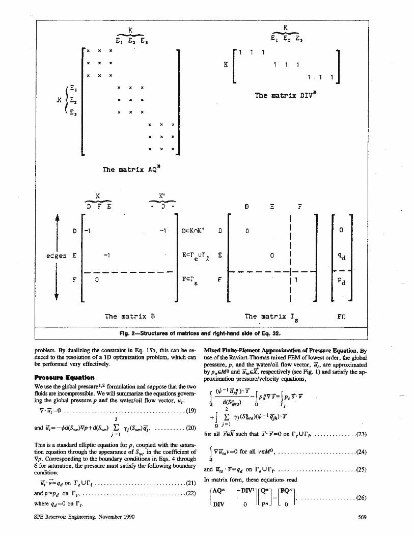
Fig. 2-Structures of matrices and right-hand side of Eq. 32.

problem. By dualizing the constraint in Eq. 15b, this can be re­duced to the resolution of a ID optimization problem, which can be performed very effectively.

Pre.sure Equation We use the global pressure 1,2 formulation and suppose that the two fluids are incompressible. We will summarize the equations govern­ing the global pressure P and the water/oil flow vector, "t:

V'u,=O ........................................ (19) 2

and u,= -tfd(Swr)Vp+d(Swr) E 'Yj(Swr)(jj. . ......... (20) j=1

This is a standard elliptic equation for p, coupled with the satura­tion equation through the appearance of Swr in the coefficient of Vp. Corresponding to the boundary conditions in Eqs. 4 through 6 for saturation, the pressure must satisfy the following boundary condition:

u,' P=qd on reUr, .............................. (21)

and P=Pd on rs , ..•.......•...•.................•. (22)

where qd=O on r (.

SPE Reservoir Engineering, November 1990

Mixed Finite-Element Approximation of Pressure Equation. By use of the Raviart-Thomas mixed FEM oflowest order, the global pressure, P, and the water/oil flow vector, u" are approximated by PaeMO and "taeX. respectively (see Fig. 1) and satisfy the ap­proximation pressure/velocity equations,

J (tf-I un)""s J J __ ..:.:ta ___ p;Vs= Pe s' v

o d(S~a) 0 r 2 s

+ J E 'Yj(S':vra)(tf- 1 (jjh)' S o j=i

for all sex such that s· v=O on r"ur" .............. (23)

J Vu,av=O for all veMD, .......................... (24) o

and U,a'V=qd on r"ur, ........................... (25)

In matrix form, these equations read

.................. (26)

569

Fig. 3-We" and ftnlt .. lement mesh.

where QII and PII are given by values of the degrees of freedom of U,aEX and Pl1 eM° , i.e., the fluxes qJ of Ii,: through any Edge A and the constant value PI of the pressure P 11 over any Element K. Thus, Eq. 26 is a linear system of dimension na +nt +nq, where na' nt, and nq are the numbers of edges, triangles, and quadrilater­als in the mesh, respectively.

The matrix of the linear system in Eq. 26 is not positive-<iefinite, however, so much work has been done to solve it efficiently. 16-14

In Ref. 1, the incompressibility of the flow was used to calculate Uta in the subspace of X of divergence-free functions. This method is very inexpensive but cannot be extended efficiently to compres­sible flow. The augmented Lagrangian technique used in Ref. 9 is more general, but its drawback is the necessity to adjust a pa­rameter to obtain fast convergence. To overcome these difficul­ties, we turned to the mixed-hybrid formulation2•8 of the pressure equation, which gives a general, convenient, and efficient way to calculate P a and u,a'

Mixed-Hybrid Finite-Elemeat Solution of the Pressure Equa­tion. First, we replace the v.ector field Ii"to with continuous flux­es across the edges by a vector field liia" with DO such continuity requirement (see Fig. 1). Thus, the degrees of freedom of liia"will be qK,A for KeTd and A CaK(3nt +4nq degrees of freedom). The continuity of the fluxes of Ii':o across edges will be enforced ex­plicitly. Then, we introduce new unknowns,.p A' representing ap­proximate pressure values_ on Edges AeAd. The P A are the Lagrangian multipliers of the continuity constraints imposed on the fluxes of uia". The mixed-hybrid finite-element approximation equations are

J(1/I-IU

:')'S_ E [JPaVS- E PAJS'PK]= o d(S~a) KeTd K ACaK A

2

E J 'Yj(S~ra)(1/I-1 qjh)' S for all sEX* • ......... .. (27) j~1 0 .

J Vu:a"v=O for all veMO, .... .. .... .... ........ .. (28) o qK,A +qK'.A =0, KnK'=A, for all AeAd, A(tr"Ur t , .. (29)

qK,A=qd for all ACr"Ur(, ....................... (30)

and PA =Pd for all A crs ' .. . .. .... . .... . .... . . . . . . .. (31)

In matrix form, these equations can be written as a linear system in the unknowns Q*(qK.A' KeTd, ACoK), P=(PK, KeTd), and n=(PA' AeAd)

570

[

AQ*

DIV*

B

Fig. 4-Macroelement.

DIVt.

B;t][Q:*] = [FQ~*. ]. ........ .. .. (32) o

o

Fig. 2 gives the structures of Matrices Aq-, DIV*, B, and Is and of Fn. It is clear from Eq. 29 that the function uta has con­tinuous fluxes across the mesh edges, so the solution (~, Pa) of Eqs. 27 through 31 coincides with the solution (u,a' Pa) of Eqs. 23 through 25. Therefore, we can replace the resolution of the linear system in Eq. 26 by that of the larger linear system (Eq. 32). But in Eq. 32, the matrix AQ* is 3 x3 or 4x4 block-diagonal (see Fig. 2), so we can eliminate the unknown Q*. In the resulting system in (P,II), the diagonal block corresponding to P is a diagonal matrix and also can be eliminated. Hence, we are left with a linear system in n only:

[ls+B·AQ*-I·tB_B ·AQ·-I·B'-B·(DIV*·AQ*-1

xDIV*t)-I·DIV*·AQ*-I·Bt)·n

=nI-B'AQ*-I<FQ*-DIV*')

x (DIV*' AQ* -I . DIV*') -I . DIV*' AQ* -I . FQ*). . . .. (33)

Despite its apparent complexity, Eq. 33 is a sparse, synunetric, positive-definite system, 2 with dimensions equal to the number of mesh edges. Thus Eq. 33 is very easy to solve-for example, by conjugate gradient with preconditioning. lOOn the pressures inside each element, P K are obtained by solving a diagonal system, and the fluxes, qk,A, by solving 3 x 3 or 4 x 4 systems on each element.

Approximation of W .... b, Radial GrIeI Refinement (liacro ... menta) To model the wells accurately, we used a grid-refinement technique that takes advantage of the essentially radial nature of the flow near the wens without imposing any symmetry of revolution on the sin­gularity (in opposition to nxrthods where the singularity, which is hand-calculated from a radially symmetric model, is subtracted from the solution). The method is described in detail in Ref. 9 and sum­marized as follows for an injection wen.

The actual boundary of the wen. r '" is replaced for the finite­element solver by a larger boundary, r eh' in such a way that (see Fag. 3) the mesh has not J>een refined in the vicinity of the wen; the well stands approximately in the center of the hole in the finite­element mesh; and the flow pattern is approximately radial in the domain covered by this hole.

SPE Reservoir Engineering, November 1990

--- ___ Bidimix, 8x8 grid .Jf

/) ,

......... 1st Order F. D.,24x24grid " , , , I ,/

_Exact Solution ' I ,.1

: / I

I I

( I

/\ I I I I I I

/ I i , I I

/ I I I I , : . ,

/ I I I

, I , . / I I

· I I . . • I I

/ : I I : I I

/ • I I · , I

/ : I I · , I

/ : I I

.' I · . I

/ ., , i

0/ i: I

~

FIg. 5-Saturatlon contours 0.1 and 0.9 at 0.7 PVI for a quarter of a five-spot linear displacement.

The flow between the well boundary, r e' and the finite-element boundary, r eh' is then modeled by a small number of 1 D radial models linking the well to each Gauss point of the edges of r eh

(see Fig. 4). We call a macroelement the collection of all these ID models. Within each macroelement, the flow can be calculated by any appropriate method. For simplicity, we used an implicit, first­order, finite-difference method and neglected gravity and capillary effects.

This method is very inexpensive in computation time and very flexible for the representation of actual wells because it allows direct determination of the BHP, taking into account the well radius and possible skin effects (by adjusting the porosity and permeability dis­tribution in each of the lD models).

Numerical Re.ults The method has been tested on four problems.

Problem 1. A quarter of a five-spot linear test problem for com­parison of results with an exact solution and a classic finite-difference simulator.

Problem 2. A coning model with highly adverse mobility ratio to test the sensitivity of the solution to mesh size and to demon­strate the interest of nonuniform grids.

Problem 3. A laboratory imbibition experiment to show the ability of the method to handle strong capillary effects.

Problem 4. A field-scale problem that exhibits the full potential of the method.

Problem 1. A quarter ofa 480x480x 100m five-spot pattern with 0.24 porosity, 140-md permeability, cross relative permeabilities,

TABLE 1-NUMBER OF TIMESTEPS AND VAX111780 CPU TIME FOR FIRST -ORDER FINITE-DIFFERENCE AND

BIDIMIX SIMULATIONS FOR PROBLEM 1

24x24 8x8 Finite-Difference BIDIMIX

Number of timesteps for 1 PVI

Overall computing time for 1 PVI. minutes:seconds

Computing time per timestep. seconds

Average volume injected per timestep per cell. fraction of cell PV

SPE Reservoir Engineering. November 1990

400 78

16 min 2:48

2.4 2.15

1.44 0.82

100r-----------------------~ I

a:: o ~

-- Exact Solution

____ Bidimix, 8x8 grid

_._ 1st Order F.D., 24x24 grid

.. l

/ ;:

/ .I

Fig. 6-WOR's for a linear displacement.

I I .

I

2.5

a mobility ratio of I, no capillary pressure, and a zero initial water saturation has been produced with a 10-MPa pressure drop between the injection and production wells. The results of simulations with the BIDIMIX code on a regular 8 x 8 grid and with the WFLOOD code of IFP on a regular 24 x 24 grid are compared with the exact analytical, solution. IS As shown in Fig. 5, the BIDIMIX front is much steeper than the fmite difference one, despite the much coarser grid used. For an exact water breakthrough of 0.707 PV injected (PVI), the 8 X 8 BIDIMIX simulation yields a 0.67 PVI computed value, compared with the 0.56 PVI value obtained by the 24x24 finite-difference simulation.

The WOR curves in Fig. 6 show that, after 1.5 PVI, the BIDI­MIX curve is much closer to the exact curve than is the finite­difference one. These gains in precision were not obtained at the price of high computation times, as Table 1 shows. '

In this linear test problem, BIDIMIX gave better results than ftrst­order [mite differences in roughly one-sixth the computation time. Credit has to be given to the higher-order scheme used for the satu­ration equation.

Problem 2. Numerical simulation of edgedrive coning problems with high adverse mobility ratios with finite-difference simulators are known to give answers that depend strongly on the mesh size. The behavior of the BIDIMIX code in that situation was tested on the edgedrive problem in Table 2 with the three different meshes in Fig. 7. Fig. 8 shows the results. Of course, the water produc­tion rate obtained by BIDIMIX depends on the mesh, which is not

TABLE 2-DATA FOR THE EDGEDRIVE CONING EXPERIMENT

Size. m Radius Thickness

PorOSity. % Permeability, md Viscosities, mPa' s

ILw ILo

Densities. g1cm 3

Pw Po

Initial aquifer thickness. m Injection boundary, m 3/d Production boundary. MPa

Sw krw o 0 0.2 0.8 1 1

kro 1 0.2 o

!.£. o

480 220

24 140

1 200

1 0.8 100 100 32

571

.. 064

~ ~ ~~ ~~ ~ ~~ I~~> '~~~

~ ~ ~ ~ ~~ ~~ ~~ ~ ~~.

,

0 99T35

~~ ~ ~ ~ ~ f~~ ~ ~ . ,,;.

.~~ ~ ~ ~~ ::~~ ~ ~' ~.\~ ~\, .~., :\:','

0256 ~0:: ' , ~ I'\." ~ '\., ,~ ' ;.\ "., ,~ ~'\ ..L

I~ F:\~ ',' '\ ~'\. ~" :-...~ ' :', !:\'~ :-.:, >~\. ~,

~ . ,,\ ~ ,,\ ' , " .. ' " '\" ~" ::-\:, ',::-.; 0-.'\ '\: , .. ::-; ~~'\ ~ t'.'\ ~ " ",' f~ 0.~ 10..'. ~'\ ~ ~

....-

Fig. 7-Th .... meshes UHd for BlDIMIX simulations of the edgedrtve coning problem.

surprising because the problem is unstable (mobility ratio of 2(0). The shapes of the curves are quite alike, however, and the change in breakthrough time is on the order of only 10%. On the coarse mesh, Q64, the breakthrough is delayed because numerical diffu­sion prevents the development of the water tongue toward the pro­duction boundary.

The results obtained on the two refined meshes, Q99T3S and Q2S6, are very similar. This similarity shows the interest of local refmement allowed by the use of triangular elements. Q99T35 con­tains half as many elements as Q256. Table 3 shows the gain in computing time.

Problem 3. In this experiment, a paraUelepipedic sandstone slab, which was previously saturated with oil, was immersed vertically in brine. During the imbibition process, the two ends of the slab were horizontal and the four lateral sides were vertical. Two of the lateral sides were impervious (see Table 4 and Fig. 9 for more data) . Similar experiments were performed in IFP laboratories. From a numerical viewpoint, this simulation illustrates the behavior of the model when only gravity and capillary forces are present.

The simulation was performed with a 50 X 5 mesh of 250 square elements; the oil recovery after 10 hours was about 44.6% of the initial volume of oil-i.e. , 95% of the recoverable oil. As Fig. 10 shows, initial oil flow rates through vertical faces were about 10 times greater than the flow through the lower and upper horizontal face, which corresponds to the ratio of the areas of the faces . Of course, recovery through the lower face is less than that through the upper face because of the gravity forces. Fig. 11 shows the re­duced saturation after 1 minute of imbibition, which illustrates brine penetration through the four slab faces.

572

TABLE 3-CPU TIME FOR THE EDGEDRIVE CONING PROBLEM (CRAY 1)

Mesh

Q64 Q99T35 Q256

Computing time per timestep. seconds 0.13 0.23 0.53

Number of timesteps for 1,ooQ-day simulation 300 1,100 1,100

100~ ______________________ ~ w

~

064 ·············099T35 -'-'- Q256

E(DAYS) 1000

Fig. 8-Water production rates calculated by BlDlMIX for the edgedrtve coning problem.

Problem 4. An oil reservoir sitting on top of an aquifer was pr0-duced by waterdrive (see Table 5). The region saturated with oil is represented at initial time by the dashed area in Fig. 11. Two producing wells are located in the oil field. The simulation takes into account gravity effects but no capillary pressure effect. Fig. 12 also shows the discretization of the domain of simulation and points out the convenience of using triangles to follow the fronti­ers of the oil field and to refine locally. The two wens are modeled with macroelements covering one triangle. Because of the high m0-

bility ratio, water soon arrives at the producing wells in a flow without radial symmetry (see Fig. 13).

ConcIU8Ions 1. An FEM that associates discontinuous fmite elements for the

saturation equation, mixed-hybrid finite elements for the pressure equation, and macroelements has been shown to be feasible for two­phase incompressible flow models including gravity and capillary pressure effects and wells. .

2. The discontinuous FEM includes a bighec-order Godunov-type scheme and a slope limiter. This yields a large reduction in numer­ical diffusion and front smearing coqmed with first-order schemes.

3. The mixed"hybrid formulation of the pressure equation leads to a symmetric, positive-definite, linear system and provides an ef­ficient alternative to the mixed formulation.

4. Macroelements are flexible tools to model flow in the vicini­ty of wells. In paiticular, they can simulate flows that are not radi­ally symmetric around wens.

TABLE 4-DATA FOR THE LABORATORY IMBIBITION EXPERIMENT

Dimension of the slab Length, cm Section (square), cm2

Porosity, % Permeability, md Fluid 1 Fluid 2 Vicosities, mPa· s

P-w P-D

Densities, glcm 3

PIIII Po

48.9 24

10.9 306

brine (water + 30 giL NaCI) oil (Soltrol™ 130)

1.048 1.52

1.019 0.758

Relative permeability and capillary pressure curves

Boundary conditions on pervious sides HydrauliC potential Initial condition

Fig. 9 5..,-1

constant 5 ... 0 .. 0

SPE Reservoir Engineering, November 1990

'~r---.---------------------------

~ '" • - 110 w • ~100

~ to

~ : ~

:~1-----~~;-----cw~----=;~;:::::~~----, WAlUI SATURATION 1"41

a

.~

.. ~

•. » 1 j .~

'"

• » ~ ~ ~

'IIIlTER SATURATlOHl"IU

b

Fig. 9-(.) Relative permeebilltJes and (b) caplltary pr1IUUrtI curv .. for tlHllmblbltJon .mut.lon.

,'0-0----------------------------,

:E 10'

.. ~

~ ~ 10"

~ all,.·

,,.. ,,-;,----------:l;;---------..,----'-------:' • •

TJM£ (HOURS)

fig. 10-Calculated 011 flow ratealn the Imbibition IImulatlon.

S. Irregular meshes including triangular elements are very con· vemenl for local refinements and for discretizing along frontiers and reservoir fractures.

SPE Reservoir Engineering, November 1990

z 0.70

G. 6S

O.BO ~

"" [g i2

0 .40 ~

x Fig. 1'-Perepectlve vI_ of reduced .. tunttlon In the slab after 1 minute of ImblblUon.

TABLE 5-DATA FOR TliE FIELD PROBLEM

Geometry, m Thickness, m Depth, m Porosity,% Permeability, md Densities, g/cm 3

p­p,

1300 x 1300

• from 590 (boundary) to 530 (near wells) 30

1,000

1 0.8

Viscosities, mPa·s

"-,,"0 •. Boundary condItIOns

0.5 40

Given pressure on the boundary (15.05 MPa) Two production wells (40 m3/d each)

Initial condition: water and 011 at equilibrium (Fig. 12)

~ lk ~ ~ 0.25 a 0.8 0 0.35 0.015 0.38 0.45 0.045 0.175 0.55 0.08 0.07 0.65 0.16 0.035 0.75 0.27 0

Nomenclatu,. a(S ..... ) = [(>. ... >.,,/(>. ... + >',,)](dP c/dS ..... ) (positive)

A = mesh edge Ad = set of all mesh edges

bo(S ..... ) = >.,.)(}.. ... +>.,,) (increasing) b,(S ..... ) = [X ... >'"/(>' ... +>',,)](2(P ... -p,,)/(P ... +p,,») b2(S ..... ) = [>' ... >'"/(}.. ... +>'"liPc(S ..... )

d = largest diameter of mesh elements

d(S ..... ) = >' ... +>'" _ D(x) = depth 2 f(X,S ..... ) = bo(S ..... )u,+E b.(S )q. j_' J ..... J

573

fig. 12-The 379-element mesh for the reservoir simulation.

_ 2

f a(X,Swr) = bO(Swr)iIIa + 1: b · (S )q. j =1 Ja wr Ja

FA. = Godunov numerical flux of T across A g = gravity coefficient

krj = relative permeability of water (j = w) or oil (j =0) K = mesh element

MO = constant vlvlK for all KeTd MI = linear vlvlK if K is a triangle (bilinear if K is a

parallelogram) for all KeTd na = number of edges of Ad ne = number of elements in mesh nq = number of parallelograms of Td n, = number of triangles ofTd P = global pressure 1.2

Pa = approximate global pressure (PaeMO) P A. = pressure on' Edge A PK = pressure in Element K (degree of freedom of Pa)

P cmax(x) = maximum capillary pressure at Point xl.2 Pc(Swr) = reduced capillary pressure function l •2 (increasing)

qA. = total flow rate across Edge A (degree of freedom of u,a)

574

q d = given total flow rate on r t ~a = approximation of ~ in X. j =0, 1, 2

qK,A. = total flow rate across Edge A coming out of K (degree of freedom of ilia)

qj = ~,y(x)(Pw +Po)gVD(x) iii = -,y(x)VP cmax(x) r: = -,yP cmax Va(Swr) = capillary diffusion flow vector

r;, = approximate capillary diffusion flow vector (~eX">

_ s = test function in X SK = mean value of Swro over K SK = restriction of Swra to K Sw = water saturation

Swc = water saturation at which capillary pressure vanishes

Swr = reduced water saturation, dimensionless Swra = approximate reduced water saturation (SwroeM 1)

Td = flnite-element mesh U, = total oil/water Darcy velocity (Eq. 20)

ilia = approximation of U, in X*

Contour. (.26, .35, .45,.55 . . 65,.74)

Fig. 13-Saturatlon contoura at 4,000 days.

u: = water Darcy velocity v = test function in MO or MI

Vmax = maximum velocity

X = [SI the normal components of sare continuous across the edges]

X* = [sl SIK is polynomial of degree s 1 such that s· iK has constant values on all edges A C aK and is uniquely defined by these values]

JSwr

a(Swr) = a(s)ds (increasing) o

J Swr dPc

'Y(Swr) = [bo(s)- ~]-(s)ds, h(swr) I s ~IPc(Swr)1 Swc ds

'Y1(Swr) = [(AwPw+ AoPo)/(Aw+ Ao)]X[2/(Pw+Po)]

J Swrdbo

'Y2(Swr) = -(s)Pc(s)ds S ds

"'" r e = injection well boundary r t = outer closed boundary r.r = production well boundary 8 = slope-limiting parameter

Aj = mobility of water U=w) or oil (j=o)

~ = unit outward normal to boundary of Domain n VA = unit normal to Edge AeAd iK = unit outward normal to boundary of Element KeTd Ilj = viscosity of water U=w) and oil (j=o) Pj = density of water (j=w) and oil (j=o)

4> = porosity multiplied by thickness and by difference between maximal and irreducible water saturations

,y = absolute permeability tensor multiplied by thickness

Acknowledgm.nt. We express our gratitude to P . Lemmonier, J.L. Teron, and B. Cockburn for their contributions to this work.

R.f .... nce. 1. Chavent, G. et aI.: " Simulation of Two-Dimensional Waterflooding

by Using Mixed Finite Elements," SPEJ (Aug. 1984) 382-90. 2. Chavent, G. and Iaffre, I.: Mathematical Modeis and Finite Elements

for Reservoir Simulation, North Holland, Amsterdam (1986). 3. Godunov, S.K. : " Finite Difference Methods for Numerical Computa­

tion of Discontinuous SolutiOns of the Equations of Auid Dynamics, , . Math. Sbomik (1959) 47, 271-306.

4. Van Leer, B.: "Towards the Ultimate Conservative Scheme: IV. A New Approach to Numerical Convection," J. Compo Phys. (1977) 23. 276--99.

5. Bell, I .B. and Shubin, G.I~ .. : "Higher-Order Godunov Methods for Reducing Numerical Dispersion in Reservoir Simulation, " paper SPE 13514 presented at the 1985 SPE Reservoir Simulation Symposium. Dallas, Feb. 10--13.

SPE Reservoir Engineering, November 1990

6. Dou&ias, J. lr.: "N~ricaI Metbods for the Row of Miscible RuidJ in Porous Media," Nwnericol Metlwds in Cowpltd Systems, R.W. Lewis, P. Betess, and E. Hinton (eds.), John Wiley & Soos, New York City (1984) 405-39.

7. Darlow, B.L., Ewing, R.E.,and Wbeelc;r, M.P.: "Mixed Finite Ele­menl Method for Miscible DispillCefI)eDt Problems in Porous Media," SPFJ (Aug. 1984) 391-98.

8. Arnold, D.N. and Brezzi, P.: " Mixed and Nonconforming Finite £Ie· mtnI Methods: ImpIemcntatiotI, Postproces&ing and Error EstimaIes," 141 AN J (l98S) 7-32.

9. ChaveJIl, G., CoIleD, G., and laf'fn , J.: " Discootiooow Upwinding and Mixed Finite Elements for Two-~ Rows in Reservoir Simula­lion," Computtr MttA. /nAppi. Hech. & Eng. (1984) 41, 93-118.

10. Ben:ovicr, M.: "Perturbation of Mixed VariatioDal Problems: Appli­cations b Mind Finite EIemcrt Methods," RAlROAnal. Numb. (1mB) 12,211-36.

11 . Fonin, M. and GJowinski, R.: AUgmmltd Lag1'ClllgiDn MnJwds: A~ plicaJiorJ 10 tilt N_riwl Solution ofBoundory Value Probhms, North Hollend, Amsterdam (1983).

12. Ewing, R.E. and Wheeler, M.F.: "Computational Aspects of Mixed Finite El~ Medlods." Sdmlific Compuring, R. Stepk:man tt aL (edt.), lmacaINonb Holland, AmsIerdam (1983) 163-72.

13. Brown, D.C.: ·'Alternating·Direaion ltera!iveScbcmcs for Mixed Finite Elemart Methods for Se<:ood Order Elliptic Problem," PhD disserta­tion, U. of Chicago, Chka&o, IL (1982).

14. Douglas, I . Ir., Duran, Ro, and PieU1I, P. : "A1ternatiDg-Dirtttion IIcr­Ilion for Mind Fmite EIenalt Methods," ~ Mdhoth /nApplitd Scim« 01 Engin«ring, R. GIowinsky andJ-L. Lions (cds.), NOftb HoI­Land, Amsterdam (1987) 7.

U . Morel-5eytoux, H.J .: "Analytical-Numerical Method in Walerflood­ing PrMictions," SPFJ (SepI:. 1965) 245--58; Truns., AlME, 1J4.

sa Metric Conv-.lon Facton "API 141.SI(l31.!H 0 API) glcm3

bbI x I.S89 873 E-Ol m' '" x LO- B-OJ Fa-, ft x 3.048- E-Ol m

md x 9.869 233 B-{)4 ... ' p'i x 6.894 757 B+OO kPa

'eon-.Ion facb' '- __ SPElIE ~ SP£~ ~ fof ........ ".. I , 11117. Pap« KOII*Idfof pubbtion MIn::fl1, lliI9O. ""'"-! ......... ~ ...... 31, 1Il190. ~{SPE leol8]tnI ~ ed. the 11181 SPE 8ympoIIum on "--""* ~ '-Id In Sen AItIor*I, ".. , ....

SPE Reservoir Engineering, November 1990

Authors

Qu,. C-..v ... t Is s prolenor lit the U, of Parls-Dauphlne (CEREMADE) and the hHd 01 a riJ .. sn:h group at INRtA In Lu Chesnay, F,.nce, His main Interests are In the mathemat_ aJ snd numerical treatment 01 muIIIphase now In poroua me-­dla and 01 Inverse problema. He holds a doctorate In applied mathematics .rom Pia".. and Uarte CUrie U. 0.". CohMt Is a ... searcher In applied mathematics at INRIA, He has worlled In ... servoIr simulation and In rnodeUng and Inve .... problema. His current field o. Interest Is numerlcat methods .or wave propagation. He holds an MS degree In mathematlce from Pierre and Marie Curle U. and a PhD In applied mathemtltlca from the U, o. Paris-Dauphine . ................ director o. research allNRIA, hofds a PhD degIee In applied math.mat~ lea from Pierre and Marie CUrie U. His main Interests .... nu­met1cal methocta .or resemNr simulation, tor hypfnonk: ftuld now, aiId for neutronfcs. Before JoI"'ng the LabotatoIre can-1l'1li des Ponts tit Chau ..... In Parts, RoItert E,-m.nI waa a ... servolr engineer and an expert In numarteal methods at EH Aqultalne. Ha holda a PhD In rnethematJcs from the U. o' Savofe. Dominique R. Gu,rtIot, protect tMder tor problems .... ed 10 ftukt now In hotel ogeneoua reaervok's at IFP I n RueD MaimallOn, France, has primary Int....... In numerical methods tor ..... rvoIr aimulation. He hokk an US degree from the U, 01 Nice and a PhD degree'rom the U. of IIaraeIIHt, both In applied mathematics. Lu~ W .... Is a rnean:h engineer at IFP Involved In the development of numerical model. 01 ..... rvolra. She ho$d. an US degree from the U. o. Parts.

175