Discovering the Hidden Structure of House Prices with aNon-Parametric Latent Manifold Model

Sumit ChopraCourant Institute of

Mathematical SciencesNew York University

sumit@cs.nyu.edu

Trivikraman ThampyDepartment of Economics

New York Universitythampy@nyu.edu

John LeahyDepartment of Economics

New York Universityjohn.leahy@nyu.edu

Andrew CaplinDepartment of Economics

New York Universityac1@nyu.edu

Yann LeCunCourant Institute of

Mathematical SciencesNew York University

yann@cs.nyu.edu

ABSTRACTIn many regression problems, the variable to be predicteddepends not only on a sample-specific feature vector, butalso on an unknown (latent) manifold that must satisfyknown constraints. An example is house prices, which de-pend on the characteristics of the house, and on the desir-ability of the neighborhood, which is not directly measur-able. The proposed method comprises two trainable com-ponents. The first one is a parametric model that predictsthe “intrinsic” price of the house from its description. Thesecond one is a smooth, non-parametric model of the latent“desirability” manifold. The predicted price of a house isthe product of its intrinsic price and desirability. The twocomponents are trained simultaneously using a determinis-tic form of the EM algorithm. The model was trained on alarge dataset of houses from Los Angeles county. It producesbetter predictions than pure parametric and non-parametricmodels. It also produces useful estimates of the desirabilitysurface at each location.

Categories and Subject DescriptorsI.5.1 [Pattern Recognition]: Models—Structural, Statis-

tical, Neural Nets; I.2.6 [Artificial Intelligence]: Learn-ing—Parameter Learning

General TermsAlgorithm, Experimentation, Performance

KeywordsEnergy-Based Models, Structured Prediction, Latent Mani-fold Models, Expectation Maximization

Permission to make digital or hard copies of all or part of this work forpersonal or classroom use is granted without fee provided that copies arenot made or distributed for profit or commercial advantage and that copiesbear this notice and the full citation on the first page. To copy otherwise, torepublish, to post on servers or to redistribute to lists, requires prior specificpermission and/or a fee.Copyright 200X ACM X-XXXXX-XX-X/XX/XX ... $5.00.

1. INTRODUCTIONIn a number of real world regression problems, the vari-

ables to be predicted not only depend on the features spe-cific to the given sample, but also on a set of other vari-ables that are not known during training. These unknownvariables usually have some structural constraints associatedwith them. One can use these constraints to infer their val-ues from the data. The problem of real estate price predic-tion falls into such a class of problems. It involves predictingthe price of a real estate property P , given the set of featuresX associated with it. These features include attributes thatare specific to the individual house, like the number of bed-rooms, the number of bathrooms, the living area, etc. Theycould also include information about the area or the neigh-bourhood in which the house lies. For example, featurescould include census tract specific information like the aver-age household income of the neighbourhood, average com-mute time to work etc. Features could also include schooldistrict information.

This problem has a strong underlying spatial structure as-sociated with it, which when exploited can improve the pre-diction performance of the system. The price of a house isobviously influenced by its individual characteristics. Givena particular locality, a large house with 3 bedrooms and 2bathrooms will be more expensive compared to a smallerhouse with 1 bedroom and 1 bathroom. However, in addi-tion to the dependence on its individual features, the priceis also influenced by the so called “desirability” of its neigh-bourhood. The price of a house is primarily determined bythe price of similar houses in the vicinity. For example, ahouse with the same set of features, say 3 bedrooms and 2bathrooms, will have a higher value if located in an upscaleneighbourhood than if it were in a poor neighbourhood. Wesay that the upscale locality has a higher “desirability” thanthe poor neighbourhood, and hence houses will generallyhave higher prices. This desirability has a strong structureassociated with it, namely the spatial smoothness. The de-sirability of a location should change gradually when movingfrom one neighbourhood to the adjacent one. Hence it canbe viewed as a smooth surface in a 3D space where the firsttwo coordinates are GPS coordinates and the third coordi-nate is the desirability value. However note that this desir-

ability surface is not directly measurable. Its value is onlyindirectly reflected in the selling prices of similar, nearbyhouses. While the actual desirability is hidden (latent) andnot given during training, the smoothness constraint associ-ated with it can help us infer it from the data.

This paper addresses the problem of predicting the houseprices by modeling and learning such a desirability surface.However we note that the model proposed is very generaland can be applied to other problems that fall into theclass of regression problems described above. The proposedmodel has two components.

• The first component is a non-parametric model thatmodels such a latent desirability manifold.

• The second component is a parametric model that onlyconsiders the individual features of the house and pro-duces an estimate of its “intrinsic price”.

Prediction of a sample is given by combining the value ofthe manifold at its location, along with the description ofthe sample (output of the parametric model). In addition,the paper also proposes a novel learning algorithm that si-multaneously learns both the parameters of the parametric“intrinsic price” model and the desirability manifold.

The first component models the latent desirability sur-face in a non-parametric manner. The idea is to associatea single desirability coefficient to each training sample. Thevalue of the manifold at any point is obtained by interpola-tion on the coefficients of the training samples that are localto that point (according to some distance measure). Theway this interpolation is done is problem dependent. In factthe interpolation algorithm plays an important role in theperformance of the system. There is no restriction imposedon the nature/architecture of the second component. Thequestion remaining is, how to learn the desirability coeffi-cients associated with each training sample.

We propose a novel energy-based learning algorithm, whichwe call Latent Manifold Estimation (LME), that learns thedesirability coefficients of the first component and the pa-rameters of the second component simultaneously. The algo-rithm consists of iterating alternatively through two phasesuntil convergence. It can be seen as a deterministic formof generalized EM method [7]. In the first phase, the para-metric model is kept fixed and the desirability coefficientsare learned by minimizing a loss function while at the sametime preserving the smoothness. This phase is similar to theexpectation phase of the EM algorithm. The second phasefixes the desirability coefficients and learns the parametersof the first component. This is similar to the maximizationphase of the EM algorithm. As in the case of generalizedEM, in both the phases the loss is not fully minimized butmerely decreased up to a certain threshold. The algorithmiterates through the two phases alternatively until conver-gence. The algorithm is energy-based [15], in the sense thatwhile training we only minimize over the latent variables andnot marginalize over their distribution. Moreover our aimis to achieve good prediction accuracy and not to estimatethe underlying distribution of the input samples.

1.1 Previous WorkThe problem of predicting prices of real estate properties

has a long history in the economics literature. Linear para-metric methods and their derivatives have been long used

by Goodman [11], and Hallvorsen and Pollakowski [12]. Anextension of the linear regression is the Box-Cox transforma-tions proposed by Box and Cox [3]. All the functional formsstudied so far can be seen as special cases of the quadraticBox-Cox transformation. However because these functionalforms were too restrictive, they usually resulted in poor per-formance. Some work has also been done in the domain ofnon-linear methods. For example, Meese and Wallace in [16]used locally weighted regressions, whereas Clapp in [6] andAnglin and Gencay [1] used semi-parametric methods forthe problem.

In line with the widely accepted belief that while predict-ing the price of a house, the price of its neighbouring housescontain useful information, a number of people have also ex-plored the possibility of using spatio-temporal models. Canin [4, 5], model house prices using spatial autoregressions.Dubin [9], Pace and Giley [19], and Basu and Thibodeau [2]claim that it is hard to capture all spatial and neighborhoodeffects using available data. Hence they directly model thespatial autocorrelation of the regressions residuals. Finally,there is a class of models that recognizes that vicinity inboth space and time will matter. Such Spatio Temporal Au-toregressive (STAR) models have been developed by Pace etal [18] and Gelfand et al [10].

However, throughout the economics literature very littleemphasis is given on predictability. The focus is more to-wards estimating the model parameters efficiently and pre-cisely and on index construction. Very little has been doneto handle the problem purely from the machine learningpoint of view. In the limited attempts at using machinelearning methods, either the models are too simplistic or thesetting in which they have been applied (example datasetetc) is not representative of the real world situation. Forinstance, Do and Grudnitski [8], and Nguyen and Crippsin [17] have used very simple neural networks on a verysmall dataset. In contrast, the dataset used in the presentpaper is considerably larger and more diverse and the learn-ing architecture is considerably more flexible. Some workhas been done to automatically exploit the locality structurepresent in the problem. Kauko in [13], used the Self Orga-nizing Map (SOM) technique proposed by Kohonen [14] toautomatically segment the spatial area and learn a separatemodel for each segment. However, since SOM does not pro-duces a mapping function, it is not possible to predict theprice of a new sample that has not been seen before duringtraining. To the best of our knowledge, the method we pro-pose is the first attempt to automatically learn the influenceof the underlying spatial structure inherent in the problem,and use it for prediction. A key characteristic of our learn-ing algorithm is that it learns both the parametric and nonparametric models simultaneously.

2. THE LATENT MANIFOLD MODELIn this section we give the details of the architecture, the

training and the inference of the latent manifold model inthe light of predicting house prices. Simultaneously we pointout that the model is general enough to be used for otherproblems that have similar characteristics.

2.1 The ArchitectureLet S = {(X1, Y 1), . . . , (Xn, Y n)} be the set of labeled

training samples. In house price prediction, the input Xi

consists of the set of features associated with the house P i,

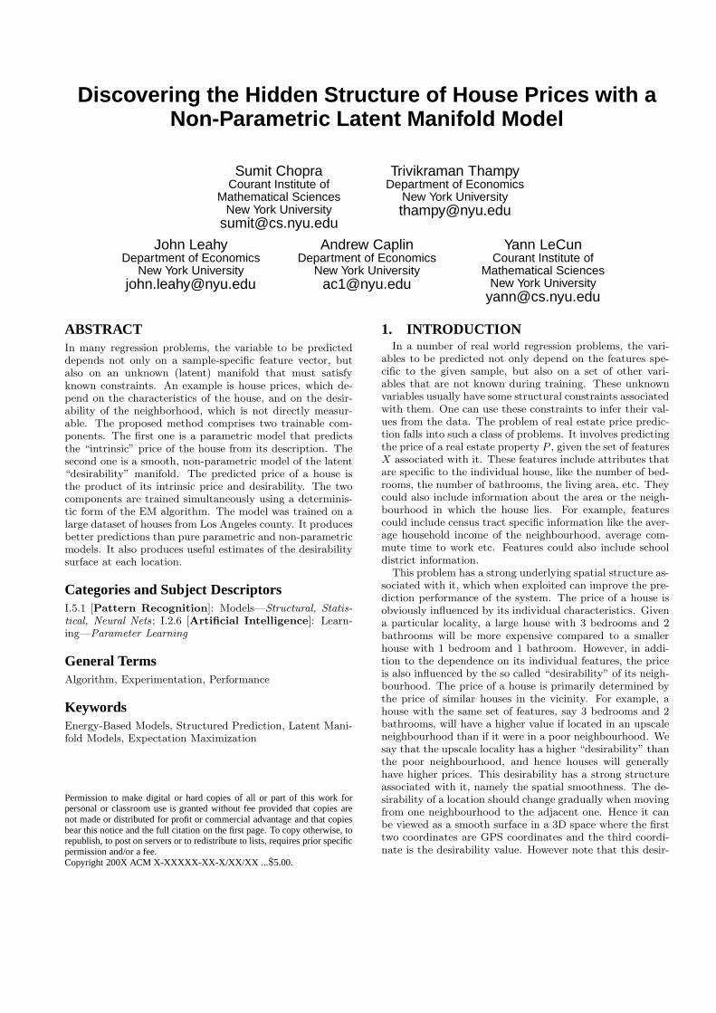
G(W,X)H(D,X)

J(m,h)

X Y

hm

p

F(Y, p)

E(W,D, Y, X)

D

Figure 1: The regression model is composed of twolearning modules: the parametric model G(W, X)and the non parametric model H(D,X).

such as the number of bedrooms, number of bathrooms etc.The full list of house specific features that were used in theexperiments is discussed in section 3. The architecture ofthe model is shown in figure 1. It consists of two trainablecomponents. The first component is the parametric functionG(W, X), parameterized with W , that takes X as input andproduces an output m = G(W,X). This output can be in-terpreted as the “intrinsic price” of the sample. Other thandifferentiability with respect to W , no restriction is imposedon the form/architecture of this function. For the houseprice prediction application, the function G(W, X) was afully connected neural network with two hidden layers.

The second component H(D, X) models the latent man-ifold and is non-parametric in nature. In the light of houseprice prediction, as pointed out in the previous section, theprice of the house P with a set of features X, is stronglyaffected by the “desirability” of its neighbourhood. This“desirability” (which can be viewed as a smooth manifoldspanning the concerned geographic region) is modeled byassigning a “desirability coefficient” di to each training sam-ple Xi. One can interpret the value of the coefficient di asa number specifying how desirable the location of the housethat corresponds to Xi is. The higher the value, the moredesirable it is. Since the value of these coefficients is notknown during training and should be learned, one can viewthese coefficients as the latent variables associated with themodel. For a detailed discussion of latent variable energy-based architectures refer to [15]. Denote by D = [d1, . . . , dn]the vector of all such desirabilities. The hidden desirabilitymanifold is modeled by the desirability vector D and thenon-parametric model H(D, X). This function takes as in-put the sample X (not necessarily a training sample) and thedesirability vector D and produces an output h = H(D, X),which gives the estimate of the desirability of the locationof sample X as a function D. How this estimate is com-puted plays a crucial role in the performance of the system.Hence one must take special care while designing H(D, X).

In the present paper, two versions were used: one was a sim-ple kernel-based interpolating function and the other was aweighted local linear regression model.

2.1.1 Kernel Based InterpolationFor a sample X, let N (X) denote the set of indices of K

training samples that are closest to X (according to somepre-determined similarity measure), for some K. Then theoutput h of the function H(D, X) is given by

h = H(D, X) =X

j∈N (X)

Ker(X,Xj) · dj

. (1)

The kernel function Ker(X, Xj) is defined as

Ker(X, Xj) =

e−q||X−Xj ||2

P

j∈N (X) e−q||X−Xk||2, (2)

with q a constant.

2.1.2 Weighted Local Linear RegressionAnother method used for computing the output of the

function H(D, X) involves fitting a weighted local linear re-gression model in the set of neighbouring training samplesto the sample X. Let α be the parameter vector and β bethe bias of the local linear model. Then fitting a weightedlocal linear model in the set of neighbouring training sam-ples, amounts to finding the parameters α∗ and the bias β∗,such that

(β∗, α

∗) = arg minβ,α

X

j∈N (X)

(dj − (β + αXj))2Ker(X,X

j).

(3)The function Ker(X, Xj) could be any parametric kernelappropriate to the problem. However the one used for theexperiments was the same as the one given in equation 2.Then the solution to the system (or the output of the func-tion H(D, X)) is given by

h = H(D, X) = β∗ + α

∗X. (4)

Remark 1. Even in this case the output h of the func-tion H(D, X) for a sample X can be expressed as a linearcombination of the desirabilities dj of the training samplesXj that lie in the neighbourhood of X, such that the linearcoefficients do not depend on the desirabilities. That is

h = H(D, X) =X

j∈N (X)

ajd

j. (5)

The outputs m and h are combined using a function J toget the prediction of the input sample X. Particularly inthe present paper, instead of predicting the actual prices ofthe houses, the model predicts the log of the prices. Thisallows us to combine the intrinsic price m predicted by theparametric model G(W,X) and the desirability coefficient h

predicted by the non-parametric model H(D,X) additively,rather than multiplicatively. Thus the function J takes thesimple form

J(m, h) = J(G(W, X), H(D, X)) (6)

= G(W, X) + H(D,X). (7)

Another advantage of predicting the log of the price insteadof the actual price is that the absolute prediction error inthe log price corresponds to the relative prediction error inthe actual price, which is what we care about.

Finally the discrepancy between the predicted log price p

and the actual log price Y is given by the energy functionE(W,D, Y, X). The energy function used for the experimentwas half of the square of euclidean distance.

E(W,D, Y, X) =1

2(Y − (m + h))2 (8)

=1

2(Y − (G(W,X) + H(D, X)))2. (9)

2.2 The Learning AlgorithmGiven the training set S = {(X1, Y 1), . . . , (Xn, Y n)}, the

objective of the training is to simultaneously find the pa-rameters W and the desirability coefficients D (the latentvariables of the system) such that the sum of the energyover the training set is minimized. This is done by minimiz-ing the following loss function over W and D

L(W, D) =n

X

i=1

E(W,D, Yi, X

i) + R(D) (10)

=

nX

i=1

1

2(Y i − (G(W,X

i) + H(D, Xi)))2 + R(D).(11)

R(D) is a regularizer on D that prevents the desirabilitiesfrom varying wildly, and helps keep the surface smooth. Inthe experiments an L2 regularizer R(D) = r

2||D||2 was used,

where r is the regularization coefficient.The learning algorithm is iterative and can be seen as a

deterministic form of an EM (a coordinate descent method)algorithm, where D plays the role of auxiliary variables. Theidea is to break the optimization of the loss L with respect toW and D into two phases. In the first phase the parametersW are kept fixed and the loss is minimized with respect to D(the expectation phase of EM). The second phase involvesfixing the parameters D and minimizing the loss with respectto W (maximization phase of EM). The training proceeds byiterating through each of the two phases alternatively untilconvergence. We now explain the details of the two trainingphases for the experiments in this paper.

Phase 1 It turns out that the loss function given by equa-tion 10 is quadratic in D and the process of minimizing itreduces to solving a large scale sparse quadratic system. As-sociate with each training sample Xi a vector U i of size n(equal to the number of training samples). This vector isvery sparse and has only K non zero elements, whose in-dices are given by the elements of the neighbourhood setN (X). The value of the jth non-zero element of this vectoris equal to the linear coefficient that is multiplied with thedesirability dj while estimating the desirability of X. Thus,when the kernel based interpolation is used (equation 1) thenit is equal to Ker(X, Xj), and when local linear regressionmodel is used (equation 5) then it is aj . The loss function(see Equation 10) for this phase can now be written as thefollowing sparse quadratic program

L1(D) =r

2||D||2 +

1

2

nX

i=1

(Y i − (mi + DTU

i))2. (12)

There are two things in particular that one should be carefulabout this loss function.

• During the process of training with sample Xi, wemust interpolate its desirability hi using the desirabil-ities of the training samples whose indices are given by

the set N (Xi). However, special care must be taken toensure that the index of the sample Xi itself is removedfrom the set N (Xi). Not doing so can result in a sys-tem that trivially sets the desirability of each trainingsample equal to the price to be predicted. This wouldmake loss equal to zero, but lead to poor predictions.

• The regularization term plays the crucially importantrole of ensure that the surface be smooth. Without it,the system would overfit the training data and learn ahighly-varying surface, leading to poor predictions.

Another possible modification to the loss given in equa-tion 12, includes an explicit self-consistency term. The ideais to have an explicit constraint that will drive the esti-mate hi of the desirability of training sample Xi given byhi = DT U i to its assigned desirability di. Note that theestimate hi does not involve the term di. Hence the lossfunction now becomes

L1(D) =

r1

2||D||2+

1

2

nX

i=1

(Y i−(mi+DTU

i))2+r2

2

nX

i=1

(di−DTU

i)2.

(13)

Here r1 and r2 are some constants. This loss function is stilla sparse quadratic program and can be solved in the sameway as above.

The above systems can be solved using any sparse sys-tem solvers. However, instead of using a direct method weresorted to iterative methods. The motivation was that ateach iteration of the algorithm, we were only interested inthe approximate solution of the system. We used the conju-gate gradient method with early stopping (also called partialleast squares). The conjugate gradient was started with apre-determined tolerance which was gradually lowered untilconvergence.

Phase 2 This phase involves updating the parameters Wof the function G(W,X) by running a standard stochasticgradient decent algorithm for all the samples (Xi, Y i) in thetraining set, keeping D fixed. For a sample Xi the forwardpropagation was composed of the following steps. Run Xi

through the function G to produce the log of the intrinsicprice mi = G(W,Xi). Interpolate the desirability hi of Xi

from its neighbours using the function hi = H(D, Xi). Addthe desirability to the intrinsic price to get the predictionpi = mi + hi. Compare the predicted value pi with theactual value Y i to get the energy E(W,D) = 1

2(Y i − pi)2.

Finally, the gradient of the energy with respect to W is com-puted using the back propagation step and the parametersW are updated. Here again, we do not train the system tocompletion, but rather stop the training after a few epochs.

The algorithm for training the latent manifold model issummarized in algorithm 1.

2.3 The Testing AlgorithmTesting the input sample X involves a single forward prop-

agation step through the system to compute the predictedprice p = m + h = G(W,X) + H(D, X), using the learnedparameters W and the manifold variables D. This predic-tion is compared with the desired value Y to get the erroron the current sample. The exact measure of error used wasthe Absolute Relative Forecasting error and is discussed insection 4.

3. EXPERIMENTSThe model proposed in this paper was trained on a very

large and diverse dataset. In this section we describe thedetails of the dataset. In addition, we also discuss the detailsof the various standard techniques that have been used forthe problem, with which the performance of the model wascompared. The results of the various techniques are givenin the next section.

3.1 The DatasetThe dataset used was obtained from First American. The

original dataset has around 750,000 transactions of single-family houses in Los Angeles county. The transactions rangefrom the year 1984 to 2004. The dataset has a very hetero-geneous set of homes spread over an area of more than 4000sq miles, with very different individual characteristics. Eachhouse is described by a total of 125 attribute variables. Theattributes specific to the home include, number of bedrooms,bathrooms, the living area of the house, the year built, thetype of property (single family residence etc), number ofstories, number of parking spaces, presence of a swimmingpool, number of fire places, type of heating, type of air con-ditioning, material used for making the foundations etc. Inaddition to this, there are financial attributes including thetaxable land values. Each house is also labeled with a set ofgeographic information like its mailing address, the censustract number, and the name of the school district in whichthe house lies.

In our experiments, we only considered the transactionsthat took place in the year 2004. For the homes transact-ing in 2004, the three geographic fields were used to appendneighborhood and GPS (latitude and longitude) informa-tion to the database. First, the mailing address was used toextract GPS co-ordinates for each home. For neighborhoodinformation, we used the year 2000 census tape. For eachcensus tract in our database, we used data on median house-hold income, proportion of units that are owner-occupied,and information on the average commuting time to work.Finally, we used the school district field for each home toadd an academic performance index (API) to the database.

The dataset is diverse even in terms of the neighbourhoodcharacteristics with transactions spreading across 1754 cen-

Algorithm 1 LME Trainer

Input: training set S = {(Xi, Y i) : i = 1 to N}Initialization: W to random values and D to 0repeat

Phase 1Fix the value of WSolve the quadratic program using conjugate-gradientmethod with early stopping to get a new value of DPhase 2Fix the value of D

for i = 1 to N doMake a forward pass through the model to computethe energyMake a backward pass to compute the gradients ofenergy with respect to WUpdate the parameters W

end foruntil convergence

sus tracts and 28 school districts.The smallest census tractshave as few as 1 transaction, while the biggest census tracthas 350 transactions. The biggest school district in Los An-geles county is Los Angeles Unified with 25,251 transactions.Other school districts have between 200 and 1500 transac-tions.

Out of the numerous house specific and neighbourhood-specific attributes associated with each house, we only con-sidered number of bedrooms, number of bathrooms, yearof construction, living area, median house hold income, em-ployment accessibility index, proportion of units owner occu-pied, and the academic performance index (API). All thosehouses that had missing values for at least one or more ofthese attributes were filtered from the data. In addition,only single family residences were considered. After the fil-tering, there were a total of 70,816 labeled houses in thedataset. Out of these, 80% of them (56,652 in total) wererandomly selected to be used for training purpose and theremaining 20% (14,164) were used for testing.

3.2 The Latent Manifold ModelThe training and testing of the model was done in the way

described in the previous section. The function G(W,X)was chosen to be a 2 hidden layer fully connected neuralnetwork. The first hidden layer had 80 units, and the sec-ond hidden layer had 40 units. The network had 1 out-put unit that gave the “intrinsic price” of the house. Forthe function H(D, X), both the modeling options - kernelsmoothing, and weighted local linear regression - were tried.In the case of kernel smoothing, the value of K, which givesthe size of the neighbourhood set N (X), was chosen to be13. The motivation behind such a choice was the fact thatthe K nearest neighbour algorithm for the problem, gave thebest performance with 13 neighbours. When weighted locallinear regression model was used, K was set to 20. Thisis because the local linear regression model, when ran onthe dataset directly, performed best when the size of theneighbourhoods was 20. The optimization of the quadraticloss function (see Equation 12) was done using the conjugategradient method with early stopping. The idea is to stop theoptimization once the residual of the linear system reaches apre-determined threshold. The value of the threshold is de-creased gradually as a function of the number of iterations ofthe training algorithm. A number of experiments were per-formed using different values of the regularization coefficientr and the factor q in the kernel function. A variation of thequadratic loss that involved an additional explicit smooth-ing term (Equation 13) was also tried. Experiments weredone with a number of different values of the coefficients r1

and r2. The results are reported for the best combinationof values of these coefficients.

3.3 Other Models Used for ComparisonThe performance of the proposed model was compared

to a number of standard techniques that have been in useto solve this problem. We now briefly give a description ofthese techniques.

3.3.1 K - Nearest NeighbourIn this technique, the process of predicting the price of the

sample X involves finding the K nearest training samples(using some similarity measure) and computing the averageprice of these neighbours. Two different similarity measures

were tried. One measure was a euclidean distance in theinput space, where the input consisted of only house spe-cific features and no neighbourhood information like GPS,school district information, and census tract information.The other measure was also a euclidean distance but withthe input having both the house specific and neighbourhoodspecific information. Experiments were done with differentvalues of K and results for the best value are reported.

3.3.2 Regularized Linear RegressionIn the process of regularized linear regression we try to fit

a single linear model on the entire data set without consid-ering the inherent local structure that is associated with it.This is done by minimizing the following objective function

R(W ) =r

2||W ||2 +

1

2n

NX

i=1

(Y i − WTX

i)2. (14)

In this equation W are the parameters to be learned and ris the regularization coefficient.

3.3.3 Box-Cox TransformationAn extenstion of the linear regression is the Box-Cox trans-

form of the linear regression [3], which while maintaining thebasic structure of the linear regression, allows for some non-linearities. The quadratic Box-Cox transform of the hedonicequation is given by

P(θ) = α0 +

kX

i=1

αiZ(λi)i +

1

2

kX

i=1

kX

j=1

γijZ(λi)i Z

(λj)

j . (15)

P is the price, Zi are the attributes, and P (θ) and Z(λi)i

are the Box-Cox transforms.

P(θ) =

P θ − 1

θ, θ 6= 0 (16)

= ln(P ), θ = 0 (17)

Z(λi)i =

Zλii − 1

λi

, λi 6= 0 (18)

= ln(Zi), λi = 0 (19)

All popularly used functional forms in the literature fromlinear (θ = 1), semi-log (θ = 0), log linear (θ = 0, λ = 0,γij = 0), and translog (θ = 0, λ = 0) etc. are all specialcases of the above equation. The above system is first solvedfor the optimal parameters using a combination of maximumlikelihood estimation and grid search on the training data.

3.3.4 Weighted Local Linear RegressionApart from the nearest neighbour method, the above meth-

ods ignore the local structure that is inherent to the problemof house price prediction. The motivation behind using lo-cal regression models is to exploit such a local structure andimprove upon prediction. In weighted local linear regres-sion models, in order to make a prediction for a sample X,a separate weighted linear regression model is fitted usingonly those training samples that are neighbours (in inputspace) to the sample X. The weights are obtained from anappropriately chosen kernel function. For a sample X, ifN (X) gives the indices of the neighbouring training sam-

ples, then the loss function that is minimized is

minβ(X)

X

i∈N (X)

Kλ(X, Xi)[Y i − β(X)f(Xi)]2. (20)

In the above loss β(X) are the regression parameters thatneeds to be learned, f(Xi) is some polynomial function ofXi, and Kλ(X, Xi) is an appropriately chosen kernel widthparameter λ. Once minimized, the prediction P of the sam-ple X is given by

P = β(X) · f(X). (21)

A variation of this model, called the Varying Coefficient

Model (VCM) provides the flexibility of choosing the at-tributes from the input space that are to be used for regres-sion. The idea is to pick two subsets of attributes of theinput sample X. The first subset X1 is used to make a pre-diction, while the second subset X2 is used to determine theneigbors. The following loss function is minimized:

minβ(X2)

X

i∈N (X)

Kλ(X1, Xi1)[Y

i − β(X2)f(Xi1)]

2. (22)

We used this model to study the variation of prediction er-rors as a function of attributes, by trying a number of dif-ferent combinations. In particular, the model was testedusing only house specific attributes in X1, using differentneighbourhood attributes in X2, like GPS coordinates.

3.3.5 Fully Connected Neural NetworkA fully connected neural network also falls into the class

of architectures that do not explicitly make use of the lo-cation information, which characterizes this type of data.However the motivation behind using such an architectureis to capture some non linearities that are hidden in the re-gression function. A number of architectures were tried, andthe one that achieved the best performance was a 2-hiddenlayer network with 80 units in the first layer, 40 units in thesecond, and 1 unit in the output layer.

LME combines the best of both worlds: since there isno restriction on the function G(W, X), it can be a highlycomplicated non linear function capturing non linearities ofregression function, and at the same time D and H(D,X)model the latent manifold which captures the location in-formation associated with the data.

4. RESULTS AND DISCUSSIONThe performance of the systems was measured in terms of

the Absolute Relative Forecasting error (fe) [8]. Let Ai bethe actual price of the house Pi, and let Pri be its predictedprice. Then the Absolute Relative Forecasting error (fei) isdefined as

fei =|Ai − Pri|

Ai

. (23)

Two performance quantities on the test set are reported;percentage of houses with a forecasting error of less than5%, and percentage of houses with a forecasting error of lessthan 15%. The greater these numbers the better the system.Simply using the root mean square error in this setting is notvery informative, because it is overly influenced by outliers.

A comparison of the performance of various algorithms isgiven in table 1. The second and third columns give theperformance of the algorithms when the location dependent

Table 1: Prediction accuracies of various algorithmson the test set. The second and third columns(“Without Loc”) gives the results when no locationdependent information was used as part of the in-put. The fourth and fifth column (“With Loc”) givethe results when the location dependent information(GPS coordinates, census tract fields and school dis-trict fields) is used in the inputs. The various ver-sions of LME algorithms reported are: (a) LME -kernel : when kernel smoothing is used in H(D, X).(b) LME - llr : when local linear regression is usedin H(D, X). (c) S-LME - llr : when local linear re-gression is used, and in addition to it, an explicitsmoothing constraint in the quadratic loss is used.

Algorithm Without Loc With Loc

< 5% < 15% < 5% < 15%

Nearest Neighbor 25.29 62.81 27.51 68.31

Linear Regression 14.04 40.75 19.99 55.20

Box-Cox 19.00 51.00 - -

Local Regression 24.87 62.89 29.20 70.43

Neural Network 24.60 64.54 27.43 70.10

LME - kernel - - 29.39 71.70

LME - llr - - 29.67 72.06

S-LME - llr - - 29.69 72.15

information, like GPS, census tract information, and schooldistrict information is not used as part of the input to thealgorithm. The fourth and fifth columns give the perfor-mance when the location information is used as part of theinput. Various versions of the LME algorithm were trainedand tested. Three such versions are reported. “LME - ker-

nel” denotes the LME algorithm when kernel smoothing isused to model the function H(D, X) (Equation 1), “LME -llr” means when local linear regression is used (Equation 5),and “S-LME -llr” means that in addition to using local lin-ear regression, an explicit smoothing constraint in the lossfunction is used (Equation 13).

One can clearly see that the LME algorithm outperformsall the other algorithms. The best performing version isthe “S-LME-llr”, which predicts 29.69% of houses within anerror margin of less than 5% and 72.15% of houses withinan error margin of less than 15%.

4.1 Importance of Location Dependent Infor-mation

From the results given in the table, one can concludethat information dependent on the geographic location ofthe house, like its GPS coordinates, fields from census tractdata, and fields from the school district in which the houselies, play a crucial role in predicting its price. All the al-gorithms perform significantly better when used with thesevariables than when used without them.

Another thing that is clear from the table is that it is dif-ficult to fit a single parametric model on the entire dataset.Rather one should try to look for models in the non-parametricdomain that change according to the neighbourhod. This isreflected from the fact that methods like linear regressionperform very badly. Whereas a simple method like the Knearest neighbour, which is a highly local, non smooth, anda non-parametric method does a reasonable job. Addingnon-linearities to the linear model does not help either, as

evident from the marginally better performance of the Box-Cox method over its linear counterpart. The fully connectedneural network, though not a non-parametric method, stillgives good performance because of its highly non linear na-ture. But the fact that a simple local linear regression modelon the entire input space performs better than this neuralnetwork further strengthens our belief that part of the modelshould be non-parametric that should take into account thelocality dependent information.

Moreover, how intelligently the locality dependent infor-mation is used is also crucial in making predictions. For in-stance local linear regression method performs better thanthe non linear neural network. Again, this is so because thismethod fits a separate linear model on the neighbouringsamples for the sample X. It is these samples that are verylikely to have a huge influence on the price of X. Here notethat the term “neighbouring” does not necessarily meanphysical proximity. One could define a neighbourhood spacethat includes physical proximity (GPS coordinates), andarea information (census fields and school fields). Amongall the algorithms, the LME uses the location dependent in-formation in the most sophisticated manner. As mentionedbefore, the price of a house not only depends on its individ-ual characteristics but also on the so called “desirability”of the neighbourhood, which can be modeled as a smoothmanifold. LME models this desirability manifold in a non-parametric manner using the function H(D, X) and the de-sirability coefficients D assigned to each training sample,and learns them from the data. Prediction is done by com-bining the local desirability value obtained from the learnedmanifold with the description of the house (the “intrinsicprice” obtained from the parametric model). This processis very intuitive and highly reflective of the real world situa-tion. From the table one can see that all the versions of LMEperform better than the rest of the algorithms. In particu-lar “LME - llr” performs better than “LME - kernel. Thisindicates that the way the locality dependent information isused is very crucial to the performance of the system. Thebest performance of “S-LME - llr” speaks in favor of smoothdesirability manifolds as opposed to non-smooth ones.

4.2 The Desirability and Sensitivity MapsIn this section we give some discussion that provides in-

sights into the working of LME algorithm and argue thatit is representative of the real world scenario. This claim issupported by providing a number of energy maps of the testsamples which we shall discuss.

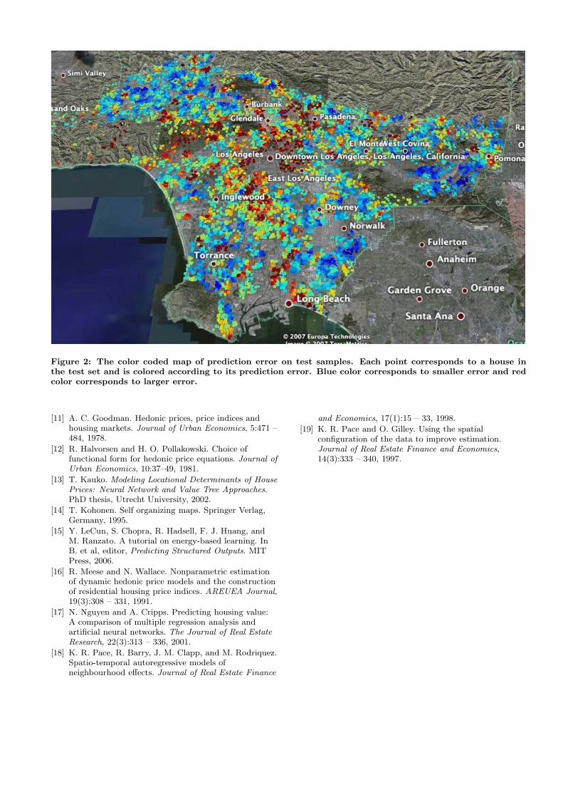
Figure 2 gives the color coded prediction error map on thetest samples. Each point in the figure corresponds to a housein the test sample and is superimposed on top of the satel-lite image of Los Angeles county using its GPS coordinates.The points are colored according to the error in predictionmade by LME. The blue color corresponds to lower predic-tion error and the red color corresponds to higher error. Inorder to make the picture discernible, the color of each pointis smoothed out by assigning it the average color of its 15nearest neighbours. As one can see, the errors made by LMEare not random and seem to have a pattern. In particular,the algorithm does a fairly good job on the out skirts of thecounty. However it is in and around the central part (nearthe downtown area), that it makes a lot of mistakes. Thiscould be attributed to the fact that their is a very high vari-ability in the data around the central part, and the handful

of attributes used in the experiments might not be enoughto capture such a variability.

We also show the desirability map learned by the LMEalgorithm (Figure 3(a)). The map shows the desirabilityestimates of the location of all the houses in the test set.For each test sample, this estimate is computed from thelearned desirabilities D of the training samples and the func-tion H(D,X), as described earlier. The points are coloredaccording to the value of their desirability estimates. Bluecolor implies less desirable and red color implies more desir-able. One can conclude that the value of the desirabilitiesestimated by the algorithm does encode some meaningfulinformation which is a reflection of the real world situa-tion. This is evident from the fact that the areas aroundthe coastline are generally labeled more desirable. Likewise,the areas of Pasadena and near Beverly Hills are also classi-fied as highly desirable. Areas around the downtown area ofthe county, particularly in the south eastern and immediateeast direction, are marked with low desirability.

Finally, we provide some sensitivity analysis; which in-volves measuring the change in the predicted price for asample when the value of one of its attribute is perturbedby a small amount. The motivation behind such an analysisis to check whether the learning algorithm is able to capturein a meaningful way, the non-linearities that are hidden inthe prediction function with respect to the particular at-tribute. For a sample X, the “sensitivity value” SvX asso-ciated with it with respect to some attribute is computed asfollows. First the original price is predicted using the actualvalues of the attributes of X. This is denoted by Prorig.Next, the value of the attribute with respect to which thesensitivity is sought, is increased by one unit. For example,if the attribute is the number bedrooms, then its value is in-cremented by 1. Next the price of the sample X is predictedagain using the same machine parameters but with a per-turbed attribute value. This is denoted by Prpurt. Finallythe “sensitivity value” SvX is computed, which is given by

SvX =Prpurt − Prorig

Prorig

. (24)

The value of SvX can be interpreted as the expected gainin the price of the house when its corresponding attributeis changed by one unit. This information is very importantin solving a seller’s dilemma - whether making certain mod-ification to his/her house before selling would increase itsvalue or not.

The experiments were done using the number of bedroomsas the concerned attribute. For every house in the test set,its number of bedrooms were increased by 1 and the “sensi-tivity value” computed. The results are shown in the formof a color coded map in figure 3(b). The blue color implieslower values of SvX ; which means that the price of the housewill not change by much even when an additional bedroomis added to it. The red color implies higher values of SvX

and indicates that the price of the house will change sub-stantially when a new bedroom is added. From the map, onecan see that the prices in suburban areas of the county arenot as sensitive to an increase in the number of bedroomsas the central (more congested) parts. Thus we concludethat LME indeed is able to capture the correct non-linearrelationship between the number of bedrooms and the priceof the house.

5. CONCLUSIONSIn this paper, we proposed a new approach to regression

for a class of problems in which the variables to be pre-dicted, in addition to depending on features specific to thesample itself, also depend on an underlying hidden manifold.Our approach, called LME, combines a trainable parametricmodel and a non-parametric manifold model to make a pre-diction. We give a novel learning algorithm that learns bothmodels simultaneously. The algorithm was applied to theproblem of real estate price prediction, which falls into sucha class of problems. The performance of LME was comparedwith a number of standard parametric and non-parametricmethods. The advantages of the LME approach was demon-strated through the desirability map and sensitivity map in-fered by the model. These show that the algorithm is indeeddoing something that is a reflection of a real world situation.

Finally, we emphasize that the model proposed here isquite general and can be applied to any regression problemwhich can be modeled as depending upon an underlying non-parametric manifold. The real estate prediction model caneasily extended to include temporal dependencies, so as tolearn a spatio-temporal latent manifold in the GPS+Timespace. Such a manifold would be able to capture the in-fluence on the individual price of a house of neighbourhoodfactors, and also of temporal factors such as local marketfluctuations.

6. ADDITIONAL AUTHORS

7. REFERENCES[1] P. M. Anglin and R. Gencay. Semiparametric

estimation of a hedonic price function. Journal of

Applied Econometrics, 11:633–648, 1996.

[2] S. Basu and T. G. Thibodeau. Analysis of spatialautocorrelation in home prices. Journal of Real Estate

Finance and Economics, 16(1):61 – 85, 1998.

[3] G. E. P. Box and D. R. Cox. An analysis oftransformations. Journal of Royal Statistical Society,B26:211 – 243, 1964.

[4] A. Can. The measurement of neighborhood dynamicsin urban house prices. Economic Geography, 66(3):254– 272, 1990.

[5] A. Can. Specification and estimation of hedonichousing price models. Regional Science and Urban

Economics, 22:453 – 474, 1992.

[6] J. M. Clapp. A semiparametric method for estimatinglocal house price indices. Real Estate Economics,32:127 – 160, 2004.

[7] A. Dempster, N. Laird, and D. Rubin. Maximumlikelihood estimation from incomplete data via the emalgorithm. Journal of Royal Statistical Society, B39:1– 38, 1977.

[8] A. Q. Do and G. Grudnitski. A neural networkapproach to residential property appraisal. Real Estate

Appraiser, 58(3):38 – 45, 1992.

[9] R. A. Dubin. Spatial autocorrelation andneighborhood quality. Regional Science and Urban

Economics, 22:432 – 452, 1992.

[10] A. E. Gelfand, M. D. Ecker, J. R. Knight, and C. F.Sirmans. The dynamics of location in home prices.Journal of Real Estate Finance and Economics,29(2):149 – 166, 2004.

Figure 2: The color coded map of prediction error on test samples. Each point corresponds to a house inthe test set and is colored according to its prediction error. Blue color corresponds to smaller error and redcolor corresponds to larger error.

[11] A. C. Goodman. Hedonic prices, price indices andhousing markets. Journal of Urban Economics, 5:471 –484, 1978.

[12] R. Halvorsen and H. O. Pollakowski. Choice offunctional form for hedonic price equations. Journal of

Urban Economics, 10:37–49, 1981.

[13] T. Kauko. Modeling Locational Determinants of House

Prices: Neural Network and Value Tree Approaches.PhD thesis, Utrecht University, 2002.

[14] T. Kohonen. Self organizing maps. Springer Verlag,Germany, 1995.

[15] Y. LeCun, S. Chopra, R. Hadsell, F. J. Huang, andM. Ranzato. A tutorial on energy-based learning. InB. et al, editor, Predicting Structured Outputs. MITPress, 2006.

[16] R. Meese and N. Wallace. Nonparametric estimationof dynamic hedonic price models and the constructionof residential housing price indices. AREUEA Journal,19(3):308 – 331, 1991.

[17] N. Nguyen and A. Cripps. Predicting housing value:A comparison of multiple regression analysis andartificial neural networks. The Journal of Real Estate

Research, 22(3):313 – 336, 2001.

[18] K. R. Pace, R. Barry, J. M. Clapp, and M. Rodriquez.Spatio-temporal autoregressive models ofneighbourhood effects. Journal of Real Estate Finance

and Economics, 17(1):15 – 33, 1998.

[19] K. R. Pace and O. Gilley. Using the spatialconfiguration of the data to improve estimation.Journal of Real Estate Finance and Economics,14(3):333 – 340, 1997.

(a)

(b)

Figure 3: (a). The color coded values of the desirability surface at the location of the test samples. Forevery test sample X, the estimate of its desirability is computed using the function H(D, X) and the learnedvector D and is color coded according to its value. Blue color implies low desirability and red color implieshigh desirability. (b) The color coded map showing the sensitivity of the prices of houses in the test set withrespect to the number of bedrooms. Blue color implies the price of the house is less sensitive to the change(increase) in the number of bedrooms and red color implies that the price of the house is more sensitive toincrease in the number of bedrooms.