Marano et al. Vol. 19, No. 7 /July 2002 /J. Opt. Soc. Am. A 1319
Discrete Green’s methods and their application totwo-dimensional phase unwrapping
Stefano Marano
Dipartimento di Ingegneria dell’Informazione ed Ingegneria Elettrica, Universita degli Studi di Salerno, via PonteDon Melillo, I-84084 Fisciano (SA), Italy
Francesco Palmieri
Dipartimento di Ingegneria dell’Informazione, Seconda Universita degli Studi di Napoli, Casa Reale dell’Annunziata,via Roma 29, Aversa (CE), Italy
Giorgio Franceschetti*
Dipartimento di Ingregneria Elettronica e delle Telecomunicazioni, Universita degli Studi di Napoli ‘‘Federico II,’’via Claudio 21, I-80125 Napoli, Italy
Received August 17, 2001; revised manuscript received December 17, 2001; accepted December 20, 2001
INTRODUCTIONIntegrodifferential relationships, such as Stokes’s andGauss’s theorems and Green’s formulas, are largely usedin several applications such as adaptive optics, opticaland microwave theory, image compensation, and, moregenerally, image processing. Typically, functions are dis-cretized on domains and boundaries defined over squaregrids by replacing integrals with sums and derivativeswith differences. Even though these approaches havebeen demonstrated to work fine on large scales, specificapplications [we refer specifically to two-dimensionalphase unwrapping (2D PhU)] may occasionally requirediscrete tools that rely exclusively on discrete mathemat-ics without continuous-to-discrete transformations thaton small scales may lead to approximations that are dif-ficult to control.
In this paper, we propose a fully self-contained frame-work in which discrete versions of the above-mentionedtheorems hold rigorously as long as domains and contoursare defined according to a set of specific rules. The de-veloped theory highlights in a rigorous way the peculiari-ties of the discrete method with respect to the continuousone and focuses on some important issues that are to beconsidered if a precise formulation of the discrete problemis required.
These issues include the following:
• Definition of line integrals (sums) on sets composedof aligned pixels.
• Definition of arbitrarily shaped integration domainscomposed of sets of pixels, as emerging from image seg-mentations.
• Definition of test functions (Green’s functions) forapplications of a discrete version of Green’s methods.
• Constraints on the test functions on arbitrary sub-sets of the domain boundary.
The paper is divided into two parts. In Part I, SectionA develops the discrete framework in detail, while the dis-crete equivalents of continuous Green’s functions andtheorems are considered in Section B. In Part II, the ap-plication of the method to 2D Ph-U is presented. Finally,our main conclusions are summarized. Some algebra ispostponed to Appendix A, while details of test functioncomputation are given in Appendix B. A generalizationof the Green’s-function construction, under additionalproblem constraints, is provided in Appendix C.
PART IA. Discrete FrameworkLet us begin, as shown in Fig. 1, by defining our coordi-nate system. We adopt the convention (common in imageprocessing and matrix algebra) of placing the coordinateorigin at the top-left corner. The horizontal axis corre-sponds to the discrete coordinate p, and the vertical onecorresponds to q. Note that, even though we confine our-
2002 Optical Society of America
1320 J. Opt. Soc. Am. A/Vol. 19, No. 7 /July 2002 Marano et al.
selves to two dimensions, the third direction z 5 x 3 y isintroduced for formal completeness.
Scalar functions (or 2D sequences) f( p, q) are definedon the 2D lattice $( p, q)%, as well as vector functionsf( p, q) 5 fx( p, q)x 1 fy( p, q)y.
1. Discrete Differentiation and IntegrationThe first building blocks of our discrete formulation arethe first-order differences:
Dxf~ p, q ! , f~ p, q ! 2 f~ p 2 1, q !, (1)
Dyf~ p, q ! , f~ p, q ! 2 f~ p, q 2 1 !. (2)
We adopt the simplest and most straightforward defi-nitions, even though other versions are obviously pos-sible: For example, operators such as Dxf( p, q)5 c1f( p 1 1, q) 1 c0f( p, q) 1 c21f( p 2 1, q) can bedesigned with a choice for the coefficients ci that satisfiessymmetry, best approximation to the derivative, robust-ness against noise, etc.1 However, our concern in this pa-per is to maintain simplicity and, above all, processing atthe highest resolution, i.e., at the level of the single pixel.This may be crucial in many applications such as PhU,where a loss of resolution may be the immediate conse-quence of the span of the difference-operator definition.Therefore the above choice of two-point differences ap-pears to be convenient, or even imperative, even though itwill force us to construct domains and paths of integra-tion in a slightly asymmetrical way, as will be shown inthe following. Note also that in Eqs. (1) and (2) we usecausal operators, but the dual choice Dxf( p, q) 5 f( p1 1, q) 2 f( p, q) would also lead to a similar frame-work.
Equations (1) and (2) are the first building blocks to de-fine discrete gradient, divergence, and curl operators.All these definitions, as well as those introduced below,are summarized in Table 1 for easier reference (more com-ments about each definition will be given in the follow-ing).
Our next concern in building a discrete theory is to con-sider the discrete counterpart of line integrals. Integra-
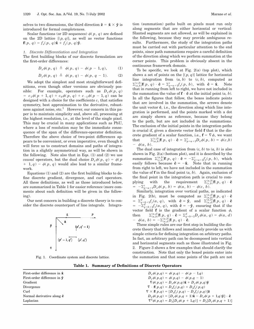
Fig. 1. Coordinate system and discrete lattice.
tion (summation) paths built on pixels must run onlyalong segments that are either horizontal or vertical:Slanted segments are not allowed, as will be explained inthe following, because they may provide ambiguous re-sults. Furthermore, the study of the integration pathsmust be carried out with particular attention to the endpoints, since path summations require a careful definitionof the direction along which we perform summation at thecorner points. This problem is obviously absent in thecontinuous framework domain.
To be specific, we look at Fig. 2(a) (top plot), whichshows a set of points on the $( p, q)% lattice for horizontalline integration from (a, b) to (c, b), computed as( (a,b)
(c,b) f( p, q) • c 5 (p5a11c fx( p, b), with c 5 x. Note
that in running from left to right, we have not included inthe summation the value of f • c at the initial point (a, b).In all the figures that follow, the boxes indicate pointsthat are involved in the summation, the arrows denotethe unit vector c, i.e., the direction along which line inte-gration is performed, and the points marked with a dotare simply shown as reference, because they belongto the path, but are not included in the summations.The exclusion of the initial points in the integration pathsis crucial if, given a discrete vector field f that is the dis-crete gradient of a scalar function, i.e., f 5 ¹f, we wantthat ( (a,b)
(c,b) f( p, q) • c 5 (p5a11c Dxf( p, b) 5 f(c,b)
2 f(a, b).The dual case of integration from (c, b) to (a, b) is also
shown in Fig. 2(a) (bottom plot), and it is described by thesummation ( (c,b)
(a,b)f( p, q) • c 5 2(p5a11c fx( p, b), which
easily follows because c 5 2x. Note that in runningfrom right to left, we have not included in the summationthe value of f in the final point (a, b). Again, exclusion ofthe final point in the integration path is crucial to com-plying with the requirement ( (c,b)
(a,b)f( p, q) • c5 2(p5a11
c Dxf( p, b) 5 f(a, b) 2 f(c, b).Similarly, integration over vertical paths, as indicated
in Fig. 2(b), must be computed as ( (a,b)(a,d)f( p, q) • c
5 (q5b11d fy(a, q), with c 5 y, and ( (a,d)
(a,b)f( p, q) • c5 2(q5b11
d fy(a, q), with c 5 2y, ensuring that if thevector field f is the gradient of a scalar function f,then ( (a,b)
(a,d)f( p, q) • c 5 (q5b11d Dyf(a, q) 5 f(a, d)
2 f(a, b) 5 2( (a,d)(a,b)f( p, q) • c.
These simple rules are our first step in building the dis-crete theory that follows and immediately provide us withsimple criteria for defining integration on arbitrary paths.In fact, an arbitrary path can be decomposed into verticaland horizontal segments such as those illustrated in Fig.2. Figure 3 shows a few examples that should clarify theconstruction. Note that only the boxed points enter intothe summation and that some points of the path are not
Table 1. Summary of Definitions of Discrete Operators
First-order difference in x Dxf( p,q) 5 f( p,q) 2 f( p 2 1,q)First-order difference in y Dyf( p,q) 5 f( p,q) 2 f( p,q 2 1)Gradient ¹f( p,q) 5 Dxf( p,q)x 1 Dyf( p,q)yDivergence ¹ • f( p,q) 5 Dxfx( p,q) 1 Dyfy( p,q)Curl ¹ 3 f( p,q) 5 @Dxfy( p,q) 2 Dyfx( p,q)#zNormal derivative along c Dnf( p,q) 5 @Dyf( p,q 1 1)x 2 Dxf( p 1 1,q)y# • cLaplacian ¹2f( p,q) 5 Dx@Dxf( p 1 1,q)# 1 Dy@Dyf( p,q 1 1)#
Marano et al. Vol. 19, No. 7 /July 2002 /J. Opt. Soc. Am. A 1321
included while other points are counted twice (once verti-cally and once horizontally). With these rules, we havealways and exactly
(~a,b !
~c,d !
f~ p, q ! • c 5 f~c, d ! 2 f~a, b !
if f~ p, q ! 5 ¹f~ p, q !. (3)
We would like to stress that Eq. (3), with the givendefinitions for the first-order differences and the rulesto build the integration paths, guarantees that we canrigorously maintain the definition of ‘‘irrotational field’’in the discrete framework: A discrete vector f( p, q)field is irrotational if f( p, q) 5 ¹f( p, q) for some scalarfunction f. In fact, by simple substitution we havethat the curl ¹ 3 f( p, q) 5 @Dxfy( p, q) 2 Dyfx( p, q)#z5 @DxDyf( p, q) 2 DyDxf( p, q)#z 5 0 ;( p, q). Also,the difference equation fy( p, q) 2 fy( p 2 1, q)2 fx( p, q) 1 fx( p, q 2 1) 5 0, applied to a generic dis-crete vector function f, can be used to verify the existenceof a discrete potential function f( p, q) that can be builtby path integration.
2. Discrete Stokes’s TheoremStokes’s theorem can also be translated into a discreteframework. Consider the rectangular path C with cor-
Fig. 2. Horizontal and vertical integration paths. The boxesindicate points that must be included in the summation, and thearrows indicate the direction of integration.
Fig. 3. Examples of integration paths. Note that in the last ex-ample the path is closed, i.e., (a, b) 5 (c, d), and we have cho-sen to run it counterclockwise.
ners in (a, b) (a, d), (c, d), and (c, b), shown in Fig. 4. Bycomputing the line integral of a vector function f alongthis contour path run in the counterclockwise directionand by using the above-defined convention for inclusion/exclusion of points on the path, we have
(C
f~ p, q ! • c 5 (q5b11
d
fy~a, q ! 1 (p5a11
c
fx~ p, d !
2 (q5b11
d
fy~c, q ! 2 (p5a11
c
fx~ p, b !
5 (p5a11
c
@ fx~ p, d ! 2 fx~ p, b !#
2 (q5b11
d
@ fy~c, q ! 2 fy~a, q !#
5 (p5a11
c
(q5b11
d
@Dyfx~ p, q ! 2 Dxfy~ p, q !#
(4)
because fx( p, d) 2 fx( p, b) 5 (q5b11d Dyfx( p, q) and
the minus sign is a minor formal difference with a typicalcontinuous formulation, and it is simply a consequence ofour definition of reference axes.
The domain D on which the double summation must beperformed is the set of points marked with shaded boxesin Fig. 4. Noteworthy in this discrete framework is thatthe definition of the rectangular domain D (shaded boxes)excludes part of the boundary. In particular, from thefigure we see that some points belonging to C (boxes witharrows) do not belong to D. As anticipated, this is anatural consequence of our definition of the first-order dif-ference operators, which imposes an asymmetrical do-main definition. The set of rules for building domainsand paths that can be applied to an arbitrarily shaped setof pixels may appear at first glance somewhat cumber-some. However, if we accept the maximum-resolutiondefinitions (1) and (2), to the best of our knowledge there
Fig. 4. Contour C (marked with arrows to denote the directionalong which the line integral is evaluated) and domain D (shadedboxes) for Stokes’s theorem on a rectangular region.
1322 J. Opt. Soc. Am. A/Vol. 19, No. 7 /July 2002 Marano et al.
is no way to maintain symmetry if we want to ensure thevalidity of canonical integrodifferential (discrete) rela-tionships, such as Eqs. (3) and (5). In any case, as wewill see below, the rules for recognizing domains andboundaries are quite straightforward.
To see how the set of rules applies also to multiply con-nected domains, consider Fig. 5, where two rectangularpaths are shown: The external path has corner points(a, b), (a, d), (c, d), and (c, b); the internal one has cornerpoints (m, n), (r, n), (r, s), and (m, s). The contour C ismade up of two loops, with the inner one run clockwise.The associated domain D is made up by the pointsmarked with shaded boxes. Note that the upper and leftedges of the external loop, as well as the lower and rightparts of the inner loop, do not belong to D. Moreover, thepoint (m, n) is involved in the double summation over Dbut not in the line integral, which is evaluated on C. Alsonote that point (a, b) is never involved.
With the domain D defined as described above, we im-mediately get the discrete Stokes’s theorem:
(C
f~ p, q ! • c 5 (q5b11
d
fy~a, q ! 1 (p5a11
c
fx~ p, d !
2 (q5b11
d
fy~c, q ! 2 (p5a11
c
fx~ p, b !
2 (q5n11
s
fy~m, q ! 1 (p5m11
r
fx~ p, n !
1 (q5n11
s
fy~r, q ! 2 (p5m11
r
fx~ p, s !
5 (p5a11
c
(q5b11
d
@Dyfx~ p, q !
2 Dxfy~ p, q !#
2 (p5m11
r
(q5n11
s
@Dyfx~ p, q !
2 Dxfy~ p, q !#
Fig. 5. Contour C (marked with boxes or dashed boxes, in bothcases containing arrows) and the associated doubly connected do-main D (shaded boxes).
5 (p5a11
c
(q5b11
d
¹ 3 f~ p, q ! • ~2z!
2 (p5m11
r
(q5n11
s
¹ 3 f~ p, q ! • ~2z!
5 (D
¹ 3 f~ p, q ! • ~2z!. (6)
Result (6) can also be proven implicitly, as it is alwayspossible to decompose an arbitrarily shaped domain (suchas that shown in Fig. 5) into rectangular subsets of pixelsand apply relationship (5) to each subset separately, as il-lustrated in Fig. 6. Then the definitions of D and C fordoubly connected or multiply connected domains of arbi-trary shape immediately follow. Figure 7 shows a fewmore examples of contours of general shape, along withthe associated domains.
In summary, the criterion for associating a discrete do-main with a contour is the following: Sum over the ex-ternal boundary counterclockwise and over the internalboundaries clockwise. The enclosed domain must ex-clude the boundaries that span leftward and downwardand include the others.
Note that in running over a given path, every upper-left corner must be excluded from the summation, andhence it does not belong to C. On the other hand, everylower-right corner must be included twice in the line in-tegral, once in the horizontal direction and once in thevertical direction.
The dual problem that may be of interest is the follow-ing: Given a domain D, build the proper contour C. Therules for deriving C from a given D are simply obtained byinspection and result in considering pixels to the left ofvertical domain edges to be span downward if not belong-ing to D and span upward otherwise, and in consideringpixels above the horizontal domain edges to be span left-ward if not belonging to D and span rightward otherwise.
Fig. 6. Example of how the doubly connected rectangular do-main of Fig. 5 is decomposed into rectangular subsets of pixels.For each subset, relationship (5) is applicable, and the appropri-ate definition of D and C, as illustrated in Fig. 5, immediatelyfollows.
Marano et al. Vol. 19, No. 7 /July 2002 /J. Opt. Soc. Am. A 1323
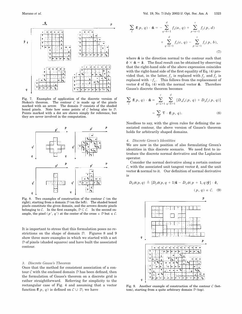
It is important to stress that this formulation poses no re-strictions on the shape of domain D. Figures 8 and 9show three more examples in which we started with a setD of pixels (shaded squares) and have built the associatedcontour.
3. Discrete Gauss’s TheoremOnce that the method for consistent association of a con-tour C with the enclosed domain D has been defined, thenthe formulation of Gauss’s theorem on a discrete grid israther straightforward. Referring for simplicity to therectangular case of Fig. 4 and assuming that a vectorfunction f( p, q) is defined on C ø D, we have
Fig. 7. Examples of application of the discrete version ofStokes’s theorem. The contour C is made up of the pixelsmarked with an arrow. The domain D consists of the shadedboxed pixels. Note how some points of C belong also to D.Points marked with a dot are shown simply for reference, butthey are never involved in the computation.
Fig. 8. Two examples of construction of the contour C (on theright), starting from a domain D (on the left). The shaded boxedpixels constitute the given domain, and the arrows denote pixelsbelonging to C. In the first example, D , C. In the second ex-ample, the pixel ( p8, q8) at the center of the cross P D but ¹ C.
(C
f~ p, q ! • n 5 2 (q5b11
d
fx~a, q ! 1 (p5a11
c
fy~ p, d !
1 (q5b11
d
fx~c, q ! 2 (p5a11
c
fy~ p, b !,
(7)
where n is the direction normal to the contour such thatc 3 n 5 z. The final result can be obtained by observingthat the right-hand side of the above expression coincideswith the right-hand side of the first equality of Eq. (4) pro-vided that, in the latter, fx is replaced with fy and fy isreplaced with 2fx . This follows from the replacement ofvector c of Eq. (4) with the normal vector n. ThereforeGauss’s discrete theorem becomes
(C
f~ p, q ! • n 5 (p5a11
c
(q5b11
d
@Dxfx~ p, q ! 1 Dyfy~ p, q !#
5 (D
¹ • f~ p, q !. (8)
Needless to say, with the given rules for defining the as-sociated contour, the above version of Gauss’s theoremholds for arbitrarily shaped domains.
4. Discrete Green’s IdentitiesWe are now in the position of also formulating Green’sidentities in this discrete scenario. We need first to in-troduce the discrete normal derivative and the Laplacianoperator.
Consider the normal derivative along a certain contourC, with the associated unit tangent vector c, and the unitvector n normal to it. Our definition of normal derivativeis
Fig. 9. Another example of construction of the contour C (bot-tom), starting from a quite arbitrary domain D (top).
1324 J. Opt. Soc. Am. A/Vol. 19, No. 7 /July 2002 Marano et al.
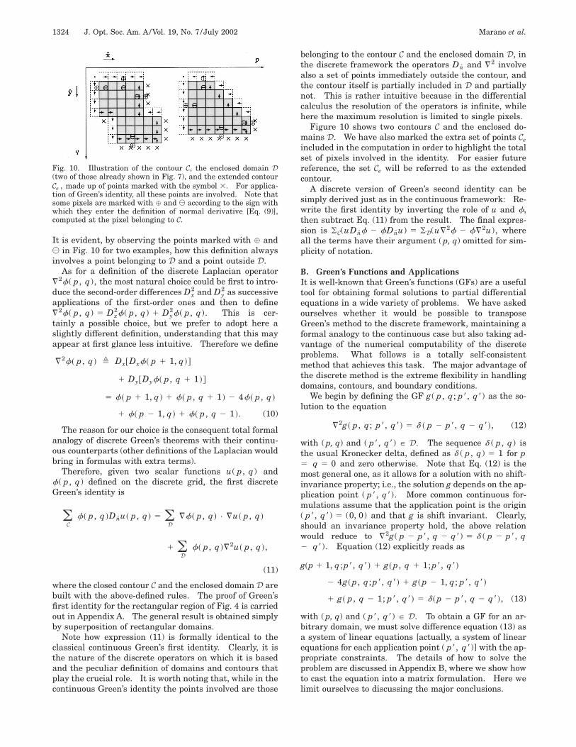
It is evident, by observing the points marked with % and* in Fig. 10 for two examples, how this definition alwaysinvolves a point belonging to D and a point outside D.
As for a definition of the discrete Laplacian operator¹2f( p, q), the most natural choice could be first to intro-duce the second-order differences Dx
2 and Dy2 as successive
applications of the first-order ones and then to define¹2f( p, q) 5 Dx
2f( p, q) 1 Dy2f( p, q). This is cer-
tainly a possible choice, but we prefer to adopt here aslightly different definition, understanding that this mayappear at first glance less intuitive. Therefore we define
¹2f~ p, q ! , Dx@Dxf~ p 1 1, q !#
1 Dy@Dyf~ p, q 1 1 !#
5 f~ p 1 1, q ! 1 f~ p, q 1 1 ! 2 4f~ p, q !
1 f~ p 2 1, q ! 1 f~ p, q 2 1 !. (10)
The reason for our choice is the consequent total formalanalogy of discrete Green’s theorems with their continu-ous counterparts (other definitions of the Laplacian wouldbring in formulas with extra terms).
Therefore, given two scalar functions u( p, q) andf( p, q) defined on the discrete grid, the first discreteGreen’s identity is
(C
f~ p, q !Dnu~ p, q ! 5 (D
¹f~ p, q ! • ¹u~ p, q !
1 (D
f~ p, q !¹2u~ p, q !,
(11)
where the closed contour C and the enclosed domain D arebuilt with the above-defined rules. The proof of Green’sfirst identity for the rectangular region of Fig. 4 is carriedout in Appendix A. The general result is obtained simplyby superposition of rectangular domains.
Note how expression (11) is formally identical to theclassical continuous Green’s first identity. Clearly, it isthe nature of the discrete operators on which it is basedand the peculiar definition of domains and contours thatplay the crucial role. It is worth noting that, while in thecontinuous Green’s identity the points involved are those
Fig. 10. Illustration of the contour C, the enclosed domain D(two of those already shown in Fig. 7), and the extended contourCe , made up of points marked with the symbol 3. For applica-tion of Green’s identity, all these points are involved. Note thatsome pixels are marked with % and * according to the sign withwhich they enter the definition of normal derivative [Eq. (9)],computed at the pixel belonging to C.
belonging to the contour C and the enclosed domain D, inthe discrete framework the operators Dn and ¹2 involvealso a set of points immediately outside the contour, andthe contour itself is partially included in D and partiallynot. This is rather intuitive because in the differentialcalculus the resolution of the operators is infinite, whilehere the maximum resolution is limited to single pixels.
Figure 10 shows two contours C and the enclosed do-mains D. We have also marked the extra set of points Ceincluded in the computation in order to highlight the totalset of pixels involved in the identity. For easier futurereference, the set Ce will be referred to as the extendedcontour.
A discrete version of Green’s second identity can besimply derived just as in the continuous framework: Re-write the first identity by inverting the role of u and f,then subtract Eq. (11) from the result. The final expres-sion is (C(uDnf 2 fDnu) 5 (D(u¹2f 2 f¹2u), whereall the terms have their argument ( p, q) omitted for sim-plicity of notation.
B. Green’s Functions and ApplicationsIt is well-known that Green’s functions (GFs) are a usefultool for obtaining formal solutions to partial differentialequations in a wide variety of problems. We have askedourselves whether it would be possible to transposeGreen’s method to the discrete framework, maintaining aformal analogy to the continuous case but also taking ad-vantage of the numerical computability of the discreteproblems. What follows is a totally self-consistentmethod that achieves this task. The major advantage ofthe discrete method is the extreme flexibility in handlingdomains, contours, and boundary conditions.
We begin by defining the GF g( p, q; p8, q8) as the so-lution to the equation
¹2g~ p, q; p8, q8! 5 d ~ p 2 p8, q 2 q8!, (12)
with ( p, q) and ( p8, q8) P D. The sequence d ( p, q) isthe usual Kronecker delta, defined as d ( p, q) 5 1 for p5 q 5 0 and zero otherwise. Note that Eq. (12) is themost general one, as it allows for a solution with no shift-invariance property; i.e., the solution g depends on the ap-plication point ( p8, q8). More common continuous for-mulations assume that the application point is the origin( p8, q8) 5 (0, 0) and that g is shift invariant. Clearly,should an invariance property hold, the above relationwould reduce to ¹2g( p 2 p8, q 2 q8) 5 d ( p 2 p8, q2 q8). Equation (12) explicitly reads as
g~p 1 1, q;p8, q8! 1 g~ p, q 1 1;p8, q8!
2 4g~ p, q;p8, q8! 1 g~ p 2 1, q; p8, q8!
1 g~ p, q 2 1; p8, q8! 5 d~ p 2 p8, q 2 q8!, (13)
with ( p, q) and ( p8, q8) P D. To obtain a GF for an ar-bitrary domain, we must solve difference equation (13) asa system of linear equations [actually, a system of linearequations for each application point ( p8, q8)] with the ap-propriate constraints. The details of how to solve theproblem are discussed in Appendix B, where we show howto cast the equation into a matrix formulation. Here welimit ourselves to discussing the major conclusions.
Marano et al. Vol. 19, No. 7 /July 2002 /J. Opt. Soc. Am. A 1325
Since the system that results from Eq. (13), as it is, islargely underdetermined, consisting of more unknownsthan equations, various constraint choices are possible, asthey depend on the application that we have in mind.One possibility, which is allowed by the discrete nature ofthe problem, is to calculate a minimum-norm solution orother solutions with more specific boundary constraints.
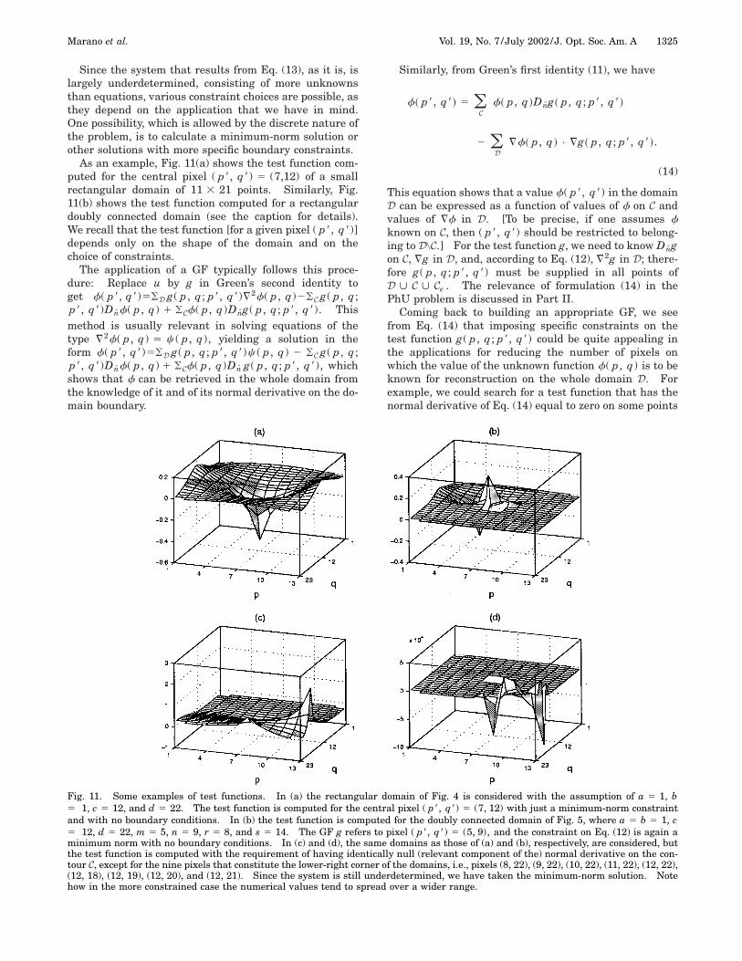
As an example, Fig. 11(a) shows the test function com-puted for the central pixel ( p8, q8) 5 (7,12) of a smallrectangular domain of 11 3 21 points. Similarly, Fig.11(b) shows the test function computed for a rectangulardoubly connected domain (see the caption for details).We recall that the test function [for a given pixel ( p8, q8)]depends only on the shape of the domain and on thechoice of constraints.
The application of a GF typically follows this proce-dure: Replace u by g in Green’s second identity toget f( p8, q8)5(D g( p, q; p8, q8)¹2f( p, q)2(C g( p, q;p8, q8)Dnf( p, q) 1 (Cf( p, q)Dng( p, q; p8, q8). Thismethod is usually relevant in solving equations of thetype ¹2f( p, q) 5 c ( p, q), yielding a solution in theform f( p8, q8)5(D g( p, q; p8, q8)c ( p, q) 2 (C g( p, q;p8, q8)Dnf( p, q) 1 (Cf( p, q)Dn g( p, q; p8, q8), whichshows that f can be retrieved in the whole domain fromthe knowledge of it and of its normal derivative on the do-main boundary.
Similarly, from Green’s first identity (11), we have
f~ p8, q8! 5 (C
f~ p, q !Dng~ p, q; p8, q8!
2 (D
¹f~ p, q ! • ¹g~ p, q; p8, q8!.
(14)
This equation shows that a value f( p8, q8) in the domainD can be expressed as a function of values of f on C andvalues of ¹f in D. [To be precise, if one assumes fknown on C, then ( p8, q8) should be restricted to belong-ing to D\C.] For the test function g, we need to know Dngon C, ¹g in D, and, according to Eq. (12), ¹2g in D; there-fore g( p, q; p8, q8) must be supplied in all points ofD ø C ø Ce . The relevance of formulation (14) in thePhU problem is discussed in Part II.
Coming back to building an appropriate GF, we seefrom Eq. (14) that imposing specific constraints on thetest function g( p, q; p8, q8) could be quite appealing inthe applications for reducing the number of pixels onwhich the value of the unknown function f( p, q) is to beknown for reconstruction on the whole domain D. Forexample, we could search for a test function that has thenormal derivative of Eq. (14) equal to zero on some points
Fig. 11. Some examples of test functions. In (a) the rectangular domain of Fig. 4 is considered with the assumption of a 5 1, b5 1, c 5 12, and d 5 22. The test function is computed for the central pixel ( p8, q8) 5 (7, 12) with just a minimum-norm constraintand with no boundary conditions. In (b) the test function is computed for the doubly connected domain of Fig. 5, where a 5 b 5 1, c5 12, d 5 22, m 5 5, n 5 9, r 5 8, and s 5 14. The GF g refers to pixel ( p8, q8) 5 (5, 9), and the constraint on Eq. (12) is again aminimum norm with no boundary conditions. In (c) and (d), the same domains as those of (a) and (b), respectively, are considered, butthe test function is computed with the requirement of having identically null (relevant component of the) normal derivative on the con-tour C, except for the nine pixels that constitute the lower-right corner of the domains, i.e., pixels (8, 22), (9, 22), (10, 22), (11, 22), (12, 22),(12, 18), (12, 19), (12, 20), and (12, 21). Since the system is still underdetermined, we have taken the minimum-norm solution. Notehow in the more constrained case the numerical values tend to spread over a wider range.
1326 J. Opt. Soc. Am. A/Vol. 19, No. 7 /July 2002 Marano et al.
of C, making the knowledge of the value of f in thosepoints irrelevant. In the most general situation, we maybe interested in forcing a null derivative on arbitrary sub-sets of C. This topic is addressed in Appendix C, with therelevant details for a numerical algorithm. Figures 11(c)and 11(d) are GFs for the same domains and points asthose of Figs. 11(a) and 11(b) but with specific boundaryconditions imposed. See Appendix C and the caption forFig. 11 for more detail and discussion.
In the classical continuous framework, the typical con-straints imposed on GFs are the Dirichlet boundary con-ditions (the test function is set to zero on the boundary),the Neumann boundary conditions (the normal derivativeof the test function is set to zero on the boundary), ormixed Dirichlet–Neumann constraints. The availabilityof a GF is often dependent on analytically complicated orapproximated solutions, such as those based on functionexpansions. In our discrete formulation, we have muchmore flexibility because even though each of the classicalboundary conditions is possible, many other kinds of con-straints may be conceived also at the single-pixel level tocomply with specific application demands. Furthermore,the solution is obtained immediately, and the matrix for-mulation allows us, in any case, to verify that the peculiarconstraints imposed do not result in a linear system thatis overdetermined or impossible.
A question that the reader may ask at this point is howthe discrete Green’s formulation presented here compareswith the classical methods derived in the continuousframework. For space reasons, we cannot report all thecomparisons that we have performed, but we offer somebasic consideration about our findings; the reader is alsoreferred to Ref. 2.
In a continuous framework, GFs, mostly defined onsimply connected domains, are usually built by using ex-pansions on orthonormal bases. We have made severalsimulations on various kinds of domains and constraints,comparing a discretized GF with a totally discrete se-quence derived from our formulation. We have foundthat when the discrete domains are rather large andregular, the differences between a continuous approachand the exact discrete solution are not particularly sig-nificant. However, when the domains are small and/orirregularly shaped (as in the low-coherence PhU problem,to be discussed in the following) the differences may be-come relevant. In these situations, the peculiarities of
the exact discrete method, which often amount to theinclusion/exclusion of a few pixels from the definition ofD, C, and Ce , play an important role in the GF computa-tion and in the function reconstruction. This is also in-tuitive, since for larger domains the contribution of a fewpixels may become less critical.
With the new discrete method, we have also found thatimposing a Dirichlet condition on the boundary of our dis-crete domains always leads to a unique solution for g.We have no proof for this result but only numerical evi-dence. Also, other constraints seem to bring unique so-lutions, but at the moment we can only defer the reader tofuture papers on the topic.
PART IIThe discrete framework developed in this paper may befound useful in various application areas. However, wefind that the 2D PhU problem may be particularly suitedfor taking advantage of such a theory. The PhU problemis somewhat inherently discrete, and we are convincedthat our framework may help to clarify a number of keyissues and lead to better algorithms.
The literature about PhU is now considerably large, asthe problem arises in numerous application fields.3–17
They include image compensation, speckle imaging, adap-tive optics, magnetic resonance imaging, optical and mi-crowave theory, and synthetic aperture radar interferom-etry. For the latter application, several unwrappingmethods have been proposed. We can group themroughly into two main categories: (1) techniques basedon local integration3,4 and (2) techniques based on globaloperators.5–9 In Ref. 13, the connections between globaland local techniques are highlighted, emphasizing thegreater robustness of the latter. As to the global ap-proach, the main formulations can be classified as meth-ods based on the solution of a least-squares (LS) equationand GF-based strategies.
Referring to the former method (LS-based), if we goback to Ref. 8, we see that if the PhU problem is properlystated directly in the discrete time domain, a LS solutioncan be found. It can also be shown that such an ap-proach can be regarded as a discretization of a Poissonproblem, with Neumann boundary conditions. The solu-tion can be based on LS algorithms employing fast trans-form routines, or iterative methods if the additional con-straint of weighted unwrapping is required.9 In Ref. 14,a finite-element method is proposed for discretizing a con-tinuous LS formulation, with the further benefit of beingsuitable for easy inclusion of weighted constraints. Morerecently, a method has been developed in which thewrapped phase is segmented into small blocks that arefirst independently unwrapped and then joined to eachother.15
As to the GF methods, in Ref. 5 a successful approachbased on GFs is proposed. The formulation is developedin a continuous framework, and it is shown to beequivalent16,17 to the LS formulation of Ref. 9. The GFapproach relies on the Green’s identities and has the ma-jor merit of approaching the PhU problem by employingthe background of knowledge and expertise developed inusing the Green’s identities.
Marano et al. Vol. 19, No. 7 /July 2002 /J. Opt. Soc. Am. A 1327
With the analytical framework developed in the previ-ous sections, we are in the position of approaching the 2DPhU problem through the GF approach directly in the dis-crete domain, retaining its advantages and avoidingcontinuous-to-discrete approximations. In fact, with ref-erence to Eq. (14), we have seen that an unknown (phase)sequence f can be recovered on a given domain D fromthe knowledge of its gradient ¹f on D and on the valuesthat f assumes on the contour C. In the PhU problem,¹f is not exactly known, but a corrupted estimate, say fs ,of the vector field can be computed. In this case, as saidabove, it can be shown17 that Eq. (14) with ¹f replaced byfs provides the least-mean-square approximation of thetrue phase f( p, q).
Corruption of the vector field fs can be due to severalreasons: measurement noise, noise ascribed to coherenceloss between the two images used to generate the gradi-ent phase estimate, or undersampling that results inmissing 2p jumps of the true phase. If corrupted areasare preliminarily spotted, then these may be excluded bythe domain D before the phase retrieval is imposed. Theprice that we pay is the absence of reconstruction insidethe excluded areas. In these techniques, our exact for-mulation of the discrete procedure may play an importantrole, because even small areas with crooked contours canbe excluded with confidence.
With these ideas in mind, we now formalize the funda-mentals of the PhU problem starting from the one-dimensional (1D) case and then defining the frameworkfor the 2D phase reconstruction by using solely the dis-crete operators. The PhU topic, already well studied in acontinuous framework, is dealt with in some detail in thebelief that the peculiarity of our exact discrete formalismmay lead to better approximations and algorithms. Inthe following, for simplicity of presentation and for spacereasons, we leave aside the effects of corruption by noise,focusing mainly on the undersampling phenomenon. In-clusion in the discussion of an additive noise term may bestraightforward and is left to future work.
A. One-Dimensional Phase UnwrappingLet us briefly review the PhU problem in one dimension.
Given a phase sequence $f( p)%, with 2` , f( p), ` (true phase), the wrapped phase $fw( p)% is the se-quence of the principal arguments of f( p): fw( p)5 f( p) (mod 2p), with 2p , fw( p) < p. This isequivalent to adding or subtracting to f( p) an integermultiple of 2p: fw( p) 5 f( p) 1 lp2p, lpP $..., 21, 0, 1 ,...%, any time uf( p)u exceeds p. ThePhU problem consists of recovering f( p) from fw( p).
Let us define the 1D finite difference asDf( p) , f( p)2 f( p 2 1). If we limit the variationof f( p) to p, i.e., we impose 2p , Df( p) < p ;p, it iseasy to verify that exact reconstruction of Df( p) fromDfw( p) is obtained with the well-known algorithm
U1@Dfw~ p !#
,H Dfw~ p ! 1 2p if Dfw~ p ! < 2p
Dfw~ p ! if 2p , Dfw~ p ! < p
Dfw~ p ! 2 2p if Dfw~ p ! . p
. (15)
We will refer to the above as the first-order algorithm U1 .The exact phase sequence f( p) can be recovered from theknowledge of f( p8) at an arbitrary point p8 as f( p)5 (k5p811
p Df(k). If such a value is not available, thereconstructed phase will be exact, except for a constantthat must be estimated by other means.
In most practical cases, unfortunately, the condition2p , Df( p) < p is violated at some points, and the re-sult of algorithm U1 is an estimate of Df( p) that differsfrom the true values by multiples of 2p. For a rigorousformulation of the problem, let us define the followingquantities: f( p), true phase; f( p) , Df( p), discretegradient of the true phase; fw( p) P ]2p, p], wrappedphase; fw( p) , Dfw( p), discrete gradient of thewrapped phase; fs( p) 5 U1@ fw( p)#, result of U1 on thegradient of the wrapped phase.
If fs( p) Þ f( p), we say that an undersampling errorhas occurred. We can also write fs( p) 5 f( p)2 s( p)2p, with s( p) 5 21 if 23p , f( p) < 2p, s( p)5 0 if 2p , f( p) < p, s( p) 5 1 if p , f( p) < 3p,s( p) 5 2 if 3p , f( p) < 5p, and so on. More syntheti-cally, s( p): @2s( p) 2 1#p , f( p) < @2s( p) 1 1#p.The sequence $s( p)% is referred to as the undersamplingindex sequence.
B. Two-Dimensional Phase UnwrappingThe above PhU framework can now be extended to the 2Dscenario. With reference to Table 1 and to the coordinatesystem depicted in Fig. 1, we set the following:
• f( p, q), sequence of the true phase;• f ( p, q) 5 fx ( p, q ) x 1 fy ( p, q ) y 5 ¹f ( p, q)
5 Dxf ( p, q) x 1 Dyf( p, q)y, true phase gradi-ent vector field (irrotational);
• fs ( p, q) 5 U1 @ fwx ( p, q) # x 1 U1 @ fwy ( p, q) #y5 fsx ( p, q)x 1 fsy ( p, q)y, vector field obtainedfrom application of algorithm U1 to fw .
In the last expression, the algorithm U1 works on the vari-able p when it is applied to fwx( p, q) and on the variableq when it is applied to fwy( p, q).
As usual, irrotational means that the curl vector isidentically zero. Note that fs is not necessarily irrota-tional, because undersampling errors on each componentof fs may combine to give ¹ 3 fs Þ 0. We can say that if(sampling criteria) 2p , Dxf( p, q) < p and 2p, Dyf( p, q) < p, then the application of U1 is able toreconstruct f ( p, q) 5 ¹f( p, q) from fw( p, q).
The definition of a discrete undersampling vector fieldallows a compact description of the elementary operationinvolved. In fact, we say that in the points wherefs( p, q) Þ f ( p, q), there has been an undersampling er-ror. More specifically, if fsx( p, q) Þ fx( p, q), we havean undersampling error in the x direction [i.e., going frompixel ( p 2 1, q) to ( p, q)]. Similarly, if fsy( p, q)Þ fy( p, q), we have an undersampling error in the y di-rection [i.e., going from pixel ( p, q 2 1) to ( p, q)].Therefore we can write
1328 J. Opt. Soc. Am. A/Vol. 19, No. 7 /July 2002 Marano et al.
fsx~ p, q ! 5 fx~ p, q ! 2 sx~ p, q !2p,
fsy~ p, q ! 5 fy~ p, q ! 2 sy~ p, q !2p, (16)
or fs( p, q) 5 f( p, q) 2 s( p, q)2p, with sx( p, q) andsy( p, q), the undersampling indices, expressed as
sx~ p, q !: @2sx~ p, q ! 2 1#p
, fx~ p, q ! < @2sx~ p, q ! 1 1#p,
sy~ p, q !: @2sy~ p, q ! 2 1#p
, fy~ p, q ! < @2sy~ p, q ! 1 1#p. (17)
The discrete field s( p, q) 5 sx( p, q)x 1 sy( p, q)ycan be taken as a compact representation of the under-sampling errors and will be referred to as the undersam-pling discrete field.
We are now ready to apply our discrete framework tothe PhU problem. Consider the question of detecting un-dersampled areas. An obvious test is to check whetherthe obtained vector field fs [see Eqs. (16)] at each pointis irrotational. If that is not the case, an undersamplingerror must have happened. Unfortunately, the test isnot infallible, and situations with simultaneous ¹3 fs ( p, q) 5 0 and undersampling can arise. Morespecifically, the discrete ¹ 3 operation is ¹ 3 fs( p, q)• z 5 ¹ 3 f ( p, q) • z 2 2p @ sy ( p, q) 2 sy ( p 2 1, q)2 sx( p, q) 1 sx( p, q 2 1)#. Since ¹ 3 f 5 0, we con-clude that ¹ 3 fs( p, q) 5 22p¹ 3 s( p, q). The pointswith an irrotational undersampling vector field will be in-visible to the curl test.
We would like to point out how the definition of an un-dersampling discrete field s( p, q) provides a simple andclear description of the inaccuracies arising from attempt-ing phase reconstruction in the presence of undersampledphase. Hence, when the reconstructed phase fr( p, q) isobtained through path integration on fs rather than on f,we have [the sum is over an arbitrary path C from( pi , qi) to ( p8, q8) with the rules established above]
fr~ p8, q8! 5 (~ pi , qi!
~ p8,q8!
fs~ p,q ! • c
5 (~ pi ,qi!
~ p8,q8!
f~ p,q ! • c
2 2p (~ pi ,qi!
~ p8,q8!
s~ p,q ! • c
5 f~ p8, q8! 2 f~ pi ,qi!
2 2p (~ pi ,qi!
~ p8,q8!
s~ p,q ! • c,
where the unit vector c is the local direction of integra-tion. Therefore the reconstruction error is er( p8,q8)5 22p( ( pi ,qi)
( p8,q8)s( p,q) • c 2 f( pi ,qi). Except for theinitial constant phase term f( pi ,qi), which must beeliminated by other means, the error on the phase is thesum over the contributions given by the undersamplingdiscrete field 22p( ( pi ,qi)
( p8,q8)s( p,q) • c.
It is also possible to use Green’s formulation (14). Ifwe assume that f is perfectly known on C and substitutethe field fs for f, we readily see what happens when thereconstruction of f( p8,q8) is based on the application ofU1 to the measurable field fw :
fr~ p8,q8! 5 (C
f~ p,q !Dng~ p,q; p8,q8! 2 (D
fs~ p,q !
• ¹g~ p,q; p8,q8! (18)
5 f~ p8,q8! 1 2p(D
s~ p,q !
• ¹g~ p,q; p8,q8!, (19)
or er( p8,q8) 5 2p(Ds( p,q) • ¹g( p,q; p8,q8). This ex-pression of the reconstruction error highlights rigorouslythe roles of undersampling field s and test function g inrecovering f( p8,q8). As expected, the error for pixel( p8,q8) is a weighted sum of the undersampling field val-ues, with weights depending on g.
Despite its resemblance with the continuous formulas,we would like to emphasize that expression (18) is notsimply a discretization of continuous operators, but it isan exact relation derived directly from the discrete theory.This also means [see Eq. (19)] that possibly known prop-erties of s could be used to impose constraints on g to con-trol the reconstruction error. Similar considerations mayapply in an enlarged scenario in which noise terms arealso taken into account. These issues suggest, in ouropinion, quite promising further directions of research.
C. Numerical ExampleA numerical example should help in clarifying the appli-cation of the outlined method.
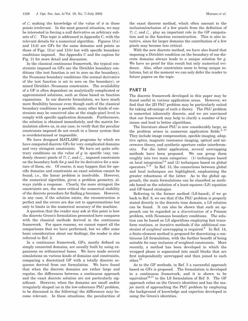
Let us consider a square domain D made of (N 2 1)3 (N 2 1) pixels, with $( p,q): p,q 5 2, 3 ,..., N%,in particular for N 5 9, as in Fig. 12. We know thatthe contour C is to be built with attention to theend points, more specifically as C 5 $(1, q),q 5 2,..., N % ø $( p, 1), p 5 2,..., N% ø $(N,q), q5 2 ,..., N% ø $( p, N), p 5 2 ,..., N%. Furthermore,D ø C 5 $( p,q): p,q 5 1, 2, 3 ,..., N%\$(1, 1)%, and itscardinality is N2 2 1.
Let f( p,q) be the original phase on D ø C, andfw( p,q) its wrapped version, reported in numerical formin each pixel in Figs. 12 and 13, respectively. All the val-ues are given in radians and represent a pyramid with adent in f(5, 2) 5 1.
Assume that f( p,q) is known on C (equal to 1 every-where in this example), while only the wrapped versionfw( p,q) (see Fig. 13) is known in the remaining pixels ofD\(D ù C). The problem is now the recovering of thetrue phase f( p,q) from the measurable field fw( p,q)5 ¹fw( p,q). First, note that uDxf( p,q)u , p ;( p,q),while uDyf( p,q)u , p for all p and q except for the pixel( p,q) 5 (5, 3), where Dyf(5, 3) 5 4.5 rad. After U1is applied, the vector field fs is obtained. We expectan incorrect reconstruction due to the impossibilityfor the algorithm U1 to recover f from fw . In fact, aresult is that fsx( p,q) 5 fx( p,q) ;( p,q), while fsy( p,q)
Marano et al. Vol. 19, No. 7 /July 2002 /J. Opt. Soc. Am. A 1329
5 fy( p,q) ;( p,q) except that fsy(5, 3) 5 21.7832Þ 4.5 5 fy(5, 3). We conclude that the undersamplingfield s has its x component sx identically null and its ycomponent null everywhere, except that sy(5, 3) 5 1.Obviously, in the practical problem, we do not know theactual value of f, and hence we cannot evaluate s. How-ever, in this case, the occurrence of the reconstruction er-ror is detected by the curl test, which gives
Fig. 12. Domain D (shaded boxes) and contour C (depicted asboxes containing arrows indicating the direction according towhich the contour is spanned) for the application of Green’smethod to a square domain. The pixels marked with the symbol3 are those involved in the definition of the test function g butnot belonging to D ø C. On each pixel is shown the value of aphase sequence, with values given in radians. The chosenphase pattern represents a pyramid with a dent at f(5, 2): Ifone substitutes f(5,2) 5 3.25 rad for f(5, 2) 5 1 rad, a perfectpyramidal shape is obtained.
Fig. 13. Example of the wrapped process applied to the 2Dphase sequence of Fig. 12. The PhU problem is the retrieval ofthe original sequence from its (2p, p) determination. All val-ues are given in radians.
¹ 3 fs • z 5 H 22p, ~ p,q ! 5 ~5, 3 !
2p, ~ p,q ! 5 ~6, 3 !
0, elsewhere. (20)
In fact, pixels (5, 3) and (6, 3) are the only ones that in-volves sy(5, 3) when the Dx operator is applied. If wehad to apply Green’s method for recovering the phase ateach pixel ( p8,q8) P D, the error would become
er~ p8,q8! 5 2p(D
s~ p,q ! • ¹g~ p,q; p8,q8!
5 2psy~5, 3 !Dyg~5, 3; p8,q8!
5 2pDyg~5, 3; p8,q8!, (21)
which obviously depends on the test function and spreadsover the whole domain. Using the pseudoinverse methodto obtain the test functions g, as described in Appendix B,we get the reconstruction fr( p,q) shown in Fig. 14.Note also that the value of the error changes from pixel topixel, since different functions g are to be used for differ-ent ( p8,q8).
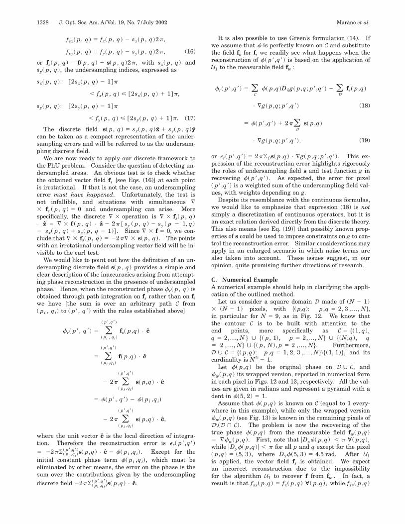
However, since the working example represents a luckycase, because the curl test tells us which point(s) is (are)affected by undersampling, we can simply construct a newdomain excluding the critical points. How can we buildthe new domain? A possible choice is the domain repre-sented by the shaded box of Fig. 15 (with numerical val-ues of the true phase superimposed): Simply cut a por-tion of the initial domain excluding the detectedundersampled pixels. With the new domain is now asso-ciated the contour shown in Fig. 15 as boxes containingone or two arrows. The PhU procedure could be designedstarting from this domain.
The methods developed in this paper allow us to dealwith arbitrarily shaped set of pixels and to limit the a pri-ori knowledge needed to apply the PhU. As a conse-
Fig. 14. Numerical example of phase retrieval procedure bymeans of the proposed unwrapping technique, applied to thephase pattern of Fig. 12, with which the present values should becompared. Note how the error, because of undersampling, hasspread itself over the whole domain D.
1330 J. Opt. Soc. Am. A/Vol. 19, No. 7 /July 2002 Marano et al.
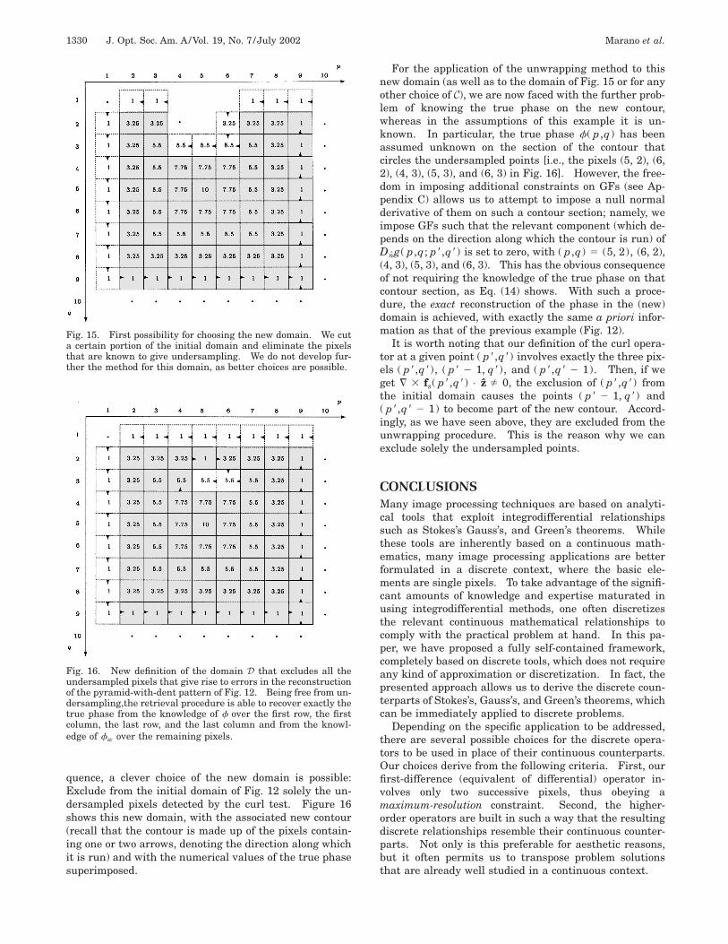
quence, a clever choice of the new domain is possible:Exclude from the initial domain of Fig. 12 solely the un-dersampled pixels detected by the curl test. Figure 16shows this new domain, with the associated new contour(recall that the contour is made up of the pixels contain-ing one or two arrows, denoting the direction along whichit is run) and with the numerical values of the true phasesuperimposed.
Fig. 15. First possibility for choosing the new domain. We cuta certain portion of the initial domain and eliminate the pixelsthat are known to give undersampling. We do not develop fur-ther the method for this domain, as better choices are possible.
Fig. 16. New definition of the domain D that excludes all theundersampled pixels that give rise to errors in the reconstructionof the pyramid-with-dent pattern of Fig. 12. Being free from un-dersampling,the retrieval procedure is able to recover exactly thetrue phase from the knowledge of f over the first row, the firstcolumn, the last row, and the last column and from the knowl-edge of fw over the remaining pixels.
For the application of the unwrapping method to thisnew domain (as well as to the domain of Fig. 15 or for anyother choice of C), we are now faced with the further prob-lem of knowing the true phase on the new contour,whereas in the assumptions of this example it is un-known. In particular, the true phase f( p,q) has beenassumed unknown on the section of the contour thatcircles the undersampled points [i.e., the pixels (5, 2), (6,2), (4, 3), (5, 3), and (6, 3) in Fig. 16]. However, the free-dom in imposing additional constraints on GFs (see Ap-pendix C) allows us to attempt to impose a null normalderivative of them on such a contour section; namely, weimpose GFs such that the relevant component (which de-pends on the direction along which the contour is run) ofDng( p,q; p8,q8) is set to zero, with ( p,q) 5 (5, 2), (6, 2),(4, 3), (5, 3), and (6, 3). This has the obvious consequenceof not requiring the knowledge of the true phase on thatcontour section, as Eq. (14) shows. With such a proce-dure, the exact reconstruction of the phase in the (new)domain is achieved, with exactly the same a priori infor-mation as that of the previous example (Fig. 12).
It is worth noting that our definition of the curl opera-tor at a given point ( p8,q8) involves exactly the three pix-els ( p8,q8), ( p8 2 1, q8), and ( p8,q8 2 1). Then, if weget ¹ 3 fs( p8,q8) • z Þ 0, the exclusion of ( p8,q8) fromthe initial domain causes the points ( p8 2 1, q8) and( p8,q8 2 1) to become part of the new contour. Accord-ingly, as we have seen above, they are excluded from theunwrapping procedure. This is the reason why we canexclude solely the undersampled points.
CONCLUSIONSMany image processing techniques are based on analyti-cal tools that exploit integrodifferential relationshipssuch as Stokes’s Gauss’s, and Green’s theorems. Whilethese tools are inherently based on a continuous math-ematics, many image processing applications are betterformulated in a discrete context, where the basic ele-ments are single pixels. To take advantage of the signifi-cant amounts of knowledge and expertise maturated inusing integrodifferential methods, one often discretizesthe relevant continuous mathematical relationships tocomply with the practical problem at hand. In this pa-per, we have proposed a fully self-contained framework,completely based on discrete tools, which does not requireany kind of approximation or discretization. In fact, thepresented approach allows us to derive the discrete coun-terparts of Stokes’s, Gauss’s, and Green’s theorems, whichcan be immediately applied to discrete problems.
Depending on the specific application to be addressed,there are several possible choices for the discrete opera-tors to be used in place of their continuous counterparts.Our choices derive from the following criteria. First, ourfirst-difference (equivalent of differential) operator in-volves only two successive pixels, thus obeying amaximum-resolution constraint. Second, the higher-order operators are built in such a way that the resultingdiscrete relationships resemble their continuous counter-parts. Not only is this preferable for aesthetic reasons,but it often permits us to transpose problem solutionsthat are already well studied in a continuous context.
Marano et al. Vol. 19, No. 7 /July 2002 /J. Opt. Soc. Am. A 1331
The main peculiarities of the developed discretemethod are in an appropriate definition of the domainsand the contours that are involved in the relationships.That is to say, starting from well-known integrodifferen-tial equations, say the Green’s formulas, if the integralsare replaced with sums, first differences take the place ofderivatives, then exact equivalent discrete equations areobtained, provided that domains (pixels on which thesummations are performed) and boundaries obey somespecific rules. These rules are derived and illustratedwith several examples.
To demonstrate the potential of the discrete method, wehave considered the 2D phase-unwrapping (PhU) ex-ample. For this typical image processing problem, it isseen that many classical PhU techniques based on con-tinuous Green’s formulations may be reformulated,within our discrete framework, without any kind of ap-proximation. Moreover, the intuitions that are behindthe classical methods, as well as their formal elegance,are fully retained. It turns out that the main advantagesof our method are obtained, as one might expect, whenthe application domain is made up of small areas withcrooked contours, as is often the case in phase retrievalbased on measured images that present low-coherenceareas.
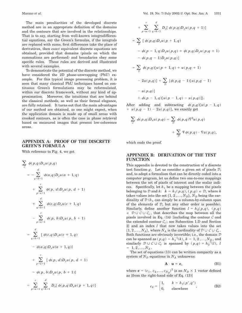
APPENDIX A: PROOF OF THE DISCRETEGREEN’S FORMULAWith reference to Fig. 4, we get
After adding and subtracting f( p,q)@u( p 2 1, q)1 u( p,q 2 1) 2 2u( p,q)#, we exactly get
(C
f~ p,q !Dnu~ p,q ! 5 (D
f~ p,q !¹2u~ p,q !
1 (D
¹f~ p,q ! • ¹u~ p,q !,
which ends the proof.
APPENDIX B: DERIVATION OF THE TESTFUNCTIONThis appendix is devoted to the construction of a discretetest function g. Let us consider a given set of pixels D,and, to adopt a formalism that can be directly coded into acomputer program, let us define two one-to-one mappingsbetween the set of pixels of interest and the scalar indi-ces. Specifically, let h1 be a mapping between the pixelsbelonging to D and k: k 5 h1( p,q), ( p,q) P D, where ktakes values into the set $1, 2 ,..., ND%, ND being the car-dinality of D (h1 can simply be a column-by-column spanof the elements of D, but any other order is possible).Similarly, define another function l 5 h2( p,q), ( p,q)P D ø C ø Ce , that describes the map between all thepixels involved in Eq. (14) [including the contour C andthe extended contour Ce ; see Subsection 1.D and Section2] and an index l that now takes values into the set$1, 2 ,..., NA%, where NA is the cardinality of D ø C ø Ce .Both functions are obviously invertible; i.e., the domain Dcan be spanned as ( p,q) 5 h1
21(k), k 5 1, 2 ,..., ND , andsimilarly D ø C ø Ce is spanned by ( p,q) 5 h2
21(l), l5 1, 2 ,..., NA .
The set of equations (13) can be written compactly as asystem of ND equations in NA unknowns:
A • u 5 c, (B1)
where c 5 (c1 , c2 ,..., cND)T is an ND 3 1 vector defined
as [from the right-hand side of Eq. (13)]
ck 5 H 1, k 5 h1~ p8,q8!
0, elsewhere, (B2)
1332 J. Opt. Soc. Am. A/Vol. 19, No. 7 /July 2002 Marano et al.
u 5 (u1 , u2 ,..., uNA)T is an NA 3 1 vector of the un-
known values of the test function, namely, ul5 g(h2
21(l); p8,q8), l 5 1,2 ,..., NA , and A is the ND3 NA matrix built with all zero entries except for the fiveelements on each row that are described by the followingrelationships [from the left-hand side of Eq. (13)], whereA@i, j# denotes the @i, j# entry of matrix A:
~ p,q ! 5 h121~k !,
A@k, h2~ p 1 1, q !# 5 1,
A@k, h2~ p,q 1 1 !# 5 1,
A@k, h2~ p,q !# 5 24,
A@k, h2~ p 2 1, q !# 5 1,
A@k, h2~ p,q 2 1 !# 5 1,
k 5 1, 2 ,..., ND . (B3)
Equation (B1) represents an underdetermined systemthat admits infinite solutions, provided that the vector cis in the range of A. Any of the infinitely many solutionscan be used as a test function. It is reasonable to choosethe one with minimum norm18,19 as u 5 A1
• c, whereA1 is the pseudoinverse of A.
Note that the resulting test function, contained in u,can be used with the application of Eq. (14) to find thevalue of f in ( p8,q8). In general, a different systemshould be solved to get the test function for each pixel( p8,q8) P D. However, note that in the system (B1) theonly element that depends on ( p8,q8) is the vector c de-fined in Eq. (B2). Therefore each column of A1 containsthe test function for reconstructing a pixel of D. Accord-ingly, the computational cost of the algorithm to build thefunction g is substantially given by a single pseudoiverseoperation. Remember that the evaluation of A1 can bedone off line once and for all, for a given D, dependingonly on the shape of the domain. However, it should bestressed that for very large domains the computationalburden related to the computation of A1 may represent acritical point of the procedure.
Generally, a solution for this problem requires that do-main and contour are such that c is in the range of A, andwe cannot exclude the possibility that, in general, for cer-tain configurations the problem might have no solution.With most types of domains, ranging from rectangular toquite arbitrary shapes, there are no problems.
APPENDIX C: MORE CONSTRAINTS ONTHE TEST FUNCTIONThe method described in Appendix B can be generalizedto impose further constraints on the test function. Inparticular, it is of interest to build test functions with theproperty of having null normal derivatives on arbitrarysubsets of C. Clearly, for any choice of contour, domain,and constraints, we have to verify the existence of a solu-tion for Eq. (13). In fact, as more constraints are im-posed, the system may admit no solution.
To formalize the problem, we denote with T5 $( p,q, d)% the ensemble of points ( p,q) belonging to Cfor which the component of the normal derivative rel-evant to the evaluation of Eq. (14) is to be set to zero, withthe specification of the flag d 5 $horizontal,vertical%, de-noting the direction in which the point ( p,q) is passedover (d 5 horizontal if, for the considered point, c 5 x orc 5 2x, and d 5 vertical otherwise). A given couple( p,q) will be included twice in T (once with d5 horizontal and once with d 5 vertical) if the pixel( p,q) is included twice in the definition of the contour.Let NP be the cardinality of T.
Introduce now the one-to-one mapping h3 between theelements of T and an index j: j 5 h3( p,q, d), ( p,q, d)P T, where j will take values into the set $1, 2 ,..., NP%.Define the enlarged coefficient matrix Ae to be the (ND1 NP) 3 NA matrix whose first ND rows are builtthrough relationships (B3), while the remaining NP rowshave all zero entries except two, which are given by thefollowing rule:
~ p,q, d ! 5 h321~ j !,
Ae@ND 1 j, h2~ p,q 1 1 !# 5 1,
Ae@ND 1 j, h2~ p,q !# 5 21
if d 5 horizontal,
Ae@ND 1 j, h2~ p 1 1, q !# 5 1
Ae@ND 1 j, h2~ p,q !# 5 21
if d 5 vertical,
where j 5 1, 2 ,..., NP . Previous arrangements are eas-ily understood from our definition of the normal deriva-tive Dn , which involves Dy if the point is run horizontallyand Dx for a point passed over in the vertical direction.Define also an augmented version of the vector c given by
with dimension (ND 1 NP) 3 1. This yields a system ofND 1 NP equations in NA unknowns: Ae • u 5 ce ,whose minimum-norm solution is u 5 Ae
1• ce .
Note that while ND , NA , it may happen that ND1 NP . NA . In this case, the problem is overdeter-mined, and Ae
1• ce represents only its LS solution. Ob-
viously, the larger the number NP of additional con-straints, the more critical the inversion of Ae , asconfirmed by the growth of the condition number (ratiobetween the largest and the smallest singular value ofAe), which indicates a numerically ill-posed problem.18,20
In practice, the size and the shape of the initial domain,the points involved in the definition of T, and its size NPall have influence on the numerical tractability of themethod, and a case-by-case study is required. It is alsonecessary to stress that the columns of Ae
1 contain thetest function for all the pixels of D, meaning that a singlepseudoinverse computation of Ae essentially representsthe complexity of the numerical procedure.
To see an example of a test function on which some ad-ditional constraints are imposed, let us look at Figs. 11(c)
Marano et al. Vol. 19, No. 7 /July 2002 /J. Opt. Soc. Am. A 1333
and 11(d), where we consider a rectangular domain and adoubly connected rectangular domain, such as those de-picted, respectively, in Figs. 4 and 5. The test functionsshown are computed by imposing a null relevant compo-nent of the normal derivative on the whole contour C ex-cept for the nine pixels in the lower-right corner of the do-main. If we compare Figs. 11(c) and 11(d) with Figs.11(a) and 11(b), it is clear that the additional require-ments give rise to a less smooth g.
To give an idea of the numerical features involved inthe construction of the test function, we refer to the caseof the singly connected domain. A result is that, by im-posing the (relevant component) null normal derivativecondition on C except for the nine pixels in the lower-rightcorner, we have a matrix coefficient Ae with (ND 1 NP)3 NA 5 285 3 295 having rank 285 and condition num-ber 755.37. If we augment the number of constraints upto imposing the null derivative condition on the whole Cexcept for the single pixel ( p,q) 5 (12, 22), we obtain a293 3 295 matrix coefficient having rank 293 and condi-tion number 963.8. Trying to force to zero the normal de-rivative of the remaining pixel (12, 22) (which is involvedtwice in T) causes Ae to become a 295 3 295 square ma-trix that is not invertible, as it is rank deficient (rank294). In the latter case, the numerical accuracy of the re-trieval procedure for f becomes unpractical.
*Also with the Department of Electrical Engineering,University of California, Los Angeles, California 90024-1594.
REFERENCES1. A. V. Oppheneim and R. W. Schafer, Discrete Time Signal
Processing (Prentice-Hall, Englewood Cliffs, N.J., 1989).2. S. Marano, F. Palmieri, and G. Franceschetti, ‘‘Integral-
differential relationships reformulated for image processingapplications,’’ manuscript in preparation.
3. J. M. Tribolet, ‘‘A new phase unwrapping algorithm,’’ IEEETrans. Acoust., Speech, Signal Process. ASP-25, 170–177(1977).
4. R. M. Goldstein, H. A. Zebker, and C. L. Werner, ‘‘Satellite
radar interferometry: two-dimensional phase unwrap-ping,’’ Radio Sci. 23, 713–720 (1988).
5. G. Fornaro, G. Franceschetti, and R. Lanari, ‘‘Interferomet-ric SAR phase unwrapping using Green’s formulation,’’IEEE Trans. Geosci. Remote Sens. 34, 720–727 (1996).
6. M. D. Pritt and J. S. Shipman, ‘‘Least-squares two dimen-sional phase unwrapping using FFT’s,’’ IEEE Trans. Geosci.Remote Sens. 32, 706–708 (1994).
7. J. L. Marroquin and M. Rivera, ‘‘Quadratic regularizationfunctionals for phase unwrapping,’’ J. Opt. Soc. Am. A 12,2393–2400 (1995).
8. B. R. Hunt, ‘‘Matrix formulation of the reconstruction ofphase value from phase differences,’’ J. Opt. Soc. Am. 69,393–399 (1979).
9. D. C. Ghiglia and L. A. Romero, ‘‘Robust two-dimensionalweighted and unweighted phase unwrapping that uses fasttransforms and iterative method,’’ J. Opt. Soc. Am. A 11,107–117 (1994).
10. G. Fornaro, G. Franceschetti, R. Lanari, and E. Sansosti, ‘‘Atheoretical analysis of the robust phase unwrapping algo-rithms for SAR interferometry,’’ in Proceedings of the IEEEInternational Symposium on Geoscience and Remote Sens-ing (Institute of Electrical and Electronics Engineers, NewYork, 1996), pp. 2047–2049.
11. S. Moon-Ho Song, S. Napel, N. J. Pelc, and G. H. Glover,‘‘Phase unwrapping of MR images using Poisson equation,’’IEEE Trans. Image Process. 4, 667–676 (1995).
12. G. Fornaro, G. Franceschetti, R. Lanari, and E. Sansosti,‘‘Robust phase-unwrapping techniques: a comparison,’’ J.Opt. Soc. Am. A 13, 2355–2366 (1996).
13. G. Fornaro, G. Franceschetti, R. Lanari, E. Sansosti, andM. Tesauro, ‘‘Global and local phase-unwrapping tech-niques: a comparison,’’ J. Opt. Soc. Am. A 14, 2702–2708(1997).
14. G. Fornaro, G. Franceschetti, R. Lanari, D. Rossi, and M.Tesauro, ‘‘Interferometric SAR phase unwrapping using thefinite element method,’’ IEE Proc. Radar Sonar Navig. 144(No. 4), 1–9 (1997).
15. J. Strand, T. Taxt, and A. K. Jain, ‘‘Two-dimensional phaseunwrapping using a block least-square method,’’ IEEETrans. Image Process. 8, 375–386 (1999).
16. D. C. Ghiglia and M. D. Pritt, Two-Dimensional Phase Un-wrapping (Wiley, New York, 1998).
17. G. Franceschetti and R. Lanari, Synthetic Aperture RadarProcessing (CRC Press, Boca Raton, Fla., 1999).
18. R. A. Horn and C. R. Johnson, Matrix Analysis (CambridgeU. Press, Cambridge, UK, 1990).
19. W. H. Press, S. A. Teukolsky, W. A. Vetterling, and B. P.Flannery, Numerical Recipes in C: The Art of ScientificComputing, 2nd ed. (Cambridge U. Press, Cambridge, UK,1993).
20. S. S. Haykin, Adaptive Filter Theory, 3rd ed. (Prentice-Hall,Englewood Cliffs, N.J., 1995).