Discretization Methods for Multiphase Flow Simulation of Ultra-Long Gas-Condensate Pipelines Erich Zakarian, Henning Holm Shtokman Development A.G., Russia Dominique Larrey Total E&P, Process Department, France ABSTRACT As part of the development of the super-giant Shtokman gas field in the Barents Sea, two discretization methods were introduced for the multiphase flow simulation of the 550km- long dry-two-phase gas export pipeline to shore. First, both methods are described in details, with an illustrative application to the Shtokman case. Then, in-depth validation is performed through steady-state flow simulations. The sensitivity to dynamic simulation is also addressed. 1 PROFILE DISCRETIZATION OF GAS-CONDENSATE PIPELINES Multiphase flow simulation of gas-condensate pipelines brings many challenges to the Flow Assurance Engineer. Particularly, given either as-built profile or detailed terrain survey, the actual or expected pipeline geometry must be discretized into a simplified profile to allow reasonable computation time. In case of ultra-long pipelines, this discretization requires the compression of a huge number of data points, typically from several tens of thousand coordinates to only few thousand points. The transformation is therefore significant and must be handled with great care since liquid accumulation in gas-condensate flow is known to be very sensitive to pipe inclination (1). This is particularly true at the design stage of new field development: if discretization is not properly carried out, the onset of liquid accumulation can be under-predicted with respect to gas export flow rate. Possible consequences are: wrong definition of the operating envelope; inappropriate design of receiving facilities; high level trips in slug catcher during transient operations; higher risk of gas flaring; etc.
Transcript
Discretization Methods for Multiphase Flow Simulation of Ultra-Long Gas-Condensate Pipelines
Erich Zakarian, Henning Holm Shtokman Development A.G., Russia Dominique Larrey Total E&P, Process Department, France ABSTRACT As part of the development of the super-giant Shtokman gas field in the Barents Sea, two discretization methods were introduced for the multiphase flow simulation of the 550km-long dry-two-phase gas export pipeline to shore. First, both methods are described in details, with an illustrative application to the Shtokman case. Then, in-depth validation is performed through steady-state flow simulations. The sensitivity to dynamic simulation is also addressed. 1 PROFILE DISCRETIZATION OF GAS-CONDENSATE PIPELINES Multiphase flow simulation of gas-condensate pipelines brings many challenges to the Flow Assurance Engineer. Particularly, given either as-built profile or detailed terrain survey, the actual or expected pipeline geometry must be discretized into a simplified profile to allow reasonable computation time. In case of ultra-long pipelines, this discretization requires the compression of a huge number of data points, typically from several tens of thousand coordinates to only few thousand points. The transformation is therefore significant and must be handled with great care since liquid accumulation in gas-condensate flow is known to be very sensitive to pipe inclination (1). This is particularly true at the design stage of new field development: if discretization is not properly carried out, the onset of liquid accumulation can be under-predicted with respect to gas export flow rate. Possible consequences are: wrong definition of the operating envelope; inappropriate design of receiving facilities; high level trips in slug catcher during transient operations; higher risk of gas flaring; etc.
1.1 Basics The discretization of gas-condensate pipeline profile needs at least to satisfy the following requirements (2):
1. The total pipe length must be preserved.
2. The simplified geometry must have the same overall shape (large and small scale undulations) to induce the same dynamics: propagation of level slugs after restart, formation of large liquid waves during inspection pigging or production ramp-up, gravity-driven flow, etc.
3. The total climb must be conserved to predict the same overall liquid content in steady-state flow conditions. By total climb, we mean the accumulated total length of upward inclined pipes.
4. The angle distribution of the discretized profile must be as close as possible to the original distribution. By angle distribution, we mean the distribution of cumulated pipe length among predefined angle groups.
The last requirement is obviously the most difficult one to achieve. A conventional approach is to predefine inclination classes where elements of relevant sub-profiles will be grouped and lumped together. A commercial solution is available today within the OLGA® Geometry Editor (3). We propose to review this solution before presenting two alternatives. 1.2 OLGA® Geometry Editor When profile simplification is justified, two options are available in OLGA® to filter the geometry of a pipeline: box filter or angle distribution preservation. The first option is mainly intended for removing noise from as-built pipeline survey. In other circumstances, when for example evaluating pressure drop along an existing pipeline with a known profile, box filtering can be used for data compression to speed-up simulation. However box filtering is not at all recommended when liquid content is the parameter under investigation since important details of the pipeline profile are likely to be lost. An instructive demonstration will be given in the last part of this paper. The second option of the Geometry Editor proposes to preserve the first and fourth aforementioned requirements; i.e. conservation of total pipe length and angle distribution. As advised in the user manual of the Geometry Editor, several tries are necessary to select the best candidate (3): it is a good idea to compare the angle distributions of the original geometry and the filtered ones. The filter with the best reproduction of the original geometry should be used; keeping in mind that the angle groups should be representative. From our experience with the Shtokman case, it is extremely difficult or even impossible to satisfy the four aforementioned requirements with this second option. It is also worth reminding that this method is strongly dependent on the selection of relevant angle groups and sub-profiles, making almost impossible to achieve an optimal result without some additional external programming. Though complex and challenging, a discretization satisfying the four aforementioned requirements is deemed mandatory for ultra-long gas-condensate transport systems such
as Shtokman: the seabed of the Barents Sea is indeed characterized by iceberg scours and (elongated) pockmarks, making pipeline profiles extremely rough. To take up this challenge of long and rough pipeline profile discretization, two methods were conceived:
• Based on the concept of pipeline indicator (4), the first method introduces a three-step algorithm for the sequential selection, filtering and complexification of relevant sub-profiles. The result is a series of new pipe coordinates, ready to be entered in a multiphase flow simulator.
• The second method is based on the lumping of elements with similar inclination. The lumped elements are then redistributed to match the large scale and small scale topography of the original profile “as good as possible”.
Unlike conventional approaches, the predefinition of pipe inclination classes (or angle groups) is not required for both methods, thus relieving the Engineer of the most sensitive input. The distribution of pipe inclinations is also better conserved. Both methods will be described through their application to the Shtokman case. A pipeline profile from the Shtokman field to the onshore location of Teriberka, Russia, was derived from a detailed seabed bathymetry survey by Pipeline Engineers, taking account of free span analysis and seabed intervention. The resulting profile, defined by a set of 108,785 points, will be used to illustrate our two discretization methods. This very fine description is appropriate to determine the “roughness” of the pipeline geometry. However it is far too excessive to be directly implemented in a dynamic simulator as we will see in the last part of this paper. 2 PROFILE DISCRETIZATION: FIRST METHOD 2.1 Pipeline indicator The pipeline indicator is a dimensionless parameter which quantifies the propensity of gas-condensate pipelines to accumulate liquid in steady-state flow conditions (4):
( ) ( )[ ]1000
0
1
1 ××−
=
∑
∑
=
=N
ii
N
iii
L
LHoldupHoldupPI
θ
where:
( ) ( )[ ] 25066091490 ...tan.+−×= ii ArcHoldup θ
πθ
θi = inclination of pipe i with respect to horizontal [%] Li = length of pipe i [m] N = number of pipes
The pipeline indicator is based on a fairly simple Holdup correlation. The latter does not pretend to accurately quantify the liquid content within a pipe. It is a simple mathematical correlation which aims to reproduce the typical step-function of the liquid holdup with respect to pipe inclination in gas-condensate flow (5). Note that θi is defined in percent and not in degree in the correlation.
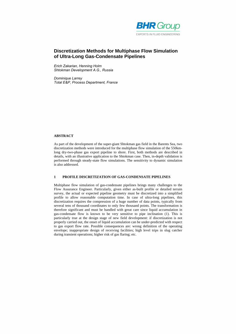
An example is given in Figure 1 where the above Holdup correlation can be compared to the liquid holdup predicted with OLGAS® version 5.3 (6), for representative flowing conditions of the Shtokman gas export to shore.
OLGAS 5.3: liquid holdup vs. pipe inclination and gas superficial velocityUSL=0.003 m/s - ρG=180 kg/m3 - ρo=775 kg/m3 - μG=0.02 cP - μO=2.5 cP
σ=0.0025 N/m - Wall roughness=30 μm - Inner diameter=0.9906 m
Figure 1: Pipeline indicator definition: holdup function
Total E&P experience in gas-condensate pipeline design and operation has led to development of an empirical pipeline indicator scale (4): see Table 1. From the above definition, it was straightforward to calculate the pipeline indicator of the Shtokman gas export to shore. The latter, equal to 79.68, is in the upper range of the scale.
PI value Total E&P experience in gas-condensate pipeline design and operation
PI < 0 The pipeline profile is rather globally sloping downwards. No particular operating problem is expected.
0 < PI < 20 The pipeline profile is close to horizontal or the profile is over-simplified. No particular operating problem is expected.
20 < PI < 40 The pipeline profile is relatively flat (or slightly hilly). Normal operation is not expected to be difficult. Possible problems at very low flow rates or following restart.
40 < PI < 80 The pipeline crosses hilly terrain. Operation (e.g. ramp-up) has to be studied carefully.
80 < PI The pipeline profile is very hilly. Operation requires very careful study. Validity of simulation software to be checked.
Table 1: Pipeline indicator scale (4)
2.2 Discretization Profile discretization is based on the following three steps:
1. Pipeline indicator analysis for the selection of relevant sub-profiles.
2. Simplification of the original sub-profiles.
3. Optimized complexification of the selected sub-profiles.
Note: by complexification, we simply mean roughening by addition of random points along the pipeline profile to make it more irregular or bumpier. 2.2.1 Sub-profile selection In Figure 2, the geometry of the Shtokman pipeline (elevation, total climb, and pipe inclination) is given for the original profile (108,785 points – 554 km).
Figure 2: Original profile (108,785 points): geometry
It is clear that pipe inclination is not evenly distributed along the export route. Some portions are relatively flat like the one around kilometre point (KP) 240 where pipe inclination never exceeds +/- 1°. Some other parts are fairly hilly like the first hundred kilometres where pipe angles can be up to +/-7°. To ease the selection of relevant sub-profiles, the profile of pipeline indicator was calculated at different scales by dividing the pipeline into sub-profiles of constant length: 1, 5, 10, 25, 50 km: cf. Figure 3. With pipeline indicator calculated every 1 km, the selection of consistent sub-profiles is unclear as the indicator varies significantly from one point to another. And vice-versa, a large scale like 50 km over-simplifies the real complexity of the pipeline geometry. An intermediate scale (10 km) seems to be more appropriate to select relevant sub-profiles as shown in Figure 4. The pipeline indicator, total climb and total length were computed for each selected sub-profile: cf. Table 2.
Table 2: Sub-profile selection: pipeline indicator and total climb
-100-50
050
100150200250300
0 100000 200000 300000 400000 500000
Pipe
line
indi
catto
r [-]
Distance from offshore platform [m]
Pipeline indicator
020406080
100120140160
0 100000 200000 300000 400000 500000
Pipe
line
indi
catto
r [-]
Distance from offshore platform [m]
Pipeline indicator
020406080
100120140160
0 100000 200000 300000 400000 500000
Pipe
line
indi
catto
r [-]
Distance from offshore platform [m]
Pipeline indicator
020406080
100120140160
0 100000 200000 300000 400000 500000
Pipe
line
indi
catto
r [-]
Distance from offshore platform [m]
Pipeline indicator
020406080
100120140160180
0 100000 200000 300000 400000 500000
Pipe
line
indi
catto
r [-]
Distance from offshore platform [m]
Pipeline indicator
Figure 3: Pipeline indicator profile at different scales (1, 5, 10, 25, 50 km)
020406080
100120140160180
0 100000 200000 300000 400000 500000
Pipe
line
indi
catto
r [-]
Distance from offshore platform [m]
-10-8-6-4-202468
10
230000 240000 250000 260000 270000 280000
Incl
inat
ion
[deg
]
Distance from offshore platform [m]
Pipe inclination
-10-8-6-4-202468
10
410000 420000 430000 440000 450000 460000
Incl
inat
ion
[deg
]
Distance from offshore platform [m]
Pipe inclination
Figure 4: Sub-profile selection through pipeline indicator analysis
2.2.2 Filtering The selected sub-profiles must now be simplified to condense the original set of 108,785 discretization points into a smaller set. Previous work in the Shtokman project had demonstrated that pipeline discretization with approximately 2,500 pipes (and 2 calculation cells or sections per pipe) was an acceptable upper limit in terms of computation time. This figure provides a target for the simplification process: assuming 2,500 pipes for a 550km pipeline, each pipe length should be about 200 m. The Box Filter available within the OLGA® Geometry Editor is used for filtering: a sample distance of 1000 m is set to pick-up one point every one kilometer from the original profile. This sample distance is large enough to allow the later complexification of the sub-profiles with a sample length of 200 m. It also preserves the overall shape (and most of the low points) of the original profile: cf. Figure 5.
0500100015002000250030003500400045005000
-400
-300
-200
-100
0
100
200
0 100000 200000 300000 400000 500000
Total climb [m
]Elev
atio
n [m
]
Distance from offshore platform [m]
Pipeline geometryPipe elevation (simplified profile with OLGA box filter) [m]Pipe elevation (original profile: 108,785 points) [m]Total climb (original profile: 108,785 points) [m]Total Climb (simplified profile with OLGA box filter) [m]
-15-10
-505
101520
0 100000 200000 300000 400000 500000
Incl
inat
ion
[deg
]
Distance from offshore platform [m]
Pipe inclinationPipe inclination (original profile: 108,785 points) [deg]Pipe inclination (simplified profile with OLGA box filter) [deg]
Figure 5: Profile simplification: new geometry
As expected, the filtering smoothes out the original geometry. The overall pipeline indicator is now 25.8 instead of 80. The total climb is also drastically reduced, now 1,235 m instead of 4187 m. The total length remains approximately the same with 554,400 m instead of 554,505 m. 2.2.3 Complexification So far, the first two requirements listed in section 1.1 are satisfied. The simplified profile must now be complexified to increase the total climb and keep the angle distribution of the discretized profile as close as possible to the original one. This is achieved according to the following constraints:
1. The total climb of each sub-profile must be preserved by +/- 1%. 2. The pipeline indicator of each sub-profile must be preserved by +/-1%. 3. The minimum pipe length must be about 200 m.
A complexification is successively applied to each sub-profile by adding random points along the simplified sub-profile: cf. Figure 6 (left side). Basically, given a sub-profile and a number N of random points per pipe, a set of new points is derived from the uniform sectioning of each pipe into N+1 smaller pipes. The y-coordinate of these new points is randomly moved up or down to increase the roughness of the sub-profile, using for example the inverse of the standard normal cumulative distribution: cf. Figure 6 (right
side). The point scattering is adjusted with a complexification coefficient Cx. One single Cx value is set for each sub-profile:
( )RndNormStdCyy xoldi
newi
1−×+=
( ) ∫∞−
−
=x z
dzexNormStd 2
2
21π
Cx = complexification coefficient yi
old = old y-coordinate (simplified profile) [m]; see Figure 6 yi
new = new y-coordinate (complexified profile) [m]; see Figure 6 Rnd = random value between 0 and 1
Pipeline geometry
-340
-335
-330
-325
-320
-315
-310
-305
0 2000 4000 6000 8000 10000
Distance from offshore platform [m]
Elev
atio
n [m
]
Complexified profile
Simplified profile
Inverse of the standard normal cumulative distribution
‐4
‐3
‐2
‐1
0
1
2
3
4
0 0.1 0.2 0.3 0.4 0.5 0.6 0.7 0.8 0.9 1
Probability
NormStd‐
1
Figure 6: Example of sub-profile complexification; complexification function
By adding some unevenness to the geometry, we increase the pipeline indicator and the total climb of each sub-profile. To ensure a minimum pipe length of 200 m, the number of random points per pipe must be less or equal than 4. The algorithm is therefore fairly simple, using a simple random process but iterations are required to converge before the aforementioned constraints are satisfied. At most few minutes using a small program in Excel® are required to complete the complexification process. The Cx coefficient is easily and quickly adjusted by hand for each sub-profile to ensure algorithmic convergence. The results are summarized in Table 3, including Cx coefficient. The complexified geometry is given in Figure 7. The average pipe length is now approximately 200 m instead of 5 m as in the original profile. Both old and new geometries are very similar: the original and complexified profiles of elevation and total climb are almost superimposed.
Sub-profile selection: pipeline indicator, total climb and complexification coefficient
Length range [km] 0-10 10-20 20-70 70-140 140-180 Original pipeline indicator [-] 58.48 89.24 104.83 82.48 61.97 New pipeline indicator [-] 58.63 89.02 105.30 82.96 62.17 Original total climb [m] 55.04 75.12 483.90 612.43 199.31 New total climb [m] 54.67 75.04 486.11 614.76 200.09 Complexification coefficient (Cx) [-] 2.5 2.5 3.2 3 2 Length range [km] 180-200 200-220 220-230 230-280 280-320 Original pipeline indicator [-] 80.77 97.95 63.40 45.57 77.01 New pipeline indicator [-] 81.13 97.03 63.51 45.98 77.69 Original total climb [m] 131.14 189.26 58.97 171.22 273.30 New total climb [m] 129.98 190.43 58.72 171.49 273.01 Complexification coefficient (Cx) [-] 2.5 3.5 2.3 1.3 2.5 Length range [km] 320-360 360-410 410-460 460-500 500-510 Original pipeline indicator [-] 100.03 67.64 106.54 38.09 64.23 New pipeline indicator [-] 100.12 68.06 106.44 38.00 64.02 Original total climb [m] 386.93 254.57 599.81 144.93 49.85 New total climb [m] 385.78 252.34 605.48 144.40 49.78 Complexification coefficient (Cx) [-] 3.7 2 4.5 1.8 2 Length range [km] 510-540 540-554 Original pipeline indicator [-] 85.74 151.63 New pipeline indicator [-] 85.76 150.30 Original total climb [m] 195.13 306.09 New total climb [m] 196.99 308.84 Complexification coefficient (Cx) [-] 2.3 5.5
Table 3: Complexification: pipeline indicator and total climb of sub-profiles
3 PROFILE DISCRETIZATION: SECOND METHOD In contradiction to the first method, the second one is based only on lumping and re-organizing the elements given in the original detailed profile. It has many similarities with the OLGA® Geometry Editor. However it is stressed again that it does not depend on predefined inclination classes. The method consists of the following main steps: 1) Define the following three criteria (in priority) to determine the pipe length to be
used for the simplified profile (see Figure 8 and Figure 9): i. minimum pipe length
ii. maximum elevation change for a pipe element iii. maximum pipe length
2) Sort all elements in the detailed profile by inclination in ascending order; see Figure 10.
3) Lump together the sorted elements to longer pipes, starting with the element with the steepest downhill inclination. The length of each pipe element is then limited by dominating criteria in 1).
4) Distribute the pipe elements in the simplified profile to match the large scale and small scale topography of the detailed profile.
Sectioning of the pipeline elements according to OLGA® rules is considered as post-processing of the simplified profile and is not considered as part of the main scope of this paper. The three different criteria in 1) give flexibility to control how the pipes in the simplified profile are created (see Figure 8 and Figure 9), i.e. allow long pipe length for pipes with low inclination and shorter pipe length at higher inclination, or to specify all pipe to have the same length. The minimum and maximum pipe lengths are mandatory requirements. By introducing the “sorting and lumping” the traditional dependence on predefined inclination distribution classes is avoided, and a more continuous inclination distribution is achieved. By adding the length and elevation changes for all the elements in the detailed profile both the total profile length and the “Total Climb” are conserved. As for the first method, it is possible to divide the detailed profile into sub-intervals. This may be beneficial to simplify the process of redistribution of the elements in step 4). The length of a subinterval is typically 10-50 km, depending on the resulting number of pipe elements within each sub-interval. To reorganize all the elements (step 4) to fit the large scale and small scale topography of the detailed profile, a cost function is defined:
2)yy(w)y(F ii ii −⋅=∑
=iy values from the simplified profile =iy values from the detailed profile where as i denotes:
1) elevation 2) total climb 3) number of low points in the simplified profile 4) number of crossings between the simplified and the detailed profile
The accumulated “Pipeline Indicator” along the profile could as well be easily included in the cost function. The cost function is minimized by “Simulated Annealing” (7). Weight factors are applied to the different parts of the cost function. A zoom-out of the simplified profile prior and after to reorganizing the elements is shown in Figure 11 and Figure 12, respectively. The inclination distribution is shown in Figure 13 and the final simplified profile is shown in Figure 14.
Pipelength (m)
Pipe
ele
vatio
n ch
ange
(m)
Xmin Xmax
Maximum elevation change
Figure 8: Criteria to determine pipe length in simplified profile (step 1)
-25-20-15-10
-505
10152025
-8 -6 -4 -2 0 2 4 6 8Pipe inclination (deg)
Elev
atio
n ch
ange
(m)
01002003004005006007008009001000
Pipe
leng
th (m
)
Elevation change of single pipePipe length
Figure 9: Pipe length and pipe elevation change as function of inclination (step 1) (200 m minimum length, 5 m maximum elevation change and 1000 m maximum
Figure 10: Sorting elements according to inclination in ascending order (step 2)
-360
-350
-340
-330
-320
-310
-300
-290
-280
-270
-260
-250
-240
-230
-220
50000 60000 70000 80000 90000 100000
Distance (m)
Elev
atio
n (m
)
Original profileSimplified profile prior to redistribution of the elements
Figure 11: Pipeline profile prior to redistributing of the elements (step 4)
-360
-350
-340
-330
-320
-310
-300
-290
-280
-270
-260
-250
-240
-230
-220
50000 60000 70000 80000 90000 100000
Distance (m)
Elev
atio
n (m
)
Original
Simplified profile after redistribution of the elements
Figure 12: Pipeline profile after redistributing of the elements
4 OVERALL COMPARISON OF THE DISCRETIZATION METHODS The angle distribution of the discretizations is close to the original one: cf. Figure 13. In Table 4 and Figure 14, an overall comparison is given. Very good consistency between discretizations is observed despite different simplification approaches. The profiles of elevation and total climb are almost superimposed.
Pipe angle distribution
0
10000
20000
30000
40000
50000
60000
70000
80000
(-90,
-60)
(-30,
-20)
(-10,
-5)
(-2, -1
)
(-0.5,
-0.25
)
(0, 0.
01)
(0.1, 0
.2)
(0.3, 0
.4)
(0.5, 0
.75)
(1, 1.
25)
(1.5, 2
)
(2.5, 3
)(4,
5)(6,
7)(8,
9)
(10, 2
0)
(30, 9
0)
Pipe angle group [deg]
Tota
l pip
e le
ngth
per
ang
le g
roup
[m]
Original profileDiscretized profile (second method)Discretized profile (first method)
Figure 13: Original profile vs. discretizations: angle distribution
Original profile
(108,785 points)
Simplified profile
(OLGA Box Filter)
Discretized profile (first
method)
Discretized profile (second
method)
Number of pipes 108,784 554 2,766 2,198
Pipeline indicator [-] 79.7 25.8 80.3 79.9
Total climb [m] 4,187 1,235 4,180 4,187
Total length [m] 554,505 554,400 554,507 554,505
Table 4: Original profile vs. discretizations: number of pipes, pipeline indicator, total climb and total length
Pipeline geometry
-400
-300
-200
-100
0
100
200
0 100000 200000 300000 400000 500000
Distance from offshore platform [m]
Elev
atio
n [m
]
0
1000
2000
3000
4000
5000
Total climb [m
]
Pipe elevation (discretized profile: first method) [m]Pipe elevation (discretized profile: second method)[m]Total climb (discretized profile: first method) [m]Total climb (discretized profile: second method) [m]
Pipe inclination
-10-8-6-4-202468
10
0 100000 200000 300000 400000 500000
Distance from offshore platform [m]
Incl
inat
ion
[deg
]
Pipe inclination (discretized profile: first method) [m]Pipe inclination (discretized profile: second method) [m]
Figure 14: Comparison of the discretized geometries
5 SIMULATION An in-depth comparison between steady-state flow simulations of the original profile and the discretized ones is now presented, using OLGA® steady-state pre-processor (point model). Sensitivity to dynamic simulation is also investigated using OLGA® dynamic simulator. 5.1 Validation of the discretizations with steady-state simulation The number of pipes within the original geometry (108,784) is too large to allow multiphase flow simulation with OLGA®. However, it is possible to simulate a portion of the profile with a high pipeline indicator, like for example from KP 20 to KP 70: cf. Table 5. Unlike the onshore arrival pressure which is controlled to be approximately constant whatever the gas export rate, the pressure at KP 70 is not constant. It depends on the gas export rate, as shown in Figure 15 (see curve Back-pressure – Kilometer Point = 70 km). To ensure proper flowing conditions and liquid dropout (gas retrograde condensation), this back-pressure was set at the outlet of the sub-profile, for both original geometry and discretizations.
Original profile
Discretized profile
(first method)
Discretized profile
(second method)
Number of discretization points 10,041 252 211
Pipeline indicator [-] 104.6 105.3 104.5
Total climb [m] 485.2 486.1 477.4
Total length [m] 50,213.6 50,214.1 50,209.2
Table 5: Original profile vs. discretizations (from KP 20 to KP 70)
The results obtained from OLGA® pre-processor are given in Figure 15 (inlet pressure at KP 20) and Figure 16 (condensate content from KP20 to KP 70). They confirm the good quality of the discretizations: the onset of condensate accumulation is predicted exactly at the same export flow rate as with the original profile: 39 MSm3/d.
Inlet pressure (at KP 20) vs. export flow rate42" ND pipeline - Fluid: 50%J0/50%J1 - OLGA steady-state pre-processor
110
120
130
140
150
160
170
180
190
20 25 30 35 40 45 50 55 60 65 70
Export flow rate [MSm3/d]
Inle
t pre
ssur
e [b
ara]
Original profile 20-70 kmFirst discretization method (20-70 km)Second discretization method (20-70 km)Back-pressure - Kilometer Point = 70 km
Figure 15: Inlet pressure and back-pressure: from KP 20 to 70
Condensate content vs. export flow rate42" ND pipeline - Fluid: 50%J0/50%J1 - OLGA steady-state pre-processor
0
200
400
600
800
1000
1200
1400
1600
1800
2000
30 35 40 45 50 55 60 65 70
Export flow rate [MSm3/d]
Tota
l con
dens
ate
cont
ent [
m3]
Original profile 20-70 kmFirst discretization method (20-70 km)
Second discretization method (20-70 km)
Figure 16: Total condensate content: from KP 20 to 70
To illustrate the consequences of poor discretization, Figure 17 shows a comparison between the global profile discretizations (554 km) and the profile simplified with the Box Filter only (Figure 5). The condensate accumulation is largely under-predicted with the “Filtered” profile for gas export rates below 40 MSm3/d. From this single example, it is clear that inappropriate discretization method may have significant impact on the design of process facilities and the definition of the operating envelope.
Total condensate content vs. export flow rate42" ND pipeline - Fluid: 50%J0/50%J1 - OLGA steady-state pre-processor
0
1000
2000
3000
4000
5000
6000
7000
8000
9000
10000
20 25 30 35 40 45 50 55 60 65 70
Export flow rate [MSm3/d]
Tota
l con
dens
ate
cont
ent [
m3]
First discretization method
Second discretization method
Simplified profile with OLGA Box Filter
Figure 17: Simplified and discretized geometries: total condensate content vs.
export flow rate
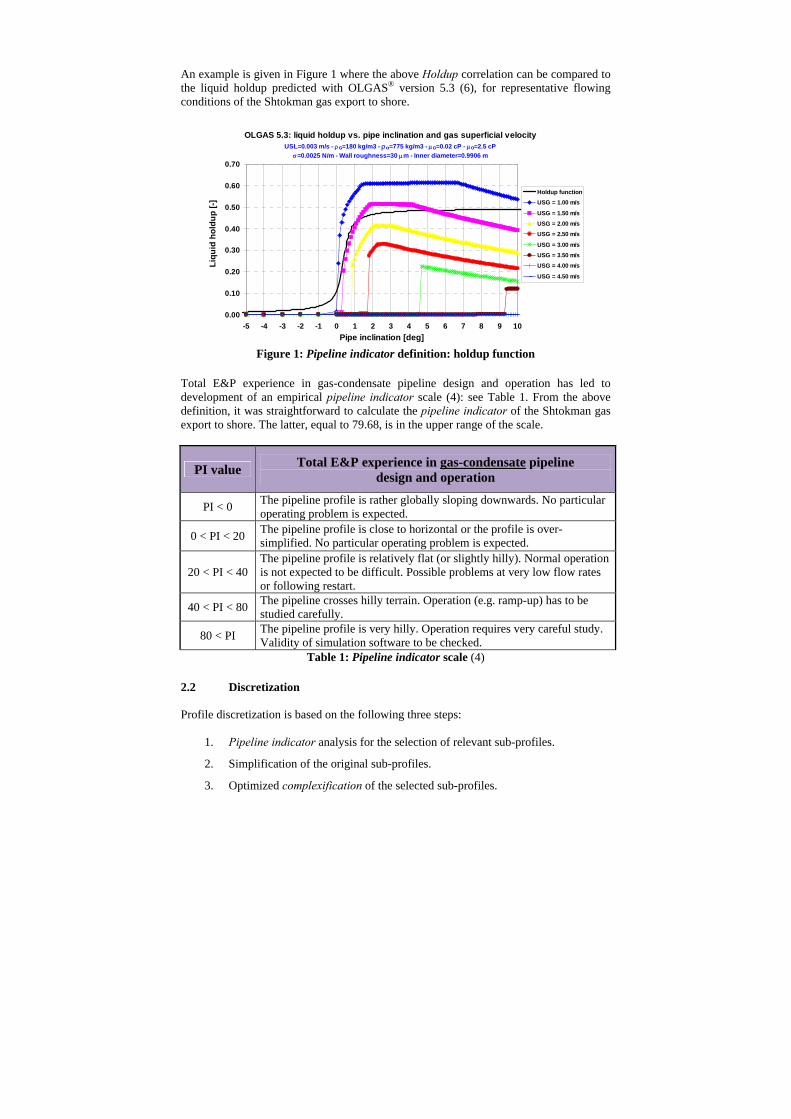
5.2 Steady-state pre-processor vs. dynamic simulation Unlike point model simulation with OLGA® steady-state pre-processor, the results from dynamic simulation are dependent on the sectioning (or meshing) of pipes into calculation cells (or sections). This subject is outside the scope of this paper. However, it is worth demonstrating the need for data compression when simulating long gas-condensate pipelines. Two different meshes were simulated with a minimum section length around 100 m to avoid severe time step limitation by CFL criterion. In the discretization from the first presented method, each pipe was divided in two calculation cells for a total 5,530 sections. In the second discretization, the following sectioning was applied for a total 5,811 sections: three cells per upward sloping pipe and 2 cells per downward sloping pipe. The calculated condensate accumulation with respect to the gas export flow rate is given in Figure 18. When running dynamic simulation, the onset of condensate accumulation is predicted at a slightly higher gas export rate (41 instead of 39 MSm3/d). However the results are still consistent with the steady-state pre-processor simulations.
Total condensate content vs. export flow rate42" ND pipeline - Fluid: 50%J0/50%J1
0
1000
2000
3000
4000
5000
6000
7000
8000
9000
10000
30 35 40 45 50 55 60 65 70
Export flow rate [MSm3/d]
Tota
l con
dens
ate
cont
ent [
m3]
First discretization method - OLGA SS pre-processorSecond discretization method - OLGA SS pre-processorFirst discretization method - OLGA dynamicSecond discretization method - OLGA dynamic
Figure 18: OLGA® Steady-state pre-processor vs. OLGA® dynamic: total
condensate content and export riser inlet pressure
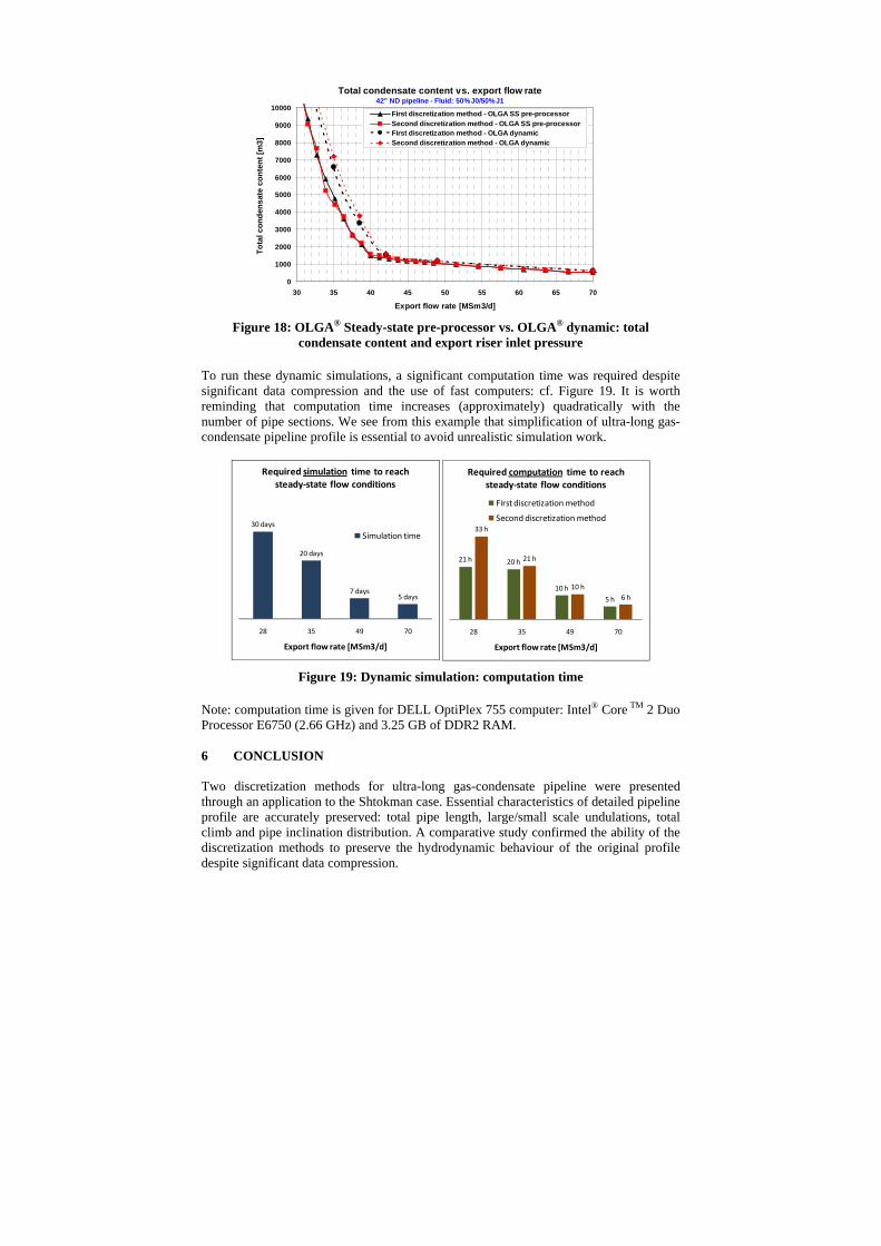
To run these dynamic simulations, a significant computation time was required despite significant data compression and the use of fast computers: cf. Figure 19. It is worth reminding that computation time increases (approximately) quadratically with the number of pipe sections. We see from this example that simplification of ultra-long gas-condensate pipeline profile is essential to avoid unrealistic simulation work.
21 h 20 h
10 h5 h
33 h
21 h
10 h6 h
28 35 49 70
Export flow rate [MSm3/d]
Required computation time to reach steady‐state flow conditions
First discretization method
Second discretization method30 days
20 days
7 days5 days
28 35 49 70
Export flow rate [MSm3/d]
Required simulation time to reach steady‐state flow conditions
Simulation time
Figure 19: Dynamic simulation: computation time
Note: computation time is given for DELL OptiPlex 755 computer: Intel® Core TM 2 Duo Processor E6750 (2.66 GHz) and 3.25 GB of DDR2 RAM. 6 CONCLUSION Two discretization methods for ultra-long gas-condensate pipeline were presented through an application to the Shtokman case. Essential characteristics of detailed pipeline profile are accurately preserved: total pipe length, large/small scale undulations, total climb and pipe inclination distribution. A comparative study confirmed the ability of the discretization methods to preserve the hydrodynamic behaviour of the original profile despite significant data compression.
This paper emphasizes the importance of gas-condensate pipeline modelling when it comes to predicting liquid accumulation for a proper design of receiving facilities. More generally, the aforementioned methods can be used either for the design of a production system, including the definition of the operating envelope, or for operation support with the simulation of actual production conditions. ACKNOWLEDGMENTS The authors would like to thank SDAG shareholders (Gazprom, Total and StatoilHydro) for their support in the preparation of this paper and their permission to publish. The authors would also like to expressly thank Doris Engineering (Geraldine Coudert and Benoit Jacob) for their valuable help with dynamic simulation. REFERENCES (1) Langsholt, M. and Holm, H., “Oil-water-gas flow in steeply inclined pipes”, BHR
Group, 10th International Conference on Multiphase Technology, Cannes, France, 2001
(2) Eidsmoen, H., Roberts, I., “Issues relating to proper modelling of the profile of long gas condensate pipelines”, PSIG paper 0501, Pipeline Simulation Interest Group, Annual Meeting, San Antonio, Texas, November 7-9, 2005
(3) OLGA®, User manual, Transient multiphase flow simulator, Version 5, 2006 (4) Barrau, B., “Profile indicator helps predict pipeline holdup, slugging”, Oil & Gas
Journal, Vol. 98, Issue 8, p. 58-62, Feb 21, 2000
(5) Kvandal, H., Munaweera, S., Elseth, G. and Holm, H., “Two-Phase Gas-Condensate Flow in Inclined Pipes at High Pressure”, Paper SPE 77505, SPE Annual Technical Conference and Exhibition held in San Antonio, Texas, 29 September–2 October 2002.
(6) OLGA® Multiphase Toolkit, version 5.3 (7) Numerical RecipesTM, 2nd edition ANSI C